Spectral gaps in a double-periodic perforated
Neumann waveguide

1  Introduction

In this section, we formulate the spectral problem under consideration, cf. Section 1.1, and provide some background which relates it with a parametric family of homogenization problems, the so-called model problem. In Section 1.3 we provide the structure of the paper while its framework in the literature is in Section 1.2.

1.1  Formulation of the problem

Let

$$\Pi=\{x=(x_{1},x_{2})\in{\mathbb{R}}^{2}:\,x_{1}\in{\mathbb{R}},x_{2}\in(0,H)\}$$ (1.1)

be an open strip of width $H>0$ and let $\omega$ be a domain in the plane ${\mathbb{R}}^{2}$ which is bounded by a smooth simple closed curve $\partial\omega$ and has the compact closure $\overline{\omega}=\omega\cup\partial\omega$ inside $\Pi$. Let $\varepsilon=N^{-1}$ where $N$ is a large natural number. We introduce the strip $\Pi^{\varepsilon}$, see Figure 1 a), obtained from $\Pi$ perforated by the family of holes

$$\omega^{\varepsilon}(j,k)=\{x:\,\varepsilon^{-1}(x_{1}-j,x_{2}-\varepsilon kH)\in\omega\},\quad j\in{\mathbb{Z}},\,\,k=0,1,\dots,N-1,$$ (1.2)

distributed periodically along line segments parallel to the ordinate $x_{2}$-axis. Each hole is homothetic to $\omega$ of ratio $\varepsilon$ and translation of $\varepsilon\omega=\omega^{\varepsilon}(0,0).$ Namely,

$$\Pi^{\varepsilon}=\Pi\setminus\overline{\Omega^{\varepsilon}}\quad\mbox{\rm where}\quad\Omega^{\varepsilon}=\bigcup\limits_{j\in{\mathbb{Z}}}\bigcup\limits_{k=0}^{N-1}\omega^{\varepsilon}(j,k).$$ (1.3)

The period of perforation along the abscissa $x_{1}$-axis in the domain $\Pi^{\varepsilon}$ is made equal to one by rescaling, which also fixes the dimensionless width $H>0$. The period along the $x_{2}$-axis is $\varepsilon H$ with $\varepsilon\ll 1.$

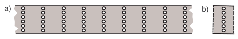
Figure 1: a) The perforated strip $\Pi^{\varepsilon}$. b) The periodicity cell $\varpi^{\varepsilon}$.

We consider the spectral Neumann problem

$$-\Delta_{x}u^{\varepsilon}(x)=\lambda^{\varepsilon}u^{\varepsilon}(x),\,\,x\in\Pi^{\varepsilon},$$ (1.4)

$$\partial_{\nu}u^{\varepsilon}(x)=0,\,\,x\in\partial\Pi^{\varepsilon},$$ (1.5)

where $\partial_{\nu}$ is the directional derivative along the outward normal while $\partial_{\nu}=\pm\partial/\partial x_{2}$ at the lateral sides $\Upsilon_{\pm}=\{x:\,x_{1}\in{\mathbb{R}},x_{2}=(H\pm H)/2\}$ of the strip (1.1). The variational formulation of the problem (1.4), (1.5) reads: to find a function $u^{\varepsilon}$ in the Sobolev space $H^{1}(\Pi^{\varepsilon})$, $u^{\varepsilon}\not\equiv 0$, and a number $\lambda^{\varepsilon}\in{\mathbb{C}}$ such that the integral identity

$$\begin{array}[]{c}(\nabla_{x}u^{\varepsilon},\nabla_{x}v^{\varepsilon})_{\Pi^{\varepsilon}}=\lambda^{\varepsilon}(u^{\varepsilon},v^{\varepsilon})_{\Pi^{\varepsilon}}\quad\forall v^{\varepsilon}\in H^{1}(\Pi^{\varepsilon})\end{array}$$ (1.6)

is valid, cf. [19]. Here, $\nabla_{x}=\mbox{\rm grad}$, $\Delta_{x}=\nabla_{x}\cdot\nabla_{x}$ is the Laplace operator and $(\,,)_{\Pi^{\varepsilon}}$ stands for the natural scalar product in the Lebesgue space $L^{2}(\Pi^{\varepsilon})$.

Since the bi-linear form on the left of (1.6) is positive, symmetric, and closed in $H^{1}(\Pi^{\varepsilon})$, problem (1.6) is associated with a positive self-adjoint operator $A^{\varepsilon}$ in the Hilbert space $L^{2}(\Pi^{\varepsilon})$ with the domain

$${\cal D}(A^{\varepsilon})=\{u^{\varepsilon}\in H^{2}(\Pi^{\varepsilon}):\,\eqref{(5)}\,\,\mbox{\rm is verified}\}.$$

Clearly, the spectrum $\sigma(A^{\varepsilon})$ belongs to the closed real positive semi-axis $[0,+\infty)=\overline{{\mathbb{R}}_{+}}\subset{\mathbb{C}}$. Moreover, according to the Floquet–Bloch–Gelfand theory, see for instance [40, 42, 33, 18, 1], the spectrum gets the band-gap structure

$$\begin{array}[]{c}\sigma(A^{\varepsilon})=\bigcup\limits_{p\in{\mathbb{N}}}\beta_{p}^{\varepsilon}\,,\end{array}$$ (1.7)

where the bands $\beta_{p}^{\varepsilon}$ are connected and compact sets in $\overline{{\mathbb{R}}_{+}}=[0,+\infty)$. The $\beta_{p}^{\varepsilon}$ are related to the eigenvalues, cf. (2.9), of the model problem in the periodicity cell

$$\begin{array}[]{c}\varpi^{\varepsilon}=\{x\in\Pi^{\varepsilon}:\,|x_{1}|<1/2\},\end{array}$$ (1.8)

see Figure 1 b), which itself constitutes a homogenization problem, cf. (2.2)–(2.5). The spectral bands $\beta_{p}^{\varepsilon}$ and $\beta_{p+1}^{\varepsilon}$ may intersect each other but can also be disjoint so that the spectral gap $\gamma_{p}^{\varepsilon}$ becomes open between them. Recall that an open spectral gap is recognized as a nontrivial open interval in ${\mathbb{R}}_{+}$ which is free of the essential spectrum but has both endpoints in it. If $\beta^{\varepsilon}_{p}\cap\beta^{\varepsilon}_{p+1}\not=\varnothing$, then we say that the gap $\gamma^{\varepsilon}_{p}$ is closed. In Figure 5 the open spectral gaps correspond with the projections of the shaded bands on the ordinate axis.

The main goal of our paper is to show that, under certain restrictions on the width $H$ and the perforation shape, the problem (1.4), (1.5) can get at least one open gap in its spectrum. Also, we aim to derive asymptotic formulas for the position and geometric characteristics of several bands and gaps in the low-frequency range of the spectrum. It should be mentioned that the traditional homogenization procedure in the problem (1.4), (1.5) does not help to detect open gaps. The crucial role is played by the boundary layer phenomenon, cf. Section 3, while the width of the gaps is expressed in terms of certain integral characteristics of the Neumann hole $\omega$ of unit size in the strip $\Pi$ with the periodicity conditions at its lateral sides, cf. (7.3), (7.7) and Remark 3.4. At the same time, we construct explicitly only the main correction term in the asymptotics of eigenvalues of the model problem in the periodicity cell and analyze different situations when this term is not sufficient to conclude whether a concrete spectral gap is actually open or not (see Section 8). Moreover, for a technical reason, cf. Section 4.5, and for simplification of asymptotic structures, we make the assumption

$$\omega=\{\xi=(\xi_{1},\xi_{2})\in{\mathbb{R}}^{2}:\,(\xi_{1},H-\xi_{2})\in\omega\}.$$ (1.9)

which means that the holes possess the mirror symmetry (see Figure 2). Also, for simplicity, we assume that the boundary of $\omega$ is of class $C^{\infty}.$

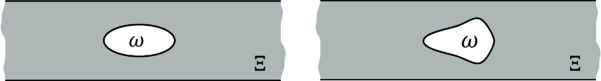
Figure 2: The strip $\Xi$ with two different possible geometries for the hole $\omega$.

1.2  State of art

The continuous spectrum in a cylindrical waveguides of different physical nature is always a ray $[\lambda_{\dagger},+\infty)$ so that, above the cutoff value $\lambda_{\dagger}\geq 0$ wave processes surely occur. The spectrum of a periodic waveguide gets far complicated band-gap structure (1.7) and the spectral bands implying passing zones for waves can be separated from each other by spectral gaps which do not permit propagation of waves with the corresponding frequencies and, therefore, become stopping zones. This phenomenon is used in different engineering devices, such as wave filters and wave dampers.

Within the Floquet–Bloch–Gelfand theory, see e.g. [8, 40, 42, 41, 18, 33, 12], mathematical studies of spectra with the band-gap structures need to find out the eigenvalues of spectral elliptic boundary value problems which are posed in the periodicity cell and involve an additional continuous parameter $\eta\in[-\pi,\pi]$, the Floquet parameter or the Gelfand dual variable. It is a very rare situation when such a problem admits explicit solutions while computational methods become rather expensive to present the whole family of dispersion curves, projections of which on the ordinate $\lambda$-axis involve the spectral bands. As usual, variational and asymptotic methods help to prove or disprove the existence of open spectral gaps in a certain range of the spectrum and to estimate their geometrical characteristics.

There are numerous publications in which open spectral gaps are detected due to high-contrast of coefficients in differential operators or shape irregularities of the periodicity cells, see [15, 16, 45, 29, 5, 4, 3, 6] and [26, 34, 39, 35, 7] among others. Such singular perturbations often provide disintegration of the periodicity cells in the limit and, as a result, the appearance of sufficiently wide gaps in the low- and/or middle-frequency ranges of the spectrum. Both variational and asymptotic methods have been employed in the cited papers to detect and describe those gaps.

Another way to open spectral gaps related to the splitting of band edges, is used in our paper. In the case when two spectral bands of the limit problem, cf. Section 2.2, intersect but just touch each other at a point, that is, there is a common edge of the bands, small perturbations of the coefficients or of the boundary may lead to a separation of these bands and the opening of a narrow gap between them, cf. Sections 6.1, 6.4, 7.1 and 7.2. This effect is well-known in the physical literature, but its mathematical study using operators theory and spectral perturbation methods started in [27, 10, 11, 31]. In this paper a new type of the singular perturbation of the periodicity cell is analyzed by means of the homogenization technique and several ways to open spectral gaps are highlighted.

Finally, let us mention that, from a geometrical viewpoint, [32] is the closest paper in the literature. It addresses the Dirichlet perforation in a quantum waveguide. The asymptotic of the spectrum of the equation (1.4), with the Dirichlet condition $u^{\varepsilon}=0$ on $\partial\Pi^{\varepsilon}$ is considered, finding out the position and sizes of the spectral gaps and bands. However, the results differ very much from those in this paper. Indeed, roughly speaking, the Dirichlet spectrum consists of small, of order $O(\varepsilon)$, spectral bands which are separated from each other by spectral gaps of width $O(1)$. In contrast, the Neumann spectrum here considered consists of long, of order $O(1)$, bands which are separated from each other by short spectral gaps of order $O(\varepsilon)$, or even less. The latter makes the asymptotic analysis much more complicated and delicate; in particular, it becomes multiscale in several variables, not only in the geometrical ones, but also in the Floquet parameter. As outlined above, the justification procedure also becomes much more complicated. For a link between the model problem in the waveguide with Neumann or Dirichlet conditions, let us mention [14].

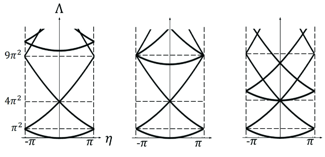
Figure 3: The dispersion curves of the limit problem in the cases $H<1/3$, $H=1/\sqrt{8}$ and $H=1/2.$

1.3  Architecture of the paper

In Section 2 we formulate the model spectral problem in the periodicity cell, b) in Figure 1, which is itself a parametric spectral homogenization problem. We obtain the homogenized problem by the classical homogenization theory in perforated media, see, e.g., [20], that is, a problem in the rectangular periodicity cell without perforations. We list explicit solutions of the homogenized problem and we study the dispersion curves which form the trusses in Figures 3 and 4, while we classify the truss nodes, namely, the crossing points of the dispersion curves. In Section 2.3, we show the convergence result for the spectrum of the model problem towards that of the homogenized one as a consequence of another stronger one, which also allows a perturbation of the Floquet-parameter.

In Section 3 we discuss the boundary layer phenomenon arising in the vicinity of the perforation. In particular, we examine several solutions of the Laplace equation in the unbounded strip $\Pi$ with the only hole $\overline{\omega}$, and we introduce the integral characteristics $m_{1}(\Xi)$, $m_{2}(\Xi)$ and $m_{3}(\Xi)$ for the Neumann problem in the domain $\Xi=\Pi\setminus{\overline{\omega}}$ (see Figure 2 and (3.1)) with the periodicity conditions on the lateral sides, cf. the traditional harmonic polarization and virtual mass tensors in the exterior domain ${\mathbb{R}}^{2}\setminus\overline{\omega}$ in [38].

In Section 4 we perform the preliminary formal asymptotic analysis for simple eigenvalues using the method of matched asymptotic expansions, cf. [43, 41, 17, 21] for two scale asymptotic expansions. In Section 5 we derive error estimates in the case of simple eigenvalues which will help us to detect open gaps after a much more thorough analysis of multiple eigenvalues. The perturbation of crossing dispersion curves require serious modifications of the standard asymptotic procedures because we can no longer deal with a fixed Floquet parameter but we must investigate the asymptotic behavior of the eigenvalues in a neighborhood of each truss node, i.e., with the Floquet parameter in a certain short interval. Recalling an idea from paper [27], in Section 6 we introduce a fast Floquet parameter to describe this behavior and detect, in different situations, open spectral gaps of width $O(\varepsilon)$, cf. Figure 5 a)–b), which appear due to splitting of the nodes marked with $\circ$ and $\square$ in Figure 4. This involves the characterization of the projections of the shaded rectangles on the ordinate axis in Figure 5, which represent the narrow gaps.

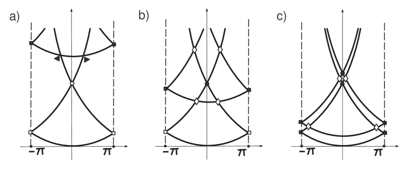
Figure 4: The dispersion curves in the limit problem in the cases a) $H\in(1/\sqrt{8},1/2)$, b) $H\in(1/2,1)$ but $H\neq 1/\sqrt{3}$ and c) $H\in(1,+\infty).$

It should be noted that our detailed calculation in Section 5 demonstrates that the first correction term in the eigenvalue asymptotics is not able to assure the gap opening and we need to discuss higher-order asymptotic terms. In fact, Section 6 is devoted to deriving the formal asymptotic analysis and its justification in the case where the eigenvalue under consideration is multiple and therefore gives rise to a node of the dispersion curves in Figure 4 a)–b) for the homogenized problem; in particular, we consider the nodes $(\eta_{\mbox{\small{$\circ$}}},\Lambda_{\mbox{\small{$\circ$}}})=(0,4\pi^{2})$ and $(\eta_{\mbox{\tiny$\square$}},\Lambda_{\mbox{\tiny$\square$}})=(\pm\pi,\pi^{2})$. Providing the error estimates for the whole range of the Floquet parameter adds the most complication to the justification scheme (see Theorems 5.1, 6.1 and 6.3). The common procedure for deriving error estimates in the homogenization theory does not support our conclusions of opening spectral gaps (see Section 7) because the model problem in the periodicity cell $\varpi^{\varepsilon}$ depends on the Floquet parameter $\eta\in[-\pi,\pi]$ and the eigenvalues (2.11) of the limit problem in $\varpi^{0}$ change their multiplicity at the nodes. As usual, to provide appropriate error estimates, we use a well-known result on almost eigenvalues and eigenfunctions from the spectral perturbation theory (see [44] and Lemma 5.3). However, we need to construct different approximations for eigenfunctions in the vicinity of the nodes and at a certain distance from them. This is performed in Sections 6.1 and 6.4. As a result, we find proper small bounds for asymptotic remainders that justify our formal computations of the band edges and gap width. It turns out that these bounds are uniform in $\eta$ but in different regions.

As regards the spectral model problem, the somehow classical convergence of the spectrum towards that of the homogenized problem is in Corollary 2.2. We obtain this result as a consequence of a more general convergence result, cf. Theorem 2.1, which allows a certain perturbation of the Floquet variable. This result is new in the literature of model problems for waveguides, and shows somehow a strong stability of the model problem on the parameter $\eta$. It becomes essential to control the number of eigenvalues below certain constants, cf. Propositions 2.3 and 2.4. Theorem 5.1 provides some estimates which establish the closeness of eigenvalues depending on $\varepsilon$ and the first three dispersion curves. As a consequence, Corollary 5.2 gives a uniform bound for the convergence rate of the first eigenvalue at a certain distance from the nodes. Theorems 6.1 and 6.3 involve a correcting term and improve convergence rates in a small neighborhood of the above mentioned nodes $(0,4\pi^{2})$ and $(\pm\pi,\pi^{2})$. Combining the results in Sections 5 and 6, in Section 7, we determine the existence of opening gaps and their width depending on $H$, cf. Theorems 7.1 and 7.2. Finally, in Section 8, we provide some hints on open problems for other nodes in Figure 4 and other geometrical configurations, cf. Figures 13 and 14.

2  The model problem in the periodicity cell

In this section, we introduce the spectral model problem and its limit problem, both of which depend on the Floquet parameter $\eta\in[-\pi,\pi]$, see Sections 2.1 and 2.2 respectively. In Section 2.3, we show the spectral convergence as $\varepsilon\to 0$, and its stability under a certain perturbation of the parameter $\eta$. In particular, this proves useful for controlling the eigenvalue number of the model problem below some bounds.

2.1  The FBG-transform and the quasi-periodicity conditions

The Floquet–Bloch–Gelfand transform (the FBG-transform in short), see [13, 40, 33, 42, 18],

$$\begin{array}[]{c}\displaystyle u^{\varepsilon}(x)\,\,\mapsto\,\,U^{\varepsilon}(x;\eta)=\frac{1}{\sqrt{2\pi}}\,\sum\limits_{p\in{\mathbb{Z}}}e^{-ip\eta}u^{\varepsilon}(x_{1}+p,x_{2})\end{array}$$ (2.1)

converts the problem (1.4), (1.5) in the infinite waveguide $\Pi^{\varepsilon}$ into a boundary value problem in the periodicity cell $\varpi^{\varepsilon}$ defined by (1.8), cf. Figure 1 b).

This problem consists of the differential equation

$$-\Delta_{x}U^{\varepsilon}(x;\eta)=\Lambda^{\varepsilon}(\eta)U^{\varepsilon}(x;\eta),\,\,x\in\varpi^{\varepsilon},$$ (2.2)

the quasi-periodicity conditions on the lateral walls

$$U^{\varepsilon}\Big{(}\frac{1}{2},x_{2};\eta\Big{)}=e^{i\eta}U^{\varepsilon}\Big{(}-\frac{1}{2},x_{2};\eta\Big{)},\,\,x_{2}\in(0,H),$$ (2.3)

$$\frac{\partial U^{\varepsilon}}{\partial x_{1}}\Big{(}\frac{1}{2},x_{2};\eta\Big{)}=e^{i\eta}\frac{\partial U^{\varepsilon}}{\partial x_{1}}\Big{(}-\frac{1}{2},x_{2};\eta\Big{)},\,\,x_{2}\in(0,H),$$ (2.4)

and the Neumann condition on the remaining part of the boundary of the periodicity cell (1.8)

$$\partial_{\nu}U^{\varepsilon}(x{\color[rgb]{0,0,0};\eta})=0,\,\,x\in\{x\in\partial\varpi^{\varepsilon}:\,|x_{1}|<1/2\}.$$ (2.5)

Here, $\eta\in[-\pi,\pi]$ is the Floquet parameter while $\Lambda^{\varepsilon}(\eta)$ and $U^{\varepsilon}(\cdot;\eta)$, respectively, are the new notations for the eigenvalues and eigenfunctions in the model problem. Notice that $x\in\Pi^{\varepsilon}$ on the left of (2.1) but $x\in\varpi^{\varepsilon}$ on the right. Basic properties of the FBG-transform can be found in the above-cited publications.

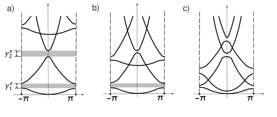
Figure 5: The dispersion curves of the perturbed problem with the mirror symmetry of the hole $\omega$ in the cases a) $H\in(1/\sqrt{8},1/2)$, b) $H\in(1/2,1)$ but $H\neq 1/\sqrt{3}$ and c) $H\in(1,+\infty).$ Spectral gaps are the projections of the shaded rectangles on the ordinate $\Lambda$-axis.

The variational statement of the problem (2.2)–(2.5) appeals to the integral identity [19]

$$\begin{array}[]{c}(\nabla_{x}U^{\varepsilon},\nabla_{x}V^{\varepsilon})_{\varpi^{\varepsilon}}=\Lambda^{\varepsilon}(U^{\varepsilon},V^{\varepsilon})_{\varpi^{\varepsilon}}\quad\forall V^{\varepsilon}\in H^{1,\eta}_{per}(\varpi^{\varepsilon}),\end{array}$$ (2.6)

where $H^{1,\eta}_{per}(\varpi^{\varepsilon})$ is the Sobolev space of functions satisfying the stable quasi-periodicity conditions (2.3) and (2.4). In view of the compact embedding $H^{1}(\varpi^{\varepsilon})\subset L^{2}(\varpi^{\varepsilon})$, the positive self-adjoint operator $A^{\varepsilon}(\eta)$ in $L^{2}(\varpi^{\varepsilon})$ associated with the problem (2.6), cf. [9, Section 10.2], has a discrete spectrum constituting the unbounded monotone sequence of eigenvalues

$$\begin{array}[]{c}0\leq\Lambda^{\varepsilon}_{1}(\eta)\leq\Lambda^{\varepsilon}_{2}(\eta)\leq\dots\leq\Lambda^{\varepsilon}_{p}(\eta)\leq\dots\to+\infty,\quad{\color[rgb]{0,0,0}\mbox{ as }p\to+\infty},\end{array}$$ (2.7)

where their multiplicity is taken into account. Furthermore, the functions

$$\begin{array}[]{c}[-\pi,\pi]\ni\eta\,\,\mapsto\,\,\Lambda^{\varepsilon}_{p}(\eta),\quad p\in{\mathbb{N}},\end{array}$$ (2.8)

are continuous and $2\pi$-periodic (see again any of the above-cited references). Hence, the sets in (1.7)

$$\begin{array}[]{c}\beta^{\varepsilon}_{p}=\{\Lambda^{\varepsilon}_{p}(\eta):\,\eta\in[-\pi,\pi]\}\subset\overline{{\mathbb{R}}_{+}}\end{array}$$ (2.9)

are closed, connected, and finite segments. Indeed, formulas (1.7) and (2.9) for the spectrum of the operator $A^{\varepsilon}(\eta)$ and the boundary-value problem (1.4), (1.5) are well-known in the framework of the Floquet–Bloch–Gelfand theory.

2.2  The limit problem and the limit dispersion curves

In Section 2.3 we will prove the relationship

$$\begin{array}[]{c}\displaystyle\Lambda^{\varepsilon}_{p}(\eta)\,\,\to\Lambda^{0}_{p}(\eta)\,\,\mbox{\rm as}\,\,\varepsilon\to+0\end{array}$$ (2.10)

between entries of the sequence (2.7) and those of the sequence

$$\begin{array}[]{c}0\leq\Lambda^{0}_{1}(\eta)\leq\Lambda^{0}_{2}(\eta)\leq\dots\leq\Lambda^{0}_{p}(\eta)\leq\dots\to+\infty,\quad{\color[rgb]{0,0,0}\mbox{ as }p\to+\infty},\end{array}$$ (2.11)

which consists of eigenvalues of the limit problem in the rectangle

$$\varpi^{0}=\{x:\,|x_{1}|<1/2,\,x_{2}\in(0,H)\}$$

obtained from the periodicity cell (1.8) by filling all voids, cf. (3.2). Above, the convention of repeated eigenvalues has been adopted, and the limit problem is also referred to as homogenized problem. It involves the differential equation

$$\begin{array}[]{c}-\Delta{\color[rgb]{0,0,0}{{}_{x}}}U^{0}(x;\eta)=\Lambda^{0}(\eta)U^{0}(x;\eta),\,\,x\in\varpi^{0},\end{array}$$ (2.12)

the Neumann conditions on the horizontal sides of the rectangle

$$\begin{array}[]{c}\displaystyle\frac{\partial U^{0}}{\partial x_{2}}(x_{1},0{\color[rgb]{0,0,0};\eta})=\frac{\partial U^{0}}{\partial x_{2}}(x_{1},H{\color[rgb]{0,0,0};\eta})=0,\,\,x_{1}\in\Big{(}-\frac{1}{2},\frac{1}{2}\Big{)},\end{array}$$ (2.13)

and the quasi-periodicity conditions on its vertical sides, cf. (2.3) and (2.4),

$$\begin{array}[]{c}\displaystyle U^{0}\Big{(}\frac{1}{2},x_{2};\eta\Big{)}=e^{i\eta}U^{0}\Big{(}-\frac{1}{2},x_{2};\eta\Big{)},\\ \\ \displaystyle\frac{\partial U^{0}}{\partial x_{1}}\Big{(}\frac{1}{2},x_{2};\eta\Big{)}=e^{i\eta}\frac{\partial U^{0}}{\partial x_{1}}\Big{(}-\frac{1}{2},x_{2};\eta\Big{)},\,\,x_{2}\in(0,H).\end{array}$$ (2.14)

This problem has the following explicit eigenvalues and eigenfunctions

$$\begin{array}[]{ll}\Lambda^{0}_{jk}(\eta)=(\eta+2\pi j)^{2}+\pi^{2}\frac{k^{2}}{H^{2}},\\ &\qquad j\in{\mathbb{Z}},\,\,k\in{\mathbb{N}}_{0}={\mathbb{N}}\cup\{0\}.\\ U^{0}_{jk}(x;\eta)=e^{i(\eta+2\pi j)x_{1}}\cos\Big{(}\pi k\frac{x_{2}}{H}\Big{)},\end{array}$$ (2.15)

It should be mentioned that renumeration of the eigenvalues in (2.15) is needed to compose the monotone sequence (2.11).

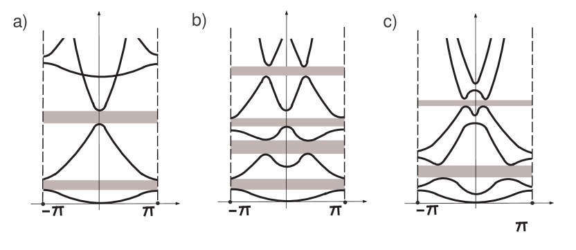
Figure 6: The hypothetical dispersion curves of the perturbed problem without the mirror symmetry of the hole $\omega$ in the cases a) $H\in(1/\sqrt{8},1/2)$, b) $H\in(1/2,1)$ but $H\neq 1/\sqrt{3}$ and c) $H\in(1,+\infty).$ Many more spectral gaps are opened than in Figure 5.

Graphs of several eigenvalues (2.15) of the problem (2.12)–(2.14), that is, the dispersion curves, are drawn in Figure 4 a)–c), respectively, for the following cases:

$$\mbox{a)}\quad H\in\Big{(}\frac{1}{\sqrt{8}},\frac{1}{2}\Big{)}\qquad\mbox{b)}\quad H\in\Big{(}\frac{1}{2},1\Big{)}\qquad\mbox{c)}\quad H\in(1,+\infty).$$

Figure 3 also displays dispersion curves of the limit problem in the cases $H\in(0,1/3)$, $H=1/\sqrt{8}$ and $H=1/2$, respectively. Figures 3 and 4 show the great variety of behaviors of the dispersion curves and, consequently, the complexity to open spectral gaps depending on $H$.

As was mentioned in Section 1.2 and depicted in Figure 5, due to the perturbation by holes of the periodicity cell, the dispersion curves for problem (2.2)–(2.5) may separate at the truss nodes marked with the signs $\square$ and $\circ$ in Figure 4 (see Section 7).

2.3  The convergence results

First, we obtain some estimates for the eigenvalues and provide an extension for eigenfunctions over the whole $\varpi^{0}$ necessary to show the convergence. The constants appearing throughout the section $c_{m}$ and $C_{m}$, are independent of both variables $\varepsilon$ and $\eta$.

Let $\eta\in[-\pi,\pi]$ be fixed and let $U^{\varepsilon}_{m}(\cdot;\eta)\in H^{1,\eta}_{per}(\varpi^{\varepsilon})$ be an eigenfunction of the problem (2.6) corresponding to the eigenvalue $\Lambda^{\varepsilon}_{m}(\eta)$. The minimax principle assures the estimate

$$\begin{array}[]{c}\displaystyle\Lambda^{\varepsilon}_{m}(\eta)\leq c_{m}\,\,\mbox{\rm for}\,\,\varepsilon\in(0,\varepsilon_{m}]\end{array}$$ (2.16)

with some positive $\varepsilon_{m}$ and $c_{m}$. Indeed, we write

$$\Lambda^{\varepsilon}_{m}(\eta)=\min_{E_{m}^{\varepsilon}\subset H^{1,\eta}_{per}(\varpi^{\varepsilon})}\max_{V\in E_{m}^{\varepsilon},V\neq 0}\frac{(\nabla_{x}V,\nabla_{x}V)_{\varpi^{\varepsilon}}}{(V,V)_{\varpi^{\varepsilon}}},$$

where the minimum is computed over the set of subspaces $E_{m}^{\varepsilon}$ of $H^{1,\eta}_{per}(\varpi^{\varepsilon})$ with dimension $m$. To prove (2.16), we take a particular $E_{m}^{\varepsilon}$ that we construct as follows: we consider the eigenfunctions corresponding to the $m$ first eigenvalues of the mixed eigenvalue problem in the rectangle $(1/4,1/2)\times(0,H)$, with Neumann condition on the part of the boundary $\{1/2\}\times(0,H)$, and Dirichlet condition on the rest of the boundary. We extend these eigenfunctions by zero for $x\in[0,1/4]\times(0,H)$, and by symmetry for $x\in[-1/2,0]\times(0,H)$. Finally, multiplying these eigenfunctions by $e^{i\eta x_{1}}$ gives $E_{m}^{\varepsilon}$ and the right hand side of (2.16) holds.

Let us construct an extension for the eigenfunctions to be uniformly bounded in $H^{1}(\varpi^{0})$. Being normalized in $L^{2}(\varpi^{\varepsilon})$, on account of (2.16), the eigenfunctions of (2.6) satisfy

$$\|\nabla_{x}U^{\varepsilon}_{m};L^{2}(\varpi^{\varepsilon})\|^{2}=\Lambda^{\varepsilon}_{m}(\eta)\|U^{\varepsilon}_{m};L^{2}(\varpi^{\varepsilon})\|^{2}=\Lambda^{\varepsilon}_{m}(\eta)\leq c_{m}\,\,\mbox{\rm for}\,\,\varepsilon\in(0,\varepsilon_{m}].$$

Therefore, we can extend $U^{\varepsilon}_{m}(\cdot;\eta)$ over the holes (3.2) and obtain a function ${\widehat{U}}^{\,\varepsilon}_{m}(\cdot;\eta)\in H^{1,\eta}_{per}(\varpi^{0})$ such that for $\varepsilon\in(0,\varepsilon_{m}]$,

$$\begin{array}[]{c}\displaystyle{\widehat{U}}^{\,\varepsilon}_{m}(x;\eta)=U^{\varepsilon}_{m}(x;\eta)\,\,\mbox{ for }x\in\varpi^{\varepsilon}\quad\mbox{ and }\vspace{0.2cm}\\ \|{\widehat{U}}^{\,\varepsilon}_{m}(\cdot;\eta);H^{1}(\varpi^{0})\|\leq C\|U^{\varepsilon}_{m};H^{1}(\varpi^{\varepsilon})\|\leq C_{m},\end{array}$$ (2.17)

see, for example, Section I.4.2 in [37] for such an extension. In addition, from (2.17) and the estimate

$$\|V;L^{2}(\varpi^{0}\cap\{|x_{1}|<\varepsilon\})\|^{2}\leq C\varepsilon\|V;H^{1}(\varpi^{0})\|^{2}\quad\forall V\in H^{1}(\varpi^{0})$$

(see, e.g., Lemma 2.4 in [22]), they satisfy

$$\begin{array}[]{c}\displaystyle\|{\widehat{U}}^{\,\varepsilon}_{m}(\cdot;\eta);L^{2}(\varpi^{0}\setminus\varpi^{\varepsilon})\|^{2}\leq c\varepsilon\|U^{\varepsilon}_{m};H^{1}(\varpi^{\varepsilon})\|^{2}\leq C_{m}\varepsilon.\end{array}$$ (2.18)

Moreover, the following results state the spectral convergence for problem (2.6), as $\varepsilon\to 0$. As a matter of fact, Theorem 2.1 also shows the stability of the limit of the spectrum of the perturbation problem (2.2)–(2.5) under any perturbation of the Floquet-parameter $\eta$.

Theorem 2.1.

For each sequence $\{(\varepsilon_{k},\eta_{k})\}_{k=1}^{\infty}$ such that $\varepsilon_{k}\to 0$ and $\eta_{k}\to\widehat{\eta}\in[-\pi,\pi]$ as $k\to+\infty$, the eigenvalues $\Lambda_{m}^{\varepsilon_{k}}(\eta_{k})$ of problem (2.2)–(2.5) when $(\varepsilon,\eta)\equiv(\varepsilon_{k},\eta_{k})$ converge, as $k\to+\infty,$ towards the eigenvalues of problem (2.12)–(2.14) for $\eta\equiv\widehat{\eta}$ and there is conservation of the multiplicity. Namely, for each $m=1,2,\cdots$, the convergence

$$\Lambda^{\varepsilon_{k}}_{m}(\eta_{k})\to\Lambda^{0}_{m}(\widehat{\eta}),\quad\mbox{ as }k\to+\infty,$$

holds, where $\Lambda^{0}_{m}(\widehat{\eta})$ is the m-th eigenvalue in the sequence

$$0\leq\Lambda^{0}_{1}(\widehat{\eta})\leq\Lambda^{0}_{2}(\widehat{\eta})\leq\dots\leq\Lambda^{0}_{m}(\widehat{\eta})\leq\dots\to+\infty,\quad\mbox{ as }m\to+\infty,$$

of eigenvalues of (2.12)–(2.14) for $\eta\equiv\widehat{\eta}$, which are counted according to their multiplicities. In addition, we can extract a subsequence, still denoted by $\varepsilon_{k}$, such that the extension $\{{\widehat{U}}_{m}^{\,\varepsilon_{k}}\}_{m=1}^{\infty}$ converge in $L^{2}(\varpi^{0})$, as $\varepsilon_{k}\to 0$, towards the eigenfunctions of (2.12)–(2.14) for $\eta\equiv\widehat{\eta}$, which form an orthonormal basis of $L^{2}(\varpi^{0})$.

Proof.

For each $\varepsilon_{k}$ and $\eta_{k}$, we write the integral equation satisfied by the eigenvalue $\Lambda_{m}^{\varepsilon_{k}}(\eta_{k})$ and corresponding eigenfunction ${U}_{m}^{\,\varepsilon_{k}}(\cdot,\eta_{k})$:

$$\begin{array}[]{c}(\nabla_{x}U_{m}^{\varepsilon_{k}},\nabla_{x}V^{\varepsilon_{k}})_{\varpi^{\varepsilon_{k}}}=\Lambda_{m}^{\varepsilon_{k}}(\eta_{k})(U_{m}^{\varepsilon_{k}},V^{\varepsilon_{k}})_{\varpi^{\varepsilon_{k}}}\quad\forall V^{\varepsilon_{k}}\in H^{1,\eta_{k}}_{per}(\varpi^{\varepsilon_{k}}),\end{array}$$ (2.19)

Since the constants appearing (2.17) and (2.18) are independent of $\eta\in[-\pi,\pi]$ and $\varepsilon$, the estimates hold $\varepsilon$ and $\eta$ ranging in sequences of $\{\varepsilon_{k}\}_{k}$ and $\{\eta_{k}\}_{k}$, in the statement of the theorem. Thus, we use an extension of $U^{\varepsilon_{k}}_{m}(\cdot;\eta)$ over the holes (3.2) denoted by ${\widehat{U}}^{\,\varepsilon_{k}}_{m}(\cdot;\eta)\in H^{1,\eta_{k}}_{per}(\varpi^{0})$, which satisfies

$$\begin{array}[]{c}\displaystyle\|{\widehat{U}}^{\,\varepsilon_{k}}_{m}(\cdot;\eta_{k});H^{1}(\varpi^{0})\|\leq C_{m},\mbox{ \quad and \quad}\vspace{0.2cm}\\ \displaystyle\|{\widehat{U}}^{\,\varepsilon_{k}}_{m}(\cdot;\eta_{k});L^{2}(\varpi^{0}\setminus\varpi^{\varepsilon_{k}})\|^{2}\leq C_{m}\varepsilon_{k}\|{U}^{\,\varepsilon_{k}}_{m}(\cdot;\eta_{k});H^{1}(\varpi^{\varepsilon_{k}})\|^{2}\leq C_{m}\varepsilon_{k};\end{array}$$ (2.20)

for sufficiently small $\varepsilon_{k}$, with a constant $C_{m}$ independent of $\varepsilon_{k}$ and $\eta_{k}$.

In view of (2.16) and (2.20), for each fixed $m\geq 1$ and for each subsequence of $k$, we can extract a subsequence, still denoted by $k$, such that

$$\begin{array}[]{c}\displaystyle\Lambda^{\varepsilon_{k}}_{m}(\eta_{k})\rightarrow\mbox{\boldmath$\widehat{\Lambda}$}^{0}_{m},\quad\mbox{as }k\to+\infty,\vspace{0.2cm}\\ \!\!{\widehat{U}}^{\,\varepsilon_{k}}_{m}(\cdot;\eta_{k})\rightarrow{\bf\widehat{U}}^{0}_{m}\,\,\mbox{\rm weakly\,\,in}\,\,H^{1}(\varpi^{0})\,\,\mbox{\rm and\,\,strongly\,\,in}\,\,L^{2}(\varpi^{0}),\quad\mbox{as }k\to+\infty,\end{array}$$ (2.21)

for some real number $\mathbf{\widehat{\Lambda}}^{0}_{m}\geq 0$ and some function ${\bf\widehat{U}}^{0}_{m}\in H^{1}(\varpi^{0})$ which we determine below depending on $\widehat{\eta}$.

We take a test function $V\in C^{\infty}(\overline{\varpi^{0}})$ verifying the periodicity condition at the lateral sides of $\varpi^{0}$ and consider $V^{k}=Ve^{i\eta_{k}x_{1}}$ which satisfies the quasi-periodicity condition in (2.14) with $\eta\equiv\eta_{k}$. For $V^{\varepsilon_{k}}\equiv V^{k}$, we rewrite the integral identity (2.19) in the form

$$(\nabla_{x}{\widehat{U}}^{\,\varepsilon_{k}}_{m},\nabla_{x}V^{k})_{\varpi^{0}}-\Lambda^{\varepsilon_{k}}_{m}(\eta_{k})({\widehat{U}}^{\,\varepsilon_{k}}_{m},V^{k})_{\varpi^{0}}=(\nabla_{x}{\widehat{U}}^{\,\varepsilon_{k}}_{m},\nabla_{x}V^{k})_{\varpi^{0}\setminus\varpi^{\varepsilon_{k}}}-\Lambda^{\varepsilon_{k}}_{m}(\eta)({\widehat{U}}^{\,\varepsilon_{k}}_{m},V^{k})_{\varpi^{0}\setminus\varpi^{\varepsilon_{k}}}.$$ (2.22)

According to (2.20) and (2.16), the modulo of the right-hand side of (2.22) does not exceed

$$\begin{array}[]{c}\displaystyle(1+c_{m}\varepsilon_{k})\|{\widehat{U}}^{\,\varepsilon_{k}}_{m};H^{1}(\varpi^{0})\|\,\|V^{k};H^{1}(\varpi^{0}\setminus\varpi^{\varepsilon_{k}})\|\leq c_{m}(V^{k})\mbox{\rm mes}_{2}(\varpi^{0}\setminus\varpi^{\varepsilon_{k}})\\ \\ \leq c_{m}\max_{x\in\overline{\varpi^{0}}}(|V^{k}(x)|,|\partial_{x_{1}}V^{k}(x)|,|\partial_{x_{2}}V^{k}(x)|)\varepsilon_{k}\leq C_{m}(V)(1+\eta_{k})\varepsilon_{k}.\end{array}$$ (2.23)

Thus, the right hand side of (2.22) converges towards zero as $k\to+\infty$. Let us analyze the left hand side in further detail.

In order to do this, let us consider the well-known change $\widehat{U}_{m}^{\varepsilon_{k}}(\cdot;\eta_{k})=V_{m}^{\varepsilon_{k}}(\cdot;\eta_{k})e^{i\eta_{k}x_{1}}$ which converts the Laplacian into the differential operator

$$-\Big{(}\frac{\partial}{\partial x_{1}}+i\eta\Big{)}\Big{(}\frac{\partial}{\partial x_{1}}+i\eta\Big{)}-\frac{\partial^{2}}{\partial x_{2}^{2}},$$

while the $\eta_{k}$ quasi-periodicity condition for $\widehat{U}_{m}^{\varepsilon_{k}}(\cdot;\eta_{k})$ becomes a periodicity condition for $V_{m}^{\varepsilon_{k}}(\cdot;\eta_{k})$. Consequently, $V_{m}^{\varepsilon_{k}}(\cdot;\eta_{k})\in H^{1}_{per}(\varpi^{0})$ and since $\eta_{k}\to\widehat{\eta}$ as $k\to+\infty$ (equivalently, $\varepsilon_{k}\to 0$), we also have the bound for $V_{m}^{\varepsilon_{k}}$ in $H^{1}_{per}(\varpi^{0})$ which holds uniformly in $\eta_{k}$ and $\varepsilon_{k}$, and a convergence of $V_{m}^{\varepsilon_{k}}$ (by subsequences, still denoted by $k$) towards a function $V^{0}_{m}\in H^{1}_{per}(\varpi^{0})$ holds in the weak topology of $H^{1}(\varpi^{0})$. Let us show that

$$V_{m}^{0}={\bf\widehat{U}}_{m}^{0}e^{-i\widehat{\eta}x_{1}}.$$ (2.24)

To do this, it suffices to show

$$\|\widehat{U}_{m}^{\varepsilon_{k}}(\cdot;\eta_{k})e^{-i\eta_{k}x_{1}}-{\bf\widehat{U}}_{m}^{0}e^{-i\widehat{\eta}x_{1}};L^{2}(\varpi^{0})\|\to 0\quad\mbox{ as }k\to+\infty,$$

and we check this by considering

$$\begin{split}&\|\widehat{U}_{m}^{\varepsilon_{k}}(\cdot;\eta_{k})e^{-i\eta_{k}x_{1}}-{\bf\widehat{U}}_{m}^{0}e^{-i\widehat{\eta}x_{1}};L^{2}(\varpi^{0})\|\\ &\quad\leq\|\big{(}\widehat{U}_{m}^{\varepsilon_{k}}(\cdot;\eta_{k})-{\bf\widehat{U}}_{m}^{0}\big{)}e^{-i\eta_{k}x_{1}};L^{2}(\varpi^{0})\|+\|{\bf\widehat{U}}_{m}^{0}\big{(}e^{-i\eta_{k}x_{1}}-e^{-i\widehat{\eta}x_{1}}\big{)};L^{2}(\varpi^{0})\|,\end{split}$$

the convergence (2.21), the smoothness of the exponential function and the convergence of $\eta_{k}$.

Introducing the change $V^{k}=Ve^{i\eta_{k}x_{1}}$ in (2.22), we write

$$\begin{array}[]{l}\displaystyle(\nabla_{x}{\widehat{U}}^{\,\varepsilon_{k}}_{m},\nabla_{x}(Ve^{i\eta_{k}x_{1}}))_{\varpi^{0}}-\Lambda^{\varepsilon_{k}}_{m}(\eta_{k})({\widehat{U}}^{\,\varepsilon_{k}}_{m},Ve^{i\eta_{k}x_{1}})_{\varpi^{0}}\vspace{0.2cm}\\ =(\nabla_{x}{\widehat{U}}^{\,\varepsilon_{k}}_{m},\nabla_{x}(Ve^{i\widehat{\eta}x_{1}}))_{\varpi^{0}}+(\nabla_{x}{\widehat{U}}^{\,\varepsilon_{k}}_{m},\nabla_{x}(V(e^{i\eta_{k}x_{1}}-e^{i\widehat{\eta}x_{1}})))_{\varpi^{0}}\vspace{0.2cm}\\ \quad-\Lambda^{\varepsilon_{k}}_{m}(\eta_{k})({\widehat{U}}^{\,\varepsilon_{k}}_{m},Ve^{i\widehat{\eta}x_{1}})_{\varpi^{0}}-\Lambda^{\varepsilon_{k}}_{m}(\eta_{k})({\widehat{U}}^{\,\varepsilon_{k}}_{m},V(e^{i\eta_{k}x_{1}}-e^{i\widehat{\eta}x_{1}}))_{\varpi^{0}}\,.\end{array}$$ (2.25)

Let us show

$$Ve^{i\eta_{k}x_{1}}\to Ve^{i\widehat{\eta}x_{1}}\mbox{ in }H^{1}(\varpi^{0})\quad\mbox{ as }k\to+\infty$$ (2.26)

and therefore, from (2.21), also the convergence

$$(\nabla_{x}{\widehat{U}}^{\,\varepsilon_{k}}_{m},\nabla_{x}(V(e^{i\eta_{k}x_{1}}-e^{i\widehat{\eta}x_{1}})))_{\varpi^{0}}-\Lambda^{\varepsilon_{k}}_{m}(\eta_{k})({\widehat{U}}^{\,\varepsilon_{k}}_{m},V(e^{i\eta_{k}x_{1}}-e^{i\widehat{\eta}x_{1}})))_{\varpi^{0}}\mathop{\displaystyle{\stackrel{{\scriptstyle\scriptstyle{k\to+\infty}}}{{\hbox to40.0pt{\rightarrowfill}}}}}0,$$

holds. Indeed, on account of the smoothness of $V$, we have

$$\begin{split}&\|V(e^{i\eta_{k}x_{1}}-e^{i\widehat{\eta}x_{1}});H^{1}(\varpi^{0})\|^{2}\\ &\,\,\leq C(V)\Big{(}\|e^{i\eta_{k}x_{1}}-e^{i\widehat{\eta}x_{1}};L^{2}(\varpi^{0})\|^{2}+\|\eta_{k}e^{i\eta_{k}x_{1}}-\widehat{\eta}e^{i\widehat{\eta}x_{1}};L^{2}(\varpi^{0})\|^{2}\Big{)}\mathop{\displaystyle{\stackrel{{\scriptstyle\scriptstyle{k\to+\infty}}}{{\hbox to40.0pt{\rightarrowfill}}}}}0,\end{split}$$

for a certain positive constant $C(V)$, and this shows (2.26).

Then, taking limits in (2.25) as $k\to\infty$, on account of (2.21), (2.23), (2.26) and (2.24), we obtain the integral identity

$$(\nabla_{x}{\bf\widehat{U}}^{0}_{m},\nabla_{x}(Ve^{i\widehat{\eta}x_{1}}))_{\varpi^{0}}-\mbox{\boldmath$\widehat{\Lambda}$}^{0}_{m}({\bf\widehat{U}}^{0}_{m},Ve^{i\widehat{\eta}x_{1}})_{\varpi^{0}}=0\quad\forall V\in C^{\infty}(\overline{\varpi^{0}})\cap H^{1}_{per}(\varpi^{0}),$$

while, by a completion argument, we can write

$$(\nabla_{x}{\bf\widehat{U}}^{0}_{m},\nabla_{x}(Ve^{i\widehat{\eta}x_{1}}))_{\varpi^{0}}-\mbox{\boldmath$\widehat{\Lambda}$}^{0}_{m}({\bf\widehat{U}}^{0}_{m},Ve^{i\widehat{\eta}x_{1}})_{\varpi^{0}}=0\quad\forall V\in H^{1}_{per}(\varpi^{0}),$$

or equivalently,

$$(\nabla_{x}{\bf\widehat{U}}^{0}_{m},\nabla_{x}V)_{\varpi^{0}}-\mbox{\boldmath$\widehat{\Lambda}$}^{0}_{m}({\bf\widehat{U}}^{0}_{m},V)_{\varpi^{0}}=0\quad\forall V\in H^{1,\widehat{\eta}}_{per}(\varpi^{0}).$$ (2.27)

On account of (2.24), also ${\bf\widehat{U}}_{m}^{0}\in H^{1,\widehat{\eta}}_{per}(\varpi^{0})$ and, consequently, (2.27) is nothing but the weak formulation of (2.12)–(2.14) for $\eta\equiv\widehat{\eta}$.

Furthermore,

$$1=\|U^{\varepsilon_{k}}_{m}(\cdot,\eta_{k});L^{2}(\varpi^{\varepsilon_{k}})\|^{2}=\|{\widehat{U}}^{\,\varepsilon_{k}}_{m}(\cdot,\eta_{k});L^{2}(\varpi^{0})\|^{2}-\|{\widehat{U}}^{\,\varepsilon_{k}}_{m}(\cdot,\eta_{k});L^{2}(\varpi^{0}\setminus\varpi^{\varepsilon_{k}})\|^{2}$$

and taking limits as $k\to+\infty$, on account of (2.20) and (2.21), gives

$$\|{\bf\widehat{U}}^{0}_{m};L^{2}(\varpi^{0})\|^{2}=1.$$

This, together with (2.27), identifies $(\mbox{\boldmath$\widehat{\Lambda}$}^{0}_{m},{\bf\widehat{U}}_{m}^{0})$ with an eigenpair of (2.12)–(2.14) when $\eta\equiv\widehat{\eta}$.

Therefore, we conclude that ${\bf\widehat{\Lambda}}_{m}^{0}$ is an eigenvalue with the corresponding eigenfunction ${\bf\widehat{U}}_{m}^{0}$ of the limit problem (2.12)–(2.14) when $\eta\equiv\widehat{\eta}$, and we get a dependence of ${\bf\widehat{\Lambda}}^{0}_{m}$ on $\widehat{\eta}$, so we write ${\bf\widehat{\Lambda}}^{0}_{m}:={\bf\widehat{\Lambda}}^{0}_{m}(\widehat{\eta})$.

Note that the extracted subsequences and limits may depend on $m$. However, using a diagonalization argument, for each sequence of $k$, we can extract another subsequence, still denoted by $k$, but independent of $m$, such that (2.21) holds $\forall m\in{\mathbb{N}}$. Then, by the construction, we have obtained an increasing sequence

$$0\leq{\bf\widehat{\Lambda}}^{0}_{1}(\widehat{\eta})\leq{\bf\widehat{\Lambda}}^{0}_{2}(\widehat{\eta})\leq\dots\leq{\bf\widehat{\Lambda}}^{0}_{m}(\widehat{\eta})\leq\dots.$$ (2.28)

In what follows we prove that the sequence $\{{\bf\widehat{\Lambda}}^{0}_{m}(\widehat{\eta})\}_{m=1}^{\infty}$ converges towards infinity while the whole sequence coincides with that in (2.11) when $\eta\equiv\widehat{\eta}$.

From the orthogonality of $U^{\varepsilon_{k}}_{m}(\cdot;\eta_{k})$ in $L^{2}(\varpi^{\varepsilon_{k}})$, we write

$$({\widehat{U}}^{\,\varepsilon_{k}}_{m}(\cdot;\eta_{k}),{\widehat{U}}^{\,\varepsilon_{k}}_{n}(\cdot;\eta_{k}))_{\varpi^{0}}=({\widehat{U}}^{\,\varepsilon_{k}}_{m}(\cdot;\eta_{k}),{\widehat{U}}^{\,\varepsilon_{k}}_{n}(\cdot;\eta_{k}))_{\varpi^{0}\setminus\varpi^{\varepsilon_{k}}}\quad\forall m,n\in{\mathbb{N}},\,\,m\not=n$$

and use (2.20) to get the orthogonality of the eigenfunctions $\{{\bf\widehat{U}}^{0}_{m}\}_{m=1}^{\infty}$ in $L^{2}(\varpi^{0})$. This shows that the sequence in (2.28) converges towards infinity as $m\to\infty$.

In order to show that with the above limits (2.28) we reach all the eigenvalues in the entry (2.11) when $\eta\equiv\widehat{\eta}$, namely, that $\Lambda^{0}_{m}(\widehat{\eta})=\mathbf{\widehat{\Lambda}}^{0}_{m}(\widehat{\eta})$, it suffices to show that the set $\{{\bf\widehat{U}}^{0}_{m}\}_{m=1}^{\infty}$ forms a basis of $L^{2}(\varpi^{0})$. Indeed, this is a classical process of contradiction (see, for instance, Section III.1 of [37] and Section III.9.1 of [2]). In this way, we have proved that (2.10) holds for any $p\in\mathbb{N}$, where $\{{\bf\widehat{\Lambda}}^{0}_{p}(\widehat{\eta})\}_{p=1}^{\infty}$ are the set of eigenvalues of (2.12)–(2.14) when $\eta\equiv\widehat{\eta}$ and the eigenfunctions $\{{\bf\widehat{U}}^{0}_{p}\}_{p=1}^{\infty}$ form an orthonormal basis of $L^{2}(\varpi^{0})$. Consequently, the sequence (2.28) coincides with (2.11), and the theorem is proved. ∎

Corollary 2.2.

For any $\eta\in[-\pi,\pi]$, the eigenvalues $\Lambda_{m}^{\varepsilon}(\eta)$ of problem (2.2)–(2.5) in the sequence (2.7) converge, as $\varepsilon\to+0,$ towards the eigenvalues of problem (2.12)–(2.14) in the sequence (2.11) and there is conservation of the multiplicity. In addition, for each sequence, we can extract a subsequence, still denoted by $\varepsilon$, such that the extensions $\{{\widehat{U}}_{m}^{\,\varepsilon}\}_{m=1}^{\infty}$ converge in $L^{2}(\varpi^{0})$, as $\varepsilon\to 0$, towards the eigenfunctions of (2.12)–(2.14), which form an orthonormal basis of $L^{2}(\varpi^{0})$. Also, for each eigenfunction $U_{p}^{0}$ of (2.12)–(2.14) associated with the eigenvalue $\Lambda_{p}^{0}(\eta)$ of multiplicity $n_{p}$, $\Lambda_{p}^{0}(\eta)=\Lambda_{p+1}^{0}(\eta)=\cdots=\Lambda_{p+n_{p}-1}^{0}(\eta)$ in (2.11), there is a linear combination $U^{\varepsilon}$ of eigenfunctions corresponding to the eigenvalues $\Lambda_{p}^{\varepsilon}(\eta),\,\Lambda_{p+1}^{\varepsilon}(\eta),\,\dots,\,\Lambda_{p+n_{p}-1}^{\varepsilon}(\eta)$ in (2.7), that converges towards $U_{p}^{0}$ in $L^{2}(\omega).$

Proof.

The first two assertions hold from Theorem 2.1 taking $\eta_{k}\equiv\eta$ fixed for all $k$ with minor modifications. Moreover, the last result is obtained using the technique in Theorem III.1.7 in [37]. ∎

In addition to the bounds (2.16), we state the following lower bounds for the first eigenvalues of problem (2.6).

Proposition 2.3.

Let $H\in(0,1)$. Let $\delta_{1}>0$ (and $<\pi$). Then, there exists a positive constant $\varepsilon_{1}=\varepsilon_{1}(H,\delta_{1})$ such that the entries $\Lambda^{\varepsilon}_{2}(\eta)$ and $\Lambda^{\varepsilon}_{3}(\eta)$ of the eigenvalue sequence (2.7) meet the estimates

$$\Lambda_{2}^{\varepsilon}(\eta)>\pi^{2}+K_{1}\qquad \mbox{for }\eta\in I_{1}=[-\pi+\delta_{1},\pi-\delta_{1}],\,\varepsilon<\varepsilon_{1},$$ (2.29)

$$\Lambda_{3}^{\varepsilon}(\eta)>\pi^{2}+K_{2}\qquad \mbox{for }\eta\in[-\pi,\pi],\,\varepsilon<\varepsilon_{1},$$ (2.30)

where

$$K_{1}=\min\left\{2\pi\delta_{1},\frac{\pi^{2}(1-H^{2})}{2H^{2}}\right\},\qquad K_{2}=\min\left\{2\pi^{2},\frac{2\pi^{2}(1-H^{2})}{3H^{2}}\right\}.$$ (2.31)

Proof.

We proceed by contradiction, denying (2.29). This implies that for any $\varepsilon_{1}>0$ there exist $\varepsilon<\varepsilon_{1}$ and $\eta\in I_{1}$ such that $\Lambda_{2}^{\varepsilon}(\eta)\leq\pi^{2}+K_{1}.$ It is clear that we can take a sequence $\{\varepsilon_{k}\}_{k=1}^{\infty}$ such that $\varepsilon_{k}\to 0$ as $k\to+\infty$, and an associated sequence $\{{\eta_{k}}\}_{k=1}^{\infty}$ which is bounded from above and from below, and satisfies

$$\Lambda_{2}^{\varepsilon_{k}}(\eta_{k})\leq\pi^{2}+K_{1}.$$ (2.32)

By subsequences, we can construct a sequence (still denoted by $k$) such that

$$(\eta_{k},\varepsilon_{k})\to(\widehat{\eta},0)\hbox{ as }k\to+\infty,$$

for certain $\widehat{\eta}\in I_{1}$. Let us show that this last assertion leads us to a contradiction.

According to Theorem 2.1, taking limits in (2.32), we get $\Lambda^{0}_{2}(\widehat{\eta})\leq\pi^{2}+K_{1}.$ Since $\Lambda^{0}_{2}(\widehat{\eta})$ can only be $(2\pi-|\widehat{\eta}|)^{2}$ or $(\pi/H)^{2}+|\widehat{\eta}|^{2}$ with $\widehat{\eta}\in I_{1}$, we obtain

$$\min\left\{(\pi+\delta_{1})^{2},\frac{\pi^{2}}{H^{2}}\right\}\leq\Lambda^{0}_{2}(\widehat{\eta})\leq\pi^{2}+K_{1},$$

and this contradicts the hypothesis on the chosen $K_{1}$. Consequently, (2.29) is proved.

Analogously, we proceed by contradiction, denying (2.30). Thus, as in the proof of (2.29), there exists $\widehat{\eta}\in[-\pi,\pi]$ such that $\Lambda^{0}_{3}(\widehat{\eta})\leq\pi^{2}+K_{2}.$ Since $\Lambda^{0}_{3}(\widehat{\eta})$ can be only $(2\pi+|\widehat{\eta}|)^{2}$ or $(\pi/H)^{2}+|\widehat{\eta}|^{2}$ ($\widehat{\eta}\in[-\pi,\pi]),$

$$\min\left\{4\pi^{2},\frac{\pi^{2}}{H^{2}}\right\}\leq\Lambda^{0}_{3}(\widehat{\eta})\leq\pi^{2}+K_{2},$$

and this contradicts the hypothesis on the chosen $K_{2}$. ∎

Proposition 2.4.

Let $H\in(0,1/2)$. Let $\delta_{3}>0$ (and $<\pi$). Then, there exists a positive constant $\varepsilon_{1}=\varepsilon_{1}(H,\delta_{3})$ such that the entries $\Lambda^{\varepsilon}_{3}(\eta)$ and $\Lambda^{\varepsilon}_{4}(\eta)$ of the eigenvalue sequence (2.7) meet the estimates

$$\Lambda_{3}^{\varepsilon}(\eta)>4\pi^{2}+K_{3}\qquad \mbox{for }\eta\in I_{3}=[-\pi,-\delta_{3}]\cup[\delta_{3},\pi],\,\varepsilon<\varepsilon_{1},$$ (2.33)

$$\Lambda_{4}^{\varepsilon}(\eta)>4\pi^{2}+K_{4}\qquad \mbox{for }\eta\in[-\pi,\pi],\,\varepsilon<\varepsilon_{1},$$ (2.34)

where

$$K_{3}=\min\left\{4\pi\delta_{3},\frac{\pi^{2}(1-4H^{2})}{H^{2}}\right\}>0,\qquad K_{4}=\min\left\{4\pi^{2},\frac{\pi^{2}(1-4H^{2})}{2H^{2}}\right\}>0.$$ (2.35)

Proof.

First we prove (2.33) with the same analysis as in Proposition 2.3. We proceed by contradiction, denying (2.33). Thus, as in the proof of (2.29), there exists $\widehat{\eta}\in I_{3}$ such that $\Lambda^{0}_{3}(\widehat{\eta})\leq 4\pi^{2}+K_{3}.$ Since $H<1/2$, $\Lambda^{0}_{3}(\widehat{\eta})$ can only be $(2\pi+|\widehat{\eta}|)^{2}$ or $(\pi/H)^{2}+|\widehat{\eta}|^{2}$ ($\widehat{\eta}\in I_{3}$). Therefore, we get

$$\min\left\{(2\pi+\delta_{3})^{2},\frac{\pi^{2}}{H^{2}}+\delta^{2}_{3}\right\}\leq\Lambda^{0}_{3}(\widehat{\eta})\leq 4\pi^{2}+K_{3},$$

and this contradicts the hypothesis on the chosen $K_{3}$.

Finally, we proceed by contradiction, denying (2.34). Thus, as in the proof of (2.29), there exists $\widehat{\eta}\in[-\pi,\pi]$ such that $\Lambda^{0}_{4}(\widehat{\eta})\leq 4\pi^{2}+K_{4}.$ Since $H<1/2$, $\Lambda^{0}_{4}(\widehat{\eta})$ can only be $(4\pi-|\widehat{\eta}|)^{2}$ or $(\pi/H)^{2}+|\widehat{\eta}|^{2}$ for $\widehat{\eta}\in[-\pi,\pi]$. Therefore, we get

$$\min\left\{9\pi^{2},\frac{\pi^{2}}{H^{2}}\right\}\leq\Lambda^{0}_{4}(\widehat{\eta})\leq 4\pi^{2}+K_{4},$$

and this contradicts the hypothesis on the chosen $K_{4}$. ∎

3  The boundary layer phenomenon in the periodicity cell

The traditional results of the homogenization theory given in Corollary 2.2 do not help to conclude on the splitting of band edges and in this section we examine special solutions of a boundary-value problem in the strip $\Pi$ with the only hole $\overline{\omega}$ of unit size. Let us define

$$\Xi:=\Pi\setminus\overline{\omega}\,.$$ (3.1)

Although we apply these solutions under the symmetry assumption (1.9), we only use it in Section 3.4; see Figure 2.

3.1  The problems in $\Xi$ and their solvability

According to [32], near the perforation string

$$\begin{array}[]{c}\displaystyle\omega^{\varepsilon}(0,0),\dots,\omega^{\varepsilon}(0,N-1)\subset\varpi^{0}=\{x:\,{\color[rgb]{0,0,0}|x_{1}|<1/2},x_{2}\in(0,H)\},\end{array}$$ (3.2)

cf., (1.2), there appears a boundary layer which is described in the stretched coordinates

$$\begin{array}[]{c}\xi=(\xi_{1},\xi_{2})=\varepsilon^{-1}{\color[rgb]{0,0,0}(x_{1},x_{2}-\varepsilon kH)}\end{array}$$ (3.3)

by means of a family of special solutions to the Laplace equation

$$\begin{array}[]{c}-\Delta_{\xi}W(\xi)=0,\,\,\xi\in{\color[rgb]{0,0,0}\Xi,}\end{array}$$ (3.4)

or the Poisson equation

$$\begin{array}[]{c}\displaystyle-\Delta_{\xi}W(\xi)=F(\xi),\,\,\xi\in{\color[rgb]{0,0,0}\Xi},\end{array}$$ (3.5)

with the periodicity conditions

$$\begin{array}[]{c}\displaystyle W(\xi_{1},H)=W(\xi_{1},0),\,\,\frac{\partial W}{\partial\xi_{2}}(\xi_{1},H)=\frac{\partial W}{\partial\xi_{2}}(\xi_{1},0),\,\,\xi_{1}\in{\mathbb{R}},\end{array}$$ (3.6)

and the Neumann condition on the boundary of the hole $\overline{\omega}$ inside the strip (1.1), either homogeneous

$$\begin{array}[]{c}\partial_{\nu(\xi)}W(\xi)=0,\,\,\xi\in\partial\omega,\end{array}$$ (3.7)

or inhomogeneous

$$\begin{array}[]{c}\displaystyle\partial_{\nu(\xi)}W(\xi)=G(\xi),\,\,\xi\in\partial\omega,\end{array}$$ (3.8)

with particular functions $F(\xi)$ and $G(\xi)$. Here, $\nu(\xi)=(\nu_{1}(\xi),\nu_{2}(\xi))$ is the outward (with respect to $\Xi$) normal vector on $\partial\omega$ and, therefore, the inward one with respect to $\omega$.

Remark 3.1.

The boundary condition (3.7) is directly inherited from the original condition (1.5) on the boundary of the perforation string (3.2). For any $\Lambda^{\varepsilon}\leq C$, we have

$$\Delta_{x}+\Lambda^{\varepsilon}=\varepsilon^{-2}(\Delta_{\xi}+\varepsilon^{2}\Lambda^{\varepsilon})\,\,\mbox{\rm with}\,\,\varepsilon^{2}\Lambda^{\varepsilon}\leq C\varepsilon^{2}$$

and the main asymptotic part $\Delta_{\xi}$ of the above differential operator is involved with the Laplace equation (3.4). The periodicity conditions (3.6) have no relation to the original quasi-periodicity conditions (2.3), (2.4) but are needed to support the standard asymptotic ansatz

$$U^{\varepsilon}\approx w(x_{2})W(\varepsilon^{-1}x),$$

where $w$ is a smooth function in $x_{2}\in[0,H]$ and $W$ is a function $H$-periodic in $\xi_{2}=\varepsilon^{-1}x_{2}$.

We proceed with the variational formulation

$$\begin{array}[]{c}\displaystyle(\nabla_{\xi}W,\nabla_{\xi}V)_{\Xi}=(F,V)_{\Xi}+(G,V)_{\partial\color[rgb]{0,0,0}\omega}\quad\forall V\in{\cal H}^{1}_{per}(\Xi)\end{array}$$ (3.9)

of the Poisson equation (3.5) with the periodicity (3.6) and boundary (3.8) conditions. Here, ${\cal H}^{1}_{per}(\Xi)$ is the completion of the linear space $C^{\infty}_{per}(\overline{\Xi})$ (infinitely differentiable $H$-periodic in $\xi_{2}$ functions with compact supports) in the norm

$$\begin{array}[]{c}\displaystyle\|W;{\cal H}^{1}_{per}(\Xi)\|=\Big{(}\|\nabla_{\xi}W;L^{2}(\Xi)\|^{2}+\|W;L^{2}(\Xi(2R))\|^{2}\Big{)}^{1/2},\end{array}$$ (3.10)

where $R$ is a fixed positive constant such that

$$\begin{array}[]{c}\displaystyle\overline{\omega}\subset\Xi(R):=\{\xi\in\Xi:\,|\xi_{1}|<R\}.\end{array}$$ (3.11)

Also, for convenience, we introduce here the cut-off functions, $\chi_{\pm}\in C^{\infty}({\mathbb{R}})$,

$$\begin{array}[]{c}\displaystyle\chi_{\pm}(t)=1\,\,\mbox{\rm for}\,\,\pm t>2R\,\,\mbox{\rm and}\,\,\chi_{\pm}(t)=0\,\,\mbox{\rm for}\,\,\pm t<R,\end{array}$$ (3.12)

with a fixed $R>0$ satisfying (3.11).

Proposition 3.2.

Let the functions on the right-hand sides of the problem (3.5), (3.6), (3.8) meet the inclusions

$$\begin{array}[]{c}\displaystyle(1+\xi^{2}_{1})^{1/2}F\in L^{2}(\Xi),\quad G\in L^{2}(\partial\omega)\end{array}$$ (3.13)

and the orthogonality condition

$$\begin{array}[]{c}\displaystyle\int\limits_{\Xi}F(\xi)d\xi+\int\limits_{\partial\omega}G(\xi){\color[rgb]{0,0,0}ds_{\xi}}=0.\end{array}$$ (3.14)

Then the problem has a solution $W\in{\cal H}_{per}^{1}(\Xi)$ which is defined up to an additive constant.

Proof.

We consider the perturbed equation

$$\begin{array}[]{c}\displaystyle-\Delta_{\xi}W(\xi)+\mu X_{R}(\xi)W(\xi)=F(\xi),\,\,\xi\in{\color[rgb]{0,0,0}\Xi,}\end{array}$$ (3.15)

with the boundary conditions (3.6) and (3.8); here, $\mu>0$ is a parameter and $X_{R}$ is the characteristic function of the truncated domain $\Xi(2R)$, i.e. $X_{R}(\xi)=1$ for $|\xi_{1}|<2R$ and $X_{R}(\xi)=0$ for $|\xi_{1}|>2R$. The variational formulation of the problem (3.15), (3.8), (3.6) reads:

$$\begin{array}[]{c}\displaystyle(\nabla_{\xi}W,\nabla_{\xi}V)_{\Xi}+\mu(W,V)_{\Xi(2R)}=(F,V)_{\Xi}+(G,V)_{\partial{\color[rgb]{0,0,0}\omega}}\quad\forall V\in{\cal H}^{1}_{per}(\Xi).\end{array}$$ (3.16)

In view of the one-dimensional Hardy inequality

$$\int\limits_{R}^{+\infty}\Big{|}\frac{dZ}{d\xi_{1}}(\xi_{1})\Big{|}^{2}d\xi_{1}\geq\frac{1}{4}\int\limits_{R}^{+\infty}|Z(\xi_{1})|^{2}\,\frac{d\xi_{1}}{\xi_{1}^{2}}\quad\forall Z\in C^{\infty}_{c}(R,+\infty),$$

applied to the functions $Z(\pm\xi_{1},\xi_{2})=\chi_{\pm}(\xi_{1})W(\xi_{1},\xi_{2})$ with $\chi_{\pm}$ defined by (3.12), and integrated in $\xi_{2}\in(0,H)$, the norm (3.10) is equivalent to the norm

$$\begin{array}[]{c}\displaystyle\Big{(}\|\nabla_{\xi}W;L^{2}(\Xi)\|^{2}+\|(1+\xi_{1}^{2})^{-1/2}W;L^{2}(\Xi)\|^{2}\Big{)}^{1/2}.\end{array}$$ (3.17)

Notice that the last Lebesgue norm in (3.10) is computed over a compact set while the weighted Lebesgue norm in (3.17) involves the whole infinite domain $\Xi$.

It is self evident that the left-hand side of the integral identity (3.16) with $\mu>0$ can be taken as a scalar product in the Hilbert space ${\cal H}^{1}_{per}(\Xi)$. Hence, according to the equivalency of the norms (3.10) and (3.17), and, owing to (3.13), the right-hand side of (3.16) defines a continuous functional in ${\cal H}^{1}_{per}(\Xi)$. Thus, the Riesz representation theorem assures that the problem (3.16) with $\mu>0$ has a unique solution $W\in{\cal H}^{1}_{per}(\Xi)$ in the case (3.13).

According to the above mentioned equivalence of norms, considering the space ${\cal H}_{per}^{1}(\Xi)$ with the norm (3.17), and the fact that the embedding ${\cal H}_{per}^{1}(\Xi)\subset L^{2}(\Xi(2R))$ is compact, for any fixed $\mu$, the spectral problem associated to (3.16)

$$\begin{array}[]{c}\displaystyle(\nabla_{\xi}W,\nabla_{\xi}V)_{\Xi}+\mu(W,V)_{\Xi(2R)}=\nu(W,V)_{\Xi(2R)}\quad\forall V\in{\cal H}^{1}_{per}(\Xi),\end{array}$$ (3.18)

has a discrete spectrum with the corresponding eigenfunctions being orthogonal both in ${\cal H}_{per}^{1}(\Xi)$ and $L^{2}(\Xi(2R))$. In addition, $\nu=\mu$ is an eigenvalue of (3.18) with the associated eigenspace of the constant functions $\mathfrak{C}$. Thus, considering the decomposition ${\cal H}^{1}_{per}(\Xi)=\mathfrak{C}\bigoplus\mathfrak{C}^{\bot}$ with $\mathfrak{C}^{\bot}$ the subspace formed by the elements of ${\cal H}^{1}_{per}(\Xi)$ which are orthogonal to the constants, by the Fredholm alternative, problem (3.9) has a unique solution in $\mathfrak{C}^{\bot}$ provided that the functional on the right hand side of (3.9) is in the dual space $(\mathfrak{C}^{\bot})^{*}$, namely, provided that it satisfies the orthogonality condition (3.14). This concludes the proof of the proposition. ∎

3.2  Integral characteristics

First of all, we recall that, according to the general theory of elliptic problems in domains with cylindrical outlets to infinity, see [33, Ch. 5] and [24, Section 3, 5], the homogeneous problem (3.4), (3.6), (3.7) has just two linearly independent solutions with the polynomial behavior at infinity. It is evident that the first solution is a constant, and we set

$$W^{0}(\xi)=1.$$ (3.19)

Let us seek the second solution to the problem (3.4), (3.6), (3.7) in the form

$$\begin{array}[]{c}W^{1}(\xi)=\xi_{1}+W^{1}_{0}(\xi){\color[rgb]{0,0,0}+C}\end{array}$$ (3.20)

where $C$ is a certain constant, cf. (3.25), and $W^{1}_{0}\in{\cal H}^{1}_{per}(\Xi)$ satisfies the Laplace equation (3.4), the periodicity conditions (3.6) and the inhomogeneous Neumann condition

$$\begin{array}[]{c}\partial_{\nu(\xi)}W^{1}_{0}(\xi)=-\partial_{\nu(\xi)}\xi_{1}=-\nu_{1}(\xi),\,\,\xi\in\partial\omega.\end{array}$$ (3.21)

Proposition 3.3.

There is a unique solution of problem (3.4), (3.6), (3.7) with the decomposition

$$\begin{array}[]{c}\displaystyle W^{1}(\xi)=\sum\limits_{\pm}\chi_{\pm}(\xi_{1})(\xi_{1}\pm m_{1}(\Xi))+\widetilde{W}^{1}(\xi)\end{array}$$ (3.22)

where $\chi_{\pm}$ is defined by (3.11)–(3.12), $m_{1}(\Xi)$ is a constant, and the remainder $\widetilde{W}^{1}(\xi)$ and its derivatives get the exponential decay $O(e^{-2\pi|\xi_{1}|/H})$ as $\xi_{1}\to\pm\infty$. The quantity $m_{1}(\Xi)$ in (3.22) is given by

$$\begin{array}[]{c}\displaystyle m_{1}(\Xi)=\frac{1}{2H}\left(\|\nabla_{\xi}W^{1}_{0};L^{2}(\Xi)\|^{2}+|\omega|\right)>0,\end{array}$$ (3.23)

where $|\omega|=\mbox{\rm mes}_{2}\,\omega$ and $W_{0}^{1}$ is a solution of (3.4), (3.6) and (3.21) in the space ${\cal H}^{1}_{per}(\Xi)$. In addition, any solution of the problem (3.4), (3.6), (3.7) with polynomial growth at infinity is a linear combination $c_{0}W^{0}+c_{1}W^{1}$ with some coefficients $c_{0},c_{1}$.

Proof.

In the case $F=0$ and $G(\xi)=-\partial_{\nu}\xi_{1}$ the equality (3.14) is evidently fulfilled and, thus, the problem (3.4), (3.6), (3.21) in its variational form (3.9) has a solution $W^{1}_{0}\in{\cal H}^{1}_{per}(\Xi)$ which is uniquely defined up to an additive constant. Since the boundary $\partial\omega$ is smooth, this solution is infinitely differentiable in $\overline{\Xi}$ and the Fourier method, in particular, gives the decomposition

$$\begin{array}[]{c}W^{1}_{0}(\xi)=\sum\limits_{\pm}\chi_{\pm}(\xi_{1})C_{\pm}+\widetilde{W}^{1}_{0}(\xi)\end{array}$$ (3.24)

with the exponentially decaying remainder $\color[rgb]{0,0,0}\widetilde{W}^{1}_{0}$, and some constants $C_{\pm}$ which can also depend on $R$, cf. (3.11). Setting

$$C=-\frac{1}{2}(C_{+}+C_{-}),$$ (3.25)

the function $W^{1}(\xi)=\xi_{1}+W^{1}_{0}(\xi)+C$ becomes the desired solution (3.20) of the problem (3.4), (3.6), (3.7) admitting the representation (3.22) with $m_{1}(\Xi)=\frac{1}{2}(C_{+}-C_{-})$.

To prove the relation (3.23), we apply the Green formula twice and write

$$\begin{split}&-\int\limits_{\partial\omega}(\xi_{1}+W^{1}_{0}(\xi))\partial_{\nu(\xi)}\xi_{1}ds_{\xi}=-\int\limits_{\partial\omega}\xi_{1}\partial_{\nu(\xi)}\xi_{1}ds_{\xi}+\int\limits_{\partial\omega}W^{1}_{0}(\xi)\partial_{\nu(\xi)}W^{1}_{0}(\xi)ds_{\xi}\\ &\quad=\int\limits_{\omega}|\nabla_{\xi}\xi_{1}|^{2}d\xi+\|\nabla_{\xi}W^{1}_{0};L^{2}(\Xi)\|^{2}=|\omega|+\|\nabla_{\xi}W^{1}_{0};L^{2}(\Xi)\|^{2},\end{split}$$

where we have used equalities (3.21) and (3.9). Similarly, we write

$$\displaystyle\int\limits_{\partial\omega}(\xi_{1}+W^{1}_{0}(\xi))\partial_{\nu(\xi)}\xi_{1}ds_{\xi}=\int\limits_{\partial\omega}\big{(}(\xi_{1}+W^{1}_{0}(\xi))\partial_{\nu(\xi)}\xi_{1}-\xi_{1}\partial_{\nu(\xi)}(\xi_{1}+W^{1}_{0}(\xi))\big{)}ds_{\xi}$$

$$\displaystyle\quad=\lim\limits_{T\to+\infty}\sum\limits_{\pm}\mp\int\limits_{0}^{H}\Big{(}(\xi_{1}+W^{1}_{0}(\xi))\frac{\partial\xi_{1}}{\partial\xi_{1}}-\xi_{1}\frac{\partial}{\partial\xi_{1}}(\xi_{1}+W^{1}_{0}(\xi))\Big{)}\bigg{|}_{\xi_{1}=\pm T}d\xi_{2}$$

$$\displaystyle\quad=\lim\limits_{T\to+\infty}\sum\limits_{\pm}\mp\int\limits_{0}^{H}W^{1}_{0}(\pm T,\xi_{2})d\xi_{2}=-2Hm_{1}(\Xi),$$

and the relationship (3.23) follows immediately. ∎

Remark 3.4.

The quantity (3.23) is an integral characteristics of the Neumann hole $\overline{\omega}$ in the strip $\Pi$ of width $H$ with the periodicity conditions at the lateral sides. This characteristics looks quite similar to the classical virtual mass tensor in the exterior Neumann problem, although it is a scalar, cf., [38, Appendix G]. For any set $\overline{\omega}$ of the positive area $\mbox{\rm mes}_{2}\,\omega$, we have $m_{1}(\Xi)>0$. At the same time, in the case of a crack $\Upsilon=\overline{\omega}$ along the $\xi_{1}$-axis we observe that $\partial_{\nu(\xi)}\xi_{1}=0$ on $\partial\omega$, $W^{1}_{0}(\xi)=C^{1}_{0}$ and $\mbox{\rm mes}_{2}\,\Upsilon=0$, therefore, $m_{1}(\Pi\setminus\Upsilon)=0$. However, the smoothness assumption on the boundary in Section 1.1 excludes cracks from our present consideration.

3.3  Other special solutions

It proves necessary to introduce here two solutions of boundary value problems in $\Xi.$ First, let us introduce $W^{2}$ a solution of the problem (3.4), (3.6) and the inhomogeneous Neumann condition (3.21) with the replacement $1\mapsto 2$, namely

$$\begin{array}[]{c}\partial_{\nu(\xi)}W^{2}(\xi)=-\partial_{\nu(\xi)}\xi_{2}=-\nu_{2}(\xi),\,\,\xi\in\partial\omega.\end{array}$$ (3.26)

The compatibility condition (3.14) is again fulfilled so that the problem (3.4), (3.6), (3.26) has a bounded solution which is uniquely defined up to an additive constant and, therefore, is fixed uniquely in the form

$$\begin{array}[]{c}\displaystyle W^{2}(\xi)=\sum\limits_{\pm}\pm\chi_{\pm}(\xi_{1})m_{2}(\Xi)+\widetilde{W}^{2}(\xi)\end{array}$$ (3.27)

where $m_{2}(\Xi)$ is a constant, and the remainder $\widetilde{W}^{2}(\xi)$ and its derivatives get the exponential decay as $\xi_{1}\to\pm\infty$.

In contrast to the quantity (3.23) the coefficient $m_{2}(\Xi)$ in (3.27) can get arbitrary sign (see Section 3.4). Notice that the following integral representation is valid, cf. (3.20) and (3.21):

$$\int\limits_{\partial\omega}W^{1}(\xi)\partial_{\nu(\xi)}\xi_{2}\,ds_{\xi}=\int\limits_{\partial\omega}\big{(}W^{2}(\xi)\partial_{\nu(\xi)}W^{1}(\xi)-W^{1}(\xi)\partial_{\nu(\xi)}W^{2}(\xi)\big{)}\,ds_{\xi}\\ =\lim\limits_{T\to+\infty}\sum\limits_{\mp}\!\mp\int\limits_{0}^{H}\!\Big{(}W^{2}(\pm T,\xi_{2})\frac{\partial W^{1}}{\partial\xi_{1}}(\pm T,\xi_{2})-W^{1}(\pm T,\xi_{2})\frac{\partial W^{2}}{\partial\xi_{1}}(\pm T,\xi_{2})\Big{)}\,d\xi_{2}=-2Hm_{2}(\Xi).$$ (3.28)

Finally, we introduce a solution $W^{3}$ to the Poisson equation

$$\begin{array}[]{c}\displaystyle-\Delta_{\xi}W^{3}(\xi)=1,\,\,\xi\in\Xi,\end{array}$$ (3.29)

with the boundary conditions (3.6), (3.7) which can be found in the form

$$\begin{array}[]{c}\displaystyle W^{3}(\xi)=-\frac{1}{2}\xi^{2}_{1}+\sum\limits_{\pm}\pm\chi_{\pm}(\xi_{1})\bigg{(}\frac{|\omega|}{2H}\xi_{1}+m_{3}(\Xi)\bigg{)}+{\color[rgb]{0,0,0}\widetilde{W}^{\,3}}(\xi)\end{array}$$ (3.30)

where $m_{3}(\Xi)$ is a constant, and the remainder $\widetilde{W}^{3}(\xi)$ and its derivatives get the exponential decay as $\xi_{1}\to\pm\infty$. To show this, we accept the representation $W^{3}(\xi)=W^{3}_{0}(\xi)-\xi^{2}_{1}/2$ and observe that $W^{3}_{0}$ is a solution of the problem (3.4), (3.6) with the Neumann condition

$$\partial_{\nu(\xi)}W^{3}_{0}(\xi)=\nu_{1}(\xi)\xi_{1},\,\,\xi\in\partial\omega.$$

Thus, the argument in the proof of Proposition 3.3 to get $W_{0}^{1}$ and $W^{1}$ (cf. (3.20)) gives us a solution with the linear growth as $\xi_{1}\rightarrow\pm\infty$, and we can provide the decomposition

$$W^{3}_{0}(\xi)=\sum\limits_{\pm}\pm{\color[rgb]{0,0,0}\chi_{\pm}(\xi_{1})}\Big{(}C^{3}_{1}\xi_{1}+C^{3}_{0}({\color[rgb]{0,0,0}\omega})\Big{)}+{\color[rgb]{0,0,0}\widetilde{W}^{\,3}}(\xi),$$

for certain coefficients $C_{1}^{3}$ and $C^{3}_{0}(\omega)$.

To compute the coefficient $C_{1}^{3}$, we apply the Green formula twice as follows:

$$-|\omega|=\int\limits_{\partial\omega}\frac{1}{2}\frac{\partial}{\partial\nu(\xi)}\xi_{1}^{2}ds_{\xi}=\int\limits_{\partial\omega}\partial_{\nu(\xi)}W^{3}_{0}(\xi)ds_{\xi}=\lim\limits_{T\rightarrow+\infty}\sum\limits_{\pm}\mp\int\limits_{0}^{H}\frac{\partial}{\partial\xi_{1}}W^{3}_{0}(\pm T,\xi_{2})d\xi_{2}=-2HC^{3}_{1}.$$

In contrast to $C^{3}_{1}$, the coefficient $C^{3}_{0}$ depends on the shape of $\omega$ but we will not use it in the sequel, and we avoid introducing here its computation.

3.4  The symmetry assumption and its consequences

As pointed out in Section 1.1 we can describe the band-gap structure of the low-frequency range of the spectrum (1.7) only in the case of the mirror symmetry of the hole. Therefore, we will justify the derived asymptotics under the supposition (1.9), cf. Section 4. First of all, we realize that

$$\begin{array}[]{c}\displaystyle m_{2}(\Xi)=0,\end{array}$$ (3.31)

so that all asymptotic expansions will simplify. This is a consequence of the fact that the boundary layer terms have the following important properties.

Lemma 3.5.

Under the assumption (1.9), the functions $W^{1}$, $W^{3}$ and $W^{2}$, respectively, are even and odd in the variable $\xi_{2}-H/2$ and, hence,

$$\begin{array}[]{c}\displaystyle\frac{\partial W^{j}}{\partial\xi_{2}}(\xi_{1},0)=\frac{\partial W^{j}}{\partial\xi_{2}}(\xi_{1},H)=0,{\color[rgb]{0,0,0}\,\,\,\xi_{1}\in\mathbb{R},}\,\,j=1,3,\vspace{0.2cm}\\ W^{2}(\xi_{1},0)=W^{2}(\xi_{1},H)=0{\color[rgb]{0,0,0},\,\,\,\xi_{1}\in\mathbb{R}}.\end{array}$$ (3.32)

The results in Lemma 3.5 are a consequence of the definition of functions $W^{i}$, $i=1,2,3$, and the uniqueness of the solutions of the problems that they satisfy in the way stated throughout the section. Equation (3.31) follows from the evenness of $W^{1}$ and formula (3.28).

4  Formal asymptotic analysis of simple eigenvalues

In this section, by means of matched asymptotic expansions, we construct a corrector improving the first approximation (2.10). In particular, we provide the complete analysis of the first correction term of the eigenpairs of (2.2)–(2.5) in the case where the limit eigenvalue is simple (see Remark 4.1 for multiple eigenvalues). The asymptotic structures here constructed will give us a reason to introduce the symmetry assumption (1.9), see Section 4.5 and Remark 4.2.

4.1  Asymptotic ansätze

Let us fix the Floquet parameter $\eta\in[-\pi,\pi]$ such that the eigenvalue $\Lambda^{0}_{p}(\eta)$ of the problem (2.12)–(2.14) is simple. In other words, only one dispersion curve crosses the point $(\eta,\Lambda^{0}_{p}(\eta))$. Let us fix $U^{0}_{p}(\cdot;\eta)$ a corresponding eigenfunction (see (4.24)). We employ the method of matched asymptotic expansions, see e.g. [36, 21], in the interpretation [28, 30], to obtain corrector terms for $\Lambda^{0}_{p}(\eta)$ and $U^{0}_{p}(\cdot;\eta)$.

Let us accept the simplest asymptotic ansätze

$$\begin{array}[]{c}\displaystyle\Lambda^{\varepsilon}_{p}(\eta)=\Lambda^{0}_{p}(\eta)+\varepsilon\Lambda^{\prime}_{p}(\eta)+\varepsilon^{2}\Lambda^{\prime\prime}_{p}(\eta)+\dots,\end{array}$$ (4.1)

$$\begin{array}[]{c}\displaystyle U^{\varepsilon}_{p}(x;\eta)=U^{0}_{p}(x;\eta)+\varepsilon U^{\prime}_{p}(x;\eta)+\varepsilon^{2}U^{\prime\prime}_{p}(x;\eta)+\dots,\vspace{0.2cm}\\ \end{array}$$ (4.2)

We regard (4.2) as the outer expansion, which fits in $\varpi^{0}\setminus\varsigma$ at a distance from the vertical mid-line $\varsigma=\{x:\,x_{1}=0,x_{2}\in(0,H)\}$. We have excluded the line segment $\varsigma$ in the equation (4.2) because of the perforation string (3.2) which provokes the boundary layer phenomenon. Here, and in what follows, dots stand for higher-order terms which are inessential in our formal asymptotic analysis.

Note that, although we will not determine the second order terms $\Lambda^{\prime\prime}_{p}(\eta)$ and $U^{\prime\prime}_{p}(x;\eta)$, they are involved with the asymptotic procedure. Also, we emphasize that the main term $U^{0}_{p}$ in (4.2) is a smooth function in $\varpi^{0}$ but the correction terms may present jumps through $\varsigma$.

Inserting these ansätze into the equations (2.2)–(2.5) and extracting terms of order $\varepsilon$ readily yield the following restrictions for the first order terms $\Lambda^{\prime}_{p}(\eta)$ and $U^{\prime}_{p}(x;\eta)$: the differential equation

$$\begin{array}[]{c}-\Delta_{x}U_{p}^{\prime}(x;\eta)-\Lambda_{p}^{0}(\eta)U^{\prime}_{p}(x;\eta)=\Lambda_{p}^{\prime}(\eta)U_{p}^{0}(x;\eta),\,\,x\in\varpi^{0}\setminus\varsigma,\end{array}$$ (4.3)

the quasi-periodicity conditions (2.14) at the vertical sides, the Neumann conditions on the punctured horizontal sides

$$\begin{array}[]{c}\displaystyle\frac{\partial U^{\prime}_{p}}{\partial x_{2}}(x_{1},0;\eta)=\frac{\partial U^{\prime}_{p}}{\partial x_{2}}(x_{1},H;\eta)=0,\,\,x_{1}\in\Big{(}-\frac{1}{2},0\Big{)}\cup\Big{(}0,\frac{1}{2}\Big{)},\end{array}$$ (4.4)

and some transmission conditions on $\varsigma$ that we determine by the matching procedure (cf. (4.12) and (4.23)). This is the aim of Section 4.2 and 4.3 below, while $\Lambda_{p}^{\prime}(\eta)$ is determined in Section 4.4.

In order to do this, we introduce the inner expansion

$$\begin{array}[]{c}\displaystyle U^{\varepsilon}_{p}(x;\eta)=w^{0}_{p}(x_{2};\eta)+\varepsilon w^{\prime}_{p}(\xi,x_{2};\eta)+\varepsilon^{2}w^{\prime\prime}_{p}(\xi,x_{2};\eta)+\dots,\end{array}$$ (4.5)

where we have assumed that the main term $w^{0}_{p}$ is constant in $\xi$, cf. (3.3), while the functions arising in further terms, $w^{\prime}_{p}$ and $w^{\prime\prime}_{p}$, depend on $\xi$ and satisfy a periodicity condition in the $\xi_{2}$-direction, namely, conditions (3.6).

4.2  The first transmission condition

The Taylor formula implies

$$U^{0}_{p}(x;\eta)+\varepsilon U^{\prime}_{p}(x;\eta)+\varepsilon^{2}U^{\prime\prime}_{p}(x;\eta)=U^{0}_{p}(0,x_{2};\eta)+\varepsilon\Big{(}U^{\prime}_{p}(\pm 0,x_{2};\eta)+\xi_{1}\frac{\partial U^{0}_{p}}{\partial x_{1}}(0,x_{2};\eta)\Big{)}\\ +\varepsilon^{2}\Big{(}U^{\prime\prime}_{p}(\pm 0,x_{2};\eta)+\xi_{1}\frac{\partial U^{\prime}_{p}}{\partial x_{1}}(\pm 0,x_{2};\eta)+\frac{\xi_{1}^{2}}{2}\frac{\partial^{2}U^{0}_{p}}{\partial x^{2}_{1}}(0,x_{2};\eta)\Big{)}+\dots.$$ (4.6)

Hence, comparing terms of order $1$ in (4.5) and (4.6) leads us to the formula

$$\begin{array}[]{c}\displaystyle w^{0}_{p}(x_{2};\eta)=U^{0}_{p}(0,x_{2};\eta).\end{array}$$ (4.7)

In addition, taking derivatives with respect to $\xi$ in equations (2.2) and (2.5), inserting (4.5) in (2.2) and (2.5), and extracting the terms of order $\varepsilon$, we obtain that the first order term in the inner expansion (4.5) satisfies the equation (3.4), with periodicity conditions (3.6) and the inhomogeneous Neumann condition

$$\begin{array}[]{c}\displaystyle\partial_{\nu(\xi)}w^{\prime}_{p}(\xi,x_{2};\eta)=-\frac{\partial U^{0}_{p}}{\partial x_{2}}(0,x_{2};\eta)\partial_{\nu(\xi)}\xi_{2},\,\,\xi\in\partial\omega,\end{array}$$ (4.8)

which takes into account the discrepancy in (3.7) of the main term (4.7) due to its dependence on the slow variable $x_{2}$. Indeed, we have used the formula for the directional derivative:

$$\frac{\partial V}{\partial\nu(x)}(\xi,x_{2})=\frac{1}{\varepsilon}\frac{\partial V}{\partial\nu(\xi)}(\xi,x_{2})+\nu_{2}(\xi)\frac{\partial V}{\partial x_{2}}(\xi,x_{2}).$$

Furthermore, the matching of the outer and inner expansions at the first order prescribes the following behavior at infinity for $w^{\prime}_{p}$

$$\begin{array}[]{c}\displaystyle w^{\prime}_{p}(\xi,x_{2};\eta)\sim\xi_{1}\frac{\partial U^{0}_{p}}{\partial x_{1}}(0,x_{2};\eta)+U^{\prime}_{p}(\pm 0,x_{2};\eta)\quad\,\,\mbox{ as }\quad\xi_{1}\to\pm\infty,\end{array}$$ (4.9)

cf. (4.7) and the factor of $\varepsilon$ on the right-hand side of (4.6).

The solution of the problem (3.4), (3.6), (4.8), (4.9) is nothing but a linear combination

$$w^{\prime}_{p}(\xi,x_{2};\eta)=\frac{\partial U^{0}_{p}}{\partial x_{1}}(0,x_{2};\eta)W^{1}(\xi)+\frac{\partial U^{0}_{p}}{\partial x_{2}}(0,x_{2};\eta)W^{2}(\xi)+C^{\prime}_{p}(x_{2};\eta)W^{0}$$ (4.10)

of the solutions of the problems on $\Xi$ introduced in Section 3.2 and 3.3, see (3.1), where the factor $C^{\prime}_{p}(x_{2};\eta)$ is related to (4.9), not determined yet. However, it does not influence our further analysis.

Using the decompositions (3.22), (3.27) and recalling (3.19), we find the following expressions in (4.9):

$$U^{\prime}_{p}(\pm 0,x_{2};\eta)=\pm\Big{(}\frac{\partial U^{0}_{p}}{\partial x_{1}}(0,x_{2};\eta)m_{1}(\Xi)+\frac{\partial U^{0}_{p}}{\partial x_{2}}(0,x_{2};\eta)m_{2}(\Xi)\Big{)}\!+\!C^{\prime}_{p}(x_{2};\eta).$$ (4.11)

Although the traces (4.11) are not yet fixed, we compute the jump of $U^{\prime}_{p}$ through $\varsigma$,

$$[U^{\prime}_{p}]_{0}(x_{2};\eta)=U^{\prime}_{p}(+0,x_{2};\eta)-U^{\prime}_{p}(-0,x_{2};\eta),$$

that is,

$$\begin{array}[]{c}\displaystyle[U^{\prime}_{p}]_{0}(x_{2};\eta)=2\frac{\partial U^{0}_{p}}{\partial x_{1}}(0,x_{2};\eta)m_{1}(\Xi)+2\frac{\partial U^{0}_{p}}{\partial x_{2}}(0,x_{2};\eta)m_{2}(\Xi),\quad x_{2}\in(0,H).\end{array}$$ (4.12)

4.3  The second transmission condition

To proceed, we have to deal with the third term of the inner expansion (4.5) which after inserting into the problem (2.2)–(2.5) and extracting terms of order $\varepsilon^{2}$ leads to the problem

$$\begin{array}[]{c}\displaystyle-\Delta_{\xi}w_{p}^{\prime\prime}(\xi,x_{2};\eta)=f_{p}^{\prime\prime}(\xi,x_{2};\eta),\,\,\xi\in\Xi,\\ \\ \displaystyle\partial_{\nu(\xi)}w_{p}^{\prime\prime}(\xi,x_{2};\eta)=g_{p}^{\prime\prime}(\xi,x_{2};\eta),\,\,\xi\in\partial\omega,\end{array}$$ (4.13)

with the periodicity conditions (3.6). According to (4.7), (2.12) and (4.10), the right-hand sides of (4.13) are given by

$$\begin{split}f_{p}^{\prime\prime}(\xi,x_{2};\eta)&=\Delta_{x}w_{p}^{0}(\xi,x_{2};\eta)+\Lambda^{0}_{p}(\eta)w_{p}^{0}(\xi,x_{2};\eta)+2\frac{\partial^{2}w_{p}^{\prime}}{\partial x_{2}\partial\xi_{2}}(\xi,x_{2};\eta)\\ &=-\frac{\partial^{2}U^{0}_{p}}{\partial x^{2}_{1}}(0,x_{2};\eta)+2\frac{\partial^{2}U^{0}_{p}}{\partial x_{1}\partial x_{2}}(0,x_{2};\eta)\frac{\partial W^{1}}{\partial\xi_{2}}(\xi)+2\frac{\partial^{2}U^{0}_{p}}{\partial x_{2}^{2}}(0,x_{2};\eta)\frac{\partial W^{2}}{\partial\xi_{2}}(\xi),\end{split}$$ (4.14)

$$\begin{split}g_{p}^{\prime\prime}(\xi,x_{2};\eta)&=-\nu_{2}(\xi)\frac{\partial w_{p}^{\prime}}{\partial x_{2}}(\xi,x_{2};\eta)\\ &=-\nu_{2}(\xi)\frac{\partial^{2}U^{0}_{p}}{\partial x_{1}\partial x_{2}}(0,x_{2};\eta)W^{1}(\xi)-\nu_{2}(\xi)\frac{\partial^{2}U^{0}_{p}}{\partial x^{2}_{2}}(0,x_{2};\eta)W^{2}(\xi)-\nu_{2}(\xi)\frac{\partial C^{\prime}_{p}}{\partial x_{2}}(x_{2};\eta).\end{split}$$

Furthermore, the matching procedure and the Taylor formula (4.6), up to the order $\varepsilon^{2}$, establish the following behavior at infinity:

$$w_{p}^{\prime\prime}(\xi,x_{2};\!\eta)\sim\frac{\xi_{1}^{2}}{2}\frac{\partial^{2}U^{0}_{p}}{\partial x^{2}_{1}}(0,x_{2};\!\eta)+\xi_{1}\frac{\partial U^{\prime}_{p}}{\partial x_{1}}(\pm 0,x_{2};\!\eta)+U^{\prime\prime}_{p}(\pm 0,x_{2};\!\eta)\quad\hbox{ as }\quad\xi_{1}\rightarrow\pm\infty.$$ (4.15)

We observe that, owing to (3.22) and (3.27), the derivatives $\partial W^{q}/\partial\xi_{2}$ decay exponentially at infinity while the first term on the right-hand side (4.14) is constant in $\xi$. Thus, a solution of the problem (4.13), (3.6), (4.15) admits the quadratic growth as $\xi_{1}\rightarrow\pm\infty$, and we set

$$\begin{array}[]{c}\displaystyle w_{p}^{\prime\prime}(\xi,x_{2};\eta)=-\frac{\partial^{2}U^{0}_{p}}{\partial x^{2}_{1}}(0,x_{2};\eta)W^{3}(\xi)+\widehat{w}^{\,\prime\prime}_{p}(\xi,x_{2};\eta),\end{array}$$ (4.16)

where $W^{3}$ is given by (3.30). The remaining part $\widehat{w}^{\,\prime\prime}_{p}$ verifies the problem

$$\begin{array}[]{c}\displaystyle-\Delta_{\xi}\widehat{w}^{\,\prime\prime}_{p}(\xi,x_{2};\eta)=\widehat{f}^{\,\prime\prime}_{p}(\xi,x_{2};\eta),\,\,\xi\in\Xi,\\ \\ \displaystyle\partial_{\nu(\xi)}\widehat{w}^{\,\prime\prime}_{p}(\xi,x_{2};\eta)=g_{p}^{\prime\prime}(\xi,x_{2};\eta),\,\,\xi\in\partial\omega,\end{array}$$ (4.17)

with the periodicity condition (3.6), where

$$\widehat{f}^{\,\prime\prime}_{p}(\xi,x_{2};\eta)=f^{\prime\prime}_{p}(\xi,x_{2};\eta)+\frac{\partial^{2}U^{0}_{p}}{\partial x^{2}_{1}}(0,x_{2};\eta)\in L^{2}(\Xi),$$

and gets an exponential decay at infinity. A solution of such a problem exists in the form

$$\!\!\widehat{w}^{\,\prime\prime}_{p}(\xi,x_{2};\eta)=\sum\limits_{\pm}\pm\chi_{\pm}(\xi_{1})(\widehat{C}_{1}(x_{2};\eta)\xi_{1}+\widehat{C}_{0}(x_{2};\eta))+\widetilde{w}^{\,\prime\prime}_{p}(\xi,x_{2};\eta)$$ (4.18)

for certain coefficients $\widehat{C}_{0}$ and $\widehat{C}_{1}$, and a remainder $\widetilde{w}^{\,\prime\prime}_{p}$ which gets the exponential decay as $\xi_{1}\to\pm\infty.$ To derive the second transmission condition for $U^{\prime}_{p}$ arising in (4.3), it suffices to compute the coefficient $\widehat{C}_{1}$ because the other coefficient $\widehat{C}_{0}$ proves to be of no further use.

Indeed, by applying the Green formula in (4.17), we readily obtain

$$\int\limits_{\Xi}\widehat{f}^{\,\prime\prime}_{p}(\xi,x_{2};\eta)d\xi+\int\limits_{\partial\omega}g^{\prime\prime}_{p}(\xi,x_{2};\eta)ds_{\xi}=-\lim\limits_{T\rightarrow+\infty}\sum\limits_{\pm}\pm\int\limits_{0}^{H}\frac{\partial\widehat{w}^{\,\prime\prime}_{p}}{\partial\xi_{1}}(\pm T,\xi_{2},x_{2};\eta)d\xi_{2}={\color[rgb]{0,0,0}-}2H\widehat{C}_{1}(x_{2};\eta).$$ (4.19)

Let us to process the left-hand side. First, we take $V=\xi_{2}$ and $W=W^{q}$ with $q=1,2$ in formula (3.9), and we get

$$\int\limits_{\Xi}\frac{\partial W^{q}}{\partial\xi_{2}}(\xi,x_{2})d\xi-\int\limits_{\partial\omega}\nu_{2}(\xi)W^{q}(\xi,x_{2})ds_{\xi}=0,\quad q=1,2.$$

Using these formulas in the definitions of $\widehat{f}^{\,\prime\prime}_{p}$ and $g^{\prime\prime}_{p}$, we have

$$\begin{split}\int\limits_{\Xi}\widehat{f}^{\,\prime\prime}_{p}(\xi,x_{2};\eta)d\xi+\int\limits_{\partial\omega}g^{\prime\prime}_{p}(\xi,x_{2};\eta)ds_{\xi}=&\frac{\partial^{2}U^{0}_{p}}{\partial x_{1}\partial x_{2}}(0,x_{2};\eta)\!\int\limits_{\partial\omega}\nu_{2}(\xi)W^{1}(\xi)ds_{\xi}\\ &+\frac{\partial^{2}U^{0}_{p}}{\partial x^{2}_{2}}(0,x_{2};\eta)\!\int\limits_{\partial\omega}\nu_{2}(\xi)W^{2}(\xi)ds_{\xi}-\frac{\partial C^{\prime}_{p}}{\partial x_{2}}(x_{2};\eta)\!\int\limits_{\partial\omega}\nu_{2}(\xi)ds_{\xi}.\end{split}$$

Now, let us note that by the Green formula it follows

$$\int\limits_{\partial\omega}\nu_{2}(\xi)ds_{\xi}=\int\limits_{\partial\omega}\partial_{\nu(\xi)}\xi_{2}ds_{\xi}=0,$$

which cancels the term containing the derivative of $C^{\prime}_{p}(x_{2};\eta).$ Besides, from (3.26) and (3.9), we obtain

$$-\int\limits_{\partial\omega}\nu_{2}(\xi)W^{2}(\xi){\color[rgb]{0,0,0}ds_{\xi}}=\int\limits_{\partial\omega}W^{2}(\xi)\partial_{\nu(\xi)}W^{2}(\xi){\color[rgb]{0,0,0}ds_{\xi}}=\|\nabla_{\xi}W^{2};L^{2}(\Xi)\|^{2}=:M(\Xi)>0.$$ (4.20)

Finally, considering (3.28) and using (4.19)–(4.20), we get

$$\begin{array}[]{c}\displaystyle-2H\widehat{C}_{1}(x_{2};\eta)={\color[rgb]{0,0,0}2H}\frac{\partial^{2}U^{0}_{p}}{\partial x_{1}\partial x_{2}}(0,x_{2};\eta)m_{2}(\Xi)-\frac{\partial^{2}U^{0}_{p}}{\partial x^{2}_{2}}(0,x_{2};\eta)M(\Xi).\end{array}$$ (4.21)

Gathering (4.15), (4.16), (4.18), (4.21) and (3.30) we conclude that

$$\frac{\partial U^{\prime}_{p}}{\partial x_{1}}(\pm 0,x_{2};\eta)={\color[rgb]{0,0,0}\mp}m_{2}(\Xi)\frac{\partial^{2}U^{0}_{p}}{\partial x_{1}\partial x_{2}}(0,x_{2};\eta)\mp\frac{|\omega|}{2H}\frac{\partial^{2}U^{0}_{p}}{\partial x^{2}_{1}}(0,x_{2};\eta){\color[rgb]{0,0,0}\pm\frac{M(\Xi)}{2H}}\frac{\partial^{2}U^{0}_{p}}{\partial x^{2}_{2}}(0,x_{2};\eta).$$ (4.22)

Thus, we obtain the jump through $\varsigma$ for the normal derivative of $U^{\prime}_{p}$

$$\Big{[}\frac{\partial U^{\prime}_{p}}{\partial x_{1}}\Big{]}_{0}(x_{2};\eta)={\color[rgb]{0,0,0}-}2m_{2}(\Xi)\frac{\partial^{2}U^{0}_{p}}{\partial x_{1}\partial x_{2}}(0,x_{2};\eta)-\frac{|\omega|}{H}\frac{\partial^{2}U^{0}_{p}}{\partial x^{2}_{1}}(0,x_{2};\eta){\color[rgb]{0,0,0}+\frac{M(\Xi)}{H}}\frac{\partial^{2}U^{0}_{p}}{\partial x^{2}_{2}}(0,x_{2};\eta).$$ (4.23)

This completes the problem for correction terms $\Lambda^{\prime}_{p}(\eta)$ and $U^{\prime}_{p}(\cdot;\eta)$ in the ansätze (4.1) and (4.2). Namely, they are the unknowns of the problem (4.3), (4.4), (2.14), (4.12) and (4.23). The existence and uniqueness of both terms is provided below.

4.4  Computing the correction term in the eigenvalue asymptotics

Since, by our assumption, the eigenvalue $\Lambda_{p}^{0}(\eta)$ is simple, the solution of problem (4.3), (4.4), (2.14), (4.12), (4.23) has only one compatibility condition. Indeed, it must satisfy the orthogonality condition, in the sense of the Green formula, of the right-hand side of (4.3) to the eigenfunction

$$\begin{array}[]{c}\displaystyle U^{0}_{p}(x;\eta):=U^{0}_{jk}(x;\eta)=e^{i(\eta+2\pi j)x_{1}}\cos\Big{(}\pi k\frac{x_{2}}{H}\Big{)},\end{array}$$ (4.24)

see (2.15). This determines completely $\Lambda_{p}^{\prime}(\eta)$ as we show below (cf. (4.25)).

First, we observe that, by (4.24),

$$\|U^{0}_{p};L^{2}(\varpi^{0})\|^{2}=\|U^{0}_{p};L^{2}(\varsigma)\|^{2}=\frac{1}{2}(1+\delta_{k,0})H,$$

where $\delta_{k,l}$ denotes the Kronecker symbol. Then, we multiply (4.3) by the conjugate of $U^{0}_{p}$ and integrate over $\varpi^{0}\setminus\varsigma$ to get

$$\frac{1}{2}(1+\delta_{k,0})H\Lambda^{\prime}_{p}(\eta)=-\int\limits_{\varpi^{0}}\left(\Delta_{x}U^{\prime}_{p}(x;\eta)+\Lambda^{0}_{p}{\color[rgb]{0,0,0}(\eta)}U^{\prime}_{p}(x;\eta)\right)\overline{U^{0}_{p}(x;\eta)}dx.$$

Because of (4.4), (2.14) and (4.24), the Green formula yields

$$\begin{split}\frac{1}{2}(1+\delta_{k,0})H\Lambda^{\prime}_{p}(\eta)&=\int_{0}^{H}\Big{(}\overline{U^{0}_{p}(x;\eta)}\frac{\partial U_{p}^{\prime}}{\partial x_{1}}(x;\eta)-U^{\prime}_{p}(x;\eta)\overline{\frac{\partial U_{p}^{0}}{\partial x_{1}}(x;\eta)}\Big{)}\bigg{|}_{x_{1}=-0}^{+0}\!\!dx_{2}\\ &=\int_{0}^{H}\Big{(}\overline{U^{0}_{p}(0,x_{2};\eta)}\Big{[}\frac{\partial U_{p}^{\prime}}{\partial x_{1}}\Big{]}_{0}(x_{2};\eta)-[U^{\prime}_{p}]_{0}(x_{2};\eta)\overline{\frac{\partial U_{p}^{0}}{\partial x_{1}}(0,x_{2};\eta)}\Big{)}dx_{2}.\end{split}$$

Now, taking into account the jump conditions (4.12) and (4.23), and using (4.24),

$$\int_{0}^{H}\cos^{2}\Big{(}\pi k\frac{x_{2}}{H}\Big{)}dx_{2}=\!\frac{H}{2}(1+\delta_{k,0}){\color[rgb]{0,0,0}\quad\mbox{and}\quad}\int_{0}^{H}\cos\Big{(}\pi k\frac{x_{2}}{H}\Big{)}\sin\Big{(}\pi k\frac{x_{2}}{H}\Big{)}dx_{2}=0,$$

we have

$$\frac{1}{2}(1+\delta_{k,0})H\Lambda^{\prime}_{p}(\eta)=\!\frac{H}{2}(1+\delta_{k,0})\bigg{(}\!\frac{|\omega|}{H}(\eta+2\pi j)^{2}{\color[rgb]{0,0,0}-\frac{M(\Xi)}{H}}\Big{(}\!\frac{\pi k}{H}\!\Big{)}^{\!2}\!-2(\eta+2\pi j)^{2}m_{1}(\Xi)\!\bigg{)}.$$

As a result, we obtain the relationship

$$\Lambda^{\prime}_{p}(\eta)={\color[rgb]{0,0,0}-}2\bigg{(}\frac{\pi^{2}k^{2}}{H^{2}}{\color[rgb]{0,0,0}\frac{M(\Xi)}{2H}}+(\eta+2\pi j)^{2}\Big{(}m_{1}(\Xi)-\frac{|\omega|}{2H}\Big{)}\bigg{)}.$$ (4.25)

Notice that, according to (4.20) and (3.23), the right-hand side of (4.25) is negative. Also, the process determines uniquely the terms $\Lambda_{p}^{\prime}$ and $U_{p}^{\prime}$ in the asymptotic series (4.1) and (4.2).

Remark 4.1.

Assuming that $(\eta,\Lambda_{p}^{0}(\eta))$ is a crossing point of two dispersion curves does not affect the formal computations in Sections 4.1–4.3, $U_{p}^{0}(\cdot,\eta)$ being any of the corresponding eigenfunctions in (4.24) with $k=0$. Also, in Section 4.4, when determining the second term of the asymptotic expansions $\Lambda_{p}^{\prime}(\eta)$ and $U_{p}^{\prime}(\cdot,\eta)$, there is no contradiction since the corresponding eigenfunctions only depend on $x_{1}$, namely, rewriting computations we obtain

$$\Lambda^{\prime}_{p}(\eta)=-2(\eta+2\pi j)^{2}\Big{(}m_{1}(\Xi)-\frac{|\omega|}{2H}\Big{)}$$

while there are two associated solutions $U_{p}^{\prime}(\cdot,\eta)$ one for each eigenfunction of $\Lambda_{p}^{0}(\eta)$.

4.5  On the symmetry assumption

The first term (4.7) of the inner expansion (4.5) meets the Neumann condition (2.5) at the sides $x_{2}=0$ and $x_{2}=H$ of the periodicity cell $\varpi^{\varepsilon}$ because $U^{0}_{p}$ does. Let us examine the second term (4.10) which satisfies

$$\begin{split}\!\!\!\frac{\partial w^{\prime}_{p}}{\partial x_{2}}\Big{(}\frac{x}{\varepsilon},x_{2};\eta\Big{)}\bigg{|}_{x_{2}=0}=&\frac{1}{\varepsilon}\bigg{(}\frac{\partial W^{1}}{\partial\xi_{2}}\Big{(}\frac{x_{1}}{\varepsilon},0\Big{)}\frac{\partial U^{0}_{p}}{\partial x_{1}}({\color[rgb]{0,0,0}0},0;\eta)+\frac{\partial W^{2}}{\partial\xi_{2}}\Big{(}\frac{x_{1}}{\varepsilon},0\Big{)}\frac{\partial U^{0}_{p}}{\partial x_{2}}({\color[rgb]{0,0,0}0},0;\eta)\bigg{)}\\ &+\frac{\partial^{2}U^{0}_{p}}{\partial x_{1}\partial x_{2}}({\color[rgb]{0,0,0}0},0;\eta)W^{1}\Big{(}\frac{x_{1}}{\varepsilon},0\Big{)}+\frac{\partial^{2}U^{0}_{p}}{\partial x^{2}_{2}}({\color[rgb]{0,0,0}0},0;\eta)W^{2}\Big{(}\frac{x_{1}}{\varepsilon},0\Big{)}{\color[rgb]{0,0,0}+\frac{\partial C^{\prime}_{p}}{\partial x_{2}}(0;\eta)}.\end{split}$$ (4.26)

A similar formula is valid at $x_{2}=H$. Using (2.13) the second and third terms on the right-hand side of (4.26) vanish. Similarly, the last term vanishes because, by construction (cf. (4.10), (4.9) and (4.4)), it satisfies

$$\frac{\partial C^{\prime}_{p}}{\partial x_{2}}(0;\eta)=\frac{\partial C^{\prime}_{p}}{\partial x_{2}}(H;\eta)=0,$$

but the other addends do so only if

$$\begin{array}[]{c}\displaystyle\frac{\partial W^{1}}{\partial\xi_{2}}(\xi_{1},0)=0,\,\,W^{2}(\xi_{1},0)=0,\quad\xi_{1}\in{\mathbb{R}},\end{array}$$ (4.27)

cf. also (4.24). There is no reason for (4.27) to be fulfilled for any asymmetric hole $\omega$ but, owing to Lemma 3.5, the assumption (1.9) gives us the relations (3.32) and, therefore, (4.27). Furthermore, all terms on the right-hand side of (4.26) vanish.

Remark 4.2.

If the relation (4.27) is denied, the inner expansion (4.10) leaves in the Neumann condition (2.5) discrepancies of order $1$ which are localized in the vicinity of the points $(0,0)$, $(0,H)$ and decay exponentially at a distant from them. To compensate, a new boundary layer is needed involving solutions to the Neumann problems for the Laplace operator in the half-planes with semi-infinite families of holes, that is, in

$${\mathbb{R}}^{2}_{+}\setminus\bigcup\limits_{k=0}^{\infty}\overline{\omega(1,k)}\,\,\mbox{\rm and}\,\,{\mathbb{R}}^{2}_{-}\setminus\bigcup\limits_{k=0}^{\infty}\overline{\omega(1,-k)},$$

cf. (1.3). Asymptotics at infinity of solutions to elliptic boundary-value problems in angular domains with periodic boundaries have been investigated in [23, 25]. However, such a two-dimensional boundary layer seriously complicates the asymptotic procedure and we postpone the research in the case of more general perforation for another paper.

5  Some bounds for convergence rates

In this section, we obtain some important complementary results on the approximation (2.10). In particular, we get some estimates which establish the closeness of eigenvalues $\Lambda^{\varepsilon}(\eta)$ of problem (2.2)–(2.5) and the first three dispersion curves of the homogenized problem (see Theorem 5.1). As a consequence, we can identify the first eigenvalue $\Lambda_{1}^{\varepsilon}(\eta)$ at a certain distance from the nodes $(\eta_{\mbox{\tiny$\square$}},\Lambda_{\mbox{\tiny$\square$}})=(\pm\pi,\pi^{2})$ where the question of their splitting does not appear at all (see Corollary 5.2). For this first eigenvalue, we get a uniform bound for the convergence rate. The analysis of this section does not take into account the multiplicity of the eigenvalues of the limit problem.

Let us summarize the results of the section:

Theorem 5.1.

There exist $\Lambda_{\star}^{\varepsilon}(\eta)$ and $\Lambda_{\pm}^{\varepsilon}(\eta)$ eigenvalues of the problem (2.2)–(2.5) which satisfy

$$|\Lambda_{\star}^{\varepsilon}(\eta)-\Lambda_{1}^{0}(\eta)|\leq C_{0}\varepsilon \quad\mbox{for }\eta\in[-\pi,\pi],\,0<\varepsilon<\varepsilon_{0},$$ (5.1)

$$|\Lambda_{\pm}^{\varepsilon}(\eta)-\Lambda_{\pm}^{0}(\eta)|\leq C_{0}\varepsilon \quad\mbox{for }\eta\in[-\pi,\pi],\,0<\varepsilon<\varepsilon_{0},$$ (5.2)

where $\Lambda_{1}^{0}(\eta)=\eta^{2}$ and $\Lambda_{\pm}^{0}(\eta)=(\eta\pm 2\pi)^{2}$ are eigenvalues of problem (2.12)–(2.14), and the positive constants $\varepsilon_{0}$ and $C_{0}$ are independent of $\varepsilon$ and $\eta$.

Corollary 5.2.

Let $H\in(0,1).$ Fixed $\delta\in(0,\pi)$, there exists $\varepsilon_{0}=\varepsilon_{0}(H)$ such that the eigenvalue $\Lambda_{1}^{\varepsilon}(\eta)$ of problem (2.2)–(2.5) in the sequence (2.7), and the eigenvalue $\Lambda_{1}^{0}(\eta)$ of problem (2.12)–(2.14) in the sequence (2.11) satisfy

$$|\Lambda_{1}^{\varepsilon}(\eta)-\Lambda_{1}^{0}(\eta)|\leq C_{0}\varepsilon\qquad\mbox{for }\eta\in[-\pi+\delta,\pi-\delta]\mbox{ and }0<\varepsilon<\varepsilon_{0},$$

where the positive constant $C_{0}$ is independent of the parameters $\varepsilon$ and $\eta$.

The proofs of these results are in Section 5.4 and use the lemma on almost eigenvalues which we introduce in Section 5.1. They rely on the construction of approximations to eigenvalues and eigenfunctions which is done in Sections 5.2 and 5.3.

5.1  The abstract setting

We first reformulate the spectral problem (2.2)–(2.5) in terms of operators on Hilbert spaces, cf. (5.5). In the space $H^{1,\eta}_{per}(\varpi^{\varepsilon})$ we consider the scalar product

$$\begin{array}[]{c}\displaystyle\langle U^{\varepsilon},V^{\varepsilon}\rangle_{\varepsilon\eta}=(\nabla_{x}U^{\varepsilon},\nabla_{x}V^{\varepsilon})_{\varpi^{\varepsilon}}+(U^{\varepsilon},V^{\varepsilon})_{\varpi^{\varepsilon}}\end{array}$$ (5.3)

and the positive, compact and symmetric operator ${\cal B}^{\varepsilon}(\eta)$,

$$\begin{array}[]{c}\displaystyle\langle{\cal B}^{\varepsilon}(\eta)U^{\varepsilon},V^{\varepsilon}\rangle_{\varepsilon\eta}=(U^{\varepsilon},V^{\varepsilon})_{\varpi^{\varepsilon}}\quad\forall U^{\varepsilon},V^{\varepsilon}\in H^{1,\eta}_{per}(\varpi^{\varepsilon}).\end{array}$$ (5.4)

The space $H^{1,\eta}_{per}(\varpi^{\varepsilon})$ equipped with the scalar product (5.3) is denoted by ${\cal H}^{\varepsilon}(\eta)$ and $\|U^{\varepsilon};{\cal H}^{\varepsilon}(\eta)\|$ denotes the norm generated by (5.3).

Comparing (5.3), (5.4) with (2.6), we see that the variational formulation of the problem (2.2)–(2.5) is equivalent to the equation

$$\begin{array}[]{c}\displaystyle{\cal B}^{\varepsilon}(\eta)U^{\varepsilon}(\eta)=M^{\varepsilon}(\eta)U^{\varepsilon}(\eta)\,\,\mbox{\rm in}\,\,{\cal H}^{\varepsilon}(\eta)\end{array}$$ (5.5)

with the new spectral parameter

$$\begin{array}[]{c}\displaystyle M^{\varepsilon}(\eta)=(1+\Lambda^{\varepsilon}(\eta))^{-1}.\end{array}$$ (5.6)

The following result (a lemma on almost eigenvalues, cf. [44]) is a consequence of the spectral decomposition of resolvent, cf. [9, Ch. 6].

Lemma 5.3.

Let $M^{\varepsilon}_{as}(\eta)\in{\mathbb{R}}$ and $U^{\varepsilon}_{as}(\eta)\in{\cal H}^{\varepsilon}(\eta)\setminus\{0\}$ verify the relationship

$$\|{\cal B}^{\varepsilon}(\eta)U^{\varepsilon}_{as}(\eta)-M^{\varepsilon}_{as}(\eta)U^{\varepsilon}_{as}(\eta);{\cal H}^{\varepsilon}(\eta)\|=\delta_{\varepsilon}\|U^{\varepsilon}_{as}(\eta);{\cal H}^{\varepsilon}(\eta)\|.$$ (5.7)

Then, there exists an eigenvalue $M^{\varepsilon}(\eta)$ of the operator ${\cal B}^{\varepsilon}(\eta)$ such that

$$|M^{\varepsilon}(\eta)-M^{\varepsilon}_{as}(\eta)|\leq\delta_{\varepsilon}.$$

In Sections 5.2 and 5.3 below, we provide $M^{\varepsilon}_{as}(\eta)$ and $U^{\varepsilon}_{as}(\eta)$ and obtain a bound for the rest $\delta_{\varepsilon}$ in (5.7).

5.2  Approximate eigenvalue and eigenfunction

Let $\Lambda^{0}_{\pm}(\eta)=({\color[rgb]{0,0,0}\eta}\pm 2\pi)^{2}$ be eigenvalues in (2.15) corresponding to a fixed Floquet parameter $\eta\in[-\pi,\pi]$. According to (5.6) we take

$$\begin{array}[]{c}\displaystyle M_{\pm}^{0}(\eta)=(1+\Lambda^{0}_{\pm}(\eta))^{-1}\end{array}$$ (5.8)

as an approximate eigenvalue ($\pm$ respectively), and

$$U^{\varepsilon}_{\pm}(x;\eta)=X^{\varepsilon}(x_{1})U^{0}_{\pm}(x_{1};\eta)+(1-X^{\varepsilon}(x_{1}))\Big{(}U^{0}_{\pm}(0;\eta)+x_{1}\frac{\partial U^{0}_{\pm}}{\partial x_{1}}(0;\eta)\Big{)}+\varepsilon\chi_{0}(x_{1})\frac{\partial U^{0}_{\pm}}{\partial x_{1}}(0;\eta)W^{1}_{0}\Big{(}\frac{x}{\varepsilon}\Big{)},$$ (5.9)

as an approximate eigenfunction constructed from the asymptotic expansions in Section 4 (cf. (4.2), (4.5), (4.7) and (4.10) which holds for $\eta\in[-\pi,\pi]$). $W^{1}_{0}$ is the bounded harmonics in $\Xi$, see (3.20) and (3.24),

$$\begin{array}[]{c}\displaystyle U^{0}_{\pm}(x_{1};\eta)=e^{i(\eta\pm{\color[rgb]{0,0,0}2}\pi)x_{1}},\end{array}$$ (5.10)

$$X^{\varepsilon}(x_{1})=1\!-\!\chi_{+}(x_{1}/\varepsilon)\!-\!\chi_{-}(x_{1}/\varepsilon),\mbox{ i.e. }X^{\varepsilon}(x_{1})=1\,\,\mbox{\rm for }|x_{1}|\geq 2R\varepsilon,\,\,X^{\varepsilon}(x_{1})=0\,\,\mbox{\rm for }|x_{1}|\leq R\varepsilon,\vspace{0.15cm}$$

$$\displaystyle\chi_{0}\in C^{\infty}({\mathbb{R}}),\quad\chi_{0}(x_{1})=1\,\,\mbox{\rm for }|x_{1}|\leq 1/6,\,\,\chi_{0}(x_{1})=0\,\,\mbox{\rm for }|x_{1}|\geq 1/3,$$ (5.11)

where the even smooth cut-off functions $\chi_{\pm}$ are defined by (3.12). Notice that, for $0<|\eta|<\pi$, $\Lambda^{0}_{\pm}(\eta)$ is a simple eigenvalue so that it corresponds to the only eigenfunction (5.10), see (2.15) with $j=\pm 1$ and $k=0$, so that the sign plus or minus is fixed in these formulas.

5.3  Estimating the discrepancy

The function (5.9) satisfies the Neumann condition (2.5) as well as the quasi-periodicity conditions (2.3), (2.4). To conclude these assertions, we recall (3.32) and (3.21), and observe that $X^{\varepsilon}(x_{1})=1$ and $\chi_{0}(x_{1})=0$ near the points $x_{1}=\pm 1/2$.

In order to apply Lemma 5.3, we multiply (5.7) by $\|U^{\varepsilon}_{as}(\eta);{\cal H}^{\varepsilon}(\eta)\|^{-1}$ and obtain the relation

$$\begin{array}[]{rl}\delta^{\varepsilon}_{\pm}(\eta):=\!&\!\|U_{\pm}^{\varepsilon};{\cal H}^{\varepsilon}(\eta)\|^{-1}\|{\cal B}^{\varepsilon}(\eta)U_{\pm}^{\varepsilon}-M^{0}_{\pm}(\eta)U_{\pm}^{\varepsilon};{\cal H}^{\varepsilon}(\eta)\|\vspace{0.1cm}\\ =\!&\!\|U_{\pm}^{\varepsilon};{\cal H}^{\varepsilon}(\eta)\|^{-1}M^{0}_{\pm}(\eta)\,\sup|(\nabla_{x}U^{\varepsilon}_{\pm},\nabla_{x}V^{\varepsilon})_{\varpi^{\varepsilon}}-\Lambda^{0}_{\pm}(\eta)(U^{\varepsilon}_{\pm},V^{\varepsilon})_{\varpi^{\varepsilon}}|\vspace{0.1cm}\\ =\!&\!\|U_{\pm}^{\varepsilon};{\cal H}^{\varepsilon}(\eta)\|^{-1}M^{0}_{\pm}(\eta)\,\sup|(\Delta_{x}U^{\varepsilon}_{\pm}+\Lambda^{0}_{\pm}(\eta))U^{\varepsilon}_{\pm},V^{\varepsilon})_{\varpi^{\varepsilon}}|.\end{array}$$ (5.12)

Here, the supreme is computed over all function $V^{\varepsilon}\in{\cal H}^{\varepsilon}(\eta)$ with unit norm and this calculation takes into account definitions (5.3), (5.4), (5.8) and the Green formula together with the Neumann and quasi-periodicity conditions for $U^{\varepsilon}_{\pm}$ and the Neumann and periodicity conditions for $W_{0}^{1}$, (3.6) and (3.21), respectively. Let us show the estimate

$$\delta^{\varepsilon}_{\pm}(\eta)\leq c\varepsilon\quad\mbox{for }\varepsilon\leq\varepsilon_{0},$$ (5.13)

with some constants $c$ and $\varepsilon_{0}$ independent of $\eta$.

Indeed, by (5.9), we write

$$\Delta_{x}U_{\pm}^{\varepsilon}(x;\eta)+\Lambda^{0}_{\pm}(\eta){\color[rgb]{0,0,0}U_{\pm}^{\varepsilon}}(x;\eta)=:\sum\limits_{j=1}^{{\color[rgb]{0,0,0}6}}S^{\varepsilon}_{j,\pm}(x;\eta)$$ (5.14)

with

$$S^{\varepsilon}_{1,\pm}(x;\eta)=X^{\varepsilon}(x_{1})(\Delta_{x}U^{0}_{\pm}(x_{1};\psi)+\Lambda^{0}_{\pm}(\eta)U^{0}_{\pm}(x_{1};\psi)),$$

$$S^{\varepsilon}_{2,\pm}(x;\eta)=[\Delta_{x},X^{\varepsilon}(x_{1})]\Big{(}U^{0}_{\pm}(x_{1};\eta)-U^{0}_{\pm}(0;\eta)-x_{1}\frac{\partial U^{0}_{\pm}}{\partial x_{1}}(0;\eta)\Big{)},$$

$$S^{\varepsilon}_{3,\pm}(x;\eta)=\frac{1}{\varepsilon}\frac{\partial U^{0}_{\pm}}{\partial x_{1}}(0;\eta)\chi_{0}(x_{1})\Delta_{\xi}W^{1}_{0}(\xi),$$

$$S^{\varepsilon}_{4,\pm}(x;\eta)=\varepsilon\Lambda^{0}_{\pm}(\eta)\chi_{0}(x_{1})\frac{\partial U^{0}_{\pm}}{\partial x_{1}}(0;\eta)W^{1}_{0}(\xi),$$

$$S^{\varepsilon}_{5,\pm}(x;\eta)=\varepsilon\frac{\partial U^{0}_{\pm}}{\partial x_{1}}(0;\eta)[\Delta_{x},\chi_{0}(x_{1})]W^{1}_{0}(\xi),$$

$$S^{\varepsilon}_{6,\pm}(x;\eta)=\Lambda^{0}_{\pm}(\eta)(1-X^{\varepsilon}(x_{1}))\Big{(}U^{0}_{\pm}(0;\eta)+x_{1}\frac{\partial U^{0}_{\pm}}{\partial x_{1}}(0;\eta)\Big{)};$$

here, $[\Delta_{x},\chi]$ stands for the commutator, i.e. $[\Delta_{x},\chi]U:=\Delta_{x}(\chi U)-\chi\Delta_{x}U$. Note that $[\Delta_{x},\chi]U=2\nabla_{x}\chi\cdot\nabla_{x}U+U\Delta_{x}\chi$ and $[\Delta_{x},1-X^{\varepsilon}(x_{1})]=-[\Delta_{x},X^{\varepsilon}(x_{1})]$.

We have $S^{\varepsilon}_{1,\pm}(x;\eta)=0$ and $S^{\varepsilon}_{3,\pm}(x;\eta)=0$ because of the equations (2.2) for $U^{0}_{\pm}$ and (3.4) for $W^{1}_{0}$. Since $W^{1}_{0}$ admits the representation (3.24) and, therefore, is bounded together with its derivative, we conclude that

$$\!\!\!\!|(S^{\varepsilon}_{4,\pm},V^{\varepsilon})_{\varpi^{\varepsilon}}|\leq c\,\varepsilon\sup\limits_{\xi\in\Xi}|W^{1}_{0}(\xi)|\,\|V^{\varepsilon};L^{2}(\varpi^{\varepsilon})\|\leq C\,\varepsilon{\color[rgb]{0,0,0}\,\|V^{\varepsilon};L^{2}(\varpi^{\varepsilon})\|}.\quad$$ (5.15)

Moreover, since the coefficients in the commutator $[\Delta_{x},\chi_{0}({\color[rgb]{0,0,0}x_{1}})]$ do not depend on $\varepsilon$ and have their supports in the union of the rectangles $\Upsilon^{0}_{\pm}=\{x:\,\pm x_{1}\in[1/6,1/3],x_{2}\in[0,H]\}$, and $\nabla_{\xi}W_{0}^{1}$ has an exponential decay, we have

$$|(S^{\varepsilon}_{5,\pm},V^{\varepsilon})_{\varpi^{\varepsilon}}|\leq\,c\,\varepsilon\sup\limits_{\xi\in\Xi}(|W^{1}_{0}(\xi)|+|\xi_{1}||\nabla_{\xi_{1}}W^{1}_{0}(\xi)|)\,\|V^{\varepsilon};L^{2}(\varpi^{\varepsilon})\|\leq\,C\,\varepsilon\,\|V^{\varepsilon};L^{2}(\varpi^{\varepsilon})\|.$$ (5.16)

On the other hand, owing to (5.11), the support of $S^{\varepsilon}_{2,\pm}$ belongs to the union of the thin rectangles ${\color[rgb]{0,0,0}\Upsilon^{\varepsilon}_{\pm}}=\{x:\pm x_{1}\in[R\varepsilon,2R\varepsilon],x_{2}\in[0,H]\}$ and the coefficient of the derivative and the free coefficient in the commutator

$$[\Delta_{x},X^{\varepsilon}(x_{1})](\cdot)=2\frac{\partial X^{\varepsilon}}{\partial x_{1}}(x_{1})\frac{\partial(\cdot)}{\partial x_{1}}+\Delta_{x}X^{\varepsilon}(x_{1})(\cdot)$$

are of order $\varepsilon^{-1}$ and $\varepsilon^{-2}$ respectively. Besides, the inequality

$$\|V^{\varepsilon};L^{2}(\Upsilon^{\varepsilon}_{\pm})\|\leq c\varepsilon^{1/2}\|V^{\varepsilon};{\color[rgb]{0,0,0}{\mathcal{H}}^{\varepsilon}(\eta)}\|$$

is valid, see for example the proof of (2.17) and (2.18). Thus, based on the Taylor formula for $U^{0}_{\pm}$, we see that

$$|(S^{\varepsilon}_{2,\pm},V^{\varepsilon})_{\varpi^{\varepsilon}}|\leq\,c\sum\limits_{\pm}|\Upsilon^{\varepsilon}_{\pm}|^{1/2}\max\limits_{x\in\Upsilon^{\varepsilon}_{\pm}}\bigg{|}\frac{\partial^{2}U^{0}_{\pm}}{\partial x_{1}^{2}}(x_{1};{\color[rgb]{0,0,0}\eta})\bigg{|}\,\|V^{\varepsilon};L^{2}(\Upsilon^{\varepsilon}_{\pm})\|\leq\,c\varepsilon\,{\color[rgb]{0,0,0}\|V^{\varepsilon};{\mathcal{H}}^{\varepsilon}(\eta)\|}.$$ (5.17)

Similarly, since the support of $S_{6,\pm}^{\varepsilon}$ is included in $\Theta^{\varepsilon}=[-2R\varepsilon,2R\varepsilon]\times[0,H]$, we have

$$\begin{array}[]{c}\displaystyle|(S^{\varepsilon}_{6,\pm},V^{\varepsilon})_{\varpi^{\varepsilon}}|\leq C|\Theta^{\varepsilon}|^{1/2}\|V^{\varepsilon};\!L^{2}(\Theta^{\varepsilon})\|\leq C\,\varepsilon\,\|V^{\varepsilon};{\mathcal{H}}^{\varepsilon}(\eta)\|.\end{array}$$ (5.18)

Finally, by definition of $U_{\pm}^{\varepsilon}$ (see (5.9) and (5.10)), it can be proved that

$$\|U_{\pm}^{\varepsilon};{\cal H}^{\varepsilon}(\eta)\|^{2}\mathop{\displaystyle{\stackrel{{\scriptstyle\scriptstyle{\varepsilon\to 0}}}{{\hbox to40.0pt{\rightarrowfill}}}}}\|U_{\pm}^{0};L^{2}(\varpi^{0})\|^{2}+\|\nabla_{x}U_{\pm}^{0};L^{2}(\varpi^{0})\|^{2}=(1+\Lambda_{\pm}^{0}(\eta))H.$$ (5.19)

Based on the representation (5.12), (5.14), the estimates (5.15), (5.16), (5.17) and (5.18), and the convergence (5.19), we arrive at (5.13).

5.4  Asymptotics of the eigenvalues

Considering the estimate (5.13), Lemma 5.3 gives us an eigenvalue $M^{\varepsilon}_{\pm}(\eta)$ of the operator ${\cal B}^{\varepsilon}(\eta)$ such that

$$\begin{array}[]{c}\displaystyle|M^{\varepsilon}_{\pm}(\eta)-M^{0}_{\pm}(\eta)|\leq c\varepsilon\end{array}$$ (5.20)

where the factor $c$ is independent of $\eta$. Recalling (5.6), we derive from (5.20) that

$$|\Lambda^{\varepsilon}_{\pm}(\eta)-\Lambda^{0}_{\pm}(\eta)|\leq c\varepsilon(1+\Lambda^{0}_{\pm}(\eta))(1+\Lambda^{\varepsilon}_{\pm}(\eta)),$$ (5.21)

and, hence

$$(1+\Lambda^{\varepsilon}_{\pm}(\eta))(1-c\varepsilon(1+\Lambda^{0}_{\pm}(\eta))\leq 1+\Lambda^{0}_{\pm}(\eta).$$

Let us set

$$\varepsilon_{0}:=\frac{1}{2c(1+4\pi^{2})}.$$

Then, for $\varepsilon<\varepsilon_{0}$ and $\eta\in[-\pi,\pi]$, we have $(1-c\varepsilon(1+\Lambda^{0}_{\pm}(\eta))\!>\!1/2$ and therefore

$$\begin{array}[]{c}\displaystyle|\Lambda^{\varepsilon}_{\pm}(\eta)-\Lambda^{0}_{\pm}(\eta)|\leq 2c\varepsilon(1+\Lambda^{0}_{\pm}(\eta))^{2}\leq 2c\varepsilon(1+9\pi^{2})^{2}=:C_{0}\varepsilon.\end{array}$$ (5.22)

This ends the proof of (5.2).

In a similar way, replacing $\Lambda_{\pm}^{0}(\eta)$ and $U_{\pm}^{0}(x_{1};\eta)$ by $\Lambda_{1}^{0}(\eta)=\eta^{2}$ and $U_{1}^{0}(x_{1};\eta)=e^{i\eta x_{1}}$ respectively in (5.8) and (5.9), we obtain some constants $\varepsilon_{0},C_{0}>0$ and certain eigenvalues $\Lambda_{\star}^{\varepsilon}(\eta)$ of (2.2)–(2.5) which satisfy (5.1). Thus, the proof of Theorem 5.1 is completed.

Finally, on account of (2.29), there cannot be more than one eigenvalue $\Lambda_{p}^{\varepsilon}(\eta)$ in the box $[-\pi+\delta,\pi-\delta]\times[0,\pi^{2}+K_{1}]$ for any $\delta>0$ and $K_{1}$ defined by (2.31), and hence we can identify the eigenvalue $\Lambda_{\star}^{\varepsilon}(\eta)$ given in Proposition 5.1 with the first eigenvalue $\Lambda_{1}^{\varepsilon}(\eta)$ at a distance $\delta$ from $\eta_{\mbox{\tiny$\square$}}=\pm\pi$ and Corollary 5.2 holds.

6  Asymptotic analysis near nodes

The main difference between the asymptotic analysis in the previous and the next sections is that in what follows the limit eigenvalue under consideration is always multiple and gives rise to a node of the dispersion curves in Figure 4 a)–b). Furthermore, examining the splitting of the band edges and the opening of spectral gaps requires much more precise asymptotic formulas for the eigenvalues in (2.7) which are valid in a neighborhood of a certain value of the Floquet parameter $\eta$. This seriously complicates the asymptotic analysis as well as the justification procedure. In fact, the asymptotic analysis is somehow double, since it takes into account the small parameter and the small neighborhood of the nodes $(\eta_{\mbox{\small{$\circ$}}},\Lambda_{\mbox{\small{$\circ$}}})=(0,4\pi^{2})$ and $(\eta_{\mbox{\tiny$\square$}},\Lambda_{\mbox{\tiny$\square$}})=(\pm\pi,\pi^{2}).$ In Sections 6.1–6.3, we perform all the computations for the node $(0,4\pi^{2})$ while, for the sake of brevity, we sketch the main changes for the nodes $(\pm\pi,\pi^{2}),$ cf. Section 6.4. Section 6.1 contains the asymptotic analysis based on asymptotic expansions while Sections 6.2–6.3 contain a justification scheme for the abstract formulation in Section 5.1.

6.1  The node $(\eta_{\mbox{\small{$\circ$}}},\Lambda_{\mbox{\small{$\circ$}}})=(0,4\pi^{2})$ for $H\in(0,1/2)$

This node marked with $\circ$ occurs in Figure 4 a) (cf. also Figure 3) under the assumption $H\in(0,1/2)$ as the intersection point of the two (plus and minus) limit dispersion curves

$$\begin{array}[]{c}\displaystyle\Lambda_{\pm}^{0}(\eta)=(\eta\pm 2\pi)^{2},\,\,\eta\in[-\pi,\pi].\end{array}$$ (6.1)

The problem (2.12)–(2.14) with $\eta=0$ has the eigenvalue $\Lambda^{0}:=\Lambda_{2}^{0}(0)=\Lambda_{3}^{0}(0)=4\pi^{2}$ of multiplicity $2$ with the eigenfunctions

$$\begin{array}[]{c}\displaystyle U^{0}_{\pm}(x)=e^{\pm 2\pi ix_{1}}.\end{array}$$ (6.2)

To investigate the perturbed dispersion curves (2.8) with $p=2,3$ near the point $(\eta_{\mbox{\small{$\circ$}}},\Lambda_{\mbox{\small{$\circ$}}})=(0,4\pi^{2})$, we use the idea in [27] by introducing the rapid Floquet variable

$$\begin{array}[]{c}\displaystyle\psi=\varepsilon^{-1}\eta\end{array}$$ (6.3)

in a neighborhood of $\eta=0$, and perform the asymptotic ansatz for the eigenvalues

$$\begin{array}[]{c}\displaystyle\Lambda^{\varepsilon}_{p}(\eta)=\Lambda^{0}+\varepsilon\Lambda^{\prime}(\psi)+\varepsilon^{2}\Lambda^{\prime\prime}(\psi)+\dots\end{array}$$ (6.4)

with $p=2,3$ as in Figure 5 a). To shorten the notation, we do not display the index $p$ in the terms of the anzätze.

We assume the outer expansion for the corresponding eigenfunction

$$\begin{array}[]{c}\displaystyle U^{\varepsilon}(x;\!\eta)=U^{0}(x;\!\psi)+\varepsilon U^{\prime}(x;\!\psi)+\varepsilon^{2}U^{\prime\prime}(x;\!\psi)+\dots\end{array}$$ (6.5)

to be valid in $\varpi^{0}\setminus\varsigma$, where

$$\begin{array}[]{c}\displaystyle U^{0}(x;\psi)=a_{+}(\psi)e^{+2\pi ix_{1}}+a_{-}(\psi)e^{-2\pi ix_{1}},\end{array}$$ (6.6)

$\psi$ is a parameter, $\psi=O(1)$, and $a(\psi)=(a_{+}(\psi),a_{-}(\psi))$ is a column vector in ${\mathbb{C}}^{2}$ to be determined together with the correction terms $\Lambda^{\prime}(\psi)$ and $U^{\prime}(\cdot;\psi)$ in the ansätze (6.4) and (6.5), respectively. We follow the technique developed in Sections 4.1–4.4 and we only outline the main differences. As in Section 4, the terms $\Lambda^{\prime\prime}(\psi)$ in (6.4) and $U^{\prime\prime}(x;\psi)$ in (6.5) are not of further use.

We look for an inner expansion in the vicinity of the transversal perforation string (3.2)

$$\begin{array}[]{c}\displaystyle U^{\varepsilon}(x;\eta)=w^{0}(x_{2};\psi)+\varepsilon w^{\prime}(\xi;\psi)+\varepsilon^{2}w^{\prime\prime}(\xi;\psi)+\dots,\end{array}$$ (6.7)

where we have assumed that the main term $w^{0}$ does not depend on $\xi=\varepsilon^{-1}x$ while the functions arising in further terms, $w^{\prime}$ and $w^{\prime\prime}$ satisfy a periodicity condition in the $\xi_{2}$-direction. Following the scheme in Section 4, the immediate result of the matching procedure at the first order is

$$\begin{array}[]{c}\displaystyle w^{0}(x_{2};\psi)=U^{0}(0;\psi)=(a_{+}(\psi)+a_{-}(\psi))W^{0}=a_{+}(\psi)+a_{-}(\psi),\end{array}$$ (6.8)

cf. (4.7) and (3.19). Since the main term (6.7) is independent of the transversal variable, the dependence on $x_{2}$ (not on $\xi_{2}$!) disappear in all terms and we will write the argument $x_{1}$ instead of $x$ on the right-hand side of (6.5) and omit $x_{2}$ on the right-hand side of (6.7).

We continue with the matching procedure at the second order taking into account the Taylor expansion for (6.5), cf. (4.6). The Taylor formula applied to (6.6) gives

$$U^{0}(x;\psi)=a_{+}(\psi)+a_{-}(\psi)+2\pi ix_{1}(a_{+}(\psi)-a_{-}(\psi))-{\color[rgb]{0,0,0}2}\pi^{2}x_{1}^{2}(a_{+}(\psi)+a_{-}(\psi))+O(|x_{1}|^{3}),$$ (6.9)

where $O(|x_{1}|^{3})$ depends on $\psi$, and, recalling the solution (3.20) of the problem (3.4), (3.6), (3.7), cf. (4.10), we set

$$\begin{array}[]{c}\displaystyle w^{\prime}(\xi;\psi)=2\pi i(a_{+}(\psi)-a_{-}(\psi))W^{1}(\xi)+a^{\prime}(\psi)W^{0}\end{array}$$ (6.10)

with some factor $a^{\prime}(\psi)$ which can be fixed arbitrarily at the present stage of our analysis. In contrast to (4.10) the solution $W^{2}$ is absent in (6.10). Thus, the first jump condition for the correction term in (6.5) is (cf. (4.6), (4.12) and (6.9)):

$$\begin{array}[]{c}\displaystyle[U^{\prime}]_{0}(\psi)=2\frac{\partial U^{0}}{\partial x_{1}}(0;\!\psi)m_{1}(\Xi)=4\pi i(a_{+}(\psi)-a_{-}(\psi))m_{1}(\Xi).\end{array}$$ (6.11)

This formula coincides with (4.12) because $\partial_{x_{2}}U^{0}\!=\!0,$ and it is independent of $x_{2}$.

The matching procedure at level $\varepsilon^{2}$, in the same way as in Section 4.3, gives

$$w^{\prime\prime}(\xi;\psi)=4\pi^{2}(a_{+}(\psi)+a_{-}(\psi))W^{3}(\xi)+a^{\prime\prime}(\psi)W^{0}+\widetilde{w}^{\,\prime\prime}(\xi;\psi)$$

where $W^{3}$ is the solution (3.30) of the problem (3.29), (3.6), (3.7), $a^{\prime\prime}(\psi)$ is some factor which can be fixed arbitrarily at the present stage of our analysis and the remainder $\widetilde{w}^{\,\prime\prime}$ gets the exponential decay as $\xi_{1}\to\pm\infty$ (cf. (4.16), (4.18) and (4.21)). Besides, the second jump condition (4.23) now takes the simplified form (cf. (4.23) and (6.9))

$$\begin{array}[]{c}\displaystyle\Big{[}\frac{\partial U^{\prime}}{\partial x_{1}}\Big{]}_{0}{\color[rgb]{0,0,0}(\psi)}={\color[rgb]{0,0,0}-}\frac{|\omega|}{H}\frac{\partial^{2}U^{0}}{\partial x^{2}_{1}}({\color[rgb]{0,0,0}0};\psi)={\color[rgb]{0,0,0}4}\pi^{2}(a_{+}(\psi)+a_{-}(\psi))\frac{|\omega|}{H}.\end{array}$$ (6.12)

Other restrictions on $U^{\prime}$ are readily inherited from (2.2), (2.5) and (6.4), cf. Section 4.1:

$$\begin{array}[]{c}-\Delta_{x}U^{\prime}(x;\psi)-\Lambda^{0}U^{\prime}(x;\psi)=\Lambda^{\prime}(\psi)U^{0}(x;\psi),\,\,x\in\varpi^{0}\setminus\varsigma,\\ \\ \displaystyle\frac{\partial U^{\prime}}{\partial x_{2}}(x_{1},0;\psi)=\frac{\partial U^{\prime}}{\partial x_{2}}(x_{1},H;\psi)=0,\,\,x_{1}\in\Big{(}-\frac{1}{2},0\Big{)}\cup\Big{(}0,\frac{1}{2}\Big{)}.\end{array}$$ (6.13)

In the quasi-periodicity conditions it is also necessary to take into account the fast Floquet parameter (6.3) and the Taylor formula

$$\begin{array}[]{c}e^{i\eta}=e^{i\varepsilon\psi}=1+i\varepsilon\psi+O(\varepsilon^{2}).\end{array}$$ (6.14)

In this way, inserting (6.5) into (2.3), (2.4), collecting terms of order $\varepsilon$ and using (6.6) yield

$$\begin{split}\displaystyle&U^{\prime}\Big{(}\frac{1}{2},x_{2};\psi\Big{)}\!-\!U^{\prime}\Big{(}\!\!-\frac{1}{2},x_{2};\psi\Big{)}\!=\!i\psi U^{0}\Big{(}\!\!-\frac{1}{2},x_{2};\psi\Big{)}\!=\!-i\psi(a_{+}(\psi)+a_{-}(\psi)),\vspace{0.3cm}\\ &\displaystyle\frac{\partial U^{\prime}}{\partial x_{1}}\Big{(}\frac{1}{2},x_{2};\psi\Big{)}\!-\!\frac{\partial U^{\prime}}{\partial x_{1}}\Big{(}\!\!-\frac{1}{2},x_{2};\psi\Big{)}\!=\!i\psi\frac{\partial U^{0}}{\partial x_{1}}\Big{(}\!\!-\frac{1}{2},x_{2};\psi\Big{)}\!=\!2\pi\psi(a_{+}(\psi)\!-\!a_{-}(\psi)).\end{split}$$ (6.15)

The problem (6.11), (6.12), (6.13), (6.15) has two compatibility conditions which can be derived by multiplying the partial differential equations in (6.13) by the eigenfunctions (6.2) and applying the Green formula on $\varpi^{0}\setminus\varsigma$. Thus, we have

$$\begin{split}\Lambda^{\prime}(\psi)Ha_{\pm}(\psi)&=-\int\limits_{\varpi^{0}}\overline{e^{\pm 2\pi ix_{1}}}\left(\Delta_{x}U^{\prime}(x;\psi)+\Lambda^{0}U^{\prime}(x;\psi)\right)dx\\ &=\int_{0}^{H}\!\!\Big{(}\frac{\partial U^{\prime}}{\partial x_{1}}(x;\psi)\pm 2\pi iU^{\prime}(x;\psi)\Big{)}\bigg{|}_{x_{1}=-\frac{1}{2}}^{\frac{1}{2}}\!dx_{2}+\!\int_{0}^{H}\!\!\Big{[}\frac{\partial U^{\prime}}{\partial x_{1}}(x;\psi)\pm 2\pi iU^{\prime}(x;\psi)\Big{]}_{0}\!dx_{2}.\end{split}$$ (6.16)

Notice that the factor $H$ on the left-hand side is due to the formula

$$\begin{array}[]{c}\displaystyle\|e^{\pm 2i\pi x_{1}};L^{2}(\varpi^{0})\|=H^{1/2}.\end{array}$$

Using the inhomogeneous data in (6.11), (6.12) and (6.15), we observe that the integrands are constants and reduce (6.16) to the system of two linear algebraic equations with the spectral parameter $\Lambda^{\prime}(\psi)$:

$$\begin{array}[]{l}\displaystyle\Lambda^{\prime}(\psi)a_{+}(\psi)=\left(4\pi^{2}\frac{|\omega|}{H}-8\pi^{2}m_{1}(\Xi)+4\pi\psi\right)a_{+}(\psi)+\left(4\pi^{2}\frac{|\omega|}{H}+8\pi^{2}m_{1}(\Xi)\right)a_{-}(\psi),\vspace{0.3cm}\\ \displaystyle\Lambda^{\prime}(\psi)a_{-}(\psi)=\left(\!4\pi^{2}\frac{|\omega|}{H}+8\pi^{2}m_{1}(\Xi)\right)a_{+}(\psi)+\left(4\pi^{2}\frac{|\omega|}{H}-8\pi^{2}m_{1}(\Xi)-4\pi\psi\!\right)a_{-}(\psi).\end{array}$$ (6.17)

The two eigenvalues of this system are

$$\begin{array}[]{c}\displaystyle{\color[rgb]{0,0,0}\Lambda^{\prime}_{\pm}}(\psi)=4\pi\left(2\pi{\color[rgb]{0,0,0}\Big{(}\frac{|\omega|}{2H}-m_{1}(\Xi)\Big{)}}\pm\sqrt{4\pi^{2}\Big{(}m_{1}(\Xi){\color[rgb]{0,0,0}+}\frac{|\omega|}{2H}\Big{)}^{2}+\psi^{2}}\right).\end{array}$$ (6.18)

In particular, we have ${\color[rgb]{0,0,0}\Lambda_{-}^{\prime}}(\psi)<0$ and ${\color[rgb]{0,0,0}\Lambda_{+}^{\prime}}(\psi)>0$ because

$$\Lambda^{\prime}_{-}(\psi)\leq-16\pi^{2}m_{1}(\Xi)\quad\hbox{ and }\quad\Lambda^{\prime}_{+}(\psi)\geq 8\pi^{2}\frac{|\omega|}{H},$$ (6.19)

and $m_{1}(\Xi)>0$, see (3.23) and Remark 4.1 to compare.

In addition, the corresponding eigenvectors $a^{\pm}(\psi)=(a^{\pm}_{+}(\psi),a^{\pm}_{-}(\psi))$ can also be easily computed. Finally, the compatibility conditions in the problem (6.13), (6.11), (6.12), (6.15) are satisfied and it has a solution $U^{\prime}(x;\psi)$ which is defined up to a linear combination of the eigenfunctions (6.2) but, in the sequel, it can be fixed orthogonal to them and therefore become unique. This condition determines all the terms in the asymptotic ansätze (6.4), (6.5) and (6.7).

According to (6.19) we have $\Lambda^{\prime}_{+}(\psi)>\Lambda^{\prime}_{-}(\psi)$, so that the eigenpair $\{\Lambda^{\prime}_{-}(\psi),a^{-}(\psi)\}$ can be related to the eigenpair $\{\Lambda^{\varepsilon}_{2}(\eta),U^{\varepsilon}_{2}(x;\psi)\}$ of the problem (2.2)–(2.5) while $\{\Lambda^{\prime}_{+}(\psi),a^{+}(\psi)\}$ does to $\{\Lambda^{\varepsilon}_{3}(\eta),U^{\varepsilon}_{3}(x;\psi)\}$.

Now, we formulate our result on the splitting edges of the second and third limit spectral bands giving rise to the open gap $\gamma_{2}^{\varepsilon}$ (cf. Figure 5 a)). Its proof is in Sections 6.2–6.3.

Theorem 6.1.

Let $H\in(0,1/2)$ and $\psi_{0}>0$. Then, there exist positive $\varepsilon_{0}=\varepsilon_{0}(H{\color[rgb]{0,0,0},\psi_{0}})$ and $C=C(H{\color[rgb]{0,0,0},\psi_{0}})$ such that, for $\varepsilon\in(0,\varepsilon_{0}]$, the entries $\Lambda^{\varepsilon}_{2}(\eta)$ and $\Lambda^{\varepsilon}_{3}(\eta)$ of the eigenvalue sequence (2.7) with $\eta=\varepsilon\psi$, $|\psi|\leq\psi_{0}$, meet the estimates

$$\begin{array}[]{c}\displaystyle|\Lambda^{\varepsilon}_{3}(\varepsilon\psi)-4\pi^{2}-\varepsilon{\color[rgb]{0,0,0}\Lambda_{+}^{\prime}}(\psi)|\leq C\varepsilon^{2},\\ \\ |\Lambda^{\varepsilon}_{2}(\varepsilon\psi)-4\pi^{2}-\varepsilon{\color[rgb]{0,0,0}\Lambda_{-}^{\prime}}(\psi)|\leq C\varepsilon^{2},\end{array}$$

where the quantities ${\color[rgb]{0,0,0}\Lambda_{\pm}^{\prime}}(\psi)$ are given by (6.18).

6.2  Approximate eigenvalues and eigenfunctions

Recalling Section 5.1, based on calculations in Section 6.1, we set

$$\begin{array}[]{c}\displaystyle M^{1,\varepsilon}_{\pm}(\psi)=(1+4\pi^{2}+\varepsilon\Lambda^{\prime}_{\pm}(\psi))^{-1}\end{array}$$ (6.20)

where $\Lambda^{\prime}_{\pm}(\psi)$ are taken from (6.18). Similarly to (5.9), based on the asymptotic formulas in Section 6.1, we define the approximate eigenfunction

$$U^{\varepsilon}_{\pm}(x;\psi)=\displaystyle X^{\varepsilon}(x_{1})\big{(}U^{0}_{\pm}(x_{1};\psi)+\varepsilon U^{\prime}_{\pm}(x_{1};\psi)\big{)}+\varepsilon\chi_{0}(x_{1})\Big{(}\widetilde{w}^{\prime}_{\pm}(\frac{x}{\varepsilon};\psi)+\varepsilon\widehat{w}^{\,\prime\prime}_{\pm}(\frac{x}{\varepsilon};\psi)\Big{)}+\varepsilon^{2}R^{\varepsilon}_{\pm}(x;\psi)\vspace{0.1cm}\\ \displaystyle+(1-X^{\varepsilon}(x_{1}))\bigg{(}U^{0}_{\pm}(0;\psi)+x_{1}\frac{\partial U^{0}_{\pm}}{\partial x_{1}}(0;\psi)+\frac{x_{1}^{2}}{2}\frac{\partial^{2}U^{0}_{\pm}}{\partial x_{1}^{2}}(0;\psi)+\frac{\varepsilon}{2}\sum\limits_{\tau=\pm}\Big{(}U^{\prime}_{\pm}(\tau 0;\psi)+x_{1}\frac{\partial U^{\prime}_{\pm}}{\partial x_{1}}(\tau 0;\psi)\Big{)}\bigg{)}.$$ (6.21)

Let us describe the terms arising in (6.21).

The cut-off functions are defined in (5.11). The main term $U^{0}_{\pm}$ is the linear combination

$$U_{\pm}^{0}(x;\psi)=a_{+}^{\pm}(\psi)e^{+2\pi ix_{1}}+a_{-}^{\pm}(\psi)e^{-2\pi ix_{1}},$$

where, for each sign $\pm$, the coefficient column vector $a^{\pm}(\psi)=(a^{\pm}_{+}(\psi),a^{\pm}_{-}(\psi))$ is the eigenvector of the system (6.17) with $\Lambda^{\prime}(\psi)={\color[rgb]{0,0,0}\Lambda^{\prime}_{\pm}(\psi)}$ and $U^{\prime}_{\pm}$ is a solution of the problem (6.13), (6.15), (6.11), (6.12), the compatibility conditions of which are fulfilled due to (6.17). Both, $U^{0}_{\pm}$ and $U^{\prime}_{\pm}$, depend on the variable $x_{1}$ only. We fix the main term by prescribing the normalization condition

$$\begin{array}[]{c}\displaystyle|a^{\pm}(\psi)|=1\,\,\mbox{\rm which implies}\,\,\|U^{0}_{\pm};H^{2}(\varpi^{0})\|=C_{0}>0.\end{array}$$ (6.22)

Then, the solution of the problem (6.13), (6.15), (6.11), (6.12) meets the estimate

$$\begin{array}[]{c}\displaystyle\|U^{\prime}_{\pm};C^{2}(\overline{\varpi^{0}\cap\{x_{1}>0}\}\|+\|U^{\prime}_{\pm};C^{2}(\overline{\varpi^{0}\cap\{x_{1}<0}\}\|\leq C_{1}(1+|\psi|)\end{array}$$ (6.23)

due to the factor $\psi$ on the right-hand sides of (6.15) and (6.18).

The boundary layer terms $\widetilde{w}^{\prime}_{\pm}$ and $\widehat{w}^{\,\prime\prime}_{\pm}$ take the form

$$\begin{array}[]{c}\displaystyle{\color[rgb]{0,0,0}\widetilde{w}^{\prime}_{\pm}(\xi;\psi)=\frac{\partial U^{0}_{\pm}}{\partial x_{1}}(0;\psi)\widetilde{W}^{\,1}_{0}(\xi)=2\pi i(a^{\pm}_{+}(\psi)-a^{\pm}_{-}(\psi))\widetilde{W}^{\,1}_{0}(\xi)}\end{array}$$ (6.24)

and

$$\begin{array}[]{c}\displaystyle\widehat{w}^{\,\prime\prime}_{\pm}(\xi;\psi)={\color[rgb]{0,0,0}-}\frac{\partial^{2}U^{0}_{\pm}}{\partial x^{2}_{1}}(0;\psi)\widehat{W}^{\,3}(\xi)+\frac{1}{2}\sum\limits_{\tau=\pm}\frac{\partial U^{\prime}_{\pm}}{\partial x_{1}}(\tau 0;\psi)\widetilde{W}^{\,1}_{0}(\xi)\end{array}$$ (6.25)

where $\widetilde{W}_{0}^{\,1}$ is the exponentially decaying remainder in the decomposition (3.24) while $\widehat{W}^{\,3}$ is a bounded part of the solution (3.30) of the problem (3.29), (3.6), (3.7), that is,

$$\widehat{W}^{\,3}(\xi)=W^{3}(\xi)+\frac{\xi_{1}^{2}}{2}-\sum\limits_{\tau=\pm}\tau\chi_{\tau}(\xi_{1})\frac{|\omega|}{2H}\xi_{1}.$$ (6.26)

Recalling Proposition 3.3 and the relation (6.22), we write

$$\|e^{\sigma|\xi_{1}|}{\color[rgb]{0,0,0}\widetilde{w}^{\,\prime}_{\pm}};H^{2}(\Xi)\|\leq C_{3}\,\,\mbox{\rm with any}\,\,\sigma\in\Big{(}0,\frac{2\pi}{H}\Big{)}.$$ (6.27)

Finally in (6.21), we fix $R^{\varepsilon}_{\pm}$ to get $U^{\varepsilon}_{\pm}\in{\cal H}^{\varepsilon}(\eta)\setminus\{0\}$. First, we take functions $R^{\varepsilon}_{\pm}\in H^{2}(\varpi^{0})$ such that they have support in $[1/4,1/2]\times[0,H]$ and satisfy the boundary conditions

$$\begin{split}&\frac{\partial R^{\varepsilon}_{\pm}}{\partial x_{2}}(x_{1},0;\psi)=\frac{\partial R^{\varepsilon}_{\pm}}{\partial x_{2}}(x_{1},H;\psi)=0,\,\,x_{1}\in\Big{(}-\frac{1}{2},\frac{1}{2}\Big{)},\\ &R^{\varepsilon}_{\pm}\Big{(}\frac{1}{2},x_{2};\psi\Big{)}=\varepsilon^{-2}\big{(}e^{i\varepsilon\psi}-1-i\varepsilon\psi\big{)}U^{0}_{\pm}\Big{(}-\frac{1}{2};\psi\Big{)}-\varepsilon^{-1}\big{(}e^{i\varepsilon\psi}-1\big{)}U^{\prime}_{\pm}\Big{(}-\frac{1}{2};\psi\Big{)},\,\,x_{2}\in(0,H),\\ &\frac{\partial R^{\varepsilon}_{\pm}}{\partial x_{1}}\Big{(}\frac{1}{2},x_{2};\psi\Big{)}=\varepsilon^{-2}\big{(}e^{i\varepsilon\psi}-1-i\varepsilon\psi\big{)}\frac{\partial U^{0}_{\pm}}{\partial x_{1}}\Big{(}-\frac{1}{2};\psi\Big{)}-\varepsilon^{-1}\big{(}e^{i\varepsilon\psi}-1\big{)}\frac{\partial U^{\prime}_{\pm}}{\partial x_{1}}\Big{(}-\frac{1}{2};\psi\Big{)},\,\,x_{2}\in(0,H).\end{split}$$ (6.28)

Applying the Taylor formula to $e^{i\varepsilon\psi}$, and taking into account (6.22) and (6.23), we find a function $R_{\pm}^{\varepsilon}$ such that, in addition to (6.28), satisfies

$$\begin{array}[]{c}\displaystyle\|R^{\varepsilon}_{\pm};H^{2}(\varpi^{0})\|\leq C_{2}|\psi|(1+|\psi|).\end{array}$$ (6.29)

Owing to the relations (6.28), the approximate eigenfunction (6.21) meets the quasi-periodicity conditions (2.3), (2.4) with $\eta=\varepsilon\psi$. Thus, $U_{\pm}^{\varepsilon}$ falls into ${\cal H}^{\varepsilon}(\eta)\setminus\{0\}$.

Note that the function (6.21) satisfies the Neumann boundary condition on the lateral sides $x_{2}=0$ and $x_{2}=H$ of the periodicity cell because of (6.28) for $R^{\varepsilon}_{\pm}$ and (3.32) for (6.24) and (6.25). At the boundaries of the holes $\varpi^{\varepsilon}(0,k)$ with $k=0,\dots,N-1$, by definition (5.11) of the cut-off functions, (6.24), (6.25) and (3.3), we obtain for $x\in\partial\varpi^{\varepsilon}(0,k)$:

$$\begin{split}\partial_{\nu(x)}U^{\varepsilon}_{\pm}(x;\psi)=&\bigg{(}\frac{\partial U^{0}_{\pm}}{\partial x_{1}}(0;\psi)+\frac{\varepsilon}{2}\sum\limits_{\pm}\frac{\partial U^{\prime}_{\pm}}{\partial x_{1}}(\tau 0;\psi)\!\bigg{)}\Big{(}\nu_{1}(\xi)+\partial_{\nu(\xi)}\widetilde{W}^{1}_{0}(\xi)\Big{)}\\ &+\varepsilon\frac{\partial^{2}U^{0}_{\pm}}{\partial x^{2}_{1}}(0;\psi)\Big{(}\nu_{1}(\xi)\xi_{1}-\partial_{\nu(\xi)}\widehat{W}^{3}(\xi)\!\Big{)}.\end{split}$$

Now, by (3.21) and (3.24), we have that $\partial_{\nu(\xi)}\widetilde{W}^{1}_{0}(\xi)=-\nu_{1}(\xi)$. Moreover, since $\widehat{W}^{3}$ is defined by (6.26) with $W^{3}$ satisfying (3.7), we get $\partial_{\nu(\xi)}\widehat{W}^{3}(\xi)=\xi_{1}\nu_{1}(\xi)$. Therefore, for $x\in\partial\varpi^{\varepsilon}(0,k)$, we get $\partial_{\nu(x)}U^{\varepsilon}_{\pm}(x;\psi)=0$.

6.3  Estimating the discrepancy

We take the value (6.20) and the function (6.21) to be the almost eigenvalue and eigenfunction respectively and follow the analysis of Section 5.3. To make it easier the analysis, we also keep the same notations.

Let us proceed to apply Lemma 5.3. Considering (6.20), we have

$$\begin{split}\delta_{\pm}^{\varepsilon}(\psi):\!&\!=\|U^{\varepsilon}_{\pm};{{\mathcal{H}}}^{\varepsilon}(\varepsilon\psi)\|^{-1}\|{{\mathcal{B}}}^{\varepsilon}(\varepsilon\psi)U^{\varepsilon}_{\pm}-M^{1,\varepsilon}_{\pm}(\psi)U^{\varepsilon}_{\pm};{{\mathcal{H}}}^{\varepsilon}(\varepsilon\psi)\|\\ \!&\!=\|U^{\varepsilon}_{\pm};{{\mathcal{H}}}^{\varepsilon}(\varepsilon\psi)\|^{-1}M^{1,\varepsilon}_{\pm}(\psi)\,\sup|(\Delta_{x}U^{\varepsilon}_{\pm}\!+\!(4\pi^{2}\!+\!\varepsilon\Lambda^{\prime}_{\pm}(\psi))U^{\varepsilon}_{\pm},V^{\varepsilon})_{\varpi^{\varepsilon}}|.\end{split}$$ (6.30)

The supreme is computed over all function $V^{\varepsilon}\in{\cal H}^{\varepsilon}(\varepsilon\psi)$ with unit norm and this calculation takes into account definitions (5.3), (5.4) and the Green formula together with the Neumann and quasi-periodicity conditions for $U^{\varepsilon}_{\pm}$. For any fixed $\psi_{0}>0$, let us show the estimate

$$\delta_{\pm}^{\varepsilon}(\psi)\leq c(\psi_{0})\varepsilon^{2}\qquad\mbox{for }|\psi|<\psi_{0},\,\varepsilon\leq\varepsilon_{0}$$ (6.31)

with $c(\psi_{0})$ and $\varepsilon_{0}=\varepsilon_{0}(\psi_{0})$ some constants independent of $\psi$ but they depend on $\psi_{0}.$

Indeed, we write

$$\Delta_{x}U^{\varepsilon}_{\pm}(x;\psi)+\big{(}4\pi^{2}+\varepsilon\Lambda^{\prime}_{\pm}(\psi)\big{)}U^{\varepsilon}_{\pm}(x;\psi)=:\sum\limits_{j=1}^{10}S^{\varepsilon}_{j,\pm}(x;\psi),$$ (6.32)

where

$$S^{\varepsilon}_{1,\pm}(x;\psi)=X^{\varepsilon}(x_{1})(\Delta_{x}U^{0}_{\pm}(x_{1};\psi)+4\pi^{2}U^{0}_{\pm}(x_{1};\psi)),$$

$$S^{\varepsilon}_{2,\pm}(x;\psi)=\varepsilon X^{\varepsilon}(x_{1})\big{(}\Delta_{x}U^{\prime}_{\pm}(x_{1};\psi)+4\pi^{2}U^{\prime}_{\pm}(x_{1};\psi)+\Lambda^{\prime}_{\pm}(\psi)U^{0}_{\pm}(x_{1};\psi)\big{)},$$

$$S^{\varepsilon}_{3,\pm}(x;\psi)=\varepsilon^{2}\left(X^{\varepsilon}(x_{1})\Lambda^{\prime}_{\pm}(\psi)U^{\prime}_{\pm}(x_{1};\psi)+\big{(}\Delta_{x}+4\pi^{2}+\varepsilon\Lambda^{\prime}_{\pm}(\psi)\big{)}R^{\varepsilon}_{\pm}(x;\psi)\right),$$

$$S^{\varepsilon}_{4,\pm}(x;\psi)=\big{(}4\pi^{2}+\varepsilon\Lambda^{\prime}_{\pm}(\psi)\big{)}(1-X^{\varepsilon}(x_{1}))\left(U^{0}_{\pm}(0;\psi)+x_{1}\frac{\partial U^{0}_{\pm}}{\partial x_{1}}(0;\psi)+\frac{x_{1}^{2}}{2}\frac{\partial^{2}U^{0}_{\pm}}{\partial x_{1}^{2}}(0;\psi)\right)$$

$$\hskip 71.13188pt+(1-X^{\varepsilon}(x_{1}))\frac{\partial^{2}U^{0}_{\pm}}{\partial x_{1}^{2}}(0;\psi),$$

$$S^{\varepsilon}_{5,\pm}(x;\psi)=\big{(}4\pi^{2}+\varepsilon\Lambda^{\prime}_{\pm}(\psi)\big{)}(1-X^{\varepsilon}(x_{1}))\frac{\varepsilon}{2}\sum\limits_{\tau=\pm}\Big{(}U^{\prime}_{\pm}(\tau 0;\psi)+x_{1}\frac{\partial U^{\prime}_{\pm}}{\partial x_{1}}(\tau 0;\psi)\Big{)},$$

$$S^{\varepsilon}_{6,\pm}(x;\psi)=[\Delta_{x},X^{\varepsilon}(x_{1})]\bigg{(}U^{0}_{\pm}(x_{1};\psi)-U^{0}_{\pm}(0;\psi)-x_{1}\frac{\partial U^{0}_{\pm}}{\partial x_{1}}(0;\psi)-\frac{x_{1}^{2}}{2}\frac{\partial^{2}U^{0}_{\pm}}{\partial x_{1}^{2}}(0;\psi)\bigg{)},$$

$$S^{\varepsilon}_{7,\pm}(x;\psi)=\varepsilon[\Delta_{x},X^{\varepsilon}(x_{1})]\bigg{(}U^{\prime}_{\pm}(x_{1};\psi)-\frac{1}{2}\sum\limits_{\tau=\pm}\bigg{(}U^{\prime}_{\pm}(\tau 0;\psi)+x_{1}\frac{\partial U^{\prime}_{\pm}}{\partial x_{1}}(\tau 0;\psi)\bigg{)}\bigg{)},$$

$$S^{\varepsilon}_{8,\pm}(x;\psi)=\chi_{0}(x_{1})\Big{(}\varepsilon^{-1}\Delta_{\xi}\widetilde{w}^{\prime}_{\pm}(\xi;\psi)+\Delta_{\xi}\widehat{w}^{\,\prime\prime}_{\pm}(\xi;\psi)\Big{)},$$

$$S^{\varepsilon}_{9,\pm}(x;\psi)=\varepsilon[\Delta_{x},\chi_{0}(x_{1})]\big{(}\widetilde{w}^{\,\prime}_{\pm}(\xi;\psi)+\varepsilon\widehat{w}^{\,\prime\prime}_{\pm}(\xi;\psi)\big{)},$$

$$S^{\varepsilon}_{10,\pm}(x;\psi)=\varepsilon(4\pi^{2}+\varepsilon\Lambda^{\prime}_{\pm}(\psi))\chi_{0}(x_{1})\big{(}\widetilde{w}^{\prime}_{\pm}(\xi;\psi)+\varepsilon\widehat{w}^{\,\prime\prime}_{\pm}(\xi;\psi)\big{)}.$$

Let us estimate the scalar products

$$I^{\varepsilon}_{j}(V^{\varepsilon};\psi)=(S^{\varepsilon}_{j,\pm},V^{\varepsilon})_{\varpi^{\varepsilon}}\quad\mbox{for }j=1,2,\ldots,10\mbox{ and }V^{\varepsilon}\in{\cal H}^{\varepsilon}(\varepsilon\psi).$$

First of all, according the definitions of $U_{\pm}^{0}$ and $U_{\pm}^{\prime}$ (cf. (2.12) and (6.13)) there holds $S^{\varepsilon}_{1}=0$ and $S^{\varepsilon}_{2}=0$ so that

$$\begin{array}[]{c}\displaystyle I^{\varepsilon}_{1}(V^{\varepsilon};\psi)=0\,\,\mbox{\rm and}\,\,I^{\varepsilon}_{2}(V^{\varepsilon};\psi)=0.\end{array}$$ (6.33)

Furthermore, by (6.18), (6.23) and (6.29) we readily derive the estimate

$$|I^{\varepsilon}_{3}(V^{\varepsilon};\psi)|\leq c_{1}\varepsilon^{2}(1+|\psi|)^{3}\|V^{\varepsilon};L^{2}(\varpi^{\varepsilon})\|.$$

Now, using the definition of $U^{0}_{\pm}$, we write

$$\begin{split}S^{\varepsilon}_{4,\pm}(x;\psi)=&\varepsilon\Lambda^{\prime}_{\pm}(\psi)(1-X^{\varepsilon}(x_{1}))U^{0}_{\pm}(0;\psi)\\ &+\big{(}4\pi^{2}+\varepsilon\Lambda^{\prime}_{\pm}(\psi)\big{)}(1-X^{\varepsilon}(x_{1}))\left(\!x_{1}\frac{\partial U^{0}_{\pm}}{\partial x_{1}}(0;\psi)+\frac{x_{1}^{2}}{2}\frac{\partial^{2}U^{0}_{\pm}}{\partial x_{1}^{2}}(0;\psi)\right).\end{split}$$

Thus, by construction of the test function $X^{\varepsilon}$, the support of $S_{4,\pm}^{\varepsilon}$ is included in $\Theta^{\varepsilon}=[-2\varepsilon R,2\varepsilon R]\times[0,H]$ and we easily obtain the estimate

$$|I^{\varepsilon}_{4}(V^{\varepsilon};\psi)|\leq{\color[rgb]{0,0,0}c_{2}\varepsilon(1+|\psi|)|\Theta^{\varepsilon}|^{1/2}\|V^{\varepsilon};L^{2}(\Theta^{\varepsilon})\|\leq c_{3}\varepsilon^{2}(1+|\psi|)\|V^{\varepsilon};{\cal H}^{\varepsilon}(\varepsilon\psi)\|.}$$

Similarly, we obtain

$$|I^{\varepsilon}_{5}(V^{\varepsilon};\psi)|\leq c_{4}\varepsilon^{2}(1+|\psi|)^{2}\|V^{\varepsilon};{\cal H}^{\varepsilon}(\varepsilon\psi)\|.$$

In a similar way to (5.17), using the Taylor formula for $U^{0}_{\pm}$ yields the inequality

$$|I^{\varepsilon}_{6}(V^{\varepsilon};\psi)|\leq c_{5}\sum\limits_{\pm}|\Upsilon^{\varepsilon}_{\pm}|^{1/2}\varepsilon\max\limits_{x\in\Upsilon^{\varepsilon}_{\pm}}\bigg{|}\frac{\partial^{3}U_{\pm}^{0}}{\partial x_{1}^{3}}(x_{1};\psi)\bigg{|}\,\|V^{\varepsilon};L^{2}(\Upsilon^{\varepsilon}_{\pm})\|\leq c_{6}\varepsilon^{2}\|V^{\varepsilon};{\cal H}^{\varepsilon}(\varepsilon\psi)\|.$$ (6.34)

As regards $S^{\varepsilon}_{7,\pm}$ and $S^{\varepsilon}_{8,\pm}$ or equivalently, first we note that

$${\color[rgb]{0,0,0}\frac{1}{2}\sum\limits_{\tau=\pm}\Big{(}U^{\prime}_{\pm}(\tau 0;\psi)+x_{1}\frac{\partial U^{\prime}_{\pm}}{\partial x_{1}}(\tau 0;\psi)\Big{)}=U^{\prime}_{\pm}(\sigma 0;\psi)+x_{1}\frac{\partial U^{\prime}_{\pm}}{\partial x_{1}}(\sigma 0;\psi)}-\frac{\sigma}{2}[U^{\prime}_{\pm}]_{0}(\psi)-\frac{\sigma}{2}x_{1}\Big{[}\frac{\partial U^{\prime}_{\pm}}{\partial x_{1}}\Big{]}_{0}(\psi),\\ \quad\mbox{ for }\,\sigma x_{1}>0,\quad\sigma\in\{-1,+1\}.$$

Besides, $[\Delta_{x},X^{\varepsilon}(x_{1})]={\color[rgb]{0,0,0}-[\Delta_{x},\chi_{+}(x_{1}/\varepsilon)]-[\Delta_{x},\chi_{-}(x_{1}/\varepsilon)]}$, and we get

$$\begin{split}\!S^{\varepsilon}_{7,\pm}(x;\psi)=&-\varepsilon\!\sum\limits_{\sigma=\pm}[\Delta_{x},\chi_{\sigma}(x_{1}/\varepsilon)]\bigg{(}U^{\prime}_{\pm}(x_{1};\psi)-U^{\prime}_{\pm}(\sigma 0;\psi)-x_{1}\frac{\partial U^{\prime}_{\pm}}{\partial x_{1}}(\sigma 0;\psi)\bigg{)}\\ &+\frac{1}{2}[U^{\prime}_{\pm}]_{0}(\psi)\varepsilon^{-1}\!\sum\limits_{\tau=\pm}\!\tau\Delta_{\xi}\chi_{\tau}(\xi_{1})+\frac{1}{2}\Big{[}\frac{\partial U^{\prime}_{\pm}}{\partial x_{1}}\Big{]}_{0}(\psi)\!\sum\limits_{\tau=\pm}\!\tau\Delta_{\xi}(\xi_{1}\chi_{\tau}(\xi_{1})).\end{split}$$

The first term can be estimated and the others will be when they are joined into $S^{\varepsilon}_{8,\pm}$. Indeed, let us write

$$S^{\varepsilon}_{7,\pm}(x;\psi)+S^{\varepsilon}_{8,\pm}(x;\psi)=:\sum\limits_{j=1}^{4}T^{\varepsilon}_{j,\pm}(x;\psi),$$ (6.35)

where

$$T^{\varepsilon}_{1,\pm}(x;\psi)=-\varepsilon\!\sum\limits_{\sigma=\pm}[\Delta_{x},\chi_{\sigma}(x_{1}/\varepsilon)]\Big{(}\!U^{\prime}_{\pm}(x_{1};\!\psi)-U^{\prime}_{\pm}(\sigma 0;\!\psi)-x_{1}\frac{\partial U^{\prime}_{\pm}}{\partial x_{1}}(\sigma 0;\!\psi)\!\Big{)},$$

$$T^{\varepsilon}_{2,\pm}(x;\psi)=\varepsilon^{-1}\chi_{0}(x_{1})\Big{(}\Delta_{\xi}\widetilde{w}^{\,\prime}_{\pm}(\xi;\psi)+\frac{1}{2}[U^{\prime}_{\pm}]_{0}(\psi)\sum\limits_{\tau=\pm}\tau\Delta_{\xi}\chi_{\tau}(\xi_{1})\Big{)},$$

$$T^{\varepsilon}_{3,\pm}(x;\psi)=\chi_{0}(x_{1})\Big{(}\Delta_{\xi}\widehat{w}^{\,\prime\prime}_{\pm}(\xi;\psi)+\frac{1}{2}\Big{[}\frac{\partial U^{\prime}_{\pm}}{\partial x_{1}}\Big{]}_{0}(\psi)\sum\limits_{\tau=\pm}\tau\Delta_{\xi}(\xi_{1}\chi_{\tau}(\xi_{1}))\Big{)},$$

$$T^{\varepsilon}_{4,\pm}(x;\psi)=\big{(}1-\chi_{0}(x_{1})\big{)}\Big{(}\frac{1}{2\varepsilon}[U^{\prime}_{\pm}]_{0}(\psi)\sum\limits_{\tau=\pm}\tau\Delta_{\xi}\chi_{\tau}(\xi_{1})+\frac{1}{2}\Big{[}\frac{\partial U^{\prime}_{\pm}}{\partial x_{1}}\Big{]}_{0}(\psi)\sum\limits_{\tau=\pm}\tau\Delta_{\xi}(\xi_{1}\chi_{\tau}(\xi_{1}))\Big{)}.$$

Similarly to (5.17) and (6.34), using the Taylor formula for $U_{\pm}^{\prime}$ yields the inequality

$$|(T^{\varepsilon}_{1,\pm},V^{\varepsilon})_{\varpi^{\varepsilon}}|\leq c_{7}\varepsilon\sum\limits_{\pm}|\Upsilon^{\varepsilon}_{\pm}|^{1/2}\,\max\limits_{x\in\Upsilon^{\varepsilon}_{\pm}}\bigg{|}\frac{\partial^{2}U_{\pm}^{\prime}}{\partial x_{1}^{2}}(x_{1};\psi)\bigg{|}\,\|V^{\varepsilon};L^{2}(\Upsilon^{\varepsilon}_{\pm})\|\leq c_{7}\varepsilon^{2}(1+|\psi|)\|V^{\varepsilon};{\cal H}^{\varepsilon}(\varepsilon\psi)\|.$$ (6.36)

Now, by formulas (6.24), (3.24), (6.11), (6.25), (6.26) and (6.12), and the fact that $\Delta_{\xi}W_{0}^{\,1}=0$, $-\Delta_{\xi}W^{3}=1$ and $\frac{\partial U_{\pm}^{\prime}}{\partial x_{1}}(+0;\psi)=-\frac{\partial U_{\pm}^{\prime}}{\partial x_{1}}(-0;\psi)$ (cf. (4.22)), it follows that

$$T^{\varepsilon}_{2,\pm}(x;\psi)=T^{\varepsilon}_{3,\pm}(x;\psi)=0.$$

On the other hand, since the support of $\big{(}1-\chi_{0}(x_{1})\big{)}$ is contained in $\{|x_{1}|{\color[rgb]{0,0,0}\geq 1/6}\}$ (see (5.11)) and the support of the derivatives of $\chi_{\pm}$ is in $\{\pm\xi_{1}\in[R,2R]\}$ (see (3.12)), under the condition $\varepsilon<\frac{1}{12R},$ we have that $T^{\varepsilon}_{4,\pm}(x;\psi)=0$. Thus, by (6.35) and (6.36), we get

$$|I^{\varepsilon}_{7}(V^{\varepsilon};\psi)+I^{\varepsilon}_{8}(V^{\varepsilon};\psi)|\leq c_{7}\varepsilon^{2}{\color[rgb]{0,0,0}(1+|\psi|)}\|V^{\varepsilon};{\cal H}^{\varepsilon}(\varepsilon\psi)\|.$$

Now, we consider $S^{\varepsilon}_{9,\pm}$. In a similar way to (5.16), since the coefficients of the commutator $[\Delta_{x},\chi_{0}]$ do not depend on $\varepsilon$ and have their supports in the union of the rectangles $\Upsilon^{0}_{\pm}$, while $\widetilde{w}^{\,\prime}_{\pm}(\xi;\psi)$, $\nabla_{\xi}\widetilde{w}^{\,\prime}_{\pm}(\xi;\psi)$ and $\nabla_{\xi}\widetilde{w}^{\,\prime\prime}_{\pm}(\xi;\psi)$ are exponentially decaying functions and $\widetilde{w}^{\,\prime\prime}_{\pm}(\xi;\psi)$ is a bounded function (see (6.24)–(6.26)), we have

$$\begin{split}|I^{\varepsilon}_{9}(V^{\varepsilon};\psi)|&\leq c\,\varepsilon^{2}\sup\limits_{\xi\in\Xi}(|\xi_{1}||\widetilde{w}^{\,\prime}_{\pm}(\xi)|+|\xi_{1}|^{2}|\nabla_{\xi_{1}}\widetilde{w}^{\,\prime}_{\pm}(\xi)|\!+\!|\widehat{w}^{\,\prime\prime}_{\pm}(\xi)|\!+\!|\xi_{1}||\nabla_{\xi_{1}}\widehat{w}^{\,\prime\prime}_{\pm}(\xi)|)\|V^{\varepsilon};L^{2}(\varpi^{\varepsilon})\|\vspace{0.1cm}\\ &\leq C\,\varepsilon^{2}(1+|\psi|){\color[rgb]{0,0,0}\,\|V^{\varepsilon};L^{2}(\varpi^{\varepsilon})\|}.\end{split}$$

Finally, to estimate $I_{10}^{\varepsilon}(V^{\varepsilon};\psi)$, we introduce the following lemma:

Lemma 6.2.

Let $\chi_{1}\in C^{\infty}({\mathbb{R}}),\,\chi_{1}(x_{1})=1\,\,\mbox{\rm for}\,\,|x_{1}|\leq 1/3,\,\chi_{1}(x_{1})=0\,\,\mbox{\rm for}\,\,|x_{1}|\geq 2/3$. There is $\varepsilon_{0}>0$ such that, for $\varepsilon<\varepsilon_{0}$, the inequality

$$\begin{array}[]{c}\displaystyle\|e^{-\sigma|x_{1}|/\varepsilon}{\color[rgb]{0,0,0}\chi_{1}}V^{\varepsilon};L^{2}(\varpi^{\varepsilon})\|\leq c_{\sigma}\varepsilon^{1/2}\|V^{\varepsilon};H^{1}(\varpi^{\varepsilon})\|\end{array}$$ (6.37)

is valid for all $V^{\varepsilon}\in H^{1}(\varpi^{\varepsilon})$ with any $\sigma>0$ and a factor $c_{\sigma}$ independent of $\varepsilon$.

Proof.

Without loss of generality we assume that $V^{\varepsilon}$ is a real function. We consider the extended function $\widehat{V}^{\,\varepsilon}$ constructed in such a way that satisfies (2.17). We have

$$\!\!\int\limits_{-1/2}^{1/2}\!\!e^{-2\sigma|x_{1}|/\varepsilon}|\chi_{1}(x_{1})\widehat{V}^{\varepsilon}(x_{1},x_{2})|^{2}dx_{1}=\!\!\int\limits_{-1/2}^{1/2}e^{-2\sigma|x_{1}|/\varepsilon}\bigg{|}\int\limits_{x_{1}}^{1/2}\!\!\frac{\partial}{\partial t}(\chi_{1}(t)\widehat{V}^{\varepsilon}(t,x_{2}))^{2}\,dt\bigg{|}dx_{1}$$

$$\qquad\leq C\!\!\int\limits_{-1/2}^{1/2}\!\!e^{-2\sigma|x_{1}|/\varepsilon}dx_{1}\int\limits_{x_{1}}^{1/2}\!\bigg{(}\Big{|}\frac{\partial\widehat{V}^{\varepsilon}}{\partial t}(t,x_{2})\Big{|}^{2}+|\widehat{V}^{\varepsilon}(t,x_{2})|^{2}\bigg{)}\,dt$$

$$\qquad\leq\varepsilon C_{\sigma}\!\!\int\limits_{x_{1}}^{1/2}\!\bigg{(}\Big{|}\frac{\partial\widehat{V}^{\varepsilon}}{\partial t}(t,x_{2})\Big{|}^{2}+|\widehat{V}^{\varepsilon}(t,x_{2})|^{2}\bigg{)}\,dt.$$

Integrating the above formula in $x_{2}\in(0,H)$, cf. (2.17), we get (6.37). ∎

In addition, using the periodicity of $\widetilde{w}^{\,\prime}_{\pm}(\xi;\psi)$ in $\xi_{2}$, cf. (3.3) and (6.24), we have

$$\!\!\!\|e^{\frac{\sigma}{\varepsilon}|x_{1}|}\widetilde{w}^{\,\prime}_{\pm}\Big{(}\frac{x}{\varepsilon};\psi\Big{)};L^{2}(\varpi^{\varepsilon})\|\!\leq\!c\varepsilon^{\frac{1}{2}}\|e^{\sigma|\xi_{1}|}\widetilde{w}_{\pm}^{\prime}(\xi;\psi);L^{2}(\Xi)\|,\,\,\,\sigma\!\in\!\Big{(}0,\frac{2\pi}{H}\Big{)}.$$ (6.38)

Thus, gathering (6.37), (6.38), (6.27) and the boundedness of $\widetilde{w}^{\,\prime\prime}_{\pm}(\xi;\psi)$, we conclude that

$$\begin{array}[]{ll}\displaystyle\!\!|I^{\varepsilon}_{10}(V^{\varepsilon};\psi)|\!\!\!\!\!&\leq\!\varepsilon|4\pi^{2}\!+\!\varepsilon\Lambda^{\prime}_{\pm}(\psi)|\Big{(}\|e^{\frac{\sigma}{\varepsilon}|x_{1}|}\widetilde{w}^{\,\prime}_{\pm};L^{2}(\varpi^{\varepsilon})\|\,\|e^{\frac{-\sigma}{\varepsilon}|x_{1}|}V^{\varepsilon};L^{2}(\varpi^{\varepsilon})\|+c\varepsilon\sup\limits_{\xi\in\Xi}|\widehat{w}^{\,\prime\prime}_{\pm}|\|V^{\varepsilon};L^{2}(\varpi^{\varepsilon})\|\Big{)}\vspace{0.15cm}\\ &\leq\!c\varepsilon(1\!+\!\varepsilon(1+|\psi|))\left(\varepsilon^{1/2}\|e^{\sigma|\xi_{1}|}\widetilde{w}_{\pm}^{\prime};L^{2}(\Xi)\|\,\varepsilon^{1/2}\|V^{\varepsilon};H^{1}(\varpi^{\varepsilon})\|+c\varepsilon(1\!+\!|\psi|)\|V^{\varepsilon};L^{2}(\varpi^{\varepsilon})\|\right)\vspace{0.15cm}\\ &\leq\!c_{10}\,\varepsilon^{2}(1\!+\!|\psi|)^{2}\,\|V^{\varepsilon};H^{1}(\varpi^{\varepsilon})\|.\end{array}$$ (6.39)

Also, fixed $\psi_{0}>0$, by definition of $U_{\pm}^{\varepsilon}$ (see (6.21)–(6.22)), it can be proved that

$$\|U_{\pm}^{\varepsilon};{\cal H}^{\varepsilon}(\varepsilon\psi)\|^{2}\mathop{\displaystyle{\stackrel{{\scriptstyle\scriptstyle{\varepsilon\to 0}}}{{\hbox to40.0pt{\rightarrowfill}}}}}\|U_{\pm}^{0};L^{2}(\varpi^{0})\|^{2}+\|\nabla_{x}U_{\pm}^{0};L^{2}(\varpi^{0})\|^{2}=(1+4\pi^{2})H$$ (6.40)

for $|\psi|\leq\psi_{0}$. Finally, on account of (6.30), (6.32), the estimates (6.33)–(6.39), and the convergence (6.40), we arrive at (6.31).

We are ready to apply Lemma 5.3 ending the proof of Theorem 6.1.

For any fixed $\psi_{0}>0$, we consider (6.30) and (6.31). Lemma 5.3 gives eigenvalues $M^{\varepsilon}_{\pm}(\varepsilon\psi)$ of the operator ${\cal B}^{\varepsilon}(\eta)$ admitting the estimates

$$\begin{array}[]{c}\displaystyle|M^{\varepsilon}_{\pm}(\varepsilon\psi)-{\color[rgb]{0,0,0}M^{1,\varepsilon}_{\pm}(\psi)}|\leq{\color[rgb]{0,0,0}c(\psi_{0})\varepsilon^{2}}\end{array}$$ (6.41)

where $c(\psi_{0})$ is independent of $\varepsilon$. Similarly to (5.21)–(5.22) we derive from (6.41) that under the restriction $\varepsilon\leq\varepsilon(\psi_{0}),$ the corresponding eigenvalues $\Lambda^{\varepsilon}_{\pm}(\varepsilon\psi)$ in the sequence (2.7) satisfy the relations

$$\begin{array}[]{c}\displaystyle|\Lambda^{\varepsilon}_{+}(\varepsilon\psi)-4\pi^{2}-\varepsilon{\color[rgb]{0,0,0}\Lambda_{+}^{\prime}}(\psi)|\leq{\color[rgb]{0,0,0}C(\psi_{0})\varepsilon^{2}},\\ \\ |\Lambda^{\varepsilon}_{-}(\varepsilon\psi)-4\pi^{2}-\varepsilon{\color[rgb]{0,0,0}\Lambda_{-}^{\prime}}(\psi)|\leq{\color[rgb]{0,0,0}C(\psi_{0})\varepsilon^{2},}\end{array}$$ (6.42)

where $\Lambda_{\pm}^{\prime}(\psi)$ are given by (6.18).

Now, to identify $\Lambda^{\varepsilon}_{-}(\varepsilon\psi)$ and $\Lambda^{\varepsilon}_{+}(\varepsilon\psi)$ we use that

$$\Lambda_{+}^{\prime}(\psi)-{\color[rgb]{0,0,0}\Lambda_{-}^{\prime}}(\psi)=8\pi\sqrt{4\pi^{2}{\color[rgb]{0,0,0}\Big{(}m_{1}(\Xi)+\dfrac{|\omega|}{2H}\Big{)}^{\!2}}+\psi^{2}}$$

and hence $\Lambda_{-}^{\varepsilon}(\varepsilon\psi)<\Lambda_{+}^{\varepsilon}(\varepsilon\psi)$ for $|\psi|<\psi_{0}$. Besides, from (6.42) and (6.18), we can check that $\Lambda_{+}^{\varepsilon}(\varepsilon\psi)<4\pi^{2}+K_{4}$ for $|\psi|<\psi_{0}$ and $\varepsilon>0$ small enough, and consequently, by (2.34), $\Lambda_{+}^{\varepsilon}(\varepsilon\psi)\leq\Lambda_{3}^{\varepsilon}(\varepsilon\psi)$ under the assumption $H\in(0,1/2).$ Finally, since $\Lambda_{1}^{\varepsilon}(0)=0\neq\Lambda_{-}^{\varepsilon}(0)$, we can identify $\Lambda^{\varepsilon}_{-}(\varepsilon\psi)=\Lambda^{\varepsilon}_{2}(\varepsilon\psi)$ and $\Lambda^{\varepsilon}_{+}(\varepsilon\psi)=\Lambda^{\varepsilon}_{3}(\varepsilon\psi)$ for $|\psi|\leq\psi_{0}$. This ends the proof of Theorem 6.1.

6.4  The node $(\eta_{\mbox{\tiny$\square$}},\Lambda_{\mbox{\tiny$\square$}})=(\pm\pi,\pi^{2})$ for $H\in(0,1)$

Following the scheme in Sections 6.1–6.3 for the node $(\eta_{\mbox{\normalsize$\circ$}},\Lambda_{\mbox{\normalsize$\circ$}})=(0,4\pi^{2})$, we consider the node $(\eta_{\mbox{\tiny$\square$}},\Lambda_{\mbox{\tiny$\square$}})=(\pm\pi,\pi^{2})$ under the assumption $H\in(0,1)$; cf. Figure 4 a) and b). For the sake of brevity, here we only outline the main changes.

Thanks to the $2\pi$-periodicity in $\eta$, we consider the node $(\eta_{\mbox{\tiny$\square$}},\Lambda_{\mbox{\tiny$\square$}})=(\pm\pi,\pi^{2})$ as the intersection point of the dispersion curves

$$\begin{array}[]{c}\displaystyle\Lambda=\eta^{2}\,\,\mbox{\rm and}\,\,\Lambda=(2\pi-\eta)^{2}\,\,\mbox{\rm with}\,\,\eta\in[0,2\pi].\end{array}$$

In other words, we extend by periodicity the truss in Figure 4 a) as it is depicted in Figure 7 a). Correspondingly, the dispersion curves in Figure 5 a) are extended periodically as well, cf., Figure 7 b).

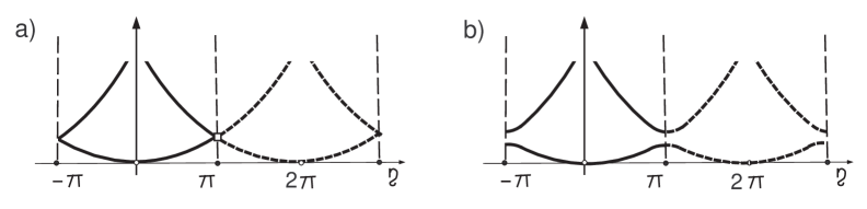
Figure 7: Duplication of the dispersion curves, limit a) and perturbed b).

Let us list the changes with respect to Section 6.1 which are necessary to support the asymptotic ansätze (6.4) and (6.5), (6.7) for the eigenpairs $\{\Lambda^{\varepsilon}_{p}(\eta),U^{\varepsilon}_{p}(x;\psi)\}$, $p=1,2$, of the problem (2.2)–(2.5) with the fast Floquet variable

$$\begin{array}[]{c}\displaystyle\psi=\varepsilon^{-1}(\eta-\pi)\end{array}$$ (6.43)

instead of (6.3).

To the eigenvalue $\Lambda^{0}:=\!\Lambda_{1}^{0}(\pi)\!=\!\Lambda_{2}^{0}(\pi)\!=\!\pi^{2}$ of the problem (2.12)–(2.14), there corresponds the eigenfunctions $U^{0}_{\pm}(x)=e^{\pm i\pi x_{1}}.$ Now, the main term in the outer expansion (6.5) becomes the linear combination of these eigenfunctions

$$\begin{array}[]{c}\displaystyle U^{0}(x_{1};\psi)=a_{+}(\psi)e^{+\pi ix_{1}}+a_{-}(\psi)e^{-\pi ix_{1}}.\end{array}$$

Notice that again no dependence on $x_{2}$ occurs. The main term in the inner expansion (6.7) keeps the form (6.8) but the correction terms look as follows:

$$\begin{array}[]{c}\displaystyle w^{\prime}(\xi;\psi)=\pi i(a_{+}(\psi)-a_{-}(\psi))W^{1}(\xi)+a^{\prime}(\psi)W^{0}\end{array}$$

and

$$\begin{array}[]{c}\displaystyle w^{\prime\prime}(\xi;\psi)=\pi^{2}(a_{+}(\psi)+a_{-}(\psi))W^{3}(\xi)+a^{\prime\prime}(\psi)W^{0}+\widetilde{w}^{\,\prime\prime}(\xi;\psi).\end{array}$$

Similarly to (6.11), (6.12), the jump conditions now read

$$\begin{array}[]{c}\displaystyle[U^{\prime}]_{0}(\psi)=2\pi i(a_{+}(\psi)-a_{-}(\psi))m_{1}(\Xi),\quad x_{2}\in(0,H),\\ \\ \displaystyle\Big{[}\frac{\partial U^{\prime}}{\partial x_{1}}\Big{]}_{0}(\psi)=\pi^{2}(a_{+}(\psi)+a_{-}(\psi))\frac{|\omega|}{H},\quad x_{2}\in(0,H).\end{array}$$ (6.44)

Moreover, instead of (6.14), we have

$$\begin{array}[]{c}e^{i\eta}=e^{i(\pi+\varepsilon\psi)}=e^{i\pi}(1+i\varepsilon\psi+O(\varepsilon^{2}))=-1-i\varepsilon\psi+O(\varepsilon^{2}),\end{array}$$

so that the somehow quasi-periodicity conditions of the type (6.15) turn into

$$\begin{array}[]{l}\displaystyle U^{\prime}\Big{(}\frac{1}{2},x_{2};\psi\Big{)}+U^{\prime}\Big{(}-\frac{1}{2},x_{2};\psi\Big{)}=-i\psi U^{0}\Big{(}-\frac{1}{2},x_{2};\psi\Big{)}=-\psi(a_{+}(\psi)-a_{-}(\psi)),\vspace{0.3cm}\\ \displaystyle\frac{\partial U^{\prime}}{\partial x_{1}}\Big{(}\frac{1}{2},x_{2};\psi\Big{)}+\frac{\partial U^{\prime}}{\partial x_{1}}\!\Big{(}-\frac{1}{2},x_{2};\psi\Big{)}=-i\psi\frac{\partial U^{0}}{\partial x_{1}}\Big{(}-\frac{1}{2},x_{2};\psi\Big{)}=-i\pi\psi\big{(}a_{+}(\psi)\!+\!a_{-}(\psi)\big{)}.\end{array}$$ (6.45)

It is worth mentioning that the relations (6.15) are nothing but inhomogeneous pure periodicity conditions while the relations (6.45) imply inhomogeneous anti-periodicity conditions of the function $U^{\prime}$.

The problem (6.13), (6.44), (6.45) with $\Lambda^{0}=\pi^{2}$ has two compatibility conditions which can be obtained by inserting the data of (6.45) and (6.44) into the Green formula as follows:

$$\begin{split}\Lambda^{\prime}(\psi)Ha_{\pm}(\psi)&=-\int\limits_{\varpi^{0}}\overline{e^{\pm\pi ix_{1}}}\left(\Delta U^{\prime}(x;\psi)+\Lambda^{0}U^{\prime}(x;\psi)\right)dx\\ &=-\int\limits_{0}^{H}e^{\mp\pi ix_{1}}\Big{(}\frac{\partial U^{\prime}}{\partial x_{1}}(x;\psi)\pm\pi iU^{\prime}(x;\psi)\Big{)}\bigg{|}_{-\frac{1}{2}}^{x_{1}=\frac{1}{2}}dx_{2}+\int\limits_{0}^{H}\Big{[}\frac{\partial U^{\prime}}{\partial x_{1}}(x;\psi)\pm\pi iU^{\prime}(x;\psi)\Big{]}_{0}\!dx_{2}.\end{split}$$

They convert into the system of two algebraic equations

$$\begin{array}[]{l}\displaystyle\Lambda^{\prime}(\psi)a_{+}(\psi)=\left(\!\pi^{2}\frac{|\omega|}{H}-2\pi^{2}m_{1}(\Xi)+2\pi\psi\right)a_{+}(\psi)+\left(\pi^{2}\frac{|\omega|}{H}+2\pi^{2}m_{1}(\Xi)\right)a_{-}(\psi),\vspace{0.3cm}\\ \displaystyle\Lambda^{\prime}(\psi)a_{-}(\psi)=\left(\pi^{2}\frac{|\omega|}{H}+2\pi^{2}m_{1}(\Xi)\right)a_{+}(\psi)+\left(\pi^{2}\frac{|\omega|}{H}-2\pi^{2}m_{1}(\Xi)-2\pi\psi\right)a_{-}(\psi),\end{array}$$ (6.46)

with the eigenvalues

$$\begin{array}[]{c}\displaystyle{\color[rgb]{0,0,0}\Lambda^{\prime}_{\pm}}(\psi)=2\pi\bigg{(}{\color[rgb]{0,0,0}\pi\Big{(}\frac{|\omega|}{2H}-m_{1}(\Xi)\Big{)}}\pm\sqrt{\pi^{2}\Big{(}m_{1}(\Xi){\color[rgb]{0,0,0}+}\frac{|\omega|}{2H}\Big{)}^{2}+\psi^{2}}\bigg{)},\end{array}$$ (6.47)

where

$$\Lambda^{\prime}_{-}(\psi)\leq-4\pi^{2}m_{1}(\Xi)\,\,\hbox{ and }\,\,\Lambda^{\prime}_{+}(\psi)\geq 2\pi^{2}\frac{|\omega|}{H}.$$ (6.48)

The corresponding $a^{\pm}(\psi)=(a^{\pm}_{+}(\psi),a^{\pm}_{-}(\psi))$ can be easily computed from the algebraic equations (6.46). We again have $\Lambda^{\prime}_{+}(\psi)>\Lambda^{\prime}_{-}(\psi)$ and therefore, we establish the relation of the eigenpairs $\{\Lambda^{\prime}_{-}(\psi),a^{-}(\psi)\}$ and $\{\Lambda^{\prime}_{+}(\psi),a^{+}(\psi)\}$, respectively, with the eigenpairs $\{\Lambda^{\varepsilon}_{1}(\eta),U^{\varepsilon}_{1}(x;\psi)\}$ and $\{\Lambda^{\varepsilon}_{2}(\eta),U^{\varepsilon}_{2}(x;\psi)\}$ of the problem (2.2)–(2.5) with $\eta$ defined by (6.43).

Now, we formulate our result on splitting edges of the first and second limit spectral bands giving rise to the open gap $\gamma_{1}^{\varepsilon}$ (cf. Figure 5 a) and b)); here, we take into account the $2\pi-$periodicity in $\eta$ of the functions $\Lambda_{p}^{\varepsilon}(\eta)$.

Theorem 6.3.

Let $H\in(0,1)$ and $\psi_{1}>0$. Then, there exist positive $\varepsilon_{0}=\varepsilon_{0}(H,\psi_{1})$ and $C=C(H,\psi_{1})$ such that, for $\varepsilon\in(0,\varepsilon_{0}]$, the entries $\Lambda^{\varepsilon}_{1}(\eta)$ and $\Lambda^{\varepsilon}_{2}(\eta)$ of the eigenvalue sequence (2.7) with $\eta=\pi+\varepsilon\psi$, $|\psi|\leq\psi_{1}$, meet the estimates

$$\begin{array}[]{c}\displaystyle|\Lambda^{\varepsilon}_{2}({\color[rgb]{0,0,0}\pi+}\varepsilon\psi)-\pi^{2}-\varepsilon{\color[rgb]{0,0,0}\Lambda_{+}^{\prime}}(\psi)|\leq{\color[rgb]{0,0,0}C\varepsilon^{2}},\vspace{0.2cm}\\ |\Lambda^{\varepsilon}_{1}({\color[rgb]{0,0,0}\pi+}\varepsilon\psi)-\pi^{2}-\varepsilon{\color[rgb]{0,0,0}\Lambda_{-}^{\prime}}(\psi)|\leq{\color[rgb]{0,0,0}C\varepsilon^{2}},\end{array}$$

where the quantities ${\color[rgb]{0,0,0}\Lambda_{\pm}^{\prime}}(\psi)$ are given by (6.47).

7  Opening the spectral gaps

In this section, we show that, under the mirror symmetry condition of the holes, cf. (1.9), there are open spectral gaps for the spectrum (1.7) of the original problem (1.4)–(1.5) in the perforated waveguide $\Pi^{\varepsilon}$, cf. (1.3); see also Figures 1 and 2. Further specifying, for the values $H\in(0,1)$ we show that there is at least one open gap while for $H\in(0,1/2)$ there are at least two open gaps. We provide asymptotic formulas for their localization and width, cf. Figure 5 b) and a) respectively and formulas (7.1)–(7.3), (7.6) and (7.7). In Sections 7.1 and 7.2, respectively, we broach the cases where $H\in(0,1)$ and $H\in(0,1/2)$.

7.1  Opening spectral gap near the node $(\eta_{\mbox{\tiny$\square$}},\Lambda_{\mbox{\tiny$\square$}})$

Recall $(\eta_{\mbox{\tiny$\square$}},\Lambda_{\mbox{\tiny$\square$}})=(\pm\pi,\pi^{2})$. Based on asymptotic formulas in Theorems 5.1 and 6.3, we prove in this section that

$$\begin{array}[]{c}\displaystyle\max\limits_{\eta\in[-\pi,\pi]}\Lambda^{\varepsilon}_{1}(\eta)\leq\pi^{2}-4\pi^{2}\varepsilon m_{1}(\Xi)+O(\varepsilon^{2}),\vspace{0.2cm}\\ \displaystyle\min_{\eta\in[-\pi,\pi]}\Lambda^{\varepsilon}_{2}(\eta)\geq\pi^{2}+2\pi^{2}\varepsilon\frac{|\omega|}{H}+O(\varepsilon^{2}).\end{array}$$ (7.1)

In this way, since $m_{1}(\Xi)\pm(2H)^{-1}|\omega|>0$ (see Proposition 3.3), the spectral gap

$$\begin{array}[]{c}\displaystyle\gamma^{\varepsilon}_{p}=(\max_{\eta}\Lambda^{\varepsilon}_{p}(\eta),\min_{\eta}\Lambda^{\varepsilon}_{p+1}(\eta))\end{array}$$ (7.2)

with $p=1$ stays open and has the width

$$\begin{array}[]{c}\displaystyle|\gamma^{\varepsilon}_{1}|\geq 4\pi^{2}\varepsilon\Big{(}m_{1}(\Xi)+\frac{|\omega|}{2H}\Big{)}+O(\varepsilon^{2}).\end{array}$$ (7.3)

Let us prove (7.1) for $H\in(0,1)$. We divide the proof in two parts depending on whether $\eta\in I_{1}$ or $\eta\in I_{2}$ where the sets $I_{1}=[-\pi+\delta_{1},\pi-\delta_{1}]$ and $I_{2}=[-\pi,-\pi+\delta_{1}]\cup[\pi-\delta_{1},\pi]$ for certain $\delta_{1}\in(0,\pi)$, cf. Figure 8. For simplicity, we choose $\delta_{1}$ such that $\Lambda_{-}^{0}(\pi-\delta_{1})=(\pi+\delta_{1})^{2}<\pi^{2}+K_{2}$ where $K_{2}$ is defined by (2.31). Thus, by Proposition 2.3, we have that there exists $\varepsilon_{1}=\varepsilon(H,\delta_{1})>0$ such that

$$\Lambda_{2}^{\varepsilon}(\eta)>\pi^{2}+K_{1}\qquad \mbox{for }\eta\in I_{1},\,\varepsilon<\varepsilon_{1},$$ (7.4)

$$\Lambda_{3}^{\varepsilon}(\eta)>\pi^{2}+K_{2}\qquad \mbox{for }\eta\in I_{2},\,\varepsilon<\varepsilon_{1},$$ (7.5)

where $K_{1}$ and $K_{2}$ are defined by (2.31) and $K_{1}$ may depend on $\delta_{1}$. In addition, when $\eta\in I_{2}$, we separate again into two parts $\eta\in I_{2}\cap\{\eta\,:\,\pi-|\eta|\leq\varepsilon\psi_{1}\}$ and $\eta\in I_{2}\cap\{\eta\,:\,\pi-|\eta|\geq\varepsilon\psi_{1}\}$ for a certain constant $\psi_{1}>0$ that we will determine below.

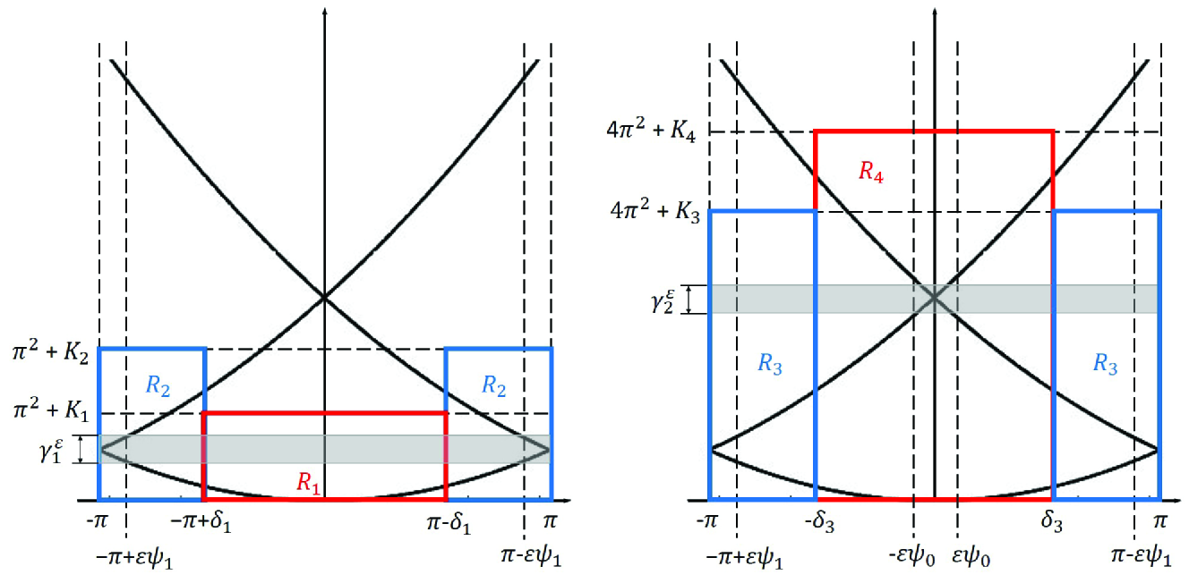
Figure 8: The different boxes $R_{p}$ for $p=1,2,3,4.$

Firstly, we estimate $\Lambda_{1}^{\varepsilon}(\eta)$ and $\Lambda_{2}^{\varepsilon}(\eta)$ for $\eta\in I_{1}$ where (7.4) holds, namely, the case where, for $\varepsilon$ small enough, there cannot be more than one eigenvalue $\Lambda_{p}^{\varepsilon}(\eta)$ in the box $R_{1}:=I_{1}\times[0,\pi^{2}+K_{1}].$ Thus, it is evident that

$$\Lambda^{\varepsilon}_{2}(\eta)\geq\pi^{2}+2\pi^{2}\varepsilon\frac{|\omega|}{H}+O(\varepsilon^{2})\quad\mbox{for }\eta\in I_{1}.$$

Besides, by Corollary 5.2, we have

$$\Lambda^{\varepsilon}_{1}(\eta)\leq\Lambda_{1}^{0}(\eta)+C_{0}\varepsilon\leq(\pi-\delta_{1})^{2}+C_{0}\varepsilon\leq\pi^{2}-4\pi^{2}m_{1}(\Xi)\varepsilon\quad\mbox{for }\eta\in I_{1}$$

and $\varepsilon$ small enough, which concludes the proof in $I_{1}.$

Secondly, we estimate $\Lambda_{1}^{\varepsilon}(\eta)$ and $\Lambda_{2}^{\varepsilon}(\eta)$ for $\eta\in I_{2}$ where (7.5) holds, namely, the case where, for $\varepsilon$ small enough, there cannot be more than two eigenvalues $\Lambda_{p}^{\varepsilon}(\eta)$ in the boxes $R_{2}:=I_{2}\times[0,\pi^{2}+K_{2}].$ Now, for any $\psi_{1}>0$, Theorem 6.3 and (6.48) allow us to obtain, for $\varepsilon$ small enough, the extremum in (7.1) restricted to $\eta\in I_{2}\cap\{\eta\,:\,\pi-|\eta|\leq\varepsilon\psi_{1}\}$. Moreover, for $C_{0}$ the constant arising in (5.1) and (5.2), fixing

$$\psi_{1}>C_{0}/2\pi,$$

we observe that the eigenvalues $\Lambda_{\star}^{\varepsilon}(\eta),\,\Lambda_{-}^{\varepsilon}(\eta)$ defined by Theorem 5.1 satisfy

$$\Lambda_{-}^{\varepsilon}(\eta)-\Lambda_{\star}^{\varepsilon}(\eta)\!\geq\!\Lambda_{-}^{0}(\eta)-\Lambda_{1}^{0}(\eta)-2C_{0}\varepsilon\!=\!4\pi(\pi-\eta)-2C_{0}\varepsilon>0\,\,$$

for $\eta>0,\pi-\eta\geq\varepsilon\psi_{1},$ and $\Lambda_{-}^{\varepsilon}(\eta)\leq\Lambda_{-}^{0}(\eta)+C_{0}\varepsilon\leq\Lambda_{-}^{0}(\pi-\delta_{1})+C_{0}\varepsilon\leq\pi^{2}+K_{2}$ for $\eta\in[\pi-\delta_{1},\pi]$ and $\varepsilon$ small enough. As a consequence, we can identify $\Lambda_{1}^{\varepsilon}(\eta)=\Lambda_{\star}^{\varepsilon}(\eta)$ and $\Lambda_{2}^{\varepsilon}(\eta)=\Lambda_{-}^{\varepsilon}(\eta)$ for $\eta\in[\pi-\delta_{1},\pi-\varepsilon\psi_{1}]$, cf. (7.5). Thus, using Theorem 5.1 and taking

$$\psi_{1}=\max\left\{\frac{4\pi^{2}m_{1}(\Xi)+C_{0}}{\pi},\frac{C_{0}H+2\pi^{2}|\omega|}{2\pi H}\right\},$$

for $\varepsilon$ small enough, we have

$$\begin{split}\Lambda^{\varepsilon}_{1}(\eta)&\leq\Lambda_{1}^{0}(\eta)+C_{0}\varepsilon=\pi^{2}-(\pi+\eta)(\pi-\eta)+C_{0}\varepsilon\vspace{0.1cm}\\ &\leq\pi^{2}-\pi(\pi-\eta)+C_{0}\varepsilon\leq\pi^{2}-4\pi^{2}m_{1}(\Xi)\varepsilon\qquad\mbox{for }\eta\in[\pi-\delta_{1},\pi-\varepsilon\psi_{1}],\vspace{0.2cm}\\ \Lambda^{\varepsilon}_{2}(\eta)&\geq\Lambda_{-}^{0}(\eta)-C_{0}\varepsilon=\pi^{2}+(3\pi-\eta)(\pi-\eta)-C_{0}\varepsilon\\ &\geq\pi^{2}+2\pi(\pi-\eta)-C_{0}\varepsilon\geq\pi^{2}+2\pi^{2}\frac{|\omega|}{H}\varepsilon\qquad\mbox{for }\eta\in[\pi-\delta_{1},\pi-\varepsilon\psi_{1}].\end{split}$$

In a similar way, we can estimate $\Lambda_{1}^{\varepsilon}(\eta)$ and $\Lambda_{2}^{\varepsilon}(\eta)$ for $\eta\in[-\pi+\varepsilon\psi_{1},-\pi+\delta_{1}],$ where now $\Lambda_{1}^{\varepsilon}(\eta)=\Lambda_{\star}^{\varepsilon}(\eta)$ and $\Lambda_{2}^{\varepsilon}(\eta)=\Lambda_{+}^{\varepsilon}(\eta)$. This concludes the proof for $\eta\in I_{2}.$

Now we formulate our result on opening spectral gap $\gamma^{\varepsilon}_{1}$ (see Figure 5 a)–b)):

Theorem 7.1.

Let $H\in(0,1)$. Then, there exists a positive constant $\varepsilon_{0}=\varepsilon_{0}(H)$ such that, for $\varepsilon\in(0,\varepsilon_{0}]$, the asymptotic formulas (7.1) are valid and the gap (7.2) with $p=1$ has positive length (7.3).

7.2  Opening spectral gap near the node $(\eta_{\mbox{\small{$\circ$}}},\Lambda_{\mbox{\small{$\circ$}}})$

Recall $(\eta_{\mbox{\small{$\circ$}}},\Lambda_{\mbox{\small{$\circ$}}})=(0,4\pi^{2})$. Similar computations on the base of Theorems 5.1, 6.1 and 6.3 prove that

$$\begin{array}[]{c}\displaystyle\max_{\eta\in[-\pi,\pi]}\Lambda^{\varepsilon}_{2}(\eta)\leq 4\pi^{2}-16\pi^{2}\varepsilon m_{1}(\Xi)+O(\varepsilon^{2}),\\ \displaystyle\min_{\eta\in[-\pi,\pi]}\Lambda^{\varepsilon}_{3}(\eta)\geq 4\pi^{2}+8\pi^{2}\varepsilon\frac{|\omega|}{H}+O(\varepsilon^{2}),\end{array}$$ (7.6)

so that the gap (7.2) with $p=2$ opens and gets the width

$$\begin{array}[]{c}\displaystyle|\gamma^{\varepsilon}_{2}|\geq 16\pi^{2}\varepsilon\Big{(}m_{1}(\Xi)+\frac{|\omega|}{2H}\Big{)}+O(\varepsilon^{2}).\end{array}$$ (7.7)

Let us prove (7.6) for $H\in(0,1/2)$. Now, we divide the proof in two parts depending on whether $\eta\in I_{3}$ or $\eta\in I_{4}$ where the sets $I_{3}=[-\pi,-\delta_{3}]\cup[\delta_{3},\pi]$ and $I_{4}=[-\delta_{3},\delta_{3}]$ for certain $\delta_{3}\in(0,\pi)$, cf. Figure 8. For simplicity, we choose $\delta_{3}$ such that $\Lambda_{+}^{0}(\delta_{3})=(2\pi+\delta_{3})^{2}<4\pi^{2}+K_{4}$ where $K_{4}$ is defined by (2.35). Thus, by Proposition 2.4 we have that there exists $\varepsilon_{1}=\varepsilon(H,\delta_{3})>0$ such that

$$\Lambda_{3}^{\varepsilon}(\eta)>4\pi^{2}+K_{3}\qquad \mbox{for }\eta\in I_{3},\,\varepsilon<\varepsilon_{1},$$ (7.8)

$$\Lambda_{4}^{\varepsilon}(\eta)>4\pi^{2}+K_{4}\qquad \mbox{for }\eta\in I_{4},\,\varepsilon<\varepsilon_{1},$$ (7.9)

where $K_{3}$ and $K_{4}$ are defined by (2.35) and $K_{3}$ may depend on $\delta_{3}$. In addition, when $\eta\in I_{3}$ or $\eta\in I_{4}$, we separate again into two parts, namely, we distinguish the four cases $\eta\in I_{3}\cap\{\eta\,:\,\pi-|\eta|\leq\varepsilon\psi_{1}\}$, $\eta\in I_{3}\cap\{\eta\,:\,\pi-|\eta|\geq\varepsilon\psi_{1}\}$, $\eta\in[-\varepsilon\psi_{0},\varepsilon\psi_{0}]\subset I_{4}$ and $\eta\in I_{4}\cap\{\eta\,:\,|\eta|\geq\varepsilon\psi_{0}\}$ for a certain $\psi_{0},\psi_{1}>0$.

Firstly, we estimate $\Lambda_{2}^{\varepsilon}(\eta)$ and $\Lambda_{3}^{\varepsilon}(\eta)$ for $\eta\in I_{3}$ where (7.8) holds, namely, the case where, for $\varepsilon$ small enough, there cannot be more than two eigenvalues $\Lambda_{p}^{\varepsilon}(\eta)$ in the boxes $R_{3}:=I_{3}\times[0,4\pi^{2}+K_{3}].$ Thus, it is evident that

$$\Lambda^{\varepsilon}_{3}(\eta)\geq 4\pi^{2}+8\pi^{2}\varepsilon\frac{|\omega|}{H}+O(\varepsilon^{2})\quad\mbox{for }\eta\in I_{3}=[-\pi,-\delta_{3}]\cup[\delta_{3},\pi].$$

Besides, for any $\psi_{1}>0$, by virtue of Theorem 6.3 and (6.47), we get that

$$\Lambda_{2}^{\varepsilon}(\eta)\leq\pi^{2}+K(\psi_{1})\varepsilon<2\pi^{2}\qquad\mbox{for }\eta\in I_{3}\cap\{\eta\,:\,\pi-|\eta|\leq\varepsilon\psi_{1}\}$$

and $\varepsilon$ small enough. Now, fixing $\psi_{1}>C_{0}/2$ and repeating the arguments in the previous Section 7.1 related with the set $I_{2}$, we can identify $\Lambda_{2}^{\varepsilon}(\eta)=\Lambda_{-}^{\varepsilon}(\eta)$ for $\eta\in[\delta_{3},\pi-\varepsilon\psi_{1}]$ and $\Lambda_{2}^{\varepsilon}(\eta)=\Lambda_{+}^{\varepsilon}(\eta)$ for $\eta\in[-\pi+\varepsilon\psi_{1},-\delta_{3}].$ Thus, by virtue of Theorem 5.1, we can check that

$$\Lambda^{\varepsilon}_{2}(\eta)\leq 4\pi^{2}-16\pi^{2}\varepsilon m_{1}(\Xi)+O(\varepsilon^{2})\quad\mbox{for }\eta\in I_{3}\cap\{\eta\,:\,\pi-|\eta|\geq\varepsilon\psi_{1}\}.$$

and $\varepsilon$ small enough. This concludes the proof on the interval $I_{3}.$

Secondly, we estimate $\Lambda_{2}^{\varepsilon}(\eta)$ and $\Lambda_{3}^{\varepsilon}(\eta)$ when $\eta\in I_{4}$ where (7.9) holds, namely, the case where, for $\varepsilon$ small enough, there cannot be more than three eigenvalues $\Lambda_{p}^{\varepsilon}(\eta)$ in the box $R_{4}:=I_{4}\times[0,4\pi^{2}+K_{4}].$ Now, for any $\psi_{0}>0$, Theorem 6.1 and (6.19) allow us to obtain, for $\varepsilon$ small enough, the extremum in (7.6) restricted to $\{\eta=\varepsilon\psi\,:\,|\psi|\leq\psi_{0}\}.$ Moreover, fixing $\psi_{0}>C_{0}/4\pi$, we observe that the eigenvalues $\Lambda_{\pm}^{\varepsilon}(\eta)$ defined by Theorem 5.1 satisfy

$$\Lambda_{+}^{\varepsilon}(\eta)-\Lambda_{-}^{\varepsilon}(\eta)\geq\Lambda_{+}^{0}(\eta)-\Lambda_{-}^{0}(\eta)-2C_{0}\varepsilon=8\pi\eta-2C_{0}\varepsilon>0\quad\mbox{for }\eta\geq\varepsilon\psi_{0},$$

and $\Lambda_{+}^{\varepsilon}(\eta)\leq\Lambda_{+}^{0}(\eta)+C_{0}\varepsilon\leq\Lambda_{+}^{0}(\delta_{3})+C_{0}\varepsilon\leq 4\pi^{2}+K_{4}$, for $\eta\in[0,\delta_{3}]$ and $\varepsilon$ small enough. As a consequence, we can identify $\Lambda_{2}^{\varepsilon}(\eta)=\Lambda_{-}^{\varepsilon}(\eta)$ and $\Lambda_{3}^{\varepsilon}(\eta)=\Lambda_{+}^{\varepsilon}(\eta)$ for $\eta\in[\varepsilon\psi_{0},\delta_{3}].$ Note that, by Corollary 5.2, $\Lambda_{1}^{\varepsilon}(\eta)=\Lambda_{\star}^{\varepsilon}(\eta)$ for $\eta\in[-\delta_{3},\delta_{3}]$ and there cannot be more than three eigenvalues $\Lambda_{p}^{\varepsilon}(\eta)$ in the box $I_{4}\times[0,4\pi^{2}+K_{4}].$ Thus, using again Theorem 5.1 and taking

$$\psi_{0}=\max\left\{\frac{16\pi^{2}m_{1}(\Xi)+C_{0}}{3\pi},\frac{C_{0}H+8\pi^{2}|\omega|}{4\pi H}\right\},$$

for $\varepsilon$ small enough, we have

$$\begin{split}\Lambda^{\varepsilon}_{2}(\eta)&\leq\Lambda_{-}^{0}(\eta)+C_{0}\varepsilon=4\pi^{2}-(4\pi-\eta)\eta+C_{0}\varepsilon\leq 4\pi^{2}-3\pi\eta+C_{0}\varepsilon\vspace{0.15cm}\\ &\leq 4\pi^{2}-16\pi^{2}m_{1}(\Xi)\varepsilon\qquad\mbox{for }\eta\in[\varepsilon\psi_{0},\delta_{3}],\vspace{0.3cm}\\ \Lambda^{\varepsilon}_{3}(\eta)&\geq\Lambda_{+}^{0}(\eta)-C_{0}\varepsilon=4\pi^{2}+(4\pi+\eta)\eta-C_{0}\varepsilon\geq 4\pi^{2}+4\pi\eta-C_{0}\varepsilon\\ &\geq 4\pi^{2}+8\pi^{2}\frac{|\omega|}{H}\varepsilon\qquad\mbox{for }\eta\in[\varepsilon\psi_{0},\delta_{3}].\end{split}$$

In a similar way, we can estimate $\Lambda_{2}^{\varepsilon}(\eta)$ and $\Lambda_{3}^{\varepsilon}(\eta)$ for $\eta\in[-\delta_{3},-\varepsilon\psi_{0}],$ where now $\Lambda_{2}^{\varepsilon}(\eta)=\Lambda_{+}^{\varepsilon}(\eta)$ and $\Lambda_{3}^{\varepsilon}(\eta)=\Lambda_{-}^{\varepsilon}(\eta)$. This concludes the proof for $\eta\in I_{4}.$

Now we formulate our result on opening spectral gap $\gamma^{\varepsilon}_{2}$ (see Figure 5 a)):

Theorem 7.2.

Let $H\in(0,1/2)$. Then, there exists a positive constant $\varepsilon_{0}=\varepsilon_{0}(H)$ such that, for $\varepsilon\in(0,\varepsilon_{0}]$, the asymptotic formulas (7.6) are valid and the gap (7.2) with $p=2$ has positive length (7.7).

8  Concluding remarks and open problems

We comment on other possible spectral gaps arising from other nodes of the limit dispersion curves which are not considered in previous sections.

8.1  Closed and shaded gaps

We note that the nodes marked with $\bullet$ and $\blacksquare$ in Figure 4 a)–c), can separate when dealing with the perturbed problem, but do not give rise to spectral gaps because they are shaded by other dispersion curves in Figure 5 a)–c). More precisely, the node $(0,4\pi^{2})$ marked with $\circ$ in Figure 4 a) gets the symbol $\bullet$ in Figure 4 b) and c) because the spectral gap described in Theorem 7.2 is shaded by a small perturbation, see Section 4, of the limit dispersion curves

$$\Lambda=\frac{\pi^{2}}{H^{2}}+\eta^{2},\,\,\eta\in[-\pi,\pi],\quad\mbox{\rm for}\,\,H\in\Big{(}\frac{1}{2},\frac{1}{\sqrt{3}}\Big{)},$$

$$\Lambda=\frac{\pi^{2}}{H^{2}}+(\eta\mp 2\pi)^{2},\,\,\pm\eta\in[0,\pi],\quad\mbox{\rm for}\,\,H>\frac{1}{\sqrt{3}}.$$

In a similar way, after perturbation, the node $(\pm\pi,\pi^{2})$, marked with $\square$ in Figure 4 a) and b) provides an open spectral gap when $H\in(0,1)$ but the same node in Figure 4 c) is marked with $\blacksquare$ because the gap around it is shaded by a small perturbation of the dispersion curve

$$\Lambda=\frac{\pi^{2}}{H^{2}}+\eta^{2},\,\,\eta\in[-\pi,\pi],\quad\mbox{\rm for}\,\,H>1.$$

Other nodes such as $(\eta_{\mbox{\small$\bullet$}},\Lambda_{\mbox{\small$\bullet$}})=(0,\pi^{2}H^{-2})$ and $(\eta_{\mbox{\tiny$\blacksquare$}},\Lambda_{\mbox{\tiny$\blacksquare$}})=(\pm\pi,\pi^{2}(1+H^{-2}))$, also detected in Figure 4 a)–c), do not give rise to open spectral gaps with some possible exceptions: $H=1$, $H=1/\sqrt{3}$, $H=1/2$, $H=1/\sqrt{5}$, $H=1/\sqrt{8}$ and others (cf. Figures 3 and 9). To examine these nodes in these exceptional cases, important modifications of our calculations in Section 6.1 and 6.4 are needed and we postpone their study.

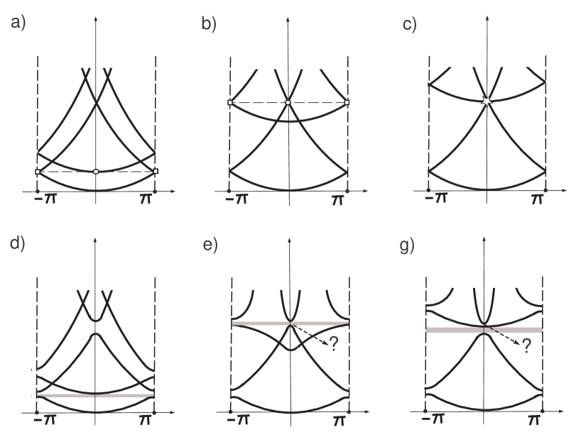
Figure 9: The exceptional cases $H=1$, $H=1/\sqrt{3}$ and $H=1/2$.

The nodes marked with $\blacktriangleleft$ and $\blacktriangleright$ in Figure 4 a), do not give rise to open gaps due to another reason as depicted schematically in Figure 10: both cases of perturbed curves do not provide a gap. A rigorous justification of the absence of spectral gaps around nodes generated by similar, either ascending, or descending, dispersion curves can be found in [31].

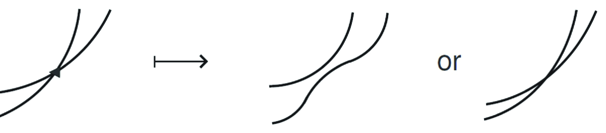
Figure 10: The perturbation of ascending curves.

8.2  On the symmetry assumption and possible generalizations

Under the symmetry assumption (1.9) we reduce the problem (2.2)–(2.5) to the lower half of the periodicity cell (1.8)

$$\begin{array}[]{c}\displaystyle-\Delta U^{\varepsilon}(x;\eta)=\Lambda^{\varepsilon}(\eta)U^{\varepsilon}(x;\eta),\quad x\in\{x\in\varpi^{\varepsilon}:\,x_{2}<H/2\},\vspace{0.2cm}\\ \displaystyle U^{\varepsilon}\Big{(}\frac{1}{2},x_{2};\eta\Big{)}=e^{i\eta}U^{\varepsilon}\Big{(}-\frac{1}{2},x_{2};\eta\Big{)},\quad x_{2}\in\Big{(}0,\frac{H}{2}\Big{)},\vspace{0.3cm}\\ \displaystyle\frac{\partial U^{\varepsilon}}{\partial x_{1}}\Big{(}\frac{1}{2},x_{2};\eta\Big{)}=e^{i\eta}\frac{\partial U^{\varepsilon}}{\partial x_{1}}\Big{(}-\frac{1}{2},x_{2};\eta\Big{)},\quad x_{2}\in\Big{(}0,\frac{H}{2}\Big{)},\vspace{0.3cm}\\ \displaystyle\partial_{\nu}U^{\varepsilon}(x)=0,\quad x\in\{x\in\partial\varpi^{\varepsilon}:\,|x_{1}|<1/2,\,\,x_{2}<H/2\}.\end{array}$$ (8.1)

On the truncation line $\Sigma^{\varepsilon}=\{x\in\varpi^{\varepsilon}:\,x_{2}=H/2\}$, we impose an artificial boundary condition, either the Neumann condition

$$\begin{array}[]{c}\displaystyle\frac{\partial U^{\varepsilon}}{\partial x_{2}}(x;\eta)=0,\,\,x\in\Sigma^{\varepsilon},\end{array}$$ (8.2)

or the Dirichlet one

$$\begin{array}[]{c}U^{\varepsilon}(x;\eta)=0,\,\,x\in\Sigma^{\varepsilon}.\end{array}$$ (8.3)

Clearly, in view of the geometrical symmetry the even (in the variable $x_{2}-H/2$) extension above $\Sigma^{\varepsilon}$ of an eigenfunction of the problem (8.1), (8.2) becomes an eigenfunction of the problem (2.2)–(2.5) with the same eigenvalue while the odd extension does the same with an eigenfunction of the problem (8.1), (8.3)

A similar reduction of the limit problem (2.12)–(2.14) divides the family (2.15) of eigenpairs into two groups containing even ($q=2j$) and odd ($q=1+2j$) in the variable $x_{2}-H/2$ eigenfunctions (2.15). Hence, the eigenfunctions in the first and second groups satisfy the Neumann and Dirichlet artificial boundary conditions on the horizontal mid-line $\{x\in\Pi^{\varepsilon}:\,x_{2}=H/2\}$ of the perforated strip $\Pi^{\varepsilon}$. The limit dispersion curves are drawn in Figure 11 a) and b), respectively. The previous asymptotic analysis applied to problems (8.1), (8.3) and (8.1), (8.2) independently leads to the dispersion curves in Figure 11 c) and d), respectively. Furthermore, the common graph in Figure 5 b) is obtained by uniting the latter graphs after perturbations so that the nodes $\lozenge$ in Figure 4 b) do not separate in contrast to the nodes marked with $\square$ and $\circ$ (see Figure 12). We recognize this fact as the lack of interaction between the intersecting curves (6.1) with the index couples $(j,k)=(\pm 1,0)$ and $(j,k)=(0,1)$ in (2.15).

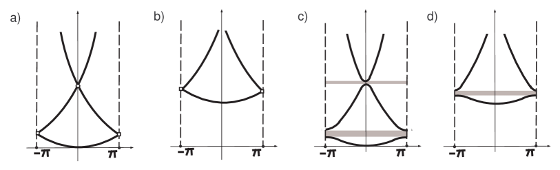
Figure 11: Disjoint trusses under the symmetry condition.

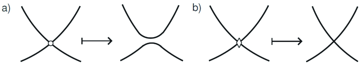
Figure 12: The perturbation of similar and dissimilar curves.

As depicted in Figure 5 b)–c), all nodes marked with $\lozenge$ in Figure 4 do not split due to the geometrical symmetry (1.9). One may hope that denying the symmetry assumption (1.9) provides separation of the nodes $\lozenge$ to open many gaps in Figure 6 a)–c). However, we cannot confirm such a splitting of band edges by our present asymptotic analysis.

Another way to conclude on splitting by analyzing the first correction term in the eigenvalue asymptotics only is to treat either inclined perforation springs, Figure 13 a) or holes of varying size, Figure 13 b). Again both modifications require a serious complication of calculations.

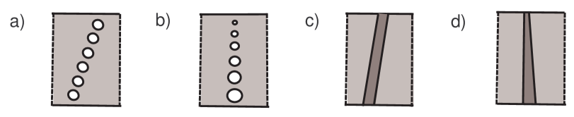
Figure 13: The distorted periodicity cells.

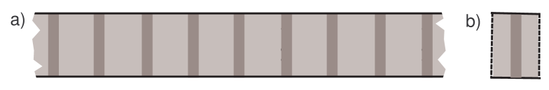
Figure 14: The waveguide with periodic strata.

A similar spectral problem in a stratified strip in Figure 14 a) with foreign acoustic material in shaded thin rectangles can be solved explicitly by separating variables. However, in the case of straight and homogeneous strata as in Figure 14 b), we again cannot conclude on the splitting of the nodes $\lozenge$ while dealing with the first correction term only. To clarify the possibility of opening corresponding spectral gaps, one can disturb the strata as depicted in Figure 13 c) and d), or even deal with curved stratum in the periodicity cell, namely

$$\begin{array}[]{c}\varsigma^{\varepsilon}=\{x:\,x_{2}\in(0,H),\,-\varepsilon h_{-}(x_{2})<x_{1}-j<\varepsilon h_{+}(x_{2})\},\end{array}$$

where $h\pm\in C^{\infty}[0,H]$ are profile functions such that

$$\begin{array}[]{c}h(x_{2})=h_{+}(x_{2})+h_{-}(x_{2})>0,\,\,x_{2}\in[0,H].\end{array}$$

However, this perturbation on the thin strips and those outlined in Figure 13 stay as open problems. A study of the corresponding spectrum will be undertaken in the forthcoming paper of the authors.

References

- [1] G. Allaire and C. Conca, Bloch wave homogenization and spectral asymptotic analysis, J. Math. Pures Appl. 77 (1998) 153–208.
- [2] H. Attouch, Variational Convergence for Functions and Operators. Applicable Mathematics Series, Pitman, Boston, 1984.
- [3] F.L. Bakharev, G. Cardone, S.A. Nazarov and J. Taskinen, Effects of Rayleigh waves on the essential spectrum in perturbed doubly periodic elliptic problems, Integral Equations Operator Theory 88 (2017) 373–386.
- [4] F.L. Bakharev and S.A. Nazarov, Gaps in the spectrum of a waveguide composed of domains with different limiting dimensions, Sibirsk. Mat. Zh. 56 (2015) 732–751 (English transl.: Sib. Math. J. 56 (2015) 575–592).
- [5] F.L. Bakharev, S.A. Nazarov and K.M. Ruotsalainen, A gap in the spectrum of the Neumann-Laplacian on a periodic waveguide, Appl. Anal. 92 (2013) 1889–1995.
- [6] F.L. Bakharev and E. Pérez, Spectral gaps for the Dirichlet-Laplacian in a 3-D waveguide periodically perturbed by a family of concentrated masses, Math. Nachr. 291 (2018) 556–575.
- [7] F.L. Bakharev and J. Taskinen, Bands in the spectrum of a periodic elastic waveguide, Z. Angew. Math. Phys. 68 (2017) paper 122, 27pp.
- [8] A. Bensoussan, J.-L. Lions and G. Papanicolau, Asymptotic Analysis for Periodic Structures, North-Holland Publishing Co., Amsterdam, 1978.
- [9] M.S. Birman and M.Z. Solomyak, Spectral Theory and SelfAdjoint Operators in Hilbert Space, Reidel Publishing Co., Dordrecht, 1987.
- [10] D.I. Borisov and K.V. Pankrashkin, Gap opening and split band edges in waveguides coupled by a periodic system of small windows, Mat. Zametki 93 (2013) 665–683 (English transl.: Math. Notes 93 (2013) 660–675).
- [11] D.I. Borisov and K.V. Pankrashkin, Quantum waveguides with small periodic perturbations: gaps and edges of Brillouin zones, J. Phys. A 46 (2013) e235203, 18 pp.
- [12] C. Conca, J. Planchard and M. Vanninathan, Fluids and Periodic Structures. Masson, Paris, 1995.
- [13] I.M. Gelfand, Expansions in characteristic functions of an equation with periodic coefficients [in Russian], Doklady Akad. Nauk. SSSR 73 (1950) 1117–1120.
- [14] D. Gómez, S.A. Nazarov, R. Orive-Illera and M.-E. Pérez-Martínez, Remark on justification of asymptotics of spectra of cylindrical waveguides with periodic singular perturbations of boundary and coefficients, J. Math. Sci. 257 (2021) 597–623 (translated from Russian: Problemy Matematicheskogo Analiza 111 (2021) 43–65).
- [15] R. Hempel and K Lienau, Spectral properties of periodic media in the large coupling limit, Comm. Partial Differential Equations 25 (2000) 1445–1470.
- [16] R. Hempel and O. Post, Spectral gaps for periodic elliptic operators with high contrast: an overview, in: Progress in Analysis, Proceedings of the 3rd International ISAAC Congress Berlin 2001, World Scientific Publ., River Edge, NJ, pp. 577–587, 2003.
- [17] A.M. Il’in, Matching of Asymptotic Expansions of Solutions of Boundary Value Problems, Am. Math. Soc., Providence, RI 1992.
- [18] P. Kuchment, Floquet Theory for Partial Differential Equations, Birkhäuser Verlag, Basel, 1993.
- [19] O.A. Ladyzhenskaya, The Mathematical Theory of Viscous Incompressible Flow, 2nd ed., Nauka, Moscow 1970, 288 pp.; (English transl., 2nd Eng. ed., rev. and enlarged, Math. Appl., vol. 2, Gordon and Breach Science Publishers, New York-London-Paris 1969, xviii+224 pp.).
- [20] M. Lobo, O.A. Oleinik, M.E. Pérez and T.A. Shaposhnikova, On homogenization of solutions of boundary value problems in domains, perforated along manifolds. Ann. Scuola Norm. Sup. Pisa Cl. Sci. 4e série, 25 (1997) 611–629.
- [21] V.G. Maz’ya, S.A. Nazarov and B.A. Plamenevsky, Asymptotic Theory of Elliptic Boundary Value Problems in Singularly Perturbed Domains Vols. 1 & 2, Birkhäuser Verlag, Basel, 2000.
- [22] V.A. Marchenko and E.Ya. Khruslov, Boundary Value Problems in Domains with a Fine-Grained Boundary, Naukova Dumka, Kiev, 1974 (in Russian).
- [23] S.A. Nazarov, Asymptotic behavior of the solution of a Dirichlet problem in an angular domain with a periodically changing boundary, Mat. Zametki. 49 (1991) 86–96 (English transl.: Math. Notes 49 (1991) 502–509).
- [24] S.A. Nazarov, Polynomial property of selfadjoint elliptic boundary value problems and the algebraic description of their attributes, Uspekhi Mat. Nauk. 54 (1999) 77–142 (English transl.: Russian Math. Surveys. 54 (1999) 947–1014).
- [25] S.A. Nazarov, The Neumann problem in angular domains with periodic and parabolic perturbations of the boundary, Tr. Moskov. Mat. Obs. 69 (2008) 182–241 (English transl.: Trans. Moscow Math. Soc. 69 (2008) 153–208).
- [26] S.A. Nazarov, An example of multiple gaps in the spectrum of a periodic waveguide, Mat. Sb. 201 (2010) 99–124 (English transl.: Sb. Math. 201 (2010) 569–594).
- [27] S.A. Nazarov, Opening a gap in the continuous spectrum of a periodically perturbed waveguide, Mat. Zametki. 87 (2010) 764–786 (English transl.: Math. Notes. 87 (2010) 738–756).
- [28] S.A. Nazarov, Variational and asymptotic methods for finding eigenvalues below the continuous spectrum threshold, Sibirsk. Mat. Zh. 51 (2010) 1086–1101 (English transl.: Sib. Math. J. 51 (2010) 866–878).
- [29] S.A. Nazarov, A gap in the essential spectrum of an elliptic formally selfadjoint system of differential equation, Differ. Uravn. 46 (2010) 726–736 (English transl.: Differ. Equ. 46 (2010) 730–741).
- [30] S.A. Nazarov, Asymptotic expansions of eigenvalues in the continuous spectrum of a regularly perturbed quantum waveguide, Teoret. Mat. Fiz. 167 (2011) 239–263, (English transl.: Theoret. and Math. Phys. 167 (2011) 606–627).
- [31] S.A. Nazarov, Asymptotic behavior of spectral gaps in a regularly perturbed periodic waveguide, Vestnik St.-Petersburg Univ. 7 (2013) 54–63 (English transl.: Vestnik St.-Petersburg Univ. Math. 46 (2013) 89–97).
- [32] S.A. Nazarov, R. Orive-Illera and M.-E. Pérez-Martínez, Asymptotic structure of the spectrum in a Dirichlet-strip with double periodic perforations, Netw. Heterog. Media 14 (2019) 733–757.
- [33] S.A. Nazarov and B.A. Plamenevsky, Elliptic Problems in Domains with Piecewise Smooth Boundaries, Walter de Gruyter & Co., Berlin, 1994.
- [34] S.A. Nazarov, K. Ruotsalainen and J. Taskinen, Essential spectrum of a periodic elastic waveguide may contain arbitrarily many gaps, Appl. Anal. 89 (2010) 109–124.
- [35] S.A. Nazarov and J. Taskinen, Elastic and piezoelectric waveguides may have infinite number of gaps in their spectra, C.R. Mecanique 344 (2016) 190–194.
- [36] G. Nguetseng and E. Sanchez-Palencia. Stress concentration for defects distributed near a surface. in: Local Effects in the Analysis of Structures, Stud. Appl. Mech. 12, Elsevier, pp. 55–74, 1985.
- [37] O.A. Oleinik, A.S. Shamaev, G.A Yosifian. Mathematical Problems in Elasticity and Homogenization. Studies in Mathematics and its Applications, 26. North-Holland, Amsterdam, 1992.
- [38] G. Pòlya and G. Szegö, Isoperimetric Inequalities in Mathematical Physics, Annals of Mathematics Studies, vol. 27, Princeton Univ. Press, Princeton, NJ 1951.
- [39] O. Post, Spectral Analysis on Graph-Like Spaces, Springer, Berlin, 2012.
- [40] M. Reed and B. Simon, Methods of Modern Mathematical Physics. III: Scattering Theory, Academic Press, New York, 1979.
- [41] J. Sánchez-Hubert and E. Sánchez-Palencia. Vibration and Coupling of Continuous Systems. Asymptotic Methods. Springer-Verlag, Berlin, 1989.
- [42] M.M. Skriganov, Geometric and arithmetic methods in the spectral theory of multidimensional periodic operators, Proc. Steklov Inst. Math. 171 (1987) 1–121.
- [43] M. Van Dyke, Perturbation Methods in Fluid Mechanics, Appl. Math. Mech., vol. 8, Academic Press, New York-London, 1964.
- [44] M.I. Vishik and L.A. Ljusternik, Regular degeneration and boundary layer for linear differential equations with small parameter, Amer. Math. Soc. Transl. 20 (1962) 239–364.
- [45] V.V. Zhikov, Gaps in the spectrum of some elliptic operators in divergent form with periodic coefficients, St. Petersb. Math. J. 16 (2005) 773–790.