Multiwavelength variability power spectrum analysis of the blazars 3C 279 and PKS 1510$-$089 on multiple timescales

Abstract

We present the results of variability power spectral density (PSD) analysis using multiwavelength radio to GeV $\gamma$-ray light curves covering decades/years to days/minutes timescales for the blazars 3C 279 and PKS 1510$-$089. The PSDs are modeled as single power-laws, and the best-fit spectral shape is derived using the ‘power spectral response’ method. With more than ten years of data obtained with weekly/daily sampling intervals, most of the PSDs cover $\sim$2-4 decades in temporal frequency; moreover, in the optical band, the PSDs cover $\sim$6 decades for 3C 279 due to the availability of intranight light curves. Our main results are the following: (1) on timescales ranging from decades to days, the synchrotron and the inverse Compton spectral components, in general, exhibit red-noise (slope $\sim$2) and flicker-noise (slope $\sim$1) type variability, respectively; (2) the slopes of $\gamma$-ray variability PSDs obtained using a 3-hr integration bin and a 3-weeks total duration exhibit a range between $\sim$1.4 and $\sim$2.0 (mean slope = 1.60$\pm$0.70), consistent within errors with the slope on longer timescales; (3) comparisons of fractional variability indicate more power on timescales $\leq$100  days at $\gamma$-ray frequencies as compared to longer wavelengths, in general (except between $\gamma$-ray and optical frequencies for PKS 1510$-$089); (4) the normalization of intranight optical PSDs for 3C 279 appears to be a simple extrapolation from longer timescales, indicating a continuous (single) process driving the variability at optical wavelengths; (5) the emission at optical/infrared wavelengths may involve a combination of disk and jet processes for PKS 1510$-$089.

1 Introduction

Characterized by flux and polarization variability, blazars—including the BL Lacertae objects and flat-spectrum radio quasars (FSRQs)—constitute a prominent subset of active galactic nuclei (AGNs) whose radiative output is dominated by non-thermal processes occurring inside the relativistic, non-stationary, and magnetized jets (see Blandford et al., 2019, for a recent review). Their broadband spectral energy distribution (SED) is typically composed of two peaks: (1) a low-energy segment ranging from radio to optical frequencies (sometimes extending up to X-rays in case of BL Lac objects) which is unequivocally attributed to synchrotron radiation of charged particles accelerated up to TeV energies, and (2) a high-energy segment ranging from UV/X-rays up to GeV/TeV $\gamma$-ray frequencies which are attributed to inverse-Compton (IC) radiation of the seed photons produced locally (synchrotron self-Compton; SSC) or externally (external Compton; EC) to the jet plasma within the leptonic scenario of emission (e.g., Madejski & Sikora, 2016, and references therein). Alternatively, in the ‘hadronic’ scenario for emission, the higher-frequency emission peak originates from protons accelerated to $\simeq$ PeV-EeV energies which could produce $\gamma$-rays via either a direct synchrotron process or meson decay and synchrotron emission by the secondaries produced in proton-photon interactions (e.g., Böttcher et al., 2013).

The random, aperiodic flux variability exhibited by these sources over a wide range of emission frequencies (radio to TeV gamma rays) and variability timescales (decades to minutes) is classified broadly into long-term (decades/years to weeks), short-term (weeks to $\sim$day), and intranight ($\leq$day) variability (e.g. Ulrich et al., 1997; Hovatta & Lindfors, 2019). The variability power spectral densities (PSDs) are known to typically exhibit a single power-law form, defined as $P(\nu_{k})\propto$ $\nu_{k}^{-\beta}$, where $\beta$ is the slope and $\nu_{k}$ is the temporal frequency ($\equiv$timescale^-1), which indicate that variability is a colored noise type stochastic process (e.g., Finke & Becker, 2014; Goyal et al., 2017). Specifically, $\beta\sim$1 and $\sim$2 are known as flicker/pink-noise and damped random-walk/red-noise type correlated stochastic processes, respectively, while $\beta\sim$0 is called an uncorrelated white-noise type stochastic process (e.g., Press, 1978). Detection of breaks in PSDs are of importance as they provide information on the ‘characteristic/relaxation’ timescales in the system generating the variability, such as the size of the emission zone or the particle cooling or escape timescales (e.g., Kastendieck et al., 2011; Sobolewska et al., 2014; Finke & Becker, 2014; Chen et al., 2016; Kushwaha et al., 2017; Chatterjee et al., 2018; Ryan et al., 2019; Bhattacharyya et al., 2020).

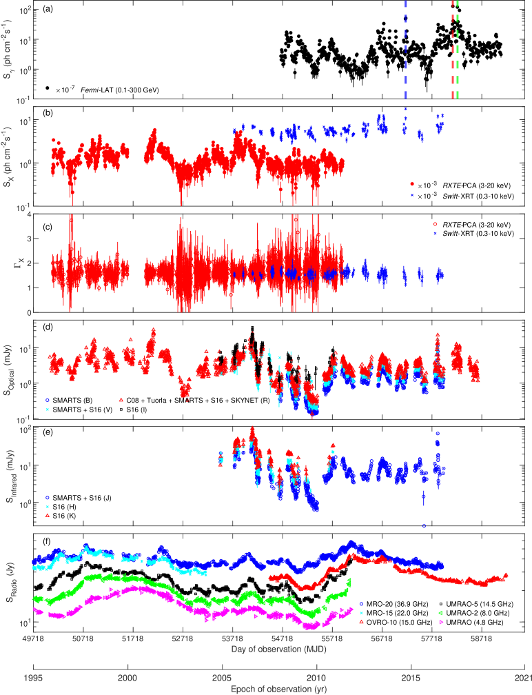
Figure 1: Multiwavelength light curves of the blazar 3C 279. Panel (a) gives the 7-day integration bin $\gamma$-ray fluxes from the Fermi-LAT satellite (0.1–300 GeV). The blue, red and green dashed vertical lines indicate three epochs for which 3-hr integration bin light curves are generated (panels a, b, and c of Figure 3). Panel (b) shows the X-ray fluxes from the RXTE-PCA (3–20 keV) and Swift-XRT (0.3–10 keV) satellites, respectively, while panel (c) gives the photon index derived by fitting a single power-law model to these datasets. Panels (d) and (e) give the $B$, $V$, $R$, $I$, $J$, $H$, and $K$-band fluxes from various, labeled, observing programs. Panel (f) gives radio fluxes, with noted offsets, from the Metsähovi (36.9 GHz and 22.0 GHz), OVRO (15 GHz) and UMRAO (14.5 GHz, 8.0 GHz, and 4.8 GHz) monitoring programs, respectively. Radio light curves for the entire duration of monitoring are given in Figure 4(a).

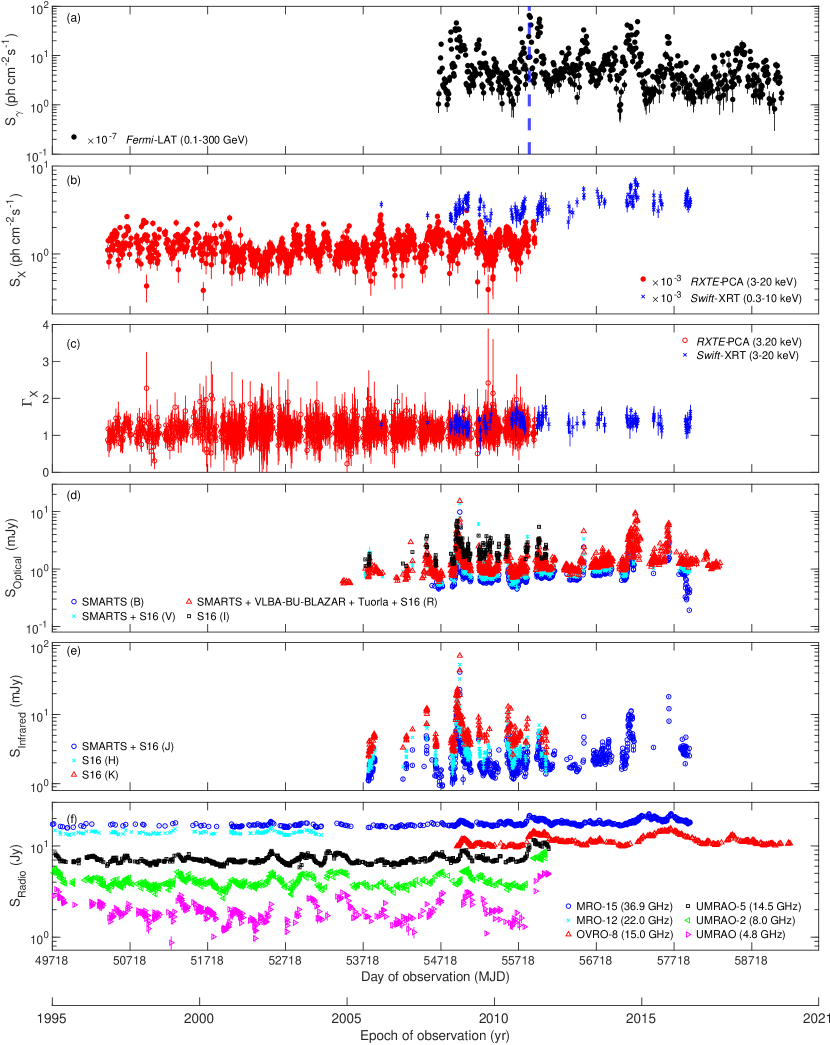
Figure 2: As in Figure 1, for the blazar PKS 1510$-$089. In panel (a) the blue dashed vertical line indicates an epoch for which 3-hr integration bin light curve is generated (panel (d) of Figure 3).

Table 1: Basic properties of the blazars 3C 279 and PKS 1510$-$089 studied here

Name	R.A.(J2000)	Dec.(J2000)	$z$	$M_{BH}$
	(h m s)	(∘ $\prime$ ${\prime\prime}$)		(108M⊙)
3C 279	12 56 11.166	$-$05 47 21.52	0.536a	3.0-8.0c
PKS 1510$-$089	15 12 50.532	$-$09 05 59.82	0.360b	0.4-0.7d

Note. — (1) the name of the blazar, (2-3) right ascension and declination from the NASA/IPAC Extragalactic Database (2019) (NED), (4) spectroscopic redshift. ^aMarziani et al. (1996); ^bThompson et al. (1990), (5) mass of the SMBH. ^c Hayashida et al. (2015); ^d Rakshit (2020).

The multiwavelength “snapshots” of blazar activity, i.e., the SEDs, can provide important clues to the emission processes and the physical parameters related to them within the relativistic jet, at least within a particular model set. This is usually attempted through solving the kinetic equation of the population of electrons injected with a certain energy distribution and evolving under radiative and adiabatic energy losses in, and escaping from, a single emission zone (Chiaberge & Ghisellini, 1999; Lindfors et al., 2005; Sikora et al., 2009; Abdo et al., 2011a, b; Paliya et al., 2015; Hayashida et al., 2015; Aleksić et al., 2015; Saito et al., 2015; Dutka et al., 2017; Hu et al., 2021). Such modeling efforts usually include an additional accretion disk component to fully describe the SED, although this component is more often necessary in the case of FSRQs (e.g., Castignani et al., 2013; Sbarrato et al., 2016) than for BL Lac objects (e.g., Kushwaha et al., 2018). Interestingly, the broad-band SEDs of the blazar PKS 1510$-$089 often reveal a prominent accretion disk component peaking at optical/$IR$ emission frequencies (Nalewajko et al., 2012) in contrast to the SEDs of the blazar 3C 279 which rarely show such a component (e.g., Hayashida et al., 2012, 2015, except during a low $\gamma$-ray activity state when an upturn at optical-UV wavelengths was attributed to an accretion disk component by Paliya et al. 2015). Studies of light curve variability and their PSDs provide information complementary to this as well as shedding some light on the jet dynamics and it is on this aspect that we focus in this paper. Finke & Becker (2014) analyzed the continuity equation in the Fourier-domain for the basic models mentioned above and predicted that PSD slopes at EC emission frequencies will be the same as that of the synchrotron emission frequencies (which is presumably more relevant for FSRQs). However, they found that the PSD slopes for the SSC emission frequencies varied with the slopes of the synchrotron emission frequencies (more relevant for BL Lac objects). Chen et al. (2016) included the effects of the decline of particle acceleration in this model setup and obtained PSDs at synchrotron and SSC emission frequencies. Breaks in PSDs on timescales of hours-days have been either identified with light-crossing, electron cooling, or escape timescales (Finke & Becker, 2014), or with relaxation timescales of the system (Chen et al., 2016).

Due to the availability of large datasets from various monitoring programs started some decades ago, although restricted to, at best, daily/weekly sampling of flux measurements, several groups have attempted to characterize the shape(s) of variability PSDs covering $\sim$3-3000 day timescales. In particular, using $\sim$30-40 years of radio data at 4.8, 8.0 and 14.5 GHz frequencies from the University of Michigan Radio Observatory (UMRAO) program, Park & Trippe (2017) reported $\beta$$\sim$1-3 for a sample of 43 blazars/AGNs. Max-Moerbeck et al. (2014) reported $\beta$$\sim$1.6-2.5 for a sample of 41 blazar sources using the 15 GHz radio light curves of 4-year duration from the Owens Valley Radio Observatory (OVRO) monitoring program. At optical frequencies, using the decade-long $R$-band data from the Tuorla Observatory monitoring program, Nilsson et al. (2018) reported $\beta$ $\sim$1-1.5 for a sample of 31 TeV detected blazars. At X-ray energies, using $\sim$2-3 day-long Advanced Satellite for Cosmology and Astrophysics (ASCA) and Rossi X-ray Timing Explorer (RXTE) datasets, Kataoka et al. (2001) reported $\beta$$\sim$1-1.5 for the blazars Mrk 421, Mrk 501 and PKS 2155$-$304 with a break in the PSD at a frequency of $\sim$10^-5 Hz (see also Isobe et al., 2015; Chatterjee et al., 2018, for confirmation of this break in the case of Mrk 421 using longer datasets). At high energy (HE) $\gamma$-ray energies using 11 months of the Fermi-Large Area Telescope (LAT) data, Abdo et al. (2010a) reported $\beta$$\sim$1-2 for a sample of 28 blazars; these slopes remain essentially unchanged when the PSD analyses were extended to longer timescales using the decade-long Fermi-LAT light curves (Meyer et al., 2019; Bhatta & Dhital, 2020; Tarnopolski et al., 2020). At VHE $\gamma$-ray energies, using $\geq$decade-long TeV light curves from the Very Energetic Radiation Imaging Telescope Array System (13.4 years) and High Energy Stereoscopic System (8.4 years) monitoring datasets, Goyal (2020) reported $\beta$$\sim$1 for the blazars Mrk 421 and PKS 2155$-$304, respectively.

Even though blazar emissions have been detected for over 18 decades of wavelengths and are variable over a wide range of timescales, very few efforts have been made to characterize the variability PSDs over different emission frequencies covering similar variability timescales for the same set of blazar sources; this is due to the lack of good quality datasets at a wide range of emission and variability frequencies. Notably, Chatterjee et al. (2008) performed the PSD analysis for the blazar 3C 279 at X-ray, optical, and radio frequencies using the decade-long RXTE-PCA data, $R$-band, and 14.5 GHz UMRAO datasets for the period 1996-2007. We revisit these results in the discussion. Chatterjee et al. (2012) reported similar PSDs slopes for a sample of 6 blazars using 2-year long $\gamma$-ray and optical/infrared light curves. Studies by Sandrinelli et al. (2016) and Sandrinelli et al. (2017) focussed on searching for quasi-periodic oscillations (QPOs) using $>$6-year long $\gamma$-ray and optical light curves of the blazar sources. Keeping this in mind, we started a program in 2015 to uniformly characterize the PSDs for many objects by uniquely selecting blazar sources for which long-duration ($>$decade), densely sampled (daily/weekly binned), high photometric accuracy ($\sim$1-15%) multiwavelength datasets exist for a large number of emission frequencies, either from public archives or from our own monitoring programs (particularly relevant for covering intranight timescales at optical frequencies). Our previous attempts focussed on characterizing the multiwavelength PSDs of the BL Lac objects PKS 0735+178 (radio, optical, and HE $\gamma$-ray energies; Goyal et al., 2017), OJ 287 (radio, X-ray, optical, HE $\gamma$-ray energies where the PSDs were characterized by modeling the light curves as a continuous-time auto regressive moving average process (CARMA); Goyal et al., 2018), Mrk 421 and PKS 2155$-$304 (radio, X-ray, optical, infrared, HE $\gamma$-ray, and VHE $\gamma$-ray energies; Goyal, 2020). Our main results were the following: (1) on timescales ranging from decades to months/days, the variability PSDs exhibited $\beta\sim$1 for X-rays, HE and VHE $\gamma$-rays and $\beta\sim$2 for the radio and optical/infrared frequencies; (2) the normalization of optical intranight PSDs turned out to be a smooth extrapolation from longer timescales; however, the PSD slopes showed a wider range with $\beta$$\sim$1-4, and; (3) more variability power was found on timescales $<$100 day in the X-ray and $\gamma$-ray bands as compared to lower energies. We discuss these results in Section 5.

In order to understand the underlying phyical processes responsible for the blazar emission and its variability, here we expand our efforts to study the shape of the multiwavelength variability PSDs of two bona-fide FSRQs, namely, 3C 279 ($z$=0.536) and PKS 1510$-$089 ($z$=0.360). Table 1 gives the basic properties of these sources. These FSRQs have been detected at VHE $\gamma$-ray energies (MAGIC Collaboration et al., 2008; H. E. S. S. Collaboration et al., 2013) and show rapid (minute-like) variability at Fermi-LAT energies (Foschini et al., 2011; Ackermann et al., 2016; Shukla & Mannheim, 2020). These FSRQs are well studied: 3C 279 (Hartman et al., 1992; Larionov et al., 2008a; Chatterjee et al., 2008; Abdo et al., 2010b; Hayashida et al., 2015); PKS 1510$-$089 (Abdo et al., 2010c; D’Ammando et al., 2011; Chen et al., 2012; Castignani et al., 2017; Ahnen et al., 2017). We selected these two sources as they have been a target of extensive multiwavelength campaigns including long-term monitoring with the RXTE-PCA instrument, thus allowing us to gather good-quality, long-duration light curves in the X-rays as well as at several GHz band radio frequencies, multiple infrared and optical bands, along with GeV $\gamma$-rays from the Fermi satellite. These light curves cover $\sim$6–30 yr durations with typical sampling intervals ranging from days to weeks depending on the monitoring program. The luminosity distances for 3C 279 and PKS 1510$-$089 are 3.1 Gpc and 1.9 Gpc, respectively, computed using the cosmological calculator (Wright, 2006) and assuming a concordant cosmology with the Hubble constant $H_{0}=$ 69.6 km s^-1 Mpc^-1, $\Omega_{\rm m}=$ 0.286, and $\Omega_{\Lambda}=$ 0.714 (Bennett et al., 2014).

This paper is organized as follows. Section 2 gives details on the data acquisition and the generation of multiwavelength light curves. Section 3 describes the analysis methods, in particular, the derivation of PSDs and the estimation of the best-fit PSD shape using numerical simulations of the light curves. Section 4 provides the main results while the discussion and summary are given in Section 5.

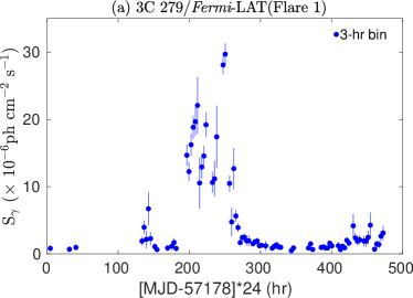
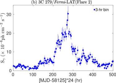
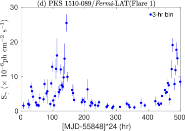
Figure 3: Fermi-LAT light curves obtained using 3-hr integration binning interval for selected time ranges for 3C 279 (panels a, b, and c) and PKS 1510$-$089 (panel d).

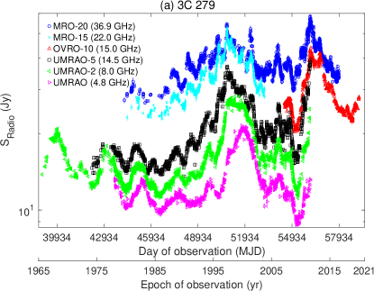
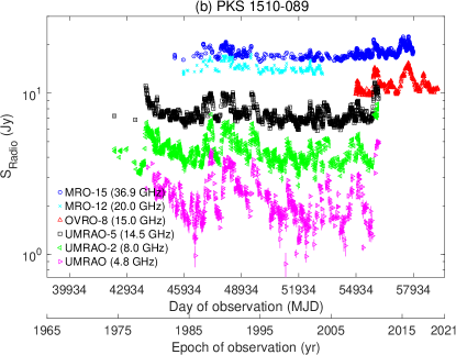
Figure 4: Multifrequency radio light curves for the entire duration of monitoring for the FSRQs 3C 279 (a) and PKS 1510$-$089 (b). The GHz band radio fluxes, with noted offsets, are from the Metsähovi (36.9 GHz and 22.0 GHz), OVRO (15 GHz), and UMRAO (14.5 GHz, 8.0 GHz, and 4.8 GHz) monitoring programs, respectively.

2 Multiwavelength light curves

2.1 HE  $\gamma$-rays: Fermi-LAT

We analyzed the Fermi-LAT (Atwood et al., 2009, 2013; Bruel et al., 2018) data for 3C 279 and PKS 1510$-$089 for the 0.1–300 GeV band, for the period 2008 August 8 – 2020 September 16 with an integration time of seven days using the Fermi ScienceTools package Fermitools-conda (version 2.0.18) available from Fermi Science Support Center (FSSC) and the latest instrument response function p8r3_source_v3. The standard unbinned likelihood analysis was performed. The procedure started with selecting the events for a time interval (1-week) with standard quality cuts (DATA_QUAL$>$0)&&(LAT_CONFIG == 1) and zenith angle cut of $\theta$ $<$ 90^∘ to avoid contamination from the Earth’s limb using the tasks gtselect and gtmktime. For the target, we selected a 20^∘$\times$20^∘ region of interest (ROI) centered at the source catalog position. Next, the exposure map was created from the livetime cube (gtltcube) using the task gtexpmap with a total of 35 logarithmically spaced energy intervals bounded within 0.1-300 GeV. The choice of energy resolution is governed by the FSSC recommendation, as 10 bins per decade was found to be sufficient to accommodate the change in effective area below $\sim$1 GeV. Finally, in the likelihood analysis (gtlike), all the sources from data release 2 (DR2) of the 10-yr Fermi-LAT catalog (4FGL-DR2; Abdollahi et al. 2020; Ballet et al. 2020), within a 30^∘ radius of the target were included, as were the standard templates for diffuse emission from our Galaxy (gll_iem_v07.fits) and the isotropic $\gamma$-ray background (iso_p8r3_source_V3_v1.txt). In the fitting (gtlike), the spectral normalization of the target and sources within 5^∘ of the ROI center were allowed to be free while for the remaining sources the spectral shapes were fixed at their catalog-derived values. The normalization of the Galactic diffuse background was kept frozen while that of the isotropic $\gamma$-ray background component was allowed to vary. Specifically, the $\gamma$-ray spectra of the targets were modeled with a log-parabolic function given by the 4FGL-DR2 catalog. The light curves were generated including 0.1-300 GeV fluxes for which the test statistic (TS; defined as twice the difference between the log-likelihood which is maximized by adjusting all the parameters of the model computed with and without including the source; Mattox et al. 1996) was found to be $>$10. This gives us preliminary light curves for 3C 279 and PKS 1510$-$089.

Next, we checked for the contamination of the targets’ fluxes due to proximity to, or occultation by, the Sun and the Moon as it has been demonstrated that the Sun and the Moon are sources of $\gamma$-ray emission (Abdo et al., 2011c, 2012). We extracted the equatorial positions (R.A. and Dec.) of the Sun at mission elapsed time (MET) from the spacecraft files and computed the angular distances from the targets in the sky plane. The Sun is known to occult 3C 279 on October 8 each year (Barbiellini et al., 2014). The closest distance between the Sun and PKS 1510$-$089 is $\approx$8.5^∘, occurring on November 11. Similarly, the positions (R.A. and Dec.) of the Moon were computed at the METs given in the spacecraft files in the Geocentric Celestial Reference System (GCRS) using the get_moon task from the astropy.coordinates library and the angular distances between the targets and Moon were computed. The Moon occults 3C 279 while the closest distance between the Moon and PKS 1510$-$089 is $\sim$3.2^∘. For the blazar 3C 279, we extracted all the weekly time bins for which the distances between the targets and the Sun/Moon were found to be smaller than 10^∘ and analyzed them separately. As the Moon moves much faster than the Sun in the sky plane ($\sim$13^∘ day^-1 and $\sim$1^∘ day^-1, respectively) and therefore, is expected to occult 3C 279 more often than the Sun, we proceeded to account for the contamination due to Sun/Moon to the target fluxes in two steps.

First, we extracted all the weekly time bins for which the angular distances between the Moon and 3C 279 were found to be $<$10^∘ without having the Sun nearby (i.e., the angular distance between the Sun and 3C 279 was $>$20^∘). Of these, we randomly selected a few time bins during which the Moon was passing the target’s ROI (separation $<$10^∘). We generated the lunar templates for these bins following the FSSC guidance. The description of the Solar System Tools which models the quiescent emission from the Sun and Moon is given in Johannesson & Orlando (2013). An all-sky livetime cube was generated for the lunar emission using the task gtltcube2 with 35 logarithmically spaced energy intervals with livetime cube and counts map option from the output of the task gtbin. Next, we generated the livetime cube for the Moon using the task gtltcubesun with body=Moon and instrument angle=1^∘. As a final step, the template for the Moon emission was generated using the task gtsuntemp using the lunar profile template and the all-sky livetime cube generated from the task gtltcube2. Finally, the Moon template was included in the model file for the likelihood analysis. The Moon’s SED was modeled as a power-law for which the normalization was allowed to vary while the index was fixed during the fitting. We compared the target fluxes with and without including the Moon template in the likelihood analysis and found that the change in flux (before Moon - after Moon/before Moon) was comparable to the measurement uncertainties in the weekly time bins with TS$>$10. Thus, we conclude that the Moon does not have a significant impact on the weekly binned fluxes of 3C 279.

Next, we proceeded to compute the contamination due to the Sun’s proximity to 3C 279. We generated the solar template following the same steps needed to generate the lunar template with appropriate changes in input parameters (such as including body=Sun and instrument angle=180^∘ in the task gtltcubesun) and the likelihood analysis was performed. The normalization of the power-law SED of the Sun was allowed to vary while the index was fixed during the fitting. We compared the change in flux (before Sun-after Sun/before Sun) and found that for a few time bins, the change in target flux was up to 50% of the non-corrected value when the solar template was included in the model fitting. In two time bins, 3C 279 was detected with TS$<$10 (as compared to TS$>$10 without including the solar template). In general though we found that the change in flux is lower ($<$10%) and therefore comparable to measurement uncertainties when the Sun was $>$2^∘ away from the target. In a few time bins analyzed, the target and the Sun’s fluxes were found to be highly correlated (correlation coefficient $>$0.5), so the flux measurements in these time bins were discarded. The final light curve of the blazar 3C 279 (Figure 1) includes all flux measurements corrected for solar emission and TS$>$10.

Since the analysis performed for weekly integrated time bins for 3C 279 indicated negligible change when the Sun is $>$2^∘ away from the target, we did not perform the checks for the Sun’s contamination for PKS 1510$-$089 (closest distance$>$8^∘). We also did not correct for the Moon’s contamination as weekly integrated fluxes did not show a significant change in flux after the inclusion of the lunar template. Figure 2 shows the final light curve including measurements with TS$>$10.

In order to extend the gamma-ray PSD temporal range down to hourly timescales we needed to examine periods of high-fluxes. So we generated short-duration (3-weeks) LAT light curves using a 3-hr integration binning interval for time ranges when the daily LAT flux from the sources exceeded 1$\times$10^-5 ph cm^-2 s^-1. We selected three time ranges for the blazar 3C 279, denoted as ‘Flare 1’ (Cutini, 2015; Ackermann et al., 2016), ‘Flare 2’ (van Zyl & Ojha, 2018), and ‘Flare 3’ (Ojha & van Zyl, 2018), respectively. For the blazar PKS 1510$-$089, we selected one time range, denoted as ‘Flare 1’ (Hungwe et al., 2011; Orienti et al., 2013). In each case, the selected time range was centered around the day of the flare. The analysis was performed in a similar fashion as that of 1-week integration time bins. The final light curves were checked for the goodness of gtlike results by plotting Flux/$\Delta$Flux vs. $\sqrt{TS}$. For a good fit, one expects a linear trend between these quantities. We removed one flux point from the ‘Flare 3’ and ‘Flare 1’ light curves of 3C 279 and PKS 1510$-$089, respectively, which did not follow a linear trend. For 3C 279, we checked for the contamination due to the Moon alone as the selected time ranges did not coincide with the passage of the Sun. We note that the change in flux due to inclusion of lunar templates was $<$30%, i.e., within the measurement uncertainties provided by these measurements. Therefore, we conclude that the occultation of the Moon does not have a significant effect on 3-hr integration bin flux measurements. For PKS 1510$-$089, the selected time range did not coincide with the passage of the Moon in the ROI ($>$10^∘). Therefore, we do not correct for the Moon’s effect in the 3-hr integration bin light curves for either of the targets. Figure 3 gives the 3-hr integration bin light curves for ‘Flare 1’, ‘Flare 2’, and ‘Flare 3’ for the blazar 3C 279 (panels a, b, and c) and ‘Flare 1’ for the blazar PKS 1510$-$089 (panel d).

2.2 X-rays: RXTE-PCA and Swift-XRT

We downloaded the 1998 and 1334 Stdprods (Standard2 data product) for 3C 279 and PKS 1510$-$089, respectively, from the RXTE quick look analysis from the HEASARC website. These source and background Standard2 spectra were reduced by a pipeline using a standard set of FTOOLS and PCA backgrounds with a general script and employed one single set of filtering criteria for all observations. The Standard2 mode of PCA has 129 energy channels, covering the entire range 2–25 keV of the PCA detector. The spectra were fitted within the energy range 3.0–20.0 keV with a power-law of the form $F(E)=F_{0}E^{-\Gamma_{X}}$, where $F_{0}$ is the normalization and $\Gamma_{X}$ is the photon index, found via xspec with $\chi^{2}$ statistics. In the spectral analyses, the Galactic absorption corresponding to neutral hydrogen column density in the direction of the source was fixed (Kalberla et al., 2005). The unabsorbed photon fluxes were obtained within the 3–20 keV energy range by fitting wabs*cpflux*powerlaw. We averaged the fluxes using a binning interval of 1 day. Figures 1(b) and  2(b) show these X-ray photon fluxes for 3C 279 and PKS 1510$-$089, respectively. A few earlier studies report part of the RXTE-PCA datasets examined by us for 3C 279 (Hartman et al., 2001; Larionov et al., 2008b; Böttcher et al., 2007; Chatterjee et al., 2008; Abdo et al., 2010b) and PKS 1510$-$089 (Marscher et al., 2010; Castignani et al., 2017).

The archival data from the Swift-XRT (Gehrels et al., 2004), consisting of 415 and 262 pointed observations made between 2005 September 17 and 2016 July 17, for the blazars 3C 279 and PKS 1510$-$089, respectively, were also analyzed by us. We used the latest version of the calibration database (CALDB) and version 6.19 of the heasoft package. For each dataset, we used the level 2 cleaned event files of the ‘photon counting’ (PC) and ‘window timing’ (WT) data acquisition modes generated using the standard xrtpipeline tool. The details of the XRT data analysis are given in Goyal et al. (2018) and Goyal (2020) and we briefly outline the procedure here. For the PC mode data, the source and background spectra were generated using a circular aperture with appropriate region sizes and grade filtering using the xselect tool. An aperture radius of $47^{\prime\prime}$ around the source position and four source-free regions of $118^{\prime\prime}$ radius were used to estimate the source and background spectra, respectively. For the WT mode data, the source region of $47^{\prime\prime}$ circular aperture and an annular region with inner and outer radii of $187^{\prime\prime}$ and $281^{\prime\prime}$, respectively, for background estimation were selected to estimate the source and background spectra. Following the XRT tutorial, appropriate corrections were made in the ‘BACKSCAL’ keyword in the extracted source and background spectra to account for the different sizes of the source and background estimation regions. We also checked for the recommended pile-up limit for the PC ($\sim$0.5 count s^-1) and WT ($\sim$100 count s^-1) modes. The ancillary response matrix was generated using the task xrtmkarf for the exposure map generated by xrtexpomap. All the source spectra were then binned over 20 points and corrected for the background using the task grppha. For each exposure, the spectral analysis between 0.3 and 10 keV was performed in an identical manner to that of the RXTE-PCA data. The unabsorbed 0.3–10 keV photon fluxes were averaged using a 1-day binning interval and these light curves are shown in Figures 1(c) and Figure 2(c) for the targets 3C 279 and PKS 1510$-$089, respectively. In addition, we show the fitted ${\Gamma_{X}}$ for the RXTE-PCA and Swift-XRT datasets analyzed in Figures 1(c) and  2(c) for the targets 3C 279 and PKS 1510$-$089, respectively. A few earlier studies report part of the Swift-XRT datasets analyzed by us for 3C 279 (Abdo et al., 2010b; Hayashida et al., 2015; Larionov et al., 2020) and PKS 1510$-$089 (Abdo et al., 2010c; D’Ammando et al., 2011; Nalewajko et al., 2012).

Table 2: Summary of the observation and PSD analysis

Light Curve (Energy Range)	Epoch of Monitoring	$N_{obs}$	$T_{\rm total}$	$T_{\rm mean}$	$T_{\rm in}$	Varsp	$\rm\log_{10}(P_{\rm stat})$	$\log_{10}(\nu_{k})$ Range	$\beta\pm$err	$p_{\beta}^{b}$
	(Start-End)		(yr)	(day)	(day)		($\frac{\mathrm{r}ms}{\mathrm{m}ean})^{2}$day	(day-1)
3C 279
Fermi-LAT (0.1–300 GeV)	2008 Aug 8 - 2020 Sep 16	601	12.1	7.3	1.0	0.25	$-$0.84	$-$3.64 to $-$1.40	1.0$\pm$0.7	0.595
RXTE-PCA (3–20 keV)	1996 Jan 22 - 2011 Dec 30	1751	15.9	3.3	0.5	3.16	$-$0.96	$-$3.76 to $-$1.11	1.2$\pm$0.3	0.496
Swift-XRT (0.3–10 keV)	2006 Jan 13 - 2017 Jun 28	230	11.5	18.2	0.5	2.57	$-$0.43	$-$3.62 to $-$1.78	1.4$\pm$0.7	0.999
Optical (B)	2008 May 17 - 2017 Jul 19	624	9.2	5.4	0.5	3.05	$-$1.41	$-$3.52 to $-$1.28	1.8$\pm$1.3	0.567
Optical (V)	2005 Apr 7 - 2017 Jul 19	775	12.3	5.8	0.5	3.26	$-$0.21	$-$3.65 to $-$1.20	2.1$\pm$1.4	0.651
Optical (R)	1995 Nov 25 - 2019 Jun 4	1829	23.5	4.7	0.5	3.17	$-$1.24	$-$3.93 to $-$1.07	1.4$\pm$0.5	0.635
Optical (I)	2005 Apr 2 - 2011 Jan 30	183	6.2	12.5	0.5	2.82	$-$0.15	$-$3.35 to $-$1.53	1.6$\pm$1.8	0.924
Infrared (J)	2005 Apr 9 - 2017 Jul 18	727	12.3	6.2	0.5	3.34	$-$1.37	$-$3.65 to $-$1.20	2.1$\pm$1.5	0.832
Infrared (H)	2005 Apr 9 - 2011 Jun 23	197	6.2	11.5	0.5	3.37	$-$0.83	$-$3.35 to $-$1.53	1.8$\pm$1.8	0.994
Infrared (K)	2005 Apr 9 - 2011 Jun 23	170	6.2	13.3	0.5	3.58	$-$0.31	$-$3.35 to $-$1.53	2.9$\pm$1.6	0.992
MRO (36.9 GHz)	1979 Dec 21 - 2017 Jun 19	1740	37.5	7.9	0.5	2.97	$-$1.68	$-$4.13 to $-$1.48	1.7$\pm$0.3	0.968
MRO (22.0 GHz)	1980 Jun 19 - 2004 Jun 21	751	24.0	11.7	0.5	2.55	$-$1.38	$-$3.94 to $-$1.49	2.9$\pm$1.1	0.225
OVRO (15 GHz)	2008 Jan 8 - 2020 Dec 26	535	13.0	8.9	0.5	1.35	$-$2.11	$-$3.67 to $-$1.43	2.5$\pm$1.1	0.813
UMRAO (14.5 GHz)	1974 May 8 - 2012 Jun 23	1567	38.1	8.9	0.5	2.00	$-$2.39	$-$4.14 to $-$1.49	2.6$\pm$1.0	0.977
UMRAO (8.0 GHz)	1965 Aug 13 - 2012 May 16	1653	46.8	10.3	0.5	1.59	$-$2.40	$-$4.23 to $-$1.52	2.4$\pm$0.9	0.871
UMRAO (4.8 GHz)	1978 Apr 15 - 2012 Jun 14	1101	34.2	11.3	0.5	1.64	$-$2.46	$-$4.09 to $-$1.64	2.1$\pm$0.6	0.309
Flare 1a (0.1–300 GeV)	2015 Jun 5 - 2015 Jun 26	80	0.057	0.24	0.042	1.84	$-$1.45	$-$1.29 to $+$0.11	1.4$\pm$3.9	0.500
Flare 2a (0.1–300 GeV)	2018 Jan 7 - 2018 Jan 28	146	0.057	0.14	0.042	0.38	$-$1.88	$-$1.31 to $+$0.30	2.0$\pm$2.8	0.808
Flare 3a (0.1–300 GeV)	2018 Apr 13 - 2018 May 4	157	0.057	0.14	0.042	0.27	$-$2.35	$-$1.31 to $+$0.30	1.5$\pm$2.9	0.680
PKS 1510$-$089
Fermi-LAT (0.1–300 GeV)	2008 Aug 8 - 2020 Sep 16	603	12.1	7.3	1.0	0.30	$-$0.76	$-$3.64 to $-$1.40	0.9$\pm$0.6	0.300
RXTE-PCA (3–20 keV)	1996 Dec 13 - 2011 Dec 30	1252	15.1	4.4	0.5	1.47	$-$0.79	$-$3.73 to $-$1.08	1.4$\pm$0.3	0.482
Swift-XRT (0.3–10 keV)	2006 Aug 4 - 2017 Jun 26	181	10.9	22.0	0.5	3.04	$-$0.25	$-$3.59 to $-$1.76	1.5$\pm$1.0	0.994
Optical (B)	2008 May 17 - 2017 Jun 14	542	9.1	6.1	0.5	3.29	$-$2.26	$-$3.52 to $-$1.28	1.5$\pm$0.5	0.185
Optical (V)	2006 Jan 10 - 2017 Jun 14	611	11.4	6.8	0.5	3.48	$-$1.27	$-$3.62 to $-$1.38	1.2$\pm$0.3	0.003
Optical (R)	2005 Mar 25 - 2018 Jul 10	1207	13.3	4.0	0.5	3.12	$-$2.15	$-$3.68 to $-$1.03	0.7$\pm$0.4	0.532
Optical (I)	2006 Jan 11 - 2012 May 28	225	6.4	10.3	0.5	3.75	$-$1.09	$-$3.36 to $-$1.12	0.7$\pm$0.8	0.245
Infrared (J)	2006 Feb 17 - 2017 Jun 11	675	11.3	6.1	0.5	3.86	$-$1.75	$-$3.61 to $-$1.37	0.2$\pm$1.9	0.317
Infrared (H)	2006 Feb 17 - 2012 Jun 1	304	6.3	7.5	0.5	4.06	$-$1.44	$-$3.36 to $-$1.32	1.3$\pm$4.4	0.003
Infrared (K)	2006 Feb 22 - 2012 Jun 1	223	6.3	10.3	0.5	3.59	$-$1.27	$-$3.36 to $-$1.52	0.2$\pm$2.1	0.011
MRO (36.9 GHz)	1983 Apr 16 - 2017 Jun 19	885	34.2	14.1	0.5	2.51	$-$0.97	$-$4.09 to $-$1.65	1.8$\pm$0.7	0.559
MRO (22.0 GHz)	1984 Jul 12 - 2004 Jun 21	239	19.9	30.5	0.5	1.44	$-$0.52	$-$3.86 to $-$2.03	1.4$\pm$0.5	0.386
OVRO (15.0 GHz)	2009 Apr 2 - 2020 Dec 27	427	11.7	10.0	1.0	1.18	$-$2.17	$-$3.63 to $-$1.39	2.1$\pm$1.0	0.505
UMRAO (14.5 GHz)	1974 Aug 14 - 2012 Jun 27	1345	37.9	10.3	0.5	3.41	$-$1.70	$-$4.14 to $-$1.48	1.6$\pm$0.4	0.145
UMRAO (8.0 GHz)	1974 Sep 4 - 2012 May 18	1147	37.7	12.0	0.5	1.68	$-$1.55	$-$4.13 to $-$1.48	1.6$\pm$0.3	0.164
UMRAO (4.8 GHz)	1979 Mar 23 - 2012 Jun 16	672	33.2	18.1	0.5	1.56	$-$1.19	$-$4.08 to $-$1.64	1.7$\pm$0.3	0.199
Flare 1a (0.1–300 GeV)	2011 Oct 14 - 2011 Nov 4	74	0.057	0.27	0.042	0.95	$-$1.34	$-$1.31 to $+$0.09	1.5$\pm$3.6	0.978

Note. — (1) the instrument/band (energy range/frequency band used for observations in parentheses); ^a refers to Fermi-LAT light curves made with 3-hr integration bins (Figure 3), (2) the beginning and ending dates of the light curve used, (3) the number of data points in the light curve, (4) the total duration of the observed light curve, (5) the mean sampling interval of the light curve (= Col. 4/Col. 3), (6) the interpolation interval used in the PSD analysis, (7) square root of the variance of the sampling pattern for the data normalized by $T_{\rm mean}$, (8) the noise level in the PSD due to the measurement uncertainty, (9) the temporal frequency range covered by the binned logarithmic power spectrum, (10) the best-fit power-law slope of the PSD derived using the PSRESP method along with the corresponding errors representing the 98% confidence limit (see Section 3.2) (11) the corresponding $p_{\beta}$: ^b a power-law model is considered a poor fit for $p_{\beta}\,<\,0.1$ as the corresponding rejection confidence for the model is $\geq$90% (Section 3.2).

2.3 Optical and Infrared: SMARTS, REM, Tuorla, VLBA-BU-BLAZAR, and SKYNET monitoring

The blazars 3C 279 and PKS 1510$-$089 have been the targets of regular monitoring on daily timescales at multiple optical ($B$, $V$, $R$, and $I$) and Infrared ($J$, $H$, and $K$) bands and here we combine many of these observations. We begin by using publicly available $B$, $V$, $R$, $J$, and $K$-band light curves from the Small and Moderate Aperture Research Telescope System (SMARTS; Bonning et al. 2012) program coordinated by Yale University for the period $\sim$2008 until 2017. We also take $V$, $R$, $I$, $J$, $H$, and $K$-band light curves, covering the period 2005–2012, from the Rapid Eye Mounting telescope (REM; Zerbi et al. 2001) which were published in Sandrinelli et al. (2016, S16 hereafter). Many $R$-band optical photometric data were also obtained from the Tuorla Blazar monitoring program for the period 2004–2016 (Takalo et al., 2008) and those published in Chatterjee et al. (2008, C08 hereafter) for the period 1996-2004. Additionally, for the blazar PKS 1510$-$089 $R$-band photometric data were obtained from the VLBA-BU-BLAZAR blazar monitoring program for the period 2005–2018 (Jorstad & Marscher, 2016). For the blazar 3C 279, additional $R$-band photometric data for the period 2018–2019 were obtained from the Skynet Robotic Telescope Network program (SKYNET).

There is a great deal of overlap between the SMARTS and the REM programs’ data in the $V$, $R$, $J$, and $K$-bands and they complement each other well at $V$, $R$, and $J$-bands, with the pairs of magnitudes within 0.1 mag on the same nights, consistent with the calibration uncertainties provided by these programs. Moreover, the $R$-band photometric data obtained from the VLBA-BU and the Tuorla monitoring programs are comparable to other datasets within the measurement uncertainties ($<$0.1 mag) on the same nights. As a majority of these programs have mean sampling intervals $>$1-day, we have combined the datasets at $V$, $R$, and $J$-bands and average magnitudes were computed with 1-day binning intervals. This is done to avoid obtaining poor sampling on intranight timescales as well as to obtain homogeneous sampling on daily timescales. On the other hand, the $K$-band magnitudes from the SMARTS program has a magnitude offset $\geq$0.1 mag from that provided by S16 on the same nights. On visual inspection, the $K$-band SMARTS light curve appears more variable than the S16 light curve on similar timescales. Therefore, in this study, we use only the $K$-band data provided by S16. On a few occasions, fluxes at $B$, $I$, $H$, and $K$-bands were also obtained multiple times on a given night and we have averaged those observations over a 1-day binning interval.

Next, the optical and infrared magnitudes, $m$, were converted to flux densities using $m_{zero}$ $\times 10^{-0.4\times\,m}$, where $m_{zero}$ (=4063 Jy, 3636 Jy, 3064 Jy, 2635 Jy, 1590 Jy, 1020 Jy, and 600 Jy for the $B$, $V$, $R$, $I$, $J$, $H$, and $K$-bands, respectively) refer to zero-point magnitude fluxes of the photometric system (Glass, 1999). The errors in fluxes were derived using standard error propagation (Bevington & Robinson, 2003). The resulting optical and infrared-band light curves for the targets 3C 279 and PKS 1510$-$089 are presented in Figures 1(d, e) and  2(d, e), respectively.

2.4 Radio: MRO, UMRAO, and OVRO

GHz-band radio light curves of the targets were gathered from the Aalto University Metsähovi Radio Observatory (MRO) at 36.9 and 22.0 GHz (Teraesranta et al., 1998), the UMRAO at 14.5, 8.0, and 4.8 GHz (Aller et al., 1999), and the OVRO monitoring programs at 15 GHz (Richards et al., 2011). All the light curves gathered were binned using 1-day binning intervals as the typical sampling intervals of these programs are much larger ($>$3 days to 2 weeks). The radio light curves of the blazars 3C 279 and PKS 1510$-$089 for periods (1995–2017) that overlap monitoring with other frequencies are presented in Figures 1(f) and  2(f), respectively. The radio light curves for the full durations of the monitoring are shown in panels (a) and (b) of Figure 4.

3 PSD Analysis

The derivation of PSDs using the discrete Fourier transformation (DFT) and the estimation of spectral shapes using the ‘power spectral response (PSRESP)’ method are given in detail in Goyal (2020, 2021). Here we provide the main features.

3.1 Derivation of PSDs: discrete Fourier transform

The rms-normalized periodogram is given as the squared modulus of its DFT for the evenly sampled light curve $f(t_{i})$, observed at discrete times $t_{i}$ and consisting of $N$ data points,

$$P(\nu_{k}) =  \frac{2\,T}{\mu^{2}\,N^{2}}\,\Bigg{\{}\Bigg{[}\sum_{i=1}^{N}f(t_{i})\,\cos(2\pi\nu_{k}t_{i}) \Bigg{]}^{2} +\\ \Bigg{[}\sum_{i=1}^{N}f(t_{i})\,\sin(2\pi\nu_{k}t_{i}) \Bigg{]}^{2}\,\Bigg{\}},$$ (1)

where $\mu$ is the mean of the light curve and is subtracted from the flux values, $f(t_{i})$. The DFT is computed for evenly spaced frequencies ranging from the total duration of the light curve, $T$, down to the Nyquist sampling frequency ($\nu_{\rm Nyq}$). Specifically, in our analysis, the frequencies corresponding to $\nu_{k}=k/T$ with $k=1,...,N/2$, $\nu_{\rm Nyq}=N/2T$, and $T=t_{N}-t_{1}$ are considered. The constant noise floor level from measurement uncertainties is computed using (Isobe et al., 2015):

$$P_{\rm stat}=\frac{2\,T}{\mu^{2}\,N}\,\sigma_{\rm stat}^{2}\,,$$ (2)

where, $\sigma_{stat}^{2}=\sum_{j=1}^{j=N}\Delta f(t_{j})^{2}/N$ is the mean variance of the measurement uncertainties for the flux values, $\Delta f\!(t_{j})$, in the observed light curve at times $t_{j}$, with $N$ denoting the number of data points in the observed light curve. As expected, the noise floor level due to measurement uncertainties has a white noise character as the variability power contributed by measurement uncertainties alone is equal at all variability frequencies.

The unevenly sampled time series is rendered evenly sampled through linear interpolation between two consecutive data points with the interpolation interval, $T_{in}$, roughly 5–10 times smaller than the mean observed sampling interval; otherwise, the ‘spectral window function’ corresponding to the sampling times gives a non-zero response in the Fourier domain, resulting in spurious powers in the periodograms (see, Appendix A of Goyal, 2020). In this work, the PSDs have been generated for the actual duration of the light curves down to the mean (observed) sampling intervals, $T_{\rm mean}$. We note that interpolation is a smoothing operation, so it alters the high-frequency PSD of a data set, and this would be very obvious if we reported the spectrum up to 1/(2*$T_{in}$). The effects are reduced by cutting it off at 1/(2*$T_{\rm mean}$), but it does not necessarily solve the problem. It depends on how much the actual sampling varies, or equivalently what the typical distance between the actual data point and the interpolate point used in the spectrum at  1/(2*$T_{\rm mean}$) is. Since the light curves are relatively densely sampled, the PSDs have adequate coverage of many different frequencies. We expect a little extra noise because we do not have as many data pairs per frequency as would be the case for even sampling. These ramifications are not problematic in our case as we have plenty of coverage of the frequencies, and gridding the data is simply expedient. We demonstrate this qualitatively by calculating the typical separation of each sampling point from the even (i.e., $T_{\rm mean}$) grid and computing the variance of it. For our light curves, we computed the square root of the variance of the sampling pattern normalized by $T_{\rm mean}$, Var_sp= variance^1/2/$T_{\rm mean}$ (Column 7 of Table 2). This value should be zero for precisely evenly sampled data. As can be seen from Table 2, these values are close to zero for weekly-binned and $<$2 for 3-hr binned Fermi-LAT light curves for both targets, as they are better sampled. For the optical and infrared light curves, the values range between $\sim$3.0 and $\sim$4.0 because of the relatively large (4–6 months) systematic gaps in monitoring due to the target’s proximity to the Sun. For the X-ray and GHz band radio light curves, these values range between $\sim$1.4 and $\sim$3.0 for the majority of the gathered light curves, except for the 14.5 GHz UMRAO light curve for the target PKS 1510$-$089 for which it is 3.4. As only relatively small (weeks) systematic gaps are expected in the RXTE, Swift, and the radio data because of pointing constraints due to the target’s proximity to the Sun, these light curves can be considered better sampled than the optical ones. Since for the great majority of our data, these Var_sp values are relatively small numbers, our cutting the spectrum down to 1/(2*$T_{\rm mean}$) does not alter its shape.

The sampling distribution and the corresponding spectral window functions of the observed light curves are shown in Appendices A.1 and  A.2 for the blazars 3C 279 and PKS 1510$-$089, respectively. In our analysis, to avoid the distortions introduced due to the finite duration of the light curve, known as ‘red-noise leakage’, the PSDs are generated using the ‘Hanning’ window function (e.g., Press et al., 1992; Max-Moerbeck et al., 2014). The distortions in the PSD due to discrete sampling of the time series, i.e., aliasing, are not serious for red-noise dominated time series and usually contribute a small amount of power at all frequencies (Uttley et al., 2002). The ‘raw’ periodograms, obtained using Eq. (1), provide a noisy estimate of the spectral power (as it consists of independently distributed $\chi^{2}$ variables with two degrees of freedom (DOF); Timmer & Koenig, 1995; Papadakis & Lawrence, 1993; Vaughan et al., 2003); therefore, we average a number of them to obtain a reliable estimate. A binning factor of 1.6 is used, with the representative frequency taken as the geometric mean of each bin in our analysis (except for R-band and 8.0 GHz PSDs of 3C 279 for which a binning factor of 1.4 is used). Next, the ‘true’ power spectrum in the log-log space is obtained by offsetting the observed power spectrum by the expectation value of a $\chi^{2}$ distribution with 2 DOF, which is equal to $-$0.25068 (Vaughan, 2005).

Table 3: Mean PSD slope estimates

Frequency band	$\beta_{\rm mean}\pm$err	Frequencies used for averaginga
3C 279
radio-synchrotron	2.34$\pm$0.16	MRO (36.9 and 22.0 GHz), UMRAO (14.5, 8.0, and 4.8 GHz)
optical-synchrotron	1.95$\pm$0.22	$B$, $V$, $R$, $I$, $J$, $H$, and $K$
IC	1.20$\pm$0.15	RXTE, Swift, and Fermi-LAT
PKS 1510$-$089
radio-synchrotron	1.60$\pm$0.08	MRO (36.9 and 22.0 GHz), UMRAO (14.5, 8.0, and 4.8 GHz)
optical-synchrotron	0.77$\pm$0.23	$B$, $R$, $I$, and $J$
IC	1.30$\pm$0.16	RXTE, Swift, and Fermi-LAT

Note. — (1) name of the frequency band, (2) mean PSD slope and the corresponding 1$\sigma$ error, (3) frequencies used for averaging to obtain the mean PSD slope; ^aOnly PSD slopes with $p_{\beta}>$0.1 are used to estimate the $\beta_{\rm mean}$ in the representative frequency band (see Table 2).

3.2 Estimation of the spectral shape: the PSRESP method

As the PSDs are subjected to various distortions due to Fourier transformation, the PSRESP method is an efficient approach to obtain a best-fit spectral model (e.g., Uttley et al., 2002; Chatterjee et al., 2008; Max-Moerbeck et al., 2014; Meyer et al., 2019). We have previously employed this method in Goyal (2020) and Goyal (2021); therefore, we only briefly discuss its main features here. In this method, an (input) PSD model is tested against the observed PSD and the estimation of best-fit model parameters and their uncertainties is performed by varying the model parameters. A large number of mock light curves are generated with a known underlying power-spectral shape via Monte Carlo (MC) simulations. These simulated light curves are rebinned to mimic the observed data and subjected to the Fourier transformation in exactly the same manner as that of the observed data. The averaging of a large number of such PSDs gives the mean of the distorted model (input) power spectrum while the standard deviation around the mean periodogram gives the errors on the modeled (input) power spectrum. The goodness of fit of the model is estimated by computing two functions, similar to $\chi^{2}$, defined as

$$\chi^{2}_{\rm obs}=\sum_{\nu_{k}=\nu_{min}}^{\nu_{k}=\nu_{max}}\frac{[\overline{\log_{10}P_{\rm sim}}(\nu_{k})-\log_{10}P_{\rm obs}(\nu_{k})]^{2}}{\Delta\overline{\log_{10}P_{\rm sim}}(\nu_{k})^{2}},$$ (3)

and

$$\chi^{2}_{\rm dist,i}=\sum_{\nu_{k}=\nu_{min}}^{\nu_{k}=\nu_{max}}\frac{[\overline{\log_{10}P_{\rm sim}}(\nu_{k})-\log_{10}P_{\rm sim,i}(\nu_{k})]^{2}}{\Delta\overline{\log_{10}P_{\rm sim}}(\nu_{k})^{2}}.$$ (4)

Here, $\log_{10}P_{\rm obs}$ and $\log_{10}P_{\rm{sim,i}}$ are the observed and the simulated log-binned periodograms, respectively; $\overline{\log_{10}P_{\rm sim}}$ and $\Delta\overline{\log_{10}P_{\rm sim}}$ are the mean and the standard deviation obtained by averaging large number of PSDs; $k$ represents the number of frequencies in the Log-binned power spectrum (ranging from $\nu_{k,min}$ to $\nu_{k,max}$), while $i$ runs over the number of simulated light curves for a given $\beta$. The $\chi^{2}_{\rm obs}$ determines the minimum $\chi^{2}$ for the model compared to the data and the $\chi^{2}_{\rm dist}$ values determine the goodness of the fit corresponding to the $\chi^{2}_{\rm obs}$, as neither $\chi^{2}_{\rm dist,i}$ nor $\chi^{2}_{\rm obs}$ follow a standard $\chi^{2}$ distribution. For this, the $\chi^{2}_{\rm dist}$ are sorted in an ascending order. The probability, or $p_{\beta}$, that a given model can be rejected is then given by the percentile of $\chi^{2}_{\rm dist}$ distribution above which $\chi^{2}_{\rm dist}$ is found to be greater than $\chi^{2}_{\rm obs}$ for a given $\beta$ (Uttley et al., 2002, see also Chatterjee et al. (2008) who call $p_{\beta}$ as a success fraction). A large value of $p_{\beta}$ or the success fraction represents a good-fit in the sense that large number of random realizations represents the shape and slope of the intrinsic (input) PSD. Subsequently, the PSRESP method allows for an estimation of best-fit model as well as the goodness of fit. It essentially uses the MC approach toward a frequentist estimation of the quality of the model compared to the data and so is a good approach when the fit-statistics are not well-understood (Press et al., 1992).

We use the method of Emmanoulopoulos et al. (2013) for light curve simulations as it preserves both the probability density function (PDF) of the flux distribution as well as the underlying power spectral shape and not just the power spectral shape as is the case with the method of Timmer & Koenig (1995). In our light curve simulations, we assume a single power-law spectral shape with a given $\beta$ and a log-normal flux distribution. For this purpose, the mean and the standard deviation were computed by fitting a Gaussian function to the logarithmically transformed flux distributions and the measurement errors were incorporated by adding a Gaussian random variable with mean 0 and standard deviation equal to the mean error of the measurement uncertainties on the observed flux values. In such a manner, 1,000 light curves are simulated in the $\beta$ range 0.1 to 3.0, with a step of 0.1 (and in a range 0.1 to 4.0 for the 3-hr integration bin LAT light curves). The best-fit PSD slope for the observed PSD is given by the one with the highest $p_{\beta}$ value. The error on the best-fit PSD slope is obtained by fitting a Gaussian function to the $p_{\beta}$ distribution curve (e.g., Chatterjee et al., 2008; Bhatta et al., 2016a; Bhattacharyya et al., 2020) and is given as 2.354$\sigma$ where $\sigma$ is the standard deviation of the Gaussian function. Therefore, the errors provide a 98% confidence interval on the best-fit PSD slope (Goyal, 2021).

We note that a common approach to derive PSDs of an unevenly sampled time series is the Lomb-Scargle periodogram (LSP; Lomb, 1976; Scargle, 1982), which is also frequently used in the AGN variability literature (Rani et al., 2009, 2010; Bhatta et al., 2016b; Sandrinelli et al., 2016; Castignani et al., 2017; Sandrinelli et al., 2017; Gaur et al., 2018; Gupta et al., 2019; Żywucka et al., 2020; Bhatta & Dhital, 2020; Tarnopolski et al., 2020; Li et al., 2021). However, with numerical simulations, we demonstrate in Appendix C that the LSP method does not usually reproduce the shape of the underlying power spectrum correctly up to the highest (Nyquist) frequency, whereas the DFT method does. Therefore, the DFT method (with linear interpolation) is a more appropriate choice as far as the characterization of the PSD shape is concerned when the available sampling is not very close to uniform.

Details on the light curves used for the analysis and the PSDs derived for the given light curve, along with the best-fit PSDs and the maximum $p_{\beta}$, are summarized in Table 2. Figures 5 and  6 present the corresponding best-fit PSDs for the analyzed light curves. The corresponding $p_{\beta}$ distribution curves are given in Figures B.1 and  B.2 for the blazars 3C 279 and PKS 1510$-$089, respectively. In our analysis, we have not subtracted the constant noise floor level. The PSRESP method also allows us to compute the rejection confidence for the input PSD shape; the maximum probability lower than $x$% means that the rejection confidence ($1-p_{\beta}$) is higher than $(100-x)$% for the (input) PSD model. In our analysis, we set the rejection confidence at 90% for the input PSD model. Moreover, a direct comparison of the average fractional variability power for a given timescale is given by the $\nu_{k}P(\nu_{k})$ vs. $\nu_{k}$ curves for the acceptable PSD fits in Figure 7 for blazars 3C 279 (panels a, b, and c) and PKS 1510$-$089 (panels d, e, and f). The quantity $\nu_{k}P(\nu_{k})$ is equivalent to the square fractional variability (see Goyal, 2020, and references therein). In addition, we note that Goyal (2021) derived the $R$-band intranight variability PSDs for the blazar 3C 279 (monitored on 2006 January 26, 2006 February 28, and 2009 April 20) and PKS 1510$-$089 (monitored on 2009 May 1) using the PSRESP method. On two occasions (2006 January 26 and 2006 February 28), the intranight PSDs for the blazar 3C 279 showed a good-fit to a power-law model ($p_{\beta}>$0.1) while the intranight PSD obtained on 2009 Apr 20 gave a bad fit ($p_{\beta}<$0.1). Similarly, the intranight PSD obtained for the blazar PKS 1510$-$089 gave a bad fit. Therefore, we extend the frequency range of the optical power spectrum to minute timescales for the blazar 3C 279 using the 2006 January 26 and 2006 February 28 intranight PSDs.

It can be seen from Table 2 that the derived 98% confidence limits on the best-fit PSD slopes using the PSRESP method are large in some cases. Therefore, it is fortunate that we can obtain representative PSD slopes (and the corresponding errors) on emission frequencies by averaging several PSD slopes at nearby frequencies. Such an approach is possible solely due to the availability of the large number of light curves analyzed by us in this study. For this, we average all the PSD slopes at different radio and optical frequencies; this gives the mean PSD slope at two different synchrotron frequencies while the combination of two X-ray PSD slopes and one GeV PSD slope gives an estimate of the mean PSD slope at IC frequencies of the emission spectrum (see Section 1). As UMRAO 14.5 GHz and OVRO 15.0 GHz datasets are essentially the same (Aller et al., 1985; Richards et al., 2011), for the calculation of mean PSD slope at radio-synchrotron frequencies we did not use the OVRO estimates since the UMRAO 14.5 GHz PSD covers a wider range of variability frequencies. For averaging, we used the PSD slopes which were successfully represented by the single power-law model (i.e., $p_{\beta}>0.1$). The mean PSD slope, $\beta_{\rm mean}$, was computed in a straightforward manner while the error was computed using the MC bootstrap method as follows. For a sample of PSD slopes, a slope is drawn from a Gaussian distribution of mean and standard deviation equal to $\beta$ and $\sigma$ of the best-fit PSD estimate, respectively (note that Table 2 reports errors equal to 2.354$\sigma$ of the fitted Gaussian function). The $\beta_{\rm mean}$ is computed. These two steps are repeated 1,000 times. The error is computed as the standard deviation of the distribution of $\beta_{\rm mean}$ values. Table 3 gives the summary of the mean PSD slopes and the corresponding standard deviation (1$\sigma$ error) for the synchrotron and IC portions of the emission continuum for these two blazars.

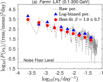
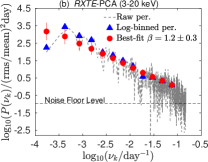
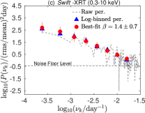
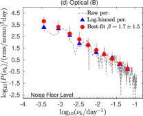
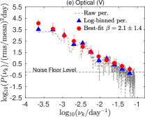
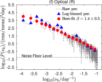
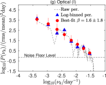
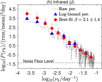
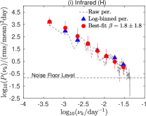
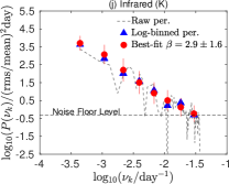
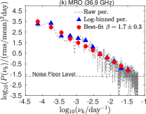
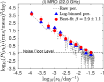
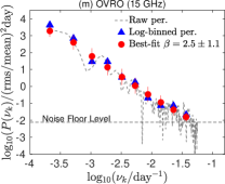
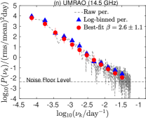
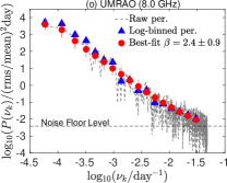
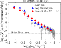
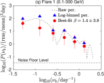
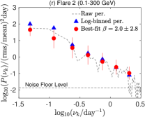
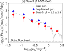
Figure 5: Best-fit PSDs of the multiwavelength light curves shown in Figures 1,  3(a, b, and c), and  4(a) for the blazar 3C 279, derived using the PSRESP method. Variability power spectrum down to the Nyquist sampling frequency of the (mean) observed data is derived. The dashed line shows the ‘raw’ periodogram while the blue triangles and red circles give the ‘logarithmically binned power spectrum’ and the best-fit power spectrum, respectively. The error on the best-fit PSD slope corresponds to a 98% confidence limit. The dashed horizontal line corresponds to the statistical noise floor level due to measurement noise.

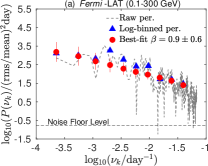
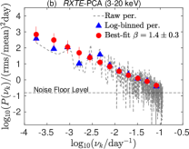
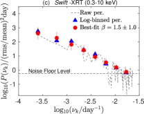
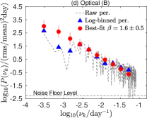
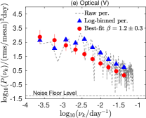
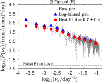
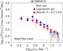
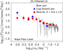
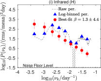
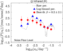
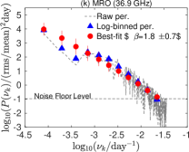
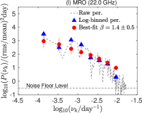
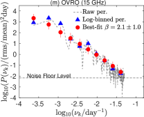
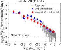
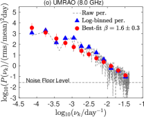
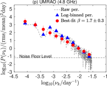
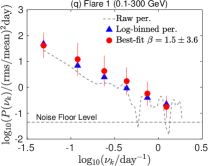
Figure 6: Best-fit PSDs of the multiwavelength light curves shown in Figures 2,  3(d), and  4(b) for the blazar PKS 1510$-$089, derived using the PSRESP method, and displayed as in Figure 5.

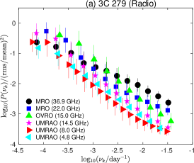
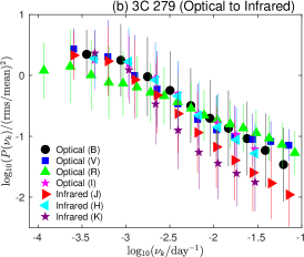
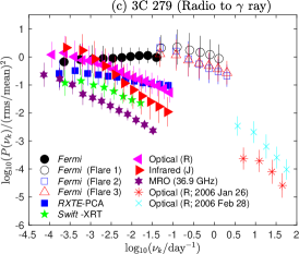
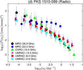
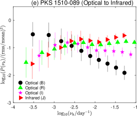
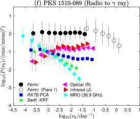
Figure 7: Square fractional variability as a function of timescale for the blazars 3C 279 (panels a, b, and c) and PKS 1510$-$089 (d, e, and f). The filled symbols show mean and standard deviation of best-fit PSDs given by the PSRESP method each frequency, while open symbols show different gamma-ray flare epochs. In panel (c) we have included the $R$-band intranight PSDs presented in Goyal (2021) for the blazar 3C 279.

4 Results

We have obtained long-term multiwavelength variability PSDs of two luminous blazars, 3C 279 and PKS 1510$-$089, using well-sampled (days/weeks sampling interval), long-duration (years–decades), datasets with good photometric accuracy ($\sim$1–15%). The variability PSDs cover $\sim$2-4 decades in temporal frequency, corresponding to decades/years/months/days timescales, depending on the waveband. The key results of our detailed analysis are as follows:

1. For both of the targets, the radio variability PSDs are best described by the single power-law shapes with confidence ranging from $\sim$14% to $\sim$97% (Column 11; Table 2). The best-fit $\beta$ range between $\sim$1.4 and $\sim$2.9 over the frequency range log₁₀$\nu_{k}$ (day^-1) between $-$4.2 and $-$1.2, indicative of flicker to red-noise type statistical characters of variability (Table 2; Figures 5 and  6). The normalizations of these radio PSDs turn out to be consistent with one another within 1–2$\sigma$ uncertainties on overlapping variability frequencies (panels (a) and (d) of Figure 7).

2. The optical and infrared variability PSDs for the blazar 3C 279 show acceptable fits to single power-law shapes with confidence in the range $\sim$56%–$\sim$99% (Column 11; Table 2). The best-fit $\beta$ values show a range between $\sim$1.4 and $\sim$2.9 over the frequency range log₁₀$\nu_{k}$ (day^-1) between $-$3.93 and $-$1.09, indicative of flicker to red-noise variability (Table 2; Figure 5). For the blazar PKS 1510$-$089, the single power-law shape of the PSDs give acceptable fits with confidence $\geq$10% to $B$, $R$, $I$, and $J$-band PSDs (Column 11; Table 2). The $\beta$s range between $\sim$0.2 and $\sim$1.5 over the frequency range log₁₀$\nu_{k}$ (day^-1) between $-$3.68 and $-$1.03, closer to flicker noise. (Table 2; Figure 6). The variability PSDs at $V$, $H$, and $K$-bands do not provide acceptable fits to single power-law shapes for the blazar PKS 1510$-$089 (Table 2; Figure 6). The normalizations of these PSDs again are consistent with one another within 1-2$\sigma$ uncertainties where the variability frequencies overlap (panels (b) and (e) of Figure 7).

3. For both blazars, the X-ray variability PSDs are well described by single power-law shapes with confidence ranging from $\sim$48% to $\sim$99% (Column 11; Table 2). The best-fit $\beta$s are between $\sim$1.2 and $\sim$1.5 over the frequency range log₁₀$\nu_{k}$ (day^-1) between $-$3.76 and $-$1.08, indicative of nearly flicker-noise variability (Table 2; Figures 5 and  6). The PSDs obtained using RXTE-PCA and Swift-XRT datasets for both of the targets complement each other well for overlapping variability frequencies (panels (c) and (f) of Figures 7).

4. For both FSRQs, the $\gamma$-ray variability PSDs are also very well described by single power-law shapes with confidence ranging from $\sim$30% to $\sim$59% (Column 11; Table 2). The best-fit $\beta$ values are $\sim$1.0 and $\sim$0.9 for the blazars 3C 279 and PKS 1510$-$089, respectively, for the frequency range log₁₀ $\nu_{k}$ (day^-1) between $-$3.64 and $-$1.40 (1-week integration bin light curves), clearly indicative of flicker-noise (Table 2; Figures 5 and  6). The short-term variability PSD slopes derived using 3-hr integration bin light curves during bright phases (and of duration 3 weeks), identified as Flare 1, Flare 2, and Flare 3 for the blazar 3C 279 and Flare 1 for the blazar PKS 1510$-$089, are $\sim$1.4, $\sim$2.0, $\sim$1.5, and $\sim$1.7, respectively, covering the frequency range log₁₀$\nu_{k}$ (day^-1) between $-1.31$ and $+0.51$ (Table 2; Figures 5 and  6). The inclusion of short-term $\gamma$-ray variability PSDs allows us to characterize the variability spectrum across four decades without any gaps for these blazars, albeit only during the flares, when the fluxes were high enough to allow measurements over those short periods. The normalizations of the short-term $\gamma$-ray variability PSDs appear to be smooth extrapolations from those at longer timescales (panels (c) and (f) of Figure 7).

5. The inclusion of $R$-band intranight PSDs from Goyal (2021) allows us to construct, for the first time, the power spectrum across $\sim$6 decades of variability frequencies for the blazar 3C 279. The normalization of intranight PSDs appears to be a smooth extrapolation from longer timescales (panel (c) of Figure 7), indicating the dominance of a single variability process operating across 6 decades of time.

6. A direct comparison of variability power over different timescales probed by our analysis indicates more power ($\geq$2$\sigma$ level) on timescales shorter than 100 days in $\gamma$-rays, as compared to radio, infrared, optical and X-ray energies for the blazar 3C 279 (panel (c) of Figure 7). The blazar PKS 1510$-$089 also exhibits more variability power on timescales shorter than 100 days in $\gamma$-ray, as compared to radio and X-ray energies (panel f of Figure 7). However, for this blazar, the variability power at optical and infrared energies is indistinguishable from those at $\gamma$-ray energies for overlapping variability frequencies (panel (f) of Figure 7).

7. The derivation of variability PSDs at multiple frequencies of the emission spectrum presented here allows us to obtain mean PSD slopes and the associated 1$\sigma$ uncertainties at two widely separated portions of the synchrotron part of the SED as well as at IC emission frequencies for the two targets (see Table 2). For 3C 279, the mean PSD slope at radio-synchrotron frequencies is 2.34$\pm$0.16 while at optical/infrared-synchrotron frequencies it is 1.95$\pm$0.22; however, at IC frequencies it is 1.20$\pm$0.15. For the blazar PKS 1510$-$089, the mean PSD slope at radio-synchrotron frequencies is 1.60$\pm$0.08, at optical/infrared-synchrotron frequencies it is 0.77$\pm$0.23, and at IC frequencies is 1.30$\pm$0.16 (Table 3). The mean $\gamma$-ray PSD slope for short-term variability turns out to be 1.60$\pm$0.70 after averaging the four PSD slope estimates for the targets (Flare 1, Flare 2, Flare 3 for 3C 279 and Flare 1 for PKS 1510$-$089). The mean PSD slopes at synchrotron frequencies and IC frequency are different from each other at the $\geq$2$\sigma$ level for the blazar 3C 279. The mean PSD slopes at synchrotron and IC frequencies turns out to be consistent with each other within 2$\sigma$ uncertainty for the blazar PKS 1510$-$089. On the whole, the synchrotron PSD slopes of 3C 279 are steeper than those of PKS 1510$-$089 while their IC PSD slopes are similar.

5 Discussion and Summary

5.1 Comparison of PSD slopes with the literature

The $\gamma$-ray PSD slopes computed with the PSRESP technique used here for the blazars 3C 279 and PKS 1510$-$089 employing the decade-long light curves are consistent with those given in previous studies ($\beta$$\sim$0.6 and $\sim$1.0 for 3C 279 and PKS 1510$-$089, respectively; Meyer et al., 2019). Nilsson et al. (2018) reported the optical $R$-band PSD slopes $\sim$1.5 and $\sim$0.9 for the blazars 3C 279 and PKS 1510$-$089, respectively which are also consistent within errors with our estimates. Chatterjee et al. (2008) reported the PSD slopes for the blazar 3C 279 at X-ray, $R$-band optical, and radio frequencies as $\sim$2.3, $\sim$1.7, and $\sim$2.3, respectively, using the decade-long RXTE-PCA data, $R$-band, and 14.5 GHz UMRAO datasets for the period 1996-2007. Note that our longer duration X-ray, optical $R$-band and 14.5 GHz light curves include datasets reported in Chatterjee et al. (2008). The X-ray PSD slope obtained in their analysis of RXTE data is significantly steeper, $\beta=2.3\pm 0.3$, as compared to our result of $1.2\pm 0.3$. Our X-ray PSD slope is corroborated by the Swift-XRT dataset over a similar timescale ($\beta=1.4\pm 0.7$); therefore, this discrepancy cannot be due to the different lengths of light curves used in Chatterjee et al. (2008) and in our analyses for the PCA data. Good matches (within uncertainty), however, are found between the optical and radio PSD slopes between our analysis and that of Chatterjee et al. (2008). Using the full-duration UMRAO light curves for both blazars, Park & Trippe (2017) reported the PSD slopes, $\beta$$\sim$2.5, $\sim$2.2, and $\sim$1.6 at 14.5 GHz, 8.0 GHz, and 4.8 GHz, respectively, for 3C 279 and $\beta$$\sim$1.5, $\sim$1.3, and $\sim$1.4 at 14.5 GHz, 8.0 GHz, and 4.8 GHz, respectively, for PKS 1510$-$089; these are consistent within errors with our results.

We note that Ryan et al. (2019) performed direct modeling of 9.5-year long, weekly-binned $\gamma$-ray light curves for a sample of blazars, including the targets studied here, using the CARMA process (Kelly et al., 2014). Their analysis revealed a break on a year-like timescale in the PSD of the blazar PKS 1510$-$089 while the PSD of 3C 279 showed no hint of a break (meaning that the relaxation timescale could be longer than the length of the time series for this source). Our PSD analysis for the blazar PKS 1510$-$089 contradicts the results of Ryan et al. (2019) in the sense that our $\gamma$-ray PSD is best-fitted with a single power-law model with a reasonably good probability ($p_{\beta}$=0.3; Table 2). For the blazar 3C 279, Ryan et al. (2019) reports no hint of a break, indicating a good match between our PSD modeling and that reported from the CARMA modeling.

5.2 Comment on reported quasi-periodicities

We now mention the reported QPOs on year-like timescales in $\gamma$-ray and optical/infrared light curves for the period 2005-2014 claimed by Sandrinelli et al. (2016) for the blazars 3C 279 ($V$, $R$, and $K$-bands) and PKS 1510$-$089 ($V$, $R$, $J$, and $K$-bands). We also use the same dataset presented in Sandrinelli et al. (2016) and supplement it with other datasets to increase the length of the analyzed light curves. Our $\gamma$-ray PSDs are well-represented by the single power-law spectral shapes with high confidence ($p_{\beta}$$\geq$0.76). Moreover, the optical/infrared PSDs of the blazar 3C 279 are represented by the single power-law spectral form adopted in our analysis with high confidence ($p_{\beta}>$0.6). For the blazar PKS 1510$-$089, the PSDs obtained at $B$, $R$, $I$, and $J$-bands are also well represented by a single power-law spectral form with decent confidence ($p_{\beta}>0.18$, meaning that the rejection confidence for the single power-law spectral shape is $<$82%). The PSDs obtained at $V$, $H$, and $K$-bands, where the data are more limited, give poor fits, with rejection confidence $\geq$95%. The single power-law PSDs obtained in our analysis argue against the presence of reported QPOs at $V$, $R$, and $K$-bands for the blazar 3C 279 and at $R$ and $J$-bands for the blazar PKS 1510$-$089. This discrepancy between our results and those of Sandrinelli et al. (2016) could arise from the use of different methods of PSD estimation (Lomb-Scargle Periodogram in their analysis vs. DFT in our analysis) as well as the longer lengths of the light curves used in our study. If a QPO were always present, a longer duration light curve should reveal a higher significance for it, but if a QPO were transitory then additional data would weaken its significance. The lack of reproducibility is not uncommon in blazar studies as many previously claimed QPOs in the literature could not be confirmed when different methods or longer duration light curves were used for periodicity analyses (for recent discussions, see Goyal et al., 2018; Covino et al., 2019; Tarnopolski et al., 2020; Covino et al., 2020; Yang et al., 2021). Further investigation of this point is beyond the scope of this paper.

5.3 Possible interpretation for different statistical characters of low and high energy variability

As the single-zone models do not explain the statistical properties of long-term multiwavelength variability adequately (Section 1), based on the different statistical characters of multiwavelength variability exhibited by the BL Lac object PKS 0735$+$178 ($\beta\sim$2 for radio/optical emissions but $\sim$1 at HE $\gamma$-ray energies), we hypothesized in Goyal et al. (2017) that the entire broadband emission is produced in an extended and turbulent jet. We noted there that these results would arise if a single stochastic process is responsible for the variability at synchrotron frequencies while a linear superposition of two or more stochastic processes with widely different relaxation timescales produce variability at IC frequencies. We speculated that the drivers behind the synchrotron variability can be stochastic fluctuations in the jet plasma conditions (such as variations in the magnetic field or bulk Lorentz factor) leading to dissipation of energy over wide spatial scales. The radiative response of the accelerated particles will be delayed with respect to the input perturbations, thereby producing the red-noise variability at synchrotron frequencies on timescales smaller than the relaxation timescales of the process. Because we did not recover the flattening of PSDs on longer timescales ($\geq$1,000 days), we noted that the driver should be related to some global magnetohydrodynamic timescale. At IC frequencies, however, due to inhomogeneities in the population of photons available for upscattering, an additional stochastic process with relaxation timescale equal to a light crossing time $\sim$1 day (a valid approximation for a boosted jet with bulk Lorentz factor 30) was envisaged. IC variability is expected to show red-noise character on timescales shorter than $\sim$day in our model. Our hypothesis was supported in Goyal (2020) where the VHE $\gamma$-rays also exhibited $\beta$$\sim$1 for the blazars Mrk 421 and PKS 2155$-$304 whose TeV emission is often concluded to be due to SSC processes (Abdo et al., 2011a; Abramowski et al., 2012; Aleksić et al., 2012; Madejski et al., 2016; Abdalla et al., 2020; Dmytriiev et al., 2021).

The best-fit PSD slopes for all of the individual emission frequencies that we report here range between $\beta$$\sim$0.2-2.9; however, the statistically significant slopes span a narrower range, 0.7 to 2.9, which correspond to flicker and red-noise statistical characters of variability. We note that in many cases, the reported 98% confidence limit on the PSD estimate is large (Table 2) which renders a strict statistical classification of the variability unfeasible. The mean PSD slopes, however, obtained at radio-synchrotron and optical-synchrotron frequencies correspond to statistical characters consistent with strict red-noise $\beta$$\sim$2 (except for PKS 1510$-$089 for which the mean $\beta$ at optical/infrared frequency is $\sim$0.8) and to a strict flicker-noise ($\beta$$\sim$1) statistical character at IC emission frequency on timescales ranging from decades/years to weeks/days. As such their broadband variability behaviors basically can be understood within our model, as summarized in the previous paragraph and given in more detail in Goyal et al. (2017).

5.4 Flicker-noise type variability at optical/IR energies of PKS 1510$-$089: jet + accretion disk

For PKS 1510$-$089 the optical/infrared variability seems to be better represented by flicker noise whenever the single power-law form was found to be an adequate fit. This is not expected within our model (Section 5.3) as the emission at optical/infrared frequencies is presumed to be dominated by synchrotron processes for such FSRQ type blazars, although the radio variability is well-represented by red-noise processes for the same source and, of course, that is synchrotron radiation. Therefore, our model cannot be considered inadequate based on the flicker-noise character at synchrotron frequencies because in such a case we expect the radio frequencies to mimic the infrared/optical frequencies.

However, the FSRQ PKS 1510$-$089 is well-known to have a prominent thermal accretion disk component in its SED at UV/infrared frequencies, not only during quiescent states but even when flaring (e.g., D’Ammando et al., 2011; Nalewajko et al., 2012; Aleksić et al., 2014; Ahnen et al., 2017); therefore, one expects different variability properties if the jet emission (as the source shows significant optical polarization variability at times; Itoh et al., 2016; Beaklini et al., 2018) is diluted by the accretion disk component. Assuming that the majority of the disk emission originates within 100  Schwarzschild radii of the accretion disk (Shakura & Sunyaev, 1976) with viscosity parameter $\alpha=0.01$, the characteristic light-crossing, gas orbital, and thermal/viscous timescales for this blazar turn out to be $\leq$1 day, $\sim$31–73 days, and $\sim$1.4–3.2 yrs, respectively (Kelly et al., 2009), for a black hole of mass range (3–7)$\times$10${{}^{7}}\,M_{\odot}$ (Table 1). Since the optical/infrared PSDs cover 6–12 yrs  down to weeks timescale, such instabilities operating on these timescales seem to be valid candidates for the production of fluctuations in the disk emission in this source (e.g., Wiita, 2006). Therefore, the flatter optical/infrared PSD slopes for this source could be reconciled if the emission at optical/infrared frequencies is driven by a linear combination of stochastic process(es) driving the disk emission at shorter timescales (days to years) and the jet emission which could include longer relaxation timescales ($\approx$1,000 days) (see, in this regard, Kelly et al., 2011; Sobolewska et al., 2014).

5.5 Relaxation/characteristic timescales

The combination of $\gamma$-ray measurements made over the long-term (obtained with 1-week integrations) and short-term (obtained with 3-hr integrations for short durations only when source fluxes were high) allowed us to characterize the $\gamma$-ray variability PSDs across 4 decades. The mean PSD slope at short timescales is consistent with those at longer timescales, within the large uncertainties of the former and as such does not require the presence of a break as apparently seen in some blazars around $\sim$days timescales (Sobolewska et al., 2014; Ryan et al., 2019). The optical PSD for the blazar 3C 279 could be characterized across 6 decades due to the inclusion of intranight PSDs on two occasions (2006 January 26 and 2006 February 28; Goyal, 2021). The continuity of normalized power spectra across 6 decades indicates that a continuous (single) stochastic process appears to drive the variability at optical frequencies.

In none of the analyzed light curves, however, do we recover the relaxation timescale of the process driving the variability, which should entail seeing $\beta$ changing from $\geq$1 to $\sim$0 at frequencies below the inverse of that timescale. The $\gamma$-ray and optical/infrared PSDs are in particular well represented by single power-law spectral shapes with high confidence up to timescales of the order of a decade or more. As the majority of HE jet emission is believed to originate at $\sim$1 pc  distance from the supermassive black hole (see, Sikora et al., 2009; Harvey et al., 2020, and references therein), the corresponding relaxation timescales for the $\gamma$-ray variability should turn out to be a few months in the observer’s frame (assuming a typical bulk Lorentz factor of 10; Lister et al., 2016). The absence of PSD breaks in these blazars implies that the $\gamma$-ray emission originates, like the optical/infrared emission, from a rather extended region, in accordance with the expectation of our hypothesis discussed in Section 5.3.

5.6 Confronting the PSD slopes with multi-zone models

The noise-like appearance of blazar light curves initiated efforts to model the jet emission due to many cells behind a shock (Marscher, 2014; Calafut & Wiita, 2015; Pollack et al., 2016). The detailed model developed by Marscher (2014) provides plausible flux light curves at both synchrotron and SSC emission frequencies but did not provide the PSDs, making a direct comparison difficult with these multiband variability observations. In contrast, the modeling done by Calafut & Wiita (2015) and Pollack et al. (2016) computes light curves as well as PSDs, but only at synchrotron emission frequencies. For relativistic hydrodynamic simulations of 2D jets where the emission and its variability are shaped by the combination of bulk Lorentz factor fluctuations and the turbulence within the jets, PSD slopes in the range 2.1 to 2.9 due to bulk Lorentz factor changes and in the range 1.7 to 2.3 due to turbulence are expected (Pollack et al., 2016). In this scenario, the majority of radio-optical PSD slopes (synchrotron emission frequencies) obtained in our study can be reconciled with those attributed primarily to changes in bulk Lorentz factors for the blazar 3C 279 and to turbulence for the blazar PKS 1510$-$089. However, such models would need to be extended to show that they naturally can produce significantly flatter PSD slopes at IC energies, before considering them actually supported by our analysis.

5.7 Key conclusions

In summary, we have explored the statistical properties of blazar light curves by means of variability PSDs using good photometric quality ($\sim$1-15% flux accuracy), extensive multiwavelength datasets ($\geq$15 different frequencies covering 13 decades of the emission spectrum) available for the blazars 3C 279 and PKS 1510$-$089 over timescales exceeding a decade. The majority of PSDs show a good fit to single power-law spectral shapes over temporal frequencies ranging between $\sim$10^-4 and $\sim$10^-1 (day^-1). However, we note that PSDs on temporal frequencies longer than 10^-2.7 (day^-1) are poorly sampled, providing only a few up to 10 cycles in the PSDs.

The mean PSD slopes at radio and optical-synchrotron emission frequencies are steeper from those at IC emission frequencies at $\geq$2$\sigma$ level on timescales ranging from decades to weeks/days for the blazar 3C 279. On similar broad timescales, the mean PSD slopes at radio and optical-synchrotron emission frequencies and at IC emission frequencies turn out to be statistically indistinguishable ($\leq$2$\sigma$ level) from one another for the blazar PKS 1510$-$089. The $\gamma$-ray variability PSDs covers $\sim$4 decades of the variability spectrum for these two blazars where the short-term variability PSDs connect smoothly to the long-term variability PSDs. The optical variability power spectrum covers $\sim$6 decades for the blazar 3C 279 and the normalization of intranight PSDs appears to be a simple extrapolation from longer timescales.

Appendix A Spectral window function of the Fourier transformation on the observed datasets

An efficient diagnostic to discern the deleterious effects of Fourier transformation on the time series is to derive its spectral window function. The spectral window function measures the response of a Fourier transformation when applied on unevenly sampled time series. Specifically, it is 1 at the zeroth Fourier frequency and 0 at other frequencies for an evenly sampled time series (e.g., Deeming, 1975; Goyal, 2020). Figures A.1 and  A.2 present the sampling distribution and the corresponding spectral window functions for the long-term light curves of 3C 279 and PKS 1510$-$089, respectively. The spectral window functions corresponding to the Fermi-LAT curves for the targets show a uniform response across the frequency range as the LAT data are precisely sampled in 1-week intervals, and the other sampling values (14 and 21 days) are due to the missing TS$<$10 data points. The majority of spectral window function curves corresponding to optical, infrared, and radio light curves exhibit broad/narrow peaks around $\sim$300 days timescale due to seasonal gaps in observation because of the source’s proximity to the Sun. The sharpness of the peak in the spectral window function depends on the number of cycles covered. Therefore, those are more prominently seen in the few decades-long MRO and UMRAO radio light curves as compared to the nearly decade-long optical and infrared light curves. The spectral window function corresponding to the RXTE-PCA and Swift-XRT datasets also shows prominent peaks around the $\sim$300 days timescale, due to the scheduling constraints of these observations with the satellites due to the position of the Sun. Moreover, as expected, the spectral window functions related to the 3-hr integration bin show a rather uniform response across the frequency range as the light curves are without any periodic gaps, like those of weekly-binned LAT light curves.

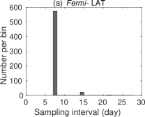
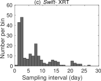
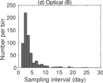
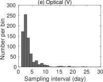
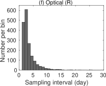
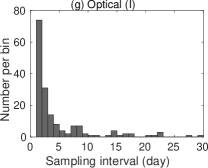
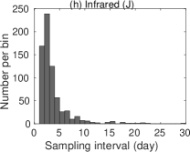
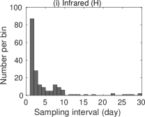
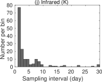
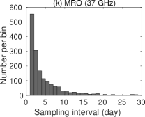
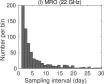
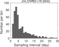
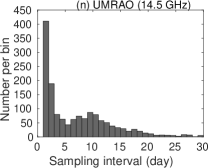
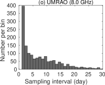
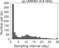
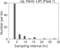
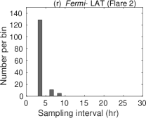
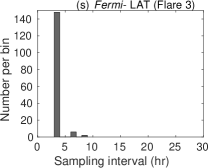
Figure A.1: Sampling distribution of the analyzed light curves (panels a-s) and the corresponding spectral window of DFT (panels a1-s1) are shown for the blazar 3C 279. Sampling intervals larger than 30 days are not shown for clarity as they usually include less than 20 data points for the $\gamma$-ray, X-ray, optical, and infrared light curves and less than 60 data points for radio light curves (except for the OVRO light curve for which it is less than 20 data points).

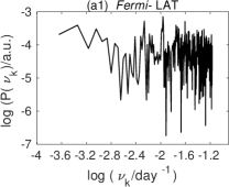
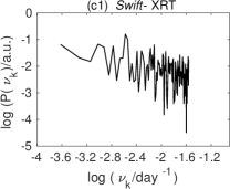
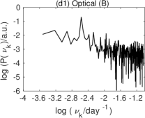
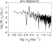
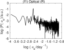
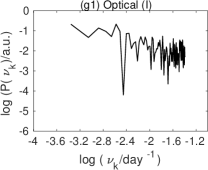
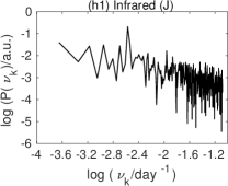
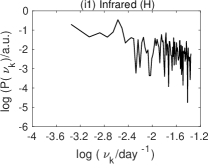
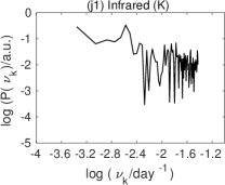
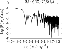
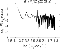
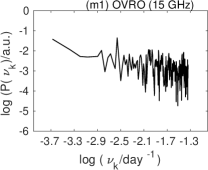
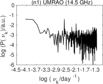
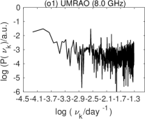
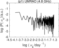
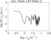
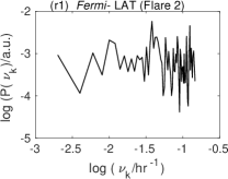
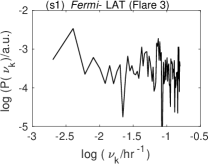
Figure A.1: (continued)

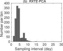
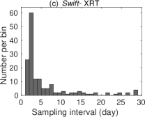
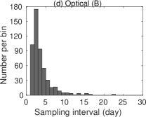
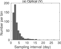
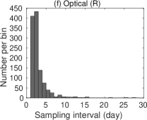
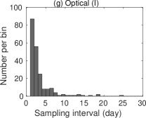
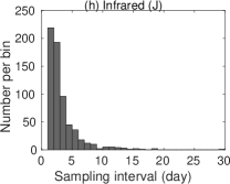
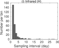
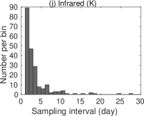
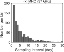
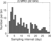
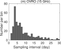
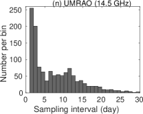
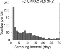
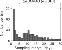
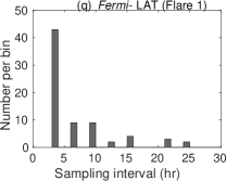
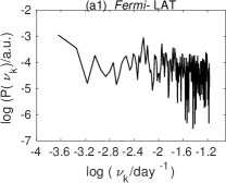
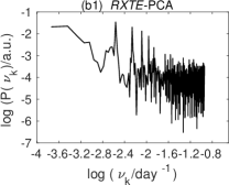
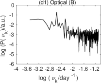
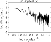
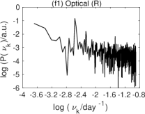
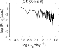
Figure A.2: As in Figure A.1, but for the blazar PKS 1510$-$089.

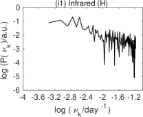
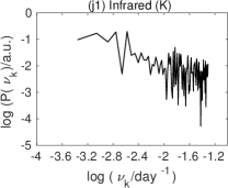
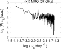
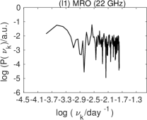
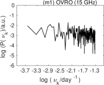
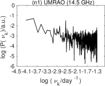
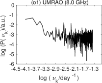
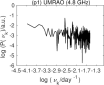
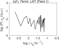
Figure A.2: (continued)

Appendix B Distribution curves of the analyzed PSDs

Figure B.1: Distribution curves for the spectral parameters investigated using the PSRESP method for the blazar 3C 279. The best-fitting value of $\beta$ is taken as the one with the highest $p_{\beta}$. The dashed curve is a Gaussian function fitted to the data with full-width at half maxima (FWHM), related to the standard deviation as 2.354$\sigma$.

Figure B.2: As in Figure B.1, for the blazar PKS 1510$-$089.

Appendix C Comparison of PSD shapes using the DFT and LSP methods

The LS periodogram (LSP) is famous for naturally handling the data gaps in the time series (Lomb, 1976; Scargle, 1982) as compared to the DFT method, which introduces spurious power in the periodogram for unevenly sampled time series (Appendix A). Therefore, to perform DFT of the unevenly sampled time series (as is the case with the observed light curves), a linear interpolation between successive data points is used to obtain an evenly sampled time series. In such cases, the periodograms are obtained down to Nyquist frequencies corresponding to the mean sampling interval of the time series, as linear interpolation introduces a “lack of variability” (relative to the intrinsic variability) into the highest frequencies. In the case of LSP, however, the periodograms can be obtained down to the highest Nyquist frequency (determined by the smallest sampling interval; VanderPlas, 2018).

With numerical simulation, however, we demonstrate that contrary to expectations, the LSP PSD does not reproduce the shape of the intrinsic PSD down to the maximum Nyquist frequency when sampling is relatively sparse. To do so, we simulated a light curve with $\beta=2$ and a log-normal flux distribution, following the method of Emmanoulopoulos et al. (2013), containing 4,000 data points with a sampling interval of one day. This length is chosen to mimic the nearly decade-long light curves studied in the present study. Using this light curve, we obtained unevenly sampled light curves with mean sampling rates equal to 10%, 25%, and 50%, respectively, in two fashions. (1) We introduced random gaps in the time series such that 90%, 75%, and 50% data were discarded at random times; these sorts of sampling patterns are expected from monitoring instruments such as Fermi-LAT when fluxes fall below the TS threshold (shown in panel (a) of Figure C.1). (2) We introduced a 3-month long systematic gap every twelve months in the time series as well as random gaps in the time series; these sorts of sampling patterns are expected at optical and infrared wavelengths from ground-based telescopes (shown in panel (b) of Figure C.1). For simplicity, we did not add Gaussian fluctuations resulting from measurement uncertainties in the simulated LCs. The $T_{\rm mean}$ values correspond to $\sim$10, $\sim$4 and $\sim$2 days, respectively, for these light curves.

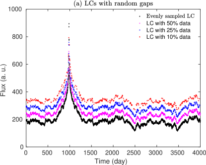
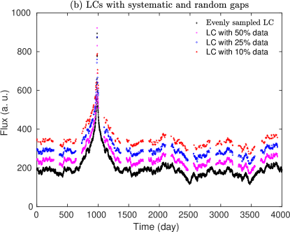
Figure C.1: Evenly sampled light curve (LC) generated with $\beta$=2 and log-normal flux distribution for a total duration of 4,000 day with a sampling interval of 1  day (black cross). Panel (a) shows the unevenly sampled light curves containing 10% (red star), 25% (blue diamond), and 50% (magenta pentagon) of the data, respectively, by introducing random gaps in the time series. Panel (b) shows the unevenly sampled light curves containing 10% (red star), 25% (blue diamond), and 50% (magenta pentagon) of the data, respectively, by introducing seasonal (3 months) and random gaps in the time series. The unevenly sampled LCs are shifted vertically for clarity of visualization.

The LSP (Scargle, 1982) of an unevenly sampled, mean-subtracted light curve $f(t_{i})$, with the total duration of $T$, consisting of $N$ data points, is defined as:

$$P_{f}(2\pi\nu_{k})=\frac{1}{2}\left\{\frac{\Bigg{\{}\sum_{i=1}^{N}f(t_{i})\cos[2\pi\nu_{k}(t_{i}-\tau)]\Bigg{\}}^{2}}{\sum_{i=1}^{N}f(t_{i})\cos^{2}[2\pi\nu_{k}(t_{i}-\tau)]}+\frac{\Bigg{\{}\sum_{i=1}^{N}f(t_{i})\sin[2\pi\nu_{k}(t_{i}-\tau)]\Bigg{\}}^{2}}{\sum_{i=1}^{N}f(t_{i})\sin^{2}[2\pi\nu_{k}(t_{i}-\tau)]}\right\}\,,$$ (C1)

where a factor $\tau$, which accounts for the uneven sampling, is defined by

$$\tau=\arctan\Bigg{\{}\frac{1}{2(2\pi\nu_{k})}\,\frac{\sum_{i=1}^{N}\sin[2(2\pi\nu_{k})t_{i}]}{\sum_{i=1}^{N}\cos[2(2\pi\nu_{k})t_{i}]}\Bigg{\}}\,,$$ (C2)

The LS program was derived for evenly spaced frequencies ranging from the total duration of the light curve, $T$, down to the maximum Nyquist sampling frequency (0.5 day^-1). Figures C.2 and  C.3 show the best-fit PSDs obtained using the PSRESP method for the DFT and LSP methods on the unevenly sampled light curves with 10%, 25%, and 50% sampling rates shown in panels (a) and (b) of Figure C.1. Moreover, to obtain the PSD using the DFT method, the unevenly sampled time series is rendered evenly sampled through linear interpolation with an interval of 0.5 day. The success fractions for the two methods are given in Figures C.4 (LCs with random gaps only) and  C.5 (LCs with systematic and random gaps), respectively. The best-fit PSD slope obtained using the LSP method for the 25% sampling rate data with the random gaps (Figure C.2e) does not have error estimation as the probability curve does not allow for fitting the Gaussian function because the success fractions turned out to be non-zero for only two $\beta$ values of the scanned range. On the other hand, we could not derive the best-fit LSP PSD using the PSRESP method for the 50% sampling rate data with systematic and random gaps because the success fraction turned out to be zero at all $\beta$ values (Figure C.3f).

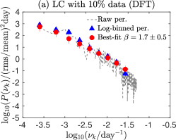
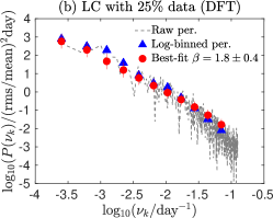
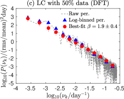
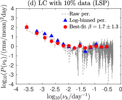
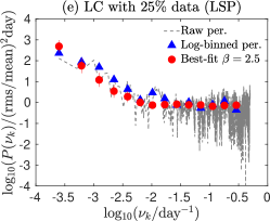
Figure C.2: The best-fit PSDs obtained for the unevenly sampled LCs shown in Figure C.1(a) using the PSRESP formalism for the DFT (panels a, b, and c) and LSP (panels d, e, and f) methods (see Section 3.2 for details). The maximum Nyquist frequencies are 1/2*$T_{\rm mean}$ (day^-1) and 0.5 (day^-1), respectively, for the DFT and the LSP methods. Note that the simulated LCs are free of noise; therefore, the flattening in the LSP PSDs on frequencies $\geq$ 10^-1.5(day^-1) arises from the small number of data points available to characterize the variability at the highest frequencies (up to the maximum Nyquist frequency).

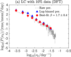
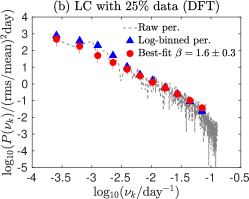
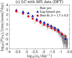
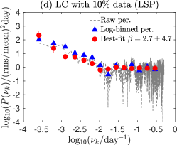
Figure C.3: The best-fit PSDs obtained for the unevenly sampled LCs shown in Figure C.1(b) using the PSRESP formalism for the DFT (panels a, b, and c) and LSP (panels d, e, and f) methods (see Section 3.2 for details). The maximum Nyquist frequencies are 1/2*$T_{\rm mean}$ (day^-1) and 0.5 (day^-1), respectively, for the DFT and the LSP methods. Note that the simulated LCs are free of noise; therefore, the flattening in the LSP PSDs on frequencies $\geq$ 10^-1.5(day^-1) arises from the small number of data points available to characterize the variability at the highest frequencies (up to the maximum Nyquist frequency).

Figures C.2 and  C.3 demonstrate that the LS periodograms do not reproduce steep power spectra in the case of unevenly sampled data. Generally speaking, in the case of the LSP method, that is because of a small number of degrees of freedom (DOF) available to characterize the variability at the highest frequencies up to the maximum Nyquist frequency. Although the derived PSD slopes using the PSRESP method ($\beta=$1.6–2.7) can be considered reasonably close to the intrinsic PSD slope ($\beta=2$), a flattening of the PSDs at higher frequencies ($\geq$10^-1.5 day^-1) is the result of the DOF issue mentioned above, which introduces artificial power in the high-frequency range of the spectrum and not because of measurement uncertainties, since the simulated light curves are free of scatter that would come from these uncertainties.

The DFT method (panels a, b, and c of Figures C.2 and  C.3), on the other hand, recovers the actual slope ($\beta$= 2) with high probability (panels a, b, and c of Figures C.4 and  C.5), without introducing additional effects in the derived power spectrum; therefore, the DFT method is the better choice between the two methods (see, also, Appendix of Goyal et al., 2017, for a relevant discussion). Furthermore, we note that the success fractions are low for the LSP PSRESP formalism, most likely due to the contribution of “extra” white noise ($\beta=$ 0) at higher frequencies, relative to the input spectrum, due to the undersampling. Finally, we reiterate that the differences in the derived power spectra using the two methods diminish gradually with a progressively increasing sampling of the light curves, with the output becoming the same for the evenly sampled time series (VanderPlas, 2018).

Figure C.4: probability curves for DFT (panels a, b, and c) and LSP (d, e, and f) methods for light curves shown in Figure C.1a.

Figure C.5: probability curves for DFT (panels a, b, and c) and LSP (d and e) methods for light curves shown in Figure C.1b.

References

- Abdalla et al. (2020) Abdalla, H., Adam, R., Aharonian, F., et al. 2020, A&A, 639, A42, doi: 10.1051/0004-6361/201936900
- Abdo et al. (2010a) Abdo, A. A., Ackermann, M., Ajello, M., et al. 2010a, ApJ, 722, 520, doi: 10.1088/0004-637X/722/1/520
- Abdo et al. (2010b) —. 2010b, Nature, 463, 919, doi: 10.1038/nature08841
- Abdo et al. (2010c) Abdo, A. A., Ackermann, M., Agudo, I., et al. 2010c, ApJ, 721, 1425, doi: 10.1088/0004-637X/721/2/1425
- Abdo et al. (2011a) Abdo, A. A., Ackermann, M., Ajello, M., et al. 2011a, ApJ, 736, 131, doi: 10.1088/0004-637X/736/2/131
- Abdo et al. (2011b) —. 2011b, ApJ, 727, 129, doi: 10.1088/0004-637X/727/2/129
- Abdo et al. (2011c) —. 2011c, ApJ, 734, 116, doi: 10.1088/0004-637X/734/2/116
- Abdo et al. (2012) —. 2012, ApJ, 758, 140, doi: 10.1088/0004-637X/758/2/140
- Abdollahi et al. (2020) Abdollahi, S., Acero, F., Ackermann, M., et al. 2020, ApJS, 247, 33, doi: 10.3847/1538-4365/ab6bcb
- Abramowski et al. (2012) Abramowski, A., Acero, F., Aharonian, F., et al. 2012, A&A, 539, A149, doi: 10.1051/0004-6361/201117509
- Ackermann et al. (2016) Ackermann, M., Anantua, R., Asano, K., et al. 2016, ApJ, 824, L20, doi: 10.3847/2041-8205/824/2/L20
- Ahnen et al. (2017) Ahnen, M. L., Ansoldi, S., Antonelli, L. A., et al. 2017, A&A, 603, A29, doi: 10.1051/0004-6361/201629960
- Aleksić et al. (2012) Aleksić, J., Alvarez, E. A., Antonelli, L. A., et al. 2012, A&A, 542, A100, doi: 10.1051/0004-6361/201117442
- Aleksić et al. (2014) Aleksić, J., Ansoldi, S., Antonelli, L. A., et al. 2014, A&A, 569, A46, doi: 10.1051/0004-6361/201423484
- Aleksić et al. (2015) —. 2015, A&A, 578, A22, doi: 10.1051/0004-6361/201424811
- Aller et al. (1985) Aller, H. D., Aller, M. F., Latimer, G. E., & Hodge, P. E. 1985, ApJS, 59, 513, doi: 10.1086/191083
- Aller et al. (1999) Aller, M. F., Aller, H. D., Hughes, P. A., & Latimer, G. E. 1999, ApJ, 512, 601, doi: 10.1086/306799
- Atwood et al. (2013) Atwood, W., Albert, A., Baldini, L., et al. 2013, arXiv e-prints, arXiv:1303.3514. https://arxiv.org/abs/1303.3514
- Atwood et al. (2009) Atwood, W. B., Abdo, A. A., Ackermann, M., et al. 2009, ApJ, 697, 1071, doi: 10.1088/0004-637X/697/2/1071
- Ballet et al. (2020) Ballet, J., Burnett, T. H., Digel, S. W., & Lott, B. 2020, arXiv e-prints, arXiv:2005.11208. https://arxiv.org/abs/2005.11208
- Barbiellini et al. (2014) Barbiellini, G., Bastieri, D., Bechtol, K., et al. 2014, ApJ, 784, 118, doi: 10.1088/0004-637X/784/2/118
- Beaklini et al. (2018) Beaklini, P., Dominici, T., & Abraham, Z. 2018, Galaxies, 6, 18, doi: 10.3390/galaxies6010018
- Bennett et al. (2014) Bennett, C. L., Larson, D., Weiland, J. L., & Hinshaw, G. 2014, ApJ, 794, 135, doi: 10.1088/0004-637X/794/2/135
- Bevington & Robinson (2003) Bevington, P. R., & Robinson, D. K. 2003, Data reduction and error analysis for the physical sciences (3rd ed., by Philip R. Bevington, and Keith D. Robinson. Boston, MA: McGraw-Hill, ISBN 0-07-247227-8, 2003)
- Bhatta & Dhital (2020) Bhatta, G., & Dhital, N. 2020, ApJ, 891, 120, doi: 10.3847/1538-4357/ab7455
- Bhatta et al. (2016a) Bhatta, G., Stawarz, Ł., Ostrowski, M., et al. 2016a, ApJ, 831, 92, doi: 10.3847/0004-637X/831/1/92
- Bhatta et al. (2016b) Bhatta, G., Zola, S., Stawarz, Ł., et al. 2016b, ApJ, 832, 47, doi: 10.3847/0004-637X/832/1/47
- Bhattacharyya et al. (2020) Bhattacharyya, S., Ghosh, R., Chatterjee, R., & Das, N. 2020, ApJ, 897, 25, doi: 10.3847/1538-4357/ab91a8
- Blandford et al. (2019) Blandford, R., Meier, D., & Readhead, A. 2019, ARA&A, 57, 467, doi: 10.1146/annurev-astro-081817-051948
- Bonning et al. (2012) Bonning, E., Urry, C. M., Bailyn, C., et al. 2012, ApJ, 756, 13, doi: 10.1088/0004-637X/756/1/13
- Böttcher et al. (2013) Böttcher, M., Reimer, A., Sweeney, K., & Prakash, A. 2013, ApJ, 768, 54, doi: 10.1088/0004-637X/768/1/54
- Böttcher et al. (2007) Böttcher, M., Basu, S., Joshi, M., et al. 2007, ApJ, 670, 968, doi: 10.1086/522583
- Bruel et al. (2018) Bruel, P., Burnett, T. H., Digel, S. W., et al. 2018, arXiv e-prints, arXiv:1810.11394. https://arxiv.org/abs/1810.11394
- Calafut & Wiita (2015) Calafut, V., & Wiita, P. J. 2015, Journal of Astrophysics and Astronomy, 36, 255, doi: 10.1007/s12036-015-9324-2
- Castignani et al. (2013) Castignani, G., Haardt, F., Lapi, A., et al. 2013, A&A, 560, A28, doi: 10.1051/0004-6361/201321424
- Castignani et al. (2017) Castignani, G., Pian, E., Belloni, T. M., et al. 2017, A&A, 601, A30, doi: 10.1051/0004-6361/201629775
- Chatterjee et al. (2018) Chatterjee, R., Roychowdhury, A., Chandra, S., & Sinha, A. 2018, ApJ, 859, L21, doi: 10.3847/2041-8213/aac48a
- Chatterjee et al. (2008) Chatterjee, R., Jorstad, S. G., Marscher, A. P., et al. 2008, ApJ, 689, 79, doi: 10.1086/592598
- Chatterjee et al. (2012) Chatterjee, R., Bailyn, C. D., Bonning, E. W., et al. 2012, ApJ, 749, 191, doi: 10.1088/0004-637X/749/2/191
- Chen et al. (2012) Chen, X., Fossati, G., Böttcher, M., & Liang, E. 2012, MNRAS, 424, 789, doi: 10.1111/j.1365-2966.2012.21283.x
- Chen et al. (2016) Chen, X., Pohl, M., Böttcher, M., & Gao, S. 2016, MNRAS, 458, 3260, doi: 10.1093/mnras/stw528
- Chiaberge & Ghisellini (1999) Chiaberge, M., & Ghisellini, G. 1999, MNRAS, 306, 551, doi: 10.1046/j.1365-8711.1999.02538.x
- Covino et al. (2020) Covino, S., Landoni, M., Sandrinelli, A., & Treves, A. 2020, ApJ, 895, 122, doi: 10.3847/1538-4357/ab8bd4
- Covino et al. (2019) Covino, S., Sandrinelli, A., & Treves, A. 2019, MNRAS, 482, 1270, doi: 10.1093/mnras/sty2720
- Cutini (2015) Cutini, S. 2015, The Astronomer’s Telegram, 7633, 1
- D’Ammando et al. (2011) D’Ammando, F., Raiteri, C. M., Villata, M., et al. 2011, A&A, 529, A145, doi: 10.1051/0004-6361/201016128
- Deeming (1975) Deeming, T. J. 1975, Ap&SS, 36, 137, doi: 10.1007/BF00681947
- Dmytriiev et al. (2021) Dmytriiev, A., Sol, H., & Zech, A. 2021, MNRAS, 505, 2712, doi: 10.1093/mnras/stab1445
- Dutka et al. (2017) Dutka, M. S., Carpenter, B. D., Ojha, R., et al. 2017, ApJ, 835, 182, doi: 10.3847/1538-4357/835/2/182
- Emmanoulopoulos et al. (2013) Emmanoulopoulos, D., McHardy, I. M., & Papadakis, I. E. 2013, MNRAS, 433, 907, doi: 10.1093/mnras/stt764
- Finke & Becker (2014) Finke, J. D., & Becker, P. A. 2014, ApJ, 791, 21, doi: 10.1088/0004-637X/791/1/21
- Foschini et al. (2011) Foschini, L., Ghisellini, G., Tavecchio, F., Bonnoli, G., & Stamerra, A. 2011, A&A, 530, A77, doi: 10.1051/0004-6361/201117064
- Gaur et al. (2018) Gaur, H., Mohan, P., Wierzcholska, A., & Gu, M. 2018, MNRAS, 473, 3638, doi: 10.1093/mnras/stx2553
- Gehrels et al. (2004) Gehrels, N., Chincarini, G., Giommi, P., et al. 2004, ApJ, 611, 1005, doi: 10.1086/422091
- Glass (1999) Glass, I. S. 1999, Handbook of Infrared Astronomy, ed. R. Ellis, J. Huchra, S. Kahn, G. Rieke, & P. B. Stetson (Cambridge University Press, Aug 13, 1999, page 63)
- Goyal (2020) Goyal, A. 2020, MNRAS, 494, 3432, doi: 10.1093/mnras/staa997
- Goyal (2021) —. 2021, ApJ, 909, 39, doi: 10.3847/1538-4357/abd7fb
- Goyal et al. (2017) Goyal, A., Stawarz, Ł., Ostrowski, M., et al. 2017, ApJ, 837, 127, doi: 10.3847/1538-4357/aa6000
- Goyal et al. (2018) Goyal, A., Stawarz, Ł., Zola, S., et al. 2018, ApJ, 863, 175, doi: 10.3847/1538-4357/aad2de
- Gupta et al. (2019) Gupta, A. C., Tripathi, A., Wiita, P. J., et al. 2019, MNRAS, 484, 5785, doi: 10.1093/mnras/stz395
- H. E. S. S. Collaboration et al. (2013) H. E. S. S. Collaboration, Abramowski, A., Acero, F., et al. 2013, A&A, 554, A107, doi: 10.1051/0004-6361/201321135
- Hartman et al. (1992) Hartman, R. C., Bertsch, D. L., Fichtel, C. E., et al. 1992, ApJ, 385, L1, doi: 10.1086/186263
- Hartman et al. (2001) Hartman, R. C., Villata, M., Balonek, T. J., et al. 2001, ApJ, 558, 583, doi: 10.1086/322462
- Harvey et al. (2020) Harvey, A. L. W., Georganopoulos, M., & Meyer, E. T. 2020, Nature Communications, 11, 5475, doi: 10.1038/s41467-020-19296-6
- Hayashida et al. (2012) Hayashida, M., Madejski, G. M., Nalewajko, K., et al. 2012, ApJ, 754, 114, doi: 10.1088/0004-637X/754/2/114
- Hayashida et al. (2015) Hayashida, M., Nalewajko, K., Madejski, G. M., et al. 2015, ApJ, 807, 79, doi: 10.1088/0004-637X/807/1/79
- Hovatta & Lindfors (2019) Hovatta, T., & Lindfors, E. 2019, New A Rev., 87, 101541, doi: 10.1016/j.newar.2020.101541
- Hu et al. (2021) Hu, W., Yan, D.-h., & Hu, Q.-l. 2021, arXiv e-prints, arXiv:2102.07328. https://arxiv.org/abs/2102.07328
- Hungwe et al. (2011) Hungwe, F., Dutka, M., & Ojha, R. 2011, The Astronomer’s Telegram, 3694, 1
- Isobe et al. (2015) Isobe, N., Sato, R., Ueda, Y., et al. 2015, ApJ, 798, 27, doi: 10.1088/0004-637X/798/1/27
- Itoh et al. (2016) Itoh, R., Nalewajko, K., Fukazawa, Y., et al. 2016, ApJ, 833, 77, doi: 10.3847/1538-4357/833/1/77
- Johannesson & Orlando (2013) Johannesson, G., & Orlando, E. 2013, in International Cosmic Ray Conference, Vol. 33, International Cosmic Ray Conference, 3106. https://arxiv.org/abs/1307.0197
- Jorstad & Marscher (2016) Jorstad, S., & Marscher, A. 2016, Galaxies, 4, 47, doi: 10.3390/galaxies4040047
- Kalberla et al. (2005) Kalberla, P. M. W., Burton, W. B., Hartmann, D., et al. 2005, A&A, 440, 775, doi: 10.1051/0004-6361:20041864
- Kastendieck et al. (2011) Kastendieck, M. A., Ashley, M. C. B., & Horns, D. 2011, A&A, 531, A123, doi: 10.1051/0004-6361/201015918
- Kataoka et al. (2001) Kataoka, J., Takahashi, T., Wagner, S. J., et al. 2001, ApJ, 560, 659, doi: 10.1086/322442
- Kelly et al. (2009) Kelly, B. C., Bechtold, J., & Siemiginowska, A. 2009, ApJ, 698, 895, doi: 10.1088/0004-637X/698/1/895
- Kelly et al. (2014) Kelly, B. C., Becker, A. C., Sobolewska, M., Siemiginowska, A., & Uttley, P. 2014, ApJ, 788, 33, doi: 10.1088/0004-637X/788/1/33
- Kelly et al. (2011) Kelly, B. C., Sobolewska, M., & Siemiginowska, A. 2011, ApJ, 730, 52, doi: 10.1088/0004-637X/730/1/52
- Kushwaha et al. (2017) Kushwaha, P., Sinha, A., Misra, R., Singh, K. P., & de Gouveia Dal Pino, E. M. 2017, ApJ, 849, 138, doi: 10.3847/1538-4357/aa8ef5
- Kushwaha et al. (2018) Kushwaha, P., Gupta, A. C., Wiita, P. J., et al. 2018, MNRAS, 473, 1145, doi: 10.1093/mnras/stx2394
- Larionov et al. (2008a) Larionov, V. M., Jorstad, S. G., Marscher, A. P., et al. 2008a, A&A, 492, 389, doi: 10.1051/0004-6361:200810937
- Larionov et al. (2008b) —. 2008b, A&A, 492, 389, doi: 10.1051/0004-6361:200810937
- Larionov et al. (2020) —. 2020, MNRAS, 492, 3829, doi: 10.1093/mnras/staa082
- Li et al. (2021) Li, X.-P., Cai, Y., Yang, H.-T., et al. 2021, MNRAS, 506, 1540, doi: 10.1093/mnras/stab1834
- Lindfors et al. (2005) Lindfors, E. J., Valtaoja, E., & Türler, M. 2005, A&A, 440, 845, doi: 10.1051/0004-6361:20040196
- Lister et al. (2016) Lister, M. L., Aller, M. F., Aller, H. D., et al. 2016, AJ, 152, 12, doi: 10.3847/0004-6256/152/1/12
- Lomb (1976) Lomb, N. R. 1976, Ap&SS, 39, 447, doi: 10.1007/BF00648343
- Madejski & Sikora (2016) Madejski, G. ., & Sikora, M. 2016, ARA&A, 54, 725, doi: 10.1146/annurev-astro-081913-040044
- Madejski et al. (2016) Madejski, G. M., Nalewajko, K., Madsen, K. K., et al. 2016, ApJ, 831, 142, doi: 10.3847/0004-637X/831/2/142
- MAGIC Collaboration et al. (2008) MAGIC Collaboration, Albert, J., Aliu, E., et al. 2008, Science, 320, 1752, doi: 10.1126/science.1157087
- Marscher (2014) Marscher, A. P. 2014, ApJ, 780, 87, doi: 10.1088/0004-637X/780/1/87
- Marscher et al. (2010) Marscher, A. P., Jorstad, S. G., Larionov, V. M., et al. 2010, ApJ, 710, L126, doi: 10.1088/2041-8205/710/2/L126
- Marziani et al. (1996) Marziani, P., Sulentic, J. W., Dultzin-Hacyan, D., Calvani, M., & Moles, M. 1996, ApJS, 104, 37, doi: 10.1086/192291
- Mattox et al. (1996) Mattox, J. R., Bertsch, D. L., Chiang, J., et al. 1996, ApJ, 461, 396, doi: 10.1086/177068
- Max-Moerbeck et al. (2014) Max-Moerbeck, W., Richards, J. L., Hovatta, T., et al. 2014, MNRAS, 445, 437, doi: 10.1093/mnras/stu1707
- Meyer et al. (2019) Meyer, M., Scargle, J. D., & Blandford, R. D. 2019, ApJ, 877, 39, doi: 10.3847/1538-4357/ab1651
- Nalewajko et al. (2012) Nalewajko, K., Sikora, M., Madejski, G. M., et al. 2012, ApJ, 760, 69, doi: 10.1088/0004-637X/760/1/69
- NASA/IPAC Extragalactic Database (2019) (NED) NASA/IPAC Extragalactic Database (NED). 2019, NASA/IPAC Extragalactic Database (NED), IPAC, doi: 10.26132/NED1
- Nilsson et al. (2018) Nilsson, K., Lindfors, E., Takalo, L. O., et al. 2018, A&A, 620, A185, doi: 10.1051/0004-6361/201833621
- Ojha & van Zyl (2018) Ojha, R., & van Zyl, P. 2018, The Astronomer’s Telegram, 11542, 1
- Orienti et al. (2013) Orienti, M., Koyama, S., D’Ammando, F., et al. 2013, MNRAS, 428, 2418, doi: 10.1093/mnras/sts201
- Paliya et al. (2015) Paliya, V. S., Sahayanathan, S., & Stalin, C. S. 2015, ApJ, 803, 15, doi: 10.1088/0004-637X/803/1/15
- Papadakis & Lawrence (1993) Papadakis, I. E., & Lawrence, A. 1993, MNRAS, 261, 612, doi: 10.1093/mnras/261.3.612
- Park & Trippe (2017) Park, J., & Trippe, S. 2017, ApJ, 834, 157, doi: 10.3847/1538-4357/834/2/157
- Pollack et al. (2016) Pollack, M., Pauls, D., & Wiita, P. J. 2016, ApJ, 820, 12, doi: 10.3847/0004-637X/820/1/12
- Press (1978) Press, W. H. 1978, Comments on Astrophysics, 7, 103
- Press et al. (1992) Press, W. H., Teukolsky, S. A., Vetterling, W. T., & Flannery, B. P. 1992, Numerical recipes in C. The art of scientific computing (2nd ed. Cambridge Univ. Press, Cambridge)
- Rakshit (2020) Rakshit, S. 2020, A&A, 642, A59, doi: 10.1051/0004-6361/202038324
- Rani et al. (2010) Rani, B., Gupta, A. C., Joshi, U. C., Ganesh, S., & Wiita, P. J. 2010, ApJ, 719, L153, doi: 10.1088/2041-8205/719/2/L153
- Rani et al. (2009) Rani, B., Wiita, P. J., & Gupta, A. C. 2009, ApJ, 696, 2170, doi: 10.1088/0004-637X/696/2/2170
- Richards et al. (2011) Richards, J. L., Max-Moerbeck, W., Pavlidou, V., et al. 2011, ApJS, 194, 29, doi: 10.1088/0067-0049/194/2/29
- Ryan et al. (2019) Ryan, J. L., Siemiginowska, A., Sobolewska, M. A., & Grindlay, J. 2019, ApJ, 885, 12, doi: 10.3847/1538-4357/ab426a
- Saito et al. (2015) Saito, S., Stawarz, Ł., Tanaka, Y. T., et al. 2015, ApJ, 809, 171, doi: 10.1088/0004-637X/809/2/171
- Sandrinelli et al. (2016) Sandrinelli, A., Covino, S., Dotti, M., & Treves, A. 2016, AJ, 151, 54, doi: 10.3847/0004-6256/151/3/54
- Sandrinelli et al. (2017) Sandrinelli, A., Covino, S., Treves, A., et al. 2017, A&A, 600, A132, doi: 10.1051/0004-6361/201630288
- Sbarrato et al. (2016) Sbarrato, T., Ghisellini, G., Tagliaferri, G., et al. 2016, MNRAS, 462, 1542, doi: 10.1093/mnras/stw1730
- Scargle (1982) Scargle, J. D. 1982, ApJ, 263, 835, doi: 10.1086/160554
- Shakura & Sunyaev (1976) Shakura, N. I., & Sunyaev, R. A. 1976, MNRAS, 175, 613
- Shukla & Mannheim (2020) Shukla, A., & Mannheim, K. 2020, Nature Communications, 11, 4176, doi: 10.1038/s41467-020-17912-z
- Sikora et al. (2009) Sikora, M., Stawarz, Ł., Moderski, R., Nalewajko, K., & Madejski, G. M. 2009, ApJ, 704, 38, doi: 10.1088/0004-637X/704/1/38
- Sobolewska et al. (2014) Sobolewska, M. A., Siemiginowska, A., Kelly, B. C., & Nalewajko, K. 2014, ApJ, 786, 143, doi: 10.1088/0004-637X/786/2/143
- Takalo et al. (2008) Takalo, L. O., Nilsson, K., Lindfors, E., et al. 2008, in American Institute of Physics Conference Series, Vol. 1085, American Institute of Physics Conference Series, ed. F. A. Aharonian, W. Hofmann, & F. Rieger, 705–707, doi: 10.1063/1.3076774
- Tarnopolski et al. (2020) Tarnopolski, M., Żywucka, N., Marchenko, V., & Pascual-Granado, J. 2020, ApJS, 250, 1, doi: 10.3847/1538-4365/aba2c7
- Teraesranta et al. (1998) Teraesranta, H., Tornikoski, M., Mujunen, A., et al. 1998, A&AS, 132, 305, doi: 10.1051/aas:1998297
- Thompson et al. (1990) Thompson, D. J., Djorgovski, S., & de Carvalho, R. 1990, PASP, 102, 1235, doi: 10.1086/132758
- Timmer & Koenig (1995) Timmer, J., & Koenig, M. 1995, A&A, 300, 707
- Ulrich et al. (1997) Ulrich, M.-H., Maraschi, L., & Urry, C. M. 1997, ARA&A, 35, 445, doi: 10.1146/annurev.astro.35.1.445
- Uttley et al. (2002) Uttley, P., McHardy, I. M., & Papadakis, I. E. 2002, MNRAS, 332, 231, doi: 10.1046/j.1365-8711.2002.05298.x
- van Zyl & Ojha (2018) van Zyl, P., & Ojha, R. 2018, The Astronomer’s Telegram, 11189, 1
- VanderPlas (2018) VanderPlas, J. T. 2018, ApJS, 236, 16, doi: 10.3847/1538-4365/aab766
- Vaughan (2005) Vaughan, S. 2005, A&A, 431, 391, doi: 10.1051/0004-6361:20041453
- Vaughan et al. (2003) Vaughan, S., Edelson, R., Warwick, R. S., & Uttley, P. 2003, MNRAS, 345, 1271, doi: 10.1046/j.1365-2966.2003.07042.x
- Wiita (2006) Wiita, P. J. 2006, in Astronomical Society of the Pacific Conference Series, Vol. 350, Blazar Variability Workshop II: Entering the GLAST Era, ed. H. R. Miller, K. Marshall, J. R. Webb, & M. F. Aller, 183
- Wright (2006) Wright, E. L. 2006, PASP, 118, 1711, doi: 10.1086/510102
- Yang et al. (2021) Yang, S., Yan, D., Zhang, P., Dai, B., & Zhang, L. 2021, ApJ, 907, 105, doi: 10.3847/1538-4357/abcbff
- Zerbi et al. (2001) Zerbi, R. M., Chincarini, G., Ghisellini, G., et al. 2001, Astronomische Nachrichten, 322, 275, doi: 10.1002/1521-3994(200112)322:5/6<275::AID-ASNA275>3.0.CO;2-N
- Żywucka et al. (2020) Żywucka, N., Tarnopolski, M., Böttcher, M., Stawarz, Ł., & Marchenko, V. 2020, ApJ, 888, 107, doi: 10.3847/1538-4357/ab5fe5