Transformaly - Two (Feature Spaces) Are Better Than One
Abstract
Anomaly detection is a well-established research area that seeks to identify samples outside of a predetermined distribution. An anomaly detection pipeline is comprised of two main stages: (1) feature extraction and (2) normality score assignment. Recent papers used pre-trained networks for feature extraction achieving state-of-the-art results. However, the use of pre-trained networks does not fully-utilize the normal samples that are available at train time. This paper suggests taking advantage of this information by using teacher-student training. In our setting, a pre-trained teacher network is used to train a student network on the normal training samples. Since the student network is trained only on normal samples, it is expected to deviate from the teacher network in abnormal cases. This difference can serve as a complementary representation to the pre-trained feature vector. Our method - - exploits a pre-trained Vision Transformer (ViT) to extract both feature vectors: the pre-trained (agnostic) features and the teacher-student (fine-tuned) features. We report state-of-the-art AUROC results in both the common unimodal setting, where one class is considered normal and the rest are considered abnormal, and the multimodal setting, where all classes but one are considered normal, and just one class is considered abnormal111The code is available at https://github.com/MatanCohen1/Transformaly.
1 Introduction
Anomaly detection is a long-standing field of research that has many applications in computer vision. The realm of anomaly detection is broad and involves different types of problems.
In the case of multi-class classification, the term ”Anomaly Detection” is often used to describe out-of-distribution (OOD) detection or novelty detection; where the task is to determine at inference time, if a test sample belongs to one of the classes the model was trained to classify or not. This task relies on what is known as the open-set assumption, where the class of a query sample can be outside the set of classes used in training.
Aside from OOD detection, one can consider two anomaly detection variants: (i) semantic anomaly detection, in which the normal and the abnormal samples differ in their semantic meaning; (ii) defect detection, in which the normal and the abnormal samples differ in their local appearance (i.e., defect), but are semantically identical. We consider the case of semantic anomaly detection.
At a high level, anomaly detection involves the combination of representation and modelling. Solutions to the problem can be divided into three categories: the unsupervised approach, the self-supervised approach and the pretrained-based approach.
Unsupervised methods use only normal data, without any form of labeling. These methods include methods for reconstructing the normal data [14, 45, 48, 25, 11], estimating its density [15], or concentrating it into one manifold [34, 36, 40].
In the self-supervised approach, a model is trained on an auxiliary task. Hopefully, the model learns meaningful features that reflect the normal nature of the data. The construction of an auxiliary task that motivates the model to learn these relevant features is not trivial, and several suggestions have been made such as geometric transformations classification [16], rotation classification [22], puzzle-solving [35] and CutPaste [24].
Recently, significant progress has been made in the self-supervised domain, with the use of contrastive learning [41, 18, 17]. Studies have shown that contrastive learning can be useful for semantic anomaly detection and produce good results [39, 38].
The combination of feature extraction from a pre-trained model and simple scoring algorithm on top of it, is an effective approach for anomaly detection [5, 22, 47]. Bergman et al. [5] used a pre-trained ResNet model, and applied a NN scoring method on the extracted features. That alone surpassed almost all unsupervised and self-supervised methods. Fine-tuning the model using either center loss or contrastive learning, leads to even better results [31, 32].
On the downside, pre-trained features are agnostic to the normal data that is available at the training stage. It is a loss of valuable information, and we propose to address it by using teacher-student training. Specifically, our work combines both pre-trained features and teacher-student training. In both cases, we use a pre-trained Vision Transformer (ViT) network as our backbone [13].
Teacher-student training was already used for pixel-precise anomaly segmentation in high resolution images [8]. Their representation learns low level statistics that are suitable for defect detection tasks. They report results that are considerably sub-par for the case of semantic anomaly detection.
We, on the other hand, focus on semantic anomaly detection, where semantic representation is crucial. In contrast to [8], we utilize not only the teacher-student discrepancy representation, but also the raw pre-trained embedding, achieving SOTA results in detecting semantic anomalies.
We modify the standard teacher-student setting by using blocks instead of the entire network. Specifically, we use the Vision-Transformer architecture (ViT) and exploit the nature of its block structure. We construct a student block that corresponds to each block of the teacher backbone. At train time, each student block is trained to mimic its corresponding teacher block. The student blocks are trained independently, and are exposed only to normal samples. At test time, each sample is represented by a vector of the differences between the teachers’ outputs and the students’ outputs. We term this representation teacher-student discrepancy.
Figure 1 gives a high-level overview of our approach. Each sample is mapped to two different feature spaces: one created by a pre-trained ViT network (the agnostic features) and another created by the discrepancy between student and teacher blocks (fine-tuned features).
The likelihood of a sample is taken to be the product of its likelihood in both feature spaces. To model the likelihoods we experimented with several options that include NN, a single Gaussian, and a Gaussian Mixture Model.
We evaluate our method on several data sets, and find that in most cases this combined representation outperforms existing state-of-the-art methods. The main contributions of this paper are:
-
•
Transformaly - a first use of dual feature representation for anomaly detection: agnostic and fine-tuned.
-
•
A novel use of teacher-student differences using Visual Transformers (ViT) for semantic anomaly detection.
-
•
State of the art results on multiple datasets and multiple settings: Cutting the error by on competitive benchmarks.
-
•
We are the first to report a hard-to-detect failure in the common unimodal setting, which we called ”Pretraining Confusion”, justify our additional multimodel evaluation process.
2 Background
The term “Anomaly Detection” encapsulate several different tasks in the literature. It has been used to describe Out-of-Distribution Detection, Defect Detection, and Semantic Anomaly Detection (the topic of this work). We will briefly cover these tasks here.
Out Of Distribution Detection:
Out-of-distribution (OOD) detection, also known as novelty detection, considers the case of multi-class classification. In this task, in addition to training an accurate model, we would also like to detect when it encounters a sample that does not belong to any of the known classes.
Several approaches took advantage of the power of supervised multi-class classification. For example, the model predictions of out-of-distribution samples have lower values than those of in-distribution samples, making anomaly detection possible [19]. Another notable approach has shown that the gap between temperature-scaled softmax scores of a sample and a perturbed version of it can be measured and used as a normality score [26]. It turns out that a larger gap is apparent in anomalous samples than in normal ones.
Defect Detection:
In defect detection the normal and the abnormal samples differ in local appearance, but are semantically identical. For example, defects in printed circuits, cables or medicinal pills.
Researchers proposed several approaches for defect detection [42, 7, 8]. Two recent papers use the Vision Transformer (ViT) architecture; Mishra et al. [28] suggest using encoder-decoder architecture in order to reconstruct the normal data. Pirany and Chai [30] proposed to train ViT using the auxiliary task of patch-inpainting. At inference time both methods use the discrepancy between the input image patches and the reconstructed image patches as an indication of possible defects.
Neither of these solutions includes a pre-training phase for the ViT. Both are best suited to detecting local defects reflected in patches, not semantic anomalies.
Bergmann et al. [8] suggested a teacher-student architecture for defect detection. The teacher model is based on a ResNet model pre-trained on a large dataset of patches from natural images. Then, an ensemble of student networks is trained on anomaly-free training data using regression loss with the teacher’s ultimate outputs.
This patch-based method is suited for defect detection, where the anomaly is in appearance and not semantic. Furthermore, this method uses only the last layer outputs for the teacher-student mechanism, and does not utilize the semantic embedding of the pre-trained network. Transformaly, on the other hand, takes advantage of different blocks in the model, by training the student blocks using intermediate outputs. Additionally, the semantically pre-trained embedding is used along with fine-tuned embedding to obtain SOTA results.
Semantic Anomaly Detection:
We can classify semantic anomaly detection solutions into three categories: Unsupervised Learning, self-supervised, and pretrained-based approaches.
Unsupervised anomaly detection solutions fall into three approaches: reconstruction-based, density estimation, and one-class classifiers.
Reconstruction-based methods attempt to capture the main characteristics of a normal training set by measuring reconstruction success. By assuming that only normal data will reconstruct well at test time, these methods attempt to detect anomalies. Previous papers have suggested nearest neighbors (-NN) [14], autoencoder [45] and GANs [48, 25, 11] in order to reconstruct and classify the samples.
Density-based methods estimate the density of the normal data. These methods predict the samples’ likelihood as their normality scores. Previous papers suggested parametric density estimation, such as mixture of Gaussians (GMM) [15], and nonparametric, such as -NN [29].
One-class classification methods map normal data to a manifold, leaving the abnormal samples outside. A few modifications have been made to SVM to adjust it for this purpose, with training only on one class [34, 36, 40].
Self-supervised methods use auxiliary tasks in order to learn relevant features of the normal data. These methods train a neural network to solve an unrelated task, using just the normal training data. At inference time, the model’s auxiliary task performance on the test set is considered as its normality score.
A number of papers have proposed applying transformations to the normal data and predicting which transformations have been applied. Predicting predefined geometric transformations [16], rotation [22], puzzle-solving [35] and CutPaste [24] are a few of the auxiliary tasks that have been suggested. In addition, (random) general transformations can be applied not only to images but also to tabular data, enabling anomalies to be detected in this domain as well [6].
Recent papers demonstrate the effectiveness of contrastive learning as a self-supervised method for learning visual representations, achieving SOTA results [9, 18, 17]. A contrastive learning approach, such as SimCLR, produces uniformly distributed outputs, making anomalies difficult to spot [9, 38]. Using contrasting shifted instances, along with rotation or transformation prediction, managed to surpass this challenge and achieved high performance [39]. Additionally, training a feature extractor using shifted contrastive learning and applying one class classification or kernel density estimation has been shown to be effective for anomaly detection [38].
Pretrained-based methods use backbones that are trained on large datasets, such as ImageNet, to extract features [12]. While in the past obtaining pre-trained models was a limitation; these days they are readily available and commonly used across many domains. These pre-trained models produce separable semantic embeddings and, as a result, enable the detection of anomalies by using simple scoring methods such as -NN or Gaussian Mixture Model [5, 47].
Surprisingly, the embeddings produced by these algorithms lead to good results also on datasets that are drastically different from the pretraining one. A follow-up paper improves the pre-training model detection performance by fine tuning it using center loss [31]. Recent publication has suggested to fine-tuned the pre-trained network using an additional dataset as outlier exposure, to further boost the results [10].
3 Method
We exploit the power of pre-trained ViT by constructing two features spaces for each sample; the pre-trained and the fine-tuned. A sample is embedded into a pre-trained feature vector and a fine-tuned feature vector .
Pre-trained Features
The pre-trained vector is obtained by passing the input through a pre-trained ViT network. This produces an embedding that is agnostic to the actual normal and abnormal data at hand.
We set and fit a Gaussian to it. At inference time, each sample is scored according its log probability as induced by the fitted model. Normal samples are assumed to have higher probability than abnormal samples.
Fine-tuned features
The fine-tune feature embedding is inspired by the knowledge distillation domain [44]. It is calculate as the difference between the output of a teacher and student ViT blocks. Specifically, we train the student block only on normal data, such that it produces an output that is similar to the teacher output. The output of the student block is expected to be quite different when the data is abnormal.
We followed this process for different teacher-student blocks. We train each student block independently to mimic using an loss:
| (1) |
At inference time, sample is represented with:
| (2) |
where is the number of blocks in the ViT network, and is the difference between the -th teacher block and the -th student block . We typically use to model the last 10 blocks in the ViT network. We empirically observed that using the first two blocks does not improve the model’s performance. The first two layers may have learned low-level features that appear in both normal and abnormal samples. As such, these features are useless for detecting semantic anomalies.
Final Scoring method
We fit two Gaussians to both the pre-trained embedding and the fine-tuned embedding .
| (3) |
| (4) |
where are the mean and covariance of the pre-trained embeddings, and are the mean and covariance of the fine-tuned embeddings. The final score of sample is simply the product of the two (or the sum of their log):
| (5) |
Despite the fact that the likelihoods of the two Gaussians are not independent, we chose their product as our normality scoring method 222This choice is guided by simplicity. We were motivated to find a simple operation that flips the verdict only when one score is larger/lower than the other by orders of magnitude.. This method and scoring procedure is used in all the experiments in the next section, unless otherwise stated.
4 Experiments
We describe implementation details, the benchmark settings and datasets that we used, and present the results of the experiments in the following sub-sections.
4.1 Implementation Details
We use a PyTorch implementation of ViT, trained on ImageNet-21k and fine-tuned on ImageNet-1k [27, 33]. ViT has heads, input patch size, dropout rate of and its penultimate layer outputs -dimensional vectors, which form the pre-trained features of our method. All the input images are normalized according to the pre-training phase of the ViT. Unless otherwise specified, the fine-tune features are vectors that are taken to be the result of applying teacher-student training to the last ten blocks of ViT. In each feature space we model the data with a single Gaussian using its mean and full covariance. Since pre-trained features live in a space, we first whiten and reduce the dimensionality of these features by keeping the number of components that explain of the data variance (Typically, this results in vector a of 300 dimensions).
4.2 Datasets
Transormaly is evaluated on commonly used datasets: Cifar10, Cifar100, Fashion MNIST, and Cats vs Dogs. We evaluated Transformaly’s robustness using additional datasets: aerial images (Dior), blood cell images (Blood Cells), X-ray images of Covid19 patients (Covid19), natural scenes images (View Recognition), weather image (Weather Recognition) and images of plain and cracked concrete (Concrete Crack Classification). We show a representative image from each dataset in Figure 3. As can be seen, the datasets are quite diverse. Please refer to the supplementary material for more details on the datasets used.
| Dataset | Unsupervised | Self-Supervised | Pretrained | |||||
| OC-SVM | DeepSVDD | MHRot | CSI | DN2 | PANDA | MSAD | Ours | |
| CIFAR10 | 64.7 | 64.8 | 90.1 | 94.3 | 92.5 | 96.2 | 97.2 | 98.31 |
| CIFAR100 | 62.6 | 67.0 | 80.1 | 89.6 | 94.1 | 94.1 | 96.4 | 97.34 |
| FMNIST | 92.8 | 84.8 | 93.2 | - | 94.5 | 95.6 | 94.21 | 94.43 |
| CatsVsDogs | 51.7 | 50.5 | 86.0 | 96.0 | 97.3 | 99.3 | 99.52 | |
| DIOR | 92.2 | 94.3 | 97.2 | 98.08 | ||||
4.3 Benchmark Settings
We examine Transformaly in the unimodal and multimodal settings. In the unimodal case, one semantic class is randomly chosen as normal while the rest of the classes are treated as abnormal. During training, the model is only exposed to the normal class’ samples. At inference time, all samples of the test set are evaluated, while samples that are not from the normal class are considered anomalous. In the multimodal case the roles are reversed, and all classes but one are considered normal.
We evaluate both settings because the unimodal setting, while common in the literature, does not adequately reflect all real-life scenarios; where normal data might contain multiple semantic classes. Moreover, unimodal setting leads to a peculiar evaluation process, where we have much more anomalies than normal samples (nine and nineteen times more for Cifar10 and Cifar100, respectively). This is not in line with the common anomaly detection use-case where the normal samples are the majority of the data that the model encounters and the anomalies are the rare events.
It should be noted that this problem was recently discussed in the context of OOD detection by Courville and Ahmed who criticized the standard benchmark in OOD detection [3]. We adopt their proposed multimodal paradigm for anomaly detection as complementary evaluation process to the common unimodal setting.
4.4 Results
Table 1 shows results of the common unimodal setting, in which one class is considered normal while all other classes are abnormal. A threshold-free area under the receiver operating (AUROC) characteristic curve is used to evaluate the models. We report the performance of our method and compare it to unsupervised, self-supervised and pre-trained based methods. Each of the scores presented in following tables is the average of the AUROC scores across all classes in each dataset. One can observe that our method outperforms all other methods on all datasets, except for Fashion MNIST dataset.
| Dataset | DeepSVDD | DN2 | PANDA | Ours |
| Blood Cells | 52.28 | 54.91 | 56.25 | 74.85 |
| Covid19 | 97.32 | 97.63 | 99.33 | 98.87 |
| Weather | 73.55 | 80.05 | 81.53 | 94.32 |
| View | 60.31 | 90.86 | 93.63 | 95.80 |
| Concrete | 92.27 | 99.81 | 99.93 | 99.77 |
| Dataset | Pre-trained | Fine-tuned | Full Model | ||||
| Last 1 block | Last 3 blocks | Last 10 blocks | Last 1 block | Last 3 blocks | Last 10 blocks | ||
| CIFAR10 | 97.81 | 95.02 | 97.18 | 96.63 | 98.27 | 98.26 | 98.31 |
| CIFAR100 | 96.21 | 90.71 | 94.79 | 95.16 | 96.90 | 96.99 | 97.34 |
| FMNIST | 93.94 | 88.41 | 92.39 | 94.14 | 94.00 | 94.07 | 94.43 |
| CatsVsDogs | 99.60 | 98.30 | 97.45 | 96.47 | 99.66 | 99.58 | 99.52 |
| DIOR | 93.97 | 94.72 | 95.26 | 98.59 | 95.22 | 95.31 | 98.08 |
| Blood Cells | 72.19 | 74.80 | 75.43 | 73.58 | 73.15 | 74.41 | 74.85 |
| Covid19 | 97.06 | 92.67 | 96.24 | 99.40 | 97.13 | 97.37 | 98.87 |
| Weather | 81.06 | 80.62 | 80.32 | 94.26 | 82.17 | 82.11 | 94.32 |
| View | 95.48 | 94.40 | 94.41 | 94.68 | 95.56 | 95.54 | 95.80 |
| Concrete | 99.72 | 99.47 | 99.13 | 99.41 | 99.75 | 99.74 | 99.77 |
| Dataset | -NN | -NN | GMM | GMM | GMM |
|---|---|---|---|---|---|
| CIFAR10 | 97.81 | 97.84 | 97.81 | 97.79 | 95.98 |
| CIFAR100 | 96.41 | 96.40 | 96.25 | 95.18 | 91.00 |
| FMNIST | 94.19 | 94.09 | 93.94 | 93.69 | 93.04 |
| CatsVsDogs | 99.59 | 99.63 | 99.60 | 99.63 | 98.97 |
| DIOR | 91.74 | 92.52 | 93.97 | 91.27 | 88.78 |
We further compared our work against some of the leading methods on additional datasets and report results in Table 2. Our method outperforms other methods on most datasets, often by a large margin (over and on ”Blood Cells” and ”Weather Recognition”, respectively). Our method under-performs only slightly on ”Concrete Crack Classification” and ”Covid19”, in which it comes in second. The different characteristics of these datasets, which belong to very different domains, demonstrate the robustness and flexibility of our method.
We further analyze the contribution of pre-trained and fine-tuned features to the final outcome. Results are reported in Table 3. We also report in Table 3 the performance of the algorithm using different numbers of teacher-student blocks. In all cases, the data in each feature space is modeled with a single Gaussian.
As shown in the first four columns, each feature space independently yields good results (left column for pre-trained features, middle three columns for various number of teacher-student blocks used to produce the fine-tuned features). Combined (the rightmost three columns) we report the best results on most datasets. Using the pre-trained features combined with only the last ViT block for the fine-tuned features yields SOTA results in most cases, suggesting a more compact version of our method. We focus on the pre-trained features combined with 10 blocks teacher-student fine-tuned features, as it achieved the best results on most datasets.
We next considered several modeling functions for the pre-trained features, including NN, a single Gaussian, and a Gaussian Mixture Model (GMM). Results, for the pre-trained features only, are found in Table 4. The main observation we draw from this table is that no particular modelling function is consistently better than others. Therefore, we prefer the use of a single Gaussian, which requires less memory to store and is faster to compute.
A single Gaussian is used in order to model teacher-student fine-tuned features as well, based on empirical distribution of those features (see supplemental for details).
Multimodal Setting
| Dataset | Deep SVDD | DN2 | PANDA | MSAD | Ours |
|---|---|---|---|---|---|
| CIFAR10 | 50.67 | 71.7 | 78.5 | 85.3 | 90.38 |
| CIFAR100 | 50.75 | 71.0 | 62.47 | 67.65 | 79.80 |
| FMNIST | 70.85 | 77.64 | 79.45 | 72.26 | 72.53 |
| DIOR | 56.71 | 81.10 | 86.92 | 90.11 | 66.71 |
| Dataset | -NN | -NN | GMM | GMM | GMM |
|---|---|---|---|---|---|
| CIFAR10 | 88.76 | 89.16 | 90.23 | 90.81 | 90.39 |
| CIFAR100 | 82.20 | 82.68 | 78.76 | 79.42 | 77.66 |
| FMNIST | 75.59 | 74.99 | 72.29 | 75.43 | 78.00 |
| DIOR | 66.66 | 66.08 | 65.72 | 69.75 | 69.82 |
| Explained Variance | CIFAR10 | Weather Recognition | ||
|---|---|---|---|---|
| Pre-Trained | Full | Pre-Trained | Full | |
| 96.85 | 98.11 | 81.46 | 94.43 | |
| 97.81 | 98.31 | 81.06 | 94.32 | |
| 98.11 | 98.33 | 81.45 | 94.21 | |
We further tested our algorithm in the multimodal setting, where one of the classes is considered abnormal while all other classes are considered normal. That is, all samples of the normal classes are used as single multimodal class, without using their original labels.
We report the AUROC results in Table 5. As can be seen, the proposed method achieved SOTA results on cifar10 (AUROC score of ) and Cifar100 (AUROC score of ), outperforming alternative methods by approximately and , respectively.
The performance of our method degrades when using the grayscale Fashion MNIST dataset. We suspect that this might be due to the fact that the grayscale dataset is not aligned with the pretraining phase of ViT, which used color images.
We observe a sharp drop in the performance of our method on the DIOR dataset when switching from the unimodal to the multimodal setting. We thoroughly discuss the details of this drop in sub-section 4.5.
Interestingly, in the multimodal setting, the performance of the algorithm does not change much as we try different modeling functions, see Table 6. We observe that using NN (with different values of ), as well as a Gaussian Mixture Model (GMM) with varying number of Gaussians gives similar results.
Whitening:
Finally, in the last experiment we test the robustness of our algorithm to the dimensionality reduction parameter. Since we use a Gaussian with full covariance to model the pre-trained features, we reduce the dimensionality of the data and improve its structure by whitening it first and keeping enough dimensions to preserve of energy.
We have tried other thresholds ( and ) and, as shown in Table 7, our method performed well with all thresholds, demonstrating that our method is not sensitive to this hyperparameter’s choice. One can observe that the fine-tuned features boost performance using all thresholds, and on ”Weather Recognition” by a large margin.
4.5 Limitations
Evaluating Transformaly in both the unimodal and multimodal settings reveals the strengths and limitations of our method and the pre-training approach. We outperform almost all methods in the unimodal case, and achieve SOTA results on Cifar10 and Cifar100, in the multimodal case. However, in the multimodal case we do fail on the DIOR dataset. This occurs because of ”pre-training confusion”, where the pre-trained model maps two semantically different classes to the same region in feature space.
Figure LABEL:fig:toy_example shows a toy example of this effect in the case of four semantically different classes (triangles, diamonds, circles, and squares). The triangles and diamonds are nicely separated, while the squares and circles are confused.
Consider the unimodal case, where only the blue squares are available as normal samples during training. In this case, at test time only the red circles will be confused as normal instead of abnormal. The red triangles and diamonds will be correctly classified as abnormal. The algorithm misses some of the abnormalities.
The situation is reversed in the multimodal case. Assume now that all red samples (triangles, diamonds, and circles) are normal. At test time, all the abnormal blue squares will be classified as normal. The algorithm misses all the abnormalities.
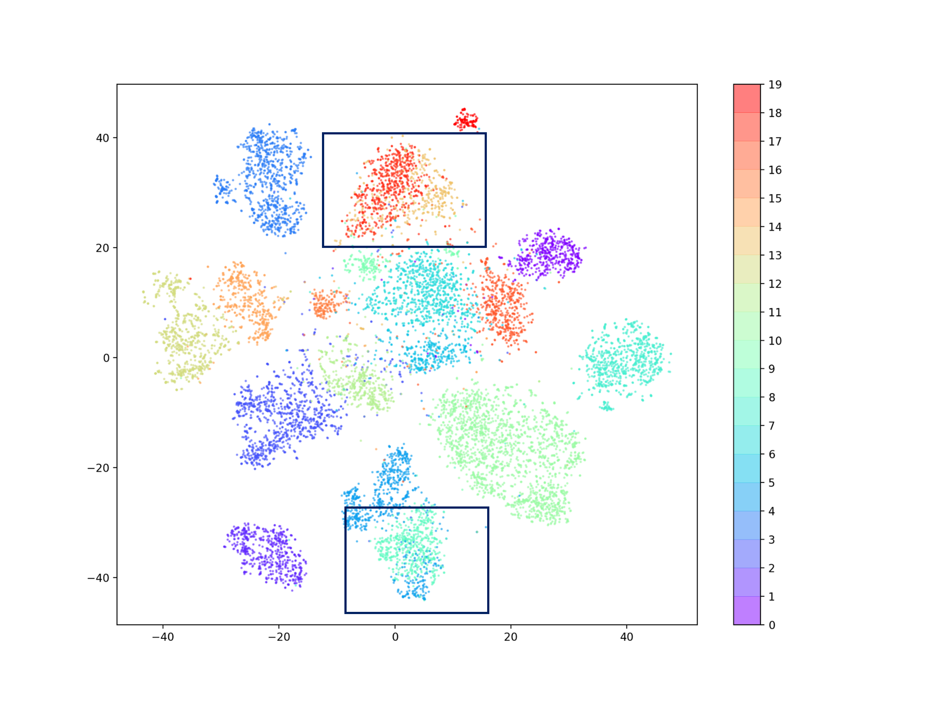
We suspect that the presented pre-training confusion happens in the DIOR case. To validate this, we plot a tSNE embedding of the features of DIOR in Figure LABEL:fig:vit_confusion. One can observe that our pre-trained model confuses between class 13 and class 17 and between class 4 and class 8 (highlighted). That is, the model produces embeddings that are similar for both classes.
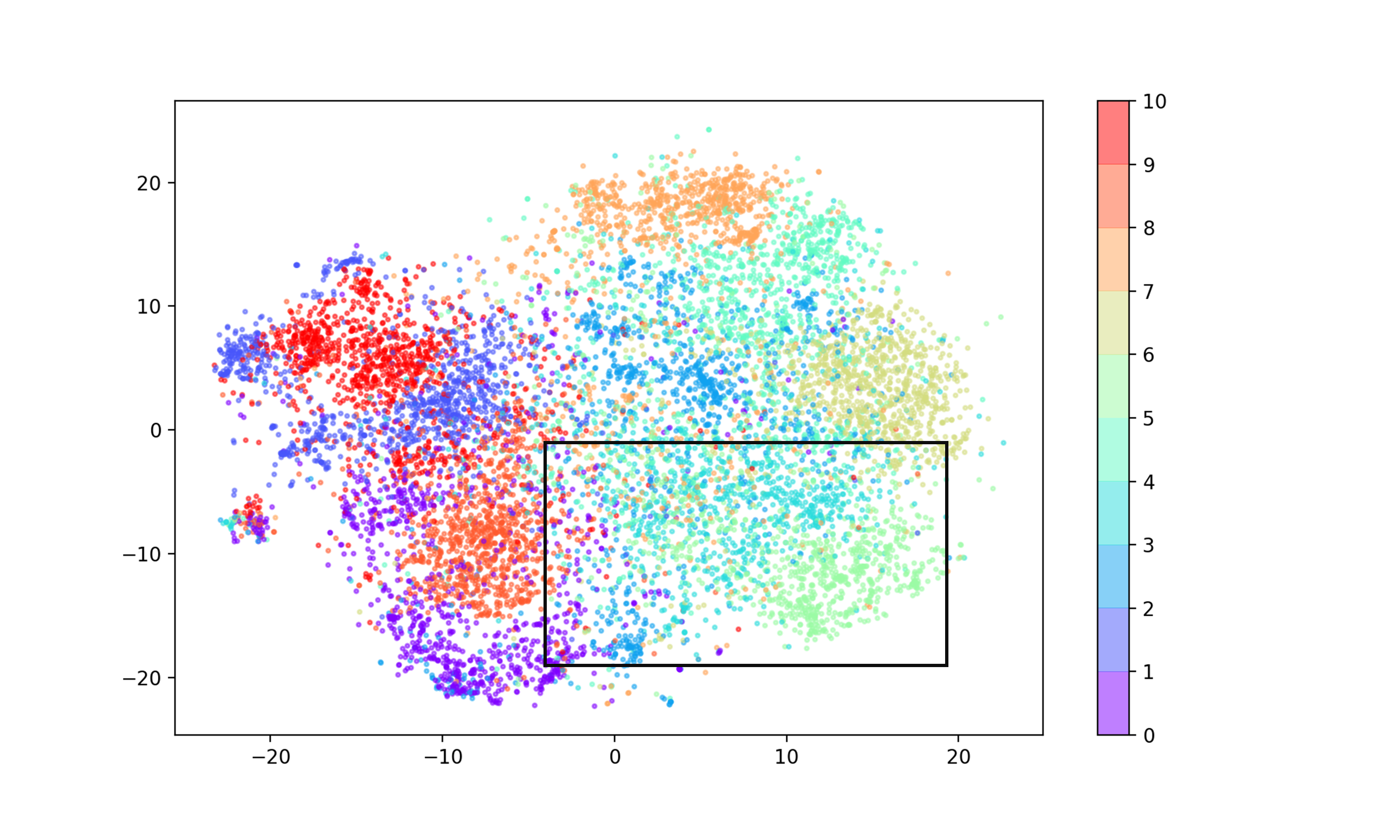
A similar phenomenon occurs with a ResNet architecture as well. This might explain the failure of recently suggested ResNet-based methods on Cifar10 and Cifar100 in the multimodal setting (such as DN2 [5] and PANDA[31]). A tSNE embedding of the pre-trained ResNet features of Cifar10 is plotted in Figure LABEL:fig:resnet_confusion. One can observe that pre-trained ResNet model confuses between class 3 and class 5 (highlighted).
The stress testing of anomaly detection algorithms in the multimodal settings helps to reveal their limitations. We believe that further analyzing anomaly detection in the multimodal setting is an important topic for future research.
5 Conclusions
Transformaly is an anomaly detection algorithm that is based on the Visual Transformer (ViT) architecture. The data is mapped to a pre-trained feature space and a fine-tuned feature space. The normality score of a query point is based on the product of its likelihood in both spaces.
Pre-trained features are obtained by running the samples through a pre-trained ViT. Fine-tuned features are obtained by training a student-network, on normal data only. The discrepancy between student and teacher networks forms the fine-tuned features.
We conduct extensive experiments on multiple datasets and obtain consistently good results, often surpassing the current state of the art.
References
- [1] Chest X-ray (Covid-19 & Pneumonia).
- [2] Intel Image Classification | Kaggle.
- [3] Faruk Ahmed and Aaron Courville. Detecting semantic anomalies. In Proceedings of the AAAI Conference on Artificial Intelligence, volume 34, pages 3154–3162, 2020.
- [4] Gbeminiyi Ajayi. Multi-class Weather Dataset for Image Classification. 1, Sept. 2018. Publisher: Mendeley Data.
- [5] Liron Bergman, Niv Cohen, and Yedid Hoshen. Deep nearest neighbor anomaly detection. arXiv preprint arXiv:2002.10445, 2020.
- [6] Liron Bergman and Yedid Hoshen. Classification-based anomaly detection for general data. In International Conference on Learning Representations (ICLR), 2020.
- [7] Paul Bergmann, Michael Fauser, David Sattlegger, and Carsten Steger. Mvtec ad–a comprehensive real-world dataset for unsupervised anomaly detection. In Proceedings of the IEEE/CVF Conference on Computer Vision and Pattern Recognition, pages 9592–9600, 2019.
- [8] Paul Bergmann, Michael Fauser, David Sattlegger, and Carsten Steger. Uninformed students: Student-teacher anomaly detection with discriminative latent embeddings. In Proceedings of the IEEE/CVF Conference on Computer Vision and Pattern Recognition, pages 4183–4192, 2020.
- [9] Ting Chen, Simon Kornblith, Mohammad Norouzi, and Geoffrey Hinton. A simple framework for contrastive learning of visual representations. In International conference on machine learning, pages 1597–1607. PMLR, 2020.
- [10] Lucas Deecke, Lukas Ruff, Robert A Vandermeulen, and Hakan Bilen. Transfer-based semantic anomaly detection. In International Conference on Machine Learning, pages 2546–2558. PMLR, 2021.
- [11] Lucas Deecke, Robert Vandermeulen, Lukas Ruff, Stephan Mandt, and Marius Kloft. Image anomaly detection with generative adversarial networks. In Joint european conference on machine learning and knowledge discovery in databases, pages 3–17. Springer, 2018.
- [12] Jia Deng, Wei Dong, Richard Socher, Li-Jia Li, Kai Li, and Li Fei-Fei. Imagenet: A large-scale hierarchical image database. In 2009 IEEE conference on computer vision and pattern recognition, pages 248–255. Ieee, 2009.
- [13] Alexey Dosovitskiy, Lucas Beyer, Alexander Kolesnikov, Dirk Weissenborn, Xiaohua Zhai, Thomas Unterthiner, Mostafa Dehghani, Matthias Minderer, Georg Heigold, Sylvain Gelly, Jakob Uszkoreit, and Neil Houlsby. An image is worth 16x16 words: Transformers for image recognition at scale. In 9th International Conference on Learning Representations, ICLR 2021, Virtual Event, Austria, May 3-7, 2021. OpenReview.net, 2021.
- [14] Eleazar Eskin, Andrew Arnold, Michael Prerau, Leonid Portnoy, and Sal Stolfo. A geometric framework for unsupervised anomaly detection. In Applications of data mining in computer security, pages 77–101. Springer, 2002.
- [15] Michael Glodek, Martin Schels, and Friedhelm Schwenker. Ensemble gaussian mixture models for probability density estimation. Computational statistics, 28(1):127–138, 2013.
- [16] Izhak Golan and Ran El-Yaniv. Deep anomaly detection using geometric transformations. In Proceedings of the 32nd International Conference on Neural Information Processing Systems, NIPS’18, page 9781–9791, Red Hook, NY, USA, 2018. Curran Associates Inc.
- [17] Jean-Bastien Grill, Florian Strub, Florent Altché, Corentin Tallec, Pierre H. Richemond, Elena Buchatskaya, Carl Doersch, Bernardo Ávila Pires, Zhaohan Guo, Mohammad Gheshlaghi Azar, Bilal Piot, Koray Kavukcuoglu, Rémi Munos, and Michal Valko. Bootstrap your own latent - A new approach to self-supervised learning. In Hugo Larochelle, Marc’Aurelio Ranzato, Raia Hadsell, Maria-Florina Balcan, and Hsuan-Tien Lin, editors, Advances in Neural Information Processing Systems 33: Annual Conference on Neural Information Processing Systems 2020, NeurIPS 2020, December 6-12, 2020, virtual, 2020.
- [18] Kaiming He, Haoqi Fan, Yuxin Wu, Saining Xie, and Ross Girshick. Momentum contrast for unsupervised visual representation learning. In Proceedings of the IEEE/CVF Conference on Computer Vision and Pattern Recognition, pages 9729–9738, 2020.
- [19] Dan Hendrycks and Kevin Gimpel. A baseline for detecting misclassified and out-of-distribution examples in neural networks. Proceedings of International Conference on Learning Representations, 2017.
- [20] Dan Hendrycks, Xiaoyuan Liu, Eric Wallace, Adam Dziedzic Rishabh Krishnan, and Dawn Song. Pretrained transformers improve out-of-distribution robustness. In Association for Computational Linguistics, 2020.
- [21] Dan Hendrycks, Mantas Mazeika, and Thomas Dietterich. Deep anomaly detection with outlier exposure. Proceedings of the International Conference on Learning Representations, 2019.
- [22] Dan Hendrycks, Mantas Mazeika, Saurav Kadavath, and Dawn Song. Using self-supervised learning can improve model robustness and uncertainty. Advances in Neural Information Processing Systems (NeurIPS), 2019.
- [23] Alex Krizhevsky, Geoffrey Hinton, et al. Learning multiple layers of features from tiny images. 2009.
- [24] Chun-Liang Li, Kihyuk Sohn, Jinsung Yoon, and Tomas Pfister. Cutpaste: Self-supervised learning for anomaly detection and localization. In Proceedings of the IEEE/CVF Conference on Computer Vision and Pattern Recognition, pages 9664–9674, 2021.
- [25] Dan Li, Dacheng Chen, Jonathan Goh, and See-kiong Ng. Anomaly detection with generative adversarial networks for multivariate time series. arXiv preprint arXiv:1809.04758, 2018.
- [26] Shiyu Liang, Yixuan Li, and R. Srikant. Enhancing the reliability of out-of-distribution image detection in neural networks. In 6th International Conference on Learning Representations, ICLR 2018, Vancouver, BC, Canada, April 30 - May 3, 2018, Conference Track Proceedings. OpenReview.net, 2018.
- [27] Luke Melas-Kyriazi. ViT PyTorch, Oct. 2021. original-date: 2020-10-25T18:36:57Z.
- [28] Pankaj Mishra, Riccardo Verk, Daniele Fornasier, Claudio Piciarelli, and Gian Luca Foresti. VT-ADL: A vision transformer network for image anomaly detection and localization. In 30th IEEE/IES International Symposium on Industrial Electronics (ISIE), June 2021.
- [29] Leif E Peterson. K-nearest neighbor. Scholarpedia, 4(2):1883, 2009.
- [30] Jonathan Pirnay and Keng Chai. Inpainting transformer for anomaly detection. arXiv preprint arXiv:2104.13897, 2021.
- [31] Tal Reiss, Niv Cohen, Liron Bergman, and Yedid Hoshen. Panda: Adapting pretrained features for anomaly detection and segmentation. In Proceedings of the IEEE/CVF Conference on Computer Vision and Pattern Recognition, pages 2806–2814, 2021.
- [32] Tal Reiss and Yedid Hoshen. Mean-shifted contrastive loss for anomaly detection. arXiv preprint arXiv:2106.03844, 2021.
- [33] Tal Ridnik, Emanuel Ben-Baruch, Asaf Noy, and Lihi Zelnik-Manor. Imagenet-21k pretraining for the masses. In Thirty-fifth Conference on Neural Information Processing Systems Datasets and Benchmarks Track (Round 1), 2021.
- [34] Lukas Ruff, Robert Vandermeulen, Nico Goernitz, Lucas Deecke, Shoaib Ahmed Siddiqui, Alexander Binder, Emmanuel Müller, and Marius Kloft. Deep one-class classification. In Jennifer Dy and Andreas Krause, editors, Proceedings of the 35th International Conference on Machine Learning, volume 80 of Proceedings of Machine Learning Research, pages 4393–4402. PMLR, 10–15 Jul 2018.
- [35] Mohammadreza Salehi, Ainaz Eftekhar, Niousha Sadjadi, Mohammad Hossein Rohban, and Hamid R Rabiee. Puzzle-ae: Novelty detection in images through solving puzzles. arXiv preprint arXiv:2008.12959, 2020.
- [36] Bernhard Schölkopf, Robert C Williamson, Alexander J Smola, John Shawe-Taylor, John C Platt, et al. Support vector method for novelty detection. In NIPS, volume 12, pages 582–588. Citeseer, 1999.
- [37] shenggan. BCCD Dataset, Oct. 2021. original-date: 2017-12-07T11:54:25Z.
- [38] Kihyuk Sohn, Chun-Liang Li, Jinsung Yoon, Minho Jin, and Tomas Pfister. Learning and evaluating representations for deep one-class classification. In International Conference on Learning Representations, 2021.
- [39] Jihoon Tack, Sangwoo Mo, Jongheon Jeong, and Jinwoo Shin. Csi: Novelty detection via contrastive learning on distributionally shifted instances. In Advances in Neural Information Processing Systems, 2020.
- [40] David MJ Tax and Robert PW Duin. Support vector data description. Machine learning, 54(1):45–66, 2004.
- [41] Sunil Thulasidasan, Sushil Thapa, Sayera Dhaubhadel, Gopinath Chennupati, Tanmoy Bhattacharya, and Jeff Bilmes. A simple and effective baseline for out-of-distribution detection using abstention. 2020.
- [42] Shashanka Venkataramanan, Kuan-Chuan Peng, Rajat Vikram Singh, and Abhijit Mahalanobis. Attention guided anomaly localization in images. In European Conference on Computer Vision, pages 485–503. Springer, 2020.
- [43] Apoorv Vyas, Nataraj Jammalamadaka, Xia Zhu, Dipankar Das, Bharat Kaul, and Theodore L Willke. Out-of-distribution detection using an ensemble of self supervised leave-out classifiers. In Proceedings of the European Conference on Computer Vision (ECCV), pages 550–564, 2018.
- [44] Lin Wang and Kuk-Jin Yoon. Knowledge distillation and student-teacher learning for visual intelligence: A review and new outlooks. IEEE Transactions on Pattern Analysis and Machine Intelligence, 2021.
- [45] Yan Xia, Xudong Cao, Fang Wen, Gang Hua, and Jian Sun. Learning discriminative reconstructions for unsupervised outlier removal. In Proceedings of the IEEE International Conference on Computer Vision, pages 1511–1519, 2015.
- [46] Han Xiao, Kashif Rasul, and Roland Vollgraf. Fashion-mnist: a novel image dataset for benchmarking machine learning algorithms. arXiv preprint arXiv:1708.07747, 2017.
- [47] Zhisheng Xiao, Qing Yan, and Yali Amit. Do we really need to learn representations from in-domain data for outlier detection? arXiv preprint arXiv:2105.09270, 2021.
- [48] Houssam Zenati, Chuan Sheng Foo, Bruno Lecouat, Gaurav Manek, and Vijay Ramaseshan Chandrasekhar. Efficient gan-based anomaly detection. arXiv preprint arXiv:1802.06222, 2018.
- [49] Çağlar Fırat Özgenel. Concrete Crack Images for Classification. 2, July 2019. Publisher: Mendeley Data.
6 Appendix
In this section we will further explain the datasets we used, present the gaussian nuture of the pre-trained features and demonstrate our method’s robustness.
6.1 Datasets Details
CIFAR consists of two well known datasets, Cifar10 and Cifar100, that are used for various tasks including semantic anomaly detection [23]. Each dataset contains color natural images, split into training images and test images. Cifar10 is composed of 10 equal-sized classes, whereas cifar100 has 100 equal-sized fine-grained classes or 20 equal-sized coarse-grained classes. Following the previous papers, we use the coarse-grained classes notation.
Fashion MNIST consists of train samples and examples test samples [46]. Each example is a grayscale image labeled with one of 10 different categories.
Cats Vs Dogs is a dataset of images of cats and dogs. The training set contains images of cats and images of dogs, while the test set contains dog images and cat images. There is either a dog or a cat in every image, appearing in a variety of poses and scenes. Following previous work [5, 31], we split each class to the first images for training and the last 2,500 for testing.
Dior contains aerial images with 19 object categories. Following previous papers [5, 31], we used the bounding boxes provided with the data, and we took objects with at least 120 pixels in each axis as well as only classes with more than 50 images. This preprocessing phase led to 19 classes, with an average training size of 649 images. The sample sizes in each class are not equal, as the lowest sample size in the training set is 116 and the highest is 1890.
Blood Cells [37] contains augmented color images of four different cell types. The training set contains approximately images for each blood cell type, whereas the test set contains approximatly images for each type of blood cell.
Covid19 [1] is a dataset of Chest X-ray images of Covid19, Pneumonia and normal patients.We ignore the Pneumonia patients’ scans and have used just the Covid19 and normal scans. Covid19 patients’ chest X-rays have been divided into images in the training set and images in the test set. The chest X-ray images of normal patients have been divided into images for the training set and images for the test set. Normal patients’ scans are obviously considered normal, while Covid19 patients’ scans are considered anomalous.
View Recognition [2] is an image dataset of natural scenes around the world. This dataset is composed of six different classes such as images of forest and streets. The training set contains approximately images for each class, while the test set contains approximatly images for each class.
Weather Recognition [4] is a multi-class dataset of weather images designed for image classification. There are four types of outdoor weather images in this dataset, including shine and rain. The training set consists of approximately images per class, while the test set contains approximately images per class.
Concrete Crack Classification [49] contains color concrete images with and without cracks. There are images per class in the training set and per class images in the test set. Images of concrete without cracks are considered normal, while images of concrete with cracks are considered anomalous.
6.2 Gaussian nature of data
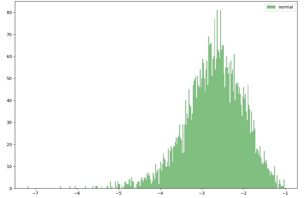
In this section, we presents the fine-tuned feature empirical distribution, that explains why a Gaussian is used to model this data. Figure 5 shows the Teacher-Student fine-tuned features of the last ViT block, using class 0 samples as the normal training set. As one can observe, the fine-tuned features follow a distribution close to Gaussian, which motivate us to use a Gaussian to model the data. We observed similar empirical distributions using different ViT blocks and other normal classes.
6.3 Transformaly Robust Results
To further demonstrate our robust results, we repeated our unimodal experiments three times. In each of the three trials, we calculate the average AUROC score across all possible class choices. Table 8 shows the mean and standard deviation scores of our method, calculated over these three trails. Transformaly achieved similar results, still outperforming other methods on all datasets, except for FMNIST.
| Dataset | CSI | DN2 | PANDA | MSAD | Ours |
| CIFAR10 | 94.3 | 92.5 | 96.2 | 97.2 | 98.34( 0.018) |
| CIFAR100 | 89.6 | 94.1 | 94.1 | 96.4 | 97.60( 0.184) |
| FMNIST | - | 94.5 | 95.6 | 94.21 | 94.37( 0.041) |
| CatsVsDogs | 86.3 | 96.0 | 97.3 | 99.3 | 99.47( 0.037) |
| DIOR | 78.5 | 92.2 | 94.3 | 97.2 | 98.33( 0.177) |