FastGPL: a C++ library for fast evaluation of generalized polylogarithms

Abstract

We present FastGPL, a C++ library for the fast evaluation of generalized polylogarithms which appear in many multi-loop Feynman integrals. We implement the iterative algorithm proposed by Vollinga and Weinzierl in a two-step approach, i.e., we generate concise expressions using an external program and hard-code them into the numeric library. This allows efficient and accurate numeric evaluations of generalized polylogarithms suitable for Monte Carlo integration and event generation. Floating-point arithmetics are carefully taken care of to avoid loss of accuracy. As an application and demonstration, we calculate the two-loop corrections for Higgs boson production in the vector boson fusion channel at electron-positron colliders. FastGPL is expected to be useful for event generators at the next-to-next-to-leading order accuracy.

PROGRAM SUMMARY

Program Title: FastGPL
Developer’s repository link: https://github.com/llyang/FastGPL
Code Ocean capsule: (to be added by Technical Editor)
Licensing provisions (please choose one): LGPL
Programming language: C++
Supplementary material:
Journal reference of previous version:
Does the new version supersede the previous version?:
Reasons for the new version:
Summary of revisions:
Nature of problem: Fast numerical evaluation of generalized polylogarithms [1].
Solution method: A two-step implementation of the algorithm of [2], where hard-coded expressions are generated by an external program.
Additional comments including restrictions and unusual features: Currently limited to GPLs up to weight 4.

1 Introduction

The generalized polylogarithms (GPLs, also called multiple polylogarithms, i.e., MPLs) [Goncharov:1998kja] appear in many cutting-edge calculations of Feynman integrals and scattering amplitudes. In order to use these amplitudes to compute differential cross sections or to generate Monte Carlo event samples, it is highly desirable to obtain numeric values of GPLs as efficient as possible. A general algorithm for the numeric evaluation of GPLs has be proposed in [Vollinga:2004sn]. An implementation of this algorithm has been built into the symbolic computation library GiNaC [Bauer:2000cp, Vollinga:2005pk]. However, by default GiNaC is not suitable for fast numeric calculations since it is designed to work best with numbers of unlimited precision (as implemented in the CLN library).

A reimplementation of the algorithm using Fortran has appeared recently under the name handyG [Naterop:2019xaf]. It is designed for the purpose of fast numeric evaluation suitable for Monte Carlo event generations. It has since then been widely used in multi-loop calculations as a fast alternative to GiNaC. However, during our usage of it, we found some drawbacks of the program which motivated us to write our own private implementation of the same algorithm. This gradually grows up into the library FastGPL presented in this work.

The main drawbacks of handyG that we found can be summarized in the following: 1) The algorithm of [Vollinga:2004sn] is an iterative one. If one naively follows the iterative approach, there can be situations where some functions are computed many times for the evaluation of one particular GPL. This greatly slows down the evaluation for such GPLs. For example, the average evaluation time for a single weight-4 GPL on a modern computer is about $10^{-4}$ seconds. However, as we will see in Section 3, the evaluation time of certain weight-4 GPLs can be as long as $\mathcal{O}(1)$ second. 2) The series representation of GPLs may sometimes lead to terms exceeding the maximal value that can be hold by a double-precision floating-point number. When this happens, handyG simply truncates the series, which leads to a loss of accuracy. This problem can of course be circumvented by using the quad-precision version of handyG. This however slows down the computation much more than necessary, if one only needs the final result in double-precision. 3) Partly due to the iterative nature of the algorithm, floating-point cancellations among different contributions often happen. In certain cases this leads to non-negligible losses of accuracy without careful treatment.

The aim of FastGPL is avoid the above problems as much as possible in a floating-point implementation of the algorithm of [Vollinga:2004sn], while providing the overall efficiency and accuracy similar to handyG. This paper is organized as follows. In Section 2, we briefly introduce the notations and some important properties of GPLs. In Section 3, we describe the program FastGPL, and provide some validations and benchmarks. In Section 4 we discuss a working application in the two-loop corrections for the $e^{+}e^{-}\to\nu\mathrm{bar}{\nu}H$ scattering process. Finally we conclude in Section LABEL:sec:summary. In the Appendix, we describe how to obtain, install and use FastGPL.

2 Notations and properties of GPLs

In this section, we setup our notations and introduce some important properties of GPLs which will be used in their numeric computation. For a more comprehensive review, we refer the interested readers to Refs. [Duhr:2014woa]. GPLs are complex-valued functions depending on a sequence of complex parameters $a_{1},\ldots,a_{n}$ (we will often collectively refer to this sequence as $\bm{a}$) as well as a complex argument $z$. A GPL can be defined recursively as

$$G(\bm{a};z)=G(a_{1},\ldots,a_{n};z) \equiv\int_{0}^{z}\frac{dt_{1}}{t_{1}-a_{1}}G(a_{2},\ldots,a_{n};t_{1})\,.$$ (1)

with the initial kernels

$$\quad G(;z)\equiv 1\,,\quad G(\underbrace{0,\ldots,0}_{n};z)\equiv G(\bm{0}_{n};z)\equiv\frac{\log^{n}z}{n!}\,,$$ (2)

where $\bm{0}_{n}$ denotes a sequence of $n$ zeros. We will call the parameters $a_{i}$’s as the indices of the GPL. The number of indices is called the weight of the GPL.

The GPLs satisfy a set of relations called the shuffle algebra. The product of a weight-$n$ GPL and a weight-$m$ GPL can be expressed as the sum of a number of weight-$(n+m)$ GPLs as following:

$$G(\bm{a};z)\,G(\bm{b};z)=\sum_{\bm{c}\in\bm{a}\shuffle\bm{b}}G(\bm{c};z)\,,$$ (3)

where $\bm{a}=\{a_{1},\ldots,a_{n}\}$, $\bm{b}=\{b_{1},\ldots,b_{m}\}$, and $\bm{a}\shuffle\bm{b}$ denotes the shuffle product of the two sequences $\bm{a}$ and $\bm{b}$. Briefly speaking, an element in the shuffle product is a rearrangement of the entries in $\bm{a}$ and $\bm{b}$, such that the relative orders within $\bm{a}$ and $\bm{b}$ are preserved. As an example, considering the case $n=m=2$, we have

$$\bm{a}\shuffle\bm{b}=\big{\{}\{a_{1},a_{2},b_{1},b_{2}\}\,,\{a_{1},b_{1},a_{2},b_{2}\}\,,\{a_{1},b_{1},b_{2},a_{2}\}\,,$$

$$\{b_{1},a_{1},a_{2},b_{2}\}\,,\{b_{1},a_{1},b_{2},a_{2}\}\,,\{b_{1},b_{2},a_{1},a_{2}\}\big{\}}\,.$$ (4)

GPLs with the last index $a_{n}=0$ are logarithmic divergent when $z\to 0$, which prevents a series representation in that region. The shuffle algebra can be used to remove these “trailing zeros” and to extract the divergences. For example, we have

$$G(a_{1},a_{2},0;z)=\log(z)\,G(a_{1},a_{2};z)-G(0,a_{1},a_{2};z)-G(a_{1},0,a_{2};z)\,.$$ (5)

While this step can be taken care of numerically, it is strongly suggested to perform it analytically before feeding the expression into a numeric program. This avoids the unnecessary overhead in the numeric evaluation, and also allows one to transform the argument $z$ of the remaining GPLs to a non-negative real number (to be discussed later).

The evaluation of GPLs without trailing zeros boils down to computing the partial sum of their series representation. For that purpose, we first introduce the compressed notation of GPLs:

$$G_{m_{1},\ldots,m_{k}}(a_{1},\ldots,a_{k};z)\equiv G(\bm{0}_{m_{1}-1},a_{1},\ldots,\bm{0}_{m_{k}-1},a_{k};z)\,,$$ (6)

where $a_{1},\ldots,a_{k}$ are non-zero. Such a GPL can be expanded as

$$G_{m_{1},\ldots,m_{k}}(a_{1},\ldots,a_{k};z)=(-1)^{k}\sum_{i_{1}>\cdots>i_{k}>0}\frac{\left(\frac{z}{a_{1}}\right)^{i_{1}}}{i_{1}^{m_{1}}}\frac{\left(\frac{a_{1}}{a_{2}}\right)^{i_{2}}}{i_{2}^{m_{2}}}\cdots\frac{\left(\frac{a_{k-1}}{a_{k}}\right)^{i_{k}}}{i_{k}^{m_{k}}}\,,$$ (7)

which converges under the conditions $|z|\leq|a_{i}|,(i=1,\ldots,k)$, and if $m_{1}=1$, one requires in addition $z\neq a_{1}$ (otherwise the GPL is logarithmic divergent). If these conditions are satisfied, we call the corresponding GPL as a “convergent” GPL. In a numeric implementation of Eq. (7), one truncates the infinite series such that the remaining terms are negligible for a chosen accuracy. Already at this point, one can imagine that, for certain values of the indices and the argument, the powers of ratios in Eq. (7) can exceed the maximal value allowed in a given floating-point representation. Whether this may happen in practice is something we’ll discuss in the next section.

It is easy to realize that not all GPLs are convergent in the sense of Eq. (7). The main idea of the algorithm in [Vollinga:2004sn] is to use the integral representation and the properties of GPLs to transform a given non-convergent GPL to a linear combination of convergence ones. We are not going to describe the algorithm in detail but refer the interested readers to [Vollinga:2004sn, Naterop:2019xaf]. It suffices to mention that, one may encounter the same (convergent or non-convergent) GPL many times in this multi-step transformation, which then needs to be evaluated many times if the algorithm is implemented recursively.

A GPL without trailing zeros satisfies another useful relation:

$$G(a_{1},\ldots,a_{m};z)=G(\lambda a_{1},\ldots,\lambda a_{m};\lambda z)\,,$$ (8)

for any non-zero complex number $\lambda$. This property can be used to convert the argument $z$ of GPLs to be a non-negative real number. This allows the program to easily decide which side of a branch cut to take according to the signs of the imaginary parts of the indices. This is important since quite often the imaginary parts of the parameters are infinitesimal ones coming from the Feynman $+i\epsilon$ prescription. Setting a small imaginary part instead of an infinitesimal one is sometimes unacceptable in a numeric computation. Therefore, in FastGPL we require the input argument $z$ to be a non-negative real numbers, and allow the users to indicate the signs of the infinitesimal imaginary parts with an extra set of input parameters. This convention is the same as GiNaC.

3 The program library FastGPL

3.1 Implementation

The implementation of FastGPL is a two-step process. An in-house program in Mathematica is built up to perform the transformation from non-convergent GPLs to convergent ones. Note that the transformation is different for different relative sizes of the indices $\{a_{i}\}$, and the program needs to generate an expression for each individual case. The resulting expressions consisting of convergent GPLs and a few lower-weight non-convergent ones are then converted to C++. Abbreviations are introduced at this step such that each function in the expression for a given GPL is computed only once. The Mathematica code is not fully automatic at the moment, and therefore only GPLs up to weight-4 have been currently implemented.

Avoiding the repeated evaluations of the same GPLs can lead to significant performance gain in certain cases. Take

$$\mathtt{G(1.0025,0.989,0.45,0.89+0.24i;1)}$$

as an example. In an iterative implementation of the algorithm, various weight-3 and weight-4 GPLs need to be recursively evaluated for $\mathcal{O}(500000)$ times. This significantly slows down the computation, and it takes handyG about 2 seconds to evaluate the above GPL. On the other hand, the evaluation time of FastGPL is less than 0.01 seconds. The non-iterative implementation of FastGPL also reduces the accuracy losses due to floating-point arithmetics, and the resulting precision is usually better or at least comparative. Here and in the following, all benchmarks are performed using a single core of an Intel Xeon E5-1680v3 CPU with the gcc 9.4 compiler under Ubuntu Linux 18.04.

After transforming to convergent GPLs, they can then be computed using the series representation (7). While this is a trivial exercise for a program using unlimited precision numbers (such as GiNaC), it is a bit challenging for a program using floating point numbers. The problem is that although the terms in Eq. (7) gradually become smaller order-by-order, some of the powers $(a_{j-1}/a_{j})^{i_{j}}$ may become very large at high orders. They could exceed the maximal value that can be stored in a floating-point format (which is about $10^{308}$ for double-precision). One may truncate the series before that happens, which however leads to a loss of accuracy. One may also use a floating-point format with more bits which can represent numbers in a bigger range. Such an option is provided in handyG, where 128-bit quad-precision numbers can be used throughout. This however significantly slows down the computation, which is certainly not desirable if one only needs the final results in double-precision. FastGPL approaches this problem slightly differently: it switches to a higher-precision format (long double at the moment, which however is compiler-dependent) only when necessary, i.e., when it detects the possibility of overflow.

	$g_{1}\times 10^{5}$	$g_{2}\times 10^{5}$
GiNaC	$\mathtt{3.6870217689293}$ $\mathtt{-7.5295211195637i}$	$\mathtt{1.01839797324439}$ $\mathtt{-1.50327528421384i}$
FastGPL	$\mathtt{3.6870217689292}$ $\mathtt{-7.5295211195637i}$	$\mathtt{1.01839797324439}$ $\mathtt{-1.50327528421384i}$
handyG	$\mathtt{3.6874023785452}$ $\mathtt{-7.5284903971195i}$	$\mathtt{1.01819546357542}$ $\mathtt{-1.50329421576427i}$

Table 1: A demonstration of accuracy-loss due to floating-point overflow occurred in handyG but not in FastGPL.

The above approach has been tested at millions of randomly sampled points, and also in realistic applications. No truncation of the series is observed. As a demonstration, we show in Table 1 the results for the following two GPLs:

$$g_{1} =\mathtt{G(-223.7-576.0i,-0.29-0.74i,-0.29-0.74i,0.26+0.67i;1)}\,,$$

$$g_{2} =\mathtt{G(0.24+0.61i,-0.21-0.55i,0,-4735.0-12190.9i;1)}\,.$$

It can be seen that the results of FastGPL agree perfectly with those of GiNaC. On the other hand, the results of handyG deviate relatively by as much as $10^{-4}$. Note that the above GPLs appear in the calculation of a two-loop scattering amplitude to be presented later. Hence it is not just an academic study but have practical consequences.

3.2 Benchmarks

We have performed a thorough test of FastGPL at weights 1, 2, 3 and 4 with randomly generated parameters. The relative precision of weight-4 GPLs is typically at the level of $10^{-13}$ or better. The lower weight GPLs are of course more accurate. We believe that this is enough for most phenomenological applications.

FastGPL is built with efficiency in mind. In the following we show some benchmarks of it in the computations of weight-4 GPLs. The number of iterations needed for a GPL depends crucially on the absolute values of the non-zero indices $\{a_{i}\}$ compared to the argument $x$. Hence we classify weight-4 GPLs into several categories accordingly, and investigate the typical time required for their evaluations. We will use lowercase letters to label “small” indices, i.e., $|a|<|x|$; and use uppercase letters to label “big” indices, i.e., $|A|\geq|x|$. For example, $0abC$ denotes a category of weight-4 GPLs with one zero-index, two small indices and a big index. Note that the order of the indices is irrelevant in this classification.

	$t_{\text{f}}$ (s)	$t_{\text{h}}$ (s)	$t_{\text{h}}/t_{\text{f}}$
$\mathtt{G(1.0025,0.989,0.45,0.89+0.24i;1)}$	$0.006$	$2.2$	$\sim 400$
$\mathtt{G(0.998,1.0545+0.127i,0.91+0.25i,-0.226;1)}$	$0.004$	$1.5$	$\sim 400$
$\mathtt{G(-1.04,-0.97,0.25,-0.84+0.45i;1)}$	$0.004$	$1.1$	$\sim 300$

Table 2: Average evaluation times of several GPLs which require many iterations.

	$0aBC$	$0abC$	$0abc$	$00aB$	$00ab$
$t_{\text{f}}$ (ms)	$0.22$	$0.25$	$0.20$	$0.08$	$0.05$
$t_{\text{h}}$ (ms)	$3.1$	$5.8$	$4.5$	$1.3$	$0.80$
$t_{\text{h}}/t_{\text{f}}$	$\sim 14$	$\sim 23$	$\sim 23$	$\sim 17$	$\sim 16$

	$ABCD$	$abCD$	$abcD$	$abcd$
$t_{\text{f}}$ (ms)	$0.22$	$0.47$	$0.50$	$0.42$
$t_{\text{h}}$ (ms)	$1.7$	$7.4$	$11.0$	$9.1$
$t_{\text{h}}/t_{\text{f}}$	$\sim 7.5$	$\sim 16$	$\sim 22$	$\sim 22$

Table 3: Average evaluation times of a few categories of weight-4 GPLs.

In Table 2, we first show several examples of GPLs that require many iterations in the algorithm. The average evaluation times using FastGPL and handyG are denoted as $t_{f}$ and $t_{h}$, respectively. Apparently these are cases where FastGPL mostly benefits from the preprocessing of the iterative algorithm, and the performance gain is quite impressive. This of course does not represent the generic behaviors of the two programs. In Table 3 we show the average evaluation times of a few categories of weight-4 GPLs, where the indices are randomly sampled within each category. One can see that FastGPL is typically faster by $\sim 20$ times in these situations. In the next section, we apply our program to a realistic calculation of a Higgs production process, to demonstrate its efficiency in practice.

4 Application to $e^{+}e^{-}\to\nu_{e}\mathrm{bar}{\nu}_{e}W^{*}W^{*}\to\nu_{e}\mathrm{bar}{\nu}_{e}H$

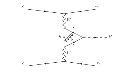
Figure 1: A typical Feynman diagram contributing to the mixed QCD-EW corrections for the Higgs production process via $W$ boson fusion.

Vector boson fusion is one of the dominant Higgs production channels at a future electron-positron collider as a Higgs factory. The expected high experimental precision demands improvements on theoretical calculations for this process. The leading order (LO) and next-to-leading order (NLO) electroweak (EW) corrections for the total and differential cross sections are available in [Altarelli:1987ue, Kilian:1995tr, Belanger:2002me, Denner:2003yg, Denner:2003iy, Denner:2004jy]. Here, we add to those results the next-to-next-to-leading order (NNLO) mixed QCD-EW corrections at order $\alpha\alpha_{s}$. A typical Feynman diagram at this order is shown in Fig. 1.

In our calculation we neglect masses of all light fermions except that of the top quark. We generate the two-loop amplitude using FeynArts [Hahn:2000kx], and manipulate the resulting expressions using Mathematica. The scalar integrals are reduced to a set of master integrals using FIRE6 [Smirnov:2019qkx] and LiteRed [Lee:2013mka]. The expressions for all the master integrals in terms of GPLs can be found in [DiVita:2017xlr, Ma:2021cxg]. We renormalize the fields and the masses in the on-shell scheme, while the fine structure constant $\alpha$ is defined in the $G_{\mu}$ scheme:

$$\alpha_{G_{\mu}}=\frac{\sqrt{2}}{\pi}G_{\mu}m_{W}^{2}\left(1-\frac{m_{W}^{2}}{m_{Z}^{2}}\right).$$ (9)

The standard model parameters are chosen as [ParticleDataGroup:2020ssz]: $m_{t}=$172.76\text{\,}\mathrm{GeV}$$, $m_{H}=$125.1\text{\,}\mathrm{GeV}$$, $m_{Z}=$91.1876\text{\,}\mathrm{GeV}$$, $m_{W}=$80.379\text{\,}\mathrm{GeV}$$, $\alpha_{s}(m_{Z})=0.1179$ and $G_{\mu}=$$.Thedefaultrenormalizationscalefor$α_s$ischosenasthecenter-of-massenergy$μ=s$.\text{Table 4Table 4tableTabletablesTables4Table 4s (GeV)σLO (fb)δσNNLO (fb)tf (h)th (h)th/tf2507.880.0100.458.60∼1935030.60.0400.519.02∼1850074.80.1010.529.24∼184Resultsforth}$

References

- [1] A. B. Goncharov, Multiple polylogarithms, cyclotomy and modular complexes, Math. Res. Lett. 5 (1998) 497 [1105.2076].
- [2] J. Vollinga and S. Weinzierl, Numerical evaluation of multiple polylogarithms, Comput. Phys. Commun. 167 (2005) 177 [hep-ph/0410259].