ESAFE: Enterprise Security and Forensics at Scale

Abstract

Securing enterprise networks presents challenges in terms of both their size and distributed structure. Data required to detect and characterize malicious activities may be diffused and may be located across network and endpoint devices. Further, cyber-relevant data routinely exceeds total available storage, bandwidth, and analysis capability, often by several orders of magnitude. Real-time detection of threats within or across very large enterprise networks is not simply an issue of scale, but also a challenge due to the variable nature of malicious activities and their presentations. The system seeks to develop a hierarchy of cyber reasoning layers to detect malicious behavior, characterize novel attack vectors and present an analyst with a contextualized human-readable output from a series of machine learning models. We developed machine learning algorithms for scalable throughput and improved recall for our Multi-Resolution Joint Optimization for Enterprise Security and Forensics (ESAFE) solution. This Paper will provide an overview of ESAFE’s Machine Learning Modules, Attack Ontologies, and Automated Smart Alert generation which provide multi-layer reasoning over cross-correlated sensors for analyst consumption.

1 Introduction

While current-day enterprise networks are becoming increasingly larger and more complex, cyber-adversaries are also becoming increasingly more sophisticated with an ever enlarging repertoire of attack tools and techniques. New attack vectors are fueled by vulnerabilities of various kinds in increasingly more complex software and made more dangerous with increasing connectivity and scale of enterprise networks. Cyber-security solutions are therefore increasingly crucial and challenging. Robust solutions requires a multi-layer approach that brings together multiple sensors from a variety of vantage points (e.g., network logs, kernel and application logs, etc.) and performs robust automated threat detection from these sensor feeds. Key requirements for a robust cyber-security solution include:

• Threat detection at scale: With current-day enterprise network sizes, the various sensor logs discussed above are truly massive in volume. To be able to process data in near-real-time, an effective threat detection system must be able to scale to very large data volumes.

• Support for multiple types of sensor data: The various sensors discussed above provide data with very different types of semantics, different time scales, and different structures of numerical and categorical data. An effective threat detection system must be able to scale to different types of sensor data using a coherent unified algorithmic core.

• High accuracy, precision, and recall: Due to the massive data volumes, very high accuracy is crucial for threat detection systems to be effective. False positives (i.e., spuriously declaring threats) are undesirable since any such spurious threat detection would need to be processed/triaged in some way (e.g., by a human operator) and even a low percentage of false positives can quickly overwhelm such a processing/triaging component. When confronted with the possibility of a significant number of false positives, a human operator would, for example, start ignoring the threat detections by the system, thereby making the detection system ineffective.

• Human-understandability of underlying logic/reasons for threat detections: To be able to interpret threat detections and determine possible responses, a human analyst requires a human-comprehensible context for the threat detections and the reasons for why a particular set of data points (e.g., network log entries) were considered a threat. Hence, to be truly effective, an automated threat detection system must be able to provide a human-interpretable identification of the particular fields/features that triggered a threat detection and the decision logic based on these identified fields/features that informed the alert.

To address the challenges highlighted above, we propose Multi-Resolution Joint Optimization for Enterprise Security and Forensics (ESAFE), an integrated framework that brings together multiple complementary ingredients to achieve a robust, scalable, and high-accuracy cyber-security solution:

• To leverage the understanding of signatures of “localized” elemental events to enable detection of novel attacks, ESAFE’s operation is defined in terms of sequences/clusters of elemental labels. Each elemental label is indicative of specific events or behaviors (e.g., failed logons, port scans) and sequences/clusters of such labels are defined as indicative of larger-scale malicious/anomalous behavior.

• For efficient at-scale classification of network/host-based data for detection of elemental labels, a deep neural network (DNN) based methodology is applied based on the Gated Mixture of Experts (GME) architecture. This architecture is scalable to a wide variety of data schemas and can operate at scale to fuse data from multiple sources while automatically picking the specific data source that is most informative for each type of label being considered in multi-label classification.

• To extract a human-understandable context for event classifications and threat detections, a probabilistic parameterized Metric Temporal Logic (ppMTL) based approach is applied, which identifies the specific combinations of features from the sensor data that informed each specific threat detection. The ppMTL component identifies which features are relevant for threat detection and a human-readable representation of the decision logic in terms of these features (as a set of linear inequalities among these identified features).

This paper is organized as follows. The methodology for generation of elemental labels and clusters thereof is discussed in Section 2. The machine learning methodologies based on GME and ppMTL approaches outlined above are described in Section 3. The overall system architecture is discussed in Section 4. The lessons learned are summarized in Section 5. The open challenges and future work are discussed in Section 6.

2 Labeling Methodology

The critical first step in the application of supervised machine learning with respect to the cyber security domain, in particular to the task of finding unknown intrusions via log data, is labeling the data. This presents several nontrivial challenges including: highly unbalanced dataset, intrinsic difficulty in defining what constitutes a network intrusion (which is still an open problem), and labeling “normal” data given the high noise floor in network traffic. Prior research (Sommer and Paxson Sommer and Paxson (2010)) describes the difficulty in observing a sufficient amount of network traffic for enabling classification to have adequate accuracy.

Our first approach was to generalize the current best practice of known signatures and heuristics rules. In generalizing the current rule base, we gained the ability to detect similar behavior at the expense of incurred nominal higher false positive rate for individual rules. Our intention was that secondary reasoning over the initial labeling of the data would consider multiple data sources over a given finite window of time, thus forming identification of a threat vector. This enabled us to summarize for a given system which of our rules fired during a given time window. While this is a minor advancement in the current state of the art in terms of a condensed representation of current generalized rules, it does not address discovering unknown/unseen attacks. Since the rules are directly based on current Security Operations Center (SOC) rules, it bridges the semantic gap as defined by Sommer and Paxson (Sommer and Paxson (2010)) to the current state of practice. They define the semantic gap as effort needed to transfer results into actionable reports for the network operator. Another issue with this approach is scaling: the rate at which new rules can be written can only match current industry standards and these limitations lead us to consider a constructive approach.

Our following approach for labeling data was to deconstruct attack tactics techniques procedures (TTPs) to network artifacts and further deconstruct network artifacts to elemental labels on particular logs. This allowed ESAFE to construct elemental labels from known attacks and form clusters of elemental labels to infer particular TTPs. Below, we discuss two approaches for constructing elemental labels and clusters. In combination, these clusters provide five distinct benefits.

1. Shifts in TTPs from attackers will continue to trigger most of the elemental labels since attackers often evolve their techniques.

2. Unknown/unseen TTPs can be discovered as hybrids of current known TTPs through identification of appropriate composite clusters.

3. Elemental labels are less likely to have legacy issues as they cover a dynamic behavior observed in a log rather than hard-coded rules. As an example of a legacy issue, proxy rules that block a particular domain “www[dot]mal[dot]com” will not fire once the attacker changes the domain.

4. Logs can be studied and elemental rules can be written to ensure coverage prior to having seen evidence of their use by any TTP.

5. Adding a single elemental label can inform many other clusters. This provides a non-linear way to scale the production of clusters which can be detected.

2.1 Data Driven Elemental Labels

Our bottom up approach was to analyze individual logs in order to create data driven elemental building blocks. We created elemental rules for: single rows of data, multiple fixed length rows, and rolling time windows. An example of an elemental rolling time window rule is given by the label “Abandoned Logon Attempt”, wherein the corresponding rule looks for two failed attempted logons and the absence of a successful logon within a given window. Taken in isolation, this elemental feature is not necessarily indicative of an attack and is strictly informative when taken as part of a cluster comprising a network artifact. This elemental feature could be, for example, simply an occurrence of a single user not remembering their password and stopping short of locking their account, supporting evidence of a brute force attack on the network, or many other possibilities. An example of a single row event would be a Windows Event Log ID [4719, 4715, 4812, or 4885] indicating that there was a change in the system audit policy; again, we see an elemental feature describing what is happening, but which by itself does not indicate an attack. Some elemental features, ”anomalous request type cipher for server”, are derived directly from statistical studies of the data. This rule fires for a given server IP if the (version, cipher) pair is anomalous.

2.2 Data Driven Clusters

Our bottom up approach to clustering, taking elemental features and reconstructing network artifacts, was to simply find all labels for a given IP and create a weighted threat vector based on number and severity of elemental features. We then sorted this list and designated the top N nodes as starting points. From our starting points, we map out interactions (IP connections) to all other nodes from our candidate node and repeat the ranking process and follow the next top second degree N nodes. We repeated this process for a max depth of three hops. This was a manual process, which could be automated. The greater concern here is interpreting the cluster with respect to the semantic gap.

Data Driven Elemental Labels (DDEL) provides a method for labeling cyber data without the expectation or knowledge of TTPs. This technique is critical to answering the question: how do we find unknown intrusions via log data? However, the Data Driven Cluster is difficult and in some cases impossible to interpret by the cyber analyst. Exclusively clustering DDEL did not decrease the semantic gap. This motivated the approach to ontological clustering described below.

2.3 Attack Ontology Cluster

Our top down approach is to label known clusters by constructing elemental labels with the available supporting data of known artifacts. Let us indulge in the medical analogy of symptoms and diagnoses. The top down approach utilizes predefined attack types (illnesses) for which elemental labels (symptoms) would eventually through the series of algorithms, described in the following sections, have the ability to be aggregated to support known suspicious activity. For example, given a cough, sore throat, and fever, an inference of the flu would be an actionable assessment of the symptoms. This methodology can then easily be extended to clusters or named attacks (illnesses) which are modified in small ways to attempt to avoid detection. A modified cluster would be considered highly suspicious if it contained many elemental indicators to a known attack cluster and exhibited slight modifications. Also, a hybrid of two known techniques would be detected as one new cluster with components of two partial clusters and considered suspicious. Attack ontology elemental labels create an extensible foundation for detecting named attacks. The semantic gap is bridged by domain knowledge in this approach with the limitation that highly novel attacks, clusters of labels with few or no elemental labels in known clusters, will be missed.

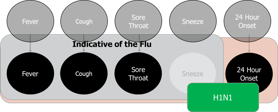
Figure 1: Analogy To Virus Indicators

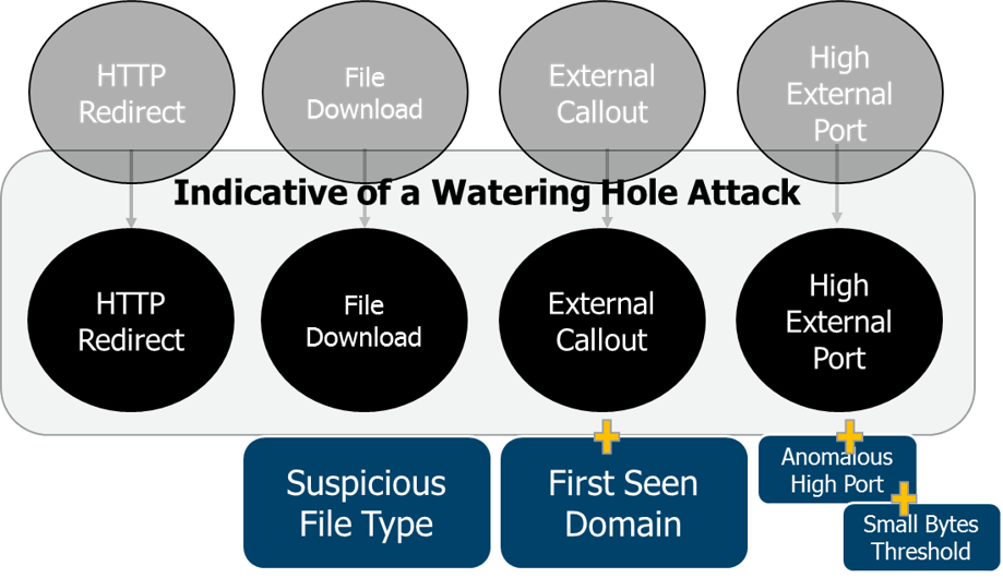
Figure 2: Cluster Ontology

2.4 Attack Ontology Elemental Labels

Once a class of malicious behavior to search for has been identified, the log artifacts that such a behavior would leave behind need to be identified and elemental labels of the smallest atomic units would need to be defined. For example, a network connection, a file modification log entry, or a JA3 hash are all Attack Ontology Elemental Labels (AOEL). In our experiments, we attempted to identify 3-5 AOEL in at least two different data types for each class of malicious behavior we were hunting for. Although we were able to demonstrate some success with this approach, we recognize the following open problems; determining the optimal number of AOEL per cluster, maximizing the abstraction of the attack ontology ensuring cluster labels have the correct overlap, and ensuring that AOEL have coverage of all possible TTP artifacts for a given label.

Figure 3: Attack Ontology Clustering

2.5 Balanced Constructive Labeling Method

In order to discover new unknown attacks and TTPs and bridge the semantic gap, there is no single one best labeling strategy and we need a moderated approach where we have enough AOEL rules to have clusters which are explainable to the user and enough DDEL rules able to find new attacks.

3 Replacing Database Heuristics with Machine Learning

In order to scale to large volumes of data and future perturbations of attacks, there must exist a methodology to appropriately label or enrich the data early on in the reasoning system. The elemental feature enrichments come in a variety of complexities as mentioned in Section 2. Machine Learning classifiers vary in their use cases for certain types of classification, however, in our Cyber Reasoning System, we require partly feature detection and partly feature generation (multilabel classes). While such a machine learning classification can be addressed using a Convolutional Neural Network (CNN), training a vanilla CNN on all concatenated data types for all potential label classes will not work well for networks missing a sensor or experiencing sensor failure. As well, not all labels are of the same complexity, meaning classifier training on labels consisting of single feature single value is different than training for a multiple feature multiple value threshold. In order to enrich the alert feeds coming from commercial and proprietary systems, we apply a Gated Mixture of Experts (GME) architecture. The GME architecture below solves the scale and missing inputs issues while allowing a probabilistic model to operate on the input data. This in itself is fundamental to scalability of finding novel attacks or small perturbations on known attacks. Since labels (enrichments) are not hard coded, the decision boundary hyperplane is in a way fuzzing the rule set. Labels involving strings can allow for string fuzzing, thresholds such as number of bytes can be learned and dynamic in nature from new input data, and series of nested AND/OR statements in traditional named attacks can be reasoned or learned later down the system processing pipeline via their elemental enrichments. To provide a human-understandable explanation of the classifications and resulting threat detections, we apply a probabilistic parameterized Metric Temporal Logic (ppMTL) based approach. The ppMTL based component generates human-readable annotations that identify the specific features in the input data that informed a particular classification and the particular decision logic in terms of these identified features (as a set of linear inequalities). To facilitate human-understandability of the generated explanations, a crucial part of the ppMTL approach is construction of spatio-temporal aggregations of input data (e.g., network logs) from the viewpoints of individual IP addresses in the network. These spatio-temporal aggregations are constructed using a dynamic graph methodology. The GME and ppMTL components in ESAFE are described in Sections 3.1 and 3.2, respectively.

3.1 Gated Mixture of Experts

Crucial challenges in the development of a machine learning based classifier for the cyber-security problem addressed by ESAFE include: scalability to massive amounts of data (e.g., training and running inference over terabytes of data), requirement for near-real-time performance (since robust cyber-security requires rapid visibility into on-going attacks; also, slower than real-time throughput will result in growing back-logs), robustness to varying availabilities of individual sensor feeds (e.g., absence of some sensors on some networks or for some time periods) and ability to generate classification outputs with only partially observable or missing inputs. The GME’s main function in the ESAFE pipeline is multilabel classification of event indicators (labels discussed in Section 2) for each row of data fed in as part of a window of $N$ rows of data (where $N$ is a window size parameter, e.g., $N=100$ is the default setting in our experiments). The high level architecture is shown in Figs. 4 and 5. The pipeline of data consists of fetching a window across sensors, data formatting, and inference. The data from each sensor is processed by a specialized network (an expert) for that particular sensor data and the outputs of the different experts are combined using a gating mechanism.

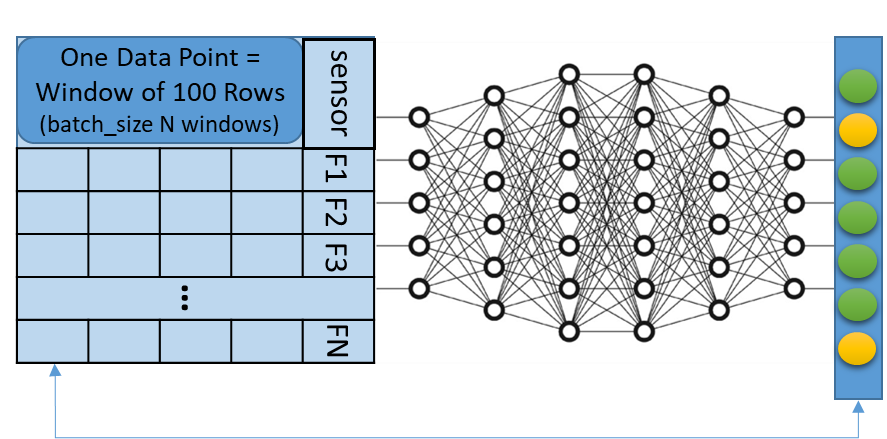
Figure 4: Single Expert

3.1.1 Frozen Single Experts

Each individual expert is pretrained as a current golden model; this allows for off-line training and competition of historical models against newer data as the dynamic nature of the dataset could change by the day or hour. These models comprise the initial layer of the GME architecture. This is an important feature as it allows for specific tuning and data segmentation based on the cyber-network being addressed, volume of data, and data types. In our experiments, we researched a variety of individual expert types, eventually settling on each individual sensor being its own expert type. Previously, we had also looked at dividing the data by subdomain, country, or protocol type, and having separate experts for each such division. But, such finer-granularity divisions were not found to provide significant benefits and the per-sensor expert was found to provide the best speed and accuracy. Each of our labels is based on data from a single sensor source; hence, per-sensor experts provide optimal performance in our setting. However, it should be noted that labels based on multiple sensor sources can be addressed in the system by segmenting the data appropriately allowing for a more complex label to exist in a single expert segmentation. Although the hyperparameters for each expert can be tuned separately, it was found that only minimal such tuning is required and training hyperparameters can be largely retained when moving to new sensor data types.

3.1.2 Batch Retrieval

Data for the GME was stored in a HDF5 database, which combines the sorted containers of data for each available sensor by time. Each individual sensor’s data is organized by time (minimally error-prone using 1 minute files and general commercial output accuracy). From these individual containers, a single sorted container is created prior to the GME running training or inference. As batches of windows are fetched across all sensors (or zeroed out), the individual expert layers receive a comparable time window for classification into the most probable classes. Batches are created with batch size and window as parameters.

3.1.3 Classification in the Gated Mixture of Experts

Given multiple sensor data sources, the data from the sensors are aligned over time windows as described above so that the window extracted from each sensor feed provides a view into the cyber-network’s operation over the same time range. With multiple sensors, the per-sensor experts operate as sensor-specific feature extractors, which are combined together using a gating mechanism. For this purpose, a separate light-weight gating network is trained that takes each sensor’s data and generates per-sensor scaling factors (which can be conceptually viewed as estimates of the importance of each sensor for classification in that particular time window). These scaling factors are then used to weight the outputs of the individual experts (i.e., to automatically determine which sensors are most relevant in that time window). The scaled combination of features is then passed into a fully connected layer followed by a softmax layer with binary cross entropy log loss function for training. The gating mechanism provides robustness to missing sensors or missing data in a time window. This is a crucial feature of the GME to allow decision making under periods of unobservable behavior. Given a time window of data, GME’s classification output for each row of data is either “Normal” or one or more labels. As rows of data are written out with label(s), this inherently allows for the most important rows contributing to higher order named threat classes to pass through. This was shown to filter the dataset from over several terabytes to 100’s of gigabytes while preserving a mapping index into the full raw dataset. These classifications should be viewed as enrichment data points versus malicious or even suspicious elements on their own. The classification by a machine learning algorithm provides an alternative to database heuristics as the machine learning adds elements of both fuzzy matching (multi-field labels) and threshold finding (continuous fields). The labels output by GME are cross-correlated further down the data flow pipeline in ESAFE by the post-processing module (including cross-correlation across multiple sensors to construct more complex labels).

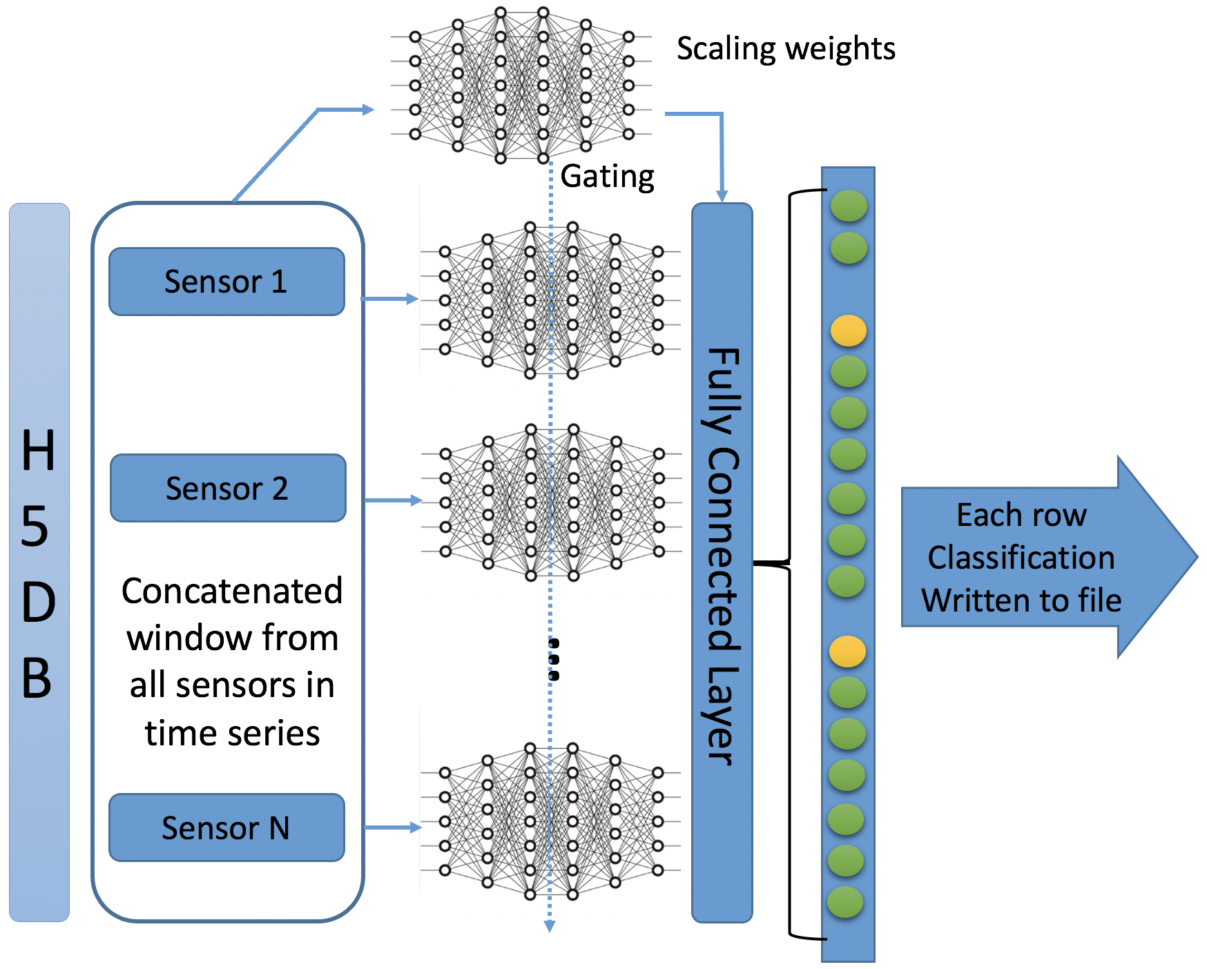
Figure 5: Gated Mixture of Experts Architecture

3.2 Probabilistic Parameterized Metric Temporal Logic

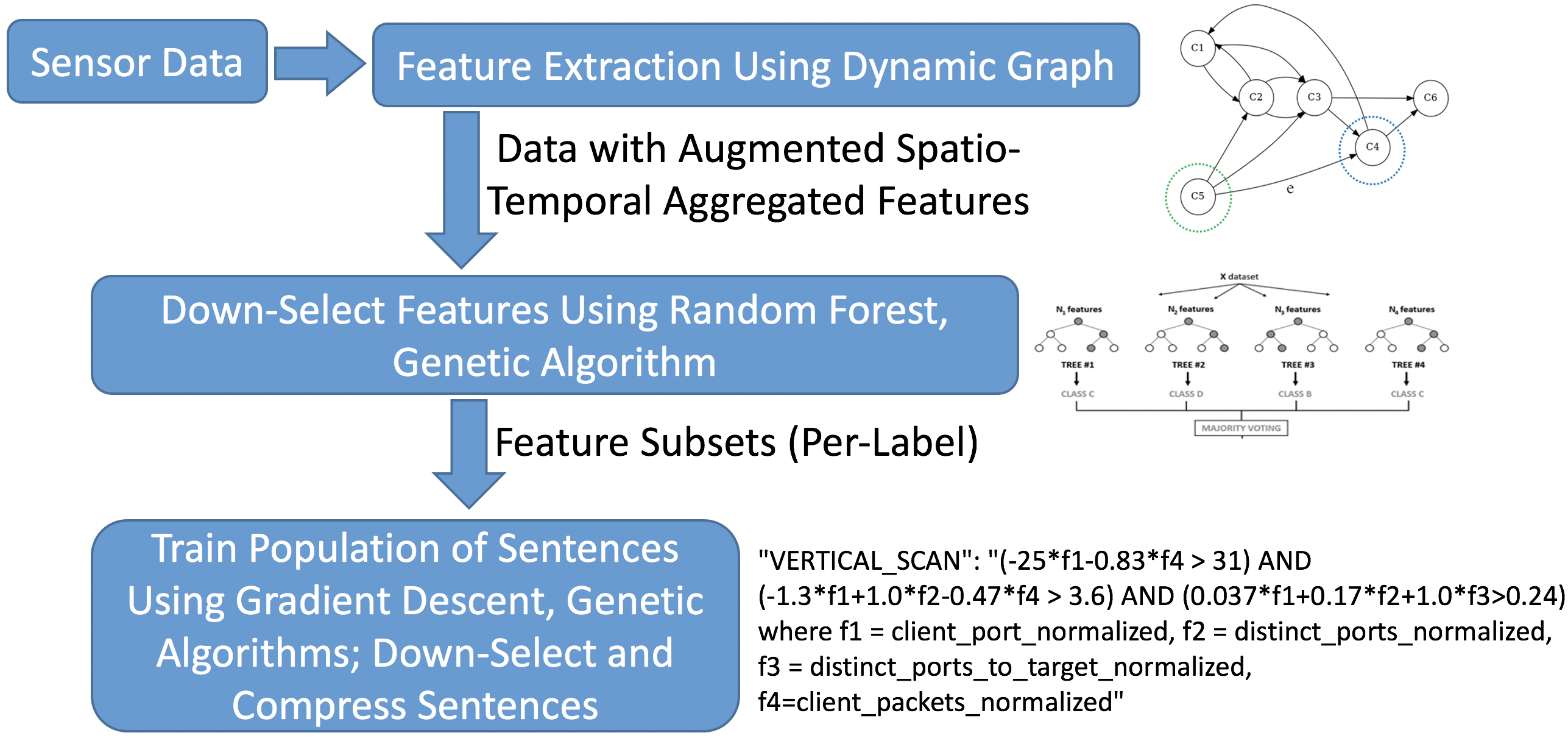
Figure 6: Human Readable Architecture

The ppMTL module (Figure 6) in ESAFE can run in two modes: a light-weight mode in which the features relevant to a classification of a particular label are identified and a full mode in which additionally a human-readable representation of the decision logic is generated as a set of linear inequalities in terms of the identified features. The ppMTL module in ESAFE plays a complementary role to the GME module. While the GME addresses at-scale classification from input data, the ppMTL module addresses the generation of human-readable annotations. Hence, in one configuration, the ppMTL module is only fed the rows that GME marks as non-normal, i.e., the rows that the GME associates with at least one label. For these rows, the ppMTL module then generates human-readable annotations. Since the ppMTL module also internally generates per-class likelihoods for input rows as part of the generation of human-readable annotations, the other configuration possibility is to feed all input data rows to ppMTL and then probabilistically fuse the outputs of GME and ppMTL using, for example, a Bayesian per-class ensemble classifier. The choice between these two configurations is primarily one of scale with the former being more computationally efficient to address very large amounts of data. In either configuration, the main role of ppMTL is to provide greater visibility into the system for the human analyst as compared to raw probability vectors indicating likelihoods of different labels and to instead be able to provide an insight into why a given label fired.

3.2.1 Spatio-Temporal Feature Extraction Using a Dynamic Graph

To facilitate representation of decision logic in terms of human-interpretable quantities, a spatio-temporal aggregation approach is utilized to construct features that summarize various aspects of network activity from the viewpoints of specific nodes (IP addresses) in the network. This is crucial since the underlying “reasons” for why a particular row in sensor data is classified as a particular label could be related to events represented in multiple spatially/temporally separated rows in the sensor data. Hence, simply presenting raw sensor data does not provide much insight into why a particular label fired; instead, it is crucial to highlight the aggregates among the rows that together explain why the label fired. In the context of network log data, spatio-temporal aggregations include, for example, quantities such as statistics of incoming and outgoing packets and bytes at each node and between pairs of nodes (e.g., total, max, average, number of distinct ports), numbers of distinct nodes with which a node has communicated over a sliding time window, numbers of distinct ports over which a node has communicated over a sliding time window, etc. A dynamic graph structure (with graph nodes being network nodes represented as IP addresses and graph edges being communications between network nodes) is used to efficiently ingest and process the streaming sensor data. The dynamic graph is iteratively constructed from the streaming sensor data and provides a framework to instantiate new nodes and edges depending on observed network activity, maintain a sliding time window memory, dynamically remove nodes and edges based on configurable forgetting rules, and enable computation of spatio-temporal aggregation based features as queries answerable by nodes and edges in the graph (by consulting adjacent/nearby nodes and edges as required for specific spatio-temporal aggregations).

3.2.2 Feature Down-Selection Using Random Forest and Genetic Algorithms

To determine the subset of features (including features present in original sensor data and features constructed using spatio-temporal aggregations) that are most relevant for classification of each label, a random forest classifier is used as an efficient per-class feature utility estimator and a genetic algorithm is used as a search algorithm in the space of possible feature subsets. While other classification algorithms could also be used instead for this purpose, a random forest classifier has the advantage that it intrinsically generates (as part of training) feature utility/relevance estimates (feature “importances”), which are directly provided by highly optimized off-the-shelf implementations, and is therefore used for feature utility estimation in this implementation. For each label, starting from a randomly initialized population of candidate solutions (choices of subsets of features), each candidate solution is evaluated to form two metrics: firstly, the classification $F_{1}$ score on a test dataset when the classifier for that label is trained using only the subset of features in that candidate solution; secondly, the utility of each feature within the candidate solution as estimated by the random forest classifier during training. The fitness of a candidate solution is defined as a composite of the classification $F_{1}$ score and a penalty based on the number of features appearing in that candidate solution (with a pre-specified constraint on max number of features; e.g., 5 in our experiments). Genetic operators for random mutations and cross-overs are defined to favor picking candidate solutions of higher fitness and features therein of higher feature utilities. The subset of features identified as most relevant for each label is used to learn a set of human-readable sentences as discussed below that characterizes the classification decision logic for that label.

3.2.3 Learning of Human-Readable Sentences

For each label, based on the subset of relevant features identified as discussed above, a set of human-readable sentences (with each sentence comprised of an AND-combination of a set of linear inequality based conditions, each of which is called a “word” in the sentence) is learned using a combination of stochastic gradient descent and genetic algorithms (Krishnamurthy et al. (2021)). This component of ppMTL is enabled only when ppMTL is run in “full” mode and is not enabled in the “light-weight” mode in which the feature down-selection discussed above provides the required identification of the subset of features. The learning of the human-readable sentences addresses two problems: learning of which features to use in each inequality (as defined by a binary mask over the set of all features) and learning of coefficients in the inequalities. The union of the set of all sentences learned for a label characterizes (via an OR-combination) the volume in feature space corresponding to the label. Discrete-valued features (i.e., features that can take only a relatively small number of possible values, e.g., Boolean-valued features) are encoded into continuous-valued proxy features based on, for example, relative frequencies of the appearance of the possible values for the features.

To enable gradient-based learning of the coefficient variables, a differentiable relaxation of the OR-of-AND structure of the set of sentences is used based on sigmoid functions and replacement of Boolean operators by product (for AND) and max (for OR) operators. The loss function for training is defined as a combination of the binary cross-entropy, a penalty term for false positives, and a regularizer penalizing the magnitudes of the coefficient variables and number of non-zero entries in the mask variables. In parallel with the learning of the coefficient variables using stochastic gradient descent (e.g., every some pre-defined number of epochs of gradient-based updates), the mask variables are updated using a genetic algorithm based on a fitness model for sentences. The fitness of a sentence is defined as a combination of the classification performance of the sentence as measured by the rates of true positives and false positives and the sentence complexity (based on the number of features appearing in the sentences). The set of sentences is randomly initialized, fine-tuned using gradient-based updates, and evolved using randomized mutation and resampling operators based on the computed fitness values of the sentences.

After the sets of sentences are learned for each label, these sets are pruned using a sentence down-selection algorithm to determine the subsets of sentences that are adequate to represent the learned model and each retained sentence is compressed to remove redundancies in the constituent inequalities and determine a more compact representation of the sentence. Once separate models are learned for each anomaly/threat type, inter-label correlations (i.e., between different anomaly/threat types) can be integrated based on any known inter-dependencies between labels (e.g., due to semantic interrelationships between labels) and learning of a meta-classifier model to map the activation outputs of the classifiers for each of the labels into the final outputs for the labels.

3.2.4 Human Readable Output

Based on the learned feature subsets and sentences as discussed above, the ppMTL module can identify, during inference, the features and linear inequality based combinations thereof for each specific row in sensor data classified as a particular label. The ppMTL module can also identify the composite of all relevant features and linear inequality conditions for all data points classified as that label (i.e., the union of human-readable annotations which serves as a description of the overall decision logic for that label). The ppMTL module’s human-readable annotation outputs for each row classified as a particular label are passed to an ancillary database that is queryable by an analyst or post-processing module for further downstream use. While multiple sentences could fire for a particular row, ppMTL automatically picks the best sentence based on sentence compactness and classification performance metrics. The selected sentences provide context-aware explanations for the classification by identifying the specific set of conditions that were satisfied by each data point marked as a particular label.

4 System Architecture

The ESAFE system is a hierarchical reasoning system comprised of layers of data storage, collection and preprocessing, machine learning based classification using the GME and ppMTL, and finally postprocessing over the final output before transforming it into the desired UI.

4.1 Pre-Processing

The ESAFE system is designed to ingest a variety of data types from a variety of data sources. Furthermore, it is designed to be extensible, so that new data types and data sources can be added without re-implementing the machine learning and clustering components of the system.

In order to support such a wide variety of data types and sources, as well as to ensure extensibility, the data must be pre-processed into a common format that can be consumed by subsequent components.

The Pre-Processing stage comprises the following steps:

1. Identify available data types.

2. Define a schema for each data type.

3. Collect the raw data from one or more data sources.

4. Convert the raw data into one or more standardized formats that correspond to the schema for that data type.

5. (Optional) Label the data.

Each of these steps is discussed in further detail below.

4.1.1 Identifying Available Data Types

The ESAFE system is designed as a general framework for processing cyber-relevant data from a variety of data sources. ESAFE does not perform data collection on its own; instead, it relies on data that has been collected by other tools (aka “data sources”), such as Bro/Zeek, NetFlow, Windows Event Logs, firewall logs, etc.

Consequently, one of the first steps is to identify the data types that the system will process. For our purposes, a “data type” is a record with a consistent schema that is generated by a specific monitoring tool. The following are examples of some data types that are supported by the ESAFE system:

1. Bro/Zeek Conn logs

2. Bro/Zeek SSH logs

3. NetFlow records

4. Active Directory event logs

5. Web Firewall event logs

4.1.2 Collecting Raw Data

A particular concern at this step is how to retrieve the data at scale. Some data types, such as Bro/Zeek Conn logs and NetFlow logs, are voluminous, so care must be taken to ensure that the system can retrieve the raw data for the desired time range in a reasonable period of time. In one environment, this was achieved by designing the code to take advantage of the compute resources that were available to individual virtual machines (32 vCPUs, up to 256GB of RAM, 2TB of disk, etc.). In another environment, this was achieved by leveraging the available high-performance computing (HPC) resources; generally, this meant breaking the retrieval task up into dozens or hundreds of very small tasks that could all be run independently in parallel.

There is no single approach that will be optimal for all deployment environments. Regardless of how the raw data is ultimately collected, it must then be converted into a format which corresponds to the appropriate schema for the data type, and then exported into one or more common formats that can be leveraged by downstream components.

During development, it became clear that the labeling component and the cluster hunting component relied heavily on the time-ordering of data. Consequently, the performance of downstream components can be improved (at times dramatically) by ensuring that when data is written out, it is written out sorted by time.

4.1.3 Labeling the Data

Once the data has been exported to a standard format for processing, it can optionally be labeled. Labeling rules can vary dramatically in terms of the complexity of their implementation. When developing the ESAFE system, we considered the following types of labels:

1. A label which operates on a single row of data. This is the most scalable type of label.

2. A label which operates on a relatively small window of data, such as 100 to 1000 rows, from the same file. This type of rule generally scales well.

3. A label which operates on a “large” window of data of the same data type, where “large” will vary based on data type. Typically, anything that will require tens of thousands of rows (or more) split across multiple files would fit in this category. In general, this type of rule is more difficult to scale.

4. A label which operates on multiple data types at once. In this study, we did not implement labels of this type.

These are discussed in greater detail below.

4.1.4 Labeling Single Rows of Data

The easiest and most scalable types of labels to apply are labels that can be derived from examining one row of data at a time. For labels such as these, the labeling task can be broken down into hundreds of smaller labeling tasks which can then be submitted as a batch job on a HPC system. These rules are also easier and faster to implement, as well as less prone to errors (bugs), because they do not need to maintain state.

However, these labels are also generally the least “interesting” from an analyst’s perspective.

4.1.5 Labeling Based on Small Windows

Labels that are applied based on “small windows” of data can provide much of the scalability benefits of single-row-based labels while allowing for more complexity (and analyst utility). Typically, windows that are defined in terms of a fixed number of rows (e.g., 1000 rows) are the most scalable and easiest to implement; windows that are defined in terms of a fixed period of time (e.g., 10 seconds) can be more difficult to implement, because for some data types, such as Bro/Zeek Conn logs, 10 seconds of data could represent hundreds of thousands of rows; furthermore, when windows are defined in terms of time, there is often a greater likelihood that the data will be split across multiple files.

Nevertheless, some labels may require time-based windows due to their nature. As discussed before, the performance of such labels will typically benefit if the data was exported in time-series order (i.e., sorted by time).

4.1.6 Labeling Based on Large Windows

As a general rule, labeling based on “large windows” (either millions of rows or hours of data) will require a more sophisticated back-end data store. Typically, in order to apply such labels in a timely manner, the system will need to leverage a data store that supports queries. Scalability in labeling when using large data windows remains an open topic of research.

4.2 Cluster Hunting and Post-Processing

Once the data has been labeled (enriched) and filtered by the GME and the ppMTL, numerous data science and analytical techniques can be applied to search for suspicious and malicious behavior during cluster hunting:

1. Describe a type of malicious behavior that is to be searched for in the data.

2. Identify artifacts that would be left in the available logs from such behavior.

3. Apply a label indicating each such artifact.

4. Define a “cluster” of such labels which indicate that behavior. Minimally, a cluster would be a group of labels that appear in a specific order within a particular time window. Typically, clusters will have additional constraints, such as the labels being applied to the same source or destination IP addresses, or the same TCP or UDP ports, etc.

5. Search for all defined clusters in the labeled data.

6. Report each detected cluster via an appropriate mechanism, such as a report, a log entry, a ticket submitted to a ticketing system (such as Redmine), etc.

Steps 1-4 were the focus of Section 3 while steps 5-6 are explored in more detail below.

4.2.1 Label Artifacts

Once 3-5 artifacts have been identified that are associated with a class of malicious behavior, it will need to be ensured that each artifact label exists in the pre-processing of data. If such labels do not already exist, they will need to be added. Adding new labels to the system can be time-consuming, since it requires re-labeling training and test data, and then re-training the GME and ppMTL. However, one of the strengths of the Cluster Hunting approach is that the same label can appear in any number of clusters; so it will not necessarily be required to define a new label whenever a new cluster is added to the system. For example, two different clusters might both include an underlying label such as HTTP_REDIRECT.

4.2.2 Search for Clusters

If a data store is available which supports a sophisticated query language, such as SQL, then it may be possible to formulate the cluster logic as a single query to the system. Assuming that a suitable, query-able data store is not available, the labeled data files will need to be searched. During our experiments, we also found that removing rows from the data set which did not have labels that occurred in at least one cluster could substantially reduce the overall volume of data that needed to be searched. In one case, we were able to reduce the overall volume of data for a particular data type by half. This is often the case with a “Normal” label— i.e., a label which represents a row that has no other label. Since the “Normal” label never occurred in any of our cluster definitions, we were able to reduce the overall search space by half simply by eliminating rows that had been labeled “Normal”.

4.2.3 Report Detected Clusters

The appropriate mechanism to report detected clusters will vary based on the deployment scenario. Some analysts will simply want a report, such as a text file, to describe the detected cluster. Other scenarios may require exporting the cluster in a machine-consumable format, such as JSON file. Other scenarios may involve publishing the detected cluster to a message channel, such as Apache Kafka, for use by downstream software. And still other workflows may require posting the detected cluster as an issue to an issue tracker or ticketing system, such as Redmine.

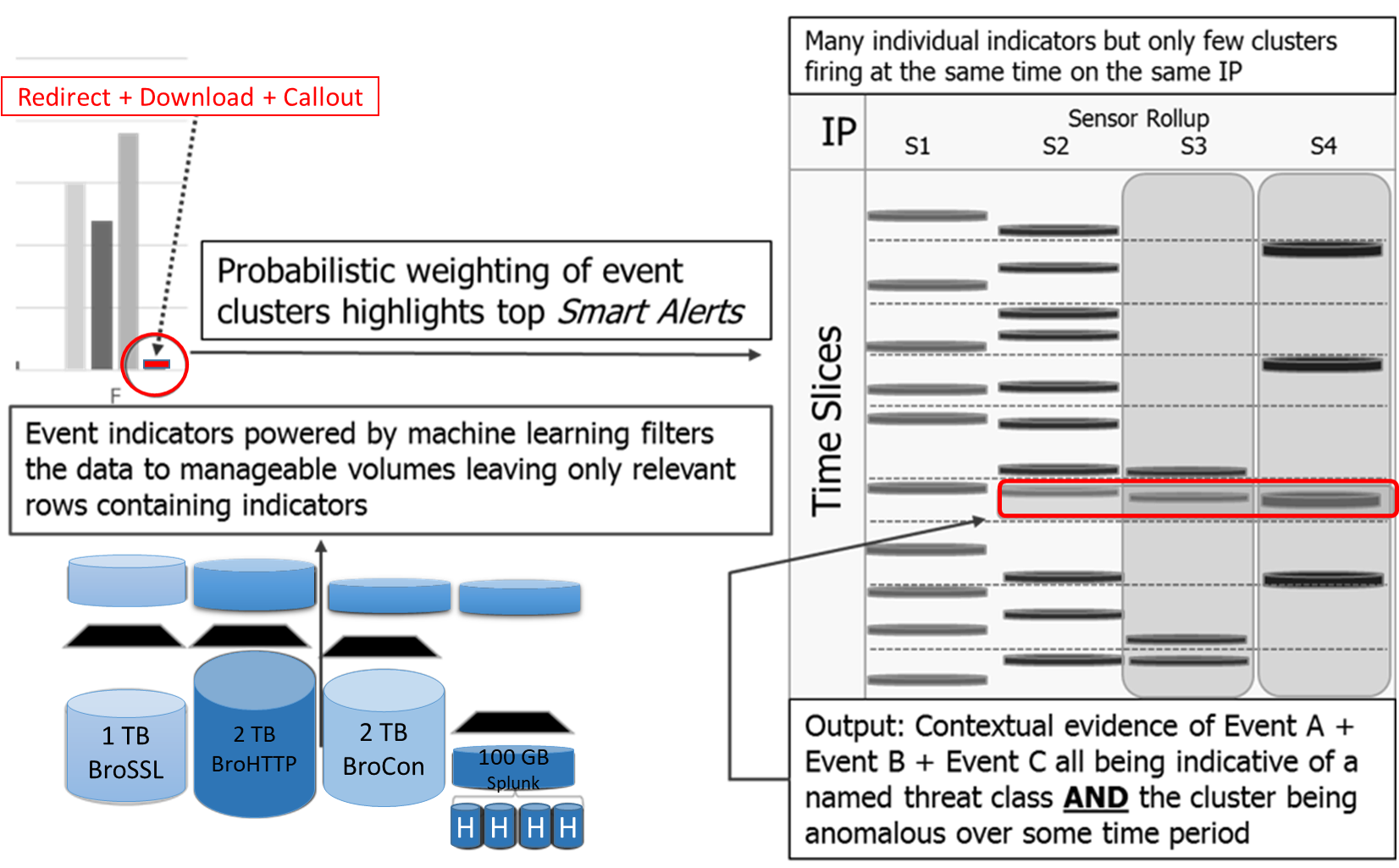
Figure 7: Smart Alert Flow

In general, the cluster hunting system should be designed in such a way as to support exporting detected clusters to a variety of export formats. As with the Collecting Raw Data step in the Pre-Processing stage, this is likely to be a part of the system that requires a nontrivial degree of environment-specific (Strayer et al. (2009)) development. (Tan and Maxion (2002)).

5 Lessons Learned

We have four key lessons learned we wish to highlight:

1. We must know when we need more data and where it should be collected. This follows “The essence of the CHASE program is how do you get the right data from the right device at the right time in order to really bolster our security in our networks.” (Williams (2019)).

2. Logs may not contain all the data needed to make a determination between conclusions when there are two possible explanations for our cluster of elemental rules alerting.

3. There is no single one best labeling strategy and we need a moderated approach where we have enough elemental rules to have clusters which are explainable to the user and able to find new attacks.

4. A short time window is not sufficient to alert, any threat that takes longer than the time window simply will not fire enough elemental labels to make a cluster we can make a determination on. We did by hand cover larger time windows to adapt to this limitation.

6 Open Challenges

Inconclusive ESAFE reports is our greatest current short fall. We have on numerous occasions been left with the conclusion that there are two possible explanations for our cluster of elemental rules alerting (e.g., have we observed a watering hole attack or has there been a redirect to a previously unseen server? have we observed a DDOS attack or is there a Bro logging error/misconfiguration?). False positives where alerts are generated since our cluster label(s) have hit but with inconclusive supporting data result in the Analyst having to spend a large amount of time to investigate the flagged anomalies. This is a very cost intensive process and quickly leads to diminishing returns for the SOC Analyst. Anomalies, particularly in network traffic, do not necessarily equate to malicious behavior. The noise floor and the flux in user behavior both contribute to this effect. This opens the question: was information available sufficient to determine which of two hypotheses is correct? In cases of ambiguity, we must infer the data we need to resolve the ambiguity and collect such data. Waiting for the data to make a decision, benign or malicious, to arrive is not necessarily a correct approach for two main reasons:

1. The data we want may never be transmitted.

2. Attackers often run campaigns over long periods of time to avoid detection. Since attacks would take a long period of time to manifest, it means the number of hypotheses can grow to an unmanageable scale forcing us to stop tracking. In either case, many attacks can be missed.

For future work, we recommend two main avenues: firstly, the category of suspicion should be adopted, in order to bridge the semantic and information gap; secondly, a study of the information loss from raw data (e.g., pcap) to logs (e.g., bro_ssl_logs) needs to be performed.

6.1 Study Information Loss from raw data to logs

All of our elemental labels reason over logs and when ESAFE reports back, the highest degree of fidelity of evidence that can be provided is row(s) of data with columns of interest included. Currently, SOCs investigate alerts and pivot as necessary to obtain supporting information. The analyst knows what information is relevant and from what source or sources to obtain it. Future work should apply information theoretic approaches to quantify what information is lost at each stage of collection and what information is needed to make a determination for each elemental rule and cluster label. Logs from sensors are not intended to be complete forensic archives of network traffic. In fact, they are by definition and construction a summary of the expected behavior.
As a motivating example, we see the need to cluster information-aware rules: Let us consider a Bro_SSL_Log and Artifacts from the set ”TTP” _(TLS_encrypt_c2), where the JA3 hash is present in an SSL Log, the client_hello information has been hashed (via MD5) and thus extracting similarities from the artifacts is not possible from the log. Since real browsers support $\sim$40 encryption methods, logging of all client_hello strings would collect too much data resulting in log storage problems.

In accordance with the CHASE model, information-aware rules are used for finding similarities of client_hello strings to known malware samples. We would need to request this data (via pcap) iff a threshold for suspicion is met for a specific server; this data would not be stored after comparison. This work should be approached by describing what information is captured by each log and what information is present but not captured. Elemental rules should clearly include in their automated report what information is needed to make a determination, but was not present (Barreno et al. (2006)).

6.2 Suspicion

Even with high fidelity in the information that is present in log(s) and that is available from raw data, many alerts will not be resolved in a rolling time window. The concept of a system being suspicious should be introduced. When sufficient data (e.g. logs, raw) to resolve if an alert is malicious is not available, such suspicions must still be presented to the analyst for their interpretation and not simply dismissed.

There are some mitigating steps ESAFE should explore, such as additional targeted information via raw collection. This should be done in two ways; with respect to the systems involved in the alert, more data requested by ESAFE and with respect to the network the meta-statistics of alert clusters should also be tracked. ESAFE should also track when new elemental labels appear in clusters they have not been seen in previously, or when more data is requested by ESAFE than had previously been needed for a cluster alert. In other words, ESAFE must track how cluster alerts are currently being used and how they are changing.

References

- Barreno et al. [2006] Marco Barreno, Blaine Nelson, Russell Sears, Anthony Joseph, and J. Tygar. Can machine learning be secure? In Proceedings of the ACM Symposium on Information, Computer and Communications Security, pages 16–25, Taipei, Taiwan, March 2006.
- Krishnamurthy et al. [2021] Prashanth Krishnamurthy, Alireza Sarmadi, and Farshad Khorrami. Explainable classification by learning human-readable sentences in feature subsets. Information Sciences, 2021. Accepted for publication, early access version available Feb. 2021.
- Sommer and Paxson [2010] Robin Sommer and Vern Paxson. Outside the closed world: On using machine learning for network intrusion detection. In Proceedings of the IEEE Symposium on Security and Privacy, pages 305–316, Oakland, CA, May 2010.
- Strayer et al. [2009] Tim Strayer, Walter Milliken, Ronald Watro, Walt Heimerdinger, Steven Harp, Robert Goldman, Dustin Spicuzza, Beverly Schwartz, David Mankins, Derrick Kong, and Pieter Zatko. An architecture for scalable network defense. In Proceedings of the IEEE Conference on Local Computer Networks, pages 368–371, Zurich, Switzerland, Oct. 2009.
- Tan and Maxion [2002] K. M. C. Tan and R. A. Maxion. “Why 6?” Defining the operational limits of stide, an anomaly-based intrusion detector. In Proceedings of the IEEE Symposium on Security and Privacy, pages 188–201, Oakland, CA, May 2002.
- Williams [2019] Lauren C. Williams. DARPA has big plans for the CHASE program, 2019. Available online on Defense Systems: https://defensesystems.com/articles/2019/03/08/darpa-chase-cyber-williams.aspx?m=1#:~:text=Developing%20proven%20cyber%20defense%20tools,protect%20multiple%20DOD%20enterprise%20networks.