Isoharmonic deformations and constrained Schlesinger systems

Abstract

We introduce and study the dynamics of Chebyshev polynomials on $d>2$ real intervals. We define isoharmonic deformations as a natural generalization of the Chebyshev dynamics. This dynamics is associated with a novel class of constrained isomonodromic deformations for which we derive the constrained Schlesinger equations. We provide explicit solutions to these equations in terms of differentials on an appropriate family of hyperelliptic curves of any genus $g=d-1\geq 2$. The verification of the obtained solutions relies on the combinatorial properties of the Bell polynomials and on the analysis on the Hurwitz spaces. From the point of view of the classical algebraic geometry we formulate and solve the problem of constrained Jacobi inversion for hyperelliptic curves. We discuss applications of the obtained results in integrable systems, e.g. billiards within ellipsoids in $\mathbb{R}^{d}$.

MSC: 30F30, 31A15, 32G15 (35Q07, 14H40, 14H70)

Keywords: polynomial Pell’s equations; Chebyshev polynomials; hyperelliptic T-curves; isoharmonic deformations; constrained Schlesinger equations; Bell polynomials; Rauch variational formulas.

Dedicated to the bicentennial of birth of P. L. Chebyshev (1821-1894), the founding father of the modern St. Petersburg school of mathematics.

1 Introduction

Let us consider $d$ real intervals with $d>2$ and a point $y_{0}$ in the extended complex plane outside the intervals. A harmonic measure with a pole at $y_{0}$ is assigned to each of these $d$ intervals (see e.g. [53]). In this paper we introduce and study deformations of the endpoints of the intervals and of the position of the pole $y_{0}$ in a way that the harmonic measures of these deformed $d$ intervals with respect to the deformed pole $y_{0}$ remain unchanged under the deformation. We will call such deformations isoharmonic and understand them as deformations of a pair formed by a region and a point in it. Here, the region is the complement of the union of $d$ intervals in the extended complex plane and the point is the position of the pole $y_{0}$.

Since we assume that $d>2$, there is a hyperelliptic curve of genus $g=d-1\geq 2$ obtained as a double covering of the Riemann sphere ramified over the $2d$ endpoints of the intervals. The position $y_{0}$ of the pole of the harmonic measures defines two points $Q_{0},Q_{0}^{*}$ on the curve, paired by the hyperelliptic involution, lying above $y_{0}$ on the double covering. The isoharmonic deformations along with their interpretation in potential theory also carry a transparent algebro-geometric meaning by inducing special deformations of the hyperelliptic curve, and are related to a class of isomonodromic deformations of linear systems.

Let us first discuss the algebro-geometric context. Assuming one of the endpoints of the intervals to be the point at infinity, the isoharmonic deformations determine a smooth family of hyperelliptic curves together with a section consisting of the points $Q_{0}$. More precisely, we will define a smooth family of hyperelliptic curves $\hat{T}:\hat{\mathcal{H}}\to\hat{X}$ parameterized by the parameter set $\hat{X}$ introduced below (see Sections 2, 3, and Definition 2 in Section 5.1). The fiber $\mathcal{H}_{\bf x}$ over ${\bf x}\in\hat{X}$ is the projective closure of the algebraic curve of the equation

$$\mu^{2}=\Delta^{{\bf x}}_{2d-1}(z),$$ (1.1)

where $\Delta^{{\bf x}}_{2d-1}$ is a polynomial of degree $2d-1$. Taking a small enough neighbourhood $\hat{X}^{0}$ of ${\bf x^{0}}\in\hat{X}$ we can choose a canonical homology basis in a consistent way for all curves $\mathcal{H}_{\bf x}$ with ${\bf x}\in\hat{X}^{0}$ by requiring that the projections of the basis cycles to the $z$-sphere be independent of $\bf x$. There is also an induced vector bundle $V\to\hat{X}^{0}$ whose fiber over $\bf x$ is the vector space of holomorphic differentials on the curve $\mathcal{H}_{\bf x}$. Fix a basis of sections of this bundle normalized with respect to the $\bf a$-cycles of the chosen canonical homology basis. Let us base the Abel map at the point at infinity $P_{\infty}$ of each curve. Then, there exists a section $s_{Q_{0}}$ of the family $\hat{T}$ of the hyperelliptic curves, such that

$$\mathcal{A}_{P_{\infty}}(s_{Q_{0}}({\bf x}))=\hat{c}_{1}+\mathbb{B}_{\bf x}\hat{c}_{2}.$$ (1.2)

Here $\mathbb{B}_{\bf x}$ is the Riemann matrix of $\mathcal{H}_{\bf x}$ for the given choice of the homology basis and $\hat{c}_{1},\hat{c}_{2}\in\mathbb{R}^{g}$. Then the isoharmonicity of the deformations implies that $\hat{c}_{1},\hat{c}_{2}$ are constant vectors independent of ${\bf x}\in\hat{X}^{0}$. By applying to $s_{Q_{0}}$ the hyperelliptic involution in the fibers, we get the associated section $s_{Q_{0}^{*}}$ of $\hat{T}\,.$

The isoharmonic deformations are closely related to the theory of isomonodromic deformations of linear differential systems. In order to articulate and explore this relationship, we introduce a novel class of isomonodromic deformations of Fuchsian systems, the so called constrained isomonodromic deformations. Some constrained isomonodromic deformations are described by solutions to the constrained Schlesinger system. We construct explicit families of such deformations in terms of differentials of the third kind on the fibers of the family $\hat{T}$ of hyperelliptic curves with simple poles along sections $s_{Q_{0}}$ and $s_{Q_{0}^{*}}$. In each fiber, the periods of the differential with respect to the chosen homology basis are constant multiples of $\hat{c}_{1},\hat{c}_{2}$. Thus, the periods are constants independent of the fiber. The bridge connecting the potential theory side with the algebro-geometric framework is the fact that the above differentials of the third kind correspond to the differentials of the Green functions of the complement of the union of $d$ intervals with the pole at $y_{0}$. The independence on the fibre of the periods of the differentials then relates to variations of the region and the pole in an isoharmonic way.

A section of a family of elliptic curves defined by the condition (1.2) with fixed constants $\hat{c}_{1},\hat{c}_{2}$ arose in the context of isomonodromic deformations in the classical work of Picard [49]. Picard provided a general solution of one of the Painlevé VI equations more than a decade prior to works of Gambier [26] and of R. Fuchs [33], who derived the general form of such equations. The Painlevé VI equation is a second order ordinary differential equation with parameters $\alpha,\beta,\gamma,\delta\in\mathbb{C}$, denoted PVI$(\alpha,\beta,\gamma,\delta)$, see eg. [47], [34], [41]. R. Fuchs derived it in 1907 [33] in his study of isomonodromic deformations of a Fuchsian linear system with four singularities at $\{u_{1}=0,u_{2}=1,u_{3}=x,u_{4}=\infty\}\subset{\mathbb{CP}}^{1}$

$$\frac{d\Phi}{du}=A(u)\Phi,\qquad u\in{\mathbb{C}},$$ (1.3)

for a $2\times 2$ matrix function $\Phi(u)$ defined in the complex plane, where the matrix $A\in sl(2,{\mathbb{C}})$ is of the form:

$$A(u)=\frac{A_{1}}{u}+\frac{A_{2}}{u-1}+\frac{A_{3}}{u-x}.$$

As was already known to Painlevé in 1906 and rediscovered by Manin in [41], the Painlevé VI equations have an equivalent elliptic form:

$$\frac{d^{2}\,z}{d\,\tau^{2}}=\frac{1}{2\pi i}\sum_{j=0}^{3}\alpha_{j}\wp_{z}\left(z+\frac{T_{j}}{2},\tau\right),$$

where the transformed Weierstrass $\wp$-function satisfies: $(\wp^{\prime}(z))^{2}=\wp(z)\;(\wp(z)-1)\;(\wp(z)-x)$ and the parameters are related by:

$$(\alpha_{0},\alpha_{1},\alpha_{2},\alpha_{3})=(\alpha,-\beta,\gamma,1/2-\delta).$$

Let $\mathcal{E}_{x}$ be an elliptic curve represented as a two-fold covering of the Riemann sphere ramified over the set $\{0,1,x,\infty\}$ with $x\in\mathbb{C}\setminus\{0,1\}$. For some chosen canonical homology basis, let the Abel map be based at the point at infinity and let the Jacobian be generated by the Weierstrass vectors $2w_{1},\,2w_{2}\in\mathbb{C}$. Then $T_{j}$ are the periods $(0,2w_{1},2w_{2},2w_{1}+2w_{2})$.

Now we can say more about the general solution of the Picard equation, which is the Painlevé VI equation with parameters $(\alpha_{0},\alpha_{1},\alpha_{2},\alpha_{3})=(0,0,0,0)$, that is PVI$(0,0,0,1/2)$. Let us fix an arbitrary point $z_{0}$ in the Jacobian of $\mathcal{E}_{x}$. Then $z_{0}=2w_{1}\hat{c}_{1}+2w_{2}\hat{c}_{2}$ for some $\hat{c}_{1},\,\hat{c}_{2}\in\mathbb{R}.$ The Jacobi inversion of $z_{0}$ gives a point $Q_{0}\in\mathcal{E}_{x}$ for which the projection on the base of the two-fold ramified covering is given by the image of $z_{0}$ under the Weierstrass $\wp$-function, $y_{0}=\wp(z_{0}).$ If we now allow $x$ to vary, assuming that the projection of the homology basis on the base of the covering stays fixed, we need to define the corresponding variation of $z_{0}.$ The natural way to define this variation is the one leading to the Picard solution: $z_{0}$ is defined to be the point given by the above equality with $\hat{c}_{1}$ and $\hat{c}_{2}$ being fixed for all curves $\mathcal{E}_{x}$, that is $z_{0}(x)=2w_{1}(x)\hat{c}_{1}+2w_{2}(x)\hat{c}_{2}$ with $\hat{c}_{1},\hat{c}_{2}$ independent of $x$. This gives the Picard solution $y_{0}=\wp(z_{0}(x))$ of PVI$(0,0,0,1/2).$

In other words, we have a family of elliptic curves $\pi:\mathcal{E}\to\mathcal{B}_{0,1}$ over the set $x\in\mathcal{B}_{0,1}:=\mathbb{C}\setminus\{0,1\}$ with a fiber given by an elliptic curve $\mathcal{E}_{x}$ as above. Points at infinity of the elliptic curves form a section of $\mathcal{E}$ which is taken as the zero for the group law on the fibers. The points $Q_{0}$ defined as above form a local section $s_{Q_{0}}$ of $\mathcal{E}$.

We can then define a differential $\Omega$ of the third kind on $\mathcal{E}_{x}$ with a simple pole of residue $+1$ along the section $s_{Q_{0}}$ and a simple pole of residue $-1$ along the section $s_{Q_{0}^{*}}$ obtained from $s_{Q_{0}}$ by the elliptic involution of $\mathcal{E}_{x}$ interchanging the sheets of the covering; let the differential be normalized by the condition that its $a$-period with respect to the chosen homology basis is equal to $-4\pi{\rm i}\hat{c}_{2}\,.$ It turns out, see [18] and [32], that the two zeros of $\Omega$, paired by the elliptic involution, form a local section of the family $\pi$ of elliptic curves whose projection on the base of the two-fold coverings representing the curves, seen as a function of $x\in\mathcal{B}_{0,1}$ coincides with the solution of PVI$(\frac{1}{8},-\frac{1}{8},\frac{1}{8},\frac{3}{8})\,$. The constants $\hat{c}_{1},\hat{c}_{2}$ play the role of the initial condition for the differential equation. Moreover, the relationship between the poles and zeros of $\Omega$ is given by the Okamoto transformation between solutions of PVI$(0,0,0,\frac{1}{2})$ and PVI$(\frac{1}{8},-\frac{1}{8},\frac{1}{8},\frac{3}{8})\,$, see also [40].

Our objective now is to find a counterpart of solutions to PVI$(0,0,0,\frac{1}{2})$ and PVI$(\frac{1}{8},-\frac{1}{8},\frac{1}{8},\frac{3}{8})\,$ in the case of a family of hyperelliptic curves. Thus, our starting point is to find an analogue of the Picard solution for hyperelliptic curves. Given that the Painlevé VI equations describe isomonodromic deformations of linear systems (1.3), where the parameters $(\alpha,\beta,\gamma,\delta)$ are related to the eigenvalues of the residues of the matrix $A(u)\,,$ it is natural to expect that, for the sake of possible generalizations, the role of the Painlevé VI equation is played by the Schlesinger systems. Recall that the Schlesinger systems give the dependence of the residue matrices of $A(u)du$ on the positions of Fuchsian singularities of linear system (1.3), with an arbitrary number of singularities, such that the linear system be isomonodromic.

Suppose now that we have a family $T:\mathcal{H}\to X$ of hyperelliptic curves of genus $g>1$ over some parameter space $X$ where we can choose the canonical homology bases consistently for all the curves. Following the logic of the Picard solution, let us fix $\hat{c}_{1},\hat{c}_{2}\in\mathbb{R}^{g}$ and consider a point $z_{0}=\hat{c}_{1}+\mathbb{B}_{\bf x}\hat{c}_{2}$ in the Jacobian of the fiber $\mathcal{H}_{\bf x}$ where ${\bf x}\in X$ and $\mathbb{B}_{\bf x}$ is the Riemann matrix of $\mathcal{H}_{\bf x}$ with respect to the chosen homology basis. We then run into problems since a local section as in (1.2) cannot be defined over an arbitrary family of hyperelliptic curves. This is due to the fact that the Abel map is only surjective on a surface of genus one. The Jacobi inversion of a given generic point in the Jacobian of a hyperelliptic curve of genus $g$ gives a positive divisor of degree $g$. A generalization based on such a divisor is possible and was done in [17]; it leads to isomonodromic deformations described by classical non-constrained Schlesinger systems.

In this paper, we focus on the situation completely opposite to a generic one, when a given point in the Jacobian of a hyperelliptic curve of genus $g$ is the image by the Abel map of a single point of the curve. Moreover, we want there to be a continuous variation of the point in the Jacobian such that this condition be satisfied under a deformation of the curve and the Jacobian. We thus search for a special, non-generic family of compactified hyperelliptic curves of genus $g>1$, for which a section defined by (1.2) exists for some fixed vectors $\hat{c}_{1},\hat{c}_{2}\in\mathbb{R}^{g}.$ We will refer to this as the problem of the constrained variations of the Jacobi inversion for curves of genus $g>1$. It is shown in Section 3 that the isoharmonic deformations generate such constrained variations of the Jacobi problem. In its turn, a solution to the constrained Jacobi problem allows us to construct solutions to the constrained Schlesinger system, see Theorem 2.

The motivation for our study comes from the theory of extremal polynomials on $d$ real intervals. We consider polynomials $\mathcal{P}_{n}$ of degree $n$ satisfying the Pell equation

$${\mathcal{P}}_{n}^{2}(z)-\Delta_{2d}(z){\mathcal{Q}}_{n-d}^{2}(z)=1.$$ (1.4)

Here $\Delta_{2d}$ is a monic polynomial vanishing at the ends of the $d$ finite real intervals and $\mathcal{Q}_{n-d}$ is a polynomial of degree $n-d$. In other words, $\mathcal{P}_{n}$ is a solution of the Pell equation, if there exist polynomials $\Delta_{2d}$ and $\mathcal{Q}_{n-d}$ such that (1.4) holds. Solutions $\mathcal{P}_{n}$ of the Pell equation are also called the (generalized) Chebyshev polynomials; they satisfy the following extremality conditions [6]. By dividing out the leading coefficient of $\mathcal{P}_{n}$, we obtain a monic polynomial which has the least possible deviation from zero over the given set of intervals among all monic polynomials of the same degree and of the same signature. The signature takes into account the number of oscillations of the polynomial on each interval, i.e. this is a $d$-vector of integers, where the $j$-th component counts the number of zeros of ${\mathcal{Q}}_{n-d}$ in the $j$-th interval. The corresponding set of intervals is then the maximal subset of the real line on which $\mathcal{P}_{n}$ has the above minimal deviation property. The study of such polynomials was initiated by Chebyshev for the case of one interval. His student Zolotarev initiated the study of such polynomials on two intervals. Important results were obtained by Markov, Bernstein, Borel, Akhiezer in the early 20th century. The study of such problems significantly expanded with varied applications and continues nowadays , see eg. [3], [2], [63], [55], [48], [6], [52], [54] and references therein.

We show in Section 2 that constrained variations of the Jacobi inversion problem are naturally induced by the dynamics of Chebyshev polynomials for $d>2$ intervals, which we introduce there as well. This dynamics provides an important class of isoharmonic deformations.

The Chebyshev dynamics for $d=2$ was linked in [19] to Hitchin’s discovery [32] of a direct connection between PVI$(\frac{1}{8},-\frac{1}{8},\frac{1}{8},\frac{3}{8})$ and the Poncelet Closure Theorem. Griffiths and Harris in [29] presented classical results about the Poncelet Theorem in a modern language and attracted attention of contemporary mathematicians to this gem of classical projective and algebraic geometry. Poncelet trajectory is a polygonal line whose vertices lie on a conic, called boundary, and whose segments are tangent to another conic, called caustic. The Poncelet theorem says that if, for the given pair of conics, there exists a closed Poncelet trajectory consisting of $n$ segments, then there is such a trajectory passing through every point of the boundary conic. Any pair of conics generates a tangential pencil of conics, that is a one-parameter family of conics inscribed in the four common tangents of the two given conics. There exists an elliptic curve constructed using this pencil and one distinguished conic from the pencil. If we choose the caustic to be this distinguished conic, then the boundary conic determines a point on the elliptic curve. The Poncelet trajectories are closed of length $n$ if the pair caustic-boundary corresponds to a point of order $n$ of the elliptic curve. A criterion which tells if a pair of conics determines a point of order $n$ was derived by Cayley [7]. This criterion was effectively used by Hitchin in his construction of algebraic solutions to PVI$(\frac{1}{8},-\frac{1}{8},\frac{1}{8},\frac{3}{8})$.

Hitchin’s observation has been one of many significant appearances of the Poncelet Theorem in various mathematical contexts, from approximation theory, integrable systems [45], to algebraic geometry of stable bundles on projective spaces [46], billiards, Jacobians of elliptic and hyperelliptic curves, numerical ranges, (para)orthogonal polynomials, including works of several outstanding mathematicians, like Jacobi, Cayley, Darboux, Trudi, Lebesgue, Griffiths, Harris, Berger, Narasimhan, Kozlov, Duistermaat, Simon and many others. Poncelet Theorem also has an important mechanical interpretation. The elliptical billiard [38, 60] is a dynamical system where a material point of unit mass is moving frictionlessly, with constant velocity inside an ellipse, obeying the reflection law at the boundary, that is having congruent angles of incidence and reflection. Any segment of a given elliptical billiard trajectory is tangent to the same conic, confocal with the boundary, called the caustic of a given trajectory [14]. If a trajectory becomes closed after $n$ reflections, then the Poncelet Theorem implies that any trajectory of the billiard system, which shares the same caustic curve, is also periodic with the period $n$. This setting generalizes naturally to the Poncelet Theorem and billiards within quadrics in any dimension $d>2$. Our Chebyshev dynamics from this paper with $d>2$ intervals corresponds to such billiards in $d$-dimensions exactly in the same way the Hitchin construction corresponded to the Poncelet theorem in $d=2$, see Section 10. Let us note that the first consideration of billiards within quadrics in $\mathbb{R}^{d}$ for $d>2$ goes back to an isolated short note [10] of Darboux from 1870, where the case $d=3$ was studied. The area of integrable billiards in higher dimension started to develop intensively in 1990’s, in works of Moser, Veselov [45], Chang, Crespi, and Shi [8] and many others (see [14, 15] and references therein).

Exploiting further the connection with potential theory and conformal geometry, in Section 10.2, we apply a Schwarz–Christoffel mapping generated by the Green function, and map the upper-half plane to a semi-strip with vertical slits, the comb region. The idea of conformal maps to the comb regions goes back to Marchenko-Ostrovsky [42], see also e.g. [55, 23]. It appears to be very effective in the study of isoharmonic deformations. It provides an explicit rectification of such deformations, see Theorem 5: Any isoharmonic deformation preserves the horizontal base of the comb, together with the foot-points of vertical slits. Thus the deformation manifests only in changing of the heights of the vertical slits. In other words, the Schwarz–Christoffel mapping rectifies the isoharmonic deformations, transforming them into a vertical dynamics along the slits, which belong to fixed vertical rays, while the rays do not change under the deformations.

Let us conclude this part of the introduction by mentioning various approaches to non-constrained Schlesinger systems based on algebraic geometry, see e.g. [12], [35], [40], [20], or conformal geometry, see e.g. [9, 22].

Organization of the paper.

In Section 2 we introduce the dynamics of Chebyshev polynomials, the Chebyshev dynamics, and link it to a solution to the constrained variation of the Jacobi inversion problem.

In Section 3, we provide the necessary information from potential theory and introduce in Definition 1 the isoharmonic deformations. Lemma 2 relates the isoharmonic deformations with the constrained variation of the Jacobi inversion. In Section 4, we introduce a novel class of isomonodromic deformations and derive the constrained Schlesinger system, see Theorem 1 and the system of equations (1). Section 5 fixes the notation from the theory of hyperelliptic curves, provides a definition of $\mathcal{T}$-families of hyperelliptic curves naturally associated with the Chebyshev dynamics, see Definition 2, and sets the stage for the formulation of Theorem 2. Theorem 2 is stated in Section 6 and gives explicit solutions to the constrained Schlesinger system (1) in terms of differentials on underlying hyperelliptic curves.

A significant part of the paper is devoted to the proof of Theorem 2. The proof is quite involved. There are two main technological ingredients of the proof. The first is related to combinatorial properties of the Bell polynomials. The basics on Bell polynomials can be found for example in [4]. The results we derived for Bell polynomials for the purpose of proving Theorem 2 are collected in Section 7.1. The second main technological tool in the proof is the calculus on Hurwitz spaces of hyperelliptic surfaces. We refer to [24] and [36] for the background on the Rauch variational formula and related material. We assembled the results extending the Rauch variation to $\mathcal{T}$-families of curves in Section 8 in the form in which they are used in Section 9 devoted to the proof of Theorem 2.

Section 8 also shows, see Remark 4, how $\mathcal{T}$-families for rational values of the parameters $\hat{c}_{1},\hat{c}_{2}\in\mathbb{Q}^{d-1}$ provide solutions to the Chebyshev dynamics, introduced in Section 2. For the general value of the parameter $\hat{c}_{1}\in\mathbb{R}^{d-1}$ with $\hat{c}_{2}=0$ we get a solution of the isoharmonic deformations and thus of a more general problem of constrained variation of Jacobi inversion for hyperelliptic curves of any genus. Section 8.2.1 contains Theorem 3 which describes solutions to the problem of constrained variation of Jacobi inversion.

In Section 10, we explain the relationship between the Chebyshev dynamics on $d>2$ intervals and billiards in $d$-dimensions. This generalizes Hitchin’s work [32] and interrelates the results obtained in previous sections with the theory of integrable systems, in particular in terms of integrable billiards in $d$-dimensional space. It also employs further conformal geometry and rectifies the isoharmonic deformations in Theorem 5. We conclude with a brief discussion about the injectivity of the frequency map in the context of the inheritance problem in Section 10.3.

2 Dynamics of Chebyshev polynomials over $d>2$ intervals

It is well known that an arbitrary choice of $d$ real intervals does not guarantee the existence of a solution to the corresponding Pell equation (1.4). A set of intervals for which a solution does exist is called the support of a Chebyshev polynomial. Supports of Chebyshev polynomials of degree $n$ are called $n$-regular in [55]. The supports which can be obtained from one another by an affine change of variables are considered equivalent. To remove the freedom of such a change of variables, we assume one of the intervals to be fixed at $[0,1]\,.$ Two important theorems of Peherstorfer and Schiefermayr ([48], Th. 2.7 and Th. 2.12) imply that if we start with a support of a Chebyshev polynomial and vary one endpoint of each of the remaining $d-1$ intervals, the positions of the other ends of those intervals are uniquely determined by the condition of solvability of the Pell equation in the class of polynomials of the original Chebyshev polynomial, that is with the same degree and signature. This brings us to the following question.

• Given a set of $d\geq 3$ real intervals which support polynomial solutions of the Pell equation (1.4), while keeping one interval fixed and varying one endpoint of each of the remaining $d-1$ intervals, how to describe the dynamics of the remaining $d-1$ endpoints, under the condition that the Pell equation remains solvable during the entire process with the same degree of the Chebyshev polynomial and the same signature? We call this variation of support of Chebyshev polynomials the Chebyshev dynamics.

From the point of view of potential theory, the supports of the Chebyshev polynomials are characterized as unions of intervals each of which has a rational equilibrium measure (see [55] and Section 3). Taking into account that the equilibrium measure is the harmonic measure with respect to the point at infinity, and that rational numbers which deform continuously remain fixed, we see that the above dynamics provides one instance of the isoharmonic deformations.

As it is natural to associate a hyperelliptic curve with a set of $d\geq 3$ intervals, the above Chebyshev dynamics defines a very special family of hyperelliptic curves. Under our assumption, all curves of this family are ramified over the points $0$ and $1$. Thus this family is parameterized by the positions of $d-1$ branch points; the remaining $d-1$ branch points being functions of the $d-1$ independently varying ones. The genus of our curves is thus $g=d-1.$ It is by studying this family of curves that we are able to answer the above question concerning the dynamics of supports of Chebyshev polynomials, see Remark 4 in Section 8.2.1.

More precisely, aforementioned Peherstorfer-Schiefermayr theorems [48] allow us to define a family of hyperelliptic curves $\hat{T}:\hat{\mathcal{H}}\to\hat{X}$ parameterized by the set $\hat{X}:=\{\hat{x}_{1},\dots,\hat{x}_{d-1}\,|\,\hat{x}_{1}<\hat{x}_{2}<\dots<\hat{x}_{d-1}\}\subset(\mathbb{R}\setminus[0,1])^{d-1}$ such that the fiber $\hat{\mathcal{H}}_{\bf x}$ over ${\bf x}=(\hat{x}_{1},\dots,\hat{x}_{d-1})$ is the projective closure of the algebraic curve of the equation

$$\mu^{2}=z(z-1)\prod_{j=1}^{d-1}(z-\hat{x}_{j})(z-\hat{u}_{j})=:\Delta^{\bf x}_{2d}(z),$$ (2.1)

where $\hat{x}_{j}$ and $\hat{u}_{j}$ are real numbers smaller than $\hat{x}_{j+1}$ and $\hat{u}_{j+1}$ for $1\leq j\leq d-2$ with the $\{\hat{u}_{j}\}$ being functions of $\{\hat{x}_{j}\}$ such that

$$\left(\underset{\begin{subarray}{c}1\leq j\leq d-1\\ \hat{x}_{j}<\hat{u}_{j}\end{subarray}}{\bigcup}[\hat{x}_{j},\hat{u}_{j}]\right)\cup\left(\underset{\begin{subarray}{c}1\leq j\leq d-1\\ \hat{x}_{j}>\hat{u}_{j}\end{subarray}}{\bigcup}[\hat{u}_{j},\hat{x}_{j}]\right)$$ (2.2)

is the support of a Chebyshev polynomial. In other words, according to the Peherstorfer-Schiefermayr Theorem 2.12 from [48], the $x_{j}$ may be either the left endpoint or the right endpoint of the interval it belongs to. In order to include all such possible options of orders between points $x_{j}$ and $u_{j}$, we may replace the parameter space $\hat{X}$ by the pair $\hat{X}=(\hat{X},\sigma)$ where $\sigma:\{1,2,\dots,d-1\}\rightarrow\{\ell,r\}$. Now, the points $\hat{x}_{j},\,j\in{\sigma^{-1}(\ell)}$ occupy the left endpoints of the intervals $[\hat{x}_{j},\hat{u}_{j}]$ while $\hat{x}_{k},\,k\in{\sigma^{-1}(r)}$ occupy the right endpoints of the intervals $[\hat{u}_{k},\hat{x}_{k}]$.

The family of curves (2.1) admits two sections at infinity, we denote them $s_{\infty^{+}}$ and $s_{\infty^{-}}$. We have $\mu\sim z^{d}$ locally near $s_{\infty^{+}}$ and $\mu\sim-z^{d}$ at $s_{\infty^{-}}$. The section $s_{\infty^{+}}$ consists of points of the same finite order, while $s_{\infty^{-}}$ consists of the base points of the Abel maps. This is the result of the following Lemma, see, for example, [6].

Lemma 1

Let us assume that the family $\hat{T}$ of compactified hyperelliptic curves is restricted to some subset $\hat{X}^{0}\subset\hat{X}$ which is small enough to allow for a canonical homology basis to be chosen consistently for all curves of the family in such a way that the projections of the cycles onto the $z$-sphere are the same for all ${\bf x}\in\hat{X}^{0}$. Let $s_{\infty^{-}}({\bf x})$ be the base for the Abel map $\mathcal{A}_{s_{\infty^{-}}({\bf x})}$ on the fiber $\hat{\mathcal{H}}_{{\bf x}}$ of the family $\hat{T}:\hat{\mathcal{H}}\to\hat{X}^{0}$. A solution to the Pell equation (1.4) with $\Delta_{2d}$ given by (2.1) exists if and only if $s_{\infty^{+}}$ is a section of $\hat{T}$ of order $n$ where $n$ is the degree of the corresponding Chebyshev polynomial, that is

$$n\mathcal{A}_{s_{\infty^{-}}({\bf x})}(s_{\infty^{+}}({\bf x}))\equiv 0\;\;(\mathrm{Jacobian}(\hat{\mathcal{H}}_{\bf x}))$$ (2.3)

for all ${\bf x}\in\hat{X}^{0}\,.$

Before we provide a proof of the lemma, let us define the Akhiezer function and the related differential

$$\mathbb{A}(P):=\mathcal{P}_{n}(z)+\mu\mathcal{Q}_{n-g-1}(z);\qquad\Omega_{\mathbb{A}}=\frac{1}{n}d\log\mathbb{A}$$ (2.4)

on each fiber $\hat{\mathcal{H}}_{\bf x}$ of the family $\hat{T}$. Here $P=(z,\mu)$ is a point on $\hat{\mathcal{H}}_{\bf x}$ and $\mathcal{P}_{n}\,,\;\mathcal{Q}_{n-g-1}$ are the polynomials satisfying the Pell equation (1.4) with $\Delta_{2d}$ given by (2.1). By this definition, $\mathbb{A}(P)$ is a meromorphic function on $\hat{\mathcal{H}}_{\bf x}$ with a pole of order $n$ at $s_{\infty^{+}}({\bf x})\,.$

Proof of Lemma 1. Due to the Pell equation, we have $\mathcal{P}^{2}_{n}(z)-\mu^{2}(z)\mathcal{Q}^{2}_{n-g-1}(z)=1$ for each ${\bf x}\in\hat{X}^{0}\,.$ Applying the hyperelliptic involution $(z,\mu)^{*}=(z,-\mu)$, we obtain for the Akhiezer function $\mathbb{A}(P)\,:$

$$\mathbb{A}(P^{*})\mathbb{A}(P)=(\mathcal{P}_{n}-\mu\mathcal{Q}_{n-g-1})(\mathcal{P}_{n}+\mu\mathcal{Q}_{n-g-1})=1$$

and thus $\mathbb{A}(P^{*})=\frac{1}{\mathbb{A}(P)}\,.$ Therefore we conclude that $\mathbb{A}(P)$ has a zero of order $n$ at $s_{\infty^{-}}({\bf x})$. By the Abel theorem, the existence of a function with a pole of order $n$ at $s_{\infty^{+}}({\bf x})$ and a zero of order $n$ at $s_{\infty^{-}}({\bf x})$ implies the statement of the lemma. $\Box$

Let us call T-curves the fibers of the family $\hat{T}:\hat{\mathcal{H}}\to\hat{X}^{0}$, the compactified hyperelliptic curves defined by the projectivization of equations (2.1) subject to condition (2.2) and such that a canonical homology basis can be chosen for all curves as in Lemma (1). The notion of T-curve coincides with the notion of Toda curve, see for example the classical McKean’s survey [44] for their important role in spectral theory and integrable systems. We use the letter T as a common initial of Toda and Tchebysheff, recalling the traditional Western (French) transliteration of Chebyshev.

Note that in genus one, which corresponds to $d=2$, the $\bf T$-curves have one dependent branch point $u_{1}$ and one independent branch point $x_{1}$. In this case, the Akhiezer function (2.4) is related by a Möbius transformation in the $z$-sphere fixing $0,1$ and sending $u_{1}$ to $\infty$ to the function $s$ used by Hitchin in [32] to establish the direct link between PVI$(\frac{1}{8},-\frac{1}{8},\frac{1}{8},\frac{3}{8})$ and the Poncelet theorem. In Section 5.1, we perform this Möbius transformation to move the section $s_{\infty^{+}}$ of a finite order into the affine part of the $\bf T$-curves. The resulting family of curves is an example of a $\mathcal{T}$-family, according to Definition 2 from Section 5.

Let us mention also that in the case of two intervals, $d=2,$ exactly one critical point of the Chebyshev polynomial falls in the gap between the two intervals and is called gap critical point. The image of this point under the mentioned Möbius transformation as a function of the image of $x_{1}$ satisfies PVI$(\frac{1}{8},-\frac{1}{8},\frac{1}{8},\frac{3}{8})\,,$ see [19]. Since the Painlevé-VI equation is equivalent to the Schlesinger system in the matrix dimension $2\times 2$, the dynamics of Chebyshev polynomials defined on two real intervals is related to the Schlesinger isomonodromic deformations of a linear Fuchsian system for a $2\times 2$ matrix. Motivated by this relationship, we consider the isomonodromic deformations of a $2\times 2$ Fuchsian system naturally associated with our $\mathcal{T}$-family of hyperelliptic curves (Definition 2, Section 5) in the case of $d\geq 3$ intervals and show that this leads to a generalization of the Schlesinger system, which we call the constrained Schlesinger system, see Section 4.

3 Isoharmonic deformations

In the case $g=1$ and $\hat{c}_{1},\hat{c}_{2}\in\mathbb{Q}$ in (1.2), the important roles were played in [32], [18], and [19] by Hitchin’s function $s$ and an associated differential $(d\log s)/n$ for the constructions of algebraic solutions of Painlevé VI equation PVI$(\frac{1}{8},-\frac{1}{8},\frac{1}{8},\frac{3}{8})\,$. Hitchin’s function and the differential are related by a Möbius transformation in $z$ to the Akhiezer function and the differential from (2.4). Without the assumption that $\hat{c}_{1},\hat{c}_{2}$ are both rational, the Hitchin function $s$ does not exist. However, there exists a differential of the third kind $\Omega$ (see [18], formula (7)) which naturally generalizes $(d\log s)/n$. For $g>1$, in order to extend the considerations of Chebyshev dynamics from Section 2 to the cases of irrational $\hat{c}_{1},\hat{c}_{2}$, we employ potential theory and harmonic analysis, see [52, 53].

Let us start with an arbitrary union of $d$ finite real intervals

$$E=[c_{2d},c_{2d-1}]\cup[c_{2d-2},c_{2d-3}]\cup\dots\cup[c_{2},c_{1}]\,\quad\text{with}\quad c_{2d}<c_{2d-1}<\dots<c_{1}.$$

A generic set $E$ does not support a Chebyshev polynomial, therefore the associated Akhiezer function is not defined. However, let us consider the compact curve corresponding to the equation

$$\mu^{2}=\prod_{j=1}^{2d}(z-c_{j})\,.$$ (3.1)

Let us again denote the two points at infinity of the curve by $\infty^{+}$ and $\infty^{-}$, where we have $\mu\sim z^{d}$ locally near $\infty^{+}$ and $\mu\sim-z^{d}$ at $\infty^{-}$. Now introduce the differential of the third kind $\eta$ defined on this curve having simple poles at the two points at infinity of the curve and subject to the conditions:

$$\int_{c_{2j+1}}^{c_{2j}}\eta=0,\qquad j=d-1,\;d-2,...,1,$$ (3.2)

with some normalization, see [6]: we can choose the normalization so that the residues of $\eta$ be $\pm 1$ at $\infty^{\pm}$.

Remark 1

We refer to the intervals $(c_{2j+1},c_{2j})$ which belong to the complement of $E$ as the gap intervals. The differential $\eta$ is of the form:

$$\eta=\frac{k(z)}{\mu},$$

where $k$ is a real polynomial of degree $d-1$. The polynomial $k$ has one zero in each of the $d-1$ gap intervals because of the condition (3.2). Thus it has exactly one zero in each of the gap intervals and no zeros outside the gap intervals. From there we also see that the polynomial $k$ has a constant sign in each of the intervals $[c_{2k},c_{2k-1}]$, $k=1,\dots,d$.

The equilibrium measure ${\mathcal{M}}_{E}$ [52] is defined by:

$${\mathcal{M}}_{E}([c_{2k},c_{2k-1}])=\frac{1}{\pi}\int_{c_{2k}}^{c_{2k-1}}|\eta|.$$

We are interested in the behaviour of the equilibrium measure when some of the endpoints $\{c_{2d},\dots,c_{1}\}$ of the intervals vary. We are investigating variations which keep one of the intervals unchanged and keep one endpoint of all other intervals unchanged as well . In total, we assume $d+1$ endpoints to remain unchanged and their type as the right or the left endpoint to remain also unchanged. Thus, let us denote by $\tilde{x}$ the subset of $d+1$ elements of the set $\{c_{j}|j=1,\dots,2d\}$ which remain unchanged: both endpoints of one of the $d$ intervals and exactly one of the endpoints of the remaining intervals. Denote by $\hat{u}=(\hat{u}_{1},\dots,\hat{u}_{d-1})$ the remaining $d-1$ endpoints, which are subject to variations.

Following [15], we define the map $F_{\tilde{x}}:\mathbb{R}^{d-1}\to\mathbb{R}_{\geq 0}^{d-1}$ by

$$F_{\tilde{x}}(\hat{u}):=(f_{1},\dots,f_{d-1}),$$ (3.3)

with

$$f_{j}=\sum_{k=d+1-j}^{d}{\mathcal{M}}_{E}([c_{2k},c_{2k-1}]),\quad j=1,\dots,d-1.$$

We call the map $F_{\tilde{x}}(\hat{u})$ the frequency map and its components $f_{j}$ the frequencies, following [15], because of their interpretation in the theory of integrable billiards. We will say a bit more about this interpretation in Section 10.1.

The frequency map $F_{\tilde{x}}(\hat{u}_{1},\dots,\hat{u}_{d-1})$ with $\tilde{x}=\{\tilde{x}_{1},\dots,\tilde{x}_{d+1}\}$ fixed is a local diffeomorphism. This property was proved in [15], Theorem 13, by using considerations similar to the proof of the Bogataryev-Peherstorfer-Totik Theorem (Theorem 5.6.1 from [52]).

The above property of the frequency map implies that if ${\tilde{x}}$ is fixed and $(f_{1},\dots,f_{d-1})$ are given, then ${\hat{u}}$ is uniquely determined via (3.3). This property is a key ingredient in the definition of isoharmonic deformations; it generalizes the Peherstorfer-Schiefermayr results (Theorems 2.7 and 2.12 from [48] mentioned above) to the case when the set of intervals $E$ does not support Pell’s equation. The cases when $E$ does support Pell’s equation are characterized by the property that all frequencies are rational (see [55] and Section 10.1). It turns out that the differentials $\Omega_{\mathbb{A}}$ from (2.4) and $\eta$ from (3.2) essentially coincide in the case where all the frequencies are rational. See Section 10.3 for an additional comment on the frequency map and its injectivity.

We now establish a generalization of the fact that points at infinity on T-curves are of a finite order. Thus, the following Lemma generalizes Lemma 1:

Lemma 2

With an appropriate choice of a canonical homology basis for the curve (3.1), the following relations connect the Abel map on the curve (3.1) of $\infty^{+}$ and the frequencies:

$$\pm(\mathcal{A}_{\infty^{-}}(\infty^{+}))_{j}={\rm i}f_{j},\,j=1,\dots,d-1.$$

The proof follows from bilinear relations for differentials of the first and third kind, see for example [56], Theorem 10-6 and Corollary 10-4, taking into account the defining properties of $\eta$, see Remark 1.

We now introduce one class of isoharmonic deformations as generalizations of the Chebyshev dynamics from Section 2. Assume the frequencies $(f_{1},\dots,f_{d-1})$ given together with $d+1$ endpoints $\tilde{x}$ as above. Two of these $d+1$ endpoints are the endpoints of the same interval (say $\tilde{x}_{1},\tilde{x}_{2}$) and the remaining $d-1$ endpoints denote by $\hat{x}$. Given that the frequency map (3.3) is a local diffeomorphism, the frequencies $(f_{1},\dots,f_{d-1})$ and the endpoints $\hat{x}$ uniquely determine the endpoints $\hat{u}_{1},\dots,\hat{u}_{d-1}$, assuming that the type of the endpoint as a left or right endpoint of each of the points $\hat{u}$ is prescribed. Now, we start to deform smoothly the $d-1$ endpoints $\hat{x}$ while keeping the frequencies $(f_{1},\dots,f_{d-1})$ and the pair of endpoints $(\tilde{x}_{1},\tilde{x}_{2})$ unchanged. We define now the remaining $d-1$ endpoints $\hat{u}$ as functions of $\hat{x}$, i.e.

$$\hat{u}=\hat{u}(\hat{x})=(\hat{u}_{1}(\hat{x}),\dots,\hat{u}_{1}(\hat{x})),$$

such that

$$F_{(\tilde{x}_{1},\tilde{x}_{2},\hat{x})}(\hat{u}(\hat{x})):=(f_{1},\dots,f_{d-1}).$$

Let $E_{\hat{x}}$ denote the union of $d$ intervals with the endpoints $\{\tilde{x}_{1},\tilde{x}_{2},\hat{x},\hat{u}(\hat{x})\}$ obtained from $E$ as just described. We will say that the deformation of the complement of $E$ into the complement of $E_{\hat{x}}$ is an isoequilibrium deformation. The complements are defined with respect to the extended complex plane.

Following [63], we introduce some further notions of potential theory. We will consider a domain $V$ in the extended complex plane with the boundary consisting of sufficiently smooth Jordan curves $E_{1},\dots,E_{d}$ (of class $C^{1+}$ in [63]). Real Green’s function with a pole at $w_{0}\in V$, denoted by $g(z,w_{0})$, is defined by the following conditions:

• $g(z,w_{0})$ is harmonic in $V\setminus\{w_{0}\}$;

• if $w_{0}\neq\infty$ then $g(z,w_{0})+\ln|z-w_{0}|$ is harmonic around $w_{0}$;

• if $w_{0}=\infty$ then $g(z,w_{0})-\ln|z|$ is harmonic around $w_{0}=\infty$;

• $\lim_{z\rightarrow\zeta}g(z,w_{0})=0$ for all $\zeta\in E_{k},\,k=1,\dots,d$.

Given a boundary function $\psi$ on $E=E_{1}\cup\dots\cup E_{d}$, the Green function resolves the Dirichlet problem for $V$. Namely:

$$h(z)=\frac{1}{2\pi}\int_{E}\psi(s)\frac{\partial}{\partial n_{s}}g(s,z)|ds|$$

is harmonic in $V$ having $\psi$ as its boundary function on $E$. Here $n_{s}$ is the unit normal at $s\in E$ directed toward $V$. In the particular case of $\psi=\chi_{E_{k}}$, the characteristic function of $E_{k}$, one gets the so-called harmonic measure of $E_{k}$ corresponding to $w_{0}$:

$$\omega_{k}(w_{0})=\frac{1}{2\pi}\int_{E_{k}}\frac{\partial}{\partial n_{s}}g(s,w_{0})|ds|.$$ (3.4)

As harmonic functions, the Green functions and harmonic measures have their harmonic conjugates, and determine corresponding holomorphic functions. For the obtained holomorphic functions, the Green functions and harmonic measures are their real parts. For example, denote ${\hat{g}}(z,w_{0})$ the harmonic conjugate of $g(z,w_{0})$ and $G(z,w_{0})=g(z,w_{0})+i{\hat{g}}(z,w_{0})$ will also be referred to as the Green function. The function $f=\exp(G)$ will be called the complex Green function [3]. If $w_{0}=\infty$ then the harmonic measure coincides with the equilibrium measure (see [52]).

One can find more about Green functions, harmonic measures and potential theory for example in [52, 53, 62] and references therein. The Green functions and harmonic measures are conformal invariants.

Let us now set $w_{0}=\infty$ and apply the Möbius transformation $\rho$ defined by $\rho(c_{2d})=0,\;\rho(c_{2d-1})=1,\;\rho(c_{1})=\infty$. We denote the images of the other endpoints by $x_{j}$ and $u_{j}$ as before so that each interval connects one of the $x_{j}$’s to one of the $u_{j}$’s and such that $\rho(c_{2})=x_{g}$, where $g=d-1$ is the genus of the compactified curve (3.1). Thus $\rho$ takes the complement of $E=[c_{2d},c_{2d-1}]\cup[c_{2d-2},c_{2d-3}]\cup\dots\cup[c_{2},c_{1}]$ to the complement of $E_{\bf x}=[0,1]\cup[x_{1},u_{1}]\cup\dots\cup[x_{g-1},u_{g-1}]\cup[x_{g},\infty]$, where and ${\bf x}=(x_{1},\dots,x_{g})$. Here we assume that $u_{j}$ are the right endpoints for simplicity of notation. Let us denote the image of $w_{0}=\infty$ by $y_{0}:=\rho(w_{0})$.

Note that the Möbius transformation can be alternatively defined by sending any dependent right endpoint to infinity; our definition $\rho(c_{1})=\infty$ is a choice.

The curve (3.1) is thus transformed into the curve of the equation

$$v^{2}={\Delta}(u)=u(u-1)\prod_{j=1}^{g-1}(u-x_{j})(u-u_{j})(u-x_{g})$$ (3.5)

with $u=\rho(z).$

The differential $\eta$ becomes the differential $\hat{\eta}_{\bf x}$ (see for example [63], p. 227):

$$\hat{\eta}_{\bf x}=\frac{\hat{k}(u)du}{\sqrt{{\Delta}(u)}(u-y_{0})},$$ (3.6)

where $\hat{k}$ is a polynomial of degree $g$ determined by the conditions

$$\int_{1}^{x_{1}}\hat{\eta}_{\bf x}=\int_{u_{j}}^{x_{j+1}}\hat{\eta}_{\bf x}=0,\qquad j=1,\dots,g-1,$$

and

$$\hat{k}(y_{0})=-\sqrt{{\Delta}(y_{0})}.$$

The differential $\hat{\eta}_{\bf x}$ has simple poles at the points that are $\rho$-images of $\infty^{+}$ and $\infty^{-}$, let us denote them by $Q_{0}$ and $Q_{0}^{*}$, respectively. Thus $Q_{0},Q_{0}^{*}$ are points on the hyperelliptic curve (3.5) above the point $y_{0}$ related to each other by the hyperelliptic involution.

The condition of preservation of the equilibrium measure of the intervals transforms to the condition of preservation of the harmonic measures with a pole at $y_{0}$ of the intervals $\hat{E}_{1}=[0,1]$, $\hat{E}_{j}=[x_{j},u_{j}],$ $E_{g}=[x_{g},\infty]$ with $j=1,\dots,g-1$, when $\bf x$ varies. When $\bf x$ varies, we have a family of curves (3.5); recall that $u_{j}$’s become functions of $\bf x$. Assuming, as in Lemma 1, that the variation of $\bf x$ is small enough to allow for a consistent choice of a canonical homology bases in all the curves of the family, we can consider the corresponding family of Jacobians.

According to Lemma 2, the condition of preservation of the above harmonic measures of the intervals is equivalent to the constancy of the coordinates of the point $z_{0}:=\mathcal{A}_{Q_{0}^{*}}(Q_{0})$ over the family of the Jacobians of the compactified curves (3.5). Denoting now by $P_{\infty}$ the point at infinity of each curve of the family (3.5), and noting that $A_{P_{\infty}}(Q_{0})=-A_{P_{\infty}}(Q_{0}^{*})$, we obtain the constancy of the vectors $\hat{c}_{1},\hat{c}_{2}$ from (1.2) for the family of curves.

Definition 1

We call the deformations of the complement of $E_{\bf x}$ and the marked point $y_{0}$, (which is the same as the deformations of $({\bf x},y_{0})$) isoharmonic if the harmonic measures $\omega_{k}(y_{0})=\int_{\hat{E}_{k}}\hat{\eta}$ , $k=1,\dots,g$, are preserved.

Note that the Green function for the complement of $E_{\bf x}$ with the pole at $y_{0}$ is given by

$$G_{E_{\bf x}}(z,y_{0})=\int_{0}^{z}\hat{\eta}_{\bf x}.$$

Corollary 1

For a fixed value of the parameter $(u_{1},\dots,u_{g},y_{0})=({\bf u},y_{0})$, the map of the argument $\bf x=(x_{1},x_{2},\dots,x_{g})$

$$\hat{F}_{({\bf u},y_{0})}(x_{1},x_{2},\dots,x_{g})=(\omega_{1}(y_{0}),\dots,\omega_{g}(y_{0}))$$

is invertible.

This statement can be seen as a corollary of Theorem 13 from [15]. The proof goes along the lines of the proof of the above mentioned Bogataryev-Peherstorfer-Totik Theorem (Theorem 5.6.1 from [52]) once we observe the monotonicity of the Möbius transformation $\rho$.

When $y_{0}$ remains fixed as the point at infinity ($y_{0}=\infty$) under an isoharmonic deformation, then the isoharmonic deformation is an isoequilibrium deformations, considered in the first part of this section.

4 Constrained Schlesinger system

The classical Schlesinger system introduced in [51] is an integrable nonlinear system describing monodromy preserving deformations in the class of non-resonant matrix Fuchsian systems with $N+1$ logarithmic singularities. It is closely related to two problems, both called the Riemann-Hilbert inverse monodromy problem: one requiring to find a Fuchsian system with prescribed monodromy and another one requiring to find a matrix function with Fuchsian singularities at the $N+1$ points and prescribed monodromy at those points. In the case of matrix dimension two, the Schlesinger system reduces to the Garnier system [27, 28], and is equivalent to a Painlevé VI equation if $N=3$.

In this paper, we set the matrix dimension to be two and consider the isomonodromic deformation of the non-resonant Fuchsian system for the function $\Phi(z)\in M_{2\times 2}(\mathbb{C})$ with Fuchsian singularities at $z_{1},\dots,z_{N}$ and $\infty:$

$$\frac{d\Phi}{dz}=\sum_{k=1}^{N}\frac{A_{k}}{z-z_{k}}\Phi=A(z)\Phi\;,\qquad z\in\mathbb{C}\setminus\{z_{1},\dots,z_{N}\}.$$ (4.1)

Denoting by $A_{\infty}$ the residue of $A(z)dz$ at $z=\infty$, we have $A_{\infty}=-\sum_{k=1}^{N}A_{k}\,.$ Recall that monodromy, in matrix dimension two, refers to the monodromy representation $\rho:\pi_{1}(\mathbb{C}\setminus\mathcal{B})\to GL(2,\mathbb{C})$ for the discrete set $\mathcal{B}:=\{z_{1},\dots,z_{N}\}\subset\mathbb{C}$ resulting from the analytical continuation of solutions to the linear system of ordinary differential equations (4.1) along closed paths in $\mathbb{C}\setminus\mathcal{B}$ based at some point in $\mathbb{C}$ away from $\mathcal{B}.$ Here $A_{k}$ are matrices independent of $z$. Equivalently, the meromorphic $1$-form

$$A(z)dz:=\sum_{k=1}^{N}\frac{A_{k}}{z-z_{k}}dz$$ (4.2)

can be seen as the connection form of a flat meromorphic connection with simple poles at $\mathcal{B}\cup\infty$ in the trivial rank two vector bundle over $\mathbb{C}P^{1}$. In this case the monodromy representation is the holonomy representation of the connection. The isomonodromic deformation problem is the problem of finding the dependence of the residue matrices $A_{k}$ on positions $z_{k}$ of singularities which results in the monodromy representation being constant under small variations of the set $\mathcal{B}$.

A system (4.1) is non-resonant if eigenvalues of each residue matrix $A_{k}$ do not differ by an integer. In that case, a fundamental matrix of solutions behaves as follows close to a singularity:

$$\Phi(z)\underset{z\sim z_{k}}{=}\left(G_{k}+\mathcal{O}(z-z_{k})\right)(z-z_{k})^{T_{k}}C_{k}$$ (4.3)

with some matrices $G_{k},T_{k},C_{k}$ independent of $z$. The residue matrices $A_{k}$ are then given by $A_{k}=G_{k}T_{k}G_{k}^{-1}$ and the monodromies of $\Phi$ are $M_{k}=C_{k}^{-1}{\rm e}^{2\pi{\rm i}T_{k}}C_{k}\,.$ The requirement of isomonodromy is thus equivalent to requiring the matrices $T_{k}$ and $C_{k}$ to be constant under small variations of the positions of singularities $z_{1},\dots,z_{n}\,.$ In this case, differentiating (4.3) with respect to $z$ and $z_{j}$, we get the behaviour of the derivatives of $\Phi$ close to $z_{k}$

$$\frac{d\Phi}{dz}\Phi^{-1}\underset{z\sim z_{k}}{=}\frac{A_{k}}{z-z_{k}}+\mathcal{O}(1)\qquad\mbox{and}\qquad\Phi_{z_{k}}\Phi^{-1}\underset{z\sim z_{k}}{=}-\frac{A_{k}}{z-z_{k}}+\mathcal{O}(1)\,,$$ (4.4)

moreover, $\Phi_{z_{k}}\Phi^{-1}$ does not have singularity away from $z=z_{k}\,.$ Assuming a normalization of $\Phi$ which implies that $\Phi_{z_{k}}\Phi^{-1}$ vanishes at infinity, we see that a fundamental matrix solution $\Phi$ of the Fuchsian system (4.1) satisfies also the following system

$$\Phi_{z_{k}}\Phi^{-1}=-\frac{A_{k}}{z-z_{k}},\qquad k=1,\dots,N\,.$$ (4.5)

The Schlesinger system can then be derived as compatibility condition of (4.1) and (4.5):

$$\frac{\partial A_{j}}{\partial z_{k}}=\frac{[A_{k},A_{j}]}{z_{k}-z_{j}}\,,\qquad\qquad\frac{\partial A_{k}}{\partial z_{k}}=-\sum_{j\neq k}\frac{[A_{k},A_{j}]}{z_{k}-z_{j}},$$ (4.6)

where the second equation is equivalent to the condition $A_{\infty}=-A_{1}-\dots-A_{N}=const.$ Solutions of (4.6) provide residue matrices $A_{k}$ as functions of positions of Fuchsian singularities for which the linear system (4.1) is isomonodromic.

Motivated by our families $\hat{T}$ and $T$ of hyperelliptic curves (2.1) and (5.2), we suggest the following generalization of the isomonodromic deformation problem. Let us fix two positions of Fuchsian singularities of the system (4.1) at $0$ and $1$ and split the rest of the set $\mathcal{B}$ into two subsets, denoted by $\{x_{j}\}_{j=1}^{K}$ and $\{u_{j}\}_{j=1}^{2g-K-1}$ so that $2g+1$ stands for the total number of elements in $\mathcal{B}$ and $K<2g$ is a positive integer. Assume now that $x_{j}$ are allowed to vary independently whereas $u_{j}$ are functions of $\{x_{j}\}_{j=1}^{K}\,.$ The constrained isomonodromic deformation problem is the question of finding residue matrices $A_{k}$ and the functions $u_{j}(x_{1},\dots,x_{K})$ such that the monodromy representation of $\pi_{1}(\mathbb{C}\setminus\mathcal{B})$ induced by the Fuchsian system (4.1) stays constant under small variations of $\{x_{j}\}_{j=1}^{K}\,.$

Let us denote by $a_{j}$ an arbitrary element of the set $\mathcal{B}=\{0,1,x_{1},\dots,x_{K},u_{1},\dots,u_{2g-1-K}\}$ and by $A_{a_{j}}$ the residue matrix corresponding to the singularity at $a_{j}.$ Then the Fuchsian system (4.1) takes the form for $u\in\mathbb{C}\setminus\mathcal{B}\,:$

$$\frac{d\Phi}{du}=\Big{(}\frac{A_{0}}{u}+\frac{A_{1}}{u-1}+\sum_{i}\frac{A_{x_{i}}}{u-x_{i}}+\sum_{j}\frac{A_{u_{j}}}{u-u_{j}}\Big{)}\Phi\,.$$ (4.7)

A fundamental matrix of the Fuchsian system (4.7) locally behaves as in (4.3), and, assuming that matrices $T_{k}$ and $C_{k}$ are constant, the above derivation yields the following system for $\Phi:$

$$\Phi_{x_{i}}\Phi^{-1}=-\frac{A_{x_{i}}}{u-{x_{i}}}-\sum_{j}\frac{A_{u_{j}}}{u-{u_{j}}}\frac{\partial u_{j}}{\partial x_{i}}.$$ (4.8)

Computing now the compatibility condition of (4.7) and (4.8), we obtained a system of equations for the residue matrices as functions of independent variables $x_{1},\dots,x_{K}$. A solution to this system defines an isomonodromic Fuchsian system of the form (4.7). We call this compatibility condition the constrained Schlesinger system to reflect the fact that some positions of Fuchsian singularities are constrained to be functions of the independently varying ones.

Theorem 1

Denote by $a_{j}$ an arbitrary element of the set $\mathcal{B}=\{0,1,x_{1},\dots,x_{K},u_{1},\dots,u_{2g-1-K}\}$. The constrained Schlesinger system has the form:

$$\partial_{x_{i}}A_{a_{j}}=\frac{[A_{x_{i}},A_{a_{j}}]}{x_{i}-a_{j}}+\sum_{k=1}^{2g-1-K}\frac{[A_{u_{k}},A_{a_{j}}]}{u_{k}-a_{j}}\frac{\partial u_{k}}{\partial x_{i}}\,,\quad\mbox{for}\quad a_{j}\notin\{x_{i},u_{1},\dots,u_{2g-1-K}\};$$

$$\partial_{x_{i}}A_{u_{m}}=\frac{[A_{x_{i}},A_{u_{m}}]}{x_{i}-u_{m}}+\!\!\!\!\sum_{\begin{subarray}{c}k=1\\ k\neq m\end{subarray}}^{2g-1-K}\frac{[A_{u_{k}},A_{u_{m}}]}{u_{k}-u_{m}}\frac{\partial u_{k}}{\partial x_{i}}-\frac{\partial u_{m}}{\partial x_{i}}\!\!\sum_{\begin{subarray}{c}a_{j}\in\mathcal{B}\\ a_{j}\neq u_{m}\end{subarray}}\frac{[A_{a_{j}},A_{u_{m}}]}{a_{j}-u_{m}}\,,\;\;\mbox{for}\;\;1\leq m\leq 2g-1-K;\qquad$$ (4.9)

$$\partial_{x_{i}}A_{x_{i}}=-\sum_{\begin{subarray}{c}a_{j}\in\mathcal{B}\\ a_{j}\neq x_{i}\end{subarray}}\frac{[A_{x_{i}},A_{a_{j}}]}{x_{i}-a_{j}}+\sum_{k=1}^{2g-1-K}\frac{[A_{u_{k}},A_{x_{i}}]}{u_{k}-x_{i}}\frac{\partial u_{k}}{\partial x_{i}}\,.$$

Here again the last equation can be replaced by $\sum_{a_{j}\in\mathcal{B}}A_{a_{j}}=const.$

Note that we can interpret this system in two ways. First, we can see it as an underdetermined system if we say that a solution to system (1) is a set of matrices $A_{a_{j}}$ together with derivatives $\frac{\partial u_{m}}{\partial x_{i}}$ for $a_{j}\in\mathcal{B}\,,$ and indices $i=1,\dots,K$ and $m=1,\dots,2g-1-K\,.$ On the other hand, we can fix some functions $u_{m}(x_{1},\dots,x_{K})$ and look for the matrices $A_{a_{j}}$ such that (1) is satisfied. In the latter case, we obtained a determined system.

In this paper we construct a solution to the constrained Schlesinger system in the case where the number of dependent variables $u_{k}$ is one less that the number of independent variables $x_{j}$, that is $K=g$, and the matrices $A_{a_{j}}$ are traceless $2\times 2$ with eigenvalues $\pm\frac{1}{4}\,.$ Our solution is constructed in terms of functions and differentials defined on the compact curves of the family (3.5) with their branch points playing the role of independent variables $x_{k}$ and of the functions $u_{k}(x_{1},\dots,x_{g})$.

5 Surfaces associated with the constrained Schlesinger system

5.1 $\mathcal{T}$-family of hyperelliptic surfaces

Consider the family $\hat{T}:\hat{\mathcal{H}}\to\hat{X}^{0}$ of ${\bf T}$-curves from Section 2. This family admits a section $s_{\infty^{+}}$ consisting of points at infinity on the curves which are of a finite order, that is satisfy condition (2.3). Let us apply Möbius transformation to move the section $s_{\infty^{+}}$ into the affine part of the T-curves. To simplify the exposition, let us assume the following ordering of the endpoints of the right-most interval in the support of Chebyshev polynomials corresponding to our T-curves: $\hat{x}_{d-1}<\hat{u}_{d-1}\,.$ This assumption is not necessary as everything which follows can be adapted to any ordering of the endpoints. Under this assumption, the Möbius transformation in the $z$-sphere

$$\rho(z)=\frac{z(1-\hat{u}_{d-1})}{z-\hat{u}_{d-1}}$$ (5.1)

sending $\{0,1,\hat{u}_{d-1}\}$ to $\{0,1,\infty\}$ is increasing on the set of the branch points of the T-curves. Seeing the T-curves (2.1) as two-fold ramified coverings of the $z$-sphere and applying $\rho$ in each sheet of the fibers of the family $\hat{T}$, we obtain a new family of hyperelliptic curves which can be described as $T:{\mathcal{H}}\to X^{0}$ parameterized by a subset $X^{0}:=\rho(\hat{X}^{0})$ of the set $X:=\{x_{1},\dots,x_{d-1}\,|\,x_{1}<x_{2}<\dots<x_{d-1}\}\subset(\mathbb{R}\setminus[0,1])^{d-1}$ such that the fiber over $(x_{1},\dots,x_{d-1})$ is the projective closure of the algebraic curve of the equation

$$v^{2}=u(u-1)\prod_{j=1}^{d-1}(u-x_{j})\prod_{j=1}^{d-2}(u-u_{j})$$ (5.2)

where $u=\rho(z)$ and $\{u_{j}=\rho(\hat{u}_{j})\}\subset\mathbb{R}$ are functions of $\{x_{j}=\rho(\hat{x}_{j})\}\subset\mathbb{R}$ such that the set $\left(\cup_{j=1}^{d-2}[\rho^{-1}(x_{j}),\rho^{-1}(u_{j})]\right)\cup[\rho^{-1}(x_{j}),\rho^{-1}(\infty)]$ is the support of a Chebyshev polynomial. Here, for notational simplicity, let us assume that $[x,y]$ stands for the interval between ${\rm min}\{x,y\}$ and ${\rm max}\{x,y\}\,.$

The canonical homology bases in the fibers of $\hat{T}:\hat{\mathcal{H}}\to\hat{X}^{0}$ transform by $\rho$ into canonical homology bases in the fibers of $T:{\mathcal{H}}\to X^{0}$, such that the projections of the basis cycles onto the $u$-sphere are independent of ${\bf x}\in X^{0}\,.$ Let us denote the obtained canonical basis in the homology of $\mathcal{H}_{\bf x}$ by $\{{\bf a}_{1},\dots,{\bf a}_{g};{\bf b}_{1},\dots,{\bf b}_{g}\}$ without keeping track of the ${\bf x}\in X^{0}\,.$ From now on, we assume such a basis to be chosen. Here as before, $g=d-1$ is the genus of the curves.

Let us now fix some notation. The fibers $\mathcal{H}_{\bf x}$ of the family $T$ with ${\bf x}\in X^{0}$ seen as two-fold ramified coverings $u:\mathcal{H}_{\bf x}\to\mathbb{C}P^{1}$ are ramified over the set

$$B:=\{0,1,x_{1},\dots,x_{g};u_{1},\dots,u_{g-1}\}$$ (5.3)

and the point $u=\infty$. Let us use notation $a_{j}$ for points of the set $B$, that is $B=\{a_{j}\}_{j=1}^{2g+1}\,.$ We call the points of the set $B$ the branch points of the curves $\mathcal{H}_{\bf x}\,.$

Capital letters $P$ and $Q$ will be used to denote points on the curves $\mathcal{H}_{\bf x}$, for example $P=(u,v)$ and we then write $u$ for $u(P)$. For the ramification points of the covering $u$ we use the notation $P_{a_{j}}=(a_{j},0)$ and $P_{\infty}=(\infty,\infty)\,.$ Ramification points form sections of the family $T$, which we denote in the same way as ramification points themselves, for example, $P_{\infty}:X^{0}\to\mathcal{H}$ with $P_{\infty}({\bf x})=P_{\infty}\in\mathcal{H}_{\bf x}\,.$

Introduce the standard local coordinates on the surface $\mathcal{H}_{\bf x}$ as follows:

$$\zeta_{k}(P)=\sqrt{u(P)-a_{k}}\quad\mbox{if}\quad P\sim P_{a_{k}},$$

$$\zeta_{\infty}(P)=\frac{1}{\sqrt{u(P)}}\quad\mbox{if}\quad P\sim P_{\infty},$$ (5.4)

$$\zeta(P)=u(P)-u(Q)\quad\mbox{if}\quad P\sim Q\quad\mbox{and $Q$ is a regular point.}$$

Let us now denote

$$y_{0}=\rho(\infty)$$ (5.5)

and for each curve $\mathcal{H}_{\bf x}$ with ${\bf x}\in X^{0}$ denote by $Q_{0}({\bf x})$ the image of $s_{\infty^{+}}({\bf x})$ under $\rho;$ we have that $u(Q_{0}({\bf x}))=y_{0}.$ Note that this is well defined as $\rho$ preserves the sheets of the covering. These points $Q_{0}({\bf x})$ define a section of the family $T$ which we denote also by $Q_{0}$. By applying the hyperelliptic involution $(u,v)\mapsto(u,-v)$ on $\mathcal{H}_{\bf x}$ to the points $Q_{0}({\bf x})$, we obtain the section $Q_{0}^{*}$ of $T$, consisting of the images of $s_{\infty^{-}}({\bf x})$ under the Möbius transformation.

Let ${\bf\omega}=(\omega_{1},\dots,\omega_{g})^{t}$ be the vector of holomorphic differentials on $\mathcal{H}_{\bf x}$ normalized with respect to the above canonical homology basis by the condition

$$\oint_{{\bf a}_{j}}\omega_{k}=\delta_{jk}\,.$$ (5.6)

These differentials form sections of the vector bundle over $X^{0}$ whose fiber over ${\bf x}\in X^{0}$ is a space of all holomorphic differentials on $\mathcal{H}_{\bf x}\,.$ Note that the differentials $\omega_{j}$ on $\mathcal{H}_{\bf x}$ are linear combinations of $\frac{du}{v},\frac{udu}{v},\dots,\frac{u^{g-1}du}{v}$ and thus we have $\omega(P^{*})=-\omega(P)$ for all points $P\in\mathcal{H}_{\bf x}\,.$ We use $\mathbb{B}_{\bf x}$ to denote the matrix of ${\bf b}$-periods of $\{\omega_{k}\}$, the Riemann matrix of $\mathcal{H}_{\bf x}.$

By the change of variables given by $\rho$, the condition (2.3) for $s_{\infty^{+}}({\bf x})$ to be the point of order $n$ becomes

$$n\mathcal{A}_{s_{\infty^{-}}({\bf x})}(s_{\infty^{+}}({\bf x}))=n\int_{Q_{0}^{*}({\bf x})}^{Q_{0}({\bf x})}\omega=2n\int_{P_{\infty}({\bf x})}^{Q_{0}({\bf x})}\omega\equiv 0$$ (5.7)

where the second equality is obtained using $\omega(P^{*})=-\omega(P)\,.$ Basing the Abel map on $\mathcal{H}_{\bf x}$ at $P_{\infty}({\bf x})$, we obtain a point $Q_{0}({\bf x})$ of order $2n$ on each fiber of the family $T$. Thus we obtain that the section $Q_{0}:X^{0}\to\mathcal{H}$ is of a finite order, that is formed by points of a finite order. We can rewrite (5.7) by introducing rational vectors $\hat{c}_{1},\hat{c}_{2}\in\mathbb{Q}^{g}$ as follows:

$$\int_{P_{\infty}({\bf x})}^{Q_{0}({\bf x})}\omega=\hat{c}_{1}+\mathbb{B}_{\bf x}\hat{c}_{2}\,.$$ (5.8)

It is important to note that, in this relation, while $\omega,Q_{0}$ and $\mathbb{B}$ depend on ${\bf x}\in X^{0}$, the vectors $\hat{c}_{1}$ and $\hat{c}_{2}$ are constant. This is because the point $Q_{0}({\bf x})$ is of finite order on $\mathcal{H}_{\bf x}$ for any ${\bf x}$ and therefore $\hat{c}_{1}$ and $\hat{c}_{2}$ are rational for any ${\bf x}$ thus cannot vary continuously with ${\bf x}$. Let us also note that $\hat{c}_{1}$ and $\hat{c}_{2}$ cannot be simultaneously half-integer vectors as, by our construction, the points $Q_{0}$ do not coincide with a ramification point. In other words, we have $Q_{0}\neq Q_{0}^{*}$ for the curves of the family $T$.

In the case $d=2$ the family $T$ reduces to the genus one family $\pi:\mathcal{E}\to\mathcal{B}$ from [32] discussed in the introduction with one independently varying branch point $x_{1}=x$ and no dependent branch points. In this case, $u(Q_{0})$ gives rise to the Picard solution of PVI$(0,0,0,\frac{1}{2}).$ However, a section $Q_{0}$ satisfying (5.8) exists on any family of elliptic curves. In higher genera, it is non-trivial to describe a family of curves admitting a section satisfying (5.8). This, along with the consideration in Section 3, motivate us to introduce the following terminology.

Definition 2

A triple $(T,s_{\infty},s)$ is called $\mathcal{T}$-family, if $T:{\mathcal{H}}\to X$ is a smooth fibration with fibers given by compactified hyperelliptic curves ${\mathcal{H}}_{\bf x}$ for ${\bf x}\in X$ with a consistent choice of canonical homology bases in all fibers, $s_{\infty}:X\to\mathcal{H}$ is a section such that $s_{\infty}({\bf x})$ is a point at infinity of $\mathcal{H}_{\bf x}$ for all ${\bf x}\in X$ and $s:X\to\mathcal{H}$ is a section of $T$ such that

$$\mathcal{A}_{s_{\infty}({\bf x})}(s({\bf x}))=\hat{c}_{1}+\hat{c}_{2}\mathbb{B}_{\bf x},$$ (5.9)

where $\mathcal{A}_{s_{\infty}({\bf x})}$ is the Abel map of $\mathcal{H}_{\bf x}$ based at $s_{\infty}({\bf x})$ for the given choice of the homology bases, $\mathbb{B}_{\bf x}$ is the corresponding Riemann matrix of $\mathcal{H}_{\bf x}$, and $\hat{c}_{1},\hat{c}_{2}\in\mathbb{C}^{g}$ are constant vectors independent of ${\bf x}\in X\,.$

From Section 2, we see that $\bf T$-curves form a natural $\mathcal{T}$-family $(\hat{T},s_{\infty},s)$ with the sections $s=s_{\infty^{+}}\,,\;s_{\infty}=s_{\infty^{-}}$ and $\hat{c}_{1},\hat{c}_{2}$ being real vectors with rational components. Section 3 shows how to construct a $\mathcal{T}$-family with $\hat{c}_{1},\hat{c}_{2}$ having irrational components as well.

5.2 Abelian differentials on the hyperelliptic curves

Consider one hyperelliptic curve $\mathcal{H}_{\bf x}$ from the $\mathcal{T}$-family $(T,P_{\infty},Q_{0})$ of Section 5.1. This curve is defined by equation (5.2), where the set of branch points is $B=\{a_{j}\}_{j=1}^{2g+1}=\{0,1,x_{1},\dots,x_{g},u_{1},\dots,u_{g-1}\}$. Recall that there is a chosen canonical homology basis for $\mathcal{H}_{\bf x}$ denoted by $\{{\bf a}_{1},\dots,{\bf a}_{g};{\bf b}_{1},\dots,{\bf b}_{g}\}$. Here we list the Abelian differentials on $\mathcal{H}_{\bf x}$ which will be useful for us. From now on, we drop the dependence on ${\bf x}$ in our notation, writing, for example, $P_{\infty}$ and $Q_{0}$ for points on $\mathcal{H}_{\bf x}\,.$

Holomorphic differentials

We have already introduced a basis of normalized $1$-forms (5.6) in the space of holomorphic differentials. We also need the following holomorphic non-normalized differential on $\mathcal{H}_{\bf x}$:

$$\varphi(P)=\frac{du}{\sqrt{\prod_{a_{j}\in B}(u-a_{j})}}\,.$$ (5.10)

Recall that we write $u$ for $u(P)$ with $P\in\mathcal{H}_{\bf x}$. We also need to introduce the concept of evaluation of Abelian differentials at a point of the Riemann surface. We define the evaluation of an Abelian differential $\Upsilon$ at a point $Q\in\mathcal{H}_{\bf x}$ as the constant term of the Taylor series expansion of the differential with respect to the standard local parameter $\xi$ from the list (5.1) at $Q$, that is

$$\Upsilon(Q)=\frac{\Upsilon(P)}{d\xi(P)}\Big{|}_{P=Q}.$$ (5.11)

For the differential $\varphi$ this gives (recall that $y_{0}=u(Q_{0})$)

$$\varphi(Q_{0})=\frac{1}{\sqrt{\prod_{a_{j}\in B}(y_{0}-a_{j})}}$$ (5.12)

and

$$\varphi(P_{a_{k}})=\frac{2}{\sqrt{\prod_{a_{j}\in B\setminus\{a_{k}\}}(a_{k}-a_{j})}}\,,$$ (5.13)

where the evaluation at a regular point $Q_{0}$ is done with respect to the local parameter $\xi=u-y_{0}$ and the evaluation at a ramification point $P_{a_{k}}$ is done using $\xi=\zeta_{k}$ from (5.1). One can easily see that $\varphi(P_{\infty})=0\,;$ in fact $P_{\infty}$ is the only zero of $\varphi$, which is thus of order $2g-2\,.$

Together with the basis of normalized differentials (5.6) in the space of holomorphic $1$-forms on $\mathcal{H}_{\bf x}$, we introduce another basis normalized by the values at $g$ points on the surface: the $g-1$ ramification points $P_{u_{j}}$ corresponding to the dependant branch points and the point $Q_{0}$. More precisely, we define holomorphic differentials $v_{1},\dots,v_{g}$ by the conditions

$$v_{i}(P_{u_{j}})=\delta_{ij},\ \qquad v_{i}(Q_{0})=\delta_{ig},\quad\text{with}\;\;1\leq i\leq g,\;\;1\leq j\leq g-1.$$ (5.14)

Here the evaluation of the differentials is done as introduced in (5.11). These differentials admit an explicit description in terms of the variable $u$ as follows:

$$v_{i}(P) =\frac{\varphi(P)\prod_{\alpha=1,\alpha\neq i}^{g-1}(u-u_{\alpha})(u-y_{0})}{\varphi(P_{u_{i}})\prod_{\alpha,\alpha\neq i}(u_{i}-u_{\alpha})(u_{i}-y_{0})},\qquad i=1,\cdots,g-1,$$ (5.15)

$$v_{g}(P) =\frac{\varphi(P)\prod_{\alpha=1}^{g-1}(u-u_{\alpha})}{\varphi(Q_{0})\prod_{\alpha=1}^{g-1}(y_{0}-u_{\alpha})}\,.$$ (5.16)

Note that the zeros of $v_{j}$ at ramification points are of second order and $v_{1},\dots,v_{g-1}$ vanish also at $Q_{0}^{*}.$

Meromorphic differentials

The fundamental tool for our work is the Riemann bidifferential $W(P,Q)$ with $P,Q\in\mathcal{H}_{\bf x}$, which can be defined as the unique bidifferential on $\mathcal{H}_{\bf x}$ having the following three properties:

• Symmetry: $W(P,Q)=W(Q,P);$

• No singularity except for a second order pole along the diagonal $P=Q$ with biresidue $1$: for $\xi$ being a local parameter near $P=Q$, the bidifferential has the following local expansion:

  $$W(P,Q)\underset{P\sim Q}{=}\left(\frac{1}{(\xi(P)-\xi(Q))^{2}}+{\cal O}(1)\right)d\xi(P)d\xi(Q);$$

• Normalization by vanishing of all ${\bf a}$-periods: $\oint_{{\bf a}_{k}}W(P,Q)=0.$

Due to the symmetry, the above integral can be computed with respect to either $P$ or $Q$. Clearly, $W$ depends on the choice of a canonical homology basis. As a consequence of this definition we have: $\oint_{{\bf b}_{k}}W(P,Q)=2\pi{\rm i}\,\omega_{k}(P).$

The Riemann bidifferential admits a rather explicit representation in terms of theta-functions. We use a different approach working in terms of the coordinates $u$ and $v$ of the algebraic curve. In these coordinates, it is difficult to write a satisfactory expression for $W(P,Q)$ with $P$ and $Q$ being arbitrary varying points on the surface. However, evaluating $W$ with respect to $Q$ at specific points, we obtain a $1$-form on the surface with a second order pole at the point in question normalized by vanishing of all ${\bf a}$-periods. For the $1$-forms obtained in this way, their singularity structure allows us to write expressions in terms of the coordinates $u$, $v$ and some normalizing constants. More precisely, here are such expressions for the differentials of the second kind $W(P,{P_{\infty}})$ and $W(P,P_{a_{j}})$.

For $P=(u,v)$ being a point on the curve and denoting by $I_{k}$ the normalizing constant given by $I_{k}=\oint_{{\bf a}_{k}}u(P)^{g}\varphi(P)\,,$ we have

$$W(P,{P_{\infty}})=-\frac{u(P)^{g}\varphi(P)}{2}+\frac{1}{2}\sum_{k=1}^{g}I_{k}\omega_{k}(P)\,.$$ (5.17)

Similarly, for the constants $\beta^{(j)}_{k}$ defined by vanishing of all ${\bf a}$-periods of the right hand side, we have

$$W(P,P_{a_{j}})=\frac{1}{u-a_{j}}\frac{\varphi(P)}{\varphi(P_{a_{j}})}-\sum_{k=1}^{g}\beta^{(j)}_{k}\omega_{k}(P)\,.$$ (5.18)

We will use (5.18) for the ramification points with $a_{j}\in\{0,1,x_{1},\dots,x_{g}\}\,.$ For the points $P_{u_{\alpha}}$ corresponding to dependent branch points $u_{1},\dots,u_{g-1}$, we will need a similar expression in terms of the second basis of holomorphic differentials $v_{1},\dots,v_{g}$ given by (5.15) and (5.16):

$$W(P,P_{u_{\alpha}})=\frac{1}{u-u_{\alpha}}\frac{\varphi(P)}{\varphi(P_{u_{\alpha}})}-\sum_{k=1}^{g}\gamma_{k}^{(\alpha)}v_{k}(P)\,.$$ (5.19)

Here again $\gamma_{k}^{(\alpha)}$ are normalizing constants such that the ${\bf a}$-periods of (5.19) vanish. Note that the “constants” $I_{k}\,,\;\beta^{(j)}_{k}$ and $\gamma_{k}^{(\alpha)}$ depend on the branch points $x_{1},\dots,x_{g}\,.$

Let us now introduce the following differential of the third kind which will allow us to write a solution to the constrained Schlesinger system. Let us write $\Omega_{Q_{0},Q^{*}_{0}}$ for the differential of the third kind with simple poles at $Q_{0}$ and $Q_{0}^{*}$ with residues $1$ and $-1$, respectively, normalized by the vanishing of all of its ${\bf a}$-periods. Such a differential exist for any regular point $Q_{0}$ of the surface, for us $Q_{0}$ is the point $Q_{0}({\bf x})\in\mathcal{H}_{\bf x}$ defined by (5.8). This differential can be constructed in terms of the bidifferential $W$ as the integral of $W(P,Q)$ from $Q_{0}^{*}$ to $Q_{0}\,,$ as can be seen by comparing (5.20) and (5.21) below. Using the differential $\Omega_{Q_{0},Q^{*}_{0}}$ and the column vector $\omega$ of the holomorphic normalized differentials as well as the constant vector $\hat{c}_{2}$ fixed in (5.8), we define:

$$\Omega(P):=\Omega_{Q_{0},Q^{*}_{0}}(P)-4\pi{\rm i}\hat{c}_{2}^{t}\omega(P)\,.$$ (5.20)

Thus $\Omega$ is the differential of the third kind normalized by the condition $\oint_{{\bf a}_{j}}\Omega=-4\pi{\rm i}\hat{c}_{2j}$. One can see that its ${\bf b}$-periods are $\oint_{{\bf b}_{j}}\Omega=4\pi{\rm i}\hat{c}_{1j}$ where $\hat{c}_{1}$ is the constant vector from (5.8). Here $\hat{c}_{1j}$ and $\hat{c}_{2j}$ are the $j$th components of $\hat{c}_{1}$ and $\hat{c}_{2}$. We can also write $\Omega$ using the Riemann bidifferential:

$$\Omega(P)=\int_{Q^{*}_{0}}^{Q_{0}}W(P,Q)-4\pi{\rm i}\hat{c}_{2}^{t}\omega(P)\,.$$ (5.21)

Similarly to (5.19), we can write an expression for $\Omega$ in the coordinates $u,v$ of the curve as follows

$$\Omega(P)=\frac{\varphi(P)}{\varphi(Q_{0})(u-y_{0})}+\sum_{j=1}^{g}\delta_{j}v_{j}(P)\,,$$ (5.22)

where $\delta_{j}\in\mathbb{C}$ are normalizing constants and $v_{j}$ are the holomorphic differentials (5.15).

As is easy to see, all differentials in this section defined on the curves of the $\mathcal{T}$-family $T:\mathcal{H}\to X^{0}$ form well-defined objects over the whole family. Namely, the holomorphic differentials are sections of a vector bundle over $X^{0}$ whose fiber at ${\bf x}\in X^{0}$ is the space of all holomorphic differentials on $\mathcal{H}_{\bf x}$. This applies to the differentials $v_{j}$ since $Q_{0}$ is a section of the $\mathcal{T}$-family. Analogously, this $\mathcal{T}$-family induces a vector bundle $V_{Q_{0}Q_{0}^{*}}\to X^{0}$ whose fiber is the vector space of all the differentials having poles along the sections $Q_{0}$ and $Q_{0}^{*}$ of $T.$ The differentials $\Omega$ form a section of this bundle. We keep the same notation for the differentials and for the corresponding sections and do not specify the ${\bf x}$-dependence of the differentials in what follows, assuming, for example, that $\Omega=\Omega({\bf x})\,.$

6 Theorem 2: Solution to constrained Schelsinger system.

Here we give a solution to system (1) using the above $\mathcal{T}$-family $(T,P_{\infty},Q_{0})$ of hyperelliptic curves (5.2). The solution is given for the case of $g$ being the genus of the curves and $K=g\,.$ The independent variables are the elements of the set $X^{0}$ of the independently varying branch points and the functions $u_{m}$ are given by the dependent branch points of the curves of the family. All functions defined in this section depend naturally on ${\bf x}\in X^{0}$ although we do not reflect this dependence in our notation.

Consider the following $2\times 2$ traceless matrix

$$A(u)=\left(\begin{array}[]{cc}A^{11}&A^{12}\\ A^{21}&-A^{11}\end{array}\right)=\sum_{a_{j}\in B}\frac{A_{a_{j}}}{u-a_{j}}$$ (6.1)

where, using the differentials from Section 5.2, we define

$$A^{12}(u):=\frac{t}{2}\frac{\Omega(P)}{\varphi(P)}\frac{(u-y_{0})^{g}}{v^{2}}$$ (6.2)

with some arbitrary complex parameter $t$. Note that $A^{12}(u)$ is a well-defined function of $u\in\mathbb{C}P^{1}$ with simple poles in the set $B=\{0,1,x_{1},\dots,x_{g},u_{1},\dots,u_{g-1}\}\subset\mathbb{C}$ and thus for any $a_{j}\in B$ we have

$$A^{12}_{a_{j}}=\underset{u=a_{j}}{\rm res}A^{12}(u)du=\frac{t}{4}\Omega(P_{a_{j}})\varphi(P_{a_{j}})(a_{j}-y_{0})^{g}\,,$$ (6.3)

where the evaluation of $\Omega$ and $\phi$ at a ramification point $P_{a_{j}}$ is done according to (5.11). The sum of $A^{12}_{a_{j}}$ vanishes as a sum of residues of a differential on a compact surface:

$$\sum_{a_{j}\in B}A^{12}_{a_{j}}=0\,.$$ (6.4)

Let us also introduce

$$\beta_{a_{j}}=A_{a_{j}}^{12}\left(\frac{1}{(g-1)!}\frac{\partial^{g-1}}{\partial y_{0}^{g-1}}\left\{\frac{1}{\varphi(Q_{0})(a_{j}-y_{0})}\right\}-\frac{g}{2}\Omega(P_{\infty})\right)\,.$$ (6.5)

Theorem 2

Let $(T,P_{\infty},Q_{0})$ be the $\mathcal{T}$-family of curves $\mathcal{H}_{\bf x}$ defined by equation (5.2) and $\hat{c}_{1},\hat{c}_{2}\in\mathbb{Q}^{g}$ the associated constant vectors from (5.8). As before, the family is defined over a parameter set $X^{0}=\{x_{1},\dots,x_{g}\}$ and a canonical homology bases $\{{\bf a}_{1},\dots,{\bf a}_{g};{\bf b}_{1},\dots,{\bf b}_{g}\}$ are chosen consistently for all curves such that the projections of the basic cycles on the $u$-sphere are independent of $\mathbf{x}\in X^{0}$. Let $B$ stand for the set of branch points, $B=\{0,1,x_{1},\dots,x_{g};u_{1},\dots,u_{g-1}\}$. Let $y_{0}=y_{0}(\mathbf{x})=u(Q_{0}(\mathbf{x}))$ and $\varphi$ and $\Omega$ be as defined in Section 5.2, the sections of the appropriate vector bundles over $X^{0}$ induced by the $\mathcal{T}$-family. Then the dependent branch points $u_{1},\dots,u_{g-1}$ of the curves $\mathcal{H}_{\bf x}$ and the traceless matrices

$$A_{a_{j}}=\left(\begin{array}[]{cc}A_{a_{j}}^{11}&A_{a_{j}}^{12}\\ A_{a_{j}}^{21}&-A_{a_{j}}^{11}\end{array}\right)\qquad\mbox{with}\quad a_{j}\in B$$

where

$$A^{12}_{a_{j}}=\frac{t}{4}\Omega(P_{a_{j}})\varphi(P_{a_{j}})(a_{j}-y_{0})^{g}\;,$$

$$A^{11}_{a_{j}}=-\frac{1}{4}-\frac{g}{2t}\beta_{a_{j}}\;,$$

$$A^{21}_{a_{j}}=-\frac{g\beta_{a_{j}}}{4t^{2}}\,\frac{t+g\beta_{a_{j}}}{A^{12}_{a_{j}}}=\frac{\frac{1}{16}-(A_{a_{j}}^{11})^{2}}{A_{a_{j}}^{12}}\;,$$

with the quantities $\beta_{a_{j}}$ being defined by (6.5), and $t\in\mathbb{C}$ being an arbitrary constant, satisfy the constrained Schlesinger system (1) with respect to the variables ${\bf x}=(x_{1},\dots,x_{g})\in X^{0}$.

Moreover, derivatives of $u_{k}$ and $y_{0}$ with respect to the variables ${\bf x}=(x_{1},\dots,x_{g})\in X^{0}$ are given by

$$\frac{\partial u_{m}}{\partial x_{i}}=-\frac{A_{x_{i}}^{12}}{A_{u_{m}}^{12}}\frac{(u_{m}-y_{0})^{g-1}\prod_{\alpha\neq m}(x_{i}-u_{\alpha})}{(x_{i}-y_{0})^{g-1}\prod_{\alpha\neq m}(u_{m}-u_{\alpha})}\,,$$ (6.6)

and

$$\frac{\partial y_{0}}{\partial x_{i}}=-\frac{A_{x_{i}}^{12}}{t}\frac{\prod_{\alpha=1}^{g-1}(x_{i}-u_{\alpha})}{\varphi(Q_{0})(x_{i}-y_{0})^{g}\prod_{\alpha=1}^{g-1}(y_{0}-u_{\alpha})}\,.$$ (6.7)

This theorem is proved in Section 9 except for formulas (6.6) and (6.7) which are proved in Section 8.2.1. Note that the presence of the arbitrary parameter $t$ in Theorem 2 reflects the invariance of the constrained Schlesinger system (1) under the following simultaneous, for all $a_{j}\in B,$ rescaling of the anti-diagonal elements of the matrices: $A_{a_{j}}^{12}\mapsto tA_{a_{j}}^{12}$ and $A_{a_{j}}^{21}\mapsto\frac{1}{t}A_{a_{j}}^{21}$.

Remark 2

Theorem 2 and its proof remain valid in a more general case, namely if we assume that the family of curves (5.2) is a $\mathcal{T}$-family induced by the isoharmonic deformations from Section 3. In this case we have $\hat{c}_{1},\hat{c}_{2}\in\mathbb{R}^{g}\,.$ Moreover, Theorem 2 is valid if (5.2) is any $\mathcal{T}$-family of hyperelliptic curves in the sense of Definition 2. In this case, the constant vectors $\hat{c}_{1},\hat{c}_{2}$ may be complex as well as the variables $x_{j}$ and the functions $u_{k}\,.$

Remark 3

In the case of real hyperelliptic curves with appropriately chosen bases of cycles (see [6]), the differential $\Omega=\Omega_{Q_{0}^{*},Q_{0}}$ (see (5.20)) is equal to the differential $\hat{\eta}_{\bf x}$ from (3.6) and therefore the condition $\hat{c}_{2}=0$ is satisfied. In this case, the constrained Schlesinger equations solved in Theorem 2 govern the isoharmonic deformations. If in addition, $\hat{c}_{1}\in\mathbb{Q}^{g}$ then the obtained constrained isomonodromic deformations provide the dynamics of the hyperelliptic $\bf T$-curves and associated real Chebyshev polynomials.

7 Combinatorics of Bell polynomials. Useful identities

In this section, we collect some of the identities which will help us to prove Theorem 2. For the purpose of this section, all the involved quantities may be regarded as defined for one fixed curve $\mathcal{H}_{\bf x}$ of the $\mathcal{T}$-family $(T,P_{\infty},Q_{0}),$ the compactified hyperelliptic curve of equation (5.2).

7.1 Bell polynomials. Coefficients $\beta_{a_{j}}$

Let us introduce polynomials $L$, which will be useful for working with the coefficients $\beta_{a_{j}}$ defined by (6.5):

$$L_{l}(z_{1},\dots,z_{l})=\sum_{\begin{subarray}{c}p_{1}+2p_{2}+\dots+lp_{l}=l\\ p_{1},\dots,p_{l}\geq 0\end{subarray}}\frac{(-1)^{\sum_{k=1}^{l}p_{k}}\,l!\,z_{1}^{p_{1}}z_{2}^{p_{2}}\dots z_{l}^{p_{l}}}{2^{\sum_{k=1}^{l}p_{k}}\prod_{k=1}^{l}p_{k}!\prod_{k=1}^{l}k^{p_{k}}}\,.$$ (7.1)

For example, we have

$$L_{0}=1,\qquad L_{1}(z_{1})=-\frac{z_{1}}{2},\qquad L_{2}(z_{1},z_{2})=\frac{z_{1}^{2}}{4}-\frac{z_{2}}{2},\qquad L_{3}(z_{1},z_{2},z_{3})=-\frac{z_{1}^{3}}{8}+\frac{3}{4}z_{1}z_{2}-z_{3}\,.$$

The polynomials $L_{l}$ are related to the complete exponential Bell polynomials by a simple change of variables. Indeed, the $l$-th complete exponential Bell polynomial is given by

$$B_{l}(y_{1},\dots,y_{l})=\sum_{k=1}^{l}\sum_{\begin{subarray}{c}p_{1}+p_{2}+\dots+p_{l-k+1}=k\\ p_{1}+2p_{2}+\dots(l-k+1)p_{l-k+1}=n\end{subarray}}\frac{n!}{p_{1}!p_{2}!\cdots p_{l-k+1}!}\left(\frac{y_{1}}{1!}\right)^{p_{1}}\left(\frac{y_{2}}{2!}\right)^{p_{2}}\cdots\left(\frac{y_{l-k+1}}{(l-k+1)!}\right)^{p_{l-k+1}}$$

and we have

$$B_{l}(y_{1},\dots,y_{l})=L_{l}\left(-\frac{z_{1}}{2\cdot 0!},-\frac{z_{2}}{2\cdot 1!},\dots,-\frac{z_{l}}{2\cdot(l-1)!}\right)\,.$$

As a corollary of a similar relation for the Bell polynomials, our polynomials satisfy the binomial relation, which can also be derived from Proposition 1 and the Leibniz rule for differentiation:

$$\sum_{k=0}^{n}{n\choose k}L_{k}(z_{1},\dots,z_{k})L_{n-k}(y_{1},\dots,y_{n-k})=L_{n}(z_{1}+y_{1},\dots,z_{n}+y_{n})\,.$$ (7.2)

We will use the following sums over all the branch points $a_{j}$

$$\Sigma_{k}:=\sum_{a_{j}\in B}\frac{1}{(a_{j}-y_{0})^{k}}$$

for integer values of $k\,.$ To shorten the expressions, we will write

$$L_{l}:=L_{l}(\Sigma_{1},\dots,\Sigma_{l})\,.$$ (7.3)

To understand better the quantities $\beta_{a_{j}}$, we need the following result.

Proposition 1

Let the polynomials $L_{l}$ be as above and the value $\varphi(Q_{0})$ be defined by (5.12). Then for any integer $n$ and any integer $l\geq 0$

$$\frac{\partial^{l}}{\partial y_{0}^{l}}\left\{\frac{1}{\varphi(Q_{0})}\right\}=\frac{L_{l}}{\varphi(Q_{0})}\qquad\mbox{and}\qquad\frac{\partial^{l}\varphi^{n}(Q_{0})}{\partial y_{0}^{l}}=\varphi^{n}(Q_{0})L_{l}(-n\Sigma_{1},\dots,-n\Sigma_{l})\,.$$ (7.4)

Proof. We prove the first equality, the proof for the second one being entirely similar. As is easy to see, the derivatives in question can be written in the form of the right hand side of (7.4) with some polynomial in $\Sigma_{1},\dots,\Sigma_{l}$ of the following form

$$\frac{\partial^{l}}{\partial y_{0}^{l}}\left\{\frac{1}{\varphi(Q_{0})}\right\}=\frac{1}{\varphi(Q_{0})}\sum_{\begin{subarray}{c}p_{1}+2p_{2}+\dots+lp_{l}=l\\ p_{1},\dots,p_{l}\geq 0\end{subarray}}C_{p_{1}p_{2}\dots p_{l}}\Sigma_{1}^{p_{1}}\Sigma_{2}^{p_{2}}\dots\Sigma_{l}^{p_{l}}\,.$$

It remains thus to find the coefficients $C_{p_{1}p_{2}\dots p_{l}}\,.$ By examining the derivatives, we notice that these coefficients are solutions of the recursion relation

$$C_{p_{1}p_{2}\dots p_{l}}=-\frac{1}{2}C_{p_{1}-1,p_{2}\dots p_{l}}+\sum_{n=1}^{l-1}n(p_{n}+1)C_{p_{1}\dots p_{n}+1,p_{n+1}-1,p_{n+2}\dots p_{l}}\,.$$

It is straightforward to verify that the coefficients of the polynomial (7.1) satisfy this recursion with the initial value $C_{0}=1\,.$ Note that in this notation, one can omit the indices of a coefficient $C$ which are equal to zero and are placed at the end of the string of indices, that is, for example, $C_{1}=C_{1,0,0,0}\,.$ $\Box$

Let us thus define

$$C_{p_{1}p_{2}\dots p_{l}}=\frac{(-1)^{\sum_{k=1}^{l}p_{k}}\,l!\,}{2^{\sum_{k=1}^{l}p_{k}}\prod_{k=1}^{l}p_{k}!\prod_{k=1}^{l}k^{p_{k}}}\,.$$ (7.5)

Corollary 2

For any $a_{j}\in B$, the quantities $\beta_{a_{j}}$ defined by (6.5) can be rewritten as

$$\beta_{a_{j}}=A_{a_{j}}^{12}\left(\frac{1}{\varphi(Q_{0})}\sum_{l=0}^{g-1}\frac{L_{l}}{l!(a_{j}-y_{0})^{g-l}}-\frac{g}{2}\Omega(P_{\infty})\right)\,.$$ (7.6)

Proof. This follows from Proposition 1 by applying the Leibniz rule for derivative of a product. $\Box$

In what follows, we will often deal with quantities of the form

$$\frac{\beta_{a_{i}}}{A_{a_{i}}^{12}}-\frac{\beta_{a_{j}}}{A_{a_{j}}^{12}}=\frac{1}{\varphi(Q_{0})}\sum_{l=0}^{g-1}\left(\frac{L_{l}}{l!(a_{i}-y_{0})^{g-l}}-\frac{L_{l}}{l!(a_{j}-y_{0})^{g-l}}\right)\,,$$ (7.7)

which can be conveniently written as

$$\frac{\beta_{a_{i}}}{A_{a_{i}}^{12}}-\frac{\beta_{a_{j}}}{A_{a_{j}}^{12}}=\frac{a_{j}-a_{i}}{\varphi(Q_{0})}\sum_{l=0}^{g-1}\frac{L_{l}}{l!}\sum_{k=0}^{g-l-1}\frac{1}{(a_{i}-y_{0})^{k+1}(a_{j}-y_{0})^{g-l-k}}\,.$$ (7.8)

7.2 Identities for sums over branch points

Note that

$$\sum_{a_{j}\in B}A^{12}_{a_{j}}=0$$ (7.9)

as a sum of residues of the differential $A^{12}(u)du$, see (6.2). Moreover, we have the following two lemmas.

Lemma 3

Let $B$ (5.3) be the set of finite branch points of the compactified hyperelliptic curve $\mathcal{H}_{\bf x}$ of equation (5.2) and the functions $A_{a_{j}}^{12}$ be defined by (6.3). Let the point $Q_{0}$ on $\mathcal{H}_{\bf x}$ be defined by (5.8) and $\Omega$ and $\phi$ be differentials (5.20) and (5.10) on $\mathcal{H}_{\bf x}$, respectively. Then the following identities hold on

$$\sum_{a_{j}\in B}\frac{A_{a_{j}}^{12}}{(a_{j}-y_{0})^{s}}=0\qquad\mbox{for}\quad 0\leq s\leq g-1\,;$$ (7.10)

$$\sum_{a_{j}\in B}\frac{A_{a_{j}}^{12}}{(a_{j}-y_{0})^{g}}=-t\varphi(Q_{0})\,;$$ (7.11)

$$\sum_{a_{j}\in B}\frac{A_{a_{j}}^{12}}{(a_{j}-y_{0})^{s}}=-t\,\underset{P=Q_{0}}{\rm res}\frac{\Omega(P)\varphi(P)}{(u-y_{0})^{s-g}du}\qquad\mbox{for}\quad s\geq g+1\,.$$ (7.12)

Proof. These identities follow from the vanishing of the sum of residues of the differential $\frac{t\Omega(P)\varphi(P)}{2(u-y_{0})^{s-g}du}$ on the compact surface $\mathcal{H}_{\bf x}$. $\Box$

Lemma 4

In the situation of Lemma 3, the following relations hold

$$\frac{1}{2}\sum_{a_{j}\neq u_{m}}\frac{\Omega(P_{a_{j}})\varphi(P_{a_{j}})}{a_{j}-u_{m}}+\underset{P=P_{u_{m}}}{\rm res}\frac{\Omega(P)\varphi(P)}{(u-u_{m})du}+2\frac{\varphi(Q_{0})}{y_{0}-u_{m}}=0\,;$$ (7.13)

$$\frac{1}{2}\sum_{a_{j}\neq u_{m}}\Omega(P_{a_{j}})W(P_{a_{j}},P_{u_{m}})+\underset{P=P_{u_{m}}}{\rm res}\frac{\Omega(P)W(P,P_{u_{m}})}{du}+2W(Q_{0},P_{u_{m}})=0\,.$$ (7.14)

Proof. Equality (7.13) is obtained as the sum of residues of the differential $\frac{\Omega(P)\varphi(P)}{(u-u_{m})du}$ on $\mathcal{H}_{\bf x}$. The vanishing of the sum of residues of the differential $\frac{\Omega(P)W(P,P_{u_{m}})}{du}$ gives (7.14). $\Box$

Note also that, due to (5.19), and defining relations (5.14) for the differentials $v_{j}$, we have

$$\frac{1}{\varphi(P_{u_{m}})}\underset{P=P_{u_{m}}}{\rm res}\frac{\Omega(P)\varphi(P)}{(u-u_{m})du}-\underset{P=P_{u_{m}}}{\rm res}\frac{\Omega(P)W(P,P_{u_{m}})}{du}=\underset{P=P_{u_{m}}}{\rm res}\frac{\Omega(P)}{du}\sum_{k=1}^{g}\gamma_{k}^{(m)}v_{k}(P)=\frac{1}{2}\Omega(P_{u_{m}})\gamma_{m}^{(m)}\,.$$

This together with (7.13) allows us to obtain for the residue in (7.14):

$$\underset{P=P_{u_{m}}}{\rm res}\frac{\Omega(P)W(P,P_{u_{m}})}{du}=-\frac{1}{\varphi(P_{u_{m}})}\left(\frac{1}{2}\sum_{a_{j}\neq u_{m}}\frac{\Omega(P_{a_{j}})\varphi(P_{a_{j}})}{a_{j}-u_{m}}+2\frac{\varphi(Q_{0})}{y_{0}-u_{m}}\right)-\frac{1}{2}\Omega(P_{u_{m}})\gamma_{m}^{(m)}\,.$$ (7.15)

Lemma 5

Let the notation be as in Lemma 3 and let $k$ be an integer $0\leq k<g\,.$ The following identity holds

$$\sum_{\begin{subarray}{c}a_{j}\in B\\ a_{j}\neq u_{m}\end{subarray}}\frac{A_{a_{j}}^{12}}{(a_{j}-y_{0})^{g-k}(a_{j}-u_{m})}=\frac{1}{(u_{m}-y_{0})^{g-k}}\sum_{\begin{subarray}{c}a_{j}\in B\\ a_{j}\neq u_{m}\end{subarray}}\frac{A_{a_{j}}^{12}}{a_{j}-u_{m}}+\frac{(g-k)A_{u_{m}}^{12}}{(u_{m}-y_{0})^{g-k+1}}+\delta_{k,0}\frac{t\varphi(Q_{0})}{u_{m}-y_{0}}\,.\,$$

Proof. Taking a factor of $(a_{j}-y_{0})$ in the denominator and splitting $\frac{1}{(a_{j}-y_{0})(a_{j}-u_{m})}$ into a sum of partial fractions, we can then use the vanishing of the sum of residues (7.10) if $k>0$ or (7.11) if $k=0$ to obtain

$$\sum_{a_{j}\neq u_{m}}\frac{A_{a_{j}}^{12}}{(a_{j}-y_{0})^{g-k}(a_{j}-u_{m})}=\frac{1}{u_{m}-y_{0}}\sum_{a_{j}\neq u_{m}}\frac{A_{a_{j}}^{12}}{(a_{j}-y_{0})^{g-k-1}(a_{j}-u_{m})}+\frac{A_{u_{m}}^{12}}{(u_{m}-y_{0})^{g-k+1}}+\delta_{k,0}\frac{t\varphi(Q_{0})}{u_{m}-y_{0}}.$$

Applying this procedure successively $g-k$ times, we prove the lemma. $\Box$

7.3 Some rational identities

In this section we list some simple rational relations that will be useful in our calculation. In all the identities we assume $N\geq 1\,.$

Lemma 6

For any $x$ and $y$ not in the set $\{u_{\alpha}\}_{\alpha=1}^{N}\subset\mathbb{C}$ and $0\leq s\leq N-1$, we have

$$\sum_{k=1}^{N}\frac{1}{(x-u_{k})\prod_{\alpha\neq k}(u_{k}-u_{\alpha})}=\frac{1}{\prod_{\alpha=1}^{N}(x-u_{\alpha})};$$ (7.16)

$$\sum_{k=1}^{N}\frac{(u_{k}-y)^{s}}{(x-u_{k})\prod_{\alpha\neq k}(u_{k}-u_{\alpha})}=\frac{(x-y)^{s}}{\prod_{\alpha=1}^{N}(x-u_{\alpha})};$$ (7.17)

$$\sum_{k=1}^{N}\frac{(u_{k}-y)^{N}}{(x-u_{k})\prod_{\alpha\neq k}(u_{k}-u_{\alpha})}=\frac{(x-y)^{N}}{\prod_{\alpha=1}^{N}(x-u_{\alpha})}-1.$$ (7.18)

Proof. In each equality, the expressions in the left and the right hand side, as functions of $x$, have simple poles at $x=u_{k}$ with equal residues, have no other singularities, and vanish at infinity. $\Box$

Corollary 3

For $y$ not in the set $\{u_{\alpha}\}_{\alpha=1}^{N}\subset\mathbb{C}$ and $0\leq s\leq N-2$, we have

$$\sum_{k=1}^{N}\frac{(u_{k}-y)^{N-1}}{\prod_{\alpha\neq k}(u_{k}-u_{\alpha})}=1;$$ (7.19)

$$\sum_{k=1}^{N}\frac{(u_{k}-y)^{s}}{\prod_{\alpha\neq k}(u_{k}-u_{\alpha})}=0.$$ (7.20)

Proof. The first identity follows by setting $x=y$ in (7.18) and (7.20) is obtained by differentiating (7.19) with respect to $y$. $\Box$

Corollary 4

For $x$ and $y$ not in the set $\{u_{\alpha}\}_{\alpha=1}^{N}\subset\mathbb{C}$ and $s\in\mathbb{N}$, $s>0,$ we have

$$\sum_{k=1}^{N}\frac{1}{(u_{k}-y)^{s}(x-u_{k})\prod_{\alpha\neq k}(u_{k}-u_{\alpha})}=\frac{1}{(x-y)^{s}\prod_{\alpha=1}^{N}(x-u_{\alpha})}-\frac{1}{(s-1)!}\frac{\partial^{s-1}}{\partial y^{s-1}}\left\{\frac{1}{(x-y)\prod_{\alpha=1}^{N}(y-u_{\alpha})}\right\}\,.$$

Proof. We apply the first identity of Lemma 6 to the left hand side represented in the form

$$\frac{1}{(n-1)!}\frac{\partial^{n-1}}{\partial y^{n-1}}\sum_{k=1}^{N}\frac{1}{x-y}\left(\frac{1}{u_{k}-y}+\frac{1}{x-u_{k}}\right)\frac{1}{\prod_{\alpha\neq k}(u_{k}-u_{\alpha})}\,.$$

$\Box$

Lemma 7

For $y$ not in the set $\{u_{\alpha}\}_{\alpha=1}^{N}\subset\mathbb{C}$ and $r\geq 0$, we have

$$\sum_{\begin{subarray}{c}k=1\\ k\neq m\end{subarray}}^{N}\frac{1}{(u_{k}-y)^{r+1}(u_{k}-u_{m})\prod_{\beta\neq k}(u_{k}-u_{\beta})}=\frac{\sum_{\beta\neq m}\frac{1}{u_{m}-u_{\beta}}}{(u_{m}-y)^{r+1}\prod_{k\neq m}(u_{m}-u_{k})}\\ +\frac{r+1}{(u_{m}-y)^{r+2}\prod_{k\neq m}(u_{m}-u_{k})}+\frac{1}{r!}\frac{\partial^{r}}{\partial y^{r}}\left\{\frac{1}{(u_{m}-y)\prod_{k=1}^{N}(y-u_{k})}\right\}.$$ (7.21)

Proof. Let us first prove the equality for $r=0.$ In this case, the left hand side can be written as

$$\frac{1}{u_{m}-y}\left(\sum_{\begin{subarray}{c}k=1\\ k\neq m\end{subarray}}^{N}\frac{1}{(u_{k}-u_{m})\prod_{\beta\neq k}(u_{k}-u_{\beta})}+\sum_{\begin{subarray}{c}k=1\\ k\neq m\end{subarray}}^{N}\frac{1}{(y-u_{k})\prod_{\beta\neq k}(u_{k}-u_{\beta})}\right).$$

The result then follows by using (7.16) from Lemma 6 in the second sum. The identity for the other values of $r$ can be obtained from the case $r=0$ by the $r$-fold differentiation with respect to $y$. $\Box$

Lemma 8

For $y$ not in the set $\{u_{\alpha}\}_{\alpha=1}^{N}\subset\mathbb{C}$ and $0\leq s\leq N-1$, we have

$$\sum_{\begin{subarray}{c}k=1\\ k\neq m\end{subarray}}^{N}\frac{(u_{k}-y)^{s}}{(u_{k}-u_{m})\prod_{\beta\neq k}(u_{k}-u_{\beta})}=-\frac{s(u_{m}-y)^{s-1}}{\prod_{k\neq m}(u_{m}-u_{k})}+\frac{(u_{m}-y)^{s}}{\prod_{k\neq m}(u_{m}-u_{k})}\sum_{\begin{subarray}{c}\beta=1\\ \beta\neq m\end{subarray}}^{N}\frac{1}{u_{m}-u_{\beta}};$$ (7.22)

$$\sum_{\begin{subarray}{c}k=1\\ k\neq m\end{subarray}}^{N}\frac{(u_{k}-y)^{N}}{(u_{k}-u_{m})\prod_{\beta\neq k}(u_{k}-u_{\beta})}=1-\frac{N(u_{m}-y)^{N-1}}{\prod_{k\neq m}(u_{m}-u_{k})}+\frac{(u_{m}-y)^{N}}{\prod_{k\neq m}(u_{m}-u_{k})}\sum_{\begin{subarray}{c}\beta=1\\ \beta\neq m\end{subarray}}^{N}\frac{1}{u_{m}-u_{\beta}}.$$ (7.23)

Proof. We prove (7.22) by representing its left hand side as

$$-\frac{\partial}{\partial u_{m}}\sum_{\begin{subarray}{c}k=1\\ k\neq m\end{subarray}}^{N}\frac{(u_{k}-y)^{s}}{(u_{m}-u_{k})\prod_{\begin{subarray}{c}\beta\neq k\\ \beta\neq m\end{subarray}}(u_{k}-u_{\beta})}=-\frac{\partial}{\partial u_{m}}\left\{\frac{(u_{m}-y)^{s}}{\prod_{\beta\neq m}(u_{m}-u_{\beta})}\right\}$$

where the equality is obtained by applying (7.17) in the case $s\leq N-2$ and (7.18) in the case $s=N-1$ with $x=u_{m}$ and the set of $N-1$ distinct points $\{u_{\alpha}\}$ from which $u_{m}$ is removed. To prove (7.23), we first rewrite its left hand side in the form

$$\sum_{\begin{subarray}{c}k=1\\ k\neq m\end{subarray}}^{N}\frac{(u_{k}-y)^{N-1}}{(u_{k}-u_{m})\prod_{\begin{subarray}{c}\beta\neq k\\ \beta\neq m\end{subarray}}(u_{k}-u_{\beta})}+(u_{m}-y)\sum_{\begin{subarray}{c}k=1\\ k\neq m\end{subarray}}^{N}\frac{(u_{k}-y)^{N-1}}{(u_{k}-u_{m})^{2}\prod_{\begin{subarray}{c}\beta\neq k\\ \beta\neq m\end{subarray}}(u_{k}-u_{\beta})}\\ =1-\frac{(u_{m}-y)^{N-1}}{\prod_{\beta\neq m}(u_{m}-u_{\beta})}-(u_{m}-y)\frac{\partial}{\partial u_{m}}\sum_{\begin{subarray}{c}k=1\\ k\neq m\end{subarray}}^{N}\frac{(u_{k}-y)^{N-1}}{(u_{m}-u_{k})\prod_{\begin{subarray}{c}\beta\neq k\\ \beta\neq m\end{subarray}}(u_{k}-u_{\beta})}$$

where the equality is obtained by using (7.18) as above in the first sum. It remains to use (7.18) in the second sum as well and then compute the derivative. $\Box$

8 Variational formulas

In this section, we study the dependence of the quantities related to the $\mathcal{T}$-family $(T,P_{\infty},Q_{0})$ of hyperelliptic curves on the point ${\bf x}=(x_{1},\dots,x_{g})$ in the parameter set $X^{0}\,.$ To this end, we use the Rauch variational formulas from [24] in the form written in [36]. These formulas allow us to find derivatives of the quantities involved in the statement of Theorem 2 with respect to the independetly varying branch points $x_{1},\dots,x_{g}$ of $\mathcal{H}_{\bf x}\,.$ From now on, we adopt a slightly different terminology for the families of hyperelliptic curves, the terminology used to describe the Rauch variation. Namely, varying a branch point of a hyperelliptic curve $\mathcal{H}_{\bf x}$ results in the variation of the complex structure given by the local charts (5.1) on the associated topological surface. Thus our $\mathcal{T}$-family of hyperelliptic curves is regarded as a family of complex structures on a compact orientable surface of genus $g$. The complex structures are parameterized by branch points, thus varying the position of a branch point results in a variation of the complex structure. All the quantities defined on our curves depend on the complex structure and thus become functions of the branch points. The Rauch variational formulas allow us to describe this variation.

8.1 Rauch variational formulas

In this subsection, we assume that all finite branch points of the curves (5.2), the points of the set $B=\{a_{j}\}_{j=1}^{2g+1}$, can vary independently of each other. Therefore we cannot use the condition (5.8) for the point $Q_{0}$; this point will be considered simply as some regular point of the curve. We also assume that such a variation leaves the vector $(a_{1},\dots,a_{2g+1})$ in a small open ball inside $\mathbb{C}^{2g+1}\setminus\{\Delta_{ij}\}_{i\neq j}$, where $\Delta_{ij}$ are diagonals defined by $a_{i}=a_{j}$ for $i\neq j$ ranging through $1,\dots,2g+1\,.$ The complex structure of the Riemann surface associated with the curve $\mathcal{H}_{\bf x}$ (5.2) is defined by the local coordinates (5.1). This complex structure varies under the variation of the branch points $a_{j}\in B$ and therefore all Abelian differentials defined on the surface vary accordingly. We can thus consider our differentials as depending on $a_{1},\dots,a_{2g+1}$ and a point $P$ of the surface.

To measure the dependence of the differentials on the branch points, we use the following Rauch derivative, see [24, 36], defined as derivative with respect to one of the branch points while fixing the point $P$ on a varying surface by the requirement that its $u$-coordinate stays fixed under the variation: $u(P)={\rm const}.$ We denote this derivative as follows:

$$\frac{\partial^{{\rm Rauch}}}{\partial a_{k}}\Upsilon(P):=\frac{\partial}{\partial a_{k}}\Big{|}_{u(P)=const}\Upsilon(P)$$ (8.1)

for an Abelian differential $\Upsilon(P)$ defined on the Riemann surface of the curve (5.2). In the case of the Riemann bidifferential we need to require that both $u(P)$ and $u(Q)$ stay fixed. We have the following Rauch variational formula for the $W$, see [36]:

$$\frac{\partial^{{\rm Rauch}}}{\partial a_{k}}W(P,Q):=\frac{\partial}{\partial a_{k}}\Big{|}_{\begin{subarray}{c}u(P)=const\\ u(Q)=const\end{subarray}}W(P,Q)=\frac{1}{2}W(P,P_{a_{j}})W(P_{a_{j}},Q).$$

This variation of the Riemann bidifferential is a master-formula which implies the following Rauch formulas, via $\omega_{j}(P)=\oint_{{\bf b}_{j}}W(P,Q)/(2\pi{\rm i})$ and $\mathbb{B}_{jk}=\oint_{{\bf b}_{k}}\omega_{j}\,:$

$$\frac{\partial^{{\rm Rauch}}\omega_{j}(P)}{\partial a_{k}}=\frac{1}{2}\omega_{j}(P_{a_{k}})W(P,P_{a_{k}}),\qquad\qquad\frac{\partial^{{\rm Rauch}}\mathbb{B}_{ij}}{\partial a_{k}}=\frac{\pi{\rm i}}{2}\omega_{j}(P_{a_{k}})\omega_{i}(P_{a_{k}})\,.$$ (8.2)

Assuming now that $Q_{0}$ is a point on the Riemann surface $\mathcal{H}_{\bf x}$ with a fixed projection $y_{0}$ on the $u$-sphere, $u(Q_{0})=y_{0}$, independent of the branch points, and using definition (5.21) of the differential $\Omega$, we derive the following Rauch variational formula

$$\frac{\partial^{{\rm Rauch}}\Omega(P)}{\partial a_{k}}=\frac{1}{2}\Omega(P_{a_{k}})W(P,P_{a_{k}})\,.$$ (8.3)

Evaluating (8.3) at $P_{a_{j}}$ for $k\neq j$ we have

$$\frac{\partial^{{\rm Rauch}}\Omega(P_{a_{j}})}{\partial a_{k}}=\frac{1}{2}\Omega(P_{a_{k}})W(P_{a_{j}},P_{a_{k}})\,.$$ (8.4)

In what follows, we will also need a formula that allows us to differentiate $\Omega(P_{a_{k}})$ with respect to the branch point coinciding with the argument, that is with respect to $a_{k}.$ As the right hand side of (8.4) is not defined for $a_{k}=a_{j}$, we need the following lemma in this case.

Lemma 9

Let $a_{k}\in B$ be an arbitrary branch point of the curve $\mathcal{H}_{\bf x}$ (5.2) and $Q_{0},Q_{0}^{*}\in\mathcal{H}_{\bf x}$ be two regular points $u$-coordinate of which, denoted by $y_{0}=u(Q_{0})=u(Q_{0}^{*})$, is fixed and independent of the branch points. Let $\Omega$ be the differential of the third kind having simple poles at the points $Q_{0}$ and $Q_{0}^{*}$ defined by (5.20) in which $\hat{c}_{2}\in\mathbb{C}^{g}$ is a constant vector and $\omega$ is a vector of holomorphic normalized differentials. The following variational formula holds:

$$\frac{\partial\Omega(P_{a_{k}})}{\partial a_{k}}=-\frac{1}{2}\sum_{\begin{subarray}{c}a_{j}\in B\\ a_{j}\neq a_{k}\end{subarray}}\Omega(P_{a_{j}})W(P_{a_{k}},P_{a_{j}})-2W(Q_{0},P_{a_{k}})\,.$$

Proof. Let $\varepsilon$ be a complex number with small absolute value and let the curve $\mathcal{H}_{\bf x}^{\varepsilon}$ be obtained from the curve $\mathcal{H}_{\bf x}$ by performing a shift by $\varepsilon$ in every sheet of the covering $u:\mathcal{H}_{\bf x}\to\mathbb{C}.$ More precisely, we define

$$\mathcal{H}_{\bf x}^{\varepsilon}:=\{P^{\varepsilon}=(u+\varepsilon,v)\,|\,P=(u,v)\in\mathcal{H}_{\bf x}\},$$

an algebraic curve which we see as a two-fold covering of the $u$-plane ramified at the points $P_{a_{j}}^{\varepsilon}:=(a_{j}+\varepsilon,0)$ for ${a_{j}\in B}$. Denote also by $\mathcal{H}_{\bf x}^{\varepsilon}$ and $\mathcal{H}_{\bf x}$ the compact Riemann surfaces corresponding to the two algebraic curves. The complex structure (5.1) on $\mathcal{H}_{\bf x}$ is not affected by the shift $u\mapsto u+\varepsilon$ and thus the two Riemann surfaces coincide. In other words, we have the biholomorphic map $\varepsilon:\mathcal{H}_{\bf x}\to\mathcal{H}_{\bf x}^{\varepsilon}$ sending a point $P$ to $P^{\varepsilon}$ which extends to the compact Riemann surfaces.

Let us denote by $W^{\varepsilon}$ the Riemann bidifferential on the surface $\mathcal{H}_{\bf x}^{\varepsilon}$. We may assume that the chosen canonical homology basis $\{{\bf a}_{j},{\bf b}_{j}\}$ on $\mathcal{H}_{\bf x}$ transforms into a canonical basis $\{{\bf a}_{j}^{\varepsilon},{\bf b}_{j}^{\varepsilon}\}$ on $\mathcal{H}_{\bf x}^{\varepsilon}$. Since $\varepsilon$ is a biholomorphic map, the pull-back of $W^{\varepsilon}$ by this map to $\mathcal{H}_{\bf x}$ coincides with $W$ on $\mathcal{H}_{\bf x}$ due to the unicity of the Riemann bidifferential for a fixed canonical basis in the homology. In other words, we have

$$W(P,Q)=W^{\varepsilon}(P^{\varepsilon},Q^{\varepsilon})\,.$$ (8.5)

In a similar way, we denote $\omega_{j}^{\varepsilon}=\oint_{{\bf b}_{j}^{\varepsilon}}W^{\varepsilon}(\cdot,Q)/(2\pi{\rm i})$ the holomorphic differentials on $\mathcal{H}_{\bf x}^{\varepsilon}$ normalized by $\oint_{{\bf a}_{k}^{\varepsilon}}\omega_{j}^{\varepsilon}=\delta_{ij}\,.$ Note that, similarly to (8.5), we have

$$\omega_{j}^{\varepsilon}(P^{\varepsilon})=\omega_{j}(P)\,,\qquad j=1,\dots,g\,.$$ (8.6)

Let us also define $\Omega^{\varepsilon}$ on $\mathcal{H}_{\bf x}^{\varepsilon}$ by (5.21), that is

$$\Omega^{\varepsilon}(P)=\int_{{Q^{*}_{0}}^{\varepsilon}}^{{Q_{0}}^{\varepsilon}}W^{\varepsilon}(P,Q)-4\pi{\rm i}\hat{c}_{2}^{t}\omega^{\varepsilon}(P)$$

where $P\in\mathcal{H}_{\bf x}^{\varepsilon}$ and ${Q_{0}}^{\varepsilon},{Q_{0}^{*}}^{\varepsilon}$ are points on $\mathcal{H}_{\bf x}^{\varepsilon}$ whose $u$-coordinate is $y_{0}+\varepsilon\,.$ Evaluating $\Omega^{\varepsilon}$ at a ramification point $P_{a_{k}}^{\varepsilon}$ as in (5.11), we obtain $\Omega^{\varepsilon}(P_{a_{k}}^{\varepsilon})$ as a function of $\{a_{j}+\varepsilon\}$ and $y_{0}+\varepsilon\,:$

$$\Omega^{\varepsilon}(P_{a_{k}}^{\varepsilon})=\int_{{Q^{*}_{0}}^{\varepsilon}}^{{Q_{0}}^{\varepsilon}}W^{\varepsilon}(P_{a_{k}}^{\varepsilon},Q)-4\pi{\rm i}\hat{c}_{2}^{t}\omega^{\varepsilon}(P_{a_{k}}^{\varepsilon})$$

which we can rewrite as

$$\Omega^{\varepsilon}(P_{a_{k}}^{\varepsilon})=\int_{{Q^{*}_{0}}}^{{Q_{0}}}W^{\varepsilon}(P_{a_{k}}^{\varepsilon},Q^{\varepsilon})-4\pi{\rm i}\hat{c}_{2}^{t}\omega^{\varepsilon}(P_{a_{k}}^{\varepsilon})=\Omega(P_{a_{k}})\,,$$

where in the last equality we used (8.5) and (8.6). From the equality $\Omega^{\varepsilon}(P_{a_{k}}^{\varepsilon})=\Omega(P_{a_{k}})$ we deduce

$$\frac{d}{d\varepsilon}\Omega^{\varepsilon}(P_{a_{k}}^{\varepsilon})=0\,.$$

On the other hand, since $\Omega^{\varepsilon}(P_{a_{k}}^{\varepsilon})$ is a function of $\{a_{j}+\varepsilon\},\;y_{0}+\varepsilon\,$, we have

$$0=\frac{d}{d\varepsilon}\Big{|}_{\varepsilon=0}\Omega^{\varepsilon}(P_{a_{k}}^{\varepsilon})=\left(\sum_{a_{j}\in B}\frac{\partial\Omega^{\varepsilon}(P_{a_{k}}^{\varepsilon})}{\partial(a_{j}+\varepsilon)}+\frac{\partial\Omega^{\varepsilon}(P_{a_{k}}^{\varepsilon})}{\partial(y_{0}+\varepsilon)}\right)\Big{|}_{\varepsilon=0}=\sum_{a_{j}\in B}\frac{\partial\Omega(P_{a_{k}})}{\partial a_{j}}+\frac{\partial\Omega(P_{a_{k}})}{\partial y_{0}}\,.$$

From here we deduce the expression for the derivative of $\Omega(P_{a_{k}})$ with respect to $a_{k}$. Noting that the partial derivative $\frac{\partial\Omega(P_{a_{j}})}{\partial a_{k}}$ coincides with the Rauch derivative (8.1), (8.4), we obtain

$$\frac{\partial\Omega(P_{a_{k}})}{\partial a_{k}}=-\sum_{\begin{subarray}{c}a_{j}\in B\\ a_{j}\neq a_{k}\end{subarray}}\frac{\partial^{{\rm Rauch}}\Omega(P_{a_{k}})}{\partial a_{j}}-\frac{\partial\Omega(P_{a_{k}})}{\partial y_{0}}\,.$$

From definition (5.21) of $\Omega$, we see that

$$\frac{\partial\Omega(P_{a_{k}})}{\partial y_{0}}=W(P_{a_{k}},Q_{0})-W(P_{a_{k}},Q_{0}^{*})=2W(P_{a_{k}},Q_{0})\,,$$

where in the last equality we used the anti-invariance of $W(P_{a_{k}},\cdot)$ with respect to the hyperelliptic involution, which follows, for example, from (5.18). With this and (8.4) for the Rauch derivatives, we prove the lemma. $\Box$

8.2 Variational formulas on the ${\mathcal{T}}$-families of curves

Here we go back to regarding $\mathcal{H}_{\bf x}$ (5.2) as a curve of the ${\mathcal{T}}$-family $(T,P_{\infty},Q_{0})$ where the section $Q_{0}$ satisfies (5.8) and thus the branch points $x_{1},\dots,x_{g}$ vary independently while the branch points $u_{1},\dots,u_{g-1}$ are functions of $x_{1},\dots,x_{g}$. The three branch points at $0,\,1$ and $\infty$ remain fixed.

8.2.1 Variation of dependent branch points on the ${\mathcal{T}}$-families of curves

To obtain derivatives of the dependent branch points $u_{1},\dots,u_{g-1}$ and of the projection $y_{0}=u(Q_{0})$ of the point $Q_{0}$ with respect to the independent branch points $x_{1},\dots,x_{g}$, let us differentiate relation (5.8) defining the section $Q_{0}.$ Differentiating this relation with respect to an independent branch point $x_{i}$ with the help of the Rauch variational formulas (8.1), we have

$$\frac{1}{4}{\bf\omega}(p_{x_{i}})\int_{Q_{0}^{*}}^{Q_{0}}W(p_{x_{i}},p)+\frac{1}{4}\sum_{k=1}^{g-1}{\bf\omega}(p_{u_{k}})\int_{Q_{0}^{*}}^{Q_{0}}W(p_{u_{k}},p)\frac{\partial u_{k}}{\partial x_{i}}+{\bf\omega}(Q_{0})\frac{\partial y_{0}}{\partial x_{i}}\\ =\pi{\rm i}{\bf\omega}(p_{x_{i}}){\bf\omega}^{T}(p_{x_{i}})\hat{c}_{2}+\pi{\rm i}\sum_{k=1}^{g-1}{\bf\omega}(p_{u_{k}}){\bf\omega}^{T}(p_{u_{k}})\hat{c}_{2}\frac{\partial u_{k}}{\partial x_{i}}\,.$$

Here we used the anti-invariance of differential $W(P_{x_{i}},P)$ with respect to the hyperelliptic involution, $W(P_{x_{i}},P)=-W(P_{x_{i}},P^{*}),$ which follows from (5.18). This anti-invariance implies $\int_{P_{\infty}}^{Q_{0}}W(P_{x_{i}},P)=-\int_{P_{\infty}}^{Q_{0}^{*}}W(P_{x_{i}},P)\,.$ The above relation can be rewritten using the differential $\Omega$ (5.21) as follows:

$$\frac{1}{4}{\bf\omega}(P_{x_{i}})\Omega(P_{x_{i}})+\frac{1}{4}\sum_{m=1}^{g-1}{\bf\omega}(P_{u_{m}})\Omega(P_{u_{m}})\frac{\partial u_{m}}{\partial x_{i}}+{\bf\omega}(Q_{0})\frac{\partial y_{0}}{\partial x_{i}}=0\,.$$ (8.7)

Recall that $\omega$ stands for the $g$-component column vector of holomorphic normalized differentials. Thus for $1\leq m\leq g-1$ and a fixed $i$, this is a linear system of equations for the $g$ unknown functions $\frac{\partial u_{m}}{\partial x_{i}}$ and $\frac{\partial y_{0}}{\partial x_{i}}$, solving which by Cramer’s rule, we obtain

$$\frac{\partial u_{m}}{\partial x_{i}}=-\frac{1}{4}\frac{\Omega(P_{x_{i}})}{\Omega(P_{u_{m}})}\frac{{\rm det}\,M_{m}}{{\rm det}\,M}$$ (8.8)

and

$$\frac{\partial y_{0}}{\partial x_{i}}=-\frac{1}{4}\Omega(P_{x_{i}})\frac{{\rm det}\,M_{g}}{{\rm det}\,M}\,,$$ (8.9)

where $M$ stands for the $g\times g$ matrix $[\omega(P_{u_{1}}),\dots,\omega(P_{u_{g-1}}),\omega(Q_{0})]$ and $M_{m}$ is the matrix $M$ with the $m$th column replaced by $\omega(P_{x_{i}}).$ Note that expressions (8.8) are invariant under replacing the column vector $\omega$ of holomorphic normalized differentials $\omega_{j}$ (5.6) by a column vector whose components form any other basis in the space of holomorphic 1-forms on our surface ${\cal L}$. Replacing the vector $\omega$ by the column vector $v=(v_{1},\dots,v_{g})^{t}$ of the differentials (5.15), (5.16), the matrix $M$ gets replaced by the identity matrix and we obtained a simpler form of the variational formulas for $u_{m}$ and $y_{0}$:

$$\frac{\partial u_{m}}{\partial x_{i}}=-\frac{\Omega(P_{x_{i}})}{\Omega(P_{u_{m}})}v_{m}(P_{x_{i}})\,,$$ (8.10)

$$\frac{\partial y_{0}}{\partial x_{i}}=-\frac{1}{4}\Omega(P_{x_{i}})v_{g}(P_{x_{i}})\,.$$ (8.11)

Rewriting these derivatives in terms of quantities $A_{x_{i}}^{12}$ introduced in Section 6, we prove (6.6) and (6.7) from Theorem 2. Quite often it will be convenient to use (8.7) for the last derivative to separate it in two parts, making explicit the appearance of derivatives of $u_{\alpha}$, namely

$$\frac{\partial y_{0}}{\partial x_{i}}=-\frac{A_{x_{i}}^{12}}{t\varphi(Q_{0})(x_{i}-y_{0})^{g}}-\sum_{\alpha=1}^{g-1}\frac{A_{u_{\alpha}}^{12}}{t\varphi(Q_{0})(u_{\alpha}-y_{0})^{g}}\frac{\partial u_{\alpha}}{\partial x_{i}}\,.$$ (8.12)

Remark 4

Let us invert the Möbius transformation (5.1) to find $\hat{x}_{1},\dots,\hat{x}_{g},\hat{u}_{1},\dots,\hat{u}_{g}$ with $g=d-1\,:$

$$\hat{u}_{g}=1-y_{0},\qquad\hat{u}_{j}=\frac{u_{j}(1-y_{0})}{u_{j}-y_{0}},\qquad\hat{x}_{k}=\frac{x_{k}(1-y_{0})}{x_{k}-y_{0}},\quad j=1,\dots,g-1,\quad k=1,\dots,g\,.$$

The question asked at the beginning of Section 2 concerned the dependence of $\hat{u}_{j}$ on $\hat{x}_{k}$. Given that equations (8.10) and (8.11) together with the above system provide us with expressions for $\frac{\partial\hat{u}_{j}}{\partial x_{i}}$ and $\frac{\partial\hat{x}_{k}}{\partial x_{i}}$, the derivatives $\frac{\partial\hat{u}_{j}}{\partial\hat{x}_{k}}$, $k=1,\dots,g,$ for each $j=1,\dots,g$ can be found as solutions of the following two linear systems

$$\frac{\partial\hat{u}_{j}}{\partial x_{i}}=\sum_{k=1}^{g}\frac{\partial\hat{u}_{j}}{\partial\hat{x}_{k}}\frac{\partial\hat{x}_{k}}{\partial x_{i}},\qquad i=1,\dots,g;$$

$$\frac{\partial\hat{u}_{g}}{\partial x_{i}}=-\sum_{k=1}^{g}\frac{\partial y_{0}}{\partial\hat{x}_{k}}\frac{\partial\hat{x}_{k}}{\partial x_{i}},\qquad i=1,\dots,g.$$

Assume now that $\hat{c}_{1}$ from Definition 2 is a rational vector and $\hat{c}_{2}=0$. In this case, $\hat{x}_{1},\dots,\hat{x}_{g},\hat{u}_{1},\dots,\hat{u}_{g}$ are endpoints of the support of a Chebyshev polynomial, and we obtain an answer to the question asked at the beginning of Section 2 about Chebyshev dynamics. For the general value of the parameter $\hat{c}_{1}\in\mathbb{R}^{d-1}$ with $\hat{c}_{2}=0$ it solves the isoharmonic deformations and thus provides the resolution of a more general problem of constrained variation of Jacobi inversion for hyperelliptic curves of any genus.

Theorem 3

Equations (8.10) and (8.11) describe a solution to the constrained variation of Jacobi inversion for hyperelliptic curves.

8.2.2 Variation of further quantities on the ${\mathcal{T}}$-families of curves

In order to prove Theorem 2 we need to find derivatives of $\Omega(P_{a_{j}})$ with respect to the independently varying branch points $x_{i}$, $i=1,\dots,g-1,$ and different from $a_{j}\,.$ Obtaining these derivatives for $a_{j}\neq u_{\alpha}$ and for $\Omega({P_{\infty}})$ is a straightforward application of the Rauch variational formulas from Section 8.1. However, differentiating $\Omega(P_{u_{\alpha}})$ with respect to $x_{i}$ is essentially different due to the presence of a dependent variable in the argument of $\Omega\,.$ As can easily be seen, Rauch formulas are not adapted for such a case. In this subsection, we obtain these derivatives, starting with the simpler ones.

Proposition 2

Let $x_{i}$ be an independent branch point of the curve $\mathcal{H}_{\bf x}$ (5.2), $i=1,\dots,g,$ and $\Omega$ be the differential of the third kind given by (5.21). The evaluation of $\Omega$ at $P_{\infty}$ is understood as defined by (5.11). Let $A_{x_{i}}^{12}$ be the function given by (6.3) with $a_{j}=x_{i}$. The following variational formula holds:

$$\frac{\partial\Omega(P_{\infty})}{\partial x_{i}}=-\frac{A_{x_{i}}^{12}}{t}\frac{\prod_{\alpha=1}^{g-1}(x_{i}-u_{\alpha})}{(x_{i}-y_{0})^{g-1}}\,.$$

Proof. Using the Rauch formulas and the fact that the branch points $u_{1},\dots,u_{g-1}$ as well as $y_{0}$ are functions of $x_{1},\dots,x_{g}$, from definition (5.21) of $\Omega$, we have

$$\frac{\partial\Omega(P_{\infty})}{\partial x_{i}}=\frac{1}{2}W(P_{x_{i}},P_{\infty})\Omega(P_{x_{i}})+\frac{1}{2}\sum_{\alpha=1}^{g-1}W(P_{u_{\alpha}},P_{\infty})\Omega(P_{u_{\alpha}})\frac{\partial u_{\alpha}}{\partial x_{i}}+2W(Q_{0},P_{\infty})\frac{\partial y_{0}}{\partial x_{i}}\,.$$

After plugging in the expression (5.17) for $W(P,{P_{\infty}})$ evaluated for $P=P_{x_{i}},\,P_{u_{\alpha}},\,Q_{0}$ we see that the terms containing the normalization constants $I_{k}$ cancel out due to relation (8.7). Thus, using expressions (6.6) and (6.7) for the derivatives of $u_{\alpha}$ and $y_{0}$, in terms of $A_{x_{i}}^{12}$ we get

$$\frac{\partial\Omega(P_{\infty})}{\partial x_{i}}=-\frac{A_{x_{i}}^{12}}{t(x_{i}-y_{0})^{g-1}}\left(-\frac{x_{i}^{g}}{x_{i}-y_{0}}+\sum_{\alpha=1}^{g-1}\frac{u_{\alpha}^{g}\prod_{\beta\neq\alpha}(x_{i}-u_{\beta})}{(u_{\alpha}-y_{0})\prod_{\beta\neq\alpha}(u_{\alpha}-u_{\beta})}+\frac{y_{0}^{g}\prod_{\alpha=1}^{g-1}(x_{i}-u_{\alpha})}{(x_{i}-y_{0})\prod_{\alpha=1}^{g-1}(y_{0}-u_{\alpha})}\right).$$

Examining the rational function in the parenthesis as a function of $x_{i}$, we find that it has no poles in the $x_{i}$-sphere except at $x_{i}=\infty$ and is thus a polynomial of degree $g-1.$ Since it vanishes at $x_{i}=u_{\alpha}$, we conclude that this function is $\prod_{\alpha}(x_{i}-u_{\alpha})\,.$ $\Box$

Proposition 3

Let $x_{i}$ be an independent branch point of the curve $\mathcal{H}_{\bf x}$ (5.2), $i=1,\dots,g\,,$ and let $a_{j}$ be another branch point different from the dependent ones and from $x_{i}$, that is $a_{j}\in B\setminus\{u_{1},\dots,u_{g-1},x_{i}\}.$ Let $A_{x_{i}}^{12}$ and $A_{a_{j}}^{12}$ be given by (6.3). The following variational formula holds for the differential $\Omega$ defined by (5.20) and evaluated at the ramification point $P_{a_{j}}$ according to (5.11):

$$\frac{\partial\Omega(P_{a_{j}})}{\partial x_{i}}=\frac{\Omega(P_{a_{j}})}{2(x_{i}-a_{j})}\frac{A_{x_{i}}^{12}}{A_{a_{j}}^{12}}\frac{(a_{j}-y_{0})^{g-1}}{(x_{i}-y_{0})^{g-1}}\frac{\prod_{\alpha=1}^{g-1}(x_{i}-u_{\alpha})}{\prod_{\alpha=1}^{g-1}(a_{j}-u_{\alpha})}\,.$$

Proof. Similarly to the proof of Proposition 2, we have

$$\frac{\partial\Omega(P_{a_{j}})}{\partial x_{i}}=\frac{1}{2}W(P_{x_{i}},P_{a_{j}})\Omega(P_{x_{i}})+\frac{1}{2}\sum_{\alpha=1}^{g-1}W(P_{u_{\alpha}},P_{a_{j}})\Omega(P_{u_{\alpha}})\frac{\partial u_{\alpha}}{\partial x_{i}}+2W(Q_{0},P_{a_{j}})\frac{\partial y_{0}}{\partial x_{i}}.$$

Plugging in (5.18) for $W(P,P_{a_{j}})$ with $P=P_{x_{i}},P_{u_{\alpha}}$ and $Q_{0},$ we see that the terms containing the normalization constants $\beta_{k}^{(j)}$ cancel out again due to (8.7). After plugging (6.6) and (6.7) for the derivatives of $u_{\alpha}$ and $y_{0}$ in terms of $A_{x_{i}}^{12}$, and rewriting the whole expression in terms of quantities $A^{12}$, we get

$$\frac{\partial\Omega(P_{a_{j}})}{\partial x_{i}}=\frac{2A_{x_{i}}^{12}}{t\varphi(P_{a_{j}})(x_{i}-y_{0})^{g}}\left(\frac{1}{x_{i}-a_{j}}\right.\\ \left.-(x_{i}-y_{0})\prod_{\beta=1}^{g-1}(x_{i}-u_{\beta})\sum_{\alpha=1}^{g-1}\frac{1}{(u_{\alpha}-a_{j})(u_{\alpha}-y_{0})(x_{i}-u_{\alpha})\prod_{\beta\neq\alpha}(u_{\alpha}-u_{\beta})}+\frac{\prod_{\alpha=1}^{g-1}(x_{i}-u_{\alpha})}{(a_{j}-y_{0})\prod_{\alpha=1}^{g-1}(y_{0}-u_{\alpha})}\right)\,.$$

It remains to use rational identity (7.16) from Lemma 6 for the sum over $\alpha$ to finish the proof. $\Box$

Now we turn to differentiating $\Omega(P_{u_{m}})$ with respect to an independent branch point $x_{i}$. Applying the chain rule, we will need to differentiate $\Omega(P_{u_{m}})$ with respect to all dependent branch points and, in particular, with respect to $u_{m}$. The Rauch formulas (8.4) from Section 8.1 do not allow for such differentiation, we need to use Lemma 9 instead.

Proposition 4

Let $m\in\{1,\dots,g-1\}$ be fixed, $u_{m}$ be one of the dependent branch points of the curve $\mathcal{H}_{\bf x}$ (5.2), and $x_{i}$ be an independent branch point of the same curve. Let $A_{a_{j}}^{12}$ and $A_{u_{m}}^{12}$ be defined by (6.3). The following variational formula holds for the differential $\Omega$ defined by (5.20) and evaluated at the ramification point $P_{u_{m}}$ according to (5.11):

$$\frac{\partial\Omega(P_{u_{m}})}{\partial x_{i}}=-\frac{\Omega(P_{u_{m}})}{2}\left(\frac{1}{x_{i}-u_{m}}-\sum_{\begin{subarray}{c}\alpha=1\\ \alpha\neq m\end{subarray}}^{g-1}\frac{1}{u_{m}-u_{\alpha}}+\frac{1}{A_{u_{m}}^{12}}\sum_{\begin{subarray}{c}a_{j}\in B\\ a_{j}\neq u_{m}\end{subarray}}\frac{A_{a_{j}}^{12}}{a_{j}-u_{m}}+\frac{g-1}{u_{m}-y_{0}}\right)\frac{\partial u_{m}}{\partial x_{i}}\,.$$

Proof. Differentiating $\Omega(P_{u_{m}})$ with respect to $x_{i}$ with the help of Rauch variational formulas (8.4) and Lemma 9, we get

$$\frac{\partial\Omega(P_{u_{m}})}{\partial x_{i}}=\frac{\partial^{{\rm Rauch}}\Omega(P_{u_{m}})}{\partial x_{i}}+\frac{\partial\Omega(P_{u_{m}})}{\partial y_{0}}\frac{\partial y_{0}}{\partial x_{i}}+\sum_{\begin{subarray}{c}k=1\\ k\neq m\end{subarray}}^{g-1}\frac{\partial^{{\rm Rauch}}\Omega(P_{u_{m}})}{\partial u_{k}}\frac{\partial u_{k}}{\partial x_{i}}+\frac{\partial\Omega(P_{u_{m}})}{\partial u_{m}}\frac{\partial u_{m}}{\partial x_{i}}\\ =\frac{1}{2}\Omega(P_{x_{i}})W(P_{x_{i}},P_{u_{m}})+2W(Q_{0},P_{u_{m}})\frac{\partial y_{0}}{\partial x_{i}}+\frac{1}{2}\sum_{\begin{subarray}{c}k=1\\ k\neq m\end{subarray}}^{g-1}\Omega(P_{u_{k}})W(P_{u_{k}},P_{u_{m}})\frac{\partial u_{k}}{\partial x_{i}}\\ -\left(\frac{1}{2}\sum_{\begin{subarray}{c}a_{j}\in B\\ a_{j}\neq u_{m}\end{subarray}}\Omega(P_{a_{j}})W(P_{a_{j}},P_{u_{m}})+2W(Q_{0},P_{u_{m}})\right)\frac{\partial u_{m}}{\partial x_{i}}\,.$$

Using now (7.14) in the last line and (5.19) together with (5.14) to write $W(\cdot,P_{u_{m}})$, we have

$$\frac{\partial\Omega(P_{u_{m}})}{\partial x_{i}}=\frac{1}{2}\Omega(P_{x_{i}})\left(\frac{1}{x_{i}-u_{m}}\frac{\varphi(P_{x_{i}})}{\varphi(P_{u_{m}})}-\sum_{\alpha=1}^{g}\gamma_{\alpha}^{(m)}v_{\alpha}(P_{x_{i}})\right)+2\frac{\partial y_{0}}{\partial x_{i}}\left(\frac{1}{y_{0}-u_{m}}\frac{\varphi(Q_{0})}{\varphi(P_{u_{m}})}-\gamma_{g}^{(m)}\right)\\ +\frac{1}{2}\sum_{\begin{subarray}{c}k=1\\ k\neq m\end{subarray}}^{g-1}\Omega(P_{u_{k}})\left(\frac{1}{u_{k}-u_{m}}\frac{\varphi(P_{u_{k}})}{\varphi(P_{u_{m}})}-\gamma_{k}^{(m)}\right)\frac{\partial u_{k}}{\partial x_{i}}+\underset{P=P_{u_{m}}}{\rm res}\frac{\Omega(P)W(P,P_{u_{m}})}{du}\frac{\partial u_{m}}{\partial x_{i}}\,.$$

Plugging in (8.10) and (8.11) for derivatives of $u_{m}$ and $y_{0}$ in terms of differentials $\Omega$ and $v$, we see that all terms containing normalization constants $\gamma_{k}^{(m)}$ disappear, except the term with $\gamma_{m}^{(m)}$. This remaining term cancels the corresponding term coming out of the residue after we express this residue as in (7.15):

$$\frac{\partial\Omega(P_{u_{m}})}{\partial x_{i}}=\frac{1}{2}\frac{\Omega(P_{x_{i}})}{\varphi(P_{u_{m}})}\left(\frac{\varphi(P_{x_{i}})}{x_{i}-u_{m}}-\frac{v_{g}(P_{x_{i}})\varphi(Q_{0})}{y_{0}-u_{m}}-\sum_{\begin{subarray}{c}k=1\\ k\neq m\end{subarray}}^{g-1}\frac{v_{k}(P_{x_{i}})\varphi(P_{u_{k}})}{u_{k}-u_{m}}\right)\\ +\left(\frac{1}{2}\sum_{\begin{subarray}{c}a_{j}\in B\\ a_{j}\neq u_{m}\end{subarray}}\frac{\Omega(P_{a_{j}})\varphi(P_{a_{j}})}{a_{j}-u_{m}}+2\frac{\varphi(Q_{0})}{y_{0}-u_{m}}\right)\frac{\Omega(P_{x_{i}})}{\Omega(P_{u_{m}})}\frac{v_{m}(P_{x_{i}})}{\varphi(P_{u_{m}})}\,.$$ (8.13)

Let us now plug in explicit expressions (5.15) and (5.16) for the differentials $v_{k}$ and us the sum of residues (7.11) for $\varphi(q_{0})$ in the last term. We then evaluate the sum over $k$ using the rational identity (7.21) from Section 7.3:

$$\sum_{\begin{subarray}{c}k=1\\ k\neq m\end{subarray}}^{g-1}\frac{v_{k}(P_{x_{i}})\varphi(P_{u_{k}})}{u_{k}-u_{m}}=\varphi(P_{x_{i}})\prod_{\alpha}(x_{i}-u_{\alpha})\sum_{\begin{subarray}{c}k=1\\ k\neq m\end{subarray}}^{g-1}\left(\frac{1}{x_{i}-u_{k}}+\frac{1}{u_{k}-y_{0}}\right)\frac{1}{(u_{k}-u_{m})\prod_{\alpha\neq k}(u_{k}-u_{\alpha})}\\ =\frac{\varphi(P_{x_{i}})\prod_{\alpha\neq m}(x_{i}-u_{\alpha})}{\prod_{\alpha\neq m}(u_{m}-u_{\alpha})}\frac{x_{i}-y_{0}}{u_{m}-y_{0}}\left(\sum_{\begin{subarray}{c}\alpha=1\\ \alpha\neq m\end{subarray}}^{g-1}\frac{1}{u_{m}-u_{\alpha}}-\frac{1}{x_{i}-u_{m}}+\frac{1}{u_{m}-y_{0}}\right)\\ +\frac{\varphi(P_{x_{i}})}{x_{i}-u_{m}}-\frac{\varphi(P_{x_{i}})\prod_{\alpha=1}^{g-1}(x_{i}-u_{\alpha})}{(y_{0}-u_{m})\prod_{\alpha=1}^{g-1}(y_{0}-u_{\alpha})}\,.$$

Note that the terms in the last line cancel the first two terms in our expression for the derivative of $\Omega(P_{u_{m}}).$ For the last line in (8.13), due to (7.11) we have

$$\frac{1}{2}\sum_{\begin{subarray}{c}a_{j}\in B\\ a_{j}\neq u_{m}\end{subarray}}\frac{\Omega(P_{a_{j}})\varphi(P_{a_{j}})}{a_{j}-u_{m}}+2\frac{\varphi(Q_{0})}{y_{0}-u_{m}}=\frac{2}{t}\sum_{\begin{subarray}{c}a_{j}\in B\\ a_{j}\neq u_{m}\end{subarray}}\frac{A_{a_{j}}^{12}}{(a_{j}-y_{0})^{g}(a_{j}-u_{m})}-\frac{2}{t}\sum_{a_{j}\in B}\frac{A_{a_{j}}^{12}}{(a_{j}-y_{0})^{g}(y_{0}-u_{m})}\\ =-\frac{2}{t(y_{0}-u_{m})}\sum_{\begin{subarray}{c}a_{j}\in B\\ a_{j}\neq u_{m}\end{subarray}}\frac{A_{a_{j}}^{12}}{(a_{j}-y_{0})^{g-1}(a_{j}-u_{m})}+\frac{2}{t}\frac{A_{u_{m}}^{12}}{(u_{m}-y_{0})^{g+1}}\,.$$

Now we can simplify the sum over the branch points using Lemma 5 with $k=1$. Combining these results, re-expressing everything in terms of $A_{a_{j}}^{12}$ and using (6.6) to write the overall factor as derivative of $u_{m}$, we prove the proposition. $\Box$

Assuming again that $u_{\alpha}$ stands for a dependent branch poing and $a_{j}$ denotes any of the remaining branch points, we have in a straightforward way for the holomorphic non-normalized differential $\varphi$ defined by (5.10), (5.12), (5.13):

$$\frac{\partial\varphi(P_{a_{j}})}{\partial x_{i}}=\frac{\varphi(P_{a_{j}})}{2}\left(\frac{1}{a_{j}-x_{i}}+\sum_{\alpha=1}^{g-1}\frac{1}{a_{j}-u_{\alpha}}\frac{\partial u_{\alpha}}{\partial x_{i}}\right)\qquad\text{if}\quad a_{j}\neq u_{k}\,.$$ (8.14)

$$\frac{\partial\varphi(P_{u_{m}})}{\partial x_{i}}=\frac{\varphi(P_{u_{m}})}{2}\left(\frac{1}{u_{m}-x_{i}}-\frac{\partial u_{m}}{\partial x_{i}}\sum_{\begin{subarray}{c}a_{j}\in B\\ a_{j}\neq u_{m}\end{subarray}}\frac{1}{u_{m}-a_{j}}+\sum_{\begin{subarray}{c}\alpha=1\\ \alpha\neq m\end{subarray}}^{g-1}\frac{1}{u_{m}-u_{\alpha}}\frac{\partial u_{\alpha}}{\partial x_{i}}\right)$$ (8.15)

$$\frac{\partial\varphi(Q_{0})}{\partial x_{i}}=\frac{\varphi(Q_{0})}{2}\left(\sum_{a_{j}\in B}\frac{1}{a_{j}-y_{0}}\frac{\partial y_{0}}{\partial x_{i}}-\frac{1}{x_{i}-y_{0}}-\sum_{\alpha=1}^{g-1}\frac{1}{u_{\alpha}-y_{0}}\frac{\partial u_{\alpha}}{\partial x_{i}}\right)\,.$$ (8.16)

9 Proof of Theorem 2

It will be convenient for what follows to write the constrained Schlesinger system (1) in matrix components:

$$\frac{\partial A_{a_{j}}^{12}}{\partial x_{i}}=2\frac{A^{11}_{x_{i}}A_{a_{j}}^{12}-A^{12}_{x_{i}}A_{a_{j}}^{11}}{x_{i}-a_{j}}+2\sum_{k=1}^{g-1}\frac{A^{11}_{u_{k}}A_{a_{j}}^{12}-A^{12}_{u_{k}}A_{a_{j}}^{11}}{u_{k}-a_{j}}\frac{\partial u_{k}}{\partial x_{i}}\quad\mbox{for}\quad a_{j}\notin\{u_{1},\dots,u_{g-1}\};\qquad\qquad\qquad$$ (9.2)

$$\frac{\partial A_{u_{m}}^{12}}{\partial x_{i}}=2\frac{A^{11}_{x_{i}}A_{u_{m}}^{12}-A^{12}_{x_{i}}A_{u_{m}}^{11}}{x_{i}-u_{m}}+2\sum_{\begin{subarray}{c}k=1\\ k\neq m\end{subarray}}^{g-1}\frac{A^{11}_{u_{k}}A_{u_{m}}^{12}-A^{12}_{u_{k}}A_{u_{m}}^{11}}{u_{k}-u_{m}}\frac{\partial u_{k}}{\partial x_{i}}-2\frac{\partial u_{m}}{\partial x_{i}}\!\!\sum_{\begin{subarray}{c}a_{j}\in B\\ a_{j}\neq u_{m}\end{subarray}}\frac{A_{a_{j}}^{11}A_{u_{m}}^{12}-A_{a_{j}}^{12}A_{u_{m}}^{11}}{a_{j}-u_{m}};\qquad\quad$$

$$\frac{\partial A_{a_{j}}^{11}}{\partial x_{i}}=\frac{A_{x_{i}}^{12}A_{a_{j}}^{21}-A_{x_{i}}^{21}A_{a_{j}}^{12}}{x_{i}-a_{j}}+\sum_{k=1}^{g-1}\frac{A_{u_{k}}^{12}A_{a_{j}}^{21}-A_{u_{k}}^{21}A_{a_{j}}^{12}}{u_{k}-a_{j}}\frac{\partial u_{k}}{\partial x_{i}}\quad\mbox{for}\quad a_{j}\notin\{u_{1},\dots,u_{g-1}\};\qquad\qquad\qquad$$ (9.3)

$$\frac{\partial A_{u_{m}}^{11}}{\partial x_{i}}=\frac{A_{x_{i}}^{12}A_{u_{m}}^{21}-A_{x_{i}}^{21}A_{u_{m}}^{12}}{x_{i}-u_{m}}+\sum_{\begin{subarray}{c}k=1\\ k\neq m\end{subarray}}^{g-1}\frac{A_{u_{k}}^{12}A_{u_{m}}^{21}-A_{u_{k}}^{21}A_{u_{m}}^{12}}{u_{k}-u_{m}}\frac{\partial u_{k}}{\partial x_{i}}-\frac{\partial u_{m}}{\partial x_{i}}\!\!\sum_{\begin{subarray}{c}a_{j}\in B\\ a_{j}\neq u_{m}\end{subarray}}\frac{A_{a_{j}}^{12}A_{u_{m}}^{21}-A_{a_{j}}^{21}A_{u_{m}}^{12}}{a_{j}-u_{m}};\qquad\qquad\quad$$ (9.4)

$$\frac{\partial A_{a_{j}}^{21}}{\partial x_{i}}=2\frac{A_{x_{i}}^{21}A_{a_{j}}^{11}-A_{x_{i}}^{11}A_{a_{j}}^{21}}{x_{i}-a_{j}}+2\sum_{k=1}^{g-1}\frac{A_{u_{k}}^{21}A_{a_{j}}^{11}-A_{u_{k}}^{11}A_{a_{j}}^{21}}{u_{k}-a_{j}}\frac{\partial u_{k}}{\partial x_{i}}\quad\mbox{for}\quad a_{j}\notin\{u_{1},\dots,u_{g-1}\};\qquad\qquad\qquad$$ (9.6)

$$\frac{\partial A_{u_{m}}^{21}}{\partial x_{i}}=2\frac{A_{x_{i}}^{21}A_{u_{m}}^{11}-A_{x_{i}}^{11}A_{u_{m}}^{21}}{x_{i}-u_{m}}+2\sum_{\begin{subarray}{c}k=1\\ k\neq m\end{subarray}}^{g-1}\frac{A_{u_{k}}^{21}A_{u_{m}}^{11}-A_{u_{k}}^{11}A_{u_{m}}^{21}}{u_{k}-u_{m}}\frac{\partial u_{k}}{\partial x_{i}}-2\frac{\partial u_{m}}{\partial x_{i}}\!\!\!\sum_{\begin{subarray}{c}a_{j}\in B\\ a_{j}\neq u_{m}\end{subarray}}\frac{A_{a_{j}}^{21}A_{u_{m}}^{11}-A_{a_{j}}^{11}A_{u_{m}}^{21}}{a_{j}-u_{m}}\,.\qquad\quad$$

9.1 Proof for (12)-components

9.1.1 Proof for $A_{a_{j}}^{12}$ with $a_{j}\notin\{u_{1},\dots,u_{g-1}\}$

Let us prove that the functions defined in Theorem 2 satisfy equation (9.2) of the constrained Schlesinger system, which in terms of $\beta_{a_{j}}$ it takes the following form:

$$\frac{\partial A_{a_{j}}^{12}}{\partial x_{i}}=\frac{A_{x_{i}}^{12}-A_{a_{j}}^{12}}{2(x_{i}-a_{j})}-\frac{g}{t}\frac{A_{a_{j}}^{12}A_{x_{i}}^{12}}{x_{i}-a_{j}}\left(\frac{\beta_{x_{i}}}{A_{x_{i}}^{12}}-\frac{\beta_{a_{j}}}{A_{a_{j}}^{12}}\right)+\sum_{\alpha=1}^{g-1}\left[\frac{A_{u_{\alpha}}^{12}-A_{a_{j}}^{12}}{2(u_{\alpha}-a_{j})}-\frac{g}{t}\frac{A_{a_{j}}^{12}A_{u_{\alpha}}^{12}}{u_{\alpha}-a_{j}}\left(\frac{\beta_{u_{\alpha}}}{A_{u_{\alpha}}^{12}}-\frac{\beta_{a_{j}}}{A_{a_{j}}^{12}}\right)\right]\frac{\partial u_{\alpha}}{\partial x_{i}}\,.$$ (9.7)

We want to prove that the right hand side coincides with the derivative of the function $A_{a_{j}}^{12}$ from Theorem 2. We can compute this derivative using Proposition 3 for $\partial_{x_{i}}\Omega(P_{a_{j}})$ and (8.14) for $\partial_{x_{i}}\varphi(P_{a_{j}})$ as well as (6.7) for the derivative of $y_{0}:$

$$\frac{\partial A_{a_{j}}^{12}}{\partial x_{i}}=\frac{\partial}{\partial x_{i}}\left\{\frac{t}{4}\Omega(P_{a_{j}})\varphi(P_{a_{j}})(a_{j}-y_{0})^{g}\right\}=\frac{A_{a_{j}}^{12}}{2}\left\{\frac{\partial_{x_{i}}\Omega(P_{a_{j}})}{\Omega(P_{a_{j}})}+\frac{\partial_{x_{i}}\varphi(P_{a_{j}})}{\varphi(P_{a_{j}})}-\frac{2g}{(a_{j}-y_{0})}\frac{\partial y_{0}}{\partial x_{i}}\right\}\\ =\frac{A_{a_{j}}^{12}}{2}\left\{\frac{1}{x_{i}-a_{j}}\frac{A_{x_{i}}^{12}}{A_{a_{j}}^{12}}\frac{(a_{j}-y_{0})^{g-1}}{(x_{i}-y_{0})^{g-1}}\frac{\prod_{\alpha=1}^{g-1}(x_{i}-u_{\alpha})}{\prod_{\alpha=1}^{g-1}(a_{j}-u_{\alpha})}+\left(\frac{1}{a_{j}-x_{i}}+\sum_{\alpha=1}^{g-1}\frac{1}{a_{j}-u_{\alpha}}\frac{\partial u_{\alpha}}{\partial x_{i}}\right)\right.\\ \left.+\frac{2gA_{x_{i}}^{12}\prod_{\alpha=1}^{g-1}(x_{i}-u_{\alpha})}{t(a_{j}-y_{0})\varphi(Q_{0})(x_{i}-y_{0})^{g}\prod_{\alpha=1}^{g-1}(y_{0}-u_{\alpha})}\right\}.$$ (9.8)

Thus we need to prove that the difference of right hand sides of (9.7) and (9.8) vanishes. As is easy to see the terms in (9.8) coming out of the derivative $\partial_{x_{i}}\varphi(P_{a_{j}})$ cancel the corresponding terms in (9.7).

Let us work on the first term in the sum over $\alpha$ from (9.7). Plugging in (6.6) for the derivative $\partial_{x_{i}}u_{\alpha}$, we obtain an expression which we can reduce using the rational identity (7.18) as follows:

$$\sum_{\alpha=1}^{g-1}\frac{A_{u_{\alpha}}^{12}}{2(u_{\alpha}-a_{j})}\frac{\partial u_{\alpha}}{\partial x_{i}}=-\frac{A_{x_{i}}^{12}\prod_{\beta}(x_{i}-u_{\beta})}{2(x_{i}-y_{0})^{g-1}}\sum_{\alpha=1}^{g-1}\frac{(u_{\alpha}-y_{0})^{g-1}}{(u_{\alpha}-a_{j})(x_{i}-u_{\alpha})\prod_{\beta\neq\alpha}(u_{\alpha}-u_{\beta})}\\ =-\frac{A_{x_{i}}^{12}\prod_{\beta}(x_{i}-u_{\beta})}{2(x_{i}-y_{0})^{g-1}(x_{i}-a_{j})}\sum_{\alpha=1}^{g-1}\left(\frac{1}{x_{i}-u_{\alpha}}-\frac{1}{a_{j}-u_{\alpha}}\right)\frac{(u_{\alpha}-y_{0})^{g-1}}{\prod_{\beta\neq\alpha}(u_{\alpha}-u_{\beta})}\\ =-\frac{A_{x_{i}}^{12}}{2(x_{i}-a_{j})}+\frac{A_{x_{i}}^{12}}{2(x_{i}-a_{j})}\frac{(a_{j}-y_{0})^{g-1}\prod_{\alpha}(x_{i}-u_{\alpha})}{(x_{i}-y_{0})^{g-1}\prod_{\alpha}(a_{j}-u_{\alpha})}.$$

Note that the first term of this expression will cancel the first term of (9.7) and the second one will cancel the first term of the right hand side of (9.8). Thus for the difference between (9.8) and (9.7), which we denote $X_{a_{j}}$, we have

$$\frac{X_{a_{j}}}{A_{a_{j}}^{12}}:=\frac{g}{t}\frac{A_{x_{i}}^{12}}{x_{i}-a_{j}}\left(\frac{\beta_{x_{i}}}{A_{x_{i}}^{12}}-\frac{\beta_{a_{j}}}{A_{a_{j}}^{12}}\right)+\sum_{\alpha=1}^{g-1}\frac{g}{t}\frac{A_{u_{\alpha}}^{12}}{u_{\alpha}-a_{j}}\left(\frac{\beta_{u_{\alpha}}}{A_{u_{\alpha}}^{12}}-\frac{\beta_{a_{j}}}{A_{a_{j}}^{12}}\right)\frac{\partial u_{\alpha}}{\partial x_{i}}\\ +\frac{gA_{x_{i}}^{12}\prod_{\alpha=1}^{g-1}(x_{i}-u_{\alpha})}{t(a_{j}-y_{0})\varphi(Q_{0})(x_{i}-y_{0})^{g}\prod_{\alpha=1}^{g-1}(y_{0}-u_{\alpha})}\,.$$ (9.9)

Plugging in (7.8) for differences $\frac{\beta_{a_{i}}}{A_{a_{i}}^{12}}-\frac{\beta_{a_{j}}}{A_{a_{j}}^{12}}$ and (6.6) for the derivative of $u_{\alpha}$, we have

$$\frac{tX_{a_{j}}\varphi(Q_{0})}{gA_{a_{j}}^{12}A_{x_{i}}^{12}}=-\sum_{l=0}^{g-1}\frac{L_{l}}{l!}\sum_{k=0}^{g-l-1}\frac{1}{(x_{i}-y_{0})^{k+1}(a_{j}-y_{0})^{g-l-k}}+\frac{\prod_{\alpha=1}^{g-1}(x_{i}-u_{\alpha})}{(a_{j}-y_{0})(x_{i}-y_{0})^{g}\prod_{\alpha=1}^{g-1}(y_{0}-u_{\alpha})}\\ +\frac{\prod_{\alpha=1}^{g-1}(x_{i}-u_{\alpha})}{(x_{i}-y_{0})^{g-1}}\sum_{l=0}^{g-1}\frac{L_{l}}{l!}\sum_{k=0}^{g-l-1}\frac{1}{(a_{j}-y_{0})^{g-l-k}}\sum_{\alpha=1}^{g-1}\frac{(u_{\alpha}-y_{0})^{g-k-2}}{(x_{i}-u_{\alpha})\prod_{\beta\neq\alpha}(u_{\alpha}-u_{\beta})}\,.$$

Now it remains to use the rational identity (7.17) in the last line in all sums over $\alpha$ noting that the sum with $l=0$ and $k=g-1$ needs to be singled out and split into two sums of partial fractions. This yields cancellation of all the terms and shows that the difference $X_{a_{j}}$ between (9.8) and (9.7) is zero. $\Box$

9.1.2 Proof for $A_{a_{j}}^{12}$ with $a_{j}=u_{m}$

Here we want to prove that the functions defined in Theorem 2 satisfy equation (9.2) of the constrained Schlesinger system. Let us first rewrite (9.2) in terms of $\beta_{a_{j}}$; it takes the form:

$$\frac{\partial A_{u_{m}}^{12}}{\partial x_{i}}=\frac{A_{x_{i}}^{12}-A_{u_{m}}^{12}}{2(x_{i}-u_{m})}-\frac{g}{t}\frac{A_{u_{m}}^{12}A_{x_{i}}^{12}}{x_{i}-u_{m}}\left(\frac{\beta_{x_{i}}}{A_{x_{i}}^{12}}-\frac{\beta_{u_{m}}}{A_{u_{m}}^{12}}\right)+\sum_{\begin{subarray}{c}\alpha=1\\ \alpha\neq m\end{subarray}}^{g-1}\left[\frac{A_{u_{\alpha}}^{12}-A_{u_{m}}^{12}}{2(u_{\alpha}-u_{m})}-\frac{g}{t}\frac{A_{u_{m}}^{12}A_{u_{\alpha}}^{12}}{u_{\alpha}-u_{m}}\left(\frac{\beta_{u_{\alpha}}}{A_{u_{\alpha}}^{12}}-\frac{\beta_{u_{m}}}{A_{u_{m}}^{12}}\right)\right]\frac{\partial u_{\alpha}}{\partial x_{i}}\\ -\frac{\partial u_{m}}{\partial x_{i}}\sum_{\begin{subarray}{c}a_{j}\in B\\ a_{j}\neq u_{m}\end{subarray}}\left[\frac{A_{a_{j}}^{12}-A_{u_{m}}^{12}}{2(a_{j}-u_{m})}-\frac{g}{t}\frac{A_{u_{m}}^{12}A_{a_{j}}^{12}}{a_{j}-u_{m}}\left(\frac{\beta_{a_{j}}}{A_{a_{j}}^{12}}-\frac{\beta_{u_{m}}}{A_{u_{m}}^{12}}\right)\right]\,.$$ (9.10)

Let us now compute the derivative of $A_{u_{m}}^{12}$ defined by (6.3) with $a_{j}=u_{m}$ with respect to an independently varying branch point $x_{i}$. Putting the derivatives from Proposition 4 and (8.15) together, we have

$$\frac{\partial A_{u_{m}}^{12}}{\partial x_{i}}=\frac{\partial}{\partial x_{i}}\left\{\frac{t}{4}\Omega(P_{u_{m}})\varphi(P_{u_{m}})(u_{m}-y_{0})^{g}\right\}=\frac{A_{u_{m}}^{12}}{2}\left\{\frac{2g}{u_{m}-y_{0}}\left(\frac{\partial u_{m}}{\partial x_{i}}-\frac{\partial y_{0}}{\partial x_{i}}\right)\right.\\ -\frac{\partial u_{m}}{\partial x_{i}}\left(\frac{1}{x_{i}-u_{m}}-\sum_{\begin{subarray}{c}\alpha=1\\ \alpha\neq m\end{subarray}}^{g-1}\frac{1}{u_{m}-u_{\alpha}}+\frac{1}{A_{u_{m}}^{12}}\sum_{\begin{subarray}{c}a_{j}\in B\\ a_{j}\neq u_{m}\end{subarray}}\frac{A_{a_{j}}^{12}}{a_{j}-u_{m}}+\frac{g-1}{u_{m}-y_{0}}\right)\\ \left.+\frac{1}{u_{m}-x_{i}}-\frac{\partial u_{m}}{\partial x_{i}}\sum_{\begin{subarray}{c}a_{j}\in B\\ a_{j}\neq u_{m}\end{subarray}}\frac{1}{u_{m}-a_{j}}+\sum_{\begin{subarray}{c}\alpha=1\\ \alpha\neq m\end{subarray}}^{g-1}\frac{1}{u_{m}-u_{\alpha}}\frac{\partial u_{\alpha}}{\partial x_{i}}\right\}$$ (9.11)

We want to prove that the difference between this derivative and the right hand side of (9.10) vanishes. Note first that, in this difference, the terms in the last line of (9.11) as well as the sum over the branch points in the second line cancel the corresponding terms in (9.10). Let us now compute, using (7.7) for the difference of ${\beta_{a_{j}}}/{A_{a_{j}}^{12}}$, the following sum over $a_{j}$ in (9.10):

$$\sum_{\begin{subarray}{c}a_{j}\in B\\ a_{j}\neq u_{m}\end{subarray}}\frac{A_{a_{j}}^{12}}{a_{j}-u_{m}}\left(\frac{\beta_{a_{j}}}{A_{a_{j}}^{12}}-\frac{\beta_{u_{m}}}{A_{u_{m}}^{12}}\right)=\frac{1}{\varphi(Q_{0})}\sum_{l=0}^{g-1}\frac{L_{l}}{l!}\left(\sum_{\begin{subarray}{c}a_{j}\in B\\ a_{j}\neq u_{m}\end{subarray}}\frac{A_{a_{j}}^{12}}{(a_{j}-u_{m})(a_{j}-y_{0})^{g-l}}-\frac{\sum_{a_{j}\neq u_{m}}\frac{A_{a_{j}}^{12}}{a_{j}-u_{m}}}{(u_{m}-y_{0})^{g-l}}\right)\,.$$

Due to Lemma 5 this simplifies to

$$\sum_{\begin{subarray}{c}a_{j}\in B\\ a_{j}\neq u_{m}\end{subarray}}\frac{A_{a_{j}}^{12}}{a_{j}-u_{m}}\left(\frac{\beta_{a_{j}}}{A_{a_{j}}^{12}}-\frac{\beta_{u_{m}}}{A_{u_{m}}^{12}}\right)=\frac{A_{u_{m}}^{12}}{\varphi(Q_{0})}\sum_{l=0}^{g-1}\frac{(g-l)L_{l}}{l!(u_{m}-y_{0})^{g-l+1}}+\frac{t}{u_{m}-y_{0}}\,.$$

Combining all these results together, we compute the difference between the right hand sides of (9.10) and (9.11). Denoting the result by $X_{u_{m}}$, after some simplification, we have

$$X_{u_{m}}=\frac{A_{x_{i}}^{12}}{2(x_{i}-u_{m})}+\frac{g}{t}\frac{(A_{u_{m}}^{12})^{2}}{\varphi(Q_{0})}\frac{\partial u_{m}}{\partial x_{i}}\sum_{l=0}^{g-1}\frac{(g-l)L_{l}}{l!(u_{m}-y_{0})^{g-l+1}}+\frac{gA_{u_{m}}^{12}}{u_{m}-y_{0}}\frac{\partial y_{0}}{\partial x_{i}}\\ -\frac{g}{t}\frac{A_{u_{m}}^{12}A_{x_{i}}^{12}}{x_{i}-u_{m}}\left(\frac{\beta_{x_{i}}}{A_{x_{i}}^{12}}-\frac{\beta_{u_{m}}}{A_{u_{m}}^{12}}\right)+\sum_{\begin{subarray}{c}\alpha=1\\ \alpha\neq m\end{subarray}}^{g-1}\left[\frac{A_{u_{\alpha}}^{12}}{2(u_{\alpha}-u_{m})}-\frac{g}{t}\frac{A_{u_{m}}^{12}A_{u_{\alpha}}^{12}}{u_{\alpha}-u_{m}}\left(\frac{\beta_{u_{\alpha}}}{A_{u_{\alpha}}^{12}}-\frac{\beta_{u_{m}}}{A_{u_{m}}^{12}}\right)\right]\frac{\partial u_{\alpha}}{\partial x_{i}}\\ +\frac{A_{u_{m}}^{12}}{2}\frac{\partial u_{m}}{\partial x_{i}}\left(\frac{1}{x_{i}-u_{m}}-\sum_{\begin{subarray}{c}\alpha=1\\ \alpha\neq m\end{subarray}}^{g-1}\frac{1}{u_{m}-u_{\alpha}}+\frac{g-1}{u_{m}-y_{0}}\right)\,.$$ (9.12)

Now we plug in expressions from (6.6) and (6.7) for derivatives $\partial_{x_{i}}u_{\alpha}$ and $\partial_{x_{i}}y_{0}$, respectively, and also use (7.7) for the differences $\frac{\beta_{a_{j}}}{A_{a_{j}}^{12}}-\frac{\beta_{u_{m}}}{A_{u_{m}}^{12}}$. This, after changing the order of summation and splitting some fractions into partial fractions, becomes

$$\frac{X_{u_{m}}}{A_{x_{i}}^{12}}=\frac{1}{2(x_{i}-u_{m})}-\frac{g}{t}\frac{A_{u_{m}}^{12}\prod_{\alpha\neq m}(x_{i}-u_{\alpha})}{\varphi(Q_{0})(x_{i}-y_{0})^{g-1}\prod_{\alpha\neq m}(u_{m}-u_{\alpha})}\sum_{l=0}^{g-1}\frac{(g-l)L_{l}}{l!(u_{m}-y_{0})^{2-l}}\\ -\frac{g}{t}\frac{A_{u_{m}}^{12}\prod_{\alpha=1}^{g-1}(x_{i}-u_{\alpha})}{\varphi(Q_{0})(u_{m}-y_{0})(x_{i}-y_{0})^{g}\prod_{\alpha=1}^{g-1}(y_{0}-u_{\alpha})}-\frac{g}{t}\frac{A_{u_{m}}^{12}}{\varphi(Q_{0})(x_{i}-u_{m})}\sum_{l=0}^{g-1}\left(\frac{L_{l}}{l!(x_{i}-y_{0})^{g-l}}-\frac{L_{l}}{l!(u_{m}-y_{0})^{g-l}}\right)\\ -\frac{\prod_{\beta=1}^{g-1}(x_{i}-u_{\beta})}{2(x_{i}-u_{m})(x_{i}-y_{0})^{g-1}}\sum_{\alpha\neq m}\left(\frac{1}{u_{\alpha}-u_{m}}+\frac{1}{x_{i}-u_{\alpha}}\right)\frac{(u_{\alpha}-y_{0})^{g-1}}{\prod_{\beta\neq\alpha}(u_{\alpha}-u_{\beta})}\\ +\frac{g}{t}\frac{A_{u_{m}}^{12}\prod_{\beta=1}^{g-1}(x_{i}-u_{\beta})}{\varphi(Q_{0})(x_{i}-y_{0})^{g-1}(x_{i}-u_{m})}\sum_{l=0}^{g-1}\frac{L_{l}}{l!}\sum_{\alpha\neq m}\left(\frac{1}{u_{\alpha}-u_{m}}+\frac{1}{x_{i}-u_{\alpha}}\right)\frac{(u_{\alpha}-y_{0})^{l-1}}{\prod_{\beta\neq\alpha}(u_{\alpha}-u_{\beta})}\\ -\frac{g}{t}\frac{A_{u_{m}}^{12}\prod_{\beta=1}^{g-1}(x_{i}-u_{\beta})}{\varphi(Q_{0})(x_{i}-y_{0})^{g-1}(x_{i}-u_{m})}\sum_{l=0}^{g-1}\frac{L_{l}}{l!(u_{m}-y_{0})^{g-l}}\sum_{\alpha\neq m}\left(\frac{1}{u_{\alpha}-u_{m}}+\frac{1}{x_{i}-u_{\alpha}}\right)\frac{(u_{\alpha}-y_{0})^{g-1}}{\prod_{\beta\neq\alpha}(u_{\alpha}-u_{\beta})}\\ -\frac{(u_{m}-y_{0})^{g-1}\prod_{\alpha\neq m}(x_{i}-u_{\alpha})}{2(x_{i}-y_{0})^{g-1}\prod_{\alpha\neq m}(u_{m}-u_{\alpha})}\left(\frac{1}{x_{i}-u_{m}}-\sum_{\alpha\neq m}\frac{1}{u_{m}-u_{\alpha}}+\frac{g-1}{u_{m}-y_{0}}\right)\,.$$

It remains to compute the the sums over alpha using Lemmas 6 and 8. This is a quite lengthy but absolutely straightforward calculation, which shows that $X_{u_{m}}=0.$ To simplify this calculation, one can notice that the terms containing the factor of $A_{u_{m}}^{12}$ cancel each other. $\Box$

9.2 Proof for (11)-components

9.2.1 Technical lemmas

We first prove the technical lemmas that we use in the proof of Theorem 2 for the (11)-components of the matrices. In all these lemmas, $C_{p_{1}\dots p_{l}}$ are the coefficients (7.5) of the polynomial $L_{l}$ (7.1); $a_{j}$ is an arbitrary element of the set of branch points $B:=\{0,1,x_{1},\dots,x_{g},u_{1},\dots,u_{g-1}\}$ of our hyperelliptic curve; and $\beta_{a_{j}}$ are given by (7.6).

Lemma 10

For any two distinct branch points $a_{i}$ and $a_{j}$, we have

$$\sum_{l=0}^{g-1}\sum_{\begin{subarray}{c}p_{1}+2p_{2}+\dots+lp_{l}=l\\ p_{1},\dots,p_{l}\geq 0\end{subarray}}\frac{C_{p_{1}\dots p_{l}}\Sigma_{1}^{p_{1}}\dots\Sigma_{l}^{p_{l}}}{l!\varphi(Q_{0})(a_{j}-y_{0})^{g-l}}\left\{\frac{1}{2(a_{i}-y_{0})}-\sum_{k=1}^{l}\frac{kp_{k}}{\Sigma_{k}}\frac{1}{(a_{i}-y_{0})^{k+1}}\right\}\\ =-\frac{1}{2(a_{i}-a_{j})}\left(\frac{\beta_{a_{i}}}{A_{a_{i}}^{12}}-\frac{\beta_{a_{j}}}{A_{a_{j}}^{12}}\right)\,.$$

Proof. Using (7.7) in the right hand side and the identity

$$\frac{1}{(a_{i}-y_{0})^{m}}-\frac{1}{(a_{j}-y_{0})^{m}}=(a_{j}-a_{i})\sum_{k=0}^{m-1}\frac{1}{(a_{j}-y_{0})^{m-k}(a_{i}-y_{0})^{k+1}}\,,$$ (9.13)

we rewrite this relation in the form

$$-\sum_{l=0}^{g-1}\sum_{\begin{subarray}{c}p_{1}+2p_{2}+\dots+lp_{l}=l\\ p_{1},\dots,p_{l}\geq 0\end{subarray}}\frac{C_{p_{1}\dots p_{l}}\Sigma_{1}^{p_{1}}\dots\Sigma_{l}^{p_{l}}}{l!(a_{j}-y_{0})^{g-l}}\sum_{k=1}^{l}\frac{kp_{k}}{\Sigma_{k}}\frac{1}{(a_{i}-y_{0})^{k+1}}=\frac{1}{2}\sum_{l=0}^{g-2}\frac{L_{l}}{l!}\sum_{k=1}^{g-l-1}\frac{1}{(a_{j}-y_{0})^{g-l-k}(a_{i}-y_{0})^{k+1}}\,;$$

note that one of the terms in the left hand side cancelled the term with $k=0$ on the right and the term with $l=g-1$ on the right is not included as it has no contribution. Now we work on the left hand side, writing explicitly the coefficients $C_{p_{1}\dots p_{l}}$ (7.5) of the polynomials $L_{l}$. Since each term of the polynomial $L_{l}$ is divided by $\Sigma_{k}$, the exponent $p_{k}$ is reduced by one. Therefore the condition $p_{1}+2p_{2}+\dots+lp_{l}=l$ becomes $\hat{p}_{1}+2\hat{p}_{2}+\dots+l\hat{p}_{l}=l-k$ where $\hat{p}_{j}=p_{j}$ for $j\neq k$ and $\hat{p}_{k}=p_{k}-1\,.$ Noting that the term with $l=0$ in the left has no contribution, and introducing $s=l-k$, we rewrite the left hand side in the form

$$\frac{1}{2}\sum_{l=1}^{g-1}\sum_{k=1}^{l}\frac{L_{l-k}}{(l-k)!(a_{j}-y_{0})^{g-l}(a_{i}-y_{0})^{k+1}}=\frac{1}{2}\sum_{s=0}^{g-2}\sum_{k=1}^{g-1-l}\frac{L_{s}}{s!(a_{j}-y_{0})^{g-s-k}(a_{i}-y_{0})^{k+1}}$$

which proves the lemma. $\Box$

Lemma 11

Let $m$ be a fixed integer, $1\leq m\leq g-1\,.$ The following identities holds

$$\sum_{\begin{subarray}{c}a_{j}\in B\\ a_{j}\neq u_{m}\end{subarray}}\frac{\frac{\beta_{a_{j}}}{A_{a_{j}}^{12}}-\frac{\beta_{u_{m}}}{A_{u_{m}}^{12}}}{2(a_{j}-u_{m})}+\sum_{l=0}^{g-1}\sum_{\begin{subarray}{c}p_{1}+2p_{2}+\dots+lp_{l}=l\\ p_{1},\dots,p_{l}\geq 0\end{subarray}}\frac{C_{p_{1}\dots p_{l}}\Sigma_{1}^{p_{1}}\dots\Sigma_{l}^{p_{l}}}{l!\varphi(Q_{0})(u_{m}-y_{0})^{g-l}}\left\{\sum_{k=1}^{l}\frac{kp_{k}}{\Sigma_{k}}\frac{1}{(u_{m}-y_{0})^{k+1}}+\frac{g-l-1/2}{u_{m}-y_{0}}\right\}\\ =g\sum_{l=0}^{g}\frac{L_{l}}{l!\varphi(Q_{0})(u_{m}-y_{0})^{g-l+1}}=\frac{1}{(g-1)!}\frac{\partial^{g}}{\partial y_{0}^{g}}\left\{\frac{1}{\varphi(Q_{0})(u_{m}-y_{0})}\right\}\,.$$

Proof. First, let us note that the last equality in the lemma is obtained by the Leibniz rule using (7.4) from Proposition 1 for derivatives of $\varphi(Q_{0})$. Now, using Lemma 10 for each term of the sum over the branch points in the left hand side and changing the order of summation over $k$ and over $a_{j}$, we have in the left hand side

$$\sum_{l=0}^{g-1}\sum_{\begin{subarray}{c}p_{1}+2p_{2}+\dots+lp_{l}=l\\ p_{1},\dots,p_{l}\geq 0\end{subarray}}\frac{C_{p_{1}\dots p_{l}}\Sigma_{1}^{p_{1}}\dots\Sigma_{l}^{p_{l}}}{l!\varphi(Q_{0})(u_{m}-y_{0})^{g-l}}\left\{\sum_{k=1}^{l}\frac{kp_{k}}{\Sigma_{k}}\left(\Sigma_{k+1}-\frac{1}{(u_{m}-y_{0})^{k+1}}\right)\right.\\ \left.-\frac{1}{2}\left(\Sigma_{1}-\frac{1}{(u_{m}-y_{0})}\right)+\sum_{k=1}^{l}\frac{kp_{k}}{\Sigma_{k}}\frac{1}{(u_{m}-y_{0})^{k+1}}+\frac{g-l-\frac{1}{2}}{(u_{m}-y_{0})}\right\}\\ =\sum_{l=0}^{g-1}\sum_{\begin{subarray}{c}p_{1}+2p_{2}+\dots+lp_{l}=l\\ p_{1},\dots,p_{l}\geq 0\end{subarray}}\frac{C_{p_{1}\dots p_{l}}\Sigma_{1}^{p_{1}}\dots\Sigma_{l}^{p_{l}}}{l!\varphi(Q_{0})(u_{m}-y_{0})^{g-l}}\left\{\sum_{k=1}^{l}\frac{kp_{k}\Sigma_{k+1}}{\Sigma_{k}}-\frac{\Sigma_{1}}{2}+\frac{g-l}{u_{m}-y_{0}}\right\}=\frac{\partial}{\partial y_{0}}\sum_{l=0}^{g-1}\frac{L_{l}}{l!\varphi(Q_{0})(u_{m}-y_{0})^{g-l}},$$

where the last equality is obtained by straightforward differentiation with respect to $y_{0}$, using (5.12) for $\varphi(Q_{0})$. The last obtained sum can be converted by the Leibniz rule into the $y_{0}$-derivative of order $g-1$ of the product $(\varphi(Q_{0})(u-y_{0}))^{-1}$, which proves the lemma. $\Box$

Corollary 5

Let $a_{j}\in B$ be a branch point of our curve. The following identity holds

$$\sum_{l=0}^{g-1}\sum_{\begin{subarray}{c}p_{1}+2p_{2}+\dots+lp_{l}=l\\ p_{1},\dots,p_{l}\geq 0\end{subarray}}\frac{C_{p_{1}\dots p_{l}}\Sigma_{1}^{p_{1}}\dots\Sigma_{l}^{p_{l}}}{l!(a_{j}-y_{0})^{g-l-1}}\left\{\sum_{k=1}^{l}\frac{kp_{k}\Sigma_{k+1}}{\Sigma_{k}}-\frac{l}{a_{j}-y_{0}}-\frac{\Sigma_{1}}{2}\right\}=\frac{L_{g}}{(g-1)!}\,.$$

Proof. This follows by noting that the last line of the last formula in the proof of Lemma 11 holds after replacing $u_{m}$ with an arbitrary branch point $a_{j}$. Then we replace the right hand side in that line by

$$g\sum_{l=0}^{g}\frac{L_{l}}{l!\varphi(Q_{0})(a_{j}-y_{0})^{g-l+1}}\,.$$

$\Box$

Lemma 12

Let $L$ be the polynomials defined by (7.1). Then the following identity holds

$$\sum_{k=1}^{r}\frac{L_{r-k}(2\Sigma_{1},\dots,2\Sigma_{r-k})}{k!(r-k)!}\sum_{l=0}^{k-1}\binom{k}{l}L_{l}(-2\Sigma_{1},\dots,-2\Sigma_{l})\frac{\partial^{k-l}}{\partial y_{0}^{k-l}}\prod_{\alpha=1}^{g-1}(y_{0}-u_{\alpha})=\frac{1}{r!}\frac{\partial^{r}}{\partial y_{0}^{r}}\prod_{\alpha=1}^{g-1}(y_{0}-u_{\alpha})\,.$$

Proof. This is a corollary of the Leibniz rule (7.2). To see this, note that we can start the sum over $k$ from the value $k=0$. Adding and subtracting the term with $l=k$ and changing the order of summation, we have for the left hand side:

$$\sum_{l=0}^{r}\sum_{k=l}^{r}\frac{L_{r-k}(2\Sigma_{1},\dots,2\Sigma_{r-k})L_{l}(-2\Sigma_{1},\dots,-2\Sigma_{l})\frac{\partial^{k-l}}{\partial y_{0}^{k-l}}\prod_{\alpha}(y_{0}-u_{\alpha})}{l!(r-k)!(k-l)!}\\ -\sum_{k=0}^{r}\frac{L_{r-k}(2\Sigma_{1},\dots,2\Sigma_{r-k})L_{k}(-2\Sigma_{1},\dots,-2\Sigma_{k})}{k!(r-k)!}\,.$$

Note that last sum vanishes due to the Leibniz rule (7.2). Changing the summation index in the remaining sum over $k$ to $s=k-l$, and applying (7.2) to the sum over $s$, and then again to the sum over $l$, we prove the lemma. $\Box$

Lemma 13

For any natural $N$, some numbers $u_{1},\dots,u_{N}\in\mathbb{C}$ and $1\leq m\leq N$, the following identity holds

$$\sum_{r=1}^{N}\frac{(u_{m}-y_{0})^{r-1}}{r!}\frac{\partial^{r}}{\partial y_{0}^{r}}\prod_{\alpha=1}^{N}(y_{0}-u_{\alpha})=\frac{\prod_{\alpha=1}^{N}(y_{0}-u_{\alpha})}{y_{0}-u_{m}}\;.$$

Proof. Let us write the derivative in the following way, separating the terms in two groups depending on whether they contain $u_{m}$ or not. For $1\leq r\leq N$ we have:

$$\frac{1}{r!}\frac{\frac{\partial^{r}}{\partial y_{0}^{r}}\prod_{\alpha}(y_{0}-u_{\alpha})}{\prod_{\alpha}(y_{0}-u_{\alpha})}=\sum_{\begin{subarray}{c}i_{1}<i_{2}<\dots<i_{r}\\ i_{j}\neq m\end{subarray}}\frac{1}{\prod_{j=1}^{r}(y_{0}-u_{i_{j}})}+\frac{1}{y_{0}-u_{m}}\sum_{\begin{subarray}{c}i_{1}<i_{2}<\dots<i_{r-1}\\ i_{j}\neq m\end{subarray}}\frac{1}{\prod_{j=1}^{r-1}(y_{0}-u_{i_{j}})}\,.$$

Plugging this into the left hand side of the identity of the lemma and introducing the summation index $r^{\prime}=r-1$ we complete the proof:

$$\sum_{r=1}^{N}\frac{(u_{m}-y_{0})^{r-1}}{r!\prod_{\alpha}(y_{0}-u_{\alpha})}\frac{\partial^{r}}{\partial y_{0}^{r}}\prod_{\alpha}(y_{0}-u_{\alpha})\\ =\sum_{r=1}^{N-1}\sum_{\begin{subarray}{c}i_{1}<i_{2}<\dots<i_{r}\\ i_{j}\neq m\end{subarray}}\frac{(u_{m}-y_{0})^{r-1}}{\prod_{j=1}^{r}(y_{0}-u_{i_{j}})}-\sum_{r^{\prime}=0}^{N-1}\sum_{\begin{subarray}{c}i_{1}<i_{2}<\dots<i_{r^{\prime}}\\ i_{j}\neq m\end{subarray}}\frac{(u_{m}-y_{0})^{r^{\prime}-1}}{\prod_{j=1}^{r^{\prime}}(y_{0}-u_{i_{j}})}=\frac{1}{y_{0}-u_{m}}\,.$$

$\Box$

Lemma 14

Let $N$ be a natural number. The following identity, where $u_{j}\in\mathbb{C}$ are distinct, $\alpha$ ranges in the set $\{1,\dots,N\}$ and $m$ is a fixed element of the same set, holds:

$$\sum_{r=0}^{N-1}\frac{(u_{m}-y_{0})^{r}}{r!}\frac{\partial^{r}}{\partial y_{0}^{r}}\prod_{\begin{subarray}{c}\alpha=1\\ \alpha\neq m\end{subarray}}^{N}(y_{0}-u_{\alpha})=\prod_{\begin{subarray}{c}\alpha=1\\ \alpha\neq m\end{subarray}}^{N}(u_{m}-u_{\alpha})\,.$$

Proof. Both sides are monic polynomials of degree $N-1$ in $u_{m}$ with the same zeros: $u_{m}=u_{\alpha}$, $\alpha\neq m$. The fact that the polynomial in the left hand side vanishes when $u_{m}=u_{\alpha}$ can be proven by induction on $N$ using the Leibniz rule for the $r$-fold derivative. Namely, denote the polynomial in the left hand side by $P_{N}(u_{m}).$ We have

$$P_{N}(u_{m})=\sum_{r=0}^{N-1}\frac{(u_{m}-y_{0})^{r}}{r!}\sum_{k=0}^{r}{r\choose k}\frac{\partial^{k}}{\partial y_{0}^{k}}\prod_{\begin{subarray}{c}\alpha=1\\ \alpha\neq m\end{subarray}}^{N-1}(y_{0}-u_{\alpha})\frac{\partial^{r-k}}{\partial y_{0}^{r-k}}(y_{0}-u_{N})\,.$$

Since the only non zero terms in the sum over $k$ are with $k=r$ and $k=r-1$, we have only two sums over $r$ in the right hand side. One can then note that in one of the sums, $r$ ranges from $0$ to $N-2$ and in the other, from $1$ to $N-1$ and therefore

$$P_{N}(u_{m})=(y_{0}-u_{N})P_{N-1}(u_{m})+(u_{m}-y_{0})P_{N-1}(u_{m})=(u_{m}-u_{N})P_{N-1}(u_{m})\,.$$

Thus if $P_{N-1}(u_{m})$ vanishes for $u_{m}=u_{\alpha}$ with $\alpha=1,\dots,N-1$ then $P_{N}(u_{m})$ vanishes for $u_{m}=u_{\alpha}$ with $\alpha=1,\dots,N$. It is easy to check that $P_{2}(u_{m})=\pm(u_{1}-u_{2})$. $\Box$

9.2.2 Proof for $A_{a_{j}}^{11}$ with $a_{j}\notin\{u_{1},\dots,u_{g-1}\}$

Now we want to prove that the functions defined in Theorem 2 satisfy equations (9.3). Rewriting (9.3) in terms of coefficients $\beta_{a_{j}}$, we have

$$\frac{\partial\beta_{a_{j}}}{\partial x_{i}}=\frac{A_{x_{i}}^{12}\frac{\beta_{a_{j}}}{A_{a_{j}}^{12}}-A_{a_{j}}^{12}\frac{\beta_{x_{i}}}{A_{x_{i}}^{12}}}{2(x_{i}-a_{j})}+\frac{g}{2t}\frac{A_{x_{i}}^{12}A_{a_{j}}^{12}}{x_{i}-a_{j}}\left(\left(\frac{\beta_{a_{j}}}{A_{a_{j}}^{12}}\right)^{2}-\left(\frac{\beta_{x_{i}}}{A_{x_{i}}^{12}}\right)^{2}\right)\\ +\sum_{\alpha=1}^{g-1}\left[\frac{A_{u_{\alpha}}^{12}\frac{\beta_{a_{j}}}{A_{a_{j}}^{12}}-A_{a_{j}}^{12}\frac{\beta_{u_{\alpha}}}{A_{u_{\alpha}}^{12}}}{2(u_{\alpha}-a_{j})}+\frac{g}{2t}\frac{A_{u_{\alpha}}^{12}A_{a_{j}}^{12}}{u_{\alpha}-a_{j}}\left(\left(\frac{\beta_{a_{j}}}{A_{a_{j}}^{12}}\right)^{2}-\left(\frac{\beta_{u_{\alpha}}}{A_{u_{\alpha}}^{12}}\right)^{2}\right)\right]\frac{\partial u_{\alpha}}{\partial x_{i}}.$$ (9.14)

Thus we need to prove that the quantities from Theorem 2 satisfy (9.14). Let us now differentiate $\beta_{a_{j}}$ defined by (7.6) with $a_{j}$ being a branch point different from the dependent branch points $u_{1},\dots,u_{g-1}$. We have

$$\frac{\partial\beta_{a_{j}}}{\partial x_{i}}=\frac{\beta_{a_{j}}}{A_{a_{j}}^{12}}\frac{\partial A_{a_{j}}^{12}}{\partial x_{i}}+A_{a_{j}}^{12}\frac{\partial}{\partial x_{i}}\left\{\frac{1}{\varphi(Q_{0})}\sum_{l=0}^{g-1}\frac{L_{l}}{l!(a_{j}-y_{0})^{g-l}}\right\}-A_{a_{j}}^{12}\frac{g}{2}\frac{\partial\Omega(P_{\infty})}{\partial x_{i}}\,.$$ (9.15)

We have already proved (9.8) which we use now to differentiate $A_{a_{j}}^{12}$. The derivative of $\Omega({P_{\infty}})$ is given in Proposition 2. It remains to calculate the derivative of the middle term, which we compute in a straightforward way:

$$\frac{\partial}{\partial x_{i}}\left\{\frac{1}{\varphi(Q_{0})}\sum_{l=0}^{g-1}\frac{L_{l}}{l!(a_{j}-y_{0})^{g-l}}\right\}=\sum_{l=0}^{g-1}\frac{1}{l!}\sum_{\begin{subarray}{c}p_{1}+2p_{2}+\dots+lp_{l}=l\\ p_{1},\dots,p_{l}\geq 0\end{subarray}}\frac{C_{p_{1}\dots p_{l}}\Sigma_{1}^{p_{1}}\dots\Sigma_{l}^{p_{l}}}{\varphi(Q_{0})(a_{j}-y_{0})^{g-l}}\times\\ \times\left[\sum_{k=1}^{l}\frac{kp_{k}}{\Sigma_{k}}\left(\Sigma_{k+1}\frac{\partial y_{0}}{\partial x_{i}}-\frac{1}{(x_{i}-y_{0})^{k+1}}-\sum_{\alpha=1}^{g-1}\frac{1}{(u_{\alpha}-y_{0})^{k+1}}\frac{\partial u_{\alpha}}{\partial x_{i}}\right)+\frac{g-l}{a_{j}-y_{0}}\frac{\partial y_{0}}{\partial x_{i}}\right)\\ \left.+\frac{1}{2}\left(-\Sigma_{1}\frac{\partial y_{0}}{\partial x_{i}}+\frac{1}{x_{i}-y_{0}}+\sum_{\alpha=1}^{g-1}\frac{1}{u_{\alpha}-y_{0}}\frac{\partial u_{\alpha}}{\partial x_{i}}\right)\right]\,.$$ (9.16)

We rewrite this using (8.12) for $\partial y_{0}/\partial x_{i}$. We want to prove that the derivative (9.15) of $\beta_{a_{j}}$ satisfies (9.14). Let us thus subtract the right hand side of (9.15) from the right hand side of (9.14). Denoting the result by $T_{a_{j}}$ and after some simplification, we obtain

$$\frac{T_{a_{j}}}{A_{a_{j}}^{12}}=\frac{\frac{\beta_{a_{j}}}{A_{a_{j}}^{12}}-\frac{\beta_{x_{i}}}{A_{x_{i}}^{12}}}{2(x_{i}-a_{j})}-\frac{g}{2t}\frac{A_{x_{i}}^{12}}{x_{i}-a_{j}}\left(\frac{\beta_{a_{j}}}{A_{a_{j}}^{12}}-\frac{\beta_{x_{i}}}{A_{x_{i}}^{12}}\right)^{2}+\sum_{\alpha=1}^{g-1}\left[\frac{\frac{\beta_{a_{j}}}{A_{a_{j}}^{12}}-\frac{\beta_{u_{\alpha}}}{A_{u_{\alpha}}^{12}}}{2(u_{\alpha}-a_{j})}-\frac{g}{2t}\frac{A_{u_{\alpha}}^{12}}{u_{\alpha}-a_{j}}\left(\frac{\beta_{a_{j}}}{A_{a_{j}}^{12}}-\frac{\beta_{u_{\alpha}}}{A_{u_{\alpha}}^{12}}\right)^{2}\right]\frac{\partial u_{\alpha}}{\partial x_{i}}\\ +\sum_{l=0}^{g-1}\frac{1}{l!}\sum_{\begin{subarray}{c}p_{1}+2p_{2}+\dots+lp_{l}=l\\ p_{1},\dots,p_{l}\geq 0\end{subarray}}\frac{C_{p_{1}\dots p_{l}}\Sigma_{1}^{p_{1}}\dots\Sigma_{l}^{p_{l}}}{\varphi(Q_{0})(a_{j}-y_{0})^{g-l}}\left(\sum_{k=1}^{l}\frac{kp_{k}}{\Sigma_{k}}\left[\frac{\Sigma_{k+1}A_{x_{i}}^{12}}{t\varphi(Q_{0})(x_{i}-y_{0})^{g}}+\frac{1}{(x_{i}-y_{0})^{k+1}}\right]\right.\\ \left.+\frac{g-l}{a_{j}-y_{0}}\frac{A_{x_{i}}^{12}}{t\varphi(Q_{0})(x_{i}-y_{0})^{g}}-\frac{A_{x_{i}}^{12}\Sigma_{1}}{2t\varphi(Q_{0})(x_{i}-y_{0})^{g}}-\frac{1}{2(x_{i}-y_{0})}\right)\\ +\sum_{\begin{subarray}{c}\alpha=1\end{subarray}}^{g-1}\frac{\partial u_{\alpha}}{\partial x_{i}}\sum_{l=0}^{g-1}\frac{1}{l!}\sum_{\begin{subarray}{c}p_{1}+2p_{2}+\dots+lp_{l}=l\\ p_{1},\dots,p_{l}\geq 0\end{subarray}}\frac{C_{p_{1}\dots p_{l}}\Sigma_{1}^{p_{1}}\dots\Sigma_{l}^{p_{l}}}{\varphi(Q_{0})(a_{j}-y_{0})^{g-l}}\left(\sum_{k=1}^{l}\frac{kp_{k}}{\Sigma_{k}}\left[\frac{\Sigma_{k+1}A_{u_{\alpha}}^{12}}{t\varphi(Q_{0})(u_{\alpha}-y_{0})^{g}}+\frac{1}{(u_{\alpha}-y_{0})^{k+1}}\right]\right.\\ \left.+\frac{g-l}{a_{j}-y_{0}}\frac{A_{u_{\alpha}}^{12}}{t\varphi(Q_{0})(u_{\alpha}-y_{0})^{g}}-\frac{A_{u_{\alpha}}^{12}\Sigma_{1}}{2t\varphi(Q_{0})(u_{\alpha}-y_{0})^{g}}-\frac{1}{2(u_{\alpha}-y_{0})}\right)-\frac{g}{2t}\frac{A_{x_{i}}^{12}\prod_{\alpha=1}^{g-1}(x_{i}-u_{\alpha})}{(x_{i}-y_{0})^{g-1}}\,.$$ (9.17)

Applying Lemma 10 twice, with $a_{i}=x_{i}$ and with $a_{i}=u_{\alpha}$, and then Lemma 5 twice as well, we have

$$\frac{t}{g}\frac{T_{a_{j}}}{A_{a_{j}}^{12}}=-\frac{A_{x_{i}}^{12}}{2(x_{i}-a_{j})}\left(\frac{\beta_{a_{j}}}{A_{a_{j}}^{12}}-\frac{\beta_{x_{i}}}{A_{x_{i}}^{12}}\right)^{2}-\sum_{\alpha=1}^{g-1}\frac{A_{u_{\alpha}}^{12}}{2(u_{\alpha}-a_{j})}\left(\frac{\beta_{a_{j}}}{A_{a_{j}}^{12}}-\frac{\beta_{u_{\alpha}}}{A_{u_{\alpha}}^{12}}\right)^{2}\frac{\partial u_{\alpha}}{\partial x_{i}}-\frac{A_{x_{i}}^{12}\prod_{\alpha=1}^{g-1}(x_{i}-u_{\alpha})}{2(x_{i}-y_{0})^{g-1}}\\ +\frac{A_{x_{i}}^{12}}{(x_{i}-y_{0})^{g}}\sum_{l=0}^{g}\frac{L_{l}}{l!\varphi^{2}(Q_{0})(a_{j}-y_{0})^{g-l+1}}+\sum_{\begin{subarray}{c}\alpha=1\end{subarray}}^{g-1}\frac{\partial u_{\alpha}}{\partial x_{i}}\frac{A_{u_{\alpha}}^{12}}{(u_{\alpha}-y_{0})^{g}}\sum_{l=0}^{g}\frac{L_{l}}{l!\varphi^{2}(Q_{0})(a_{j}-y_{0})^{g-l+1}}\,.$$

Plugging in (6.6) for the derivatives of $u_{\alpha}$ and using (7.16) from Lemma 6, we arrive at

$$\frac{t}{g}\frac{T_{a_{j}}}{A_{a_{j}}^{12}A_{x_{i}}^{12}}=-\frac{1}{2(x_{i}-a_{j})}\left(\frac{\beta_{a_{j}}}{A_{a_{j}}^{12}}-\frac{\beta_{x_{i}}}{A_{x_{i}}^{12}}\right)^{2}-\frac{\prod_{\alpha=1}^{g-1}(x_{i}-u_{\alpha})}{2(x_{i}-y_{0})^{g-1}}\\ +\frac{\prod_{\beta=1}^{g-1}(x_{i}-u_{\beta})}{2(x_{i}-y_{0})^{g-1}}\sum_{\alpha=1}^{g-1}\frac{(u_{\alpha}-y_{0})^{g-1}}{(u_{\alpha}-a_{j})(x_{i}-u_{\alpha})\prod_{\beta\neq\alpha}(u_{\alpha}-u_{\beta})}\left(\frac{\beta_{a_{j}}}{A_{a_{j}}^{12}}-\frac{\beta_{u_{\alpha}}}{A_{u_{\alpha}}^{12}}\right)^{2}\\ +\frac{\prod_{\beta=1}^{g-1}(x_{i}-u_{\beta})}{(x_{i}-y_{0})^{g}\prod_{\alpha=1}^{g-1}(y_{0}-u_{\alpha})}\sum_{l=0}^{g}\frac{L_{l}}{l!\varphi^{2}(Q_{0})(a_{j}-y_{0})^{g-l+1}}\,.$$

Recall that we want to prove that this expression vanishes identically. As a next step, we need to compute the squares in the first and second lines. Let us first rewrite such a square using (7.7) and (7.8) as follows:

$$\left(\frac{\beta_{a_{i}}}{A_{a_{i}}^{12}}-\frac{\beta_{a_{j}}}{A_{a_{j}}^{12}}\right)^{2}=\frac{a_{j}-a_{i}}{\varphi^{2}(Q_{0})}\sum_{l_{1}=0}^{g-1}\left(\frac{L_{l_{1}}}{l_{1}!(a_{i}-y_{0})^{g-l_{1}}}-\frac{L_{l_{1}}}{l_{1}!(a_{j}-y_{0})^{g-l_{1}}}\right)\\ \times\sum_{l_{2}=0}^{g-1}\frac{L_{l_{2}}}{l_{2}!}\sum_{k=0}^{g-l_{2}-1}\frac{1}{(a_{i}-y_{0})^{g-l_{2}-k}(a_{j}-y_{0})^{k+1}}\,.$$ (9.18)

This yields

$$\frac{t}{g}\frac{\varphi^{2}(Q_{0})T_{a_{j}}}{A_{a_{j}}^{12}A_{x_{i}}^{12}}=\frac{1}{2}\sum_{l_{1},l_{2}=0}^{g-1}\frac{L_{l_{1}}L_{l_{2}}}{l_{1}!l_{2}!}\sum_{k=0}^{g-l_{2}-1}\frac{1}{(x_{i}-y_{0})^{2g-l_{1}-l_{2}-k}(a_{j}-y_{0})^{k+1}}\\ -\frac{1}{2}\sum_{l_{1},l_{2}=0}^{g-1}\frac{L_{l_{1}}L_{l_{2}}}{l_{1}!l_{2}!}\sum_{k=0}^{g-l_{2}-1}\frac{1}{(a_{j}-y_{0})^{g-l_{1}+k+1}(x_{i}-y_{0})^{g-l_{2}-k}}\\ +\frac{\prod_{\beta=1}^{g-1}(x_{i}-u_{\beta})}{2(x_{i}-y_{0})^{g-1}}\sum_{l_{1},l_{2}=0}^{g-1}\frac{L_{l_{1}}L_{l_{2}}}{l_{1}!l_{2}!}\sum_{k=0}^{g-l_{2}-1}\frac{1}{(a_{j}-y_{0})^{g-l_{1}+k+1}}\sum_{\alpha=1}^{g-1}\frac{(u_{\alpha}-y_{0})^{l_{2}+k-1}}{(x_{i}-u_{\alpha})\prod_{\beta\neq\alpha}(u_{\alpha}-u_{\beta})}\\ -\frac{\prod_{\beta=1}^{g-1}(x_{i}-u_{\beta})}{2(x_{i}-y_{0})^{g-1}}\sum_{l_{1},l_{2}=0}^{g-1}\frac{L_{l_{1}}L_{l_{2}}}{l_{1}!l_{2}!}\sum_{k=0}^{g-l_{2}-1}\frac{1}{(a_{j}-y_{0})^{k+1}}\sum_{\alpha=1}^{g-1}\frac{(u_{\alpha}-y_{0})^{l_{1}+l_{2}+k-g-1}}{(x_{i}-u_{\alpha})\prod_{\beta\neq\alpha}(u_{\alpha}-u_{\beta})}\\ +\frac{\prod_{\beta=1}^{g-1}(x_{i}-u_{\beta})}{(x_{i}-y_{0})^{g}\prod_{\alpha=1}^{g-1}(y_{0}-u_{\alpha})}\sum_{l=0}^{g}\frac{L_{l}}{l!(a_{j}-y_{0})^{g-l+1}}-\varphi^{2}(Q_{0})\frac{\prod_{\alpha=1}^{g-1}(x_{i}-u_{\alpha})}{2(x_{i}-y_{0})^{g-1}}\,.$$

It remains to compute the sums over $\alpha$ in the third and fourth lines by applying Lemma 6 and Corollary 4. This is a tedious but straightforward calculation. To apply the identities from Lemma 6 and Corollary 4, we need to split the sums according to the value of exponents: We split the sum in the next to the last line by introducing $n=l_{2}+k$ and $N=l_{1}+\underbrace{l_{2}+k}_{\text{$n$}}$ as follows

$$\sum_{l_{1},l_{2}=0}^{g-1}\sum_{k=0}^{g-l_{2}-1}F(l_{1},l_{2},k)=\sum_{n=0}^{g-1}\sum_{l_{1}=0}^{g-1}\sum_{l_{2}=0}^{n}F(l_{1},l_{2},n-l_{2})\\ =\underbrace{\sum_{N=0}^{g-1}\sum_{n=0}^{N}\sum_{l_{2}=0}^{n}F(N-n,l_{2},n-l_{2})}_{\text{$-g-1\leq l_{1}+l_{2}+k-g-1\leq-2$}}+\underbrace{\sum_{n=1}^{g-1}\sum_{l_{2}=0}^{n}F(g-n,l_{2},n-l_{2})}_{\text{$N=g,\;l_{1}+l_{2}+k-g-1=-1$}}+\underbrace{\sum_{N=g+1}^{2g-2}\sum_{n=N-g+1}^{g-1}\sum_{l_{2}=0}^{n}F(N-n,l_{2},n-l_{2})}_{\text{$0\leq l_{1}+l_{2}+k-g-1\leq g-3$}}\,.$$ (9.19)

It is convenient to also perform the same splitting in the very first sum of our expression. This yields

$$\frac{t}{g}\frac{\varphi^{2}(Q_{0})T_{a_{j}}}{A_{a_{j}}^{12}A_{x_{i}}^{12}}={\color[rgb]{0,0,0}\frac{\prod_{\beta=1}^{g-1}(x_{i}-u_{\beta})}{2(x_{i}-y_{0})^{g}\prod_{\alpha=1}^{g-1}(y_{0}-u_{\alpha})}\sum_{l_{1}=0}^{g}\frac{L_{l_{1}}}{l_{1}!(a_{j}-y_{0})^{g-l_{1}+1}}}+{\color[rgb]{0,0,0}\frac{\prod_{\beta=1}^{g-1}(x_{i}-u_{\beta})}{2(x_{i}-y_{0})^{g}\prod_{\alpha=1}^{g-1}(y_{0}-u_{\alpha})}\frac{L_{g}}{g!(a_{j}-y_{0})}}\\ +\frac{\prod_{\beta=1}^{g-1}(x_{i}-u_{\beta})}{2(x_{i}-y_{0})^{g-1}}\sum_{N=0}^{g-1}\sum_{n=0}^{N}\sum_{l_{2}=0}^{n}\frac{L_{N-n}L_{l_{2}}}{(N-n)!l_{2}!(a_{j}-y_{0})^{n-l_{2}+1}}\frac{1}{(g-N)!}\frac{\partial^{g-N}}{\partial y_{0}^{g-N}}\left\{\frac{1}{(x_{i}-y_{0})\prod_{\alpha=1}^{g-1}(y_{0}-u_{\alpha})}\right\}\\ +\frac{\prod_{\beta=1}^{g-1}(x_{i}-u_{\beta})}{2(x_{i}-y_{0})^{g}\prod_{\alpha=1}^{g-1}(y_{0}-u_{\alpha})}\sum_{n=1}^{g-1}\sum_{l_{2}=0}^{n}\frac{L_{g-n}L_{l_{2}}}{(g-n)!l_{2}!(a_{j}-y_{0})^{n-l_{2}+1}}-\varphi^{2}(Q_{0})\frac{\prod_{\alpha=1}^{g-1}(x_{i}-u_{\alpha})}{2(x_{i}-y_{0})^{g-1}}\,.$$

In the line with derivatives, let us represent $\frac{1}{(a_{j}-y_{0})^{n-l_{2}+1}}$ as an $n-l_{2}$-fold derivative with respect to $y_{0}$ and use the Leibniz rule, together with (7.4) to do the sum over $l_{2}$ and then the sum over $n$ and the sum over $N$. In the sum over $N$ we need to add and subtract the term with $N=g$ before being able to apply the Leibniz rule. At the same time, let us use the same technique in the first and the last remaining sums of the expression. This brings the second line to the form containing the following derivative:

$$\frac{\partial^{g}}{\partial y_{0}^{g}}\left\{\frac{1}{\varphi^{2}(Q_{0})(a_{j}-y_{0})(x_{i}-y_{0})\prod_{\alpha=1}^{g-1}(y_{0}-u_{\alpha})}\right\}$$

Note that due to (5.12) this is the $g$-fold derivative of a polynomial of degree $g$ and therefore is equal to $g!$. The polynomial in question is the product of all the factors of the form $(y_{0}-a_{k})$ where $a_{k}$ runs in the set of all branch points except the points $a_{j},x_{i},u_{1},\dots,u_{g-1}\,.$ Adding and subtracting a top term in some of the sums if necessary and then using the Leibniz rule again to transform the sums, we see that our expression vanishes. This proves that $T_{a_{j}}$ from (9.17) is zero and finishes the proof of the fact that quantities $A_{a_{j}}^{11}$ satisfy equations (9.3).

9.2.3 Proof for $A_{a_{j}}^{11}$ with $a_{j}=u_{m}$

Here we prove that the functions given in Theorem 2 satisfy equations (9.4). It is straightforward to see that (9.4) with $A_{a_{j}}^{21},A_{a_{j}}^{12}$ and $A_{a_{j}}^{11}$ given by Theorem 2 is equivalent to

$$\frac{\partial\beta_{u_{m}}}{\partial x_{i}}=\frac{A_{x_{i}}^{12}\frac{\beta_{u_{m}}}{A_{u_{m}}^{12}}-A_{u_{m}}^{12}\frac{\beta_{x_{i}}}{A_{x_{i}}^{12}}}{2(x_{i}-u_{m})}+\frac{gA_{u_{m}}^{12}A_{x_{i}}^{12}\left(\left(\frac{\beta_{u_{m}}}{A_{u_{m}}^{12}}\right)^{2}-\left(\frac{\beta_{x_{i}}}{A_{x_{i}}^{12}}\right)^{2}\right)}{2t(x_{i}-u_{m})}\\ -\frac{\partial u_{m}}{\partial x_{i}}\sum_{\begin{subarray}{c}a_{j}\in B\\ a_{j}\neq u_{m}\end{subarray}}\left(\frac{A_{a_{j}}^{12}\frac{\beta_{u_{m}}}{A_{u_{m}}^{12}}-A_{u_{m}}^{12}\frac{\beta_{a_{j}}}{A_{a_{j}}^{12}}}{2(a_{j}-u_{m})}+\frac{gA_{u_{m}}^{12}A_{a_{j}}^{12}\left(\left(\frac{\beta_{u_{m}}}{A_{u_{m}}^{12}}\right)^{2}-\left(\frac{\beta_{a_{j}}}{A_{a_{j}}^{12}}\right)^{2}\right)}{2t(a_{j}-u_{m})}\right)\\ +\sum_{\begin{subarray}{c}\alpha=1\\ \alpha\neq m\end{subarray}}^{g-1}\frac{\partial u_{\alpha}}{\partial x_{i}}\left(\frac{A_{u_{\alpha}}^{12}\frac{\beta_{u_{m}}}{A_{u_{m}}^{12}}-A_{u_{m}}^{12}\frac{\beta_{u_{\alpha}}}{A_{u_{\alpha}}^{12}}}{2(u_{\alpha}-u_{m})}+\frac{gA_{u_{m}}^{12}A_{u_{\alpha}}^{12}\left(\left(\frac{\beta_{u_{m}}}{A_{u_{m}}^{12}}\right)^{2}-\left(\frac{\beta_{u_{\alpha}}}{A_{u_{\alpha}}^{12}}\right)^{2}\right)}{2t(u_{\alpha}-u_{m})}\right)\,.$$ (9.20)

Let us now differentiate $\beta_{u_{m}}$ given in the form (7.6). We have

$$\frac{\partial\beta_{u_{m}}}{\partial x_{i}}=\frac{\beta_{u_{m}}}{A_{u_{m}}^{12}}\frac{\partial A_{u_{m}}^{12}}{\partial x_{i}}+A_{u_{m}}^{12}\frac{\partial}{\partial x_{i}}\left\{\frac{1}{\varphi(Q_{0})}\sum_{l=0}^{g-1}\frac{L_{l}}{l!(u_{m}-y_{0})^{g-l}}\right\}-A_{u_{m}}^{12}\frac{g}{2}\frac{\partial\Omega(P_{\infty})}{\partial x_{i}}\,.$$ (9.21)

We use (9.11) for the derivative of $A_{u_{m}}^{12}$ and Proposition 2 for that of $\Omega(P_{\infty})\,.$ It remains to calculate the derivative of the middle term, which we compute in a straightforward way:

$$\frac{\partial}{\partial x_{i}}\left\{\frac{1}{\varphi(Q_{0})}\sum_{l=0}^{g-1}\frac{L_{l}}{l!(u_{m}-y_{0})^{g-l}}\right\}=\sum_{l=0}^{g-1}\frac{1}{l!}\sum_{\begin{subarray}{c}p_{1}+2p_{2}+\dots+lp_{l}=l\\ p_{1},\dots,p_{l}\geq 0\end{subarray}}\frac{C_{p_{1}\dots p_{l}}\Sigma_{1}^{p_{1}}\dots\Sigma_{l}^{p_{l}}}{\varphi(Q_{0})(u_{m}-y_{0})^{g-l}}\times\\ \times\left[\sum_{k=1}^{l}\frac{kp_{k}}{\Sigma_{k}}\left(\Sigma_{k+1}\frac{\partial y_{0}}{\partial x_{i}}-\frac{1}{(x_{i}-y_{0})^{k+1}}-\sum_{\alpha=1}^{g-1}\frac{1}{(u_{\alpha}-y_{0})^{k+1}}\frac{\partial u_{\alpha}}{\partial x_{i}}\right)-\frac{g-l}{u_{m}-y_{0}}\left(\frac{\partial u_{m}}{\partial x_{i}}-\frac{\partial y_{0}}{\partial x_{i}}\right)\right.\\ \left.+\frac{1}{2}\left(-\Sigma_{1}\frac{\partial y_{0}}{\partial x_{i}}+\frac{1}{x_{i}-y_{0}}+\sum_{\alpha=1}^{g-1}\frac{1}{u_{\alpha}-y_{0}}\frac{\partial u_{\alpha}}{\partial x_{i}}\right)\right]\,.$$

Now, putting all these together and using (8.12) for $\partial y_{0}/\partial x_{i}$, we obtain the derivative of $\beta_{u_{m}}$ which we need to compare to the formula (9.20) imposed by the Schlesinger system on $\beta_{u_{m}}.$ Thus, we need to prove that the difference between (9.21) and (9.20) vanishes. Denote by $T_{u_{m}}$ the difference between (9.21) and (9.20) after dividing by the common factor of $A_{u_{m}}^{12}\,$:

$$T_{u_{m}}=\frac{\frac{\beta_{x_{i}}}{A_{x_{i}}^{12}}-\frac{\beta_{u_{m}}}{A_{u_{m}}^{12}}}{2(x_{i}-u_{m})}+\frac{gA_{x_{i}}^{12}}{2t(x_{i}-u_{m})}\left(\frac{\beta_{u_{m}}}{A_{u_{m}}^{12}}-\frac{\beta_{x_{i}}}{A_{x_{i}}^{12}}\right)^{2}+\frac{g}{2}\frac{A_{x_{i}}^{12}\prod_{\alpha=1}^{g-1}(x_{i}-u_{\alpha})}{t(x_{i}-y_{0})^{g-1}}\\ -\frac{\partial u_{m}}{\partial x_{i}}\left[\sum_{\begin{subarray}{c}a_{j}\in B\\ a_{j}\neq u_{m}\end{subarray}}\left(\frac{\frac{\beta_{a_{j}}}{A_{a_{j}}^{12}}-\frac{\beta_{u_{m}}}{A_{u_{m}}^{12}}}{2(a_{j}-u_{m})}+\frac{gA_{a_{j}}^{12}}{2t(a_{j}-u_{m})}\left(\frac{\beta_{u_{m}}}{A_{u_{m}}^{12}}-\frac{\beta_{a_{j}}}{A_{a_{j}}^{12}}\right)^{2}\right)\right.\\ \left.+\sum_{l=0}^{g-1}\sum_{\begin{subarray}{c}p_{1}+2p_{2}+\dots+lp_{l}=l\\ p_{1},\dots,p_{l}\geq 0\end{subarray}}\frac{C_{p_{1}\dots p_{l}}\Sigma_{1}^{p_{1}}\dots\Sigma_{l}^{p_{l}}}{l!\varphi(Q_{0})(u_{m}-y_{0})^{g-l}}\left(\frac{g-l}{u_{m}-y_{0}}+\sum_{k=1}^{l}\frac{kp_{k}}{\Sigma_{k}}\left[\frac{\Sigma_{k+1}A_{u_{m}}^{12}}{t\varphi(Q_{0})(u_{m}-y_{0})^{g}}+\frac{1}{(u_{m}-y_{0})^{k+1}}\right]\right.\right.\\ \left.\left.+\frac{(g-l)A_{u_{m}}^{12}}{t\varphi(Q_{0})(u_{m}-y_{0})^{g+1}}-\frac{A_{u_{m}}^{12}\Sigma_{1}}{2t\varphi(Q_{0})(u_{m}-y_{0})^{g}}-\frac{1}{2(u_{m}-y_{0})}\right)\right]\\ +\sum_{\begin{subarray}{c}\alpha=1\\ \alpha\neq m\end{subarray}}^{g-1}\frac{\partial u_{\alpha}}{\partial x_{i}}\left[\frac{\frac{\beta_{u_{\alpha}}}{A_{u_{\alpha}}^{12}}-\frac{\beta_{u_{m}}}{A_{u_{m}}^{12}}}{2(u_{\alpha}-u_{m})}+\frac{gA_{u_{\alpha}}^{12}}{2t(u_{\alpha}-u_{m})}\left(\frac{\beta_{u_{m}}}{A_{u_{m}}^{12}}-\frac{\beta_{u_{\alpha}}}{A_{u_{\alpha}}^{12}}\right)^{2}\right.\\ \left.-\sum_{l=0}^{g-1}\sum_{\begin{subarray}{c}p_{1}+2p_{2}+\dots+lp_{l}=l\\ p_{1},\dots,p_{l}\geq 0\end{subarray}}\frac{C_{p_{1}\dots p_{l}}\Sigma_{1}^{p_{1}}\dots\Sigma_{l}^{p_{l}}}{l!\varphi(Q_{0})(u_{m}-y_{0})^{g-l}}\left(\sum_{k=1}^{l}\frac{kp_{k}}{\Sigma_{k}}\left[\frac{\Sigma_{k+1}A_{u_{\alpha}}^{12}}{t\varphi(Q_{0})(u_{\alpha}-y_{0})^{g}}+\frac{1}{(u_{\alpha}-y_{0})^{k+1}}\right]\right.\right.\\ \left.\left.+\frac{g-l}{u_{m}-y_{0}}\frac{A_{u_{\alpha}}^{12}}{t\varphi(Q_{0})(u_{\alpha}-y_{0})^{g}}-\frac{A_{u_{\alpha}}^{12}\Sigma_{1}}{2t\varphi(Q_{0})(u_{\alpha}-y_{0})^{g}}-\frac{1}{2(u_{\alpha}-y_{0})}\right)\right]\\ -\sum_{l=0}^{g-1}\sum_{\begin{subarray}{c}p_{1}+2p_{2}+\dots+lp_{l}=l\\ p_{1},\dots,p_{l}\geq 0\end{subarray}}\frac{C_{p_{1}\dots p_{l}}\Sigma_{1}^{p_{1}}\dots\Sigma_{l}^{p_{l}}}{l!\varphi(Q_{0})(u_{m}-y_{0})^{g-l}}\left(\sum_{k=1}^{l}\frac{kp_{k}}{\Sigma_{k}}\left[\frac{\Sigma_{k+1}A_{x_{i}}^{12}}{t\varphi(Q_{0})(x_{i}-y_{0})^{g}}+\frac{1}{(x_{i}-y_{0})^{k+1}}\right]\right.\\ \left.+\frac{g-l}{u_{m}-y_{0}}\frac{A_{x_{i}}^{12}}{t\varphi(Q_{0})(x_{i}-y_{0})^{g}}-\frac{A_{x_{i}}^{12}\Sigma_{1}}{2t\varphi(Q_{0})(x_{i}-y_{0})^{g}}-\frac{1}{2(x_{i}-y_{0})}\right)\,.$$

We are gong to prove that $T_{u_{m}}=0$. Now we apply Lemma 10 twice to reduce the above expression for $T_{u_{m}}$: first with $a_{i}=x_{i}$ and $a_{j}=u_{m}$ to cancel the terms that do not have a factor of $A^{12}$ nor a derivative of any $u_{k}$, and then with $a_{i}=u_{\alpha}$ and $a_{j}=u_{m}$ to cancel some terms that multiply $\partial u_{\alpha}/\partial x_{i}\,.$ We then apply Lemma 11 to group three terms multiplying $\partial u_{m}/\partial x_{i}\,.$ Corollary 5 can be used to cancel some terms multiplying $\partial u_{m}/\partial x_{i}$ that have a factor of $A_{u_{m}}^{12}$, then similarly in the factor of each $\partial u_{\alpha}/\partial x_{i}$ for the terms that have a factor of $A_{u_{\alpha}}^{12}$, and finally Corollary 5 is used analogously in the last two lines for the terms having $A_{x_{i}}^{12}$ as a factor. As a result of these cancellations, we have

$$\frac{T_{u_{m}}t}{g}=\frac{A_{x_{i}}^{12}}{2(x_{i}-u_{m})}\left(\frac{\beta_{u_{m}}}{A_{u_{m}}^{12}}-\frac{\beta_{x_{i}}}{A_{x_{i}}^{12}}\right)^{2}-\frac{A_{x_{i}}^{12}}{\varphi^{2}(Q_{0})(x_{i}-y_{0})^{g}}\sum_{l=0}^{g}\frac{L_{l}}{l!(u_{m}-y_{0})^{g-l+1}}\\ -\frac{\partial u_{m}}{\partial x_{i}}\left[\sum_{\begin{subarray}{c}a_{j}\in B\\ a_{j}\neq u_{m}\end{subarray}}\frac{A_{a_{j}}^{12}}{2(a_{j}-u_{m})}\left(\frac{\beta_{u_{m}}}{A_{u_{m}}^{12}}-\frac{\beta_{a_{j}}}{A_{a_{j}}^{12}}\right)^{2}+\frac{A_{u_{m}}^{12}}{\varphi^{2}(Q_{0})}\sum_{l=0}^{g}\frac{L_{l}}{l!(u_{m}-y_{0})^{2g-l+1}}\right.\\ \left.+\sum_{l=0}^{g}\frac{tL_{l}}{l!\varphi(Q_{0})(u_{m}-y_{0})^{g-l+1}}\right]+\frac{A_{x_{i}}^{12}\prod_{\alpha=1}^{g-1}(x_{i}-u_{\alpha})}{2(x_{i}-y_{0})^{g-1}}\\ +\sum_{\begin{subarray}{c}\alpha=1\\ \alpha\neq m\end{subarray}}^{g-1}\frac{\partial u_{\alpha}}{\partial x_{i}}\left[\frac{A_{u_{\alpha}}^{12}}{2(u_{\alpha}-u_{m})}\left(\frac{\beta_{u_{m}}}{A_{u_{m}}^{12}}-\frac{\beta_{u_{\alpha}}}{A_{u_{\alpha}}^{12}}\right)^{2}-\frac{A_{u_{\alpha}}^{12}}{\varphi^{2}(Q_{0})(u_{\alpha}-y_{0})^{g}}\sum_{l=0}^{g}\frac{L_{l}}{l!(u_{m}-y_{0})^{g-l+1}}\right]\,.$$

Our next step is to substitute (6.6) for derivatives $\partial u_{\alpha}/\partial x_{i}$ with $\alpha\neq m$ and use (7.16) from Lemma 6 in the obtained expression. This yields

$$\frac{tT_{u_{m}}}{g}=\frac{A_{x_{i}}^{12}}{2(x_{i}-u_{m})}\left(\frac{\beta_{u_{m}}}{A_{u_{m}}^{12}}-\frac{\beta_{x_{i}}}{A_{x_{i}}^{12}}\right)^{2}-\frac{A_{x_{i}}^{12}\prod_{\alpha}(x_{i}-u_{\alpha})}{2(x_{i}-y_{0})^{g-1}}\sum_{\begin{subarray}{c}\alpha=1\\ \alpha\neq m\end{subarray}}^{g-1}\frac{(u_{\alpha}-y_{0})^{g-1}\left(\frac{\beta_{u_{m}}}{A_{u_{m}}^{12}}-\frac{\beta_{u_{\alpha}}}{A_{u_{\alpha}}^{12}}\right)^{2}}{(u_{\alpha}-u_{m})(x_{i}-u_{\alpha})\prod_{\beta\neq\alpha}(u_{\alpha}-u_{\beta})}\\ -\frac{\partial u_{m}}{\partial x_{i}}\left[\sum_{\begin{subarray}{c}a_{j}\in B\\ a_{j}\neq u_{m}\end{subarray}}\frac{A_{a_{j}}^{12}}{2(a_{j}-u_{m})}\left(\frac{\beta_{u_{m}}}{A_{u_{m}}^{12}}-\frac{\beta_{a_{j}}}{A_{a_{j}}^{12}}\right)^{2}+\frac{A_{u_{m}}^{12}}{\varphi^{2}(Q_{0})}\sum_{l=0}^{g}\frac{L_{l}}{l!(u_{m}-y_{0})^{2g-l+1}}\right.\\ \left.+\sum_{l=0}^{g}\frac{tL_{l}}{l!\varphi(Q_{0})(u_{m}-y_{0})^{g-l+1}}\right]-\frac{A_{x_{i}}^{12}\prod_{\alpha}(x_{i}-u_{\alpha})}{\varphi^{2}(Q_{0})(x_{i}-y_{0})^{g-1}}\left(\frac{1}{(x_{i}-y_{0})\prod_{\alpha}(y_{0}-u_{\alpha})}\right.\\ \left.+\frac{1}{(x_{i}-u_{m})(u_{m}-y_{0})\prod_{\alpha\neq m}(u_{m}-u_{\alpha})}\right)\sum_{l=0}^{g}\frac{L_{l}}{l!(u_{m}-y_{0})^{g-l+1}}+\frac{A_{x_{i}}^{12}\prod_{\alpha}(x_{i}-u_{\alpha})}{2(x_{i}-y_{0})^{g-1}}\,.$$ (9.22)

Let us now look at the factor of $\frac{\partial u_{m}}{\partial x_{i}}\,.$ The sum over the branch points in this factor can be evaluated with the help of Lemma 3.

Proposition 5

The sum of two terms multiplying $-\frac{\partial u_{m}}{\partial x_{i}}$ in the right-hand side expression of (9.22) for $\frac{tT_{u_{m}}}{g}\,$ is:

$$\sum_{\begin{subarray}{c}a_{j}\in B\\ a_{j}\neq u_{m}\end{subarray}}\frac{A_{a_{j}}^{12}}{2(a_{j}-u_{m})}\left(\frac{\beta_{u_{m}}}{A_{u_{m}}^{12}}-\frac{\beta_{a_{j}}}{A_{a_{j}}^{12}}\right)^{2}+\sum_{l=0}^{g}\frac{tL_{l}}{l!\varphi(Q_{0})(u_{m}-y_{0})^{g-l+1}}=\frac{2A_{u_{m}}^{12}}{\varphi^{2}(P_{u_{m}})(u_{m}-y_{0})^{2g}}\,.$$

Proof. Rewriting the square as in (9.18), we have for the sum over the branch points

$$\sum_{\begin{subarray}{c}a_{j}\in B\\ a_{j}\neq u_{m}\end{subarray}}\frac{A_{a_{j}}^{12}}{2(a_{j}-u_{m})}\left(\frac{\beta_{u_{m}}}{A_{u_{m}}^{12}}-\frac{\beta_{a_{j}}}{A_{a_{j}}^{12}}\right)^{2}\\ =\frac{1}{2\varphi^{2}(Q_{0})}\sum_{l_{1},l_{2}=0}^{g-1}\frac{L_{l_{1}}L_{l_{1}}}{l_{1}!l_{2}!}\sum_{k=0}^{g-l_{2}-1}\left(\frac{\sum_{\begin{subarray}{c}a_{j}\in B\\ a_{j}\neq u_{m}\end{subarray}}\frac{A_{a_{j}}^{12}}{(a_{j}-y_{0})^{k+1}}}{(u_{m}-y_{0})^{2g-l_{1}-l_{2}-k}}-\frac{\sum_{\begin{subarray}{c}a_{j}\in B\\ a_{j}\neq u_{m}\end{subarray}}\frac{A_{a_{j}}^{12}}{(a_{j}-y_{0})^{g-l_{1}+k+1}}}{(u_{m}-y_{0})^{g-l_{2}-k}}\right)\,.$$

Now let us split the sums according to the value of the exponents of the factor $(a_{j}-y_{0})$ in a way to allow for applying the identities from Lemma 3. After a lengthy but straightforward calculation, using, in particular, the following change of order of summation:

$$\sum_{k=0}^{g-1}\sum_{l_{1}=0}^{k}\sum_{l_{2}=0}^{g-k-1}F(l_{1},l_{2})=\sum_{l_{1}=0}^{g-1}\sum_{l_{2}=0}^{g-l_{1}-1}(g-l_{1}-l_{2})F(l_{1},l_{2})$$

and

$$\sum_{k=0}^{g-1}\sum_{l_{1}=k+2}^{g-1}\sum_{l_{2}=0}^{g-k-1}F(l_{1},l_{2})=\sum_{l_{1}=2}^{g-1}\sum_{l_{2}=0}^{g-1}(g-l_{2})F(l_{1},l_{2})-\sum_{l_{1}=2}^{g-1}\sum_{l_{2}=0}^{g-l_{1}}(g-l_{1}-l_{2}+1)F(l_{1},l_{2})\,,$$

this yields

$$\sum_{\begin{subarray}{c}a_{j}\in B\\ a_{j}\neq u_{m}\end{subarray}}\frac{A_{a_{j}}^{12}}{2(a_{j}-u_{m})}\left(\frac{\beta_{u_{m}}}{A_{u_{m}}^{12}}-\frac{\beta_{a_{j}}}{A_{a_{j}}^{12}}\right)^{2}+\sum_{l=0}^{g}\frac{tL_{l}}{l!\varphi(Q_{0})(u_{m}-y_{0})^{g-l+1}}\\ =\frac{t(u_{m}-y_{0})^{1-g}}{2\varphi(Q_{0})}\left[\sum_{k=0}^{g-1}\sum_{l_{1}=0}^{k}\sum_{l_{2}=0}^{g-k-1}\frac{L_{l_{1}}L_{l_{2}}}{l_{1}!l_{2}!}\frac{\underset{P=Q_{0}}{\rm res}\frac{\Omega(P)\varphi(P)}{(u-y_{0})^{k-l_{1}+1}du}}{\varphi(Q_{0})(u_{m}-y_{0})^{1-l_{2}-k}}+\sum_{l_{1}=0}^{g}\sum_{l_{2}=0}^{g-l_{1}}\frac{L_{l_{1}}L_{l_{2}}}{l_{1}!l_{2}!(u_{m}-y_{0})^{2-l_{2}-l_{1}}}\right]\\ =:\frac{t(u_{m}-y_{0})^{1-g}}{2\varphi(Q_{0})}S.$$ (9.23)

The last equality should be seen as a definition of the notation $S$. Let us now study the term containing the residue. Writing the differential $\Omega$ as in (5.22) with explicit expressions (5.15) for the basis of holomorphic differentials $v_{i}$ and using (7.4) for derivatives of $\varphi(Q_{0})$ with respect to $y_{0}$, we have for the residue with $1\leq s\leq g$:

$$\underset{P=Q_{0}}{\rm res}\frac{\Omega(P)\varphi(P)}{(u-y_{0})^{s}du}=R_{1}(s)+R_{2}(s)+R_{3}(s):=\frac{1}{s!\varphi(Q_{0})}\frac{\partial^{s}\varphi^{2}(Q_{0})}{\partial y_{0}^{s}}\\ +\frac{1}{(s-2)!}\sum_{i=1}^{g-1}\delta_{i}\frac{\frac{\partial^{s-2}}{\partial y_{0}^{s-2}}\{\varphi^{2}(Q_{0})\prod_{\alpha\neq i}(y_{0}-u_{\alpha})\}}{\varphi(P_{u_{i}})(u_{i}-y_{0})\prod_{\alpha\neq i}(u_{i}-u_{\alpha})}H(s-2)\\ +\frac{\delta_{g}}{(s-1)!}\frac{\frac{\partial^{s-1}}{\partial y_{0}^{s-1}}\{\varphi^{2}(Q_{0})\prod_{\alpha}(y_{0}-u_{\alpha})\}}{\varphi(Q_{0})\prod_{\alpha}(y_{0}-u_{\alpha})}\,,$$ (9.24)

where $H$ is the Heaviside step function, that is the middle term is only present for $s\geq 2$.

Now considering the right hand side of (9.23), we single out the term with $l_{1}=l_{2}=0$ in the last double sum and change the order of summation to obtain

$$S:=\sum_{k=0}^{g-1}\sum_{l_{1}=0}^{k}\sum_{l_{2}=0}^{g-k-1}\frac{L_{l_{1}}L_{l_{2}}}{l_{1}!l_{2}!}\frac{\underset{P=Q_{0}}{\rm res}\frac{\Omega(P)\varphi(P)}{(u-y_{0})^{k-l_{1}+1}du}}{\varphi(Q_{0})(u_{m}-y_{0})^{1-l_{2}-k}}+\sum_{l_{1}=0}^{g}\sum_{l_{2}=0}^{g-l_{1}}\frac{L_{l_{1}}L_{l_{2}}}{l_{1}!l_{2}!(u_{m}-y_{0})^{2-l_{2}-l_{1}}}\\ =\frac{1}{(u_{m}-y_{0})^{2}}+\sum_{r=0}^{g-1}(u_{m}-y_{0})^{r-1}\left(\sum_{l_{1}+l_{2}=r+1}\frac{L_{l_{1}}L_{l_{2}}}{l_{1}!l_{2}!}+\frac{1}{\varphi(Q_{0})}\sum_{s=0}^{r}\sum_{l_{1}+l_{2}=r-s}\frac{L_{l_{1}}L_{l_{2}}}{l_{1}!l_{2}!}\underset{P=Q_{0}}{\rm res}\frac{\Omega(P)\varphi(P)}{(u-y_{0})^{s+1}du}\right).$$

Due to Proposition 1 and the Leibniz rule (7.2), the sum over $l_{1}+l_{2}=r+1$ is equal to $\frac{\varphi^{2}(Q_{0})}{(r+1)!}\partial^{r+1}_{y_{0}}\varphi^{-2}(Q_{0})$ and similarly for the other sum over the values of $l_{1}+l_{2}\,:$

$$S=\frac{1}{(u_{m}-y_{0})^{2}}+\sum_{r=0}^{g-1}(u_{m}-y_{0})^{r-1}\!\!\left(\frac{\varphi^{2}(Q_{0})}{(r+1)!}\frac{\partial^{r+1}}{\partial{y_{0}^{r+1}}}\left\{\frac{1}{\varphi^{2}(Q_{0})}\right\}\right.\\ \left.+\sum_{s=0}^{r}\frac{\varphi(Q_{0})}{(r-s)!}\frac{\partial^{r-s}}{\partial{y_{0}^{r-s}}}\left\{\frac{1}{\varphi^{2}(Q_{0})}\right\}\underset{P=Q_{0}}{\rm res}\frac{\Omega(P)\varphi(P)}{(u-y_{0})^{s+1}du}\right).$$

When using the expression (9.24) for the residue, consider the contribution of the first term $R_{1}(s+1)$ of (9.24) to the quantity $S$. After changing the summation variable to $s^{\prime}=s+1$ this contribution simplifies,

$$\sum_{s^{\prime}=1}^{r+1}\frac{1}{(r-s^{\prime}+1)!s^{\prime}!}\frac{\partial^{r-s^{\prime}+1}}{\partial{y_{0}^{r-s^{\prime}+1}}}\left\{\frac{1}{\varphi^{2}(Q_{0})}\right\}\frac{\partial^{s^{\prime}}\varphi^{2}(Q_{0})}{\partial y_{0}^{s^{\prime}}}=-\frac{1}{(r+1)!}\frac{\partial^{r+1}}{\partial{y_{0}^{r+1}}}\left\{\frac{1}{\varphi^{2}(Q_{0})}\right\},$$

and cancels against the same term in $S$. We thus have

$$S=\frac{1}{(u_{m}-y_{0})^{2}}+\sum_{r=0}^{g-1}(u_{m}-y_{0})^{r-1}\sum_{s=0}^{r}\frac{\varphi(Q_{0})}{(r-s)!}\frac{\partial^{r-s}}{\partial{y_{0}^{r-s}}}\left\{\frac{1}{\varphi^{2}(Q_{0})}\right\}(R_{2}(s+1)+R_{3}(s+1))$$ (9.25)

with $R_{2},R_{3}$ defined in (9.24). The contribution of $R_{3}$ amounts to

$$\frac{\delta_{g}}{\prod_{\alpha=1}^{g-1}(y_{0}-u_{\alpha})}\sum_{r=0}^{g-1}\frac{(u_{m}-y_{0})^{r-1}}{r!}\frac{\partial^{r}}{\partial{y_{0}^{r}}}\prod_{\alpha=1}^{g-1}(y_{0}-u_{\alpha}),$$

which vanishes due to Lemma 13.

Consider the contribution of $R_{2}(s+1)$ to $S$ (9.25). Introducing the summation index $s^{\prime}=s-1$ and using the Leibniz rule, we have for this contribution

$$\sum_{i=1}^{g-1}\frac{\delta_{i}\,\varphi(Q_{0})}{\varphi(P_{u_{i}})(u_{i}-y_{0})\prod_{\alpha\neq i}(u_{i}-u_{\alpha})}\sum_{r=0}^{g-1}\sum_{s^{\prime}=0}^{r-1}\frac{(u_{m}-y_{0})^{r-1}}{(r-s^{\prime}-1)!s^{\prime}!}\frac{\partial^{r-s^{\prime}-1}}{\partial{y_{0}^{r-s^{\prime}-1}}}\left\{\frac{1}{\varphi^{2}(Q_{0})}\right\}\frac{\partial^{s^{\prime}}}{\partial y_{0}^{s^{\prime}}}\{\varphi^{2}(Q_{0})\prod_{\alpha\neq i}(y_{0}-u_{\alpha})\}\\ =\sum_{i=1}^{g-1}\frac{\delta_{i}\,\varphi(Q_{0})}{\varphi(P_{u_{i}})(u_{i}-y_{0})\prod_{\alpha\neq i}(u_{i}-u_{\alpha})}\sum_{r=1}^{g-1}\frac{(u_{m}-y_{0})^{r-1}}{(r-1)!}\frac{\partial^{r-1}}{\partial{y_{0}^{r-1}}}\prod_{\alpha\neq i}(y_{0}-u_{\alpha}).$$

Due to Lemma 13, the last sum is zero when $m\neq i$. When $m=i$, due to Lemma 14, the last sum is equal to $\prod_{\alpha\neq m}(u_{m}-u_{\alpha})$. Thus the contribution of $R_{2}(s+1)$ to $S$ reduces to

$$\frac{\delta_{m}\,\varphi(Q_{0})}{\varphi(P_{u_{m}})(u_{m}-y_{0})}$$

and we have for $S$ (9.25)

$$S=\frac{1}{(u_{m}-y_{0})^{2}}+\frac{\delta_{m}\,\varphi(Q_{0})}{\varphi(P_{u_{m}})(u_{m}-y_{0})}=\frac{\varphi(Q_{0})\Omega(P_{u_{m}})}{\varphi(P_{u_{m}})(u_{m}-y_{0})}$$

where the last equality is obtained by evaluating $\Omega(P)$ in the form (5.22) at $P=P_{m}$ using the defining relations $v_{i}(P_{u_{j}})=\delta_{ij}$ for the basis of holomorphic differentials $v_{i}\,.$ Using this result for $S$ in (9.23) and definition (6.3) of $A_{u_{m}}^{12}$, we prove the proposition. $\Box$

Let us now look at the first two lines in (9.22).

Proposition 6

We have

$$\frac{1}{x_{i}-u_{m}}\left(\frac{\beta_{u_{m}}}{A_{u_{m}}^{12}}-\frac{\beta_{x_{i}}}{A_{x_{i}}^{12}}\right)^{2}-\frac{\prod_{\alpha}(x_{i}-u_{\alpha})}{(x_{i}-y_{0})^{g-1}}\sum_{\begin{subarray}{c}\alpha=1\\ \alpha\neq m\end{subarray}}^{g-1}\frac{(u_{\alpha}-y_{0})^{g-1}\left(\frac{\beta_{u_{m}}}{A_{u_{m}}^{12}}-\frac{\beta_{u_{\alpha}}}{A_{u_{\alpha}}^{12}}\right)^{2}}{(u_{\alpha}-u_{m})(x_{i}-u_{\alpha})\prod_{\beta\neq\alpha}(u_{\alpha}-u_{\beta})}\\ =\frac{\prod_{\alpha}(x_{i}-u_{\alpha})}{(x_{i}-y_{0})^{g-1}}\left(\frac{2}{(x_{i}-y_{0})\varphi^{2}(Q_{0})\prod_{\alpha}(y_{0}-u_{\alpha})}\sum_{l=0}^{g}\frac{L_{l}}{l!(u_{m}-y_{0})^{g-l+1}}\right.\\ \left.-1-\frac{4}{\varphi^{2}(P_{u_{m}})(u_{m}-y_{0})^{g+1}(x_{i}-u_{m})\prod_{\alpha\neq m}(u_{m}-u_{\alpha})}\right)\,.$$

Proof. Denoting the left hand side by $F$, and using (7.7), we have

$$F=\frac{1}{(x_{i}-u_{m})\varphi^{2}(Q_{0})}\left(\sum_{l_{1},l_{2}=0}^{g-1}\frac{L_{l_{1}}L_{l_{2}}}{l_{1}!l_{2}!(u_{m}-y_{0})^{2g-l_{1}-l_{2}}}+\sum_{l_{1},l_{2}=0}^{g-1}\frac{L_{l_{1}}L_{l_{2}}}{l_{1}!l_{2}!(x_{i}-y_{0})^{2g-l_{1}-l_{2}}}\right.\\ \left.-2\sum_{l_{1}=0}^{g-1}\frac{L_{l_{1}}}{l_{1}!(u_{m}-y_{0})^{g-l_{1}}}\sum_{l_{2}=0}^{g-1}\frac{L_{l_{2}}}{l_{2}!(x_{i}-y_{0})^{g-l_{2}}}\right)\\ -\frac{\prod_{\alpha}(x_{i}-u_{\alpha})}{(x_{i}-u_{m})(x_{i}-y_{0})^{g-1}\varphi^{2}(Q_{0})}\left[\sum_{l_{1},l_{2}=0}^{g-1}\frac{L_{l_{1}}L_{l_{2}}}{l_{1}!l_{2}!(u_{m}-y_{0})^{2g-l_{1}-l_{2}}}\sum_{\alpha\neq m}\frac{(u_{\alpha}-y_{0})^{g-1}}{\prod_{\beta\neq\alpha}(u_{\alpha}-u_{\beta})}\left(\frac{1}{u_{\alpha}-u_{m}}+\frac{1}{x_{i}-u_{\alpha}}\right)\right.\\ \left.-2\sum_{l_{1}=0}^{g-1}\frac{L_{l_{1}}}{l_{1}!(u_{m}-y_{0})^{g-l_{1}}}\sum_{l_{2}=0}^{g-1}\frac{L_{l_{2}}}{l_{2}!}\sum_{\alpha\neq m}\frac{(u_{\alpha}-y_{0})^{l_{2}-1}}{\prod_{\beta\neq\alpha}(u_{\alpha}-u_{\beta})}\left(\frac{1}{u_{\alpha}-u_{m}}+\frac{1}{x_{i}-u_{\alpha}}\right)\right.\\ \left.+\sum_{N=0}^{g-1}\frac{L_{N}(2\Sigma_{1},\dots,2\Sigma_{N})}{N!}\sum_{\alpha\neq m}\frac{\frac{1}{u_{\alpha}-u_{m}}+\frac{1}{x_{i}-u_{\alpha}}}{(u_{\alpha}-y_{0})^{g-N+1}\prod_{\beta\neq\alpha}(u_{\alpha}-u_{\beta})}+\sum_{\begin{subarray}{c}l_{1},l_{2}=0\\ l_{1}+l_{2}=g\end{subarray}}^{g-1}\frac{L_{l_{1}}L_{l_{2}}}{l_{1}!l_{2}!}\sum_{\alpha\neq m}\frac{\frac{1}{(u_{\alpha}-y_{0})(u_{\alpha}-u_{m})}}{\prod_{\beta\neq\alpha}(u_{\alpha}-u_{\beta})}\right.\\ \left.+\sum_{\begin{subarray}{c}l_{1},l_{2}=0\\ l_{1}+l_{2}=g\end{subarray}}^{g-1}\frac{L_{l_{1}}L_{l_{2}}}{l_{1}!l_{2}!}\sum_{\alpha\neq m}\frac{\frac{1}{x_{i}-y_{0}}\left(\frac{1}{u_{\alpha}-y_{0}}+\frac{1}{x_{i}-u_{\alpha}}\right)}{\prod_{\beta\neq\alpha}(u_{\alpha}-u_{\beta})}+\sum_{\begin{subarray}{c}l_{1},l_{2}=0\\ l_{1}+l_{2}>g\end{subarray}}^{g-1}\frac{L_{l_{1}}L_{l_{2}}}{l_{1}!l_{2}!}\sum_{\alpha\neq m}\frac{(u_{\alpha}-y_{0})^{l_{1}+l_{2}-g-1}\left(\frac{1}{u_{\alpha}-u_{m}}+\frac{1}{x_{i}-u_{\alpha}}\right)}{\prod_{\beta\neq\alpha}(u_{\alpha}-u_{\beta})}\right].$$

Now we apply Lemmas 6, 7 et 8 from Section 7.3 to the terms containing sums over $\alpha\neq m$. The only term which is not covered directly by the lemmas, can be represented as a derivative as follows:

$$\sum_{\alpha\neq m}\frac{\frac{1}{x_{i}-u_{\alpha}}}{(u_{\alpha}-y_{0})^{g-N+1}\prod_{\beta\neq\alpha}(u_{\alpha}-u_{\beta})}=\frac{1}{(g-N)!}\frac{\partial^{g-N}}{\partial y_{0}^{g-N}}\left\{\sum_{\alpha\neq m}\frac{\frac{1}{x_{i}-u_{\alpha}}}{(u_{\alpha}-y_{0})\prod_{\beta\neq\alpha}(u_{\alpha}-u_{\beta})}\right\}.$$

A lengthy but straightforward application of Lemmas 6, 7 et 8 results in the following expression for $F$:

$$F=\frac{\prod_{\alpha}(x_{i}-u_{\alpha})}{\prod_{\alpha}(y_{0}-u_{\alpha})(x_{i}-y_{0})^{g}\varphi^{2}(Q_{0})}\left[2\sum_{l_{1}=0}^{g-1}\frac{L_{l_{1}}}{l_{1}!(u_{m}-y_{0})^{g-l_{1}+1}}-\frac{1}{(u_{m}-y_{0})}\sum_{\begin{subarray}{c}l_{1},l_{2}=0\\ l_{1}+l_{2}=g\end{subarray}}^{g-1}\frac{L_{l_{1}}L_{l_{2}}}{l_{1}!l_{2}!}\right]\\ -\frac{\prod_{\alpha}(x_{i}-u_{\alpha})}{(x_{i}-u_{m})(x_{i}-y_{0})^{g-1}\varphi^{2}(Q_{0})}\sum_{N=0}^{g-1}\frac{L_{N}(2\Sigma_{1},\dots,2\Sigma_{N})}{N!\,(g-N)!}\frac{\partial^{g-N}}{\partial y_{0}^{g-N}}\left\{\frac{\frac{1}{u_{m}-y_{0}}-\frac{1}{x_{i}-y_{0}}}{\prod_{\alpha}(y_{0}-u_{\alpha})}\right\}\,.$$ (9.26)

Now consider the sum over $N$. Adding and subtracting the term with $N=g$ and using Proposition 1, we can apply the Leibniz rule (7.2) to rewrite this sum as follows

$$\sum_{N=0}^{g-1}\frac{L_{N}(2\Sigma_{1},\dots,2\Sigma_{N})}{N!\,(g-N)!}\frac{\partial^{g-N}}{\partial y_{0}^{g-N}}\left\{\frac{\frac{1}{u_{m}-y_{0}}-\frac{1}{x_{i}-y_{0}}}{\prod_{\alpha}(y_{0}-u_{\alpha})}\right\}=-\frac{L_{g}(2\Sigma_{1},\dots,2\Sigma_{g})\left(\frac{1}{u_{m}-y_{0}}-\frac{1}{x_{i}-y_{0}}\right)}{g!\prod_{\alpha}(y_{0}-u_{\alpha})}\\ +\frac{\varphi^{2}(Q_{0})}{g!}\frac{\partial^{g}}{\partial y_{0}^{g}}\left\{\frac{\frac{1}{u_{m}-y_{0}}-\frac{1}{x_{i}-y_{0}}}{\varphi^{2}(Q_{0})\prod_{\alpha}(y_{0}-u_{\alpha})}\right\}$$

Given that $\varphi^{-2}(Q_{0})=\prod_{a_{j}}(y_{0}-a_{j})$ we have for the term under the derivative

$$\frac{\frac{1}{u_{m}-y_{0}}-\frac{1}{x_{i}-y_{0}}}{\varphi^{2}(Q_{0})\prod_{\alpha}(y_{0}-u_{\alpha})}=(u_{m}-x_{i})\frac{\prod_{a_{j}\notin\{u_{\alpha},x_{i}\}}(y_{0}-a_{j})}{u_{m}-y_{0}}\\ =-(u_{m}-x_{i})\prod_{a_{j}\notin\{u_{\alpha},x_{i},x_{j}\}}(y_{0}-a_{j})+(u_{m}-x_{i})(u_{m}-x_{j})\frac{\prod_{a_{j}\notin\{u_{\alpha},x_{i},x_{j}\}}(y_{0}-a_{j})}{u_{m}-y_{0}}\,,$$

where $\{u_{\alpha}\}$ denotes the set of all dependent branch points, with $1\leq\alpha\leq g-1$ and to obtain the last equality we represented the factor $y_{0}-x_{j}$ with some $j\neq i$ as $y_{0}-u_{m}+u_{m}-x_{j}\,.$ Repeating the same trick for each factor $y_{0}-a_{j}$ in the numerator, we obtain

$$\frac{\partial^{g}}{\partial y_{0}^{g}}\left\{\frac{\frac{1}{u_{m}-y_{0}}-\frac{1}{x_{i}-y_{0}}}{\varphi^{2}(Q_{0})\prod_{\alpha}(y_{0}-u_{\alpha})}\right\}=\prod_{a_{j}\notin\{u_{\alpha}\}}(u_{m}-a_{j})\frac{\partial^{g}}{\partial y_{0}^{g}}\left\{\frac{1}{u_{m}-y_{0}}\right\}-g!(u_{m}-x_{i})\,.$$

Finally, using the fact that $4\varphi^{-2}(P_{u_{m}})=\prod_{a_{j}\neq u_{m}}(u_{m}-a_{j})$, we have for the sum over $N$

$$\sum_{N=0}^{g-1}\frac{L_{N}(2\Sigma_{1},\dots,2\Sigma_{N})}{N!\,(g-N)!}\frac{\partial^{g-N}}{\partial y_{0}^{g-N}}\left\{\frac{\frac{1}{u_{m}-y_{0}}-\frac{1}{x_{i}-y_{0}}}{\prod_{\alpha}(y_{0}-u_{\alpha})}\right\}=-\varphi^{2}(Q_{0})(u_{m}-x_{i})\\ -\frac{(x_{i}-u_{m})L_{g}(2\Sigma_{1},\dots,2\Sigma_{g})}{g!(x_{i}-y_{0})(u_{m}-y_{0})\prod_{\alpha}(y_{0}-u_{\alpha})}+\frac{4\varphi^{2}(Q_{0})}{\varphi^{2}(P_{u_{m}})(u_{m}-y_{0})^{g+1}\prod_{\alpha\neq m}(u_{m}-u_{\alpha})}\,.$$

Note that the middle term cancels against another term in the first line of (9.26) after using the Leibniz rule to rewrite the sum over $l_{1},l_{2}$ ranging from $0$ to $g-1$ and such that $l_{1}+l_{2}=g$ as $(L_{g}(2\Sigma_{1},\dots,2\Sigma_{g})-2L_{g})/g!$. The term with $2L_{g}/g!$ is then absorbed by the first sum in (9.26). Putting these elements together, we prove the proposition. $\Box$

Plugging the results of Propositions 5 and 6 into (9.22), we see that $T_{u_{m}}=0$ which finishes the proof of the fact that quantities $A_{a_{j}}^{11},A_{a_{j}}^{12}$ and $A_{a_{j}}^{21}$ given by Theorem 2 satisfy equations (9.4).

9.3 Proof for (21)-components

The fact that functions $A_{a_{j}}^{21}$ defined in Theorem 2 satisfy equations (9.6) and (9.6) can be obtained as a corollary of the preceding results. Namely, from the definition of $A_{a_{j}}^{21}$ we get for any $a_{j}\in B$

$$\frac{\partial A_{a_{j}}^{21}}{\partial x_{i}}=-2\frac{A_{a_{j}}^{11}}{A_{a_{j}}^{12}}\frac{\partial A_{a_{j}}^{11}}{\partial x_{i}}-\frac{A_{a_{j}}^{21}}{A_{a_{j}}^{12}}\frac{\partial A_{a_{j}}^{12}}{\partial x_{i}}\,.$$

The rest is a simple calculation using the fact that $A_{a_{j}}^{12}$ and $A_{a_{j}}^{11}$ satisfy (9.2), (9.2) and (9.3), (9.4), respectively.

9.4 Sum of $A_{a_{j}}$ is a constant diagonal matrix

To finish the proof of Theorem 2, it remains to show that the sum of matrices $A_{a_{j}}$ over all $a_{j}\in B$ is constant. Let us denote this sum by $A_{\infty}$:

$$A_{\infty}:=\sum_{a_{j}\in B}A_{a_{j}}\,.$$

We already know from (6.4) that the $12$ component $A_{\infty}^{12}$ of this matrix vanishes. It remains to find $A_{\infty}^{11}$ and $A_{\infty}^{21}$.

Lemma 15

For the quantities $\beta_{a_{j}}$ defined by (7.6), we have

$$\sum_{a_{j}\in B}\beta_{a_{j}}=-t\,.$$

Proof. This is a straightforward calculation using (7.10) and (7.11) from Lemma 3. $\Box$

From Lemma 15, given definition of $A_{a_{j}}^{11}$ from Theorem 2, we get the sum of $A_{a_{j}}^{11}$ over all branch points to be $-1/4\,.$

Lemma 16

For the entries $A_{a_{j}}^{21}$ defined in Theorem 2, we have

$$\sum_{a_{j}\in B}A_{a_{j}}^{21}=0\,.$$

Proof. Given the definition of $A_{a_{j}}^{21}$ from Theorem 2, we can write the sum as

$$\sum_{a_{j}\in B}A_{a_{j}}^{21}=-\frac{g}{4t}\sum_{a_{j}\in B}\frac{\beta_{a_{j}}}{A_{a_{j}}^{12}}-\frac{g^{2}}{4t^{2}}\sum_{a_{j}\in B}A_{a_{j}}^{12}\left(\frac{\beta_{a_{j}}}{A_{a_{j}}^{12}}\right)^{2}\,.$$

Substituting (7.6) for $\beta_{a_{j}}$ and using the sums (7.10), (7.11) over the branch points from Lemma 3, we have

$$\sum_{a_{j}\in B}A_{a_{j}}^{21}=-\frac{g}{4t}\frac{1}{\varphi(Q_{0})}\sum_{l=0}^{g-1}\frac{L_{l}}{l!}\sum_{a_{j}\in B}\frac{1}{(a_{j}-y_{0})^{g-l}}+\frac{g^{2}(2g+1)}{8t}\Omega(P_{\infty})\\ -\frac{g^{2}}{4t^{2}\varphi^{2}(Q_{0})}\sum_{a_{j}\in B}A_{a_{j}}^{12}\sum_{l_{1},l_{2}=0}^{g-1}\frac{L_{l_{1}}L_{l_{2}}}{l_{1}!l_{2}!(a_{j}-y_{0})^{2g-l_{1}-l_{2}}}-\frac{g^{3}}{4t}\Omega(P_{\infty})\,.$$

Rewriting the sum over $l_{1},l_{2}$ as a sum over $N=l_{1}+l_{2}$, we see that the contribution of the terms with $N>g$ is zero due to (7.10). Singling out the term with $g=N$ and using (7.11) for it, we have have

$$\sum_{a_{j}\in B}A_{a_{j}}^{21}=-\frac{g}{4t}\frac{1}{\varphi(Q_{0})}\sum_{l=0}^{g-1}\frac{L_{l}}{l!}\sum_{a_{j}\in B}\frac{1}{(a_{j}-y_{0})^{g-l}}+\frac{g^{2}}{8t}\Omega(P_{\infty})\\ -\frac{g^{2}}{4t^{2}\varphi^{2}(Q_{0})}\sum_{N=0}^{g-1}\sum_{l=0}^{N}\frac{L_{l}L_{N-l}}{l!(N-l)!}\sum_{a_{j}\in B}\frac{A_{a_{j}}^{12}}{(a_{j}-y_{0})^{2g-N}}+\frac{g^{2}}{4t\varphi(Q_{0})}\sum_{l=1}^{g-1}\frac{L_{l}L_{g-l}}{l!(g-l)!}\,.$$ (9.27)

Let us now work with the sum over $N$ in (9.27). Note that the sum over $l$ in this term is equal to the $N$-fold derivative of $\varphi^{-2}(Q_{0})/N!$ due to the Leibniz rule and derivative (7.4) of $1/\varphi(Q_{0})$ from Proposition 1. We replace the sum over the branch points using (7.12) from Lemma 3 and then calculate the residue from (7.12) as in (9.24):

$$\frac{1}{\varphi^{2}(Q_{0})}\sum_{N=0}^{g-1}\sum_{l=0}^{N}\frac{L_{l}L_{N-l}}{l!(N-l)!}\sum_{a_{j}\in B}\frac{A_{a_{j}}^{12}}{(a_{j}-y_{0})^{2g-N}}=-t\sum_{N=0}^{g-1}\frac{1}{N!}\frac{\partial^{N}}{\partial y^{N}}\left\{\frac{1}{\varphi^{2}(Q_{0})}\right\}\,\underset{P=Q_{0}}{\rm res}\frac{\Omega(P)\varphi(P)}{(u-y_{0})^{g-N}du}\\ =-\frac{t}{\varphi(Q_{0})}\sum_{N=0}^{g-1}\frac{1}{N!}\frac{\partial^{N}}{\partial y^{N}}\left\{\frac{1}{\varphi^{2}(Q_{0})}\right\}\frac{1}{(g-N)!}\frac{\partial^{g-N}\varphi^{2}(Q_{0})}{\partial y_{0}^{g-N}}\\ -t\sum_{N=0}^{g-2}\frac{1}{N!}\frac{\partial^{N}}{\partial y^{N}}\left\{\frac{1}{\varphi^{2}(Q_{0})}\right\}\frac{1}{(g-N-2)!}\sum_{i=1}^{g-1}\delta_{i}\frac{\frac{\partial^{g-N-2}}{\partial y_{0}^{g-N-2}}\{\varphi^{2}(Q_{0})\prod_{\alpha\neq i}(y_{0}-u_{\alpha})\}}{\varphi(P_{u_{i}})(u_{i}-y_{0})\prod_{\alpha\neq i}(u_{i}-u_{\alpha})}\\ -t\sum_{N=0}^{g-1}\frac{1}{N!}\frac{\partial^{N}}{\partial y^{N}}\left\{\frac{1}{\varphi^{2}(Q_{0})}\right\}\frac{\delta_{g}}{(g-N-1)!}\frac{\frac{\partial^{g-N-1}}{\partial y_{0}^{g-N-1}}\{\varphi^{2}(Q_{0})\prod_{\alpha}(y_{0}-u_{\alpha})\}}{\varphi(Q_{0})\prod_{\alpha}(y_{0}-u_{\alpha})}\,.$$

Now we apply the Leibniz rule in each of the three terms. Note that the first some completed with the term $N=g$ gives the $g$-fold derivative of $1$ and thus vanishes. In the second sum, we have the $(g-2)$-fold $y_{0}$-derivative of $\prod_{\alpha\neq i}(y_{0}-u_{\alpha})/(g-2)!$ which is a polynomial on degree $g-2$ in $y_{0}$, thus the second sum over $N$ is equal to $1$. Similarly, the third sum over $N$ gives the $(g-1)$-fold $y_{0}$-derivative of a polynomial of degree $g-1$ in $y_{0}$. Thus we have

$$\frac{1}{\varphi^{2}(Q_{0})}\sum_{N=0}^{g-1}\sum_{l=0}^{N}\frac{L_{l}L_{N-l}}{l!(N-l)!}\sum_{a_{j}\in B}\frac{A_{a_{j}}^{12}}{(a_{j}-y_{0})^{2g-N}}\\ =\frac{t\varphi(Q_{0})}{g!}\frac{\partial^{g}}{\partial y^{g}}\left\{\frac{1}{\varphi^{2}(Q_{0})}\right\}-\sum_{i=1}^{g-1}\frac{t\delta_{i}}{\varphi(P_{u_{i}})(u_{i}-y_{0})\prod_{\alpha\neq i}(u_{i}-u_{\alpha})}-\frac{t\delta_{g}}{\varphi(Q_{0})\prod_{\alpha}(y_{0}-u_{\alpha})}\,.$$ (9.28)

Now, from the representation (5.22) of our differential $\Omega$, evaluating it at $P_{\infty}$ with respect to the local parameter $u^{-1/2}$, we see that $\Omega(P_{\infty})=\sum_{i=1}^{g}\delta_{i}v_{i}(P_{\infty})$. Computing $v_{i}({P_{\infty}})$ from definitions (5.15) and (5.16) of the holomorphic differentials $v_{i}$, we see that the last two terms in (9.28) give exactly $t\Omega({P_{\infty}})/2$, that is we get the following relation

$$\frac{1}{\varphi^{2}(Q_{0})}\sum_{N=0}^{g-1}\sum_{l=0}^{N}\frac{L_{l}L_{N-l}}{l!(N-l)!}\sum_{a_{j}\in B}\frac{A_{a_{j}}^{12}}{(a_{j}-y_{0})^{2g-N}}=\frac{t\varphi(Q_{0})}{g!}\frac{\partial^{g}}{\partial y^{g}}\left\{\frac{1}{\varphi^{2}(Q_{0})}\right\}+\frac{t}{2}\Omega({P_{\infty}})\,.$$

Plugging this back into (9.27), we obtain

$$\sum_{a_{j}\in B}A_{a_{j}}^{21}=-\frac{g}{4t}\frac{1}{\varphi(Q_{0})}\sum_{l=0}^{g-1}\frac{L_{l}}{l!}\sum_{a_{j}\in B}\frac{1}{(a_{j}-y_{0})^{g-l}}-\frac{g\varphi(Q_{0})}{4t(g-1)!}\frac{\partial^{g}}{\partial y^{g}}\left\{\frac{1}{\varphi^{2}(Q_{0})}\right\}+\frac{g^{2}}{4t\varphi(Q_{0})}\sum_{l=1}^{g-1}\frac{L_{l}L_{g-l}}{l!(g-l)!}\,.$$

Adding and subtracting the terms with $l=0$ and $l=g$ in the last sum and using again (7.4) from Proposition 1, we can convert the completed sum by the Leibniz rule into $\varphi^{2}(Q_{0})/g!$ times the $g$-fold derivative of ${1}/{\varphi^{2}(Q_{0})}$ with respect to $y_{0}$, which cancels the middle term in the above line. Thus we have

$$\sum_{a_{j}\in B}A_{a_{j}}^{21}=-\frac{g}{4t}\frac{1}{\varphi(Q_{0})}\sum_{l=0}^{g-1}\frac{L_{l}}{l!}\sum_{a_{j}\in B}\frac{1}{(a_{j}-y_{0})^{g-l}}-\frac{g^{2}}{2t\varphi(Q_{0})}\frac{L_{g}}{g!}\,.$$

Using again (7.4) from Proposition 1 and then the Leibniz rule, we can see that this is zero rewriting the sum over $l$ as follows

$$\sum_{a_{j}\in B}A_{a_{j}}^{21}=-\frac{g}{4t}\sum_{l=0}^{g-1}\frac{1}{l!}\frac{\partial^{l}}{\partial y_{0}^{l}}\left\{\frac{1}{\varphi(Q_{0})}\right\}\frac{1}{({g-1-l})!}\frac{\partial^{g-1-l}}{\partial y_{0}^{g-1-l}}\left\{\sum_{a_{j}\in B}\frac{1}{a_{j}-y_{0}}\right\}-\frac{g^{2}}{2t\varphi(Q_{0})}\frac{L_{g}}{g!}\\ =-\frac{g}{4t(g-1)!}\frac{\partial^{g-1}}{\partial y_{0}^{g-1}}\left\{\frac{1}{\varphi(Q_{0})}\sum_{a_{j}\in B}\frac{1}{a_{j}-y_{0}}\right\}-\frac{g}{2t\varphi(Q_{0})}\frac{L_{g}}{(g-1)!}\,.$$

It remains to rewrite $L_{g}$ as derivative using Proposition 1 again :

$$\frac{L_{g}}{\varphi(Q_{0})}=\frac{\partial^{g}}{\partial y_{0}^{g}}\left\{\frac{1}{\varphi(Q_{0})}\right\}=\frac{\partial^{g}}{\partial y_{0}^{g}}\left\{\sqrt{\prod_{a_{j}\in B}(y_{0}-a_{j})}\right\}=-\frac{1}{2}\frac{\partial^{g-1}}{\partial y_{0}^{g-1}}\left\{\frac{1}{\varphi(Q_{0})}\sum_{a_{j}\in B}\frac{1}{a_{j}-y_{0}}\right\}\,.$$

where we used (5.12) for $\varphi(Q_{0})$. $\Box$

Summarizing, we have

$$A_{\infty}:=\left(\begin{array}[]{cc}-\frac{1}{4}&0\\ 0&\frac{1}{4}\end{array}\right)\,.$$

This concludes the proof of Theorem 2.

$\Box$

10 Links to Poncelet theorem and billiards within quadrics.
Rectification on combs. Inheritance problem

In [32], Hitchin related a construction of algebraic solutions to PVI $(\frac{1}{8},-\frac{1}{8},\frac{1}{8},\frac{3}{8})$ to the classical Cayley condition characterizing pairs of conics in the plane with the property that there exist closed polygonal lines with prescribed number of sides, inscribed in one of the conics and circumscribed about the other. Such closed polygonal lines are called Poncelet polygons. In the case when the conics are confocal, the Poncelet polygons are periodic billiard trajectories, where one of the conics is the billiard boundary and another one is the caustic of billiard trajectories. All the trajectories within the same boundary conic have the same period if they are periodic. More generally, the trajectories, with the same boundary and the caustic, have the same rotation number, which is rational in the periodic cases and irrational otherwise, see e.g. [14, 15]. As explained in [18, 19], in the context of elliptical billiards in the plane, the Hitchin construction can be related to a simultaneous deformation of both the boundary conic and the caustic in a way that corresponding billiard trajectories remain periodic with the same period. Then, [18, 19] went further and generalized Hitchin’s consideration to non-periodic cases: a general solution to the above Painlevé equation was linked to a deformation of both the boundary conic and the caustic in a way that the rotation number, which is not necessarily rational any more, remains preserved.

Elliptical billiards in the plane have higher-dimensional generalizations to billiards within quadrics in $\mathbb{R}^{d}$, see e.g. [14] and references therein. In [17] a generalization of Hitchin’s idea was presented giving solutions to non-constrained Schlesinger systems, which were linked there to the so-called billiard ordered games ([13]) in $\mathbb{R}^{d}$ within $d-1$ confocal quadrics as boundaries and other $d-1$ confocal quadrics as caustics.

A natural question remained open:

• What would be an analogue of Hitchin’s construction of solutions of isomonodromic deformations which would be related to a usual billiard with the boundary consisting of one single quadric in $\mathbb{R}^{d}$ for $d>2$?

The aim of the following Section 10.1 is to demonstrate that this question has an answer in the framework of isoharmonic deformations, constrained variations of Jacobi inversion, and constrained Schlesinger systems.

Let us observe that a geometric construction of four-periodic families of Poncelet polygons inscribed in a given circle with caustics belonging to a confocal family of conics was recently presented in [16]. The period-preserving flows in nonlinear Schrödinger systems were studied in [30].

In Section 10.2 we construct a rectification of isoharmonic deformations in comb regions, by applying classical ideas of Marchenko-Ostrovsky [42]. We conclude this Section and the paper in Section 10.3 with a brief discussion on the inheritance problem and the injectivity of the frequency map.

10.1 Applications to billiards in $d$-dimensional space

Let us now consider billiards in domains in $d$-dimensional space bounded by the ellipsoid $\mathcal{C}_{0}$ from the confocal family of quadrics:

$$\mathcal{C}_{\lambda}\ :\ \frac{x_{1}^{2}}{b_{1}-\lambda}+\dots+\frac{x_{d}^{2}}{b_{d}-\lambda}=1,\quad\lambda\in\mathbb{R},$$ (10.1)

with $0<b_{1}<b_{2}<\dots<b_{d}$ being constants. These constants $b_{j}$ are going to be varied later on to induce the dynamics which is an object of our study. Any point of the space $\mathbb{R}^{d}$ belongs to exactly $d$ quadrics from the family (10.1). The parameters $\lambda_{1},\dots,$ $\lambda_{d}$ of these quadrics are called the Jacobi coordinates of the point in $\mathbb{R}^{d}$ of Cartesian coordinates $(x_{1},\dots,x_{d})$ (see [15] and references therein), with the convention: $\lambda_{1}<\lambda_{2}<\dots<\lambda_{d}$. The billiard flow has $d-1$ quadrics from the confocal family (10.1) as caustics, they correspond to some values $\alpha_{1},\dots,\alpha_{d-1}$ of the parameter $\lambda$ from (10.1). The billiard domain $\Gamma$ consists of all points of the billiard trajectories within $\mathcal{C}_{0}$ with caustics $\mathcal{C}_{\alpha_{1}}$, …, $\mathcal{C}_{\alpha_{d-1}}$. In Jacobi coordinates, $\Gamma$ is just a product of $d$ segments in $[0,+\infty)$; note that $\hat{\Delta}_{2d-1}(\lambda)$, defined in (10.2), is positive on $\Gamma$. Along any billiard trajectory each of the Jacobi coordinates changes monotonically within a certain segment until it reaches an endpoint. Once a Jacobi coordinate reaches a segment endpoint, it reverses the direction of its motion. Endpoints of the segments correspond to: i) reflection off of the boundary ellipsoid ($\lambda=0$); ii) touching a caustic ($\lambda=\alpha_{k},k=1,\dots,d-1$); iii) crossing a coordinate hyper-plane ($\lambda=b_{j},j=1,\dots,d$). For a given periodic trajectory of period $n$, denote the winding numbers: $m_{0}=n,\;m_{1},\dots,m_{d-1}$, where $m_{i}$ for $i=1,\dots,d-1$ is equal to the number of turns the Jacobi coordinate $\lambda_{i}$ makes in its interval during one period of the billiard trajectory. The billiard dynamics can be analyzed on the Jacobian of the hyperelliptic curve:

$$\mu^{2}=\hat{\Delta}_{2d-1}(\lambda)=(\lambda-b_{1})\cdots(\lambda-b_{d})(\lambda-\alpha_{1})\cdots(\lambda-\alpha_{d-1}).$$ (10.2)

We will use the notation $\{e_{1},\dots,e_{2d-1}\}=\{b_{1},\dots,b_{d},\alpha_{1},\dots,\alpha_{d-1}\}$ with the ordering condition $e_{1}<e_{2}<\dots<e_{2d-1}$ and $c_{2d}=0,c_{j}=1/e_{j}$.

Lemma 17 ([5])

If $\alpha_{1}<\alpha_{2}<\dots<\alpha_{d-1}$, then $\alpha_{j}\in\{e_{2j-1},e_{2j}\}$, for $1\leq j\leq d-1$.

In particular, Lemma 17 implies $e_{2d-1}=b_{d}$.

Following [15] we use the polynomial $\Delta_{2d}(s)=s\prod_{j=1}^{2d-1}\left(s-c_{j}\right).$ The connection between ellipsoidal billiards in dimension $d$ and Chebyshev extremal polynomials on the systems of $d$ intervals was fully established in [15]. Exploiting this connection all three Ramirez-Ros conjectures [50] were proved there and all sets of caustics which generate periodic trajectories of a given period $n$ of billiards within a given ellipsoid in $d$-dimensional space were classified. In addition, the injectivity properties of the billiard frequency maps which were proved in Theorem 13 of [15] play an important role in the current setting, as it was explained in Section 3. It was proved in [15] that the generalized Cayley condition $C(n,d)$ from [13] describing $n$ - periodic trajectories in $d$-dimensional space with caustics $\alpha_{1},\dots,\alpha_{d-1}$ is satisfied if and only if there exist a pair of real polynomials $\mathcal{P}_{n}$, $\mathcal{Q}_{n-d}$ of degrees $n$ and $n-d$ respectively such that the Pell equation holds:

$$\mathcal{P}_{n}^{2}(s)-{\Delta}_{2d}(s)\mathcal{Q}_{n-d}^{2}(s)=1.$$ (10.3)

The polynomial $\mathcal{P}_{n}$ is a rescaled extremal polynomial of the Chebyshev type on the system of $d$ intervals $E=[c_{2d},c_{2d-1}]\cup[c_{2d-2},c_{2d-3}]\cup\dots\cup[c_{2},c_{1}]$. If we denote the signature by $(\tau_{1},\dots,\tau_{d})$, where $\tau_{j}$ is the number of zeroes of $\mathcal{Q}_{n-d}$ in $(c_{2j},c_{2j-1})$, then the following relations were established [15] for the winding numbers:

$$m_{j}=m_{j+1}+\tau_{j}+1,\quad 1\leq j\leq d.$$ (10.4)

Thus, we see that the degree of a Chebyshev polynomial and its signature determine the winding numbers and vice-versa. There are relations between the winding numbers and the frequencies $f_{s}$ as defined in (3.3), see [15]: $f_{s}=m_{d-s}/m_{0}$.

The aim of this Section is to answer the following question:

• Consider a billiard system with a given ellipsoid in $\mathbb{R}^{d}$ as a boundary and a given set of $d-1$ quadrics confocal with the boundary as the caustics, which are tangent to an $n$-periodic trajectory. How to describe the dynamics of the caustics under the variation of semi-axes of the boundary ellipsoid, such that the generated billiard trajectories remain periodic with the same period and the same winding numbers?

According to Lemma 17, we see that in the billiard setting for the first interval we have $c_{2d}=0,c_{2d-1}=1/b_{d}$. Moreover, for the remaining $d-1$ intervals $[c_{2j},c_{2j-1}],$ with $j=1,\dots,d-1,$ exactly one endpoint of each of these intervals is $1/b_{j}$, i.e. a reciprocal of the square of a semi-axis, and another endpoint is the reciprocal of the parameter $\alpha_{j}$ of a caustic $\mathcal{C}_{\alpha_{j}}$. We then define maps $\sigma:\{1,2,\dots,d-1\}\rightarrow\{\ell,r\}$ which are consistent with the billiard dynamics by the rule that $\sigma(j)=\ell$ if the caustic parameter is the left endpoint of the $j$-th interval, and $\sigma(j)=r$ otherwise.

Let us consider one example.

Example 1

Let us consider the Chebyshev polynomial $\mathcal{P}_{5}(s)$ of degree $5$ which is the extremal polynomial over three intervals $[c_{6},c_{5}]\cup[c_{4},c_{3}]\cup[c_{2},c_{1}]$, see Fig. 1. It appeared in [15] in the study of $5$-periodic billiard trajectories in $\mathbb{R}^{3}$. Corresponding billiard trajectories have the winding numbers $(5,4,2)$. Thus, the signature is $(0,1,1)$. There are two geometrically distinct situations possible in this situation: i) $(c_{3},c_{4})=(1/b_{2},1/\alpha_{2})$; and ii) $(c_{4},c_{3})=(1/b_{2},1/\alpha_{2})$. The first corresponds to $\sigma_{1}:\{1,2\}\rightarrow\{\ell,r\}$, defined by $\sigma_{1}(1)=r,\,\sigma_{1}(2)=\ell$. The second corresponds to $\sigma_{2}:\{1,2\}\rightarrow\{\ell,r\}$, defined by $\sigma_{2}(1)=\ell,\,\sigma_{2}(2)=\ell$. Let us consider one of these options, say i). We are interested in the dynamics of $c_{1}$ and $c_{4}$ as the reciprocal values of the caustic parameters $\alpha_{1}$ and $\alpha_{2}$ when $c_{2}$ and $c_{3}$ (corresponding to the reciprocal values of $b_{3}$ and $b_{2}$ respectively) get deformed, provided that the Pell equation remain satisfied during the entire process and the signature $(0,1,1)$ preserved.

Figure 1: From [15]: the graph of $\mathcal{P}_{5}(s)$. The endpoints are $c_{1}=1/\alpha_{1}$, $c_{2}=1/b_{3}$, $\{c_{3},c_{4}\}=\{1/b_{2},1/\alpha_{2}\}$, $c_{5}=1/b_{1}$, $c_{6}=0$. The signature is $(0,1,1)$. Corresponding billiard trajectories have the winding numbers $(5,4,2)$.

Now, we can formulate answers to the questions posed above in this section. Let us recall that we defined the Chebyshev dynamics at the beginning of Section 2.

Theorem 4

Let an ellipsoid in $\mathbb{R}^{d}$ be elected as the boundary of a billiard system together with a set of $d-1$ caustics $\mathcal{C}_{\alpha_{j}}$, the quadrics confocal with the boundary which are tangent to an $n$-periodic trajectory with given winding numbers $(m_{0}=n,m_{1},\dots,m_{d-1})$. If the semi-axes of the boundary ellipsoid vary, then assuming that the winding numbers remain preserved, the caustics $\mathcal{C}_{\alpha_{j}}$ will deform in a way that the reciprocals $u_{j}=1/\alpha_{j}$ of their confocal parameters obey the Chebyshev dynamics as dependent variables (i.e. dependent end-points of intervals), while $x_{j}=1/b_{j},\,j=1,\dots,d-1,$ the reciprocal of the squares of semi-axes, are the independent variables (i.e. independently varying end-points of intervals).

Thus, the dynamics of the caustics of periodic billiard trajectories generates isoharmonic deformations if the semi-axes of the boundary ellipsoid vary and the winding numbers are preserved. Moreover, these isoharmonic deformations are isoequilibrium. The families of deformations obtained in Theorem 2 with $\hat{c}_{1}$ being rational, $\hat{c}_{2}=0$ correspond to the dynamics of the caustics of periodic billiard trajectories when the semi-axes of the boundary ellipsoid vary and the winding numbers are preserved in the same way as the algebraic solutions of PVI$(1/8;-1/8;1/8;3/8)$ corresponded to deformations of Poncelet polygons in Hitchin’s work [32], see also [18, 19]. More generally, in the case of non-rational $\hat{c}_{1}$ with $\hat{c}_{2}=0$, they relate to the dynamics of the caustics under the variation of semi-axes of the boundary ellipsoid, provided that the generated billiard trajectories preserve their frequencies.

10.2 Comb regions and rectification of the deformations

Following the idea which goes back to Marchenko-Ostrovsky [42], let us consider the Schwarz–Christoffel map $\theta$ generated by the Green function. This is a conformal map from the upper half-plane $\mathbb{H}=\{z|\Im z>0\}$ to a comb region $\mathcal{C}$, a vertical semi-strip with vertical slits mapping the point at infinity to the point at infinity. A comb region $\mathcal{C}$ is defined as follows:

$$\mathcal{C}=\{w|\,\Im w>0,0\leq\Re w\leq 1\}\setminus\bigcup_{j}^{d-1}\{w|\,\Re w=q_{j},0\leq\Im w\leq h_{j}\}$$

with some real values $q_{1},\dots,q_{d}$ and $h_{1},\dots,h_{d}$.

Using the notation of Section 3, we consider the set $E$ as the union of $d$ intervals, the frequency map $F$ given by (3.3) with the components denoted by $(f_{1},\dots,f_{d-1})$, and the Green function of $E^{c}$ with the pole at infinity

$$G_{E}(z,\infty)=\int_{c_{2d}}^{z}\eta.$$

Then

$$\theta=-iG_{E}(z,\infty):\mathbb{H}\to\mathcal{C},$$ (10.5)

where $\mathcal{C}$ is defined with $q_{j}=f_{j}$, $j=1\dots,d-1$. The points $(q_{j},h_{j})$ are the $\theta$-images of the zeros of the differential $\eta$ from the gap intervals $(c_{2j-1},c_{2j})$ (see Remark 1 and Fig. 2).

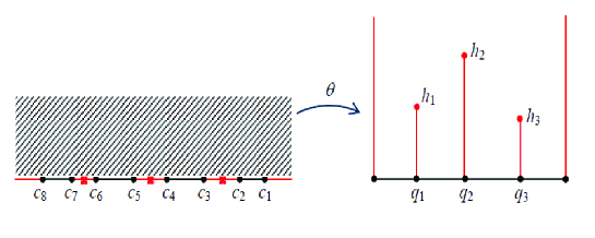
Figure 2: Map $\theta$ for $d=4$, $g=3$; the crosses in $(c_{7},c_{6}),(c_{5},c_{4}),(c_{3},c_{2})$ denote the zeros of $\eta$ and map to $h_{1},h_{2},h_{3}$.

The Chebyshev supports, which is the same as $n$-regular sets, are characterized by $q_{j}$’s being integers (up to a common factor), $j=1,\dots,d-1$ (see e.g. [55]). This corresponds to the conditions $\hat{c}_{1}\in{\mathbb{Q}}^{g},\hat{c}_{2}=0$. In such a case, according to [6], we have

$$\Omega_{\mathbb{A}}(p)=\frac{1}{n}\frac{d{\mathbb{A}}(p)}{{\mathbb{A}}(p)}=\frac{1}{n}\frac{{\mathcal{P}_{n}}^{\prime}(\lambda)d\lambda}{{\mathcal{Q}_{n-2}}(\lambda)\sqrt{\Delta_{2d}(\lambda)}}=\frac{\prod_{j}^{d-1}(\lambda-\hat{\gamma_{j}})d\lambda}{\sqrt{\Delta_{2d}(\lambda)}},$$ (10.6)

where $\mathbb{A}$ is the Akhiezer function and $\Omega_{\mathbb{A}}$ is the differential defined in (2.4), which coincides with $\eta$ in this case, as was pointed out in Section 3. Here $\hat{\gamma_{j}}\in(c_{2j},c_{2j-1})$ are the gap critical points of the polynomial ${\mathcal{P}_{n}}$. The images $(q_{j},h_{j})=\theta(\hat{\gamma_{j}})$ are the tips of the vertical slits at $q_{j}$, $j=1,\dots,d-1$.

Example 2

This is a continuation of Example 1. The image of the map $\theta$ is presented in Fig. 3. Here $d=3,\;g=2$. The values $q_{1}=2/5$ and $q_{2}=4/5$ are obtained from the data of the Chebyshev polynomial $\mathcal{P}_{5}$: its degree being $5$, and the number of critical points in the intervals, namely one critical point in each of the intervals $(c_{6},c_{5})$ and $(c_{4},c_{3})$, and none in the interval $(c_{2},c_{1}).$ The $\theta$-images of the gap critical points of the polynomial $\mathcal{P}_{5},$ those in the gap intervals $(c_{5},c_{4}),(c_{3},c_{2}),$ are the points $(q_{1},h_{1})$ and $(q_{2},h_{2})$. The winding numbers are $(m_{0},m_{1},m_{2})=(5,4,2)$ and the frequencies are $m_{2}/m_{1}=f_{1}=q_{1}=2/5$ and $m_{1}/m_{0}=f_{2}=q_{2}=4/5$.

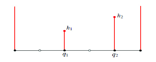
Figure 3: The comb region for $\mathcal{P}_{5}$ from Example 1

We conclude with the following statement about explicit rectification of isoharmonic deformations.

Theorem 5

Consider the map $\theta$ (10.5) corresponding to the Green function of the complement of the union $E$ of $d$ real intervals, from the upper half-plane to the comb region defined by points $q_{j},h_{j}$, $j=1,\dots,d$. Any isoharmonic deformation of $(E^{c},\infty)$ keeps the points $q_{j}$ unchanged, i.e. the base of the comb is invariant under the isoharmonic deformations. The deformation applies only vertically by varying $h_{j}$, the $\theta$-images of the critical points of the Green function, along the vertical rays based at $q_{j}$, for each $j=1,\dots,d-1$.

10.3 The inheritance problem and the injectivity of the frequency map

One of the problems of the 1991 Miklós Schweitzer Mathematical Contest organized by the János Bolyai Mathematical Society in Hungary, with a slight generalization was [58, 59]:

To divide an inheritance, $d>2$ siblings turn to a judge. Secretly however, each of them bribes the judge. What a given sibling inherits depends continuously and monotonically on the bribes: it increases monotonically with respect to the value of their own bribe and decreases monotonically with respect to the value of the bribe of everybody else. Show that if the eldest sibling does not give too much to the judge, then the others can choose their bribes so that the decision will be fair, i.e., each of them gets an equal share.

In [58, 59], this problem, its variations, and more precise formulations were discussed in the framework of the so-called monotone systems: denote by ${\bf t}=(t_{1},\dots,t_{d})$ the set of bribes, with $t_{j}$ being the bribe of the $j$-th sibling and $h_{k}(\bf t)$ denotes the share obtained by the $k$-th sibling with the bribes being equal to $\bf t$. Then these parameters satisfy (i) each $h_{k}$ is a continuous function; (ii) each $h_{k}$ is strictly increasing in $t_{k}$ and strictly decreasing in $t_{j}$ for all $j\neq k$; (iii) the sum is constant: $\sum_{j=1}^{d}h_{j}({\bf t})=1$.

There are various incarnations of the monotone systems, see [58]. Here we are particularly interested in the following situation, see [59]. Using the notation from Section 3, let

$$E=[c_{2d},c_{2d-1}]\cup[c_{2d-2},c_{2d-3}]\cup\dots\cup[c_{2},c_{1}]\,\quad\text{with}\quad c_{2d}<c_{2d-1}<\dots<c_{1}.$$

Assume that each $t_{j}$ is nonnegative and smaller than $\hat{t}=\min_{k}(c_{2k-2}-c_{2k-1})/2,\,k=1,\dots,d-1,$ and

$$E({\bf t})=[c_{2d},c_{2d-1}+t_{d}]\cup[c_{2d-2},c_{2d-3}+t_{d-1}]\cup\dots\cup[c_{2},c_{1}+t_{1}]\,\quad\text{with}\quad c_{2d}<c_{2d-1}<\dots<c_{1}.$$

Then

$$h_{j}({\bf t}):={\mathcal{M}}_{E(\bf t)}[c_{2j},c_{2j-1}+t_{j}],$$

form a monotone system. Given the existence of a trivial solution ${\bf t}={\bf 0}$, the positive answer to the inheritance problem may seem in contradiction with the injectivity of the frequency map defined in (3.3). However, there is no contradiction because in Section 3 (and in the rest of this paper) we assume that one interval remains fixed, which, in the language of the inheritance problem, means that we assume that for one $j\in\{1,2,\dots,d\}$ the corresponding $t_{j}$ is zero. We come to the following:

Proposition 7

If one of the intervals does not participate in the bribing scheme, i.e. if there exists $j$ such that $t_{j}=0$ then the inheritance problem does not have any fair solution, apart from the trivial one when all other intervals also do not participate in the bribing, i.e. when ${\bf t}={\bf 0}$.

Acknowledgements. We thank Patrick Labelle for very helpful discussions concerning the polynomials $L_{l}$ and Jean-Philippe Burelle for his very useful comments upon reading parts of the manuscript. V.D. acknowledges with gratitude the Simons Foundation grant no. 854861 and the support from the University of Texas at Dallas, MISANU, the Serbian Ministry of Education, Science, and Technological Development, the Science Fund of Serbia. V.S. gratefully acknowledges support from the Natural Sciences and Engineering Research Council of Canada through a Discovery grant and from the University of Sherbrooke.

References

- [1]
- [2] N. I. Ahiezer, Lekcii po Teorii Approksimacii, [in Russian], OGIZ, Moscow-Leningrad, 1947, pp. 323.
- [3] N. I. Akhiezer, Elements of the theory of elliptic functions, Translations of Mathematical Monographs, volume 79, American Mathematical Society, Providence, RI, 1990, pp. viii+237.
- [4] G. E. Andrews, The Theory of Partitions, Addison-Weslay, Readings, 1976.
- [5] M. Audin, Courbes algébriques et systèmes intégrables: géodesiques des quadriques, Exposition. Math. 12, 1994, 193–226.
- [6] A. Bogatyrev, Extremal polynomials and Riemann surfaces, Springer Monographs in Mathematics, Springer, Heidelberg, 2012, pp. xxvi+150 pp.
- [7] A. Cayley, Note on the porism of the in-and-circumscribed polygon, Philosophical magazine 6 (1853), 99–102.
- [8] S.-J. Chang, B. Crespi, and K.-J. Shi, Elliptical billiard systems and the full Poncelet theorem in dimensions, J. Math. Phys. 34 (1993), no. 6, 2242–2256.
- [9] Chen, Z, Kuo T-J, Lin, C-S, Wang C-L, Green function, Painlevé VI equation, and Eisenstein series of weight one, J. Differential Geom. Volume 108, Number 2 2018, 185–241.
- [10] G. Darboux, Sur les polygones inscrits et circonscrits á l’ellipsoïde, Bulletin de la Societé philomathique 7 (1870), 92–94.
- [11] G. Darboux, Lecons sur la théorie générale des surfaces et les applications géometriques du calcul infinitésimal, Vol. 2 and 3, Gauthier-Villars, Paris, 1914.
- [12] P. Deift, A. Its, A. Kapaev, X. Zhou, On the algebro-geometric integration of the Schlesinger equations, Commun. Math. Phys. 203 (1999), 613–633.
- [13] V. Dragović, M. Radnović, Geometry of integrable billiards and pencils of quadrics, Journal Math. Pures Appl. 85 (2006), 758–790.
- [14] V. Dragović, M. Radnović, Poncelet porisms and beyond, monograph, Springer-Birkhäuser (2011)
- [15] V. Dragović, M. Radnović, Periodic ellipsoidal billiard trajectories and extremal polynomials, Comm. Math. Physics. 2019, Vol. 372, p. 183-211.
- [16] V. Dragović, M. Radnović, Poncelet polygons and monotonicity of rotation numbers: iso-periodic confocal pencils of conics, hidden traps, and marvels, arXiv: 2103.01215, 2021.
- [17] V. Dragović, V. Shramchenko, Algebro-geometric solutions of the Schlesinger systems and the Poncelet-type polygons in higher dimensions, IMRN, Vol. 2018, No 13, p. 4229–4259 doi:10.1093/imrn/rnx015.
- [18] V. Dragović, V. Shramchenko, Algebro-geometric approach to an Okamoto transformation, the Painlevé VI and Schlesinger equations, Annales Henri Poincaré, 2019, 20, no. 4, 1121–1148.
- [19] V. Dragović, V. Shramchenko, Deformation of the Zolotarev polynomials and Painleve VI equations, Letters in Mathematical Physics, 111, 75 (2021). https://doi.org/10.1007/s11005-021-01415-z.
- [20] V. Dragović, R. Gontsov, V. Shramchenko, Triangular Schlesinger systems and superelliptic curves, Physica D, 2021.
- [21] J. J. Duistermaat, Discrete integrable systems: QRT maps and elliptic surfaces, Springer Monographs in Mathematics, Springer, New York, (2010).
- [22] A. Eremenko, A. Gabrielov, Circular pentagons and real solutions of Painlevé VI equations, Comm. Math. Phys., 355, 1 (2017) 51–95.
- [23] A. Eremenko, P. Yuditskii, Comb functions, Contemporary Mathematics, Vol. 578, 2012.
- [24] J. Fay, Kernel functions, analytic torsion, and moduli spaces, Memoirs of the AMS 96 (1992), no 464.
- [25] R. Fuchs, Über lineare homogene Differentialgleichungen zweiter Ordnung mit drei im Endlichen gelegenen wesentlich singulären Stellen. Math. Ann. 63 (1907), 301–321.
- [26] B. Gambier, Sur les équations différentielles du second ordre et du premier degré dont l’intégrale générale est à points critiques fixes. C. R. Acad. Sci. Paris 142 (1906), 266–269.
- [27] R. Garnier, Sur des équations différentielles du troisième ordre dont l’intégrale générale est uniforme et sur une classe d’équations nouvelles d’ordre supérieur dont l’intégrale générale a ses points critiques fixes, Ann. Sci. École Norm. Sup. 29, no. 3 (1912), 1–126.
- [28] R. Garnier, Solution du problème de Riemann pour les systèmes différentiels linéaires du second ordre, Ann. Sci. École Norm. Sup. 43 (1926), 239–352.
- [29] P. Griffiths, J. Harris, On Cayley’s Explicit Solution to Poncelet’s Porism, Enseignement Mathématique (2), 24, no. 1–2, 31-40 (1978)
- [30] P. G. Grinevich, M. U. Schmidt, Period preserving nonisospectral flows and the moduli space of periodic solutions of soliton equations: The nonlinear Schrödinger equation, Physica D, 87:73–98, 1995.
- [31] N. Hitchin, Twistor spaces, Einstein metrics and isomonodromic deformations, J. Diff. Geom. 3, 52–134 (1995)
- [32] N. Hitchin, Poncelet polygons and the Painlevé equations, Geometry and analysis (Bombay, 1992), 151–185, Tata Inst. Fund. Res., Bombay (1995).
- [33] E. L. Ince, Ordinary differential equations Dover, New York (1956).
- [34] K. Iwasaki, H. Kimura, S. Shimomura, M. Yoshida, From Gauss to Painlevé. A modern theory of special functions, Aspects of Mathematics, Braunschweig (1991).
- [35] A. Kitaev, D. Korotkin, On solutions of the Schlesinger equations in terms of -functions. Internat. Math. Res. Notices (1998), no. 17, 877-905
- [36] A. Kokotov, D. Korotkin, A new hierarchy of integrable systems associated to Hurwitz spaces, Philos. Trans. R. Soc. Lond. Ser. A Math. Phys. Eng. Sci. 366 (2008), no. 1867, 1055–1088.
- [37] D. Korotkin, Solution of matrix Riemann–Hilbert problems with quasi-permutation monodromy matrices, Math. Ann. 329 (2004), 335–369.
- [38] V. V. Kozlov, D. Treshchev, Billiards, Amer. Math. Soc., Providence RI, 1991.
- [39] H. Lebesgue, Les coniques, Gauthier-Villars, Paris, 1942.
- [40] F. Loray, Isomonodromic deformation of Lamé connections, Painlevé VI equation and Okamoto symmetry. Izvestiya: Mathematics 80 1 (2016) p.113–166.
- [41] Yu. Manin, Sixth Painlevé equation, universal elliptic curve, and mirror of P2. Am. Math. Soc. Trans. Ser. 2(186), 131-151 (1998)
- [42] V. A. Marchenko, I. V. Ostrovski, A characterization of the spectrum of the Hill operator. Math. USSR Sb. 97(1975), no. 4, 540–606, in Russian.
- [43] A. Martinez-Finkelshtein, B. Simanek, B. Simon, Poncelet’s Theorem, Paraorthogonal Polynomials and the Numerical Range of Compressed Multiplication Operators, Adv. Math, 2019
- [44] H. P. McKean, Integrable systems and algebraic curves, in Global Analysis, Ed. M. Grimela J. E. Marsden, LNM Vol. 755, 1979, p. 83–200.
- [45] J. Moser, A. Veselov, Discrete versions of some classical integrable systems and factorization of matrix polynomials, Comm. Math. Phys. 139 (1991), no. 2, 217–243.
- [46] M. S. Narasimhan, G. Trautmann, Compactification of and Poncelet pairs of conics, Pacific J. Math. 145 (1990), 255-365.
- [47] K. Okamoto, Studies on the Painlevé equations. I. Sixth Painlevé equation . Ann. Mat. Pura Appl. (4) 146 1987, 337 – 381.
- [48] F. Peherstorfer, K. Schiefermayr, Description of extremal polynomials on several intervals and their computation, I, II, Acta Math. Hungar. 83 (1999), no. 1-2, 27–58, 59–83.
- [49] E. Picard, Mémoire sur la théorie des fonctions algébriques de deux variables, Journal de Liouville 5 1889, 135–319.
- [50] R. Ramirez-Ros, On Cayley conditions for billiards inside ellipsoids, Nonlinearity 27 (2014), no. 5, 1003–1028.
- [51] L. Schlesinger, Über eine Klasse von Differentialsystemen beliebiger Ordnung mit festen kritischen Punkten, J. Reine Angew. Math. 141 (1912), 96–145.
- [52] B. Simon, Szegö’s Theorem and Its Descendants, Princeton University Press, 2011.
- [53] B. Simon, Harmonic Analysis. A Comprehensive Course in Analysis, Part 3, AMS, 2015.
- [54] B. Simon, Operator Theory. A Comprehensive Course in Analysis, Part 4, AMS, 2015.
- [55] M. L. Sodin, P. M. Yuditskii, Functions that deviate least from zero on closed subsets of the real axis, Algebra i Analiz 4 (1992), no. 2, 1–61 (Russian, with Russian summary); English transl., St. Petersburg Math. J. 4 (1993), no. 2, 201–249.
- [56] G. Springer, Introduction to Riemann Surfaces, AMS Chelsea Publishing, 1957, p. 309.
- [57] V.Totik, Polynomial inverse images and polynomial inequalities, Acta Math. 187(2001)139–160.
- [58] V. Totik, The inheritance problem and monotone systems, Austral. Math. Soc. Gaz. 33 (2006), no. 2, 122–130.
- [59] V. Totik, Chebyshev constants and the inheritance problem, J. Approx. Theory 160 (2009), no. 1-2, 187–201.
- [60] S. Tabachnikov, Geometry and billiards, Student Mathematical Library, vol. 30, American Mathematical Society, Providence, RI, 2005.
- [61] G. Teschl, Jacobi Operators and Completely Integrable Nonlinear Lattices, Mathematical Surveys and Monographs Volume 72, AMS, 2000.
- [62] J. L. Walsh, The Location of Critical Points of Analytic and Harmonic Functions, AMS, Colloquium Publications, Vol. 34, 1950.
- [63] H. Widom, Extremal polynomials associated with a system of curves in the complex plane, Adv. Math. 3, (1969), 127–232.