Learning Linear Models Using Distributed Iterative Hessian Sketching

Abstract

This work considers the problem of learning the Markov parameters of a linear system from observed data. Recent non-asymptotic system identification results have characterized the sample complexity of this problem in the single and multi-rollout setting. In both instances, the number of samples required in order to obtain acceptable estimates can produce optimization problems with an intractably large number of decision variables for a second-order algorithm. We show that a randomized and distributed Newton algorithm based on Hessian-sketching can produce $\epsilon$-optimal solutions and converges geometrically. Moreover, the algorithm is trivially parallelizable. Our results hold for a variety of sketching matrices and we illustrate the theory with numerical examples.

1 Introduction

Obtaining a dynamic model of a system or process is fundamental to most of science and engineering. As the systems we study become increasingly complex, data-driven modeling has become the de facto framework for obtaining accurate models (Brunton and Kutz, 2019). Fortunately, as systems become more interconnected and sensors become smaller and cheaper, there is no shortage of data to work with. Indeed, the volume of data available can overwhelm the (often limited) computational resources at our disposal, forcing us to consider data versus resource trade-offs (Chandrasekaran and Jordan, 2013).

There has recently been considerable interest in applying machine learning techniques to the problem of controlling a dynamical system. Two paradigms have emerged; model-based control, in which a model is first learnt from data and then a classical controller is synthesized from the model. In the model-free setting the control action is learnt directly from data without ever constructing an explicit model, see for example Fazel et al. (2018). Our work is motivated by two observations; i) the asymptotic sample complexity of a model-based solution outperforms that of a model-free Least-Squares Temporal Difference Learning (Boyan, 1999) approach  Tu and Recht (2019); ii) the recent body of work characterizing the sample complexity of learning linear system models from data, shows that for systems with a large number of inputs and outputs, the resulting optimization problems are intractable as they require a large number of rollouts or long trajectory horizon lengths in order to produce accurate estimates Oymak and Ozay (2019); Zheng and Li (2020); Tsiamis and Pappas (2019); Dean et al. (2020). The goal of this work is to construct and solve approximations of these optimization problems that are consistent with the sample complexity results, provide provably good solutions, and do so in an algorithmically tractable manner. Our approach is based on the concept of “sketching” (Drineas and Mahoney, 2016). Broadly speaking, a “sketch” is an approximation of a large matrix by a smaller or more “simple” matrix. For a sketch to be useful, it must retain certain properties of the original matrix that allow it to be used for computation in place of the original. What is perhaps surprising, is that randomization is the enabling force used to construct sketches (Woodruff, 2014; Martinsson and Tropp, 2020; Mahoney, 2011). Moreover, numerical linear algebra routines based on randomization (and sketching) can outperform their deterministic counterparts (Avron et al., 2010), and are more suited to distributed computing architectures.

1.1 Problem Setting

Notation: Given a matrix $A\in\mathbb{R}^{m\times n},$ we use $\lVert A\rVert_{F}$ to denote its Frobenius norm. The multivariate normal distribution with mean $\mu$ and covariance matrix $\Sigma$ is denoted by $\mathcal{N}\left(\mu,\Sigma\right).$ For two functions $f(x)$ and $g(x)$, the notation $f(x)=O(g(x))$ or $f(x)\lesssim g(x)$ implies that there exists a universal constant $C<\infty$ satisfying $f(x)\leq Cg(x)$. For an event $\mathcal{X}$, $\mathbb{P}(\mathcal{X})$ refers to its probability of occurrence.

Let us assume that we have a stable and minimal, linear time-invariant (LTI) system given by

$$x_{t+1} =Ax_{t}+Bu_{t}+w_{t},\quad x_{0}=0$$ (1)

$$y_{t} =Cx_{t}+Du_{t}+v_{t}$$

where $x_{t}\in\mathbb{R}^{n},~{}y_{t}\in\mathbb{R}^{p},$ and $u_{t}\in\mathbb{R}^{m}$ denote the system state, output, and input at time $t$, respectively, and $w_{t}\in\mathbb{R}^{n},v_{t}\in\mathbb{R}^{p}$ denote the process and measurement noises. We assume that ${u}_{t}\sim\mathcal{N}\left(0,\sigma_{u}^{2}{I}_{m}\right),{w}_{t}\sim\mathcal{N}\left(0,\sigma_{w}^{2}{I}_{n}\right)$, and ${v}_{t}\sim\mathcal{N}\left(0,\sigma_{v}^{2}{I}_{p}\right).$ Our goal is to learn the system parameters $A,B,C$ and $D$ from a single input and output trajectory $\{y_{t},u_{t}\}^{\bar{N}}_{t=1}$. We are particularly interested in the scenario of “large” $m$ and $p$, and where sample complexity results show that $\bar{N}$ must be huge in order to achieve accurate estimates. In this parameter regime many optimization methods are intractable and even routine matrix factorizations become problematic.

To achieve this goal, we begin by estimating the first $T$ Markov parameters $G$, which are defined as:

$$G=\left[\begin{array}[]{ccccc}D&CB&CAB&\cdots&CA^{T-2}B\end{array}\right]\in\mathbb{R}^{p\times mT}.$$

Then system matrices $A,B,C$ and $D$ can be realized via the Ho-Kalman algorithm (Ho and Kálmán (1966)). In recent work we applied similar ideas based on randomized methods to implement a stochastic version of the Ho-Kalman algorithm suitable for masive-scale problems (Wang and Anderson, 2021). We thus narrow our attention in this work to the task of providing an estimate $\hat{G}$ of $G$.

As described in Oymak and Ozay (2019), we first generate a trajectory of length $\bar{N}$. The trajectory is then spliced and written into two matrices corresponding to the control and output signal. Define $\bar{N}=T+N-1$ with $N\geq 1$, let

$$Y=\left[\begin{array}[]{cccc}y_{T}&y_{T+1}&\cdots&y_{\bar{N}}\end{array}\right]^{T}\in\mathbb{R}^{N\times p}\text{~{}~{}~{} and~{}~{}~{} }U=\left[\begin{array}[]{cccc}\bar{u}_{T}&\bar{u}_{T+1}&\cdots&\bar{u}_{\bar{N}}\end{array}\right]^{T}\in\mathbb{R}^{N\times mT},$$

with $\bar{u}_{i}$ denoting $\bar{u}_{t}=\left[u_{i}^{T},u_{i-1}^{T},\cdots,u_{i-T+1}^{T}\right]^{T}\in\mathbb{R}^{mT}$. Then the Markov parameters $G$ can be learned by solving the following unconstrained least-squares problem:

$$X^{\mathrm{LS}}=\underset{{X}\in R^{mT\times p}}{\operatorname{argmin}}\|{Y}-{U}X\|_{F}^{2}.$$ (2)

The estimate is obtained from $\hat{G}=(X^{\mathrm{LS}})^{T}$. Oymak and Ozay (2019) provided the following non-asymptotic sample complexity bound:

$$\|\hat{G}-G\|_{F}\leq\frac{\left(\sigma_{v}+\sigma_{e}\right)\sqrt{p}+\sigma_{w}\|F\|_{2}}{\sigma_{u}}\sqrt{\frac{Tq\log^{2}(Tq)\log^{2}(Nq)}{N}}$$ (3)

holds with high probability, as long as $N\gtrsim Tq\log^{2}(Tq)\log^{2}(Nq)$, where $q=m+p+n$ is the aggregated system dimension. The matrix $F=\left[\begin{array}[]{ccccc}0&C&CA&\cdots&CA^{T-2}\end{array}\right]\in\mathbb{R}^{p\times Tn}$ is the concatenated matrix and $\sigma_{e}^{2}$ is the variance of the linearly transformed state at time $i-T+1.$ Interested readers can refer to Oymak and Ozay (2019) for more details.

1.2 Motivation

From (3), it is clear that increasing the sample size $N$ can make the estimated Markov parameters more reliable. To achieve better identification performance, $N$ needs to be large, i.e., $N\gg Tq\log^{2}(Tq)\log^{2}(Nq)$. In other words, we need to solve the least square problem described by Eq 2 with $N\gg mT$ (The number of rows is significantly larger than the number of columns).

To solve problem (2), Oymak and Ozay (2019); Zheng and Li (2020); Tsiamis and Pappas (2019); Dean et al. (2020) adopted the pseudo-inverse method. However, the complexity of computing the pseudo-inverse method requires $O((mT)^{2}N)$ flops, which is costly for large systems. Moreover, for truly huge-scale systems, the memory cost for storing the sample trajectories ($U$ and $Y$) will likely exceed the storage capacity of a single machine. Therefore, there is a strong desire to put forward a tractable algorithm, which can take advantage of modern distributed computing architectures. In this paper, we consider the setting where there are $r$ worker machines operating independently in parallel and a single central node that computes the averaged solution. No communication between workers is permitted as it is likely that communication time dominates local computation time in the distributed algorithms. We only allow the communications between worker and the central node. Overall, we aim to provide a communication $\&$ computation-efficient algorithm to solve the large-scale system identification problems defined by Eq (2).

1.3 Related work

System identification: Estimating a linear dynamical system from input/output observations has a long history, which can date back to the 1960s. Prior to the 2000s, most identification methods for linear systems either focus on the prediction error approach Ljung (1999) or subspace methods Van Overschee and De Moor (2012); Verhaegen and Verdult (2007). In contrast, with the advances in high-dimensional statistics Vershynin (2018), contemporary research shifts from asymptotic analysis with infinite data assumptions to finite time analysis and finite data rates. Over the past several years, there have been significant advances in studying the finite sample properties, when the system state is fully observed Simchowitz et al. (2018); Sarkar and Rakhlin (2019); Faradonbeh et al. (2018). When the system is partially observed, we can find the finite sample analysis in Oymak and Ozay (2019); Sarkar et al. (2019); Simchowitz et al. (2019); Tsiamis and Pappas (2019); Lee and Lamperski (2020); Zheng and Li (2020); Lee (2020); Lale et al. (2020); Kozdoba et al. (2019). However, there are only a few papers Sznaier (2020); Reyhanian and Haupt (2021) that consider the computational complexity and memory issues of system identification, which become prohibitively large and incompatible with on-board resources when system dimension increases. There is thus a great need to provide scalable algorithms which can efficiently solve the system identification problem.

Distributed optimization: In recent years, a lot of effort has been devoted to designing distributed first-order methods (Mahajan et al., 2013; Shamir and Srebro, 2014; Lee et al., 2017; Fercoq and Richtárik, 2016; Liu et al., 2014; Necoara and Clipici, 2016; Richtárik and Takáč, 2016; Liu et al., 2020), which only rely on gradient information of the objective function. However, first-order methods suffer from: (i) a dependence on a suitably defined condition number; (ii) spending more time on communication than on computation. To overcome these drawbacks, second-order methods have received more attention recently, since they enjoy superior convergence rates which are independent of the condition number and thereby require fewer rounds of communication to achieve high accuracy solutions.

The trade-off is that most second-order algorithms based on Newton’s method require forming and then computing the inverse of Hessian matrix at each iteration. For large problem instances this is overly time consuming. Quasi-Newton methods have been developed that approximate the Hessian, however the convergence analysis is weaker than the full method (Dennis and Moré, 1977). There are a lots of works in the field of distributed second order optimization such as Zhang and Lin (2015), Smith et al. (2018), Wang et al. (2017b) and Crane and Roosta (2019). In this work we take an alternative approach that retains the linear-quadratic convergence of Newton’s method (Pilanci and Wainwright, 2017) and adapt it to the distributed, which was first introduced in Bartan and Pilanci (2020), but communication efficient setting. The key idea is to “sketch” the Hessian at each iteration.

1.4 Contribution

In this paper, we use the distributed iterative Hessian sketch algorithm (DIHS) which was introduced by Bartan and Pilanci (2020) to solve the large-scale system identification problems in a more scalable manner. Specifically, our contributions are:

• We give a new proof and a different convergence rate from Bartan and Pilanci (2020); Wang et al. (2017b) for the DIHS algorithm.

• We provide a convergence guarantees for the DIHS algorithm with various sketching schemes on the matrix least square problems, not limited to Gaussian sketches mentioned in Bartan and Pilanci (2020).

• We show that DIHS algorithm is consistent with the non-asymptotic sample complexity bound $O(\frac{1}{\sqrt{N}})$ for learning the Markov parameters.

2 Background

Sketching has become a popular method for scientific computing workflows that deal with massive data sets; or more precisely, massive matrices (Drineas and Mahoney, 2016). We develop an iterative, distributed sketching algorithm for solving system identification problems that are formulated as least-squares problems of the form (2). Consider the overdetermined least-squares problem with problem data $A\in\mathbb{R}^{n\times d}$, $b\in\mathbb{R}^{n}$, where $n\gg d$:

$$\underset{{x}\in\mathbb{R}^{d}}{\operatorname{minimize}}~{}\|Ax-b\|_{2}^{2},$$

and let $x^{\star}$ denote an optimal solution. Assuming $A$ is dense and has no discernible structure, factorization-based approaches solve the problem in $O(nd^{2})$ arithmetic operations. The sketch-and-solve approach constructs a matrix $S$ of dimension $m\times n$ (where $m\ll n$) and solves

$$x^{\sharp}\in\underset{{x}\in\mathbb{R}^{d}}{\operatorname{argmin}}~{}\|S(Ax-b)\|_{2}^{2},$$

instead of the original problem. The driving idea is that if $m$ is small, then solving this problem is easier than solving the original problem. Amazingly, letting $S$ be a random matrix chosen from an appropriate distribution (to be defined later) will suffice. The matrix $SA$ is called the the sketch of $A$ and $S$ is the sketching matrix or embedding matrix. If $S$ is chosen as a subspace embedding of $\text{Range}([A~{}b])$ then the action of $S$ preserves geometry and one can show that the residuals satisfy $\|Ax^{\sharp}-b\|_{2}\leq(1+\epsilon)\|Ax^{\star}-b\|_{2}$, with high probability, where $\epsilon>0$ is the distortion of the embedding. In practice, even when the residuals are close, there is no guarantee that $\|x^{\sharp}-x^{\star}\|_{2}$ will be small. This problem will be alleviated by iterative-sketching methods derived by Pilanci and Wainwright (2016) described later. However, the sketch-and solve framework highlights several important points: How do we choose the random embedding (the matrix $S$)? How is the projection dimension $m$ chosen? Indeed, for the bound above to hold we require $m\sim d\log(d)/\epsilon^{2}$ (Sarlos, 2006). A geometric-type bound by Pilanci and Wainwright (2015) showed that when entries of $S$ are sub-Gaussian, one requires $m\geq\frac{c}{\delta^{2}}\mathcal{W}(A\mathcal{K})$ to obtain similar quality bounds in residual, where $\mathcal{W}(A\mathcal{K})$ is the Gaussian width (Vershynin, 2018) of the cone $A\mathcal{K}$. Clearly there is tension between making $m$ small (improved computation) and obtaining an accurate solution.

When $S$ is selected to be a dense matrix, the cost of forming $SA$ is $O(mnd)$ and no computational saving is achieved. However, there exist families of randomized matrices that admit a fast matrix-vector multiply which reduce the cost of forming the product to $O(nd\log(m))$ thus providing significant savings. In addition to the dense sub-Gaussian case, we will consider of randomized embeddings defined by; randomized orthogonal systems (ROS) Ailon and Chazelle (2009), Sparse Johnson-Lindenstrauss Transforms (SJLTs) (Kane and Nelson, 2014), and uniform sampling.

3 Distributed Iterative Hessian Sketch

Consider the optimization problem (2). Applying Newton’s method with a variable step-size $\alpha_{t}$, produces a sequence of iterates of the form:

$$X_{t+1}=X_{t}-\alpha_{t}(U^{T}U)^{-1}U^{T}(UX_{t}-Y),\quad t=1,2,\dots$$ (4)

where the Hessian is given by $U^{T}U$ and the gradient by $U^{T}(UX_{t}-Y)$ c.f., (Boyd et al., 2004). Given that the columns of $U$ are made up from the control input which we assume to be random Gaussian variables, $U$ will be a dense matrix. Under the assumption that $(N,m,T)$ are large forming the Hessian and the gradient will grind the Newton iterates to a halt.

Instead of computing the iterate (4) exactly, Pilanci and Wainwright (2016) introduced the iterative Hessian sketch (IHS) to approximate the Hessian. The explicit update rule is given by:

$$X_{t+1}=X_{t}-\alpha_{t}(U^{T}S_{t}^{T}S_{t}U)^{-1}U^{T}(UX_{t}-Y),$$ (5)

where $S_{t}\in\mathbb{R}^{s\times N}(s\ll N)$ denotes the embedding matrix at the $t^{\text{th}}$ iteration. The matrix $U^{T}S^{T}SU$ is called the the “sketched Hessian”. We will now introduce some specific classes of sketching matrices.

Definition 3.1.

A random variable $x$ such that $\mathbb{E}x=0$ is said to be sub-Gaussian with variance proxy $\sigma$, if its moment generating function satisfies

$$\mathbb{E}\{\exp(\lambda x)\}\leq\exp\left({\frac{\sigma^{2}\lambda^{2}}{2}}\right).$$

An equivalent characterization of a sub-Gaussian random variable obtained from Markov’s inequality is that $\mathbb{P}(|x|\geq\lambda)\leq 2\exp(-t^{2}/4)$, where $t=2\lambda$ and $\sigma=1$. We write $x\in\mathtt{subG}(\sigma^{2})$ to denote that $x$ is sub-Gaussian. Note that this notation is not precise in the sense that $\mathtt{subG}(\sigma^{2})$ denotes a family of distributions. The particular choice of distribution will be clear from context. We consider the following families of random sketching matrices from which we draw $S\in\mathbb{R}^{s\times N}$:

• Sub-Gaussian: Each element of $S$ is drawn from a specific sub-Gaussian distribution, i.e., $S_{ij}\stackrel{{\scriptstyle\mathclap{\text{\scriptsize{ \tiny i.i.d.}}}}}{{\sim}}\mathtt{subG}(\sigma^{2})$ where the particular distribution is fixed for all entries. Examples of distributions that satisfy Definition 3.1 include Gaussian, Bernoulli, and more generally, any bounded distribution. Note that the sub-class of Gaussian sketch matrices are almost surely dense, thus they are often useful for proving results, and less useful for computation.

• Uniform: Let $\{p_{i}\}_{i=1}^{N}$ denote the uniform distribution over $1,\ldots,N$. Then the uniform sketch samples the rows $s$ times (with replacement). The $j^{\text{th}}$ row of $S$ is $s_{j}^{T}=e_{j}/\sqrt{p_{j}}$ with probability $p_{j}$, where $e_{j}$ is the $j^{\text{th}}$ standard basis vector. Other weights (probability distributions ) have been studied, however we do not pursue these here.

• Random Orthogonal System (ROS)-based Sketch: This sketching matrix is based on a unitary trigonometric transform $F\in\mathbb{F}^{N\times N}$ (defined in appendix A). As our least-squares problem is defined over the reals we restrict our attention to real transforms, and in particular the Walsh-Hadamard Transform. The matrix $S$ is then formed according to

  $$S=\sqrt{\frac{N}{s}}RFE,$$

  where $E=\mathrm{diag}(\nu_{1},\dots,\nu_{N})$ with $\nu_{i}$ drawn uniformly at random from $\{+1,-1\}$. The matrix $R$ is a $s\times N$ uniform sketching matrix defined above. The structure of an ROS matrix allows for a fast matrix-vector multiply.

• Sparse Johnson-Lindenstrauss Transform (SJLT)-based Sketches. SJLT sketching matrices are another structured random matrix family that offer fast matrix-vector multiplication and are particularly suitable when the matrix to be sketched is sparse. Several constrictions exist, we follow that of (Kane and Nelson, 2014). Each column of $S$ has exactly $l$ non-zero entries at randomly chosen coordinates. The non-zero entries are chosen uniformly from $\{+1/\sqrt{l},-1/\sqrt{l}\}$. SJLT matrices also belong to the class of sub-Gaussian sketching matrices.

Loosely speaking, ROS and SJLTs when applied to a vector attempt to evenly mix all the coordinates and then randomly sample to obtain a lower dimensional vector with norm proportional to the original vector. In contrast, uniform sampling simply selects a subset of rows of $A$ chosen uniformly at random. A dense sub-Gaussian sketching matrix extends uniform sampling by linearly weighting the entries of each row.

Compared to $O((mT)^{2}N)$ flops given by pseudo-inverse method, IHS with ROS or SJLT sketches takes $O((NmT\log(mT))\log(1/\epsilon))$ flops, which is linear in $NmT$, to obtain an $\epsilon$-accurate solution. Obviously, IHS has significantly lower complexity than direct method since we assume $N\gg mT$.

Remark 3.2.

IHS can also deal with the least square problem with $N\ll mT.$ In this case, we just need to sketch the column-space instead of the row-space. The constrained case is also easily handled.

Just as with the Gaussian Newton Sketch, which produces unbiased estimates of the exact Newton step, many sketching matrices provide near-unbiased estimates of the Newton step (Derezinski et al., 2021). This property is very important in distributed setting, where we can compute the iterate (5) multiple times in parallel. Averageing schemes can then be employed to achieve better estimation performance (Dereziński and Mahoney, 2019; Wang et al., 2017b, a). Using this idea, Bartan and Pilanci (2020) introduced the Distributed-IHS (DIHS) algorithm, which is described by Algorithm 1.

Algorithm 1 Distributed Iterative Hessian Sketch (DIHS)

1:Inputs: Input matrix $U\in\mathbb{R}^{N\times mT}$, output matrix $Y\in\mathbb{R}^{N\times p}$, sketching size $s\ll N$.

2:Initialize: Initial iterate $X_{0}\in\mathbb{R}^{mT\times p}$

3:for $t=0,1,\cdots,M-1$ do

4: Central node: broadcasts $X_{t}$

5: for worker $i=1,2,\cdots,r$ do in parallel

6:  Generate a sketching matrix $S_{i}^{t}\in\mathbb{R}^{s\times N}$

7:  Compute gradient $g_{t}=U^{T}\left(UX_{t}-Y\right)$.

8:  $X_{i}^{t}=\underset{X}{\arg\min}\Big{\{}\frac{1}{2s}\lVert S_{i}^{t}U(X-X_{t})\rVert_{2}^{2}+\langle g_{t},X\rangle\Big{\}}$

9:  Send $X_{i}^{t}$ to the central node

10: end for

11: Central node: Update $X_{t+1}=\frac{1}{r}\sum_{i=1}^{r}X_{i}^{t}$

12:end for

At the $t^{\mathrm{th}}$ iteration of Algorithm 1, each worker $i$ only has a small sketch of the full data set and computes the sketched version of Hessian matrix $U^{T}(S_{i}^{t})^{T}S_{i}^{t}U$ and then computes the local update direction using the sketched Hessian. They then send the updated states to the central node. The central node averages all the states to update the new iteration $X_{t+1}$ and then broadcasts $X_{t+1}$ to all the workers. Using Algorithm 1, the communication complexity decreases from $O((mT)^{2})$ to $O(mT)$ at each iteration since we don’t broadcast the Hessian to each worker, and only communicate the update direction.

Remark 3.3.

Note that the size of the sketching matrix can be different for each worker, i.e., $s\rightarrow s_{i}$ in line 6. This is particulary useful as it allows for the use of a heterogenous set of worker machines, each with their own resource profile.

3.1 Convergence Analysis

We are now ready to state the main results of this work; the convergence analysis of the DIHS algorithm in terms of the approximation error and the estimation quality.

Theorem 3.4.

Fix $\rho\in(0,1/2)$. If the number of rollouts satisfies $N\geq cTm\log^{2}(2Tm)\log^{2}(2\bar{N}m)$ and if

• $S_{i}^{t}$ is a sub-Gaussian sketching matrix with a sketching size $s\geq\frac{c_{0}}{\rho^{2}}mT,$ with probability at least $1-(2\bar{N}m)^{-\log^{2}(2Tm)\log(2\bar{N}m)}-c_{1}rte^{-c_{2}s\rho^{2}}$,

or,

• $S_{i}^{t}$ is a randomized orthogonal system (ROS) sketching matrix with a sketching size $s\geq\frac{c_{0}\log^{4}(mTp)}{\rho^{2}}mT,$ with probability at least $1-(2\bar{N}m)^{-\log^{2}(2Tm)\log(2\bar{N}m)}-c_{1}rte^{-c_{2}\frac{s\rho^{2}}{\log^{4}(mTp)}}$,

then, the output $X_{t}$ given by the DIHS algorithm at the $t^{\mathrm{th}}$ iteration satisfies

$$\lVert X_{t}-X^{\mathrm{LS}}\rVert_{F}\leq 2\Big{(}\frac{\rho}{\sqrt{r}}\Big{)}^{t}\lVert X^{\mathrm{LS}}\rVert_{F},$$

where $X^{\mathrm{LS}}$ denotes the least-squares solution to problem (2), and $c,c_{0},c_{1}$ and $c_{2}$ are absolute constants.

Proof 3.5.

See appendix B for this and subsequent proofs.

Remark 3.6.

The DIHS algorithm converges geometrically to the least-squares solution of (2). The linear convergence rate is $\frac{\rho}{\sqrt{r}}$, which decreases when number of workers $r$ increases. If we apply the DIHS algorithm with $O(\frac{\log(1/\epsilon)}{\log(\sqrt{r}/\rho)})$ iterations and choose the sketching matrices to satisfy the requirement of Theorem 3.4, then the output which we denote by $\hat{X}$ satisfies:

$$\frac{\lVert\hat{X}-X^{\mathrm{LS}}\rVert_{F}}{\lVert X^{\mathrm{LS}}\rVert_{F}}\leq\epsilon$$

with high probability.

Next, we quantify the approximation quality in terms of the distance between the DIHS solution and the ground-truth Markov parameters $G$ in the following theorem.

Theorem 3.7.

Frame the hypotheses of Theorem 3.4. For all $t\geq 1$, the output $X_{t}$ given by the DIHS algorithm satisfies:

$$\lVert X_{t}-G^{T}\rVert_{F}\leq 2\Big{(}\frac{\rho}{\sqrt{r}}\Big{)}^{t}\lVert X^{\mathrm{LS}}\rVert_{F}+\frac{\left(\sigma_{v}+\sigma_{e}\right)\sqrt{p}+\sigma_{w}\|F\|_{2}}{\sigma_{u}}\sqrt{\frac{Tq\log^{2}(Tq)\log^{2}(Nq)}{N}}$$ (6)

with high probability.

Remark 3.8.

Note that the first term of the RHS of (6) linearly converges to $0$ when $t\rightarrow\infty.$ Therefore, the estimation error $\lVert X_{t}-G^{T}\rVert_{F}$ given by the DIHS algorithm still maintains the $O(\frac{1}{\sqrt{N}})$ sample complexity when the number of iterations $t$ becomes large.

4 Numerical Simulations

We now demonstrate the performance of the DIHS algorithm on three randomly generated large-scale dynamic systems described by (1). For each system, we choose the parameters $(n,m,p,N,T)$ as shown in the caption of Figures 1–3. To ensure a fair comparison, we fix a constant sketch dimension for all workers. Recall that theoretically this is unnecessary. We introduce two new sketching matrices. Rademacher sketches are defined such that each entry of $S$ is $\frac{1}{\sqrt{s}}$ with probability $1/2$ and $-\frac{1}{\sqrt{s}}$ otherwise. A two-stage uniform+SJLT sketch is produced from $S(S_{1}U)$ where $S$ is an SJLT sketching matrix with $s$ rows and $S_{1}$ is a uniform sketchimg matrix with $s_{1}$ rows.

We generate the system matrices $(A,B,C,D)$ through a uniform distribution over a range of integers as follows; entries of the matrix $A$ with random integers from $1$ to $5$, and matrices $B,C,D$ with random integers from $-2$ to $2$. Then, we re-scale the matrix $A$ to make it Schur-stable, i.e., $\lvert\lambda_{\mathrm{max}}(A)\rvert<1$. The standard deviations of the process and measurement noises are chosen to be $\sigma_{w}=0.1$ and $\sigma_{v}=0.1$. We fix the input variance at $\sigma_{u}=1$.

The left plot in each figure shows the normalized difference between the estimated solution at each iteration and the optimal least square solution $\|X^{\mathrm{LS}}\|$, (i.e. $\frac{\lVert X_{t}-X^{\mathrm{LS}}\rVert_{F}}{\lVert X^{\mathrm{LS}}\rVert_{F}}$) versus time (seconds) for the DIHS algorithm. In each system, we tested the performance of DIHS algorithm using the uniform and SJLT sketch with $r=5$ and $r=20$ worker machines. The stopping criterion is that the distance between two consequent outputs (i.e. $\lVert X_{t+1}-X_{t}\rVert_{F}$) is less than $10^{-3}$. As predicted by the theoretical analysis, no matter what sketching matrix we use in the DIHS algorithm, the convergence rate decays as the number of workers $r$ increases. Compared to SJLT sketches, it seems that uniform sketching matrices could speed up the convergence throughout these three system identification examples. We note that in terms of computation speed, the uniform sketches should be fast as they require fewer arithmetic operations to apply and less time to construct than every other sketch type.

The middle plot of each figure illustrates the relative error between the estimated solution at the $t^{\mathrm{th}}$ iteration and the optimal least square solution (i.e. $\frac{\lVert X_{t}-X^{\mathrm{LS}}\rVert_{F}}{\lVert X^{\mathrm{LS}}\rVert_{F}}$) against iteration for the DIHS algorithm with different sketching matrices for a fixed number of workers: $r=15.$ Finally, the third column shows the relative error between the estimated solution and true Markov parameters (i.e. $\frac{\lVert X_{t}-G^{T}\rVert_{F}}{\lVert G\rVert_{F}}$) versus iteration with $15$ workers. From the figures, we can easily observe that DIHS algorithm with all these four sketching matrices converges geometrically to the least square solution, which is consistent with the analysis derived from Theorem 3.4. For all sketching matrices we tested, DIHS algorithm can sucessfully learn the true Markov parameter $G$, which is stated in Theorem 3.7. The performance of different sketching matrices depends on the choice of sketching size $s$ and $s_{1}$.

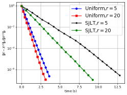
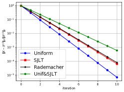
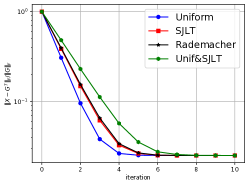
Figure 1: $(n,m,p,N,T)=(80,60,70,29971,30)$, $s=7200,s_{1}=14400$. The dimension of matrix $U$ is $(29971,1800)$ and matrix $Y$ is $(29971,70)$

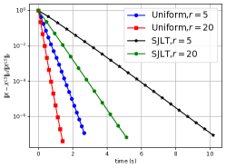
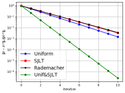
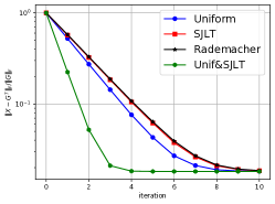
Figure 2: $(n,m,p,N,T)=(100,80,70,49981,20)$, $s=4800,s_{1}=7200$. The dimension of matrix $U$ is $(49981,1600)$ and matrix $Y$ is $(49981,70)$

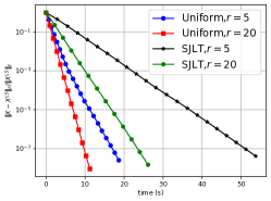
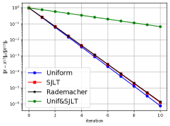
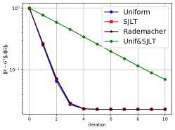
Figure 3: $(n,m,p,N,T)=(200,150,100,59981,20)$, $s=6000,s_{1}=7200$. The dimension of matrix $U$ is $(59981,3000)$ and matrix $Y$ is $(59981,100)$

5 Conclusion

We have demonstrated that a randomized version of Newton’s algorithm can solve large-scale system identification problems and is consistent with recent state-of-the art sample complexity results. Geometric convergence was proven for all the standard sketching matrices and the dimension-dependence of the sketching matrix was also derived. Future work will involve benchmarking this second-order method against distributed first-order methods such as accelerated stochastic gradient descent. We are currently integrating this work with our previous results which uses a randomized SVD to produce a system realization (Wang and Anderson, 2021), with the goal of producing end-to-end bounds.

HW is generously funded by a Wei family fellowship and the Columbia Data Science Institute. We also acknowledge funding from the DoE under grant DE-SC0022234.

Appendix A Walsh-Hadamard Transform

The Walsh-Hadamard transform can be thought of as a generalized Fourier transform built from Hadamard matrices. A Hadamard matrix (Hedayat and Wallis, 1978) is an $n\times n$ matrix with mutually orthogonal columns whose elements take values $\pm 1$. As a result, for any Hadamard matrix $H\in\mathbb{R}^{n\times n}$, we have $H^{T}H=nI$. A recursive construction is a follows: define $H_{0}=1$, then

$$H_{m}=\frac{1}{\sqrt{2}}\left[\begin{array}[]{cc}H_{m-1}&H_{m-1}\\ H_{m-1}&-H_{m-1}\end{array}\right].$$

To apply the Walsh-Hadamard transform to matrices that are not of compatible row dimension we simply pad with zeros.

Appendix B Proofs and auxiliary results

In this section, we prove the main results: Theorem 3.4 and 3.7. We leverage the proof technique from Pilanci and Wainwright (2016). However the results need to be adapted to target the matrix least-squares problem and to account for the distributed problem setting.

We use matrix $X\in\mathbb{R}^{mT\times p}$ to denote the possible descent matrix and vector $x\in\mathbb{R}^{p}$ to denote any column vector in the possible descent matrix $X$. Here we assume a more general formulation where we append the convex constraint $X\in\mathcal{C}$ to Eq (2). The set of possible descent directions $\left\{x-x^{\mathrm{LS}}\mid x\in\mathcal{C}\right\}$ plays an important role in controlling the error w.r.t. the least square solution $X^{\mathrm{LS}}$. The affinely transformed tangent cone is defined as

$$\mathcal{K}^{\mathrm{LS}}=\left\{v\in\mathbb{R}^{N}\mid v=tU\left(x-x^{\mathrm{LS}}\right)\quad\right.\text{for some}\ t\geq 0\ \text{and}\left.x\in\mathcal{C}\right\}$$ (7)

The error bound of DIHS algorithm largely depends on the following two quantities:

$$Z_{1}(S):= \inf_{v\in\mathcal{K}^{\mathrm{LS}}\cap\mathcal{S}^{N-1}}\frac{1}{s}\lVert Sv\rVert_{2}^{2}\quad\text{and}$$ (8)

$$Z_{2}(S):= \sup_{v\in\mathcal{K}^{\mathrm{LS}}\cap\mathcal{S}^{N-1}}\left|\left\langle u,\left(\frac{S^{T}S}{s}-I_{n}\right)v\right\rangle\right|$$

where $u$ is any fixed unit-norm vector and $\mathcal{S}^{N-1}$ denotes the Euclidean sphere, i.e., $\mathcal{S}^{N-1}=\left\{z\in\mathbb{R}^{N}\mid\|z\|_{2}=1\right\}$.

Following Pilanci and Wainwright (2016), a “good event” is defined as:

$$\mathcal{E}(\rho):=\left\{Z_{1}(S)\geq 1-\rho,\text{ and }Z_{2}(S)\leq\frac{\rho}{2}\right\}\quad$$ (9)

where $\rho\in\left(0,\frac{1}{2}\right)$ is a given tolerance parameter.

In the following lemma, we will describe how to choose the sketching size $s$ in order to ensure the good events $\mathcal{E}(\rho)$ holds with high probability. Before the statement of lemma, we need to introduce the notion of Gaussian width:

$$\mathcal{W}\left(\mathcal{K}^{\mathrm{LS}}\right):=\mathbb{E}_{g}\left[\sup_{v\in\mathcal{K}^{\mathrm{LS}}\cap\mathcal{S}^{N-1}}|\langle g,v\rangle|\right]$$

where $g\sim N\left(0,I_{n}\right)$ is a standard Gaussian vector.

Remark B.1.

It is easy to show that the Gaussian width of unit sphere $\mathcal{S}^{N-1}$ is at most $\sqrt{N}$. And from Pilanci and Wainwright (2015), we have that $\mathcal{W}\left(\mathcal{K}^{\mathrm{LS}}\right)\leq\sqrt{mT}.$

Lemma B.2.

(Sufficient conditions on sketch dimension Pilanci and Wainwright (2015))

1. For sub-Gaussian sketch matrices, given a sketch size $s>\frac{c_{0}}{\rho^{2}}\mathcal{W}^{2}\left(\mathcal{K}^{LS}\right)$, we have

   $$\mathbb{P}[\mathcal{E}(\rho)]\geq 1-c_{1}e^{-c_{2}s\delta^{2}}$$

2. For randomized orthogonal system (ROS) sketches (sampled with replacement), given a sketch size $s>\frac{c_{0}\log^{4}(mTp)}{\rho^{2}}\mathcal{W}^{2}\left(\mathcal{K}^{LS}\right)$, we have

   $$\mathbb{P}[\mathcal{E}(\rho)]\geq 1-c_{1}e^{-c_{2}\frac{s\rho^{2}}{\log^{4}(mTp)}}$$

In addition, we define the sequence of “good events”

$$\mathcal{E}_{i}^{t}(\rho):=\left\{Z_{1}(S_{i}^{t})\geq 1-\rho,\text{ and }Z_{2}(S_{i}^{t})\leq\frac{\rho}{2}\right\}\quad\text{for}\ \ i=1,\cdots,r\quad\text{and}\ \ t=0,1,\cdots,M-1.$$ (10)

Then we have the following error bound:

Proposition B.3.

For a fixed $\rho\in\left(0,\frac{1}{2}\right)$, the final solution $\hat{X}=X_{M}$ given by DIHS algorithm satisfies the bound

$$\lVert\hat{X}-X^{\mathrm{LS}}\rVert_{U}\leq(\frac{\rho}{\sqrt{r}})^{M}\lVert X^{\mathrm{LS}}\rVert_{U},$$ (11)

conditioned on the event $\cap_{t=0}^{M-1}\cap_{i=1}^{r}\mathcal{E}^{t}_{i}(\rho)$. In (11), $\lVert\cdot\rVert_{U}$ denotes $\lVert U\cdot\rVert_{F}.$

Proof B.4.

If we can show that, for each iteration $t=0,1,2,\ldots M-1$, we have

$$\left\|X_{t+1}-X^{\mathrm{LS}}\right\|_{U}\leq\frac{\rho}{\sqrt{r}}\left\|X_{t}-X^{\mathrm{LS}}\right\|_{U},$$ (12)

The claimed bounds (11) then hold by applying the bound (12) iteratively from step 0 to $M-1$.

Define $\Delta=X_{t+1}-X^{\mathrm{LS}}$. With some simple algebra calculation, we can rewrite $X_{t+1}$ as:

$$X_{t+1}=\frac{1}{r}\sum_{i=1}^{r}\arg\min_{X}\left\{\frac{1}{2s}\|S_{i}^{t}UX\|_{2}^{2}-\langle U^{T}\widetilde{Y}_{i},X\rangle\right\},$$ (13)

where $\widetilde{Y}_{i}^{t}:=Y-\left[I-\frac{(S_{i}^{t})^{T}S_{i}^{t}}{s}\right]UX_{t}$. Since $X_{t+1}$ is the optimal solution for (13), the first-order optimality conditions tell us

$$\frac{1}{r}\sum_{i=1}^{r}\langle U^{T}\frac{(S_{i}^{t})^{T}S_{i}^{t}}{s}UX_{t+1}-U^{T}\widetilde{Y}_{i}^{t},X^{\mathrm{LS}}-X_{t+1}\rangle\geq 0$$ (14)

Also, $X^{\mathrm{LS}}$ is optimal for the original least square program, we have

$$\frac{1}{r}\sum_{i=1}^{r}\langle U^{T}\left(UX^{\mathrm{LS}}-\widetilde{Y}_{i}^{t}-\left[I-\frac{(S_{i}^{t})^{T}S_{i}^{t}}{s}\right]UX_{t}\right),X_{t+1}-X^{\mathrm{LS}}\rangle\geq 0$$ (15)

Adding these two inequalities together, we get:

$$\frac{1}{r}\sum_{i=1}^{r}\frac{1}{s}\|S_{i}^{t}U\Delta\|_{F}^{2}\leq\frac{1}{r}\sum_{i=1}^{r}\langle U\left(X^{\mathrm{LS}}-X_{t}\right),\left(I-\frac{(S_{i}^{t})^{T}S_{i}^{t}}{s}\right)U\Delta\rangle.$$ (16)

According to the definition of $Z_{2}\left(S_{i}^{t}\right)$, we have

$$\langle U\left(X^{\mathrm{LS}}-X_{t}\right), \left(I-\frac{(S_{i}^{t})^{T}S_{i}^{t}}{s}\right)U\Delta\rangle=\sum_{j=1}^{p}\langle U\left(X^{\mathrm{LS}}(:,j)-X_{t}(:,j)\right),\left(I-\frac{(S_{i}^{t})^{T}S_{i}^{t}}{s}\right)U\Delta(:,j)\rangle$$ (17)

$$\leq\sum_{j=1}^{p}\lVert U\left(X^{\mathrm{LS}}(:,j)-X_{t}(:,j)\right)\rVert_{2}\lVert U\Delta(:,j)\rVert_{2}Z_{2}\left(S_{i}^{t}\right)$$

$$\leq\left(\sum_{j=1}^{p}\lVert U\left(X^{\mathrm{LS}}(:,j)-X_{t}(:,j)\right)\rVert_{2}^{2}\right)^{1/2}\left(\sum_{j=1}^{p}\lVert U\Delta(:,j)\rVert_{2}^{2}\right)^{1/2}Z_{2}\left(S_{i}^{t}\right)$$

$$\leq\frac{\rho}{2}\lVert U\left(X^{\mathrm{LS}}-X_{t}\right)\rVert_{F}\lVert U\Delta\rVert_{F},$$

as long as the good event $\cap_{t=0}^{M-1}\cap_{i=1}^{r}\mathcal{E}^{t}_{i}(\rho)$ happens. In (17), $X^{\mathrm{LS}}(:,j)$ denotes $j$-th column of matrix $X^{\mathrm{LS}}.$ Define

$$S_{t}=\frac{1}{\sqrt{r}}\left[(S_{1}^{t})^{T},\cdots,(S_{r}^{t})^{T}\right]^{T}\in\mathbb{R}^{sr\times N}.$$

According to Theorem 14 in Wang et al. (2017a), if

$$\frac{1}{r}\sum_{i=1}^{r}\langle U\left(X^{\mathrm{LS}}-X_{t}\right),\left(I-\frac{(S_{i}^{t})^{T}S_{i}^{t}}{s}\right)U\Delta\rangle\leq\frac{\rho}{2}\lVert U\left(X^{\mathrm{LS}}-X_{t}\right)\rVert_{F}\lVert U\Delta\rVert_{F}$$ (18)

holds with probability $p=\mathbb{P}(\cap_{t=0}^{M-1}\cap_{i=1}^{r}\mathcal{E}^{t}_{i}(\rho))$, then

$$\langle U\left(X^{\mathrm{LS}}-X_{t}\right),\left(I-\frac{(S_{t})^{T}S_{t}}{s}\right)U\Delta\rangle\leq\frac{\rho}{2\sqrt{r}}\lVert U\left(X^{\mathrm{LS}}-X_{t}\right)\rVert_{F}\lVert U\Delta\rVert_{F}$$ (19)

holds with the same probability.

By the definition of $Z_{1}\left(S_{i}^{t}\right)$, the lefthand side of (16) satisfies:

$$\frac{1}{r}\sum_{i=1}^{r}\frac{1}{s}\|S_{i}^{t}U\Delta\|_{F}^{2}\geq Z_{1}\left(S_{i}^{t}\right)\lVert U\Delta\rVert_{F}^{2}\geq(1-\rho)\lVert U\Delta\rVert_{F}^{2}$$ (20)

Combining the inequality (20) and (19) yields, as long as the good event $\cap_{t=0}^{M-1}\cap_{i=1}^{r}\mathcal{E}^{t}_{i}(\rho)$ occurs,

$$\lVert U\Delta\rVert_{F}\leq\frac{\rho}{2(1-\rho)\sqrt{r}}\lVert U\left(X_{t}-X^{\mathrm{LS}}\right)\rVert_{F}\leq\frac{\rho}{\sqrt{r}}\lVert U\left(X_{t}-X^{\mathrm{LS}}\right)\rVert_{F},$$ (21)

holds, then the proof is done.

The following lemma tells us the lower bound and upper bound of singular values of matrix $U.$

Lemma B.5.

(Oymak and Ozay, 2019) Suppose the sample size $N\geq cTm\log^{2}(2Tm)\log^{2}(2\bar{N}m)$ for sufficiently large constant $c>0.$ Then, with probability at least $1-(2\bar{N}m)^{-\log^{2}\left(2Tm\right)\log(2\bar{N}m)}$, the input data matrix $U\in\mathbb{R}^{N\times Tm}$ defined in Eq (2) satisfies

$$2N\sigma_{u}^{2}I\geq U^{*}U\geq IN\sigma_{u}^{2}/2.$$

B.1 Proof of Theorem 3.4

Now we are ready to prove Theorem 3.4. From Proposition B.3, we have

$$\lVert\hat{X}-X^{\mathrm{LS}}\rVert_{U}\leq(\frac{\rho}{\sqrt{r}})^{M}\lVert X^{\mathrm{LS}}\rVert_{U},$$

conditioned on the event $\cap_{t=0}^{M-1}\cap_{i=1}^{r}\mathcal{E}^{t}_{i}(\rho)$ for some $\rho\in(0,\frac{1}{2}).$ According to Lemma B.5, $\kappa(U)\leq 2$ holds with probability at least $1-(2\bar{N}m)^{-\log^{2}\left(2Tm\right)\log(2\bar{N}m)}$, as long as the number of rollouts $N\geq cTm\log^{2}(2Tm)\log^{2}(2\bar{N}m)$, where $\kappa(U)$ is the condition number of matrix $U$. With these two facts, we can conclude that when $N\geq cTm\log^{2}(2Tm)\log^{2}(2\bar{N}m)$ and the event $\cap_{t=0}^{M-1}\cap_{i=1}^{r}\mathcal{E}^{t}_{i}(\rho)$ happens, we have

$$\lVert\hat{X}-X^{\mathrm{LS}}\rVert_{F}\leq 2(\frac{\rho}{\sqrt{r}})^{M}\lVert X^{\mathrm{LS}}\rVert_{F},$$

with probability at least $1-(2\bar{N}m)^{-\log^{2}\left(2Tm\right)\log(2\bar{N}m)}$.

According to lemma B.2, if we apply the sub-Gaussian sketch matrices with sketching size $s>\frac{c_{0}}{\rho^{2}}mT$, we have

$$\mathbb{P}[\mathcal{E}(\rho)]\geq 1-c_{1}e^{-c_{2}s\rho^{2}}.$$

Applying the union bound, we conclude that as long as $s>\frac{c_{0}}{\rho^{2}}mT$, then

$$\mathbb{P}[\cap_{t=0}^{M-1}\cap_{i=1}^{r}\mathcal{E}^{t}_{i}(\rho)]\geq 1-c_{1}rMe^{-c_{2}s\rho^{2}}.$$

Using the union bound argument again, we have

$$\lVert\hat{X}-X^{\mathrm{LS}}\rVert_{F}\leq 2(\frac{\rho}{\sqrt{r}})^{M}\lVert X^{\mathrm{LS}}\rVert_{F},$$

holds with probability $1-(2\bar{N}m)^{-\log^{2}\left(2Tm\right)\log(2\bar{N}m)}-c_{1}rMe^{-c_{2}s\rho^{2}}$ as long as the number of rollouts $N\geq cTm\log^{2}(2Tm)\log^{2}(2\bar{N}m)$ and $s>\frac{c_{0}}{\rho^{2}}mT$. The proof is the same for ROS sketching matrices.

B.2 Proof of Theorem 3.7

By using triangle inequality, we have

$$\|X_{t}-G^{T}\|_{F} \leq\|X_{t}-X^{\mathrm{LS}}\|_{F}+\|X^{\mathrm{LS}}-G^{T}\|_{F}$$ (22)

$$=\|X_{t}-X^{\mathrm{LS}}\|_{F}+\|\hat{G}-G\|_{F}$$

$$\leq 2(\frac{\rho}{\sqrt{r}})^{t}\lVert X^{\mathrm{LS}}\rVert_{F}+\frac{\left(\sigma_{v}+\sigma_{e}\right)\sqrt{p}+\sigma_{w}\|F\|_{2}}{\sigma_{u}}\sqrt{\frac{Tq\log^{2}(Tq)\log^{2}(Nq)}{N}}$$

holds with probability $1-(2\bar{N}m)^{-\log^{2}\left(2Tm\right)\log(2\bar{N}m)}-c_{1}rte^{-c_{2}s\rho^{2}}$ as long as the number of rollouts $N\geq cTm\log^{2}(2Tm)\log^{2}(2\bar{N}m)$ and $s>\frac{c_{0}}{\rho^{2}}mT$. The last inequality of Eq (22) is from Theorem 3.4 and Oymak and Ozay (2019).

References

- Ailon and Chazelle (2009) Nir Ailon and Bernard Chazelle. The fast johnson–lindenstrauss transform and approximate nearest neighbors. SIAM Journal on computing, 39(1):302–322, 2009.
- Avron et al. (2010) Haim Avron, Petar Maymounkov, and Sivan Toledo. Blendenpik: Supercharging LAPACK’s least-squares solver. SIAM Journal on Scientific Computing, 32(3):1217–1236, 2010.
- Bartan and Pilanci (2020) Burak Bartan and Mert Pilanci. Distributed averaging methods for randomized second order optimization. arXiv preprint arXiv:2002.06540, 2020.
- Boyan (1999) Justin A Boyan. Least-squares temporal difference learning. In ICML, pages 49–56, 1999.
- Boyd et al. (2004) Stephen Boyd, Stephen P Boyd, and Lieven Vandenberghe. Convex optimization. Cambridge university press, 2004.
- Brunton and Kutz (2019) Steven L Brunton and J Nathan Kutz. Data-driven science and engineering: Machine learning, dynamical systems, and control. Cambridge University Press, 2019.
- Chandrasekaran and Jordan (2013) Venkat Chandrasekaran and Michael I Jordan. Computational and statistical tradeoffs via convex relaxation. Proceedings of the National Academy of Sciences, 110(13):E1181–E1190, 2013.
- Crane and Roosta (2019) Rixon Crane and Fred Roosta. Dingo: Distributed newton-type method for gradient-norm optimization. arXiv preprint arXiv:1901.05134, 2019.
- Dean et al. (2020) Sarah Dean, Horia Mania, Nikolai Matni, Benjamin Recht, and Stephen Tu. On the sample complexity of the linear quadratic regulator. Foundations of Computational Mathematics, 20(4):633–679, 2020.
- Dennis and Moré (1977) John E Dennis, Jr and Jorge J Moré. Quasi-Newton methods, motivation and theory. SIAM review, 19(1):46–89, 1977.
- Dereziński and Mahoney (2019) Michał Dereziński and Michael W Mahoney. Distributed estimation of the inverse hessian by determinantal averaging. arXiv preprint arXiv:1905.11546, 2019.
- Derezinski et al. (2021) Michal Derezinski, Zhenyu Liao, Edgar Dobriban, and Michael Mahoney. Sparse sketches with small inversion bias. In Conference on Learning Theory, pages 1467–1510. PMLR, 2021.
- Drineas and Mahoney (2016) Petros Drineas and Michael W Mahoney. Randnla: randomized numerical linear algebra. Communications of the ACM, 59(6):80–90, 2016.
- Faradonbeh et al. (2018) Mohamad Kazem Shirani Faradonbeh, Ambuj Tewari, and George Michailidis. Finite time identification in unstable linear systems. Automatica, 96:342–353, 2018.
- Fazel et al. (2018) Maryam Fazel, Rong Ge, Sham Kakade, and Mehran Mesbahi. Global convergence of policy gradient methods for the linear quadratic regulator. In International Conference on Machine Learning, pages 1467–1476. PMLR, 2018.
- Fercoq and Richtárik (2016) Olivier Fercoq and Peter Richtárik. Optimization in high dimensions via accelerated, parallel, and proximal coordinate descent. Siam review, 58(4):739–771, 2016.
- Hedayat and Wallis (1978) A Hedayat and Walter Dennis Wallis. Hadamard matrices and their applications. The Annals of Statistics, pages 1184–1238, 1978.
- Ho and Kálmán (1966) BL Ho and Rudolf E Kálmán. Effective construction of linear state-variable models from input/output functions. at-Automatisierungstechnik, 14(1-12):545–548, 1966.
- Kane and Nelson (2014) Daniel M Kane and Jelani Nelson. Sparser johnson-lindenstrauss transforms. Journal of the ACM (JACM), 61(1):1–23, 2014.
- Kozdoba et al. (2019) Mark Kozdoba, Jakub Marecek, Tigran Tchrakian, and Shie Mannor. On-line learning of linear dynamical systems: Exponential forgetting in kalman filters. In Proceedings of the AAAI Conference on Artificial Intelligence, volume 33, pages 4098–4105, 2019.
- Lale et al. (2020) Sahin Lale, Kamyar Azizzadenesheli, Babak Hassibi, and Anima Anandkumar. Logarithmic regret bound in partially observable linear dynamical systems. arXiv preprint arXiv:2003.11227, 2020.
- Lee and Lamperski (2020) Bruce Lee and Andrew Lamperski. Non-asymptotic closed-loop system identification using autoregressive processes and hankel model reduction. In 2020 59th IEEE Conference on Decision and Control (CDC), pages 3419–3424. IEEE, 2020.
- Lee (2020) Holden Lee. Improved rates for identification of partially observed linear dynamical systems. arXiv preprint arXiv:2011.10006, 2020.
- Lee et al. (2017) Jason D Lee, Qihang Lin, Tengyu Ma, and Tianbao Yang. Distributed stochastic variance reduced gradient methods by sampling extra data with replacement. The Journal of Machine Learning Research, 18(1):4404–4446, 2017.
- Liu et al. (2014) Ji Liu, Steve Wright, Christopher Ré, Victor Bittorf, and Srikrishna Sridhar. An asynchronous parallel stochastic coordinate descent algorithm. In International Conference on Machine Learning, pages 469–477. PMLR, 2014.
- Liu et al. (2020) Xiaorui Liu, Yao Li, Jiliang Tang, and Ming Yan. A double residual compression algorithm for efficient distributed learning. In International Conference on Artificial Intelligence and Statistics, pages 133–143. PMLR, 2020.
- Ljung (1999) Lennart Ljung. System identification. Wiley encyclopedia of electrical and electronics engineering, pages 1–19, 1999.
- Mahajan et al. (2013) Dhruv Mahajan, S Sathiya Keerthi, S Sundararajan, and Léon Bottou. A parallel sgd method with strong convergence. arXiv preprint arXiv:1311.0636, 2013.
- Mahoney (2011) Michael W Mahoney. Randomized algorithms for matrices and data. arXiv preprint arXiv:1104.5557, 2011.
- Martinsson and Tropp (2020) Per-Gunnar Martinsson and Joel A Tropp. Randomized numerical linear algebra: Foundations and algorithms. Acta Numerica, 29:403–572, 2020.
- Necoara and Clipici (2016) Ion Necoara and Dragos Clipici. Parallel random coordinate descent method for composite minimization: Convergence analysis and error bounds. SIAM Journal on Optimization, 26(1):197–226, 2016.
- Oymak and Ozay (2019) Samet Oymak and Necmiye Ozay. Non-asymptotic identification of LTI systems from a single trajectory. In 2019 American control conference (ACC), pages 5655–5661. IEEE, 2019.
- Pilanci and Wainwright (2015) Mert Pilanci and Martin J Wainwright. Randomized sketches of convex programs with sharp guarantees. IEEE Transactions on Information Theory, 61(9):5096–5115, 2015.
- Pilanci and Wainwright (2016) Mert Pilanci and Martin J Wainwright. Iterative hessian sketch: Fast and accurate solution approximation for constrained least-squares. The Journal of Machine Learning Research, 17(1):1842–1879, 2016.
- Pilanci and Wainwright (2017) Mert Pilanci and Martin J Wainwright. Newton sketch: A near linear-time optimization algorithm with linear-quadratic convergence. SIAM Journal on Optimization, 27(1):205–245, 2017.
- Reyhanian and Haupt (2021) Navid Reyhanian and Jarvis Haupt. Online stochastic gradient descent learns linear dynamical systems from a single trajectory. arXiv preprint arXiv:2102.11822, 2021.
- Richtárik and Takáč (2016) Peter Richtárik and Martin Takáč. Parallel coordinate descent methods for big data optimization. Mathematical Programming, 156(1-2):433–484, 2016.
- Sarkar and Rakhlin (2019) Tuhin Sarkar and Alexander Rakhlin. Near optimal finite time identification of arbitrary linear dynamical systems. In International Conference on Machine Learning, pages 5610–5618. PMLR, 2019.
- Sarkar et al. (2019) Tuhin Sarkar, Alexander Rakhlin, and Munther A Dahleh. Finite-time system identification for partially observed lti systems of unknown order. arXiv preprint arXiv:1902.01848, 2019.
- Sarlos (2006) Tamas Sarlos. Improved approximation algorithms for large matrices via random projections. In 2006 47th Annual IEEE Symposium on Foundations of Computer Science (FOCS’06), pages 143–152. IEEE, 2006.
- Shamir and Srebro (2014) Ohad Shamir and Nathan Srebro. Distributed stochastic optimization and learning. In 2014 52nd Annual Allerton Conference on Communication, Control, and Computing (Allerton), pages 850–857. IEEE, 2014.
- Simchowitz et al. (2018) Max Simchowitz, Horia Mania, Stephen Tu, Michael I Jordan, and Benjamin Recht. Learning without mixing: Towards a sharp analysis of linear system identification. In Conference On Learning Theory, pages 439–473. PMLR, 2018.
- Simchowitz et al. (2019) Max Simchowitz, Ross Boczar, and Benjamin Recht. Learning linear dynamical systems with semi-parametric least squares. In Conference on Learning Theory, pages 2714–2802. PMLR, 2019.
- Smith et al. (2018) Virginia Smith, Simone Forte, Ma Chenxin, Martin Takáč, Michael I Jordan, and Martin Jaggi. Cocoa: A general framework for communication-efficient distributed optimization. Journal of Machine Learning Research, 18:230, 2018.
- Sznaier (2020) Mario Sznaier. Control oriented learning in the era of big data. IEEE Control Systems Letters, 5(6):1855–1867, 2020.
- Tsiamis and Pappas (2019) Anastasios Tsiamis and George J Pappas. Finite sample analysis of stochastic system identification. In 2019 IEEE 58th Conference on Decision and Control (CDC), pages 3648–3654. IEEE, 2019.
- Tu and Recht (2019) Stephen Tu and Benjamin Recht. The gap between model-based and model-free methods on the linear quadratic regulator: An asymptotic viewpoint. In Conference on Learning Theory, pages 3036–3083. PMLR, 2019.
- Van Overschee and De Moor (2012) Peter Van Overschee and BL De Moor. Subspace identification for linear systems: Theory—Implementation—Applications. Springer Science & Business Media, 2012.
- Verhaegen and Verdult (2007) Michel Verhaegen and Vincent Verdult. Filtering and system identification: a least squares approach. Cambridge university press, 2007.
- Vershynin (2018) Roman Vershynin. High-dimensional probability: An introduction with applications in data science, volume 47. Cambridge university press, 2018.
- Wang and Anderson (2021) Han Wang and James Anderson. Large-scale system identification using a randomized svd. arXiv preprint arXiv:2109.02703, 2021.
- Wang et al. (2017a) Shusen Wang, Alex Gittens, and Michael W Mahoney. Sketched ridge regression: Optimization perspective, statistical perspective, and model averaging. In International Conference on Machine Learning, pages 3608–3616. PMLR, 2017a.
- Wang et al. (2017b) Shusen Wang, Farbod Roosta-Khorasani, Peng Xu, and Michael W Mahoney. Giant: Globally improved approximate newton method for distributed optimization. arXiv preprint arXiv:1709.03528, 2017b.
- Woodruff (2014) David P Woodruff. Sketching as a tool for numerical linear algebra. arXiv preprint arXiv:1411.4357, 2014.
- Zhang and Lin (2015) Yuchen Zhang and Xiao Lin. Disco: Distributed optimization for self-concordant empirical loss. In International conference on machine learning, pages 362–370. PMLR, 2015.
- Zheng and Li (2020) Yang Zheng and Na Li. Non-asymptotic identification of linear dynamical systems using multiple trajectories. IEEE Control Systems Letters, 5(5):1693–1698, 2020.