On the anti-quasi-steady-state conditions of enzyme kinetics

Abstract

Quasi-steady state reductions for the irreversible Michaelis–Menten reaction mechanism are of interest both from a theoretical and an experimental design perspective. A number of publications have been devoted to extending the parameter range where reduction is possible, via improved sufficient conditions. In the present note, we complement these results by exhibiting local conditions that preclude quasi-steady-state reductions (anti-quasi-steady-state), in the classical as well as in a broader sense. To this end, one needs to obtain necessary (as opposed to sufficient) conditions and determine parameter regions where these do not hold. In particular, we explicitly describe parameter regions where no quasi-steady-state reduction (in any sense) is applicable (anti-quasi-steady-state conditions), and we also show that – in a well defined sense – these parameter regions are small. From another perspective, we obtain local conditions for the accuracy of standard or total quasi-steady-state. Perhaps surprisingly, our conditions do not involve initial substrate.

MSC (2020): 92C45, 34C20, 34E15.
Key words: Quasi-steady-state, Michaelis–Menten, eigenvalues, singular perturbation, timescales

1 Introduction

In the thermodynamic limit, the temporal behavior of a chemical reaction is accurately modelled by a system of nonlinear ordinary differential equations that depend on a set of parameters. Furthermore, it is often possible to reduce the number of equations that delineate a specific reaction, especially in cases where the reaction contains multiple, disparate timescales. In enzyme kinetics, a particular class of model reductions arising from disparities in timescales is the class of quasi-steady-state (QSS) reductions. As an important approximation method, QSS reductions are extensively used in applied mathematics, especially in the study of biochemical kinetics in mathematical biology.

In the classical sense, QSS reductions are justifiable when the concentrations of certain reactants change very slowly with respect to other species in the reaction. For example, the enzyme-substrate intermediate complex can be a short-lived chemical species that can react much faster than the substrate over the course of the chemical reaction. A large body of work in the literature has been devoted to identifying parameter regions that allow QSS reductions, from various perspectives. The majority of these studies purport that the QSS reduction scenario is common in enzyme catalyzed reactions. However, a pertinent question has garnered little attention: what does “common” mean in a quantitative sense or, more precisely, how does one demarcate the region in parameter space where QSS reduction is unfavorable? In essence, what are the anti-quasi-steady-state (anti-QSS) conditions? In order to avoid potential misconceptions, we restate the question in a more precise manner: We do not ask for parameter conditions under which existing sufficient criteria for (some type of) QSS fail to hold, but we seek to identify parameter conditions under which the dynamics does not reduce to a one dimensional invariant manifold, resp. where approximation due to a prescribed QSS assumption is inaccurate. From a mathematical perspective, we thus do not search for sufficient conditions for QSS, but we search – via the contrapositive – for necessary QSS conditions.

In this work, we consider the familiar irreversible Michaelis–Menten reaction mechanism

$$\ce{S+E<=>[k_{1}][k_{-1}]C->[k_{2}]E+P}.$$ (1)

The ordinary differential equations that describe the time courses of the substrate, $s$, enzyme, $e$, and substrate-enzyme intermediate complex, $c$, concentrations are

$$\begin{array}[]{rclclcl}\dot{s}&=&-k_{1}e_{0}s&+&(k_{1}s+k_{-1})c&&\\ \dot{c}&=&k_{1}e_{0}s&-&(k_{1}s+k_{-1}+k_{2})c&&\\ \end{array}$$ (2)

with parameters $e_{0},s_{0},k_{1},k_{-1},k_{2}$.

The standard quasi-steady state assumption (sQSSA) for the Michaelis–Menten reaction mechanism assumes that the fast chemical species, the complex, is in QSS with respect to the slow chemical species, the substrate. From this, one derives the familiar Michaelis–Menten equation

$$\dot{s}=-\dfrac{k_{1}k_{2}e_{0}s}{k_{-1}+k_{2}+k_{1}s}=-\dfrac{k_{2}e_{0}s}{K_{\rm M}+s}$$ (3)

with the Michaelis constant $K_{\rm M}=(k_{-1}+k_{2})/k_{1}$. Beyond QSS for certain chemical species, the name QSS is also commonly used for more general types of reduction, in particular those induced by singular perturbations. We will adopt this broad usage here, but in our analysis we will distinguish between reductions stemming from a particular QSSA (such as standard QSS for complex) and general singular perturbation reductions, from a slow-fast timescale separation. A list of common scenarios for timescale separation and reductions is given in Patsatzis and Goussis [14]. We are interested in reductions that hold over the whole course of the reaction (possibly after a short initial phase), and put less emphasis on intermediate behavior and approximations. In particular, we focus on the behavior near the stationary point, which is relevant for the long-time evolution of solutions. In this work, we do not explore the implications of our analysis to the inverse problem (measurements and parameter estimation). In general, the validity of the QSS, while necessary, does not alone ensure the well-posedness of the inverse problem [22]. Additional analysis would be required before anything definitive can be said about the inverse problem.

As our vantage point, we state the minimal requirement for validity of QSS (or singular perturbation) reductions of any kind. The existence of a “nearly invariant” manifold has been established as a necessary condition in Goeke et al. [8] (see also the discussion in Eilertsen et al. [6] for the open Michaelis–Menten reaction mechanism), as the basic minimal requirement. In the present paper, we strengthen this requirement by including attractivity, which is natural from an applied perspective, when dimension reduction is the goal.

Much effort has gone into finding parameter conditions that ensure QSSA, with the result that some version of QSSA holds in large parts of parameter space. In view of these results, the question arises whether there in fact exist any parameter regions where QSSA (derived from a specific QSSA as well as in a broad sense) is precluded and, if so, how does one go about calculating such regions for this anti-QSS?

We will provide a concrete answer to these questions for the Michaelis–Menten reaction mechanism by determining a minimal requirement for the justification of a local QSS reduction, which is also necessary for the validity of any global QSS reduction. This minimal requirement generates criteria for the anti-QSS, which we can use to decide when (any type of) QSS reduction is unreasonable. We proceed to show that (i) parameter regions where QSS (in a broad sense) fails do exist (anti-QSS), (ii) how to calculate such regions, and (iii) that, in a well-defined sense, they are rather small. Complementing these general results, we determine local obstructions to the validity of reductions that stem from a specific QSS assumption (such as sQSSA or tQSSA).

In this work, we will discuss two types of local obstruction to QSSA. First, there may not exist a particularly pronounced (concerning attractivity) local invariant manifold near the stationary point, and the eigenvalue ratio of the linearization at the stationary point will be relevant in the discussion. Second, a given candidate for a QSS manifold (based on an a priori QSS assumption) may violate a certain tangency condition at the stationary point, and thus yield incorrect estimates for the long-term behavior. For both types of obstructions, we obtain quantifiable criteria in terms of the reaction parameters.

In a short final section, we reconsider the most commonly used parameter combinations from the literature — Heineken et al. [10], and Segel and Slemrod [21] — to identify QSS, and show that they provide very good approximations when substrate concentration is sufficiently high, but they may yield less reliable approximations when substrate concentration is low.

Our results will be found of some practical utility to determine conditions precluding the use of QSS reductions to model enzyme catalyzed reactions. It might also have major implications in the estimation of enzyme kinetic parameters with reduced equations via inverse modeling [22], which will need to be explored further.

2 A review of the literature

The earliest mathematical justification of the sQSSA in the Michaelis–Menten reaction mechanism was based on singular perturbation reduction, in particular on Tikhonov’s theorem (see Tikhonov [23], Fenichel [7] and Chapter 8 of the monograph [25] by Verhulst). Although originally introduced by Briggs and Haldane [2], Heineken et al. [10] were the first to provide – by scaling and non-dimensionalizing the mass action equations – mathematical justification for the parameter

$$\varepsilon_{HTA}:=\dfrac{e_{0}}{s_{0}},$$

and demonstrated via Tikhonov’s theorem that the complex concentration, $c$, will assume a QSS whenever $\varepsilon_{HTA}\ll 1$. It should be noted that boundedness of $s_{0}$ is implicitly required in their work, since Tikhonov’s theorem is not suited for a blow-up of the domain of definition.

Typical numerical simulations appear to confirm the sufficiency of the qualifier $\varepsilon_{HTA}\ll 1$. The notion of QSS in a singular perturbation context requires the existence of fast (short) and slow (long) timescales, and indeed $\varepsilon_{HTA}=k_{1}e_{0}/k_{1}s_{0}$ is a ratio of timescales (although disguised as a concentration ratio). In their seminal paper, Segel and Slemrod [21] (continuing Segel [20]) derived the dimensionless parameter

$$\varepsilon_{SSl}:=\dfrac{k_{1}e_{0}}{k_{-1}+k_{2}+k_{1}s_{0}}=\dfrac{e_{0}}{K_{\rm M}+s_{0}}$$

by timescale arguments, to ensure sQSS for complex concentration $c$, and they proved the existence of a sQSS (by singular perturbation) reduction as $\varepsilon_{SSl}\to 0$, assuming some bound on $s_{0}$. Extending the timescale arguments introduced in [20, 21], Borghans et al. [1] established the small parameter

$$\varepsilon_{BdBS}:=\dfrac{Ke_{0}}{(K_{\rm M}+e_{0}+s_{0})^{2}}$$

under the assumption of total QSS or tQSS, where $K=k_{2}/k_{1}$. This tQSS qualifier suggested that the QSS for complex was valid over a much larger parameter region than previously thought. Specifically, Borghans et al. [1] showcased the fact that $\varepsilon_{BdBS}\ll 1$ whenever

$$\varepsilon_{SSl}\ll 1,\qquad k_{2}\ll k_{-1},\qquad\text{or}\qquad k_{1}/k_{2}\ll e_{0}+s_{0},$$

and concluded that “the tQSSA will always be at least roughly valid.”

Modifying the approach in [1], Tzafriri [24] proposed another, more intricate small parameter. By estimates on nonlinear timescales, Tzafriri [24] asserted that the tQSS for $c$ is valid whenever

$$\varepsilon_{T}:=\cfrac{t_{C}}{t_{S}}\ll 1,$$

where the timescales $t_{C}$ and $t_{S}$ are given by

$$t_{C}:=\cfrac{1}{k_{1}\sqrt{(K_{\rm M}+e_{0}+s_{0})^{2}-4e_{0}s_{0}}},\quad t_{S}:=\cfrac{2s_{0}}{k_{2}(K_{\rm M}+e_{0}+s_{0}-\sqrt{(K_{\rm M}+e_{0}+s_{0})^{2}-4e_{0}s_{0}})}.$$

Collectively, these seem to extend the applicability of the QSSA to an even larger region in parameter than the one derived by Borghans et al. [1]. Furthermore, with a straightforward calculation, Tzafriri [24] demonstrated that

$$\varepsilon_{T}\leq\cfrac{K}{4K_{\rm M}}\leq\cfrac{1}{4},$$

drawing from this inequality the same conclusion as Borghans et al. [1]: “QSS for complex is roughly always valid”, due to $\varepsilon_{T}<1$. From a mathematical perspective, this argument is problematic, and seems to be based on a too literal interpretation of the condition “$\varepsilon_{T}\ll 1$”.

More recently, careful analytical and numerical work by Patsatzis and Goussis [14] showed that QSSA (in some suitable version, characterized by timescale disparity) is valid for a wide range of parameters. Qualitatively, if not quantitatively, this further supports the claim of Borghans et al. [1], and Tzafriri [24].

The aforementioned parameters were all derived from physical timescale estimates, and the mathematical legitimacy of the QSSA was attributed (directly or indirectly) to singular perturbation theory. Interestingly, however, only Patsatzis and Goussis [14] sought to estimate timescales via the stiffness ratio of the Jacobian, despite the fact that eigenvalue disparity is fundamental for the application of singular perturbation reduction. For a general perspective on eigenvalue disparity and invariant sets, we recommend the readers to consult Chicone [5], Theorem 4.1. It should be noted that Patsatzis and Goussis [14] were not the first to introduce eigenvalue methods. The parameter

$$\varepsilon_{RS}:=\dfrac{e_{0}}{K_{\rm M}},$$

which was introduced by Reich and Selkov [16] and justified by Palsson and Lightfoot [13], characterizes the local situation (being determined by the eigenvalue ratio of the Jacobian) at the stationary point. Note that the qualifier $\varepsilon_{RS}\ll 1$ is far more restrictive than those of Segel and Slemrod [21], Borghans et al. [1], and Tzafriri [24].

While the corpus of QSS analysis suggests that the QSSA is valid over a large region in parameter space (especially the tQSSA), it is unclear as to where in parameter space the QSSA is invalid (anti-QSSA). To fill this gap, we will turn matters around and identify parameter ranges where QSS is precluded. Specifically, in what follows, we ask: Where precisely is the QSS invalid, and “how bad can things actually get?” While most of our results are stated for the Michaelis–Menten reaction mechanism, they may be generalized to any planar system that admits an attracting node.

3 Local conditions for the QSSA

Before we go about determining parameter regions where QSS reduction is invalid, we first will identify minimal local requirements for validity of QSS reductions. We start from the crucial insight that any version of QSSA requires the existence of a distinguished “nearly invariant” manifold:

• A QSSA for some chemical species (such as complex in Michaelis–Menten reaction mechanism) in some parameter region defines a manifold $Y$ in phase space via setting their rates of change equal to zero (e.g. $\dot{c}=0$ in Michaelis–Menten reaction mechanism). This distinguished manifold will be called the QSS manifold in the following. While one does not require invariance of $Y$ for the system, validity of QSS means that there must exist an invariant manifold close to $Y$; see Goeke et al. [8] for more background. We add a stronger requirement here, which ensures relevance for reduction: This nearly invariant manifold should also attract all nearby trajectories.

• Interpreting QSS as a singular perturbation scenario, one also has a distinguished manifold, viz. the critical manifold, and Fenichel provides conditions for an invariant manifold to persist for all sufficiently small perturbations.

So, in both scenarios a distinguished manifold exists. This fact was clearly observed by Schauer and Heinrich [18] in their derivation of QSSA conditions. Segel and Slemrod [21] also work implicitly with the assumption of a distinguished invariant manifold when they base a slow timescale estimate from the Michaelis-Menten equation (3) (which requires near-invariance of the QSS manifold; see Goeke et al. [8]), and this is also the basis of the arguments given in Borghans et al. [1], as well as Tzafriri [24]. Please note that sQSSA and tQSSA share the same QSS manifold.

Since all solutions of the Michaelis–Menten reaction mechanism converge to the stationary point $0$, this distinguished manifold should correspond to a distinguished manifold at the stationary point, which we call a local QSS manifold. Local considerations of QSS exist in the literature. Implicitly, Palsson and Lightfoot [13] dealt with local invariant manifolds, while Roussel and Fraser [17] and Schnell and Maini [19] obtained an iterative scheme to approximate a global invariant manifold starting from a local one.

3.1 Nodes and their properties

Recall that a stationary point of a planar differential equation is called a node if both eigenvalues of its linearization are real and have the same sign. Here we are interested in attracting nodes, with the eigenvalues satisfying $\lambda_{2}\leq\lambda_{1}<0$. For the readers’ convenience, we give a brief account regarding eigenvalue ratios and dynamics near a node.

• If the eigenvalues $\lambda_{1},\,\lambda_{2}$ are different, then, in some neighborhood of the stationary point, all but at most two nonconstant trajectories approach the stationary point tangent to the eigenspace for $\lambda_{1}$, possibly with the remaining two approaching tangent to the eigenspace of $\lambda_{2}$. Please cosult Perko [15], Section 2.10; in particular Theorem 4 for details. So the natural candidate for a local QSS manifold is the eigenspace for the “slow” eigenvalue $\lambda_{1}$. If a (global) QSS manifold $Y$ is given then one can test the accuracy of approximation by the QSS reduction by comparing its tangent space at $0$ with the eigenspace. In Section 4, we will discuss this matter in detail, and show quantitatively that a deviation in tangent directions implies erroneous timescale estimates in the long term.

• From a general perspective, the observation regarding distinguished local invariant manifolds implies that no type of QSS may be possible. The argument is as follows:

  • Whenever $\lambda_{1}\not=\lambda_{2}$ then a local QSS manifold exists, viz. the eigenspace for $\lambda_{1}$. But there remains to quantify attractivity.

  • Consider first the uncoupled linear system

    $$\begin{array}[]{rcl}\dot{x}_{1}&=&\lambda_{1}x_{1}\\ \dot{x}_{2}&=&\lambda_{2}x_{2}\\ \end{array}\text{ with solution }\begin{array}[]{rcl}x_{1}&=&u_{1}\exp(\lambda_{1}t)\\ x_{2}&=&u_{2}\exp(\lambda_{2}t)\\ \end{array}.$$

    The flow of this linear system is contracting, but the contraction is stronger in $x_{2}$-direction, as seen from

    $$\dfrac{x_{2}}{x_{1}}=\dfrac{u_{2}}{u_{1}}\exp(\lambda_{2}-\lambda_{1})t.$$

    Substitution of the slow local timescale $|\lambda_{1}|^{-1}$ for $t$ yields an intrinsic contraction ratio

    $$\exp\left(1-\dfrac{\lambda_{2}}{\lambda_{1}}\right),$$

    which characterizes the attractivity of the $x_{1}$-axis.

  • Now for any linear system with different eigenvalues one obtains an analogous result with the eigenspaces for $\lambda_{1}$ and $\lambda_{2}$, and this carries over locally to nonlinear systems, via an analytic transformation to Poincaré-Dulac normal form (see e.g. Bruno [3]). Thus, if the eigenvalue ratio $\lambda_{1}/\lambda_{2}$ is small then, near the stationary point, trajectories will be strongly attracted to the eigenspace for $\lambda_{1}$.

  • On the other hand, for $\lambda_{1}/\lambda_{2}\approx 1$ the order of tangency will be near zero, and from a quantitative perspective there is no distinct QSS property.

  • In the borderline case when both eigenvalues are equal, but the linearization is not semisimple (which is the case for Michaelis–Menten reaction mechanism), solutions approach the stationary point with a single tangent direction, but before doing so they make sharp turns in arbitrarily small neighborhoods of the stationary point. The flow of the linearization is a shear mapping, with contraction ratio $1$.

3.2 The local attractivity condition for QSSA

By the arguments above, an appropriate minimal condition is of the form

$$\dfrac{\lambda_{1}}{\lambda_{2}}\leq{\rho<1},$$ (4)

for some $\rho$, with small $\rho$ corresponding to strong contraction. Here the choice of $\rho$ is up to deliberation. Inspection indicates that one definitely should require $\rho\leq 1/2$, and $\rho\leq 1/4$ might be more appropriate; see Figure 1.

Remark 1.

In general, $\rho\to 0$ does not automatically certify the accuracy of the sQSSA (3). However, it does qualify local QSS; the specific reduction that holds (i.e., the sQSSA, tQSSA, …, etc. or any from the list in Patsatzis and Goussis [14]) depends on which parameters are comparatively small.

We rephrase the minimal condition, avoiding square roots. Let $A$ be a real $2\times 2$ matrix with (nonzero) real eigenvalues $\lambda_{1},\,\lambda_{2}$ of equal sign. Then the coefficients of the characteristic polynomial $\tau^{2}+\sigma_{1}\tau+\sigma_{2}$ of $A$ satisfy

$$\sigma_{1}=-(\lambda_{1}+\lambda_{2}),\quad\sigma_{2}=\lambda_{1}\lambda_{2}.$$

We have the identity

$$\frac{\lambda_{2}}{\lambda_{1}}+\frac{\lambda_{1}}{\lambda_{2}}=\frac{\lambda_{1}^{2}+\lambda_{2}^{2}}{\lambda_{1}\lambda_{2}}=\frac{\sigma_{1}^{2}-2\sigma_{2}}{\sigma_{2}}.$$ (5)

Moreover, for positive $x$, the function defined on the interval $(0,1]$ by $x\mapsto x+\frac{1}{x}$ is strictly decreasing and attains its minimum $2$ at $x=1$. We thus obtain the following Lemma.

Lemma 1.

For $0<\delta\leq 1$ one has

$$\frac{\lambda_{1}}{\lambda_{2}}\geq\delta\Rightarrow\frac{\sigma_{1}^{2}-2\sigma_{2}}{\sigma_{2}}\leq\delta+\frac{1}{\delta}\Rightarrow\frac{\sigma_{2}}{\sigma_{1}^{2}-2\sigma_{2}}\geq\frac{\delta}{1+\delta^{2}},$$ (6)

as well as

$$\frac{\lambda_{1}}{\lambda_{2}}\leq\delta\Rightarrow\frac{\sigma_{1}^{2}-2\sigma_{2}}{\sigma_{2}}\geq\delta+\frac{1}{\delta}\Rightarrow\frac{\sigma_{2}}{\sigma_{1}^{2}-2\sigma_{2}}\leq\frac{\delta}{1+\delta^{2}}.$$ (7)

In particular

$$\lambda_{1}=\lambda_{2}\Leftrightarrow\frac{\sigma_{1}^{2}-2\sigma_{2}}{\sigma_{2}}=2.$$ (8)

Consequently, we see that the minimal requirement for the QSSA is a sufficiently small $\delta$; see Figure 1.

3.3 Application to Michaelis–Menten reaction mechanism

We now turn to the Michaelis–Menten reaction mechanism (1), and characterize parameter regions where local QSS conditions (QSS being understood in a broad sense) near the stationary point do or do not hold. Note that non-validity of local conditions implies global non-validity of QSSA (anti-QSSA).

Specializing, we find from Lemma 1 and elementary computations:

Proposition 1.

Let $0<\delta\leq 1$. Then

$$\frac{\lambda_{1}}{\lambda_{2}}\geq\delta\Leftrightarrow k_{1}k_{2}e_{0}\geq\frac{\delta}{1+\delta^{2}}\left((k_{-1}+k_{2}+k_{1}e_{0})^{2}-2k_{1}k_{2}e_{0}\right)$$

as well as (equivalently)

$$\frac{\lambda_{1}}{\lambda_{2}}\leq\delta\Leftrightarrow k_{1}k_{2}e_{0}\leq{\frac{\delta}{1+\delta^{2}}}\left((k_{-1}+k_{2}+k_{1}e_{0})^{2}-2k_{1}k_{2}e_{0}\right).$$

In particular the expression $\cfrac{\sigma_{1}^{2}-2\sigma_{2}}{\sigma_{2}}$ attains its minimum 2 (with $\lambda_{1}=\lambda_{2}$) if and only if

$$k_{1}e_{0}=k_{2}\quad\text{and}\quad k_{-1}=0.$$

Remark 2.

Informally, one may state a consequence of the Proposition as

$$\dfrac{\lambda_{1}}{\lambda_{2}}\ll 1\Longleftrightarrow\dfrac{Ke_{0}}{(K_{\rm M}+e_{0})^{2}}\ll 1.$$ (9)

It is instructive to compare the right hand side of (9) to the parameter $\dfrac{Ke_{0}}{(K_{\rm M}+e_{0}+s_{0})^{2}}$ due to Borghans et al. [1]. The expressions are similar, but in the local condition the initial substrate concentration does not appear. Moreover, one sees that

$$\dfrac{Ke_{0}}{(K_{\rm M}+e_{0})^{2}}\leq\varepsilon_{RS},$$

thus smallness of the Reich-Selkov parameter always ensures a large eigenvalue gap.

We now show that there exist local obstructions to QSSA, hence the summary assertions by Borghans et al. [1], and Tzafriri [24] that tQSSA is “roughly valid” for all parameter combinations are not sustainable.

Collectively, Lemma 1, Proposition 1 and the numerical simulations presented in the left panel of figure 1 illustrate the important fact that an upper bound on Segel’s [20] nonlinear timescale ratio (such as the upper bound $1/4$ in Tzafriri [24]) does not imply that the eigenvalues are disparate. Hence, physical timescale separation, as used in Segel and Slemrod [21], Borghans et al. [1], and Tzafrifi [24], is possible even in the absence of mathematical timescale separation, but may fail in the accurate description of long-term behavior of the system dynamic. From this perspective, it must be argued that mathematical timescale ratios (stiffness ratios) yield a more meaningful assessment of QSSA legitimacy.

On the other hand, we can substantiate, and give a precise meaning to, the following statement: The local version of QSSA for Michaelis–Menten reaction mechanism is valid in a large part of the parameter range. To this end, we ask: How large, in a quantitative sense, is the region in parameter space where $\lambda_{1}/\lambda_{2}$ is close to unity?

At the stationary point $0$, the Jacobian of the right-hand side equals

$$A=\begin{pmatrix}-a&b\\ a&-(b+c)\end{pmatrix},\quad\text{with }a=k_{1}e_{0},\,b=k_{-1},\,c=k_{2}.$$

Both eigenvalues are real and negative, with coefficients

$$\sigma_{1}=a+b+c,\quad\sigma_{2}=ac$$

of the characteristic polynomial. Instead of discussing $\cfrac{\sigma_{1}^{2}-2\sigma_{2}}{\sigma_{2}}$, we may just as well consider its inverse

$$\phi=\frac{\sigma_{2}}{\sigma_{1}^{2}-2\sigma_{2}}=\frac{ac}{a^{2}+b^{2}+c^{2}+2b(a+c)}=\frac{ac}{(a+b+c)^{2}-2ac}.$$

Since this expression is homogeneous of degree zero in $a,\,b,\,c$, we may introduce normalized parameters

$$\widehat{a}=a/(a+b+c),\quad\widehat{b}=b/(a+b+c),\quad\widehat{c}=c/(a+b+c).$$

Then the parameter space is represented by the simplex

$$\Delta=\{(\widehat{a},\widehat{b},\widehat{c}):\,\widehat{a}\geq 0,\,\widehat{b}\geq 0,\,\widehat{c}\geq 0,\,\widehat{a}+\widehat{b}+\widehat{c}=1\},$$

up to scaling $a,\,b,\,c$ by the same factor. With $\widehat{b}=1-\widehat{a}-\widehat{c}$ there remains to investigate

$$\psi(\widehat{a},\widehat{c})=\frac{\widehat{a}\widehat{c}}{1-2\widehat{a}\widehat{c}}\;\;\text{ for }\widehat{a}\geq 0,\;\;\widehat{c}\geq 0,\;\;\widehat{a}+\widehat{c}\leq 1.$$ (10)

Noting

$$\psi(\widehat{a},\widehat{c})\geq\gamma\Longleftrightarrow\widehat{a}\widehat{c}\geq\frac{\gamma}{1+2\gamma}\quad\text{ for }0\leq\gamma\leq 1,$$

one may quantify and visualize eigenvalue ratios by turning to $\widehat{a}$ and $\widehat{c}$, and to $\psi$ in equation (10). Here $\widehat{a}$, $\widehat{c}$ are confined to the triangle given by $\widehat{a}\geq 0$, $\widehat{c}\geq 0$, $\widehat{a}+\widehat{c}\leq 1$, and $\lambda_{1}/\lambda_{2}\geq\delta$ corresponds to $\psi(\widehat{a},\widehat{c})\geq\delta/(1+\delta^{2})$. For $\delta$ near $1/2$, this inequality defines a rather small region in the triangle, as illustrated in Figure 2. Inspection of the left panel in Figure 2 reveals that one might intuitively say that $\lambda_{1}/\lambda_{2}<\frac{1}{2}$ for “most” parameter combinations. On the other hand, the case $\lambda_{1}=\lambda_{2}$ once again shows that, in contrast to the assertion in Borghans et al. [1], no kind of QSS is “roughly valid” over the whole parameter range; see Figure 1, as well as Figure 6 below.

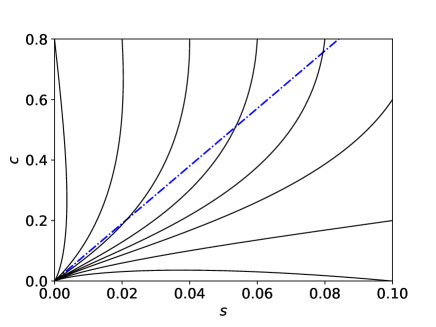
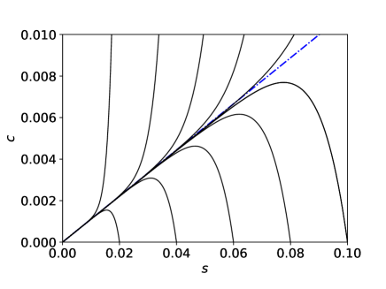
Figure 1: The existence of a sufficiently large spectral gap (thus sufficiently small $\delta$) constitutes the minimal requirement for the validity of a QSS. In both panels, the thin black curves are numerical solutions to the mass action equations (2) for the Michaelis–Menten reaction mechanism. The dashed/dotted blue line is the slow eigenspace. Left: Parameter values: $k_{1}=1.0$, $k_{2}=1.0$, $e_{0}=1.0$ and $k_{-1}=0.01$ and $\delta{\approx}1.0$. Eventually, trajectories approach the origin in a direction that is tangent to the slow eigenspace. However, since the spectral gap is small, tangency manifests very late in the reaction and is so local that it is of little use for any meaningful reduction. Right: Parameter values: $k_{1}=1.0$, $k_{2}=10.0$, $e_{0}=1.0$ and $k_{-1}=0.01$. In this case $\delta{\approx}0.1$, and trajectories quickly approach the origin in the direction of the slow eigenspace.

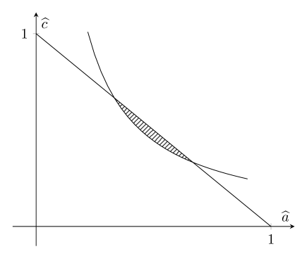
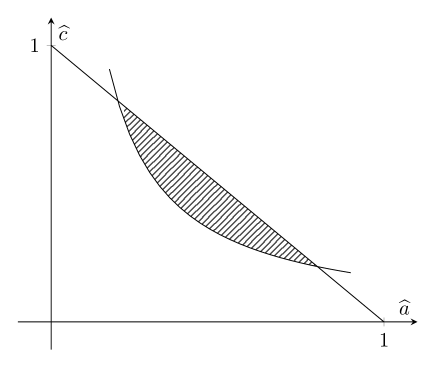
Figure 2: Left: The shaded region coincides with $\delta\geq\frac{1}{2}$. Right The shaded region coincides with $\delta\geq\frac{1}{4}$. Incidentally, the midpoint of the hypotenuse represents $\delta=1$. Geometrically, we see that the majority of parameter combinations satisfy $\delta<1/4$, and very few parameter combinations yield $\delta\geq 1/2.$ Determining the relevant fractions of the triangle area is a matter of basic calculus. One can interpret the shaded region as representing the likelihood that the eigenvalue ratio is bounded below by $1/2$ (Left panel) or $1/4$ (Right panel) if one were to randomly select a parameter ratio $(k_{1}e_{0}:k_{-1}:k_{2})$ . In real-life networks, an eigenvalue ratio $\approx 1$ may be even more infrequent: These ratios occur only when $k_{1}e_{0}\approx k_{2}$ and $k_{-1}\ll k_{2}$, and a meta analysis of parameter estimates from experimental data may reveal that the condition $k_{-1}\ll k_{2}$ is a rare circumstance.

4 The local tangency condition for Michaelis–Menten reaction mechanism

In the previous section, we discussed conditions for QSSA in a broad sense, with no reference to the particular nature of the reduction or the distinguished local manifold. In the present section, we start from some specific QSSA and test the quality of the approximation near the stationary point. Rather than deriving general estimates for local tangency conditions, we focus here on the differential equations for the Michaelis–Menten reaction mechanism (2).

We assume that a candidate for the QSS manifold $Y$ is given in the form $c=g(s)$, with $g(0)=0$. This could be the manifold corresponding to standard QSSA, but also any slow invariant manifold from the list in Patsatzis and Goussis [14], for instance. Note that only $g^{\prime}(0)$ enters computations in the following, thus no explicit form of $g$ is needed. The eigenvalues of the Jacobian at $0$ are

$$\lambda_{1,2}=\frac{1}{2}\left(-(k_{-1}+k_{2}+k_{1}e_{0})\pm\sqrt{(k_{-1}+k_{2}+k_{1}e_{0})^{2}-4k_{1}k_{2}e_{0}}\right),$$

with $|\lambda_{1}|<|\lambda_{2}|$. For the sake of brevity, we disregard the case $k_{-1}=0$ here and in the following.

We say that the QSS manifold $Y$ satisfies the tangency condition at $0$ if the tangent vector $\begin{pmatrix}1\\ g^{\prime}(0)\end{pmatrix}$ is equal to the basis vector $\begin{pmatrix}1\\ \alpha\end{pmatrix}$ of the eigenspace for $\lambda_{1}$. Explicitly,

$$\alpha=\frac{1}{2k_{-1}}\left(-k_{-1}-k_{2}+k_{1}e_{0}+\sqrt{(k_{-1}+k_{2}+k_{1}e_{0})^{2}-4k_{1}k_{2}e_{0}}\right)>0,$$

and

$$\lambda_{1}=-k_{1}e_{0}+k_{-1}\alpha.$$

One will not expect the tangency condition to be satisfied exactly, but it must hold with some degree of accuracy to ensure global accuracy of the QSS reduction. To justify this statement, we will show that violation of the tangency condition, measured by

$$\mu=\left|\dfrac{k_{-1}(g^{\prime}(0)-\alpha)}{\lambda_{1}}\right|,$$ (11)

results in incorrect long-time asymptotics for the substrate concentration.

First, substitution of $c=g(s)$ into the first equation of (2) and linear approximation yields

$$\dot{s}=:h(s)=h^{\prime}(0)s+\text{h.o.t.}=\left(-k_{1}e_{0}+k_{-1}g^{\prime}(0)\right)s+\text{h.o.t.}$$

On the other hand, every solution of system (2) approaches the stationary point tangent to the eigenspace for $\lambda_{1}$, so $c=\alpha s$ up to higher order terms, and we get the correct approximation

$$\dot{s}=\widetilde{h}(s)=\left(-k_{1}e_{0}+k_{-1}\alpha\right)s+\text{h.o.t.}=\lambda_{1}s+\text{h.o.t.},\quad\text{whence }\widetilde{h}^{\prime}(0)=\lambda_{1}.$$

Thus, in the course of approximately linear slow degradation of $s$, the QSSA with the manifold $Y$ given by $c=g(s)$, misrepresents time evolution by a factor

$$\exp\left(|h^{\prime}(0)-\widetilde{h}^{\prime}(0)|t\right)=\exp\left(k_{-1}\left|g^{\prime}(0)-\alpha|\right)t\right).$$

Within a characteristic time $|\lambda_{1}|^{-1}$ for substrate depletion at low concentrations, this QSSA is incorrect by a factor

$$\exp\left(|h^{\prime}(0)-\widetilde{h}^{\prime}(0)|/|\lambda_{1}|\right)=\exp\left(|1-h^{\prime}(0)/\lambda_{1}|\right)=\exp(\mu),$$ (12)

which can be quite large.

We now specialize the discussion and ask under what circumstances is the tangency condition (approximately) valid for the sQSSA, as well as for tQSSA. For both these approximations, we have

$$h^{\prime}(0)=-\dfrac{k_{2}e_{0}}{K_{\rm M}}=-k_{2}\varepsilon_{RS}.$$

Now consider the function

$$\begin{array}[]{rcl}q:&&\,[0,\infty)\to\mathbb{R}\\ x&\mapsto&\frac{1}{2}\left(-(k_{-1}+k_{2}+x)+\sqrt{(k_{-1}+k_{2}+x)^{2}-4k_{2}x}\right)+\dfrac{Kx}{K_{\rm M}}\end{array}$$ (13)

with fixed positive parameters $k_{-1}$, k₂, noting $q(k_{1}e_{0})=\lambda_{1}-h^{\prime}(0)$. As shown in the Appendix 7, $q^{\prime\prime}>0$, hence $q$ is convex, and $q(0)=q^{\prime}(0)=0$. Therefore $q$ is strictly increasing with $x$ and we have $q(k_{1}e_{0})>0$ for positive parameters. This implies

$$|h^{\prime}(0)|>|\lambda_{1}|,\quad\mu=\dfrac{h^{\prime}(0)}{\lambda_{1}}-1>0,$$ (14)

and thus the QSSA always underestimates the timescale for substrate depletion.

We proceed to obtain more palatable estimates for some parameter regions. Using

$$\begin{array}[]{rcl}\widetilde{h}^{\prime}(0)=\lambda_{1}&=&-k_{1}e_{0}+k_{-1}\alpha\\ &=&\cfrac{1}{2}\left(k_{-1}+k_{2}+k_{1}e_{0}\right)\left(-1+\sqrt{1-\dfrac{4Ke_{0}}{(K_{\rm M}+e_{0})^{2}}}\right),\end{array}$$

and the well known inequalities $1-x\leq\sqrt{1-x}\leq 1-x/2$ for $0\leq x\leq 1$, one obtains

$$-\dfrac{2k_{2}e_{0}}{K_{\rm M}+e_{0}}\leq\lambda_{1}\leq-\dfrac{k_{2}e_{0}}{K_{\rm M}+e_{0}},$$

equivalently:

$$-\dfrac{K_{\rm M}+e_{0}}{2k_{2}e_{0}}\geq\dfrac{1}{\lambda_{1}}\geq-\dfrac{K_{\rm M}+e_{0}}{k_{2}e_{0}}.$$ (15)

After some elementary computations we arrive at

$$\dfrac{e_{0}-K_{\rm M}}{2K_{\rm M}}\leq\dfrac{h^{\prime}(0)}{\lambda_{1}}-1\leq\dfrac{e_{0}}{K_{\rm M}},\$$

and thus, given (14), we obtain

$$\ \max\bigg{\{}\dfrac{e_{0}-K_{\rm M}}{2K_{\rm M}},0\bigg{\}}\leq\mu\leq\dfrac{e_{0}}{K_{\rm M}}=\varepsilon_{RS}.\$$

In any case, we see

$$0\leq\mu\leq\varepsilon_{RS},$$ (16)

and therefore the tangency condition improves as $\varepsilon_{RS}\to 0$. But, if $e_{0}>K_{\rm M}$ so that $\varepsilon_{RS}>1$, then

$$\dfrac{1}{2}(\varepsilon_{RS}-1)\leq\mu\leq\varepsilon_{RS},$$ (17)

and we see that the local tangency condition is violated when enzyme is abundant. Consequently, the timescale estimate for slow degradation of substrate is incorrect. Numerical simulations illustrate this fact; see Figure 3. In the Appendix 7, we will provide more detailed estimates, distinguishing various cases for the reaction parameters.

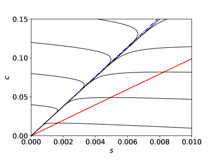
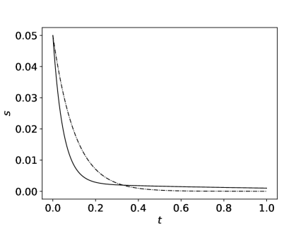
Figure 3: The tangency condition must hold if phase plane trajectories are to approach the QSS manifold towards the origin in the linear regime. Left: The thin black curves are numerical solutions to the mass action equations (2) for the Michaelis–Menten reaction mechanism. The red curve is the QSS manifold corresponding to the $c$-nullcline. The dashed/dotted blue line is the slow eigenspace. Parameter values: $k_{1}=2.0$, $k_{2}=1.0$, $e_{0}=10.0$ and $k_{-1}=1.0$ and $\delta{\approx}0.0413$. Eventually, trajectories approach the origin in a direction that is tangent to the slow eigenspace. However, since the QSS manifold is not tangent to the slow eigenspace, the sQSSA must fail in the long-time limit. Right: The solid black curve is the numerical solution to the mass action equations (2). The dashed/dotted black curve is the numerical solution to the sQSSA. In this example, the QSS manifold is far from tangent to the slow eigenspace. This translates to an erroneous timescale estimate for the degradation of $s$.

At this juncture, it is imperative to recall the precise nature of the tangency condition. As an example, consider the following parameter values: $k_{1}=1.0$, $e_{0}=10.0$, $k_{-1}=10.0$ and $k_{2}=0.01$. It is straightforward to verify that

$$|g^{\prime}(0)-\alpha|{\approx}5\times 10^{-4},$$

and therefore the QSS variety is practically tangent to the slow eigenspace at the origin. However, the sQSSA fails to capture the correct time evolution by a factor

$$\exp(\mu)=\exp\left(k_{-1}\left|g^{\prime}(0)-\alpha\right|/|\lambda_{1}|\right){\approx}2.74.$$

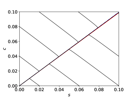
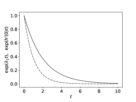
Figure 4: Considering only the phase portrait may be deceptive: “Geometric tangency” of the QSS variety to the slow eigenspace at the origin by itself does not guarantee the long-time validity of the sQSSA. Left: The solid black curves are the numerical solutions to the mass action equations  (2) for the Michaelis–Menten reaction mechanism. The solid red line is the QSS variety, and the broken blue line is the slow eigenspace. Note that these are virtually indistinguishable. Clearly, the phase-plane trajectories approach the origin in the direction of the slow eigenspace, which is practically tangent the QSS variety given by the $c$-nullcline. Right: The sQSS (dashed/dotted black curve) significantly underestimates the characteristic timescale of substrate depletion in the linear regime. The true linear depletion rate is given by the solid black curve. In both panels: $k_{1}=1.0$, $e_{0}=10.0$, $k_{-1}=10.0$, and $k_{2}=0.01$.

This example illustrates that it is not sufficient to consider only the “geometric tangency” of trajectories, as is common practice in the literature on QSSA. The failure of the sQSS in figure (4) is due to the presence of the “amplification term”, $k_{-1}/|\lambda_{1}|$, in (11). A sufficiently large $k_{-1}/|\lambda_{1}|$ can amplify a small difference between $g^{\prime}(0)$ and $\alpha$. The error observed in (4) can be reduced by replacing $c=g(s)$ with an appropriate QSS manifold that improves the geometric tangency. For example, the $\sigma$–isocline of Calder and Siegel [4] approaches the origin exactly tangent to the slow subspace. In dimensional form, the $\sigma$–isocline, $\sigma(s)$, is

$$c=\cfrac{\alpha e_{0}s}{e_{0}+\alpha s}=:\sigma(s).$$ (18)

It is straightforward to verify that $\sigma^{\prime}(s)=\alpha$, and thus $\mu$ is identically zero. Utilizing the $\sigma$–isocline as our QSS variety yields

$$\dot{s}-\cfrac{e_{0}s}{e_{0}+\alpha s}\cdot(k_{1}e_{0}+k_{-1}\alpha),$$ (19)

the linear approximation of which is exactly $\dot{s}=-\lambda_{1}s$. Consequently, the reduction (19) holds nicely near the stationary point; see figure 5, left panel. However, the local validity of (19) does not guarantee its validity in the nonlinear regime; see figure 5, right panel. Hence, local validity does not imply global validity in general.

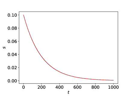
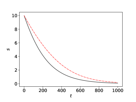
Figure 5: Local validity of a QSS reduction does not imply global validity. Left: In both panels, the solid black curve represents the numerical solution to the mass action equations (2) for the Michaelis–Menten reaction mechanism; the dashed/dotted red curve is the numerical solution to (19). Parameters are $k_{1}=1.0$, $e_{0}=10.0$, $k_{-1}=10.0$, and $k_{2}=0.01$. left: The initial condition used in the simulation is $(s,c)(0)\approx(0.1,0.01)$, and it is clear that (19) is a very good approximation in the linear regime. Right: The initial condition is $(s,c)(0)\approx(10,5)$ and one sees that, outside of the linear regime, the reduced equation (19) (dashed/dotted red curve) dramatically underestimates the rate of substrate depletion. The true linear depletion rate is given by the solid black curve.

5 Short-term versus long-term validity of QSSA

Our results indicate that even for arbitrarily small Heineken et al. [10] parameter $\varepsilon_{HTA}$ or arbitrarily small Segel and Slemrod [21] parameter $\varepsilon_{SSl}$ the QSSA is not necessarily globally accurate. In fact, the initial substrate concentration is of no relevance for long-term QSS. This stands in stark contrast to the widely held belief by practitioners that $e_{0}\ll s_{0}$ is the relevant condition for QSSA.

We will at least partly reconcile these perspectives. In the limit $e_{0}\to 0$, with $s_{0}$ bounded, QSS reduction works indeed by singular perturbation theory, but QSS with increasing $s_{0}$ cannot be traced back to Tikhonov-Fenichel. However, one can actually show that in regions with sufficiently high concentrations of substrate – corresponding to high $s_{0}$ and an early phase of the reaction – the QSS condition holds with good accuracy. For an illustration, see Figure 6.

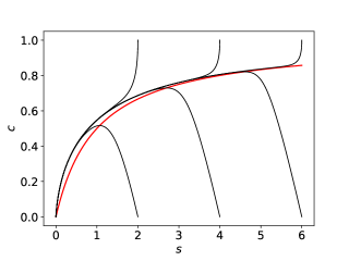
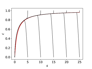
Figure 6: The sQSSA is valid while $s$ is sufficiently large, even in the absence of a spectral gap. The solid black curves are numerical solutions to the mass action equations (2) for the Michaelis–Menten reaction mechanism. The solid red curve is the QSS manifold (i.e., the $c$-nullcline), given by $c=e_{0}s/(K_{\rm M}+s)$. The parameters employed in the simulation are: $k_{1}=e_{0}=k_{2}=1.0$, $s_{0}=25.0$, and $k_{-1}=0$. Thus, $\delta=1$. Observe that even though the eigenvalues of the Jacobian at the origin are equal and therefore the long-time validity of the QSSA fails (Left), the sQSSA still holds for sufficiently large values of $s$, which is illustrated in the Right.

To state our assertion precisely, let us consider a trajectory that starts at $(s_{0},0)$ while it is confined to the region

$$\Lambda:=\{(s,c)\in\mathbb{R}^{2}_{\geq 0}:0\leq c\leq e_{0}\;\;\text{and}\;\;\widehat{s}\leq s\leq s_{0}\},\quad\widehat{s}\geq 0.$$

While $c\leq e_{0}$ holds throughout, $\Lambda$ is not positively invariant whenever $\widehat{s}>0$. From (2) we have

$$\dot{c}=k_{1}(e_{0}-c)s-(k_{-1}+k_{2})c,$$ (20)

and with $e_{0}-c\geq 0$ we obtain the differential inequalities

$$\dot{c} \geq k_{1}(e_{0}-c)\widehat{s}-(k_{-1}+k_{2})c,$$ (21a)

$$\dot{c} \leq k_{1}(e_{0}-c)s_{0}-(k_{-1}+k_{2})c.$$ (21b)

With $c(0)=0$, equation (21) implies

$$c\geq\dfrac{e_{0}\widehat{s}}{K_{\rm M}+\widehat{s}}\left(1-\exp\left(-\widehat{\lambda}t\right)\right),\quad\text{for all }t\text{ such that }(s,c)\in\Lambda,$$ (22)

by standard theorems on differential inequalities, where $\widehat{\lambda}:=k_{1}\widehat{s}+k_{-1}+k_{2}$. Likewise, it also holds that

$$c\leq\dfrac{e_{0}s_{0}}{K_{\rm M}+s_{0}}\left(1-\exp\left(-\lambda_{0}t\right)\right),\quad\text{ for all }t\geq 0,$$ (23)

where $\lambda_{0}:=k_{-1}+k_{2}+k_{1}s_{0}$. Finally, using (2) with “frozen” $s\in[\widehat{s},s_{0}]$ and invoking differential inequalities again, we arrive at

$$\widehat{L}:=\dfrac{e_{0}\widehat{s}}{K_{\rm M}+\widehat{s}}\leq\dfrac{e_{0}s}{K_{\rm M}+s}\leq\dfrac{e_{0}s_{0}}{K_{\rm M}+s_{0}}=:L_{0}$$ (24)

by taking the limit $t\to\infty$. Moreover, for large $\widehat{\lambda}$ we see that the terms on the right hand sides of (22) and (23) quickly approach their respective limits, $\widehat{L}$ and $L_{0}$. From Proposition 2 by Noethen and Walcher [11] (see also Calder and Siegel [4]), it is known that the trajectory starting at $(s_{0},0)$ crosses the QSS manifold $Y$. From Proposition 12 by Noethen and Walcher [11], after a characteristic time that is ${O}(1/|\widehat{\lambda}|)$, it holds that $\widehat{L}\leq c\leq L_{0}.$ Furthermore, the distance between $\widehat{L}$ and $L_{0}$ is given by

$$L_{0}-\widehat{L}=\cfrac{K_{\rm M}(s_{0}-\widehat{s})e_{0}}{(K_{\rm M}+\hat{s})(K_{\rm M}+s_{0})}\ ,$$

which is practically negligible whenever $K_{\rm M}\ll\widehat{s}$ and $e_{0}$ bounded. For instance, with $\widehat{s}=s_{0}/2$ one has

$$L_{0}-\widehat{L}=L_{0}\cdot\cfrac{K_{\rm M}}{2(K_{\rm M}+\widehat{s})}.$$

Consequently, the phase plane trajectory will remain very close to the QSS manifold everywhere in $\Lambda$ where $K_{\rm M}\ll\widehat{s}$. In this sense, the QSS for complex is valid. For a numerical validation, please see Figure 7.

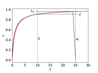
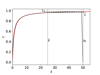
Figure 7: The QSS is valid in domains where $s\geq\widehat{s}$, with $K_{\rm M}/\widehat{s}$ sufficiently small. In both numerical simulations, the solid black curve is the numerical solution to the mass action equations (2) for the Michaelis–Menten reaction mechanism. The solid red curve is the QSS manifold (i.e., the $c$-nullcline), given by $c=e_{0}s/(K_{\rm M}+s)$. The dashed/dotted lines correspond to the limits $L_{0}$ and $\widehat{L}$. The locations of $s_{0}$ and $\widehat{s}$ are demarcated by dotted vertical lines. Left: The parameters employed in the simulation are: $k_{1}=e_{0}=k_{2}=1.0$, $s_{0}=25.0$, $k_{-1}=0$ $s_{0}=25$ and $\widehat{s}=10$. Observe that, after a brief transient, the trajectory closely follows the QSS manifold for $s\in[\widehat{s},s_{0}]$, but departs from the QSS manifold as it approaches the origin. Right: The parameters employed in the simulation are: $k_{1}=e_{0}=k_{2}=1.0$, $s_{0}=25.0$, $k_{-1}=0$ $s_{0}=50$ and $\widehat{s}=25$. Observe that the distance between the upper and lower limits diminishes as $\widehat{s}/K_{\rm M}$ increases.

It is clear from Figure 7 that large initial substrate concentration will ensure the temporary validity of the QSSA but, without a sufficient spectral gap, the sQSSA will lose accuracy once $s\lesssim K_{\rm M}$. One can also invoke the following argument to understand that increasing $s_{0}$ cannot improve the quality of the QSS reduction over the full course of the reduction: Moving a point along a trajectory just amounts to translation of time, which leaves the long-term behavior unaffected.

Moreover, this loss may be consequential in the context of progress curve experiments utilized to estimate $K_{\rm M}$ and the maximal turnover rate $V=k_{2}e_{0}$ by fitting time-course data to the sQSSA. According to Stroberg and Schnell [22], measurements should be taken with $s$ near $K_{\rm M}$, as the inverse problem is ill-posed in regions where the QSS variety is extremely flat, i.e., where $K_{\rm M}\ll s$. The questionable quality of parameter fitting also turns up in the initial rate experiments with varying, but high initial substrate concentrations $s_{0}$, since all the data points for regression to determine the Lineweaver-Burk line lie close to the ordinate, and thus proper extrapolation becomes doubtful. The same challenge will apply to initial rate experiments carrying out parameter estimation to a non-linear fitting of the Michaelis–Menten equation (3). Consequently, an overabundant concentration of substrate may not be strategically beneficial for parameter estimation applications, and thus we see that the local validity of the QSSA has experimental (in addition to merely mathematical) relevance. The inverse modeling problem of parameter estimation needs to be investigated systematically based on the findings of this work.

6 Discussion

In Section 3 the validity of local QSSA for the Michaelis–Menten reaction mechanism has been reconsidered, and has been shown to be fully compatible with the fundamental requirement of eigenvalue disparity. The eigenvalue disparity conditions are the same as those given by Patsatzis and Goussis [14], specialized to the stationary point, and they are also present in earlier work by Palsson and Lightfoot [13]. But (implicitly) in these works the eigenvalue conditions have only been considered with sufficiency in mind. From a mathematical perspective, in order to prove that the conditions are also necessary, one has to establish that QSSA actually fails when they are violated. This is the new aspect in the present work, where we have determined, quantitatively, a region in parameter space where any type of QSS fails to hold (anti-QSS) due to the absence of a sufficiently large spectral gap. The fact that a random choice of reaction parameters will likely lie outside this region, may explain the widely held belief that some type of QSSA (even more specifically, tQSSA) is roughly valid for all parameters. On the other hand, the analysis by Patsatzis and Goussis [14] shows conclusively that some type of QSSA does hold in large regions of parameter space.

Furthermore, in Section 4 we have shown that, for any given QSSA, the approximate tangency of the QSS variety to the slow eigenspace of the stationary point (characterized by $\mu\ll 1$, with $\mu$ given in (11)) is necessary to ensure good approximation by the QSS reduction. For the sQSSA and tQSSA, we have shown that the Reich and Selkov [16] condition, $e_{0}\ll K_{\rm M}$, ensures the long-time validity of the sQSSA, as this condition ensures the existence of a spectral gap as well as the tangency condition, $\mu\ll 1$. Note that this condition does not involve initial substrate.

We address the difference between the commonly used parameters due to Heineken et al. [10], respectively to Segel and Slemrod [21], and the ones derived in the present paper. The discrepancy is due to Segel’s choice of a nonlinear timescale estimate, and we showed that it may provide incorrect predictions for the existence and the nature of a reduction over the whole time course. In a way, this is not unexpected. Initial conditions can be moved along trajectories, and this does not influence the long-term behavior.

Our analysis has resulted in a considerably clearer understanding of the QSSA, and also our discussion points the way to an improvement in a general technique of applied mathematics. There are important lessons to be drawn from the anti-QSSA. A number of papers in the literature assume that certain QSS reductions will always be roughly valid across the full parameter space. Our results show that this is not the case. More importantly, the conditions for the anti-QSSA presents an important opportunity to assert the region of the parameter domain where no QSSA can be applied to model systems or use QSS reduction to estimate parameters. This is an important subject of active research in rigor and reproducibility [9, 22].

The moral of this paper seems to be that estimating the validity of QSS reductions is not as mechanical as it appears. For planar systems, any qualifier (i.e., dimensionless parameter) claiming to certify the legitimacy of a QSS reduction must, at minimum, satisfy the requirements discussed in this work. Based on our survey of the QSS literature, it appears that intuitive scaling arguments sometimes produce qualifiers that fail to meet these obligations. The fundamental requirements highlighted in this work should be considered in future applications if progress in deterministic QSS theory (and possibly stochastic QSS theory) is to advance. Moreover, the extensive utilization of QSS reduction in mathematical biology and applied mathematics suggests that additional progress is indispensable.

7 Appendix

Here we provide some details on the function $q$ introduced in Section 4, and proceed to obtain sharper estimates on the parameter $\mu$.

Differentiating the expression in (13), one finds

$$q^{\prime}(x)=-\frac{1}{2}+\frac{k_{2}}{k_{-1}+k_{2}}+\frac{1}{2}\cdot\dfrac{x+k_{-1}-k_{2}}{\left((x+k_{-1}+k_{2})^{2}-4k_{2}x\right)^{1/2}}$$

and furthermore

$$q^{\prime\prime}(x)=\dfrac{2k_{-1}k_{2}}{\left((x+k_{-1}+k_{2})^{2}-4k_{2}x\right)^{3/2}}>0\text{ for }x>0,$$ (25)

which implies all the assertions in Section 4.

More detailed estimates start from observing

$$q(x)=q^{\prime\prime}(\xi)\cdot x^{2}\text{ for some }\xi,\quad 0\leq\xi\leq x,$$ (26)

by Taylor’s theorem, and from upper and lower estimates for the maximum and minimum of $q^{\prime\prime}(\xi)$ on the interval $[0,x]$. As evident from (25), this maximum and minimum correspond to the minimum and maximum (in this order) of the quadratic function

$$\eta(\xi):=(\xi+k_{-1}+k_{2})^{2}-4k_{2}\xi=(\xi+k_{-1}-k_{2})^{2}+4k_{-1}k_{2}\text{ on }[0,x].$$ (27)

One has to distinguish cases now:

• In case $k_{-1}\geq k_{2}$, the minimum appears at $\xi=0$, with value $(k_{-1}+k_{2})^{2}$, and the maximum appears at $\xi=x$.

• In case $k_{-1}<k_{2}$ and $x\leq 2(k_{2}-k_{-1})$, the minimum appears at $\xi=k_{2}-k_{-1}$, with value $4k_{-1}k_{2}$, and the maximum appears at $\xi=0$.

• In case $k_{-1}<k_{2}$ and $x>2(k_{2}-k_{-1})$, the minimum appears at $\xi=k_{2}-k_{-1}$, with value $4k_{-1}k_{2}$, and the maximum appears at $\xi=x$.

Thus, for instance, in case $k_{-1}\geq k_{2}$ the maximum of $q^{\prime\prime}$ appears at $\xi=0$, with value $2k_{-1}k_{2}/(k_{-1}+k_{2})^{3}$, and one gets

$$\lambda_{1}-h^{\prime}(0)\leq\dfrac{2k_{-1}k_{2}\,(k_{1}e_{0})^{2}}{(k_{-1}+k_{2})^{3}}.$$

Combining this with the estimate from (15) one arrives at

$$\mu=\dfrac{h^{\prime}(0)}{\lambda_{1}}-1\leq\dfrac{2k_{-1}\cdot(k_{-1}+k_{2}+k_{1}e_{0})\cdot k_{1}e_{0}}{(k_{-1}+k_{2})^{3}}\leq\dfrac{2k_{-1}\cdot k_{1}e_{0}}{(k_{-1}+k_{2})^{2}}.$$ (28)

One can work through all the cases in a similar manner, with the following results:

• In case $k_{-1}\geq k_{2}$, one has the upper estimates (28) for $\mu$, and the lower estimates

  $$\mu\geq\dfrac{k_{-1}\cdot(k_{-1}+k_{2}+k_{1}e_{0})\cdot k_{1}e_{0}}{\left((k_{-1}+k_{2}+k_{1}e_{0})^{2}-4k_{2}k_{1}e_{0}\right)^{3/2}}\geq\dfrac{k_{-1}\cdot k_{1}e_{0}}{\left(k_{-1}+k_{2}+k_{1}e_{0}\right)^{2}}.$$ (29)

• In case $k_{-1}<k_{2}$ one gets the upper estimates

  $$\mu\leq\dfrac{(k_{-1}+k_{2}+k_{1}e_{0})\cdot k_{1}e_{0}}{4k_{-1}^{1/2}k_{2}^{3/2}}\leq\dfrac{(k_{-1}+k_{2}+k_{1}e_{0})\cdot k_{1}e_{0}}{4k_{-1}^{2}}.$$ (30)

  Furthermore:

  • In case $k_{1}e_{0}\leq 2(k_{2}-k_{-1})$ one obtains the lower estimates

    $$\mu\geq\dfrac{k_{-1}\cdot(k_{-1}+k_{2}+k_{1}e_{0})\cdot k_{1}e_{0}}{(k_{-1}+k_{2})^{3}}\geq\dfrac{k_{-1}\cdot k_{1}e_{0}}{(k_{-1}+k_{2})^{2}}.$$ (31)

  • In case $k_{1}e_{0}>2(k_{2}-k_{-1})$ one obtains the lower estimate

    $$\mu\geq\dfrac{k_{-1}\cdot(k_{-1}+k_{2}+k_{1}e_{0})\cdot k_{1}e_{0}}{\left((k_{-1}+k_{2}+k_{1}e_{0})^{2}-4k_{2}k_{1}e_{0}\right)^{3/2}}\geq\dfrac{k_{-1}\cdot k_{1}e_{0}}{\left(k_{-1}+k_{2}+k_{1}e_{0}\right)^{2}}.$$ (32)

These estimates are more detailed than the ones presented in the main part of the paper, and in particular one obtains positive lower bounds for $\mu$ in every case. But the necessary distinction of cases may offset the advantage in applications. Note that we do not aggregate the rate constants in terms of $K$ and $K_{\rm M}$ in this Appendix.

References

- [1] J.A.M. Borghans, R.J. de Boer, L.A. Segel: Extending the quasi-steady state approximation by changing variables. Bull. Math. Biol. 58, 43–63 (1996).
- [2] G.E. Briggs, J.B.S Haldane: A note on the kinetics of enzyme action, Biochem. J. 19, 338-339 (1925).
- [3] A.D. Bruno: Local methods in nonlinear differential equations. Springer-Verlag, Berlin (1989).
- [4] M.S. Calder, D. Siegel: Properties of the Michaelis-–Menten mechanism in phase space. J. Math. Anal. Appl. 339, 1044–-1064 (2008).
- [5] C. Chicone: Ordinary differential equations with applications. Second edition. Springer, New York (2006).
- [6] J. Eilertsen, M.R. Roussel, S. Schnell, S. Walcher: On the quasi-steady-state approximation in an open Michaelis–Menten reaction mechanism. AIMS Math. 6, no. 7, 6781–6814 (2021).
- [7] N. Fenichel: Geometric singular perturbation theory for ordinary differential equations. J Differ. Equ. 31(1), 53–98 (1979).
- [8] A. Goeke, S. Walcher, E. Zerz: Classical quasi-steady state reduction – A mathematical characterization. Physica D 345, 11–26 (2017).
- [9] P. Halling, P. Fitzpatrick, F. M. Raushel, J. Rohwer, S. Schnell, U. Wittig, R. Wohlgemuth, C. Kettner: An empirical analysis of enzyme function reporting for experimental reproducibility: Missingincomplete information in published papers, Biophys. Chem. 242, 22–27 (2018).
- [10] F.G. Heineken, H.M. Tsuchiya, R. Aris: On the mathematical status of the pseudo-steady hypothesis of biochemical kinetics. Math. Biosci. 1, 95–113 (1967).
- [11] L. Noethen, S. Walcher: Quasi-steady state in the Michaelis–Menten system. Nonlinear Anal. Real World Appl. 8, 1512–1535 (2007).
- [12] B.O. Palsson: Systems Biology: Simulation of Dynamic Network States. Cambridge University Press (2011).
- [13] B.O. Palsson, E.N. Lightfoot: Mathematical modellling of dynamics and control in metabolic networks. I. On Michaelis–Menten kinetics. J. Theor. Biol. 111, 273–302 (1984).
- [14] D.G. Patsatzis, D.A. Goussis: A new Michaelis–Menten equation valid everywhere multi-scale dynamics prevails. Math. Biosci. 315, 108220, 13 pp. (2019).
- [15] L. Perko: Differential equations and dynamical systems, 3rd Edition. Springer, New York (2001).
- [16] J.G. Reich, E.E. Selkov: Mathematical analysis of metabolic networks. FEBS Letters 40, Suppl. 1, S119–S127 (1974).
- [17] M.R. Roussel, S.J. Fraser: Geometry of the steady‐state approximation: Perturbation and accelerated convergence methods. J. Chem. Phys. 93, 1072–1081 (1990).
- [18] M. Schauer, R. Heinrich: Analysis of the quasi-steady-state approximation for an enzymatic one-substrate reaction. J. Theor. Biol. 79, 425–442 (1979).
- [19] S. Schnell, P.K. Maini: Enzyme kinetics far from the standard quasi-steady-state and equilibrium approximations. Math. Comput. Modelling 35, 137–144 (2002).
- [20] L.A. Segel: On the validity of the steady state assumption of enzyme kinetics. Bull. Math. Biol. 50, 579–593 (1988).
- [21] L.A. Segel, M. Slemrod: The quasi-steady-state assumption: A case study in perturbation. SIAM Rev. 31, 446–477 (1989).
- [22] W. Stroberg, S. Schnell: On the estimation errors of and from time-course experiments using the Michaelis-–Menten equation, Biophys. Chem. 219, 17–27 (2016).
- [23] A.N. Tikhonov: Systems of differential equations containing a small parameter multiplying the derivative (in Russian). Math. Sb. 31, 575–586 (1952).
- [24] A.R. Tzafriri: Michaelis–Menten kinetics at high enzyme concentrations. Bull. Math. Biol. 65, 1111–1129 (2003).
- [25] F. Verhulst: Methods and Applications of Singular Perturbations. Boundary Layers and Multiple Timescale Dynamics, Springer, New York (2005).
- [26] S. Walcher: On the Poincaré problem. J Differ. Equ. 166, 51–78 (2000).