SASG: Sparse Communication with
Adaptive Aggregated Stochastic Gradients
for Distributed Learning

Abstract

Stochastic optimization algorithms implemented on distributed computing architectures are increasingly used to tackle large-scale machine learning applications. A key bottleneck in such distributed systems is the communication overhead for exchanging information such as stochastic gradients between different workers. Sparse communication with memory and the adaptive aggregation methodology are two successful frameworks among the various techniques proposed to address this issue. In this paper, we exploit the advantages of Sparse communication and Adaptive aggregated Stochastic Gradients to design a communication-efficient distributed algorithm named SASG. Specifically, we determine the workers who need to communicate with the parameter server based on the adaptive aggregation rule and then sparsify the transmitted information. Therefore, our algorithm reduces both the overhead of communication rounds and the number of communication bits in the distributed system. We define an auxiliary sequence and provide convergence results of the algorithm with the help of Lyapunov function analysis. Experiments on training deep neural networks show that our algorithm can significantly reduce the communication overhead compared to the previous methods, with little impact on training and testing accuracy.

1 Introduction

Over the past few decades, the scale and complexity of Machine-Learning (ML) models and datasets have increased significantly [1, 2], leading to more computation intensity and giving the impetus to the development of distributed training [3, 4, 5]. A large number of distributed machine learning tasks can be described as

$$\min_{\omega\in\mathbb{R}^{d}}~{}F(\omega):=\frac{1}{M}\sum_{m\in\mathcal{M}}\mathbb{E}_{\xi_{m}\sim\mathcal{D}_{m}}\left[f_{m}(\omega;\xi_{m})\right],$$ (1)

where $\omega$ is the parameter vector to be learned, $d$ is the dimension of parameters, and $\mathcal{M}:=\{1,\dots,M\}$ denotes the set of distributed workers. $\{f_{m}\}_{m=1}^{M}$ are smooth (unnecessary to be convex) loss functions kept at worker $m$, and $\{\xi_{m}\}_{m=1}^{M}$ are independent random data samples associated with probability distribution $\{\mathcal{D}_{m}\}_{m=1}^{M}$. For simplicity, we define $F_{m}(\omega):=\mathbb{E}_{\xi_{m}\sim\mathcal{D}_{m}}\left[f_{m}(\omega;\xi_{m})\right]$; let $\omega^{*}$ be the optimal solution and $F^{*}:=F(\omega^{*})$. Problem (1) arises in a large number of distributed machine learning tasks, ranging from linear models to deep neural networks [5, 6].

Stochastic Gradient Descent (SGD) is the workhorse for problem (1), performing as

$$\omega^{t+1}=\omega^{t}-\gamma\cdot\frac{1}{M}\sum_{m\in\mathcal{M}}\nabla f_{m}(\omega^{t};\xi_{m}^{t}),$$ (2)

where $\gamma$ is the learning rate, and $\xi_{m}^{t}$ is the mini-batch data selected by worker $m$ at the $t$-th iteration. The commonly-used Parameter-Server (PS) architecture is studied in [4, 7], where $M$ workers compute the gradients in parallel, and a centralized server updates the variable $\omega$. The implementation details of distributed SGD method are as follows: at iteration $t$, the server broadcasts $\omega^{t}$ to all workers; every worker $m\in\mathcal{M}$ computes the local gradient $\nabla f_{m}(\omega^{t};\xi_{m}^{t})$ with a randomly selected mini-batch of samples $\xi_{m}^{t}\sim\mathbb{D}_{m}$ and uploads it to the server; the server can simply use the aggregated gradient, i.e., $\sum_{m\in\mathcal{M}}\nabla f_{m}(\omega^{t};\xi_{m}^{t})$, to update the parameters via (2). The convergence of this distributed implementation of SGD has been proved under several mild assumptions [8].

Intuitively, multi-processor collaborative training for one task can accelerate the training process and reduce training time. However, the communication cost between processors usually hampers the scalability of distributed systems [9, 10]. More specifically, at each iteration of PS training (2), the server needs to communicate with all workers to obtain fresh gradients $\{\nabla f_{m}(\omega^{t};\xi_{m}^{t})\}_{m=1}^{M}$, which may lead to unaffordable communication overhead in systems with limited communication resources such as energy and bandwidth. Even worse, when the computation-to-communication ratio is low, e.g., using high-speed computing devices with low-speed interconnect to train a ML model, multiple processors may suffer lower performance than a single processor [11]. Therefore, the communication overhead between workers and the server has become a major bottleneck.

Various popular techniques have been proposed to alleviate this problem, including sparse communication [12, 13, 14, 15] and adaptive aggregation methods [16, 17, 18]. The former is dedicated to compressing each gradient information $\nabla f_{m}(\omega^{t};\xi_{m}^{t})$, while the latter focuses on reducing the number of communications $M$. Since these two techniques are orthogonal, a natural question is then can we combine the two approaches to yield a better mechanism for problem (1)?

This paper gives an affirmative answer to this question. We aim to develop a communication-efficient algorithm that simultaneously reduces the number of communication rounds and bits without sacrificing convergence.

Since communication rounds between the server and workers are unequally important in the distributed learning system, we can adjust the frequency of communication between a worker and the server according to the importance of the transmitted information. More specifically, to reduce the number of communication rounds, we have formulated an adaptive selection rule to divide the set of workers $\mathcal{M}$ into two disjoint sets, $\mathcal{M}^{t}$ and $\mathcal{M}_{c}^{t}$, at the $t$-th iteration. We will use only the new gradient information from the selected workers in $\mathcal{M}^{t}$ while reusing the outdated gradients from the rest of the workers in $\mathcal{M}_{c}^{t}$, scaling down the per-iteration communication rounds from $M$ to $|\mathcal{M}^{t}|$.

To reduce communication bits, we will further compress the communicated information. Our algorithm adopts a more aggressive sparsification method as the quantization methods can only achieve a maximum compression rate of 32$\mathsf{x}$ over the commonly used SGD with single-precision floating-point arithmetic. Specifically, we will select the top-$k$ gradient coordinates (ordered by absolute value) at each iteration and zero the rest of the gradient terms, making the zero-valued elements free from communication and thus significantly reducing the number of communication bits.

In terms of theoretical analysis, we first give a new insight to demonstrate the effectiveness of our adaptive selection rule. Furthermore, the error feedback technique, i.e., incorporating the error made by the sparsification operator into the next step, was employed to deal with the biased nature of the top-$k$ sparsification operator. Lyapunov analysis of an auxiliary sequence shows that SASG is convergent and achieves a sublinear convergence rate despite skipping many communication rounds and performing communication compression.

Contributions. This paper focuses on reducing the worker-to-server uplink communication overhead in the PS architecture, which we also refer to as upload. As opposed to the server-to-worker downlink communication (i.e., broadcast the same parameter $\omega$) that can be performed simultaneously or implemented in a tree-structured manner as in many MPI implementations, the server must receive gradients of workers sequentially to avoid interference from other workers, which leads to extra latency. Therefore, uploads are the primary communication overhead in PS and the subject of many related works [19, 20, 18, 21]. Throughout this paper, one communication round means one upload from a worker. The contributions can be summarized as follows:

• We propose a communication-efficient algorithm for distributed learning which can reduce both communication rounds and bits.

• We define a crucial auxiliary sequence and develop a new Lyapunov function to establish the convergence analysis of SASG. The convergence rate matches that of the original SGD.

• We conduct extensive experiments to demonstrate the superiority of the proposed SASG algorithm.

The rest of the paper is organized as follows. Section 2 reviews two categories of related work on improving the communication efficiency of distributed systems. Then, we present the development details and workflow of the SASG algorithm in Section 3. Theoretical analysis and experimental validation of SASG are given in Sections 4 and 5, respectively. Section 6 contains the proof details, and Section 7 concludes this study.

Notation. Throughout the paper, $\mathbb{E}[\cdot]$ denotes the expectation taken for the randomly selected data sample. For a vector $\mathbf{x}\in\mathbb{R}^{d}$, $\|\mathbf{x}\|$ and $|\mathbf{x}|$ represent its $\ell_{2}$-norm and the absolute value of $\mathbf{x}$, respectively. $[d]$ is the set $\{1,2,\cdots,d\}$, and $|\mathcal{S}|$ denotes the number of elements in the set $\mathcal{S}$.

2 Related Work

A tremendous amount of communication-efficient distributed learning approaches have been proposed to take full advantage of the computational power of distributed clusters [22, 16, 23, 24, 17, 25, 20, 18, 26, 27, 19, 28, 29, 30, 21]. More information can be found in a comprehensive survey [31]. We briefly review two kinds of related work in this paper: 1). from the perspective of what to communicate, the number of transmitted bits per communication round can be reduced via quantization or sparsification, and 2). from the perspective of when to communicate, some communication rules are used to save the number of communication rounds.

2.1 Communication Bit Reduction

This category of research is mainly around the idea of quantization and sparsification.

The quantization approach compresses the information by transmitting lower bits instead of the data originally represented by 32 bits on each dimension of the transmitted gradient. Quantized Stochastic Gradient Descent (QSGD) [30] utilizes an adjustable quantization level, allowing additional flexibility to control the trade-off between the per-iteration communication cost and the convergence rate. TernGrad [21] uses the ternary gradients to reduce the communication data size. 1-bit quantization method was developed in [32, 33], which reduces each component of the gradient to just its sign (one bit). Adaptive quantization methods are also investigated in [34] to reduce the communication cost.

The sparsification method reduces the number of elements transmitted at each iteration. Such methods can be divided into two main categories: random and deterministic sparsification. Random sparsification [35, 29] is to select some entries to communicate randomly. This ideology is named random-$k$, where $k$ denotes the number of selected elements. This random choice method is usually an unbiased estimate of the original gradient, making it quite friendly to theoretical analysis. Unlike random sparsification, deterministic sparsification [12, 13, 14, 15] preserves only a few coordinates of the stochastic gradient with the largest magnitudes. This ideology is also known as top-$k$. In contrast to the unbiased scheme, it is clear that this approach needs to work with the error feedback or accumulation procedure [23, 36, 13, 37] for convergence.

2.2 Communication Round Reduction

Reducing the number of communication rounds to improve communication efficiency is another research focus. Shamir et al. [38] leveraged higher-order information (newton-type method) to replace traditional gradient information, thereby reducing the number of communication rounds. Hendrikx et al. [39] proposed a distributed preconditioned accelerated gradient method to reduce the number of communication rounds. Novel aggregation techniques, such as periodic aggregation [19, 40, 26] and adaptive aggregation [18, 20, 16], are also investigated and used to skip certain communications. Among them, local SGD [40, 26] allows every worker to perform local model updates independently, and the resultant models are averaged periodically. Lazily Aggregated Gradient (LAG) [18] updates the model at the server-side, and workers only adaptively upload information that is determined to be informative enough. Unfortunately, while the original LAG has good performance in the deterministic settings (i.e., with full gradient), its performance in the stochastic setting degrades significantly [17]. Recent efforts have been made toward adaptive uploading in stochastic settings [17, 25]. Communication-Censored distributed Stochastic Gradient Descent (CSGD) [25] algorithm increases the batch size to alleviate the effect of stochastic gradient noise. Lazily Aggregated Stochastic Gradient (LASG) [17] designed a set of new adaptive communication rules tailored for stochastic gradients, achieving impressive empirical performance.

We borrowed some ideas from LASG here. The main difference is that LASG reduces the overhead of communication rounds only, and we extend this work so that our SASG method can reduce the overhead of both communication rounds and bits in the stochastic setting. In addition, we also reduce the memory overhead required for the adaptive aggregation technique as SASG only need to keep the sparsified data on the server side.

Figure 1: SASG overview. At the $t$-th iteration, the parameter server broadcasts ${\omega}^{t}$ to all workers, and workers in $\mathcal{M}^{t}$ (marked in green) will upload the sparsified gradient information $\mathcal{T}_{k}(g_{m}^{t})$ and reset $\tau_{m}^{t+1}=1$; while workers in $\mathcal{M}_{c}^{t}$ (marked in pink) will increase the staleness by $\tau_{m}^{t+1}=\tau_{m}^{t}+1$ and upload nothing; then the server updates parameter $\omega$ via (8).

3 Algorithm development

We introduce SASG, a communication-efficient distributed algorithm that reduces both the number of communication rounds and bits. We first describe the motivation and challenges for developing this method and then present the scheme of the proposed algorithm.

3.1 Motivation and Challenges

In the distributed learning system, an important finding is that not all communication rounds between the server and workers contribute equally to the state of the global model [18, 17, 16, 27]. Then one can design an aggregation rule to skip the inefficient communication rounds. LAG develops an adaptive selection rule, which can detect workers with slowly-varying gradients and triggers the reuse of outdated gradients, thus improving communication efficiency.

However, this technique only reduces the number of communication rounds and requires additional memory overhead on the server-side, which is far from enough in resource-limited scenarios. Indeed, we can do more beyond LAG, e.g., reduce the transmitted bits of uploaded information rather than just the rounds, and reduce the server-side storage overhead.

There are always two lines of transmission bit reduction: quantization and sparsification. We employ the latter as quantization methods can only reach a maximum compression rate of 32$\mathsf{x}$ (1-bit quantization method) in the commonly used single-precision floating-point algorithms. When the dimension $d$ of the model is large, i.e., $d\gg 32$, the sparsification method will far outperform the quantization approach (the maximum compression rate of $d\times$ may be reached).

Although random sparsification methods guarantee the unbiasedness of the compression operator and facilitate theoretical analysis, the top-$k$ sparsification method tends to achieve better practical results [35, 13]. We will apply the top-$k$ sparsification operator, namely $\mathcal{T}_{k}(\cdot)$. This operator retains only the largest $k$ components (in absolute value) of the gradient vector, and the specific definition is as follows.

Definition 1

For a parameter $1\leq k<d$, the sparsification operator $\mathcal{T}_{k}(\cdot):\mathbb{R}^{d}\rightarrow\mathbb{R}^{d}$, is defined for $\mathbf{x}\in\mathbb{R}^{d}$ as

$$\left(\mathcal{T}_{k}(\mathbf{x})\right)_{\pi(i)}:=\left\{\begin{array}[]{ll}(\mathbf{x})_{\pi(i)},&\text{ if }i\leq k,\\ 0,&\text{ otherwise },\end{array}\right.$$ (3)

where $\pi$ is a permutation of set $[d]$ such that $(|\mathbf{x}|)_{\pi(i)}\geq(|\mathbf{x}|)_{\pi(i+1)}$ for $i=1,\ldots,d$.

Nevertheless, this combination encounters two main challenges. 1). How to design an effective communication criterion in the sparsification setting? That is, in this composite situation, we need to determine which communications are non-essential exactly. 2). How can we guarantee model convergence when updating the parameters with only sparsified information from a subset of workers? In particular, the only partial information we have is still biased. Our approach will address these challenges.

3.2 SASG Method

We first need to determine an effective selection criterion to address challenge 1. Intuitively, if the difference between two consecutive gradients from a worker is small, it is safe to skip the redundant uploads and reuse the previous one in the server. The difference is defined as

$$\Delta_{m}^{t}:=\nabla f_{m}({\omega}^{t};\xi_{m}^{t})-\nabla f_{m}({\omega}^{t-\tau_{m}^{t}};\xi_{m}^{t-\tau_{m}^{t}}),$$ (4)

where $\tau_{m}^{t}$ is the delay count. In addition, we need to pick a threshold that varies with iteration $t$ to adaptively measure the magnitude of the difference $\Delta_{m}^{t}$. Following the idea of LAG, we have

$$\Delta_{m}^{t}\leq\frac{1}{M^{2}}\sum_{d=1}^{D}\alpha_{d}\left\|\omega^{t+1-d}-\omega^{t-d}\right\|^{2},$$ (5)

where $\{\alpha_{d}\geq 0\}_{d=1}^{D}$ are constant weights. This rule is a direct extension of LAG to the stochastic settings. Unfortunately, (5) is ineffective due to the non-diminishing variance of the stochastic gradients (i.e., $\Delta_{m}^{t}$ has almost never been small). Our SASG method takes advantage of the adaptive selection rule of LASG [17], formulated as

$$\begin{split}&\left\|\nabla f_{m}({\omega}^{t};\xi_{m}^{t})-\nabla f_{m}({\omega}^{t-\tau_{m}^{t}};\xi_{m}^{t})\right\|^{2}\\ &\qquad\leq\frac{1}{M^{2}}\sum_{d=1}^{D}\alpha_{d}\left\|\omega^{t+1-d}-\omega^{t-d}\right\|^{2}.\end{split}$$ (6)

This condition is evaluated on the same data $\xi_{m}^{t}$ at two different iterations $t$ and $t-\tau_{m}^{t}$. We will give a new insight to show that the criterion is applicable. According to the Lipschitz continuous property of $\nabla f_{m}$, we have

$$\begin{split}&\left\|\nabla f_{m}({\omega}^{t};\xi_{m}^{t})-\nabla f_{m}({\omega}^{t-\tau_{m}^{t}};\xi_{m}^{t})\right\|^{2}\\ &\qquad\leq L_{m}\left\|\omega^{t}-\omega^{t-\tau_{m}^{t}}\right\|^{2},\end{split}$$ (7)

where $L_{m}$ is the Lipschitz constant. As the iterative sequence $\{\omega^{t}\}_{t=0,1,\ldots}$ converges, the right-hand side of (7) diminishes, and thus the left-hand side of (6) diminishes, which eliminates the inherent variance caused by stochastic data $\xi_{m}^{t}$ and $\xi_{m}^{t-\tau_{m}^{t}}$.

At each training iteration $t$, selection rule (6) will divide the set of worker $\mathcal{M}$ into two disjoint sets, $\mathcal{M}^{t}$ and $\mathcal{M}_{c}^{t}$. The parameter server only needs to receive the new gradient information from $\mathcal{M}^{t}$ and reuse the outdated gradients (stored on the server-side) from $\mathcal{M}_{c}^{t}$, which scale down the per-iteration communication rounds from $M$ to $|\mathcal{M}^{t}|$. After the adaptive selection procedure, selected workers will send the sparse information derived by the top-$k$ operator to the parameter server, which reduces the communication bits and the memory overhead on the server-side. However, the biased nature of the top-$k$ operator breaks the algorithmic convergence, which makes challenge 2 more severe.

We adopt the error feedback techniques (a.k.a. error accumulation or memory) [36, 13] to fix this issue. Specifically, the SASG algorithm first sparsifies the gradient information $g$ to obtain $\mathcal{T}_{k}(g)$. When uploading the sparsified information $\mathcal{T}_{k}(g)$, we calculate the compression error $e=g-\mathcal{T}_{k}(g)$ and store it. The error $e$ will be added to the gradient information and compressed together at the next iteration. Eventually, all the gradient information will be transmitted, despite the delay caused by error feedback. We defined an auxiliary sequence $\{\nu^{t}\}_{t=0,1,\ldots}$, which can be regarded as an error approximation of $\{\omega^{t}\}_{t=0,1,\ldots}$. With the recursive properties of this sequence, we prove that SASG is convergent in Section 4.

In a nutshell, we can formulate the iterative scheme of the SASG algorithm as

$$\omega^{t+1}=\omega^{t}-\frac{1}{M}\left(\sum_{m\in\mathcal{M}^{t}}\mathcal{T}_{k}(g_{m}^{t})+\sum_{m\in\mathcal{M}_{c}^{t}}\mathcal{T}_{k}(g_{m}^{t-\tau_{m}^{t}})\right),$$ (8)

with

$$g_{m}^{t}:=\gamma\nabla f_{m}({\omega}^{t};\xi_{m}^{t})+e_{m}^{t},\quad{e}_{m}^{t+1}:={g}_{m}^{t}-\mathcal{T}_{k}({g}_{m}^{t}),$$

where $\mathcal{M}^{t}$ and $\mathcal{M}_{c}^{t}$ are the sets of workers that do and do not communicate with the server at the $t$-th iteration, respectively. Staleness $\tau_{m}^{t}$ is determined by the selection of the subset $\mathcal{M}^{t}$ at the $t$-th iteration. If worker $m\in\mathcal{M}^{t}$, the server resets $\tau_{m}^{t+1}=1$, and worker $m$ uploads local gradient information; otherwise, worker $m$ uploads nothing, and the server increases staleness by $\tau_{m}^{t+1}=\tau_{m}^{t}+1$. The algorithm is illustrated in Figure 1 and summarized in Algorithm 1. Specifically, during each iteration $t=0,1,2,\ldots$,

1. server broadcasts the learning parameter $\omega^{t}$ to all workers;

2. worker $m$ calculates the local gradient $\nabla f_{m}({\omega}^{t};\xi_{m}^{t})$ and an auxiliary gradient $\nabla f_{m}({\omega}^{t-\tau_{m}^{t}};\xi_{m}^{t})$ for computing the selection rule (6);

3. worker in $\mathcal{M}^{t}$ selected by condition (6) will sparsify the local information $g_{m}^{t}=\gamma\nabla f_{m}({\omega}^{t};\xi_{m}^{t})+e_{m}^{t}$ and upload $\mathcal{T}_{k}({g}_{m}^{t})$ to the server;

4. server aggregates the fresh sparsified gradients $\mathcal{T}_{k}(g_{m}^{t})$ from the selected workers $\mathcal{M}^{t}$ and the outdated gradient information $\mathcal{T}_{k}(g_{m}^{t-\tau_{m}^{t}})$ (stored in the server) from $\mathcal{M}_{c}^{t}$ to update the parameter $\omega$ via (8).

Algorithm 1 SASG algorithm.

Input: Learning rate $\gamma>0$, maximum delay $D$.
Input: Constant weights $\{\alpha_{d}\}_{d=1}^{D}$.
Initialize: Set errors ${e}_{m}^{0}=0$, delay counters $\tau_{m}^{0}=1$, $\forall m\in\mathcal{M}$.

1:  for $t=0,1,\ldots,T$ do

2:     Server broadcasts ${\omega}^{t}$ to all workers.

3:     for worker $m=1,\ldots,M$ do

4:        Compute gradients $\nabla f_{m}({\omega}^{t};\xi_{m}^{t})$, $\nabla f_{m}({\omega}^{t-\tau_{m}^{t}};\xi_{m}^{t})$; and set $g_{m}^{t}=\gamma\nabla f_{m}({\omega}^{t};\xi_{m}^{t})+e_{m}^{t}$.

5:        Divide the workers into $\mathcal{M}^{t}$ and $\mathcal{M}_{c}^{t}$ according to the selection rule (6).

6:        if worker $m\in\mathcal{M}^{t}$ or $\tau_{m}^{t}\geq D$ then

7:           Worker $m$ uploads $\mathcal{T}_{k}({g}_{m}^{t})$ to the server.

8:           ${e}_{m}^{t+1}={g}_{m}^{t}-\mathcal{T}_{k}({g}_{m}^{t}),~{}~{}\tau_{m}^{t+1}=1$.

9:        else

10:           Worker $m$ uploads nothing.

11:           ${e}_{m}^{t+1}={e}_{m}^{t},~{}~{}\tau_{m}^{t+1}=\tau_{m}^{t}+1$.

12:        end if

13:     end for

14:     Server updates parameter ${\omega}$ according to (8).

15:  end for

As shown in Table I, we only need to upload the sparse gradient information of the selected worker, thus significantly saving the communication overhead ($\mathcal{M}^{t}$ selected in SASG and LASG is not the same due to different update information). In addition, we only have to store the sparsified gradient on the server-side in step iv, which reduces the memory overhead of traditional adaptive aggregation methods.

4 Analysis

This section presents a detailed theoretical analysis of the SASG algorithm. Different from LASG, this study applied a biased top-$k$ sparsification operator, and the introduced compression error complicates the theoretical analysis. To tackle this challenge, we first prove that the residuals of the compression operator are bounded and define a crucial auxiliary variable $\nu^{t}$ to couple the model parameters $\omega^{t}$ with the compression error $e_{m}^{t}$. After that, we introduce a Lyapunov function (with respect to the auxiliary variable $\nu^{t}$) which is compatible with the selection criterion (6). The descent lemma on the Lyapunov function derives the convergence theorem of the SASG algorithm, and its convergence rate matches that of the original SGD. For brevity, we include all the proof details in Section 6.

4.1 Assumptions

Our analysis is based on the following assumptions, which are standard in analyzing SGD and its variants. Functions $f_{m},F_{m}$ and $F$ have been specified in Section 1.

Assumption 1 (Smoothness)

The loss function $F:\mathbb{R}^{d}\rightarrow\mathbb{R}$ is $L$-smooth, i.e., $\forall\mathbf{x},\mathbf{y}\in\mathbb{R}^{d}$,

$$\|\nabla F(\mathbf{y})-\nabla F(\mathbf{x})\|\leq L\|\mathbf{y}-\mathbf{x}\|.$$

Assumption 2 (Moment boundedness)

The data sampled in each iteration, i.e., $\xi_{m}^{1},\xi_{m}^{2},\ldots$ are independent, and the stochastic gradient $\nabla f_{m}(\omega;\xi_{m}^{t})$ satisfies:

$$\begin{array}[]{l}\mathbb{E}[\nabla f_{m}(\omega;\xi_{m}^{t})]=\nabla F_{m}(\omega),\\ \mathbb{E}\left[\|\nabla f_{m}(\omega;\xi_{m}^{t})-\nabla F_{m}(\omega)\|^{2}\right]\leq\sigma_{m}^{2}.\end{array}$$

Assumption 3 (Gradient boundedness)

For a given parameter $\omega\in\mathbb{R}^{d}$, the local gradient $\nabla f_{m}(\omega;\cdot)$ is bounded, i.e., there exists a constant $B_{m}\in\mathbb{R}$ such that

$$\mathbb{E}\left[\|\nabla f_{m}(\omega;\cdot)\|\right]\leq B_{m}.$$

Method	# Round	# Bit	Total Overhead
SGD	$M$	$32d$	$32dMT$
Sparse	$M$	$32k$	$32kMT$
LASG	$|\mathcal{M}^{t}|$	$32d$	$32d\cdot\sum\limits_{t=1}^{T}|\mathcal{M}^{t}|$
SASG	$|\mathcal{M}^{t}|$	$32k$	$32k\cdot\sum\limits_{t=1}^{T}|\mathcal{M}^{t}|$

TABLE I: The number of communication rounds per iteration, communication bits per upload, and the total communication overhead to complete $T$ iterations for each algorithm when training the $d$-dimensional parametric model with $M$ distributed workers ($k$ is the sparsification level defined in (3), which satisfies $k<d$).

4.2 Technical Lemmas

We start our analysis with an important property of the top-$k$ sparsification operator $\mathcal{T}_{k}(\cdot)$.

Lemma 1

The operator $\mathcal{T}_{k}(\cdot)$ is a $\delta$-approximate compressor, i.e., there exists a constant $\delta\in(0,1)$ such that

$$\|\mathcal{T}_{k}(\mathbf{x})-\mathbf{x}\|^{2}\leq(1-\delta)\|\mathbf{x}\|^{2},\forall\mathbf{x}\in\mathbb{R}^{d}.$$

With the gradient boundedness assumption, we are prepared to present a critical lemma, which is used to bound the residual error in Algorithm 1.

Lemma 2

Under Assumption 3, at any iteration $t$ of the SASG algorithm, the residual error in worker $m$, i.e., $e_{m}^{t}$, is bounded:

$$\mathbb{E}\left[\|e_{m}^{t}\|^{2}\right]\leq\frac{4(1-\delta)}{\delta^{2}}\gamma^{2}B_{m}^{2}.$$

Lemma 2 shows that the residual errors maintained in Algorithm 1 do not accumulate too much. In the following, we define a crucial auxiliary sequence for the analysis.

Definition 2

Let $\omega^{t}$ be the model generated by the SASG algorithm, and the auxiliary variable $\nu^{t}$ is defined as

$$\nu^{t}:=\omega^{t}-\frac{1}{M}\sum_{m\in\mathcal{M}}e_{m}^{t}.$$ (9)

The sequence $\{\nu^{t}\}_{t=0,1,\ldots}$, which can be considered as an error-corrected sequence of $\{\omega^{t}\}_{t=0,1,\ldots}$, has the following property ($\Delta_{m}^{t}$ is defined in (4))

$$\nu^{t+1}-\nu^{t}=-\frac{\gamma}{M}\sum_{m\in\mathcal{M}}\nabla f_{m}({\omega}^{t};\xi_{m}^{t})+\frac{\gamma}{M}\sum_{m\in\mathcal{M}_{c}^{t}}\Delta_{m}^{t},$$ (10)

Following this property, we will give a descent lemma of the loss function.

Lemma 3

Under Assumptions 1 and 2, the sequence $\{\nu^{t}\}_{t=0,1,\ldots}$ is defined in (9), then the objective function value satisfies (with $\sigma^{2}:=\sum_{m=1}^{M}\sigma_{m}^{2}$)

$$\begin{split}&\mathbb{E}[F({\nu}^{t+1})]-\mathbb{E}[F({\nu}^{t})]\leq-(\gamma-\frac{5L+4}{2}\gamma^{2})\mathbb{E}\left[\|\nabla F({\omega}^{t})\|^{2}\right]\\ &\quad+\sum_{d=1}^{D}\left[\frac{\alpha_{d}}{2M^{2}L}+\frac{L}{2}+\frac{2\gamma^{2}(L+1)\alpha_{d}}{M^{2}}\right]\|\omega^{t+1-d}-\omega^{t-d}\|^{2}\\ &\quad+\frac{L^{2}}{2M^{2}}\mathbb{E}\left[\Big{\|}\sum_{m\in\mathcal{M}}e_{m}^{t}\Big{\|}^{2}\right]+\left[10(L+1)+2DL\right]\frac{\gamma^{2}\sigma^{2}}{M}.\end{split}$$ (11)

Note that all the terms on the right-hand side of inequality (11) appear in SGD analysis except $\|\omega^{t+1-d}-\omega^{t-d}\|^{2}$ and $\|\sum_{m\in\mathcal{M}}e_{m}^{t}\|^{2}$, which exist due to stale information and compression errors. To deal with these terms, we will introduce an associated Lyapunov function. With $F^{*}$ denoting the optimal value of problem (1), the Lyapunov function is defined as:

$$\mathcal{L}^{t}:=\mathbb{E}[F(\nu^{t})]-F^{*}+\sum_{d=1}^{D}\beta_{d}\|\omega^{t+1-d}-\omega^{t-d}\|^{2},$$ (12)

where $\{\beta_{d}\geq 0\}_{d=1}^{D}$ are constants that will be determined later. The Lyapunov function is coupled with the selection rule (6) that contains the parameter difference terms. We also highlight that in the definition (12), $\mathcal{L}^{t}>0$ for any $t\in\mathbb{N}$. A direct extension of Lemma 3 gives the following descent lemma.

(a) FC+MNIST

(b) ResNet18+CIFAR-10

(c) ResNet18+CIFAR-100

Figure 2: Experimental results of test accuracy percentage versus communication round in three settings. All four methods are trained with the same number of epochs; our algorithm significantly reduces the number of communication rounds required to achieve the same performance and complete the training.

Lemma 4

Under Assumptions 1, 2, and 3, let $\sigma^{2}:=\sum_{m=1}^{M}\sigma_{m}^{2},B^{2}:=\sum_{m=1}^{M}B_{m}^{2}$, if the learning rate $\gamma$ and constant weights $\{\alpha_{d}\}_{d=1}^{D}$ are chosen properly, the Lyapunov function satisfies

$$\begin{split}\mathcal{L}^{t+1}-\mathcal{L}^{t}\leq&-c_{f}\mathbb{E}[\|\nabla F({\omega}^{t})\|^{2}]+a\frac{\gamma^{2}\sigma^{2}}{M}+b\frac{\gamma^{2}B^{2}}{M}\\ &-\sum_{d=1}^{D}c_{d}\|\omega^{t+1-d}-\omega^{t-d}\|^{2},\end{split}$$

where $c_{f},a,b,c_{1},\ldots,c_{D}\geq 0$ depend on the learning rate $\gamma$, constants $D,L,$ and $\{\alpha_{d},\beta_{d}\}_{d=1}^{D}$. More specific explanatory notes can be found in the Proofs.

4.3 Main Results

In conjunction with the lemmas introduced above, we are ready to present the main convergence results of our SASG algorithm.

Theorem 1

Under Assumptions 1, 2, and 3, let the sequence $\{\omega^{t}\}_{t=0,1,\ldots}$ be generated by the SASG algorithm; if constant weights $\{\alpha_{d}\}_{d=1}^{D}$ are selected properly, and the learning rate is chosen as

$$\gamma=\min\left\{\frac{1}{5L+4+16\beta_{1}},\frac{c_{\gamma}}{\sqrt{T}}\right\},$$

where $c_{\gamma}>0$ is a constant and $\beta_{1}$ is defined in the Lyapunov function (12). We then have

$$\begin{split}&\frac{1}{T}\sum_{t=0}^{T-1}\mathbb{E}\left[\|\nabla F({\omega}^{t})\|^{2}\right]\leq\frac{2(5L+4+16\beta_{1})(F(\omega^{0})-F^{*})}{T}\\ &\qquad\qquad\qquad\qquad+\frac{2(F(\omega^{0})-F^{*})}{c_{\gamma}\sqrt{T}}+\frac{2c_{\gamma}(a\sigma^{2}+bB^{2})}{M\sqrt{T}}.\end{split}$$

Theorem 1 shows that our algorithm is guaranteed to converge and achieve a sublinear convergence rate $\mathcal{O}(1/\sqrt{T})$ despite skipping many communication rounds and performing communication compression. In other words, the SASG algorithm using a well-designed adaptive aggregation rule and sparse communication techniques can still achieve an order of convergence rate identical to the SGD method. On the other hand, it is clear that the convergence of the algorithm is controlled by the average variance of the distributed system and is not affected by the number of workers, so the SASG algorithm scales well to large-scale distributed systems.

5 Experiment results

This section conducts extensive experiments to demonstrate the convergence properties and communication efficiency of our SASG algorithm.

5.1 Setup

We benchmark the SASG algorithm with LASG [17], the sparsification method with error feedback [15], and distributed SGD [8]. As empirically demonstrated by Aji et al. [15] that up to 99% of the gradients are not needed for updating the model in each iteration, we use the top-1% (i.e., $k=0.01d$) sparsification operator in SASG and the sparsification method. All our experimental results are based on the PyTorch implementation [41].

Firstly, we will present the performance of the four algorithms regarding communication volume. We simulated ten workers, and each worker used $10$ samples for one training iteration. After that, we will record the communication time of each algorithm in the distributed settings. We used $10$ Nvidia RTX-3090 GPUs as distributed workers for training, with the first GPU also playing the role of parameter server. When the worker uploads information to the server, we use the point-to-point communication with the GLOO backend, i.e., $\mathsf{send(),recv()}$ functions in PyTorch. The upload bandwidth of each worker is configured as 1 Gbps.

Following the theoretical analysis, we manually select the hyperparameter $D$ and perform a grid search for the values of $\alpha_{d}$ to roughly optimize the performance of each algorithm while ensuring convergence. We completed the evaluation for the following three settings, and each experiment was repeated five times.

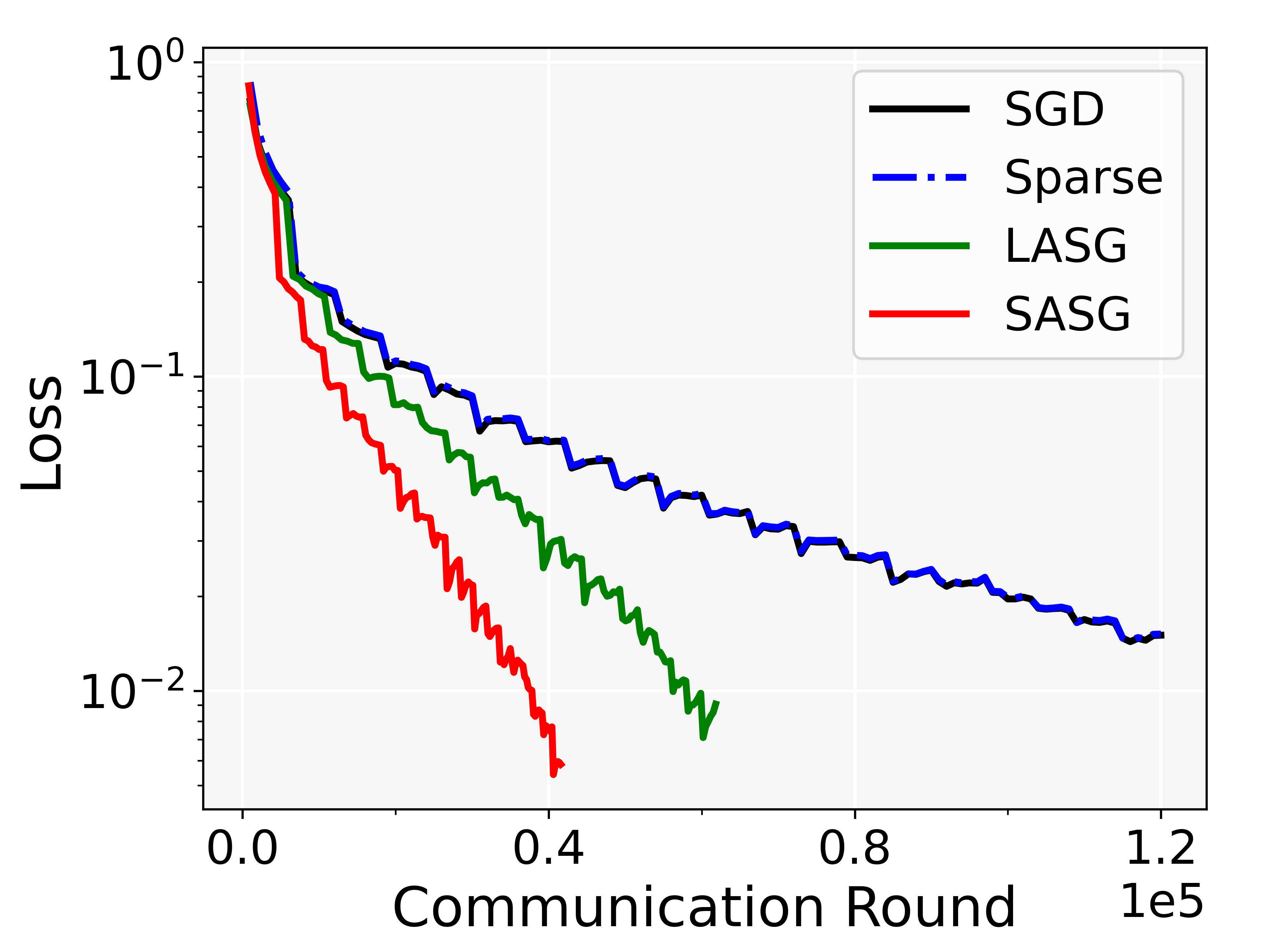
(a) FC+MNIST

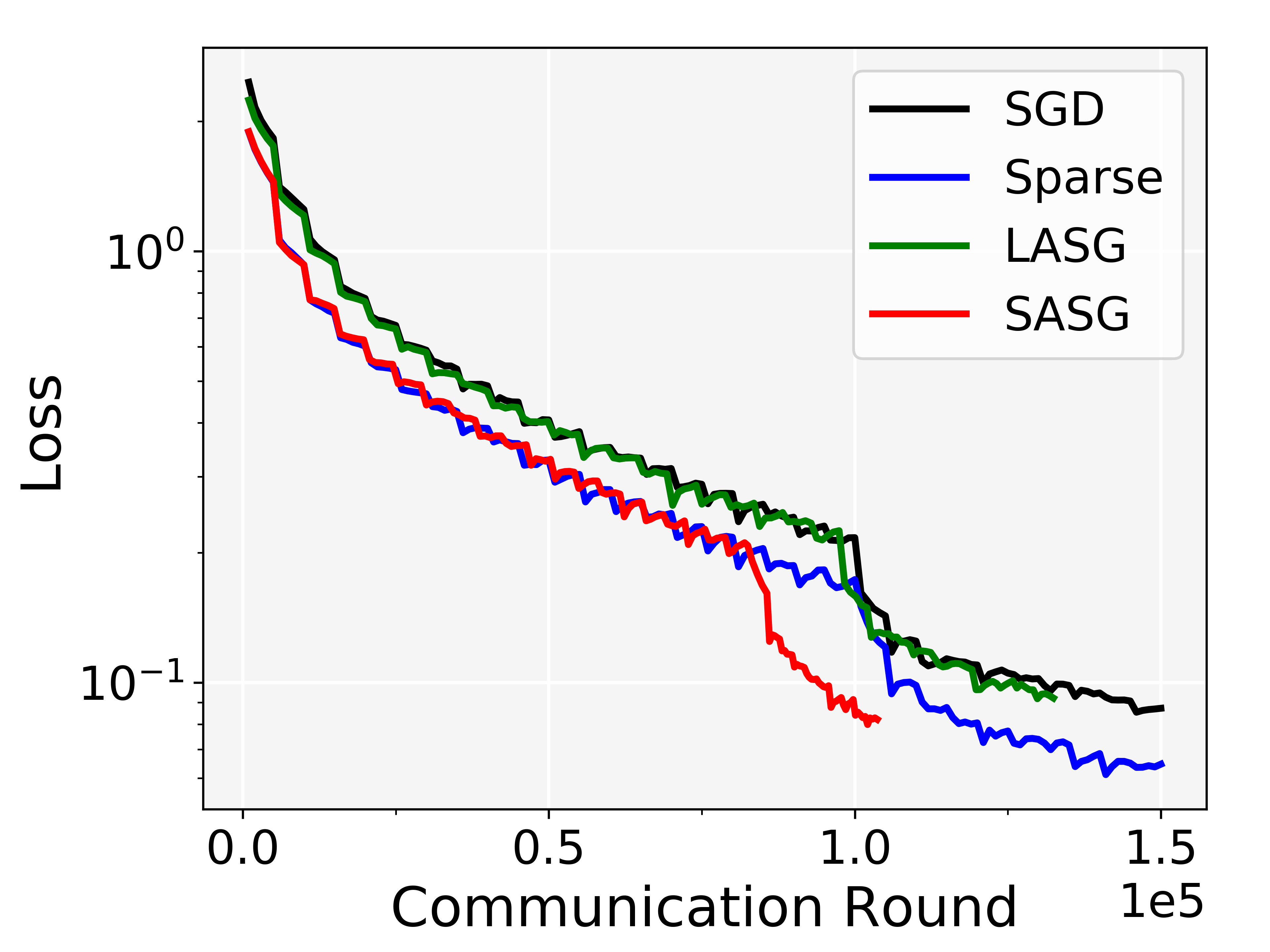
(b) ResNet18+CIFAR-10

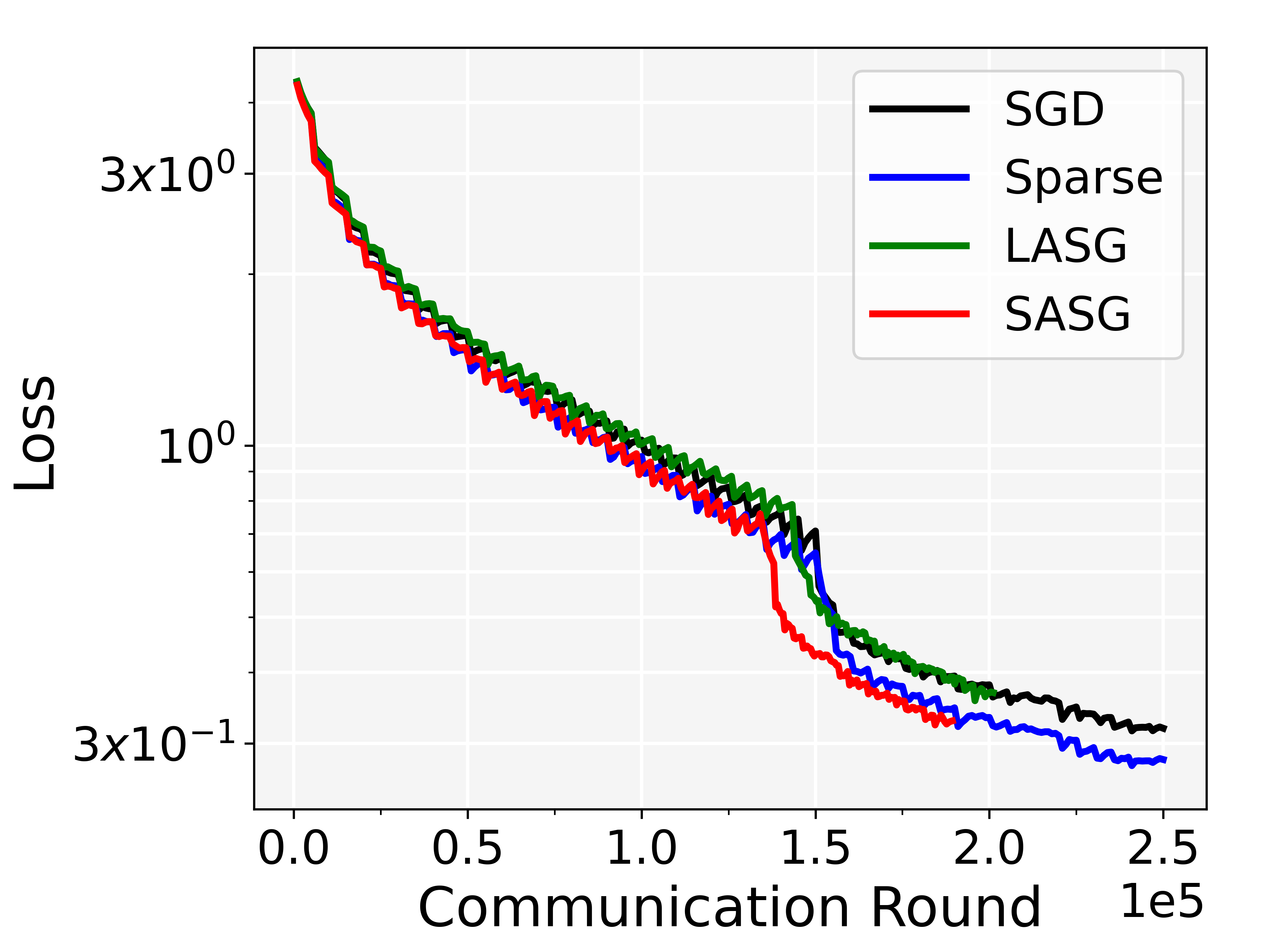
(c) ResNet18+CIFAR-100

Figure 3: Experimental results of training loss versus communication round in three settings.

MNIST: The MNIST [42] dataset contains 70,000 handwritten digits in 10 classes, with 60,000 examples in the training set and 10,000 examples in the test set. We consider a two-layer fully connected (FC) neural network model with 512 neurons in the second layer for 10-category classification on MNIST. For all algorithms, we trained $20$ epochs with the learning rate $\gamma=0.005$. For the adaptive aggregated algorithms SASG and LASG, we set $D=10,\alpha_{d}=1/2\gamma$ for $d=1,2,\ldots,10$.

CIFAR-10: The CIFAR-10 [43] dataset comprises 60,000 colored images in 10 classes, with 6,000 images per category. We test ResNet18 [44] with all the algorithms mentioned above on the CIFAR-10 dataset. Standard data augmentation techniques such as random cropping, flipping, and normalization are performed. We trained $30$ epochs for the four algorithms, and the basic learning rate is set to $\gamma=0.01$, with a learning rate decay of $0.1$ at epoch $20$. For SASG and LASG, we set $D=10,\alpha_{d}=1/\gamma$ for $d=1,2,\ldots,10$.

CIFAR-100: We also test ResNet18 on the CIFAR-100 [43] dataset, which consists of 60,000 images in 100 classes. A data augmentation technique similar to CIFAR-10 was performed. The basic learning rate is set to $\gamma=0.01$, with a learning rate decay of $0.1$ at epoch $30$, where the total training epoch is $50$. For SASG and LASG, we set $D=10,\alpha_{d}=1/\gamma$ for $d=1,2,\ldots,10$.

Note also that we did not use training techniques like warm-up as well as weight decay in our experiments, and thus state-of-the-art performance was not achieved in some models. Our aim is to verify through comparative experiments that the SASG algorithm can reduce both the number of communication rounds and bits without sacrificing model performance.

5.2 Communication Volume

Model & Dataset	Method	# Rounds	# Bits
FC MNIST	SGD	63200	8.23 E+11
	Sparse	66600	8.68 E+09
	LASG	37129	4.84 E+11
	SASG	22721	2.96 E+09
ResNet18 CIFAR-10	SGD	112200	4.01 E+13
	Sparse	112800	4.03 E+11
	LASG	110227	3.94 E+13
	SASG	90214	3.23 E+11
ResNet18 CIFAR-100	SGD	151600	5.44 E+13
	Sparse	153000	5.49 E+11
	LASG	145886	5.24 E+13
	SASG	138119	4.96 E+11

TABLE II: Number of communication rounds and bits required for the four algorithms to reach the same test accuracy baseline (average of five experiments).

This part will give the simulation experiment results on the communication volume, i.e., the number of communication rounds and bits. Test accuracy and training loss versus the number of communication rounds are reported in Figures 2-3, where Figure 2(c) plots the top-5 test accuracy.

The results in Figure 2 show that our SASG algorithm is more efficient than the previous methods. For example, in Figure 2(a), SASG can obtain higher test accuracy using the same number of communication rounds, implying that our algorithm picks out the more meaningful rounds for communication. Moreover, after completing the training process, SASG can significantly reduce the number of communication rounds while achieving the same performance. Figure 3 gives the experimental results of the training loss versus the number of communication rounds. In Figure 3(a) (training on the MNIST dataset), we can see that the SASG algorithm achieves faster and better convergence results with fewer communication rounds. In the experiments on the CIFAR-10 and CIFAR-100 datasets (Figure 3(b)-3(c)), SASG is also able to significantly reduce the number of communication rounds required to complete the training while guaranteeing convergence.

We choose several baselines to present the specific number of communication rounds and bits required to achieve the same performance for the four algorithms, with the accuracy baseline set as 98% for MNIST, 92% for CIFAR-10 and CIFAR-100 (top-5 accuracy), respectively. As shown in Table II, thanks to the adaptive aggregation technique, both SASG and LASG algorithms reduce the number of communication rounds, while our SASG algorithm is more effective. The number of communication bits required by the different algorithms to reach the same baseline can be obtained by calculating the number of parameters for different models. The last column of Table II shows that the SASG algorithm combining adaptive aggregation techniques and sparse communication outperforms the LASG and sparsification methods, significantly reducing the number of communication bits required for the model to achieve the same performance.

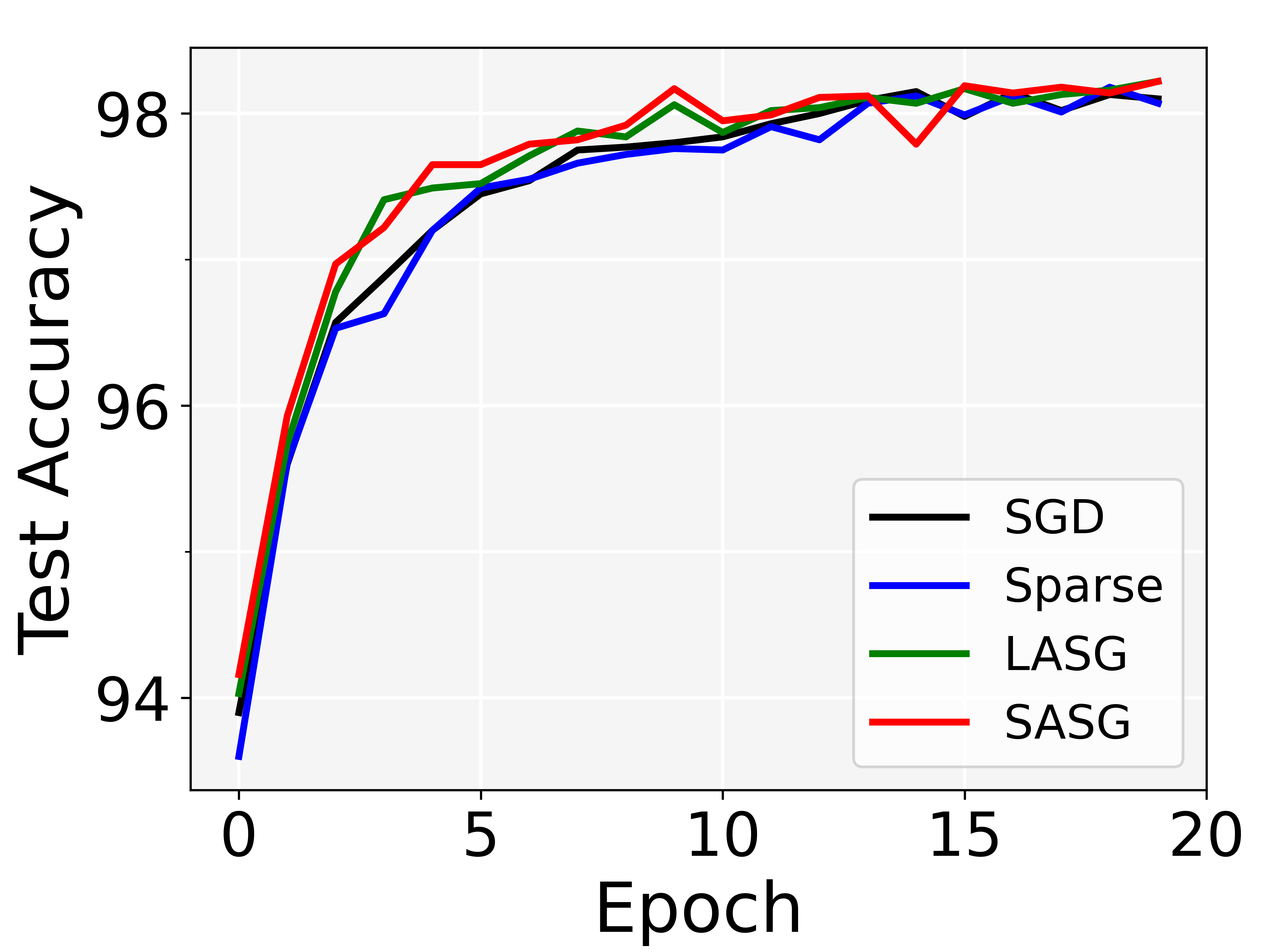
(a) Accuracy v.s. Epoch

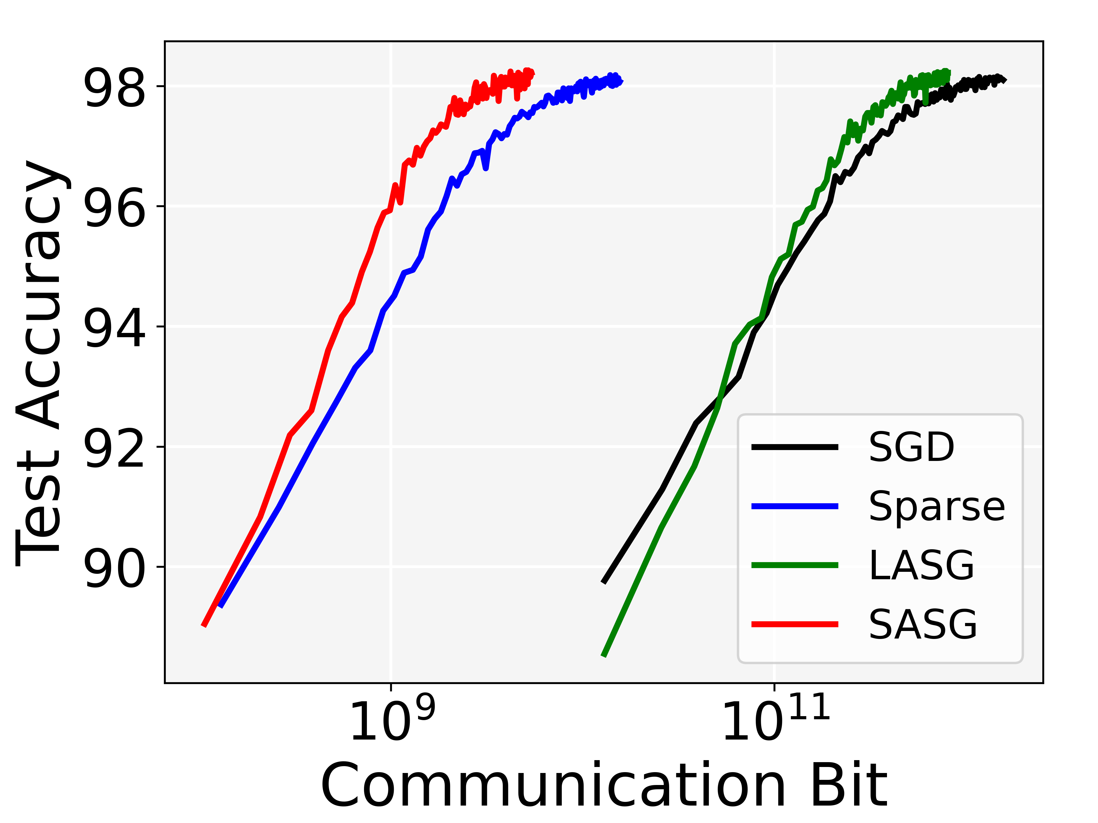
(b) Accuracy v.s. Bit

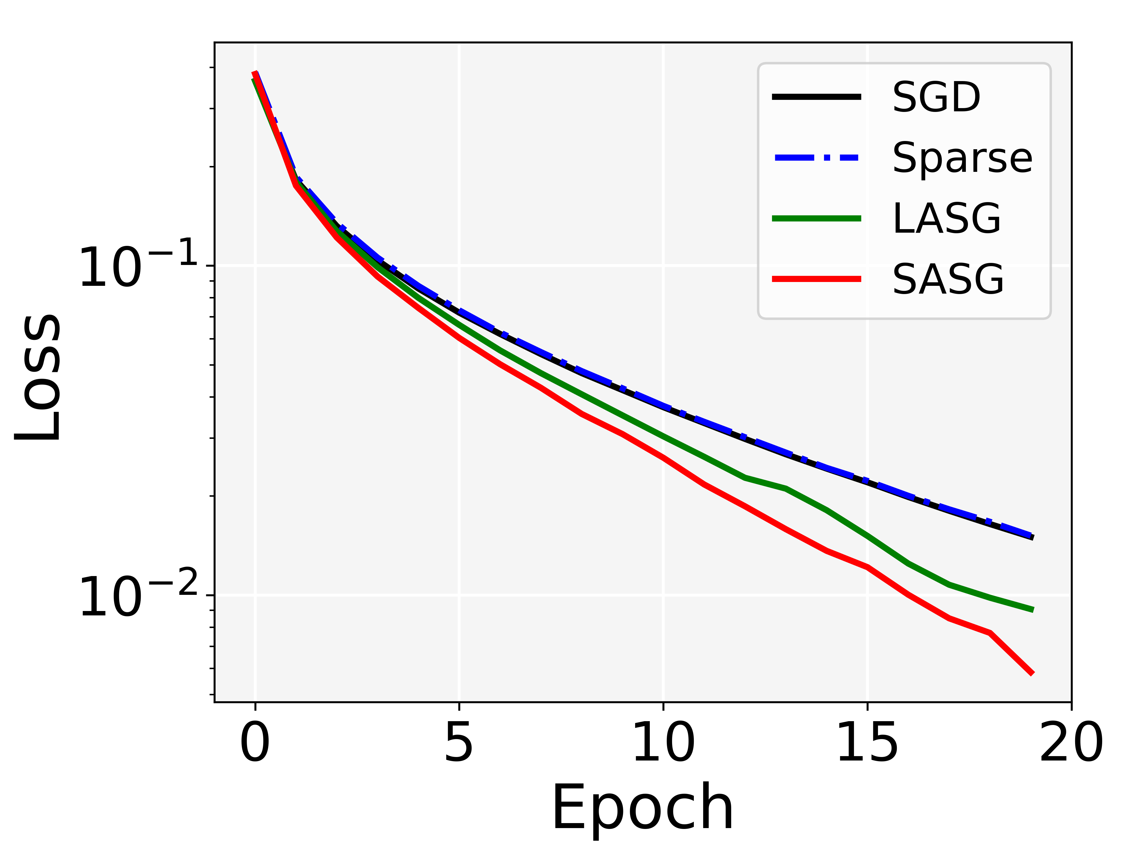
(c) Loss v.s. Epoch

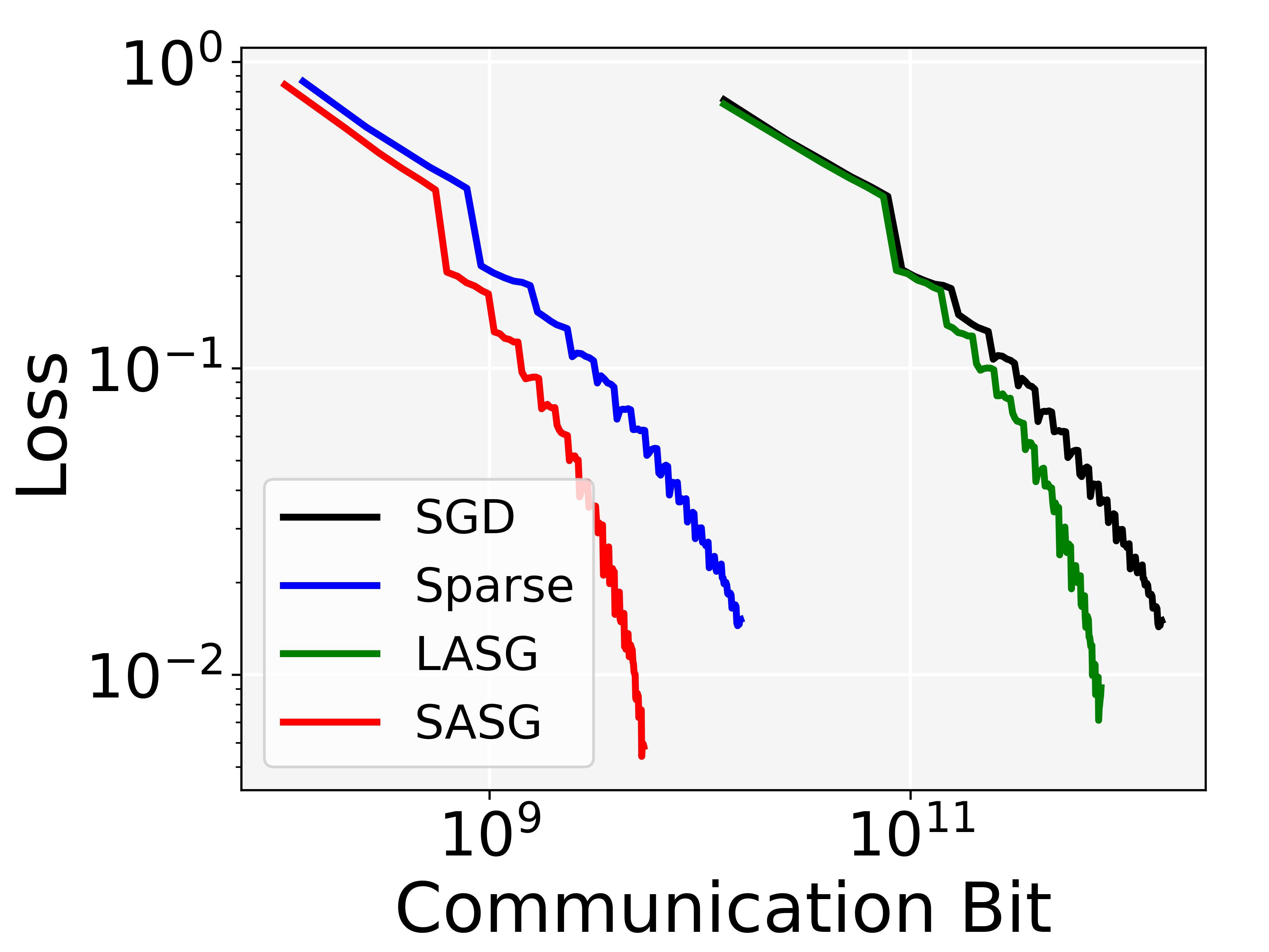
(d) Loss v.s. Bit

Figure 4: Experimental results of test accuracy and training loss versus epoch and communication bit (fully-connected neural network).

We also plot the test accuracy and training loss versus the training epochs and the number of communication bits. The results on training epochs (Figures 4(a), 4(c)) show that the SASG algorithm is convergent with the same rate as SGD, which is consistent with our theoretical results. The remaining experimental results (Figures 4(b), 4(d)) show that our algorithm can significantly reduce the number of communication bits.

5.3 Communication Time

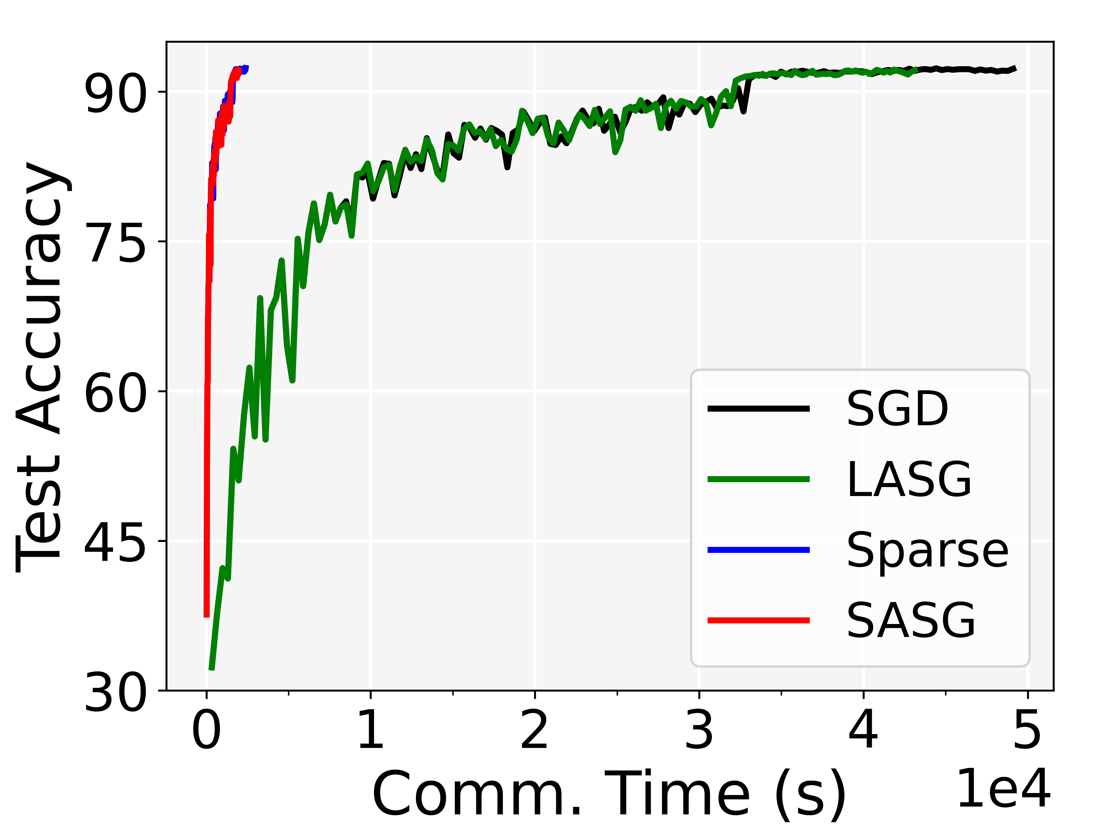
(a) Accuracy v.s. Time

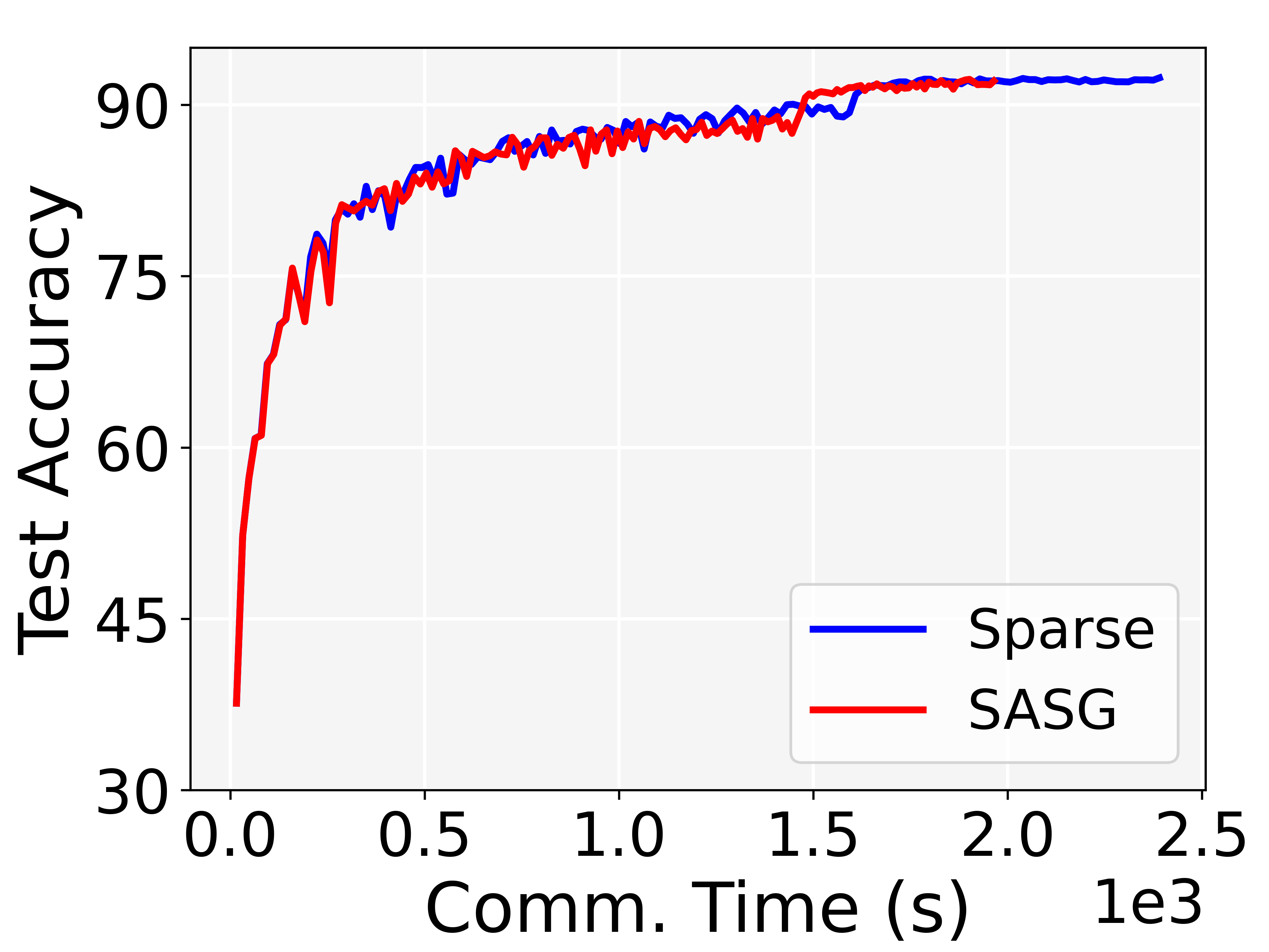
(b) Accuracy v.s. Time

Figure 5: Experimental results of test accuracy versus communication time (ResNet18+Cifar10).

This part will present the communication time required for each algorithm to perform distributed training. As we mentioned in Section 3, the top-$k$ sparsification method can significantly reduce the number of communication bits. Thus the sparsification method and the SASG algorithm require much less communication time than the LASG and SGD algorithms when completing the same training task, as shown in Figure 5(a). The two methods using the sparsification technique are compared in Figure 5(b), showing that our SASG algorithm is more efficient. Specifically, the SASG algorithm achieves the required accuracy faster and completes training in less communication time.

Figure 6 recorded the communication time required by the sparsification method and the SASG algorithm for every $100$ training iterations. As training proceeds, SASG skips more communication rounds and the required communication time gradually decreases, while the sparsification method remains the same. In addition, it can be seen from Figure 5(b) that skipping this redundant information does not harm the final performance of the model, which also indicates that our adaptive selection criterion is effective. The average communication time is shown in Table III.

Method	Communication	Computation	Memory
SGD	327.45s	—	—
Sparse	15.94s	—	—
LASG	286.72s	1.25s	426.25MB
SASG	13.09s	1.25s	4.26MB

TABLE III: Average communication time of the four algorithms and extra overhead required for the two adaptive aggregated methods (record every 100 training iterations).

Finally, we also need to discuss the additional overhead required to execute the SASG algorithm, i.e., the extra computation time for calculating the selection rule and the memory overhead required for storing the stale gradients. As seen in Algorithm 1, in one SASG iteration, each worker needs to store one copy of the old model parameters to compute the auxiliary gradient, and the server needs to store the old gradient (sparse one) from each worker. Table III presents the additional overhead required for the two adaptive aggregated methods. The computational overhead is approximately the same for both methods, mainly for computing an auxiliary gradient, but this overhead is small compared to the communication time. On the other hand, the SASG algorithm only needs to store the sparsified gradients on the server-side compared to the LASG algorithm, so it can significantly reduce the additional memory overhead.

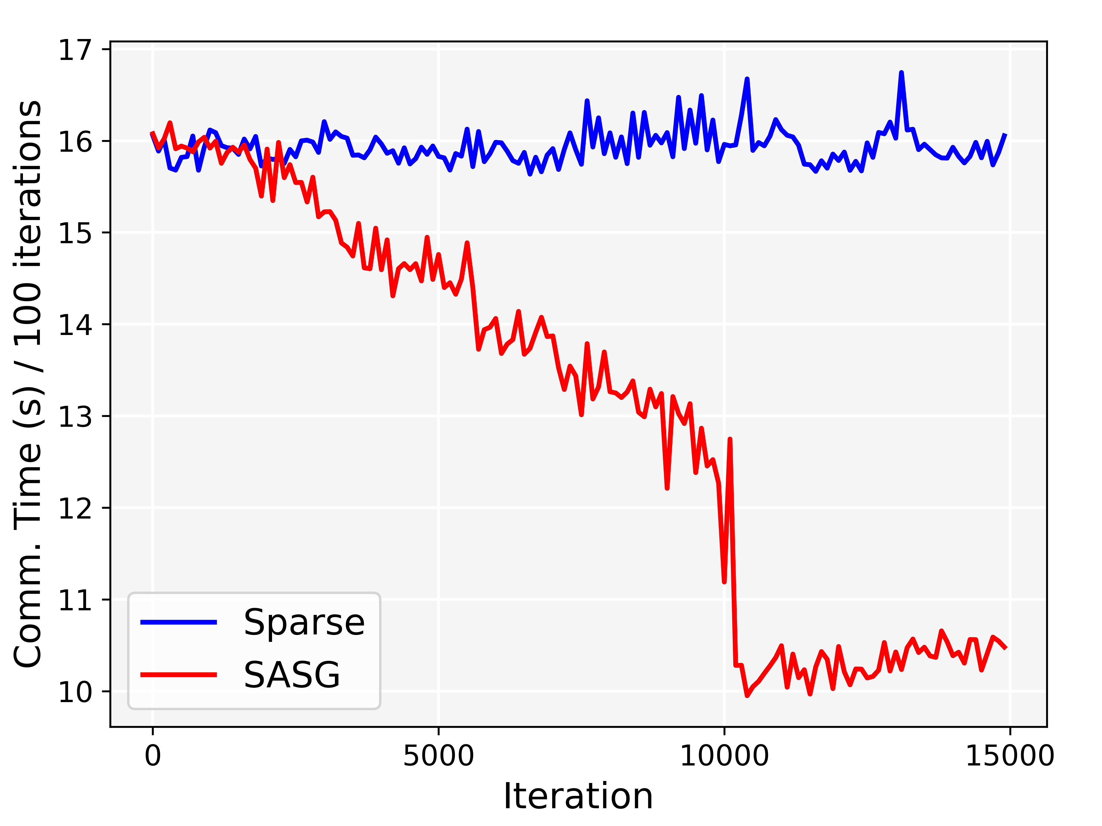
Figure 6: Experimental results of communication time versus training iteration (recorded every $100$ iterations). Learning rate decay was used at the $10,000$-th iteration.

6 Proofs

The section contains proof details of lemmas and the theorem in Section 4. All the theoretical proofs are based on the standard Assumptions 1, 2, and 3.

6.1 Proof of Lemma 1

Given a vector $\mathbf{x}\in\mathbb{R}^{d}$, from Definition 1, we can see that only the first $k$ largest coordinates of the vector are retained. That is

$$\|\mathcal{T}_{k}(\mathbf{x})\|^{2}\geq\frac{k}{d}\|\mathbf{x}\|^{2}.$$

Due to that $\left\langle\mathcal{T}_{k}(\mathbf{x})-\mathbf{x},\mathcal{T}_{k}(\mathbf{x})\right\rangle=0$,

$$\|\mathcal{T}_{k}(\mathbf{x})-\mathbf{x}\|^{2}=\|\mathbf{x}\|^{2}-\|\mathcal{T}_{k}(\mathbf{x})\|^{2}.$$

With $\delta:=k/d\in(0,1)$, we further conclude that

$$\|\mathcal{T}_{k}(\mathbf{x})-\mathbf{x}\|^{2}\leq(1-\delta)\|\mathbf{x}\|^{2}.$$

$\blacksquare$

6.2 Proof of Lemma 2

From Algorithm 1 and Lemma 1, we can see that

$$\begin{split}&\mathbb{E}[\|{e}_{m}^{t+1}\|^{2}]=\mathbb{E}[\|{g}_{m}^{t}-\mathcal{T}_{k}({g}_{m}^{t})\|^{2}]\leq(1-\delta)\mathbb{E}[\|{g}_{m}^{t}\|^{2}]\\ &=(1-\delta)\mathbb{E}\left[\|\gamma\nabla f_{m}({\omega}^{t},\xi_{m}^{t})+{e}_{m}^{t}\|^{2}\right]\\ &\leq(1-\delta)\Big{(}(1+\eta)\mathbb{E}\|{e}_{m}^{t}\|^{2}+(1+\frac{1}{\eta})\gamma^{2}\mathbb{E}\|\nabla f_{m}({\omega}^{t},\xi_{m}^{t})\|^{2}\Big{)}\end{split}$$

where we used Young’s inequality (for any $\eta>0$). From Algorithm 1 and Assumption 3, we have that ${e}_{m}^{0}=0$ and $\nabla f_{m}({\omega}^{t},\xi_{m}^{t})$ is bounded. A simple calculation yields

$$\begin{split}&\mathbb{E}[\|{e}_{m}^{t+1}\|^{2}]\\ &\leq\sum_{l=0}^{t}\big{[}(1-\delta)(1+\eta)\big{]}^{t-l}(1-\delta)(1+\frac{1}{\eta})\gamma^{2}\mathbb{E}\|\nabla f_{m}({\omega}^{l},\xi_{m}^{l})\|^{2}\\ &\leq\sum_{l=0}^{\infty}\big{[}(1-\delta)(1+\eta)\big{]}^{l}(1-\delta)(1+\frac{1}{\eta})\gamma^{2}B_{m}^{2}\\ &=\frac{(1-\delta)(1+1/\eta)}{1-(1-\delta)(1+\eta)}\gamma^{2}B_{m}^{2}.\end{split}$$

Let us pick $\eta:=\frac{\delta}{2(1-\delta)}$, then we have

$$\mathbb{E}[\|{e}_{m}^{t+1}\|^{2}]\leq\frac{2(1-\delta)(1+1/\eta)}{\delta}\gamma^{2}B_{m}^{2}\leq\frac{4(1-\delta)}{\delta^{2}}\gamma^{2}B_{m}^{2}.$$

$\blacksquare$

6.3 Proof of Equation (10)

Following Definition 2 and the iterative scheme (8), we have

$$\begin{split}&\nu^{t+1}=\omega^{t+1}-\frac{1}{M}\sum_{m\in\mathcal{M}}e_{m}^{t+1}\\ &=\omega^{t}-\frac{1}{M}\left[\sum_{m\in\mathcal{M}^{t}}\mathcal{T}_{k}(g_{m}^{t})+\sum_{m\in\mathcal{M}_{c}^{t}}\mathcal{T}_{k}(g_{m}^{t-\tau_{m}^{t}})+\sum_{m\in\mathcal{M}}e_{m}^{t+1}\right]\\ &\overset{*}{=}\omega^{t}-\frac{1}{M}\left[\sum_{m\in\mathcal{M}^{t}}g_{m}^{t}+\sum_{m\in\mathcal{M}_{c}^{t}}g_{m}^{t-\tau_{m}^{t}}\right]\\ &=\omega^{t}-\frac{1}{M}\sum_{m\in\mathcal{M}^{t}}\left(\gamma\nabla f_{m}({\omega}^{t};\xi_{m}^{t})+e_{m}^{t}\right)\\ &\quad-\frac{1}{M}\sum_{m\in\mathcal{M}_{c}^{t}}\left(\gamma\nabla f_{m}({\omega}^{t-\tau_{m}^{t}};\xi_{m}^{t-\tau_{m}^{t}})+e_{m}^{t-\tau_{m}^{t}}\right)\\ &\overset{*}{=}\nu^{t}-\frac{\gamma}{M}\sum_{m\in\mathcal{M}}\nabla f_{m}({\omega}^{t};\xi_{m}^{t})\\ &\quad+\frac{\gamma}{M}\sum_{m\in\mathcal{M}_{c}^{t}}\left(\nabla f_{m}({\omega}^{t};\xi_{m}^{t})-\nabla f_{m}({\omega}^{t-\tau_{m}^{t}};\xi_{m}^{t-\tau_{m}^{t}})\right),\end{split}$$

where $(*)$ used $e_{m}^{t+1}=e_{m}^{t-\tau_{m}^{t}},\forall m\in\mathcal{M}_{c}^{t}$. Let

$$\Delta_{m}^{t}:=\nabla f_{m}({\omega}^{t};\xi_{m}^{t})-\nabla f_{m}({\omega}^{t-\tau_{m}^{t}};\xi_{m}^{t-\tau_{m}^{t}}),$$

then we have that

$$\nu^{t+1}-\nu^{t}=-\frac{\gamma}{M}\sum_{m\in\mathcal{M}}\nabla f_{m}({\omega}^{t};\xi_{m}^{t})+\frac{\gamma}{M}\sum_{m\in\mathcal{M}_{c}^{t}}\Delta_{m}^{t}.$$ (13)

$\blacksquare$

6.4 Proof of Lemma 3

We first give the whole analysis process and then explain the relevant details.

$$\begin{split}&\mathbb{E}\left[F(\nu^{t+1})\right]-\mathbb{E}\left[F(\nu^{t})\right]\\ &\overset{(a)}{\leq}\mathbb{E}\left\langle\nabla F(\nu^{t}),\nu^{t+1}-\nu^{t}\right\rangle+\frac{L}{2}\mathbb{E}\|\nu^{t+1}-\nu^{t}\|^{2}\\ &\overset{(b)}{\leq}\mathbb{E}\left\langle\nabla F({\omega}^{t}),-\frac{\gamma}{M}\sum_{m\in\mathcal{M}}\nabla f_{m}({\omega}^{t};\xi_{m}^{t})+\frac{\gamma}{M}\sum_{m\in\mathcal{M}_{c}^{t}}\Delta_{m}^{t}\right\rangle\\ &\quad+\mathbb{E}\left\langle\nabla F(\nu^{t})-\nabla F(\omega^{t}),\nu^{t+1}-\nu^{t}\right\rangle+\frac{L}{2}\mathbb{E}\|\nu^{t+1}-\nu^{t}\|^{2}\\ &\overset{(c)}{\leq}-\frac{\gamma}{M}\mathbb{E}\|\nabla F({\omega}^{t})\|^{2}+\frac{\gamma}{M}\mathbb{E}\left\langle\nabla F({\omega}^{t}),\sum_{m\in\mathcal{M}_{c}^{t}}\Delta_{m}^{t}\right\rangle\\ &\quad+\frac{1}{2}\mathbb{E}\|\nabla F(\nu^{t})-\nabla F({\omega}^{t})\|^{2}+\frac{L+1}{2}\mathbb{E}\|\nu^{t+1}-\nu^{t}\|^{2}\\ &\overset{(d)}{\leq}-(\gamma-\frac{L\gamma^{2}}{2})\cdot\frac{1}{M}\mathbb{E}\|\nabla F({\omega}^{t})\|^{2}+\frac{L+1}{2}\mathbb{E}\|\nu^{t+1}-\nu^{t}\|^{2}\\ &\quad+\sum_{d=1}^{D}\left[\frac{\alpha_{d}}{2ML}+\frac{L}{2}\right]\|\omega^{t+1-d}-\omega^{t-d}\|^{2}\\ &\quad+\frac{L^{2}}{2}\mathbb{E}\left[\|\nu^{t}-\omega^{t}\|^{2}\right]+\frac{\gamma^{2}DL\sigma^{2}}{M}\end{split}$$

$$\begin{split}&\overset{(e)}{\leq}-(\gamma-\frac{5L+4}{2}\gamma^{2})\cdot\frac{1}{M}\mathbb{E}\left[\|\nabla F({\omega}^{t})\|^{2}\right]\\ &\quad+\sum_{d=1}^{D}\left[\frac{\alpha_{d}}{2ML}+\frac{L}{2}+\frac{2\gamma^{2}(L+1)\alpha_{d}}{M^{2}}\right]\|\omega^{t+1-d}-\omega^{t-d}\|^{2}\\ &\quad+\frac{L^{2}}{2M^{2}}\mathbb{E}\left[\Big{\|}\sum_{m\in\mathcal{M}}e_{m}^{t}\Big{\|}^{2}\right]+\left[10(L+1)+DL\right]\frac{\gamma^{2}\sigma^{2}}{M},\end{split}$$ (14)

where $(a)$ uses the $L$-smooth property in Assumption 1, i.e.,$\forall\mathbf{x},\mathbf{y}\in\mathbb{R}^{d}$,

$$F(\mathbf{y})-F(\mathbf{x})\leq\left\langle\nabla F(\mathbf{x}),\mathbf{y}-\mathbf{x}\right\rangle+\frac{L}{2}\|\mathbf{y}-\mathbf{x}\|^{2}.$$

$(b)$ is obtained from equation (13). $(c)$ uses Assumption 2 and the inequality $\|a\|^{2}+\|b\|^{2}\geq 2\left\langle a,b\right\rangle$. In order to get $(d)$, we need to bound $\left\langle\nabla F(\omega^{t}),\Delta_{m}^{t}\right\rangle$ as follows

$$\begin{split}&\mathbb{E}\left\langle\nabla F(\omega^{t}),\Delta_{m}^{t}\right\rangle\\ &=\mathbb{E}\left\langle\nabla F(\omega^{t}),\nabla f_{m}({\omega}^{t};\xi_{m}^{t})-\nabla f_{m}({\omega}^{t-\tau_{m}^{t}};\xi_{m}^{t-\tau_{m}^{t}})\right\rangle\\ &=\underbrace{\mathbb{E}\left\langle\nabla F(\omega^{t}),\nabla f_{m}({\omega}^{t};\xi_{m}^{t})-\nabla f_{m}({\omega}^{t-\tau_{m}^{t}};\xi_{m}^{t})\right\rangle}_{I}\\ &\quad+\underbrace{\mathbb{E}\left\langle\nabla F(\omega^{t}),\nabla f_{m}({\omega}^{t-\tau_{m}^{t}};\xi_{m}^{t})-\nabla f_{m}({\omega}^{t-\tau_{m}^{t}};\xi_{m}^{t-\tau_{m}^{t}})\right\rangle}_{II}.\end{split}$$

Using the inequality $\langle a,b\rangle\leq\frac{\varepsilon}{2}\|a\|^{2}+\frac{1}{2\varepsilon}\|b\|^{2}$ (with $\varepsilon:=L\gamma$) and selection rule (6), we have

$$I\leq\frac{L\gamma}{2}\mathbb{E}[\|\nabla F(\omega^{t})\|^{2}]+\frac{1}{2L\gamma}\frac{1}{M^{2}}\sum_{d=1}^{D}\alpha_{d}\|\omega^{t+1-d}-\omega^{t-d}\|^{2}.$$

Noticed that

$$\begin{split}\mathbb{E}\left\langle\nabla F(\omega^{t-\tau_{m}^{t}}),\nabla f_{m}({\omega}^{t-\tau_{m}^{t}};\xi_{m}^{t})-\nabla f_{m}({\omega}^{t-\tau_{m}^{t}};\xi_{m}^{t-\tau_{m}^{t}})\right\rangle=0\end{split}$$

we have

$$\begin{split}&II=\mathbb{E}\Big{\langle}\nabla F(\omega^{t})-\nabla F(\omega^{t-\tau_{m}^{t}}),\\ &\qquad\qquad\nabla f_{m}({\omega}^{t-\tau_{m}^{t}};\xi_{m}^{t})-\nabla f_{m}({\omega}^{t-\tau_{m}^{t}};\xi_{m}^{t-\tau_{m}^{t}})\Big{\rangle}\\ &\leq L\mathbb{E}\left\langle\omega^{t}-\omega^{t-\tau_{m}^{t}},\nabla f_{m}({\omega}^{t-\tau_{m}^{t}};\xi_{m}^{t})-\nabla f_{m}({\omega}^{t-\tau_{m}^{t}};\xi_{m}^{t-\tau_{m}^{t}})\right\rangle\\ &\leq\frac{\gamma DL}{2}\mathbb{E}\left[\|\nabla f_{m}({\omega}^{t-\tau_{m}^{t}};\xi_{m}^{t})-\nabla f_{m}({\omega}^{t-\tau_{m}^{t}};\xi_{m}^{t-\tau_{m}^{t}})\|^{2}\right]\\ &\quad+\frac{L}{2\gamma D}\|\omega^{t}-\omega^{t-\tau_{m}^{t}}\|^{2}\\ &\leq 2\gamma DL\sigma_{m}^{2}+\frac{L}{2\gamma}\sum_{d=1}^{D}\|\omega^{t+1-d}-\omega^{t-d}\|^{2},\end{split}$$

where we use the inequality $\langle a+b\rangle\leq\frac{\varepsilon}{2}\|a\|^{2}+\frac{1}{2\varepsilon}\|b\|^{2}$ (with $\varepsilon:=D\gamma$), $\|\sum_{i=1}^{n}\theta_{i}\|^{2}\leq n\sum_{i=1}^{n}\|\theta_{i}\|^{2}$, and Assumption 2. That is (with $\sigma^{2}:=\sum_{m=1}^{M}\sigma_{m}^{2}$)

$$\begin{split}&\frac{\gamma}{M}\mathbb{E}\left\langle\nabla F(\omega^{t}),\sum_{m\in\mathcal{M}_{c}^{t}}\Delta_{m}^{t}\right\rangle\leq\frac{\gamma}{M}\sum_{m\in\mathcal{M}_{c}^{t}}\left(I+II\right)\\ &\leq\frac{L\gamma^{2}}{2}\mathbb{E}[\|\nabla F(\omega^{t})\|^{2}]+\sum_{d=1}^{D}(\frac{\alpha_{d}}{2M^{2}L}+\frac{L}{2})\|\omega^{t+1-d}-\omega^{t-d}\|^{2}\\ &\quad+\frac{2\gamma^{2}DL\sigma^{2}}{M}.\end{split}$$

Further analyzing $\|\Delta_{m}^{t}\|^{2}$ and $\|\nu^{t+1}-\nu^{t}\|^{2}$, we can get $(e)$

$$\begin{split}&\|\sum_{m\in\mathcal{M}_{c}^{t}}\Delta_{m}^{t}\|^{2}\leq|\mathcal{M}_{c}^{t}|\sum_{m\in\mathcal{M}_{c}^{t}}\|\Delta_{m}^{t}\|^{2}\\ &\leq|\mathcal{M}_{c}^{t}|\sum_{m\in\mathcal{M}_{c}^{t}}\Big{\|}\nabla f_{m}({\omega}^{t};\xi_{m}^{t})-\nabla f_{m}({\omega}^{t-\tau_{m}^{t}};\xi_{m}^{t})\\ &\quad+\nabla f_{m}({\omega}^{t-\tau_{m}^{t}};\xi_{m}^{t})-\nabla f_{m}({\omega}^{t-\tau_{m}^{t}};\xi_{m}^{t-\tau_{m}^{t}})\Big{\|}^{2}\\ &\leq 2M\sum_{m\in\mathcal{M}_{c}^{t}}\|\nabla f_{m}({\omega}^{t};\xi_{m}^{t})-\nabla f_{m}({\omega}^{t-\tau_{m}^{t}};\xi_{m}^{t})\|^{2}\\ &\quad+2M\sum_{m\in\mathcal{M}_{c}^{t}}\|\nabla f_{m}({\omega}^{t-\tau_{m}^{t}};\xi_{m}^{t})-\nabla f_{m}({\omega}^{t-\tau_{m}^{t}};\xi_{m}^{t-\tau_{m}^{t}})\|^{2}\\ &\leq 2\sum_{d=1}^{D}\alpha_{d}\left\|\omega^{t+1-d}-\omega^{t-d}\right\|^{2}+8M\sigma^{2},\end{split}$$ (15)

where $\sigma^{2}:=\sum_{m=1}^{M}\sigma_{m}^{2}$. Then, using (13), (15) and Assumption 2, we can get

$$\begin{split}&\mathbb{E}[\|\nu^{t+1}-\nu^{t}]\|^{2}\\ &=\mathbb{E}[\|-\frac{\gamma}{M}\sum_{m\in\mathcal{M}}\nabla f_{m}({\omega}^{t};\xi_{m}^{t})+\frac{\gamma}{M}\sum_{m\in\mathcal{M}_{c}^{t}}\Delta_{m}^{t}\|^{2}]\\ &\leq\frac{2\gamma^{2}}{M^{2}}\mathbb{E}[\|\sum_{m\in\mathcal{M}}\nabla f_{m}({\omega}^{t};\xi_{m}^{t})\|^{2}]+\frac{2\gamma^{2}}{M^{2}}\mathbb{E}[\|\sum_{m\in\mathcal{M}_{c}^{t}}\Delta_{m}^{t}\|^{2}]\\ &\leq 4\gamma^{2}\mathbb{E}[\|\nabla F(\omega^{t})\|^{2}]+\frac{4\gamma^{2}}{M^{2}}\sum_{d=1}^{D}\alpha_{d}\|\omega^{t+1-d}-\omega^{t-d}\|^{2}\\ &\quad+\frac{20\gamma^{2}\sigma^{2}}{M}.\end{split}$$ (16)

Organizing and summarizing these items, we can obtain the final result (14).

$\blacksquare$

6.5 Proof of Lemma 4

According to the definition (12) and Lemma 3, a direct calculation gives

$$\begin{split}&\mathcal{L}^{t+1}-\mathcal{L}^{t}=\mathbb{E}[F(\nu^{t+1})]-\mathbb{E}[F(\nu^{t})]\\ &\quad+\sum_{d=1}^{D}\beta_{d}\|\omega^{t+2-d}-\omega^{t+1-d}\|^{2}-\sum_{d=1}^{D}\beta_{d}\|\omega^{t+1-d}-\omega^{t-d}\|^{2}\\ &\leq-(\gamma-\frac{5L+4}{2}\gamma^{2})\mathbb{E}\|\nabla F({\omega}^{t})\|^{2}+\frac{L^{2}}{2M^{2}}\mathbb{E}\|\sum_{m\in\mathcal{M}}e_{m}^{t}\|^{2}\\ &\quad+\sum_{d=1}^{D}\left[\frac{\alpha_{d}}{2M^{2}L}+\frac{L}{2}+\frac{2\gamma^{2}(L+1)\alpha_{d}}{M^{2}}\right]\|\omega^{t+1-d}-\omega^{t-d}\|^{2}\\ &\quad+\left[10(L+1)+2DL\right]\frac{\gamma^{2}\sigma^{2}}{M}+\beta_{1}\|\omega^{t+1}-\omega^{t}\|^{2}\\ &\quad+\sum_{d=1}^{D-1}(\beta_{d+1}-\beta_{d})\|\omega^{t+1-d}-\omega^{t-d}\|^{2}\\ &\quad-\beta_{D}\|\omega^{t+1-D}-\omega^{t-D}\|^{2}.\end{split}$$

Using the properties (13), (16), and Lemma 2, we can obtain the following inequality

$$\begin{split}\|\omega^{t+1}-\omega^{t}\|^{2}&\leq 2\|\nu^{t+1}-\nu^{t}\|^{2}+\frac{2}{M^{2}}\|\sum_{m\in\mathcal{M}}(e_{m}^{t+1}-e_{m}^{t})\|^{2}\\ &\leq 2\|\nu^{t+1}-\nu^{t}\|^{2}+\frac{16(1-\delta)\gamma^{2}B^{2}}{\delta^{2}M},\end{split}$$

where $B^{2}:=\sum_{m=1}^{M}B_{m}^{2}$. Then we can further get

$$\begin{split}&\mathcal{L}^{t+1}-\mathcal{L}^{t}\\ &\leq-\Big{[}\gamma-(\frac{5L+4}{2}+8\beta_{1})\gamma^{2}\Big{]}\mathbb{E}[\|\nabla F({\omega}^{t})\|^{2}]\\ &\quad-\sum_{d=1}^{D-1}\Big{[}\beta_{d}-\beta_{d+1}-\Big{(}\frac{\alpha_{d}}{2M^{2}L}+\frac{L}{2}+\frac{2\gamma^{2}(L+1)\alpha_{d}}{M^{2}}\\ &\qquad+\frac{8\beta_{1}\gamma^{2}\alpha_{d}}{M^{2}}\Big{)}\Big{]}\cdot\|\omega^{t+1-d}-\omega^{t-d}\|^{2}\\ &\quad-\left[\beta_{D}-\left(\frac{\alpha_{D}}{2M^{2}L}+\frac{L}{2}+\frac{2\gamma^{2}(L+1)\alpha_{D}}{M^{2}}+\frac{8\beta_{1}\gamma^{2}\alpha_{D}}{M^{2}}\right)\right]\\ &\qquad\cdot\|\omega^{t+1-D}-\omega^{t-D}\|^{2}\\ &\quad+\left[10(L+1)+2DL+40\beta_{1}\right]\frac{\gamma^{2}\sigma^{2}}{M}\\ &\quad+\frac{(2L^{2}+16\beta_{1})(1-\delta)}{\delta^{2}}\frac{\gamma^{2}B^{2}}{M}.\end{split}$$

For brevity, we make the following notation

$$\left\{\begin{array}[]{l}\displaystyle c_{f}:=\gamma-(\frac{5L+4}{2}+8\beta_{1})\gamma^{2}\vspace{1.0ex}\\ \displaystyle c_{d}:=\beta_{d}-\beta_{d+1}-\left(\frac{\alpha_{d}}{2M^{2}L}+\frac{L}{2}+\frac{2\gamma^{2}\alpha_{d}(L+1+4\beta_{1})}{M^{2}}\right)\vspace{1.0ex}\\ \qquad d=1,\ldots,D-1\vspace{1.1ex}\\ \displaystyle c_{D}:=\beta_{D}-\left(\frac{\alpha_{D}}{2M^{2}L}+\frac{L}{2}+\frac{2\gamma^{2}\alpha_{D}(L+1+4\beta_{1})}{M^{2}}\right)\vspace{1.1ex}\\ \displaystyle a:=10(L+1)+2DL+40\beta_{1}\vspace{1.1ex}\\ \displaystyle b:=\frac{(2L^{2}+16\beta_{1})(1-\delta)}{\delta^{2}}.\end{array}\right.$$ (17)

Eventually, we have that

$$\begin{split}&\mathcal{L}^{t+1}-\mathcal{L}^{t}\leq-\Big{[}\gamma-(\frac{5L+4}{2}+8\beta_{1})\gamma^{2}\Big{]}\mathbb{E}[\|\nabla F({\omega}^{t})\|^{2}]\\ &\qquad\qquad\quad-\sum_{d=1}^{D}c_{d}\|\omega^{t+1-d}-\omega^{t-d}\|^{2}+a\frac{\gamma^{2}\sigma^{2}}{M}+b\frac{\gamma^{2}B^{2}}{M}\\ &\leq-c_{f}\mathbb{E}[\|\nabla F({\omega}^{t})\|^{2}]-\sum_{d=1}^{D}c_{d}\|\omega^{t+1-d}-\omega^{t-d}\|^{2}\\ &\quad+a\frac{\gamma^{2}\sigma^{2}}{M}+b\frac{\gamma^{2}B^{2}}{M}.\end{split}$$

$\blacksquare$

6.6 Proof of Theorem 1

From Lemma 4, we have

$$\begin{split}\mathcal{L}^{t+1}-\mathcal{L}^{t}\leq&-c_{f}\mathbb{E}[\|\nabla F({\omega}^{t})\|^{2}]+a\frac{\gamma^{2}\sigma^{2}}{M}+b\frac{\gamma^{2}B^{2}}{M}\\ &-\sum_{d=1}^{D}c_{d}\|\omega^{t+1-d}-\omega^{t-d}\|^{2}.\end{split}$$

Let $\gamma\leq\overline{\gamma}=\frac{1}{5L+4+16\beta_{1}}$, then choose $\{\beta_{d}\}_{d=1}^{D}$ such that

$$\left\{\begin{array}[]{l}\displaystyle\beta_{d}-\beta_{d+1}-\left[\frac{\alpha_{d}}{2M^{2}L}+\frac{L}{2}+\frac{2\overline{\gamma}^{2}\alpha_{d}(L+1+4\beta_{1})}{M^{2}}\right]=0\\ \qquad d=1,\ldots,D-1\\ \displaystyle\beta_{D}-\left[\frac{\alpha_{D}}{2M^{2}L}+\frac{L}{2}+\frac{2\overline{\gamma}^{2}\alpha_{D}(L+1+4\beta_{1})}{M^{2}}\right]=0.\\ \end{array}\right.$$

Solving the linear equations above we can further get

$$\beta_{1}=\frac{[\frac{2\overline{\gamma}^{2}(L+1)}{M^{2}}+\frac{1}{2M^{2}L}]\sum_{d=1}^{D}\alpha_{d}+\frac{LD}{2}}{1-\frac{8\overline{\gamma}^{2}}{M^{2}}\sum_{d=1}^{D}\alpha_{d}}.$$

We then have $c_{d}\geq 0,d=1,\ldots,D$ and $c_{f}\geq\gamma/2$. That is

$$\mathcal{L}^{t+1}-\mathcal{L}^{t}\leq-\frac{\gamma}{2}\mathbb{E}[\|\nabla F({\omega}^{t})\|^{2}]+\frac{a\sigma^{2}+bB^{2}}{M}\gamma^{2}.$$

By taking summation $\sum\limits_{t=0}^{T-1}\mathcal{L}^{t+1}-\mathcal{L}^{t}$, we have

$$\begin{split}\sum_{t=0}^{T-1}\frac{\gamma}{2}\mathbb{E}[\|\nabla F({\omega}^{t})\|^{2}]&\leq\mathcal{L}^{0}-\mathcal{L}^{T}+\frac{a\sigma^{2}+bB^{2}}{M}T\gamma^{2}\\ &\leq F(\omega^{0})-F^{*}+\frac{a\sigma^{2}+bB^{2}}{M}T\gamma^{2}.\end{split}$$

If we choose the learning rate

$$\gamma=\min\left\{\frac{1}{5L+4+16\beta_{1}},\frac{c_{\gamma}}{\sqrt{T}}\right\},$$

where $c_{\gamma}>0$ is a constant. We then have

$$\begin{split}&\frac{1}{T}\sum_{t=0}^{T-1}\mathbb{E}\left[\|\nabla F({\omega}^{t})\|^{2}\right]\\ &\leq\frac{2M(F(\omega^{0})-F^{*})+2T(a\sigma^{2}+bB^{2})\gamma^{2}}{MT\gamma}\\ &\leq\frac{2(5L+4+16\beta_{1})(F(\omega^{0})-F^{*})}{T}+\frac{2(F(\omega^{0})-F^{*})}{c_{\gamma}\sqrt{T}}\\ &\quad+\frac{2c_{\gamma}(a\sigma^{2}+bB^{2})}{M\sqrt{T}}.\end{split}$$

That is

$$\frac{1}{T}\sum_{t=0}^{T-1}\mathbb{E}\left[\|\nabla F({\omega}^{t})\|^{2}\right]=\mathcal{O}(1/\sqrt{T}).$$

$\blacksquare$

7 Conclusion

This paper proposes a distributed algorithm with the advantages of sparse communication and adaptive aggregation stochastic gradients named SASG. The SASG algorithm adaptively skips several communication rounds with an adaptive selection rule, and further reduces the number of communication bits by sparsifying the transmitted information. For the biased nature of the top-$k$ sparsification operator, our algorithm uses an error feedback format, and we give convergence results for SASG with the help of Lyapunov analysis. Experimental results show that our approach can reduce both the number of communication rounds and bits without sacrificing convergence performance, which corroborates our theoretical findings.

References

• [1] T. B. Brown, B. Mann, N. Ryder, M. Subbiah, J. Kaplan, P. Dhariwal, A. Neelakantan, P. Shyam, G. Sastry, A. Askell, S. Agarwal, A. Herbert-Voss, G. Krueger, T. Henighan, R. Child, A. Ramesh, D. M. Ziegler, J. Wu, C. Winter, C. Hesse, M. Chen, E. Sigler, M. Litwin, S. Gray, B. Chess, J. Clark, C. Berner, S. McCandlish, A. Radford, I. Sutskever, and D. Amodei, “Language models are few-shot learners,” in Advances in Neural Information Processing Systems, vol. 33, 2020, pp. 1877–1901.
• [2] J. Deng, W. Dong, R. Socher, L.-J. Li, K. Li, and L. Fei-Fei, “Imagenet: A large-scale hierarchical image database,” in 2009 IEEE conference on computer vision and pattern recognition.   IEEE, 2009, pp. 248–255.
• [3] E. P. Xing, Q. Ho, W. Dai, J. K. Kim, J. Wei, S. Lee, X. Zheng, P. Xie, A. Kumar, and Y. Yu, “Petuum: A new platform for distributed machine learning on big data,” IEEE Transactions on Big Data, vol. 1, no. 2, pp. 49–67, 2015.
• [4] M. Li, D. G. Andersen, J. W. Park, A. J. Smola, A. Ahmed, V. Josifovski, J. Long, E. J. Shekita, and B.-Y. Su, “Scaling distributed machine learning with the parameter server,” in 11th $\{$USENIX$\}$ Symposium on Operating Systems Design and Implementation ($\{$OSDI$\}$ 14), 2014, pp. 583–598.
• [5] J. Dean, G. Corrado, R. Monga, K. Chen, M. Devin, M. Mao, M. Ranzato, A. Senior, P. Tucker, K. Yang et al., “Large scale distributed deep networks,” in Advances in Neural Information Processing Systems, 2012, pp. 1223–1231.
• [6] A. Nedic and A. Ozdaglar, “Distributed subgradient methods for multi-agent optimization,” IEEE Transactions on Automatic Control, vol. 54, no. 1, p. 48, 2009.
• [7] M. Li, D. G. Andersen, A. J. Smola, and K. Yu, “Communication efficient distributed machine learning with the parameter server,” in Advances in Neural Information Processing Systems, 2014, pp. 19–27.
• [8] M. A. Zinkevich, M. Weimer, A. Smola, and L. Li, “Parallelized stochastic gradient descent,” in Advances in Neural Information Processing Systems, vol. 23, 2010, pp. 2595–2603.
• [9] M. I. Jordan, J. D. Lee, and Y. Yang, “Communication-efficient distributed statistical inference,” Journal of the American Statistical Association, vol. 114, no. 526, pp. 668–681, 2019.
• [10] S. Shi, Q. Wang, and X. Chu, “Performance modeling and evaluation of distributed deep learning frameworks on GPUs,” in 2018 IEEE 16th Intl Conf on Dependable, Autonomic and Secure Computing, 16th Intl Conf on Pervasive Intelligence and Computing, 4th Intl Conf on Big Data Intelligence and Computing and Cyber Science and Technology Congress (DASC/PiCom/DataCom/CyberSciTech).   IEEE, 2018, pp. 949–957.
• [11] Y. Lin, S. Han, H. Mao, Y. Wang, and B. Dally, “Deep gradient compression: Reducing the communication bandwidth for distributed training,” in International Conference on Learning Representations, 2018.
• [12] M. Elibol, L. Lei, and M. I. Jordan, “Variance reduction with sparse gradients,” in International Conference on Learning Representations, 2020.
• [13] S. U. Stich, J.-B. Cordonnier, and M. Jaggi, “Sparsified SGD with memory,” in Advances in Neural Information Processing Systems, vol. 31, 2018, pp. 4447–4458.
• [14] D. Alistarh, T. Hoefler, M. Johansson, N. Konstantinov, S. Khirirat, and C. Renggli, “The convergence of sparsified gradient methods,” in Advances in Neural Information Processing Systems, vol. 31, 2018, pp. 5977–5987.
• [15] A. F. Aji and K. Heafield, “Sparse communication for distributed gradient descent,” in Proceedings of the 2017 Conference on Empirical Methods in Natural Language Processing, 2017, pp. 440–445.
• [16] T. Chen, Z. Guo, Y. Sun, and W. Yin, “CADA: Communication-adaptive distributed adam,” in International Conference on Artificial Intelligence and Statistics.   PMLR, 2021, pp. 613–621.
• [17] T. Chen, Y. Sun, and W. Yin, “Communication-adaptive stochastic gradient methods for distributed learning,” IEEE Trans. Signal Process., vol. 69, pp. 4637–4651, 2021.
• [18] T. Chen, G. Giannakis, T. Sun, and W. Yin, “LAG: Lazily aggregated gradient for communication-efficient distributed learning,” in Advances in Neural Information Processing Systems, 2018, pp. 5050–5060.
• [19] D. Basu, D. Data, C. Karakus, and S. N. Diggavi, “Qsparse-local-SGD: Distributed SGD with quantization, sparsification and local computations,” in Advances in Neural Information Processing Systems, 2019, pp. 14 668–14 679.
• [20] J. Sun, T. Chen, G. Giannakis, and Z. Yang, “Communication-efficient distributed learning via lazily aggregated quantized gradients,” in Advances in Neural Information Processing Systems, 2019, pp. 3365–3375.
• [21] W. Wen, C. Xu, F. Yan, C. Wu, Y. Wang, Y. Chen, and H. Li, “TernGrad: ternary gradients to reduce communication in distributed deep learning,” in Advances in Neural Information Processing Systems, 2017, pp. 1508–1518.
• [22] S. Horváth and P. Richtárik, “A better alternative to error feedback for communication-efficient distributed learning,” in International Conference on Learning Representations, 2021.
• [23] C. Xie, S. Zheng, S. Koyejo, I. Gupta, M. Li, and H. Lin, “CSER: Communication-efficient SGD with error reset,” in Advances in Neural Information Processing Systems, vol. 33, 2020, pp. 12 593–12 603.
• [24] C.-Y. Chen, J. Ni, S. Lu, X. Cui, P.-Y. Chen, X. Sun, N. Wang, S. Venkataramani, V. V. Srinivasan, W. Zhang, and K. Gopalakrishnan, “ScaleCom: Scalable sparsified gradient compression for communication-efficient distributed training,” in Advances in Neural Information Processing Systems, vol. 33, 2020, pp. 13 551–13 563.
• [25] W. Li, Z. Wu, T. Chen, L. Li, and Q. Ling, “Communication-censored distributed stochastic gradient descent,” IEEE Transactions on Neural Networks and Learning Systems, pp. 1–13, 2021.
• [26] S. U. Stich, “Local SGD converges fast and communicates little,” in International Conference on Learning Representations, 2019.
• [27] L. Wang, W. Wang, and B. Li, “CMFL: Mitigating communication overhead for federated learning,” in 39th IEEE International Conference on Distributed Computing Systems, ICDCS 2019.   IEEE, 2019, pp. 954–964.
• [28] T. Vogels, S. P. Karimireddy, and M. Jaggi, “PowerSGD: Practical low-rank gradient compression for distributed optimization,” in Advances in Neural Information Processing Systems, vol. 32.   Curran Associates, Inc., 2019.
• [29] H. Wang, S. Sievert, Z. Charles, S. Liu, S. Wright, and D. Papailiopoulos, “ATOMO: Communication-efficient learning via atomic sparsification,” in Advances in Neural Information Processing Systems, 2018, pp. 9872–9883.
• [30] D. Alistarh, D. Grubic, J. Li, R. Tomioka, and M. Vojnovic, “QSGD: Communication-efficient sgd via gradient quantization and encoding,” in Advances in Neural Information Processing Systems, 2017, pp. 1709–1720.
• [31] Z. Tang, S. Shi, X. Chu, W. Wang, and B. Li, “Communication-efficient distributed deep learning: A comprehensive survey,” CoRR, vol. abs/2003.06307, 2020.
• [32] J. Bernstein, Y. Wang, K. Azizzadenesheli, and A. Anandkumar, “signSGD: Compressed optimisation for non-convex problems,” in Proceedings of the 35th International Conference on Machine Learning, vol. 80.   PMLR, 2018, pp. 559–568.
• [33] F. Seide, H. Fu, J. Droppo, G. Li, and D. Yu, “1-bit stochastic gradient descent and its application to data-parallel distributed training of speech DNNs,” in Fifteenth Annual Conference of the International Speech Communication Association, 2014, pp. 1058–1062.
• [34] F. Faghri, I. Tabrizian, I. Markov, D. Alistarh, D. M. Roy, and A. Ramezani-Kebrya, “Adaptive gradient quantization for data-parallel SGD,” in Advances in Neural Information Processing Systems, vol. 33, 2020, pp. 3174–3185.
• [35] J. Wangni, J. Wang, J. Liu, and T. Zhang, “Gradient sparsification for communication-efficient distributed optimization,” in Advances in Neural Information Processing Systems, 2018, pp. 1306–1316.
• [36] S. P. Karimireddy, Q. Rebjock, S. Stich, and M. Jaggi, “Error feedback fixes signSGD and other gradient compression schemes,” in International Conference on Machine Learning, 2019, pp. 3252–3261.
• [37] A. Xu, Z. Huo, and H. Huang, “Step-ahead error feedback for distributed training with compressed gradient,” in Thirty-Fifth AAAI Conference on Artificial Intelligence, 2021, pp. 10 478–10 486.
• [38] O. Shamir, N. Srebro, and T. Zhang, “Communication-efficient distributed optimization using an approximate newton-type method,” in International Conference on Machine Learning, 2014, pp. 1000–1008.
• [39] H. Hendrikx, L. Xiao, S. Bubeck, F. R. Bach, and L. Massoulié, “Statistically preconditioned accelerated gradient method for distributed optimization,” in International Conference on Machine Learning, vol. 119.   PMLR, 2020, pp. 4203–4227.
• [40] T. Lin, S. U. Stich, K. K. Patel, and M. Jaggi, “Don’t use large mini-batches, use local SGD,” in International Conference on Learning Representations, 2019.
• [41] A. Paszke, S. Gross, F. Massa, A. Lerer, J. Bradbury, G. Chanan, T. Killeen, Z. Lin, N. Gimelshein, L. Antiga, A. Desmaison, A. Köpf, E. Yang, Z. DeVito, M. Raison, A. Tejani, S. Chilamkurthy, B. Steiner, L. Fang, J. Bai, and S. Chintala, “PyTorch: An imperative style, high-performance deep learning library,” in Advances in Neural Information Processing Systems, 2019, pp. 8024–8035.
• [42] Y. LeCun, L. Bottou, Y. Bengio, and P. Haffner, “Gradient-based learning applied to document recognition,” Proceedings of the IEEE, vol. 86, no. 11, pp. 2278–2324, 1998.
• [43] A. Krizhevsky, G. Hinton et al., “Learning multiple layers of features from tiny images,” pp. 32–33, 2009.
• [44] K. He, X. Zhang, S. Ren, and J. Sun, “Deep residual learning for image recognition,” in Proceedings of the IEEE conference on computer vision and pattern recognition, 2016, pp. 770–778.
• [45] K. Simonyan and A. Zisserman, “Very deep convolutional networks for large-scale image recognition,” in International Conference on Learning Representations, 2015.