Ground state separability and criticality in interacting many-particle systems

Abstract

We analyze exact ground state (GS) separability in general $N$ particle systems with two-site couplings. General necessary and sufficient conditions for full separability, in the form of one and two-site eigenvalue equations, are first derived. The formalism is then applied to a class of $SU(n)$-type interacting systems, where each constituent has access to $n$ local levels, and where the total number parity of each level is preserved. Explicit factorization conditions for parity-breaking GS’s are obtained, which generalize those for $XYZ$ spin systems and correspond to a fundamental GS multilevel parity transition where the lowest $2^{n-1}$ energy levels cross. We also identify a multicritical factorization point with exceptional high degeneracy proportional to $N^{n-1}$, arising when the total occupation number of each level is preserved, in which any uniform product state is an exact GS. Critical entanglement properties (like full range pairwise entanglement) are shown to emerge in the immediate vicinity of factorization. Illustrative examples are provided.

I Introduction

The ground state (GS) of strongly interacting spin systems, while normally entangled Osborne and Nielsen (2002); Vidal et al. (2003); Amico et al. (2008), can exhibit the remarkable phenomenon of factorization when a suitable magnetic field is applied Kurmann et al. (1982); Müller and Shrock (1985); Roscilde et al. (2004); Amico et al. (2006); Giampaolo et al. (2008); Rossignoli et al. (2008, 2009); Giorgi (2009); Giampaolo et al. (2009). This means that for such field, the spin system admits a completely separable exact GS, i.e. a product of single spin states, despite the presence of nonnegligible couplings between the spins and the finite value of the applied field. Moreover, such product state is not necessarily trivial, in the sense that it may break fundamental symmetries of the Hamiltonian. In this case factorization signals in finite systems a special critical point where two or more levels with definite symmetry cross and the GS becomes degenerate Rossignoli et al. (2008, 2009); Giorgi (2009); Cerezo et al. (2017); Canosa et al. (2020), allowing for such symmetry breaking exact eigenstates. The exact GS then typically undergoes in this case a transition between states with distinct symmetry as the factorization point is traversed, leading to visible effects in system observables Rossignoli et al. (2008, 2009); Cerezo et al. (2017); Canosa et al. (2020). Furthermore, critical entanglement properties emerge in the immediate vicinity Amico et al. (2006); Rossignoli et al. (2008, 2009); Cerezo et al. (2017); Canosa et al. (2020), stemming ultimately from the product nature of the closely lying eigenstate.

Most studies of GS factorization have so far been restricted to interacting spin systems (see also Rezai et al. (2010); Ciliberti et al. (2010); Campbell et al. (2013); Cerezo et al. (2015)), where factorization conditions remain analytically manageable due to the small number of parameters required to specify an individual spin state. The main aim of this work is to investigate exact GS factorization in more general interacting systems, i.e., beyond the standard $SU(2)$ spin scenario, where already the characterization of a single component state is more complex. With this goal, we first derive the necessary and sufficient conditions for factorization in the form of eigenvalue equations, either for effective pair Hamiltonians or for the mean field (MF) Hamiltonian and residual couplings.

We then apply the formalism to a general $N$-component interacting system in which each constituent has $n$ accessible local levels, such that the Hamiltonian can be expressed in terms of operators satisfying an $U(n)$ algebra. For $n=2$ it reduces to a general anisotropic $XYZ$ spin system Baxter (1971) in an applied transverse field Kurmann et al. (1982); Roscilde et al. (2004); Rossignoli et al. (2009); Cerezo et al. (2015), sharing with the latter the basic level number parity symmetry. For full range couplings it comprises schematic $SU(n)$ models employed in nuclear physics for describing collective excitations Meshkov (1971); Nuñez et al. (1985); Rossignoli and Plastino (1987), while for first neighbor couplings and special choices of parameters it reduces to the $SU(n)$ Heisenberg model, also known as Uimin-Lai-Sutherland (ULS) model Uimin (1970); Lai (1974); Sutherland (1975). The study of interacting many body systems with global $SU(n)$ symmetry has aroused great interest in recent years, becoming an active research topic that links the fields of condensed matter and atomic, molecular and optical physics Sachdev (1999); Cazalilla et al. (2009); Gorshkov et al. (2010); Cazalilla and Rey (2014); Lewenstein et al. (2012); Y. (2016). Systems possessing high dimensional symmetry can unveil exotic many body physics and are suitable for describing a wide range of non-trivial phenomena. The paradigmatic $SU(n)$ Heisenberg model Uimin (1970); Lai (1974); Sutherland (1975), first employed in solid state physics in connection with the integer quantum Hall effect Affleck (1985, 1986), played also an important role in identifying unconventional magnetic states and phases Schulz (1986); Marston and Affleck (1989); Read and Sachdev (1989, 1990); Gorshkov et al. (2010); Manmana et al. (2011); Dufour et al. (2015); Nataf and Mila (2018); Yao et al. (2019). Interest on the subject has been stimulated by the unprecedented advances in quantum control techniques, which offer the possibility of realizing strongly interacting many body systems with high symmetry in alkaline earth atomic gases in optical lattices Gorshkov et al. (2010); Cazalilla et al. (2009); Y. (2016). These platforms have also received attention in relation with high precision atomic clocks et al (2014) and quantum computation Daley et al. (2008).

The general factorization formalism is presented in section II, while its application to a general $SU(n)$-type model for $N$ components is described in III. Explicit equations for the existence of uniform parity-breaking factorized GS’s are determined, and shown to correspond to a multilevel parity transition occurring for any size $N$ and coupling range, where the GS becomes $2^{n-1}$-fold degenerate (if $N\geq n-1$). A critical factorization point with exceptionally high degeneracy (which increases with size $N$) is also identified in systems with full level number symmetry, where any uniform separable state is an exact GS. Entanglement properties in the vicinity of factorization together with signatures of factorization in small systems are as well discussed. Conclusions are drawn in IV. Appendices discuss further details including the MF approximation in the model, which admits an analytic solution in the uniform case for arbitrary $n$.

II Formalism

II.1 General factorization conditions

We consider a system described by a Hilbert space ${\cal H}=\bigotimes_{p=1}^{N}{\cal H}_{p}$, such that it can be seen as a composite of $N$ subsystems with Hilbert spaces ${\cal H}_{p}$. In this scenario we assume a general Hamiltonian containing one-site terms $h_{p}$ plus two-site interactions $V_{pq}$:

$$H = \sum_{p}h_{p}+\frac{1}{2}\sum\limits_{p\neq q}V_{pq}\,,$$ (1)

$$h_{p} = \sum\limits_{\mu}b_{\mu}^{p}o_{p}^{\mu}\,,\;\;\;\;V_{pq}=\sum\limits_{\mu,\nu}J_{\mu\nu}^{pq}o_{p}^{\mu}o_{q}^{\nu}\,,$$ (2)

where $\left\{o_{p}^{\mu}\right\}$ denotes a complete set of linearly independent operators over ${\cal H}_{p}$ and $J_{\mu\nu}^{pq}=J_{\nu\mu}^{qp}$ are the coupling strengths of the interaction between sites $p$ and $q$. In particular, any spin array with two-spin interactions in a general applied magnetic field fits into this form. We use the notation $o_{p}^{\mu}\equiv\mathbbm{1}\otimes\cdots\otimes\mathbbm{1}\otimes o_{p}^{\mu}\otimes\mathbbm{1}\otimes\cdots\otimes\mathbbm{1}$ when operators are applied to global states.

We are here interested in the conditions which ensure that a completely separable state

$$\left|\Psi\right\rangle=\bigotimes_{p}\left|\psi_{p}\right\rangle=\left|\psi_{1},\ldots,\psi_{N}\right\rangle\,,$$ (3)

possibly breaking some fundamental symmetry of $H$, is an exact eigenstate of $H$:

$$H\left|\Psi\right\rangle=E\left|\Psi\right\rangle.$$ (4)

When applied to $|\Psi\rangle$, $H$ can just connect it with itself and with superpositions of one- and two-site “excitations”,

$$\left|\Phi_{p}\right\rangle = \left|\psi_{1},\ldots,\phi_{p},\ldots\psi_{N}\right\rangle\,,$$ (5)

$$\left|\Phi_{pq}\right\rangle = \left|\psi_{1},\ldots,\phi_{p},\ldots,\phi_{q},\ldots,\psi_{N}\right\rangle\,,$$ (6)

where $\left\langle\phi_{p}|\psi_{p}\right\rangle=\left\langle\phi_{q}|\psi_{q}\right\rangle=0$. Then Eq. (4) implies the necessary and sufficient conditions

$$\left\langle\Phi_{p}\right|H\left|\Psi\right\rangle = 0,\;\;\;p=1,\ldots,N\,,$$ (7)

$$\left\langle\Phi_{pq}\right|H\left|\Psi\right\rangle = 0,\;\;\;1\leq p<q\leq N\,,$$ (8)

to be satisfied $\forall$ $\left|\phi_{p}\right\rangle$, $\left|\phi_{q}\right\rangle$ orthogonal to $\left|\psi_{p}\right\rangle$, $\left|\psi_{q}\right\rangle$ respectively. Since

$$\left\langle\Phi_{p}\right|H\left|\Psi\right\rangle=\left\langle\phi_{p}\right|\tilde{h}_{p}\left|\psi_{p}\right\rangle\,,\;\;\tilde{h}_{p}=h_{p}+\sum_{q\neq p}v^{(q)}_{p}\,,$$ (9)

where $\tilde{h}_{p}$ is the local MF Hamiltonian at site $p$ and

$$v^{(q)}_{p} = \langle\psi_{q}|V_{pq}|\psi_{q}\rangle=\sum_{\mu,\nu}\!J_{\mu\nu}^{pq}\left\langle o_{q}^{\nu}\right\rangle o_{p}^{\mu}\,,$$ (10)

the average potential at $p$ due to the coupling with site $q$ ($\langle o^{\nu}_{q}\rangle=\langle\psi_{q}|o^{\nu}_{q}|\psi_{q}\rangle$), Eqs. (7) imply $\langle\phi_{p}|\tilde{h}_{p}|\psi_{p}\rangle=0$ $\forall$ $|\phi_{p}\rangle$ orthogonal to $|\psi_{p}\rangle$ and hence the eigenvalue equations

$$\tilde{h}_{p}\left|\psi_{p}\right\rangle=\lambda_{p}\left|\psi_{p}\right\rangle,\;\;p=1,\ldots,N.$$ (11)

As expected, each local state $\left|\psi_{p}\right\rangle$ in $\left|\Psi\right\rangle$ should be an eigenstate of the local MF Hamiltonian $\tilde{h}_{p}$ determined by the same $\left|\Psi\right\rangle$, implying self-consistency.

It is now convenient to rewrite $H$ as

$$H=\sum_{p}\tilde{h}_{p}+\frac{1}{2}\sum_{p\neq q}\tilde{V}_{pq}\,,$$ (12)

where $\tilde{V}_{pq}=V_{pq}-v_{p}^{(q)}-v_{q}^{(p)}$ is a residual coupling satisfying $\langle\Phi_{p}|\tilde{V}_{pq}|\Psi\rangle=\langle\Phi_{q}|\tilde{V}_{pq}|\Psi\rangle=0$. Then

$$\langle\Phi_{pq}|H|\Psi\rangle=\langle\phi_{p},\phi_{q}|\tilde{V}_{pq}|\psi_{p},\psi_{q}\rangle\,,$$ (13)

and Eqs. (8) together with previous property imply that $|\Psi\rangle$ should be an eigenstate of all $\tilde{V}_{pq}$:

$$\tilde{V}_{pq}|\psi_{p},\psi_{q}\rangle=\lambda_{pq}|\psi_{p},\psi_{q}\rangle\,,\;\;1\leq p<q\leq N\,,\\$$ (14)

with $\lambda_{pq}=\langle\tilde{V}_{pq}\rangle=-\langle V_{pq}\rangle$. As $\lambda_{p}=\langle h_{p}\rangle+\sum_{q\neq p}\langle V_{pq}\rangle$, the total energy verifies $E=\sum_{p}\lambda_{p}+\frac{1}{2}\sum_{p\neq q}\lambda_{pq}=\langle H\rangle$.

Therefore, we can state the following theorem:
The product state $|\Psi\rangle$ is an exact eigenstate of the Hamiltonian (1) iff $|\Psi\rangle$ is a simultaneous eigenstate of all one-site MF hamiltonians $\tilde{h}_{p}$ and all residual couplings $\tilde{V}_{pq}$.

Once Eqs. (11) and (14) are fulfilled, additional single site terms having $|\psi_{p}\rangle$ as GS ($\Delta h_{p}|\psi_{p}\rangle=\Delta\lambda_{p}|\psi_{p}\rangle$) can be added to $H$ without affecting the product eigenstate. They can be used to remove the eventual degeneracy and bring down its energy ($E\rightarrow E+\sum_{p}\Delta\lambda_{p}$), making it a nondegenerate GS for sufficiently large $\Delta\lambda_{p}<0$ $\forall\,p$.

II.2 Pair equations and the uniform case

Eqs.  (11) and (14) imply that $H$ can be written as a sum of pair Hamiltonians $H_{pq}=H_{qp}$ ($p\neq q$) having the pair product state $|\psi_{p},\psi_{q}\rangle$ as eigenstate:

$$H = \frac{1}{2}\sum_{p\neq q}H_{pq}\,,$$ (15)

$$H_{pq}|\psi_{p},\psi_{q}\rangle = E_{pq}|\psi_{p},\psi_{q}\rangle\,\,,\;1\leq p<q\leq N\,.$$ (16)

For instance, we can set $H_{pq}=r_{pq}(\tilde{h}_{p}+\tilde{h}_{q})+\tilde{V}_{pq}$, with $r_{pq}=r_{qp}$ numbers satisfying $\sum_{q}r_{pq}=1$ $\forall\,p$ (and $r_{pp}=0$) in which case $E_{pq}=r_{pq}(\lambda_{p}+\lambda_{q})+\lambda_{pq}$. The converse is trivially true: Eqs. (15)–(16) imply Eq. (4) for the state (3), with

$$E=\frac{1}{2}\sum_{p\neq q}E_{pq}\,.$$ (17)

Moreover, if $|\psi_{p},\psi_{q}\rangle$ is a GS of $H_{pq}$ $\forall\,p\neq q$, $|\Psi\rangle$ will clearly be a GS of $H$, since it will minimize each average $\langle H_{pq}\rangle$ in (15), and hence the full average $\langle H\rangle$.

The pair Hamiltonians will have the general form

$$H_{pq}=h_{p}^{(q)}+h_{q}^{(p)}+V_{pq}\,,$$ (18)

with $\sum_{q\neq p}h^{(q)}_{p}=h_{p}$. Then, when multiplied by $\langle\psi_{q}|$, Eq. (16) leads to $(h^{(q)}_{p}+v^{(q)}_{p})|\psi_{p}\rangle=\lambda_{p}^{(q)}|\psi_{p}\rangle$, with $\lambda_{p}^{(q)}=E_{pq}-\langle h^{(p)}_{q}\rangle$, implying Eq. (11) when summed over $q$ (with $\lambda_{p}=\sum_{q}\lambda_{p}^{(q)}$) and also Eq. (14) (with $\lambda_{pq}=E_{pq}-\lambda^{(p)}_{q}-\lambda^{(q)}_{p}$). Eqs.  (15)–(16) and (11)–(14) are then equivalent.

By expanding the local states $|\psi_{p}\rangle$ in an orthogonal basis, $|\psi_{p}\rangle=\sum_{i}f^{p}_{i}|i_{p}\rangle$ with $f^{p}_{i}=\langle i_{p}|\psi_{p}\rangle$, $\sum_{i}|f^{p}_{i}|^{2}=1$, Eq. (16) becomes, explicitly,

$$\sum_{j,l}[\delta_{kl}\langle i_{p}|h^{(q)}_{p}|j_{p}\rangle+\delta_{ij}\langle k_{q}|h^{(p)}_{q}|l_{q}\rangle+\langle i_{p}k_{q}|V_{pq}|j_{p}l_{q}\rangle]f^{p}_{j}f^{q}_{l}$$

$$=E_{pq}f^{p}_{i}f^{q}_{k},$$ (19)

to be fulfilled $\forall$ $i,k$. For ${\rm dim}\,{\cal H}_{p(q)}=n_{p(q)}\geq 2$ and general couplings, Eq. (19) imposes $m=n_{p}n_{q}-1$ complex equations to be satisfied by product states $|\psi_{p},\psi_{q}\rangle$ having $l=n_{p}+n_{q}-2<m$ free complex parameters $f^{p}_{i}$, $f^{q}_{j}$, hence entailing restrictions on the feasible coupling strengths $J^{pq}_{\mu\nu}$ and “fields” $b^{p}_{\mu}$. Factorization will then take place at special “points” or “curves” in parameter space. In particular, If $H_{pq}$ is real in the previous pair product basis, one could always satisfy (19) by adjusting the diagonal elements $\langle i_{p}k_{q}|V_{pq}|i_{p}k_{q}\rangle$.

A simple realization of Eqs. (15)–(16) is the case of a uniform system where all local Hilbert spaces ${\cal H}_{p}$ and operators $o^{\mu}_{p}$ are identical, while couplings between sites are all proportional (or zero) such that $J^{pq}_{\mu\nu}=r_{pq}J_{\mu\nu}$ and

$$V_{pq} = r_{pq}V\,,\;\;V=\sum_{\mu,\nu}J_{\mu\nu}o^{\mu}\otimes o^{\nu}\,,$$ (20)

$$h^{(q)}_{p} = r_{pq}h\,,\;\;h=\sum_{\mu}b_{\mu}o^{\mu}\,,$$ (21)

in (18), with $V$ and $h$ independent of $p$ and $q$ (and $J_{\mu\nu}=J_{\nu\mu}$). Here $r_{pq}=r_{qp}$ determines the relative strength of the coupling between $p$ and $q$ and hence the range of the interaction. Eqs. (20)–(21) imply

$$h_{p} = r_{p}h\,,\;\;r_{p}=\sum_{q\neq p}r_{pq}\,,$$ (22)

$$H_{pq} = r_{pq}(h\otimes\mathbbm{1}+\mathbbm{1}\otimes h+V)\,,$$ (23)

such that all $H_{pq}$ become proportional.

Then a uniform product eigenstate with $|\psi_{p}\rangle=|\psi\rangle$ $\forall p$ may become feasible for special couplings, as all pair equations (16) reduce in this case to the single equation

$$(h\otimes\mathbbm{1}+\mathbbm{1}\otimes h+V)|\psi,\psi\rangle=E_{2}|\psi,\psi\rangle\,,$$ (24)

after setting $E_{pq}=r_{pq}E_{2}$. The total energy (17) becomes

$$E=\frac{1}{2}E_{2}\sum_{p}r_{p}\,.$$ (25)

Here $E_{2}$ represents a common pair energy while $r_{p}$ a sort of coordination number for site $p$. In uniform cyclic systems $r_{p}$ is constant $\forall p$ and $E=r_{p}\frac{N}{2}E_{2}$, while in open systems $r_{p}$ is typically smaller at the borders due to the smaller number of coupled neighbors, entailing edge corrections in $h_{p}=r_{p}h$. We will normalize the factors $r_{pq}$ such that $r_{p}=1$ for inner “bulk” sites (e.g. $r_{pq}=\frac{1}{2}\delta_{p,q\pm 1}$ for first neighbor couplings in a linear chain, $r_{pq}=\frac{1}{N-1}$ for fully and equally connected systems).

II.3 Formulation for fermion and boson systems

Previous equations admit a second quantized formulation for systems of fermions or bosons. For $N$ of such particles at $N$ distinct (orthogonal) sites labelled by $p$, having each $n_{p}={\rm dim}{\cal H}_{p}$ accessible local states labelled by $i$, we can define the corresponding creation and annihilation operators $c^{\dagger}_{pi}$, $c_{pi}$ satisfying

$$[c_{pi},c^{\dagger}_{qj}]_{\pm}=\delta_{pq}\delta_{ij}\,,\;[c^{\dagger}_{pi},c^{\dagger}_{qj}]_{\pm}=[c_{pi},c_{qj}]_{\pm}=0,$$ (26)

for fermions ($+$) or bosons ($-$) ($[a,b]_{\pm}=ab\pm ba$). Setting $o^{\mu}_{p}=g_{p}^{ij}=|i_{p}\rangle\langle j_{p}|$ and replacing it with $c^{\dagger}_{pi}c_{pj}$, we can express the equivalent of Hamiltonian (1) as

$$H=\sum_{p,i,j}b^{p}_{ij}c^{\dagger}_{pi}c_{pj}+\frac{1}{2}\sum_{p\neq q}\sum_{i,j,k,l}\!\!J^{pq}_{ijkl}c^{\dagger}_{pi}c^{\dagger}_{qk}c_{ql}c_{pj}\,,$$ (27)

with $b^{p}_{ij}=\bar{b}^{p}_{ji}$, $J^{pq}_{ijkl}=J^{qp}_{klij}$ and $J^{pq}_{ijkl}=\bar{J}^{pq}_{jilk}$ for $H$ hermitian. It preserves the total occupancy at each site:

$$[H,N_{p}]=0\,,\;\;N_{p}=\sum_{i}c^{\dagger}_{pi}c_{pi}\,,$$ (28)

(where $[a,b]=[a,b]_{-}$). We will consider the single occupancy sector $N_{p}=1$ $\forall$ $p$, where the formulation in the previous form (1) is equivalent. The commutators

$$[c^{\dagger}_{pi}c_{pj},c^{\dagger}_{qk}c_{ql}]=\delta_{pq}(\delta_{jk}c^{\dagger}_{pi}c_{pl}-\delta_{il}c^{\dagger}_{pk}c_{pj})$$ (29)

are the same for fermions and bosons and are identical to those satisfied by $g_{p}^{ij}=|i_{p}\rangle\langle j_{p}|$ ($[g_{p}^{ij},g_{q}^{kl}]=\delta_{pq}(\delta_{jk}g_{p}^{il}-\delta_{il}g_{p}^{kj})$), defining an $U(n_{p})$ algebra at each site.

The product state (3) corresponds in the fermionic or bosonic scenario to an independent particle state

$$|\Psi\rangle=(\prod_{p}a^{\dagger}_{p1})|0\rangle\,,\;\;\;a^{\dagger}_{pj}=\sum_{i}U^{p}_{ji}c^{\dagger}_{pi}\,,$$ (30)

where $U^{p}_{ji}$ are the elements of a unitary matrix $U^{p}$ such that the same relations (26) are fulfilled by the new operators $a^{\dagger}_{pj}$, $a_{pi}$. Then the one and two-site excitations (7)–(8) can be written as

$$|\Phi_{p}\rangle=a^{\dagger}_{pi}a_{p1}|\Psi\rangle\,,\;\;|\Phi_{pq}\rangle=a^{\dagger}_{pi}a^{\dagger}_{qj}a_{q1}a_{p1}|\Psi\rangle$$ (31)

for $|\phi_{p}\rangle=a^{\dagger}_{pi}|0\rangle$, $|\phi_{q}\rangle=a^{\dagger}_{qj}|0\rangle$ and $i,j\geq 2$. Thus, we can employ expression (19) with $f^{p}_{i}=U^{p}_{1i}$ and

$$\langle i_{p}k_{q}|V_{pq}|j_{p}l_{q}\rangle=J^{pq}_{ijkl}\,.$$ (32)

III Application to $n$-level models

We will now consider the problem of factorization in a general $n$-level model with two-site interactions. It can be formulated as a system of $N$ particles at $N$ distinct sites $p$, having each access to $n$ local levels with unperturbed energies $\epsilon_{i}^{p}$. The Hamiltonian reads

$$H= \sum_{i,p}\epsilon_{i}^{p}c^{\dagger}_{pi}c_{pi}-\frac{1}{2}\sum_{p\neq q}r_{pq}\sum_{i,j}(U_{ij}c^{\dagger}_{pi}c^{\dagger}_{qj}c_{qj}c_{pi}+$$ (33)

$$+V_{ij}c^{\dagger}_{pi}c^{\dagger}_{qi}c_{qj}c_{pj}+W_{ij}c^{\dagger}_{pi}c^{\dagger}_{qj}c_{qi}c_{pj})\,,$$

where $U_{ij}=U_{ji}$, $V_{ij}=V_{ji}$ and $W_{ij}=W_{ji}$ are real coupling strengths and $r_{pq}=r_{qp}$ determines the coupling range. The $V_{ij}$ terms promote two particles at sites $p,q$ from level $j$ to $i$, while the $W_{ij}$ terms interchange the occupancies of these levels at these sites (Fig. 1). For $i=j$ both are identical to the $U_{ii}$ term so we set $V_{ii}=W_{ii}=0$ in what follows. The $U_{ij}$ terms just favor joint occupancy of levels $i,j$ at sites $p,q$. The operators $c^{\dagger}_{pi}c_{pj}$ satisfy an $U(n)$ algebra at each site (Eq. (29)).

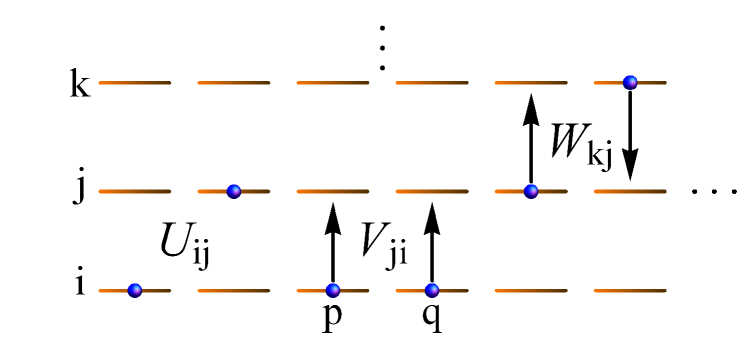
Figure 1: Schematic representation of the $U$, $V$ and $W$ couplings in the Hamiltonian (33).

As discussed in App. A, for full range couplings ($r_{pq}=\frac{1}{N-1}$ $\forall$ $p\neq q$) the present model comprises the fully connected $SU(n)$ fermionic nuclear models employed in Meshkov (1971); Nuñez et al. (1985); Rossignoli and Plastino (1987), which are an $n$-level generalization of the well-known two-level Lipkin model Lipkin et al. (1965); Tullio et al. (2019). Some $SU(n)$ spin models and magnets Manmana et al. (2011); Beverland et al. (2016); Romen and Läuchli (2020) also correspond to special cases of (33), with the $SU(n)$ invariant Heisenberg coupling Uimin (1970); Lai (1974); Sutherland (1975); Cazalilla and Rey (2014); Dufour et al. (2015); Nataf and Mila (2018) recovered for $V_{ij}=U_{ij}=0$ ($i\neq j$) and $W_{ij}=U_{ii}=J$. In its distinguishable formulation, (33) is an $n$ level extension of the anisotropic $XYZ$ spin $1/2$ Hamiltonian in an applied magnetic field Kurmann et al. (1982); Roscilde et al. (2004); Rossignoli et al. (2009); Canosa et al. (2020); Zvyagin (2021), recovered from (33) for $n=2$. Besides, for $n=2s+1$ Eq. (33) can be formulated as a system of spins $s$ with couplings depending on powers of the spin operators (see App. (A)).

Since particles are moved in pairs between levels, the Hamiltonian (33) has, for any value of the coupling strengths and range, the number parity symmetries

$$[H,P_{i}]= \;0,\;\;i=1,\ldots,n\,,$$ (34)

$$P_{i}= \exp[-i\pi N_{i}]\,,\;\;N_{i}=\sum_{p}c^{\dagger}_{pi}c_{pi}\,,$$ (35)

where $P_{i}$ is the parity of the total occupation $N_{i}$ of level $i$. Since $\prod_{i=1}^{n}P_{i}=e^{-i\pi N}$ is fixed, just $n-1$ parities are independent. The exact eigenstates of $H$ will then have definite parities when non-degenerate, and can be characterized by their $n-1$ values $\sigma_{i}=\pm 1$ for $i=2,\ldots,n$.

In the MF approximation, which in the uniform attractive case can be determined analytically (see App.  B) the GS of (33) will typically exhibit a series of transitions as the coupling strengths increase from $0$, from the unperturbed phase with all particles in the lowest $i=1$ level, to a final full parity-breaking phase where all $n$ levels are occupied, with intermediate steps where just $m<n$ levels are nonempty. These transitions become smoothed out in the actual entangled exact GS for finite $N$, which may instead exhibit number parity transitions (secs. III.2 and III.5). The parity-breaking MF GS becomes however exact at the factorization point, discussed below.

III.1 Uniform factorized GS

We now determine the conditions for which the Hamiltonian (33) possesses a uniform factorized GS

$$|\Psi\rangle=\prod_{p}a^{\dagger}_{p1}|0\rangle\,,\;\;a^{\dagger}_{p1}=\sum_{i}f_{i}c^{\dagger}_{pi}\,,$$ (36)

with $f_{i}$ $p$-independent and $\sum_{i}|f_{i}|^{2}=1$. We set $\epsilon_{i}^{p}=r_{p}\epsilon_{i}$ with $r_{p}=\sum_{q\neq p}r_{pq}$ according to (22), such that factorization is determined by the single Eq. (24).

It is then seen that for $k=i$, Eq. (19) leads here to

$$\sum_{j}[(2\epsilon_{i}-U_{ii})\delta_{ij}-V_{ij}]f_{j}^{2}=E_{2}f_{i}^{2}\,,$$ (37a)

for $$i=1,\ldots,n \bm{f}^{2} f_{i}^{2} M_{ij}=(2\epsilon_{i}-U_{ii})\delta_{ij}-V_{ij}$$, which is a standard eigenvalue equation for the vector of elements (i.e., for the “squared wave function”) and matrix :

$$M\bm{f}^{2}=E_{2}\bm{f}^{2}\,.$$ (37b)

It represents the $n\times n$ $ii$-$jj$ block in $\eqref{eqx2}$.

On the other hand, for $k=j\neq i$, Eq. (19) leads here to the $2\times 2$ $ij$-$ji$ block

$$\!\!\begin{pmatrix}\epsilon_{i}+\epsilon_{j}-U_{ij}&-W_{ij}\\ -W_{ij}&\epsilon_{i}+\epsilon_{j}-U_{ij}\end{pmatrix}\begin{pmatrix}f_{i}f_{j}\\ f_{j}f_{i}\end{pmatrix}=E_{2}\begin{pmatrix}f_{i}f_{j}\\ f_{j}f_{i}\end{pmatrix}\,.$$ (38)

Eq. (38) entails, for $f_{i}f_{j}\neq 0$, the constraint

$$U_{ij}+W_{ij}=\epsilon_{i}+\epsilon_{j}-E_{2}\,.$$ (39)

Hence, given an arbitrary single site spectrum $\epsilon_{i}$ and couplings $V_{ij}$, $U_{ii}$, the factorized eigenstate and pair energy $E_{2}$ are first determined from the eigenvalue equation (37b). The couplings $W_{ij}$ or $U_{ij}$ for which such state becomes an exact eigenstate are then obtained from (39). These conditions are independent of coupling range $r_{pq}$ and system size $N$, implying that this factorization will emerge for any $N\geq 2$ and range $r_{pq}$ if (39) is satisfied. The total energy is determined by $E_{2}$ through Eq. (25).

For GS factorization, the lowest eigenvalue $E_{2}$ of (37b) should be chosen. In this case, as the eigenvalues of the matrix in (38) are $\epsilon_{i}+\epsilon_{j}-U_{ij}\mp W_{ij}$, i.e. $E_{2}$ and $E_{2}+2W_{ij}$ when (39) is fulfilled, the uniform factorized state will be a GS of the full pair Hamiltonian (and hence of the full $H$) for any signs of the $V_{ij}$’s if

$$W_{ij}\geq 0\,\;\;\forall\,\,i\neq j\,,$$ (40)

i.e. $E_{2}\leq\epsilon_{i}+\epsilon_{j}-U_{ij}$ $\forall\,i\neq j$. Since the lowest eigenvalue of (37b) satisfies $E_{2}\leq{\rm Min}_{i}[2\epsilon_{i}-U_{ii}]\leq 2\epsilon_{i}-U_{ii}$ $\forall\,i$, a sufficient condition for the validity of (40) at fixed $U_{ij}$ is

$$U_{ij}\leq(U_{ii}+U_{jj})/2\,,$$ (41)

$\forall$ $i\neq j$. In particular, (40) will be always satisfied for the lowest eigenvalue $E_{2}$ if $U_{ij}=0$ $\forall$ $i,j$ and (39) is fulfilled. The factorized GS obtained from (37b) coincides, of course, with the MF GS for the couplings (39), lying within the full parity-breaking MF phase (see App. B).

For $n=2$, the factorization conditions (37b), (39) reduce to those for the $XYZ$ spin Hamiltonian (see App. A), leading to a factorizing field. And for $n=3$ it is still possible to satisfy (39) by adjusting just the one-site energies $\epsilon_{i}$, for given values of $U_{ij}$ and $W_{ij}$:

$$\epsilon_{i}={\textstyle\frac{1}{2}}(T_{ij}+T_{ik}-T_{jk}+E_{2})\,,$$ (42)

where $T=U+W$ and $i\neq j\neq k$. In this case a constant diagonal term $\Delta U_{ii}=U_{0}$ remains to be added in (37b) in order that $E_{2}$ matches the original value.

In the attractive case $V_{ij}\geq 0$ $\forall$ $i,j$, the eigenvector $\bm{f}^{2}$ of (37b) associated to the lowest eigenvalue $E_{2}$ will have all components $f_{i}^{2}$ of the same sign (in order to yield the lowest eigenvalue) and hence all $f_{i}$ can be chosen as real. Otherwise some of the $f_{i}^{2}$ can be negative, implying imaginary components $f_{i}$.

In systems which can be divided into even and odd sites such that any site $p$ is coupled ($r_{pq}\neq 0$) just to sites $q$ of opposite parity (like first neighbor couplings in a linear chain or cubic lattice), the uniform factorized GS can be used to generate, through local unitaries, alternating factorized GS’s for associated Hamiltonians. For instance, if $c^{\dagger}_{pi}\rightarrow-c^{{\dagger}}_{pi}$ for some level $i$ at odd sites $p$, then $V_{ij}\rightarrow-V_{ij}$, $W_{ij}\rightarrow-W_{ij}$ and $|\Psi\rangle$ is changed into an alternating product GS $|\Psi^{\prime}\rangle$ with $f_{i}^{p}\rightarrow(-1)^{p}f_{i}$.

III.2 Parity breaking and degeneracy at factorization

Eqs. (37b) just determine the squared coefficients $f_{i}^{2}$, leaving the sign of each $f_{i}$ free. This degeneracy of the uniform factorized eigenstate (36) reflects its breaking of all number parity symmetries $P_{i}$ if $f_{i}\neq 0$ $\forall\ i$: Its expansion in the standard “product” basis,

$$|\Psi\rangle=\sum_{i_{1},\ldots,i_{N}}f_{i_{1}}\ldots f_{i_{N}}c^{\dagger}_{1i_{1}}\ldots c^{\dagger}_{Ni_{n}}|0\rangle$$ (43)

clearly contains terms with all possible parities $P_{i}$. As

$$P_{i}c^{\dagger}_{pi}P_{i}^{\dagger}=-c^{\dagger}_{pi}\,,$$ (44)

$P_{i}|\Psi\rangle$ just changes the sign of $f_{i}$. Hence, if $|\Psi\rangle$ is an exact eigenstate, all $2^{n-1}$ parity transformed states

$$|\Psi_{i_{1}\ldots i_{m}}\rangle=P_{i_{1}}\ldots P_{i_{m}}|\Psi\rangle\,,$$ (45)

obtained by changing the signs of $f_{i_{1}}\ldots f_{i_{m}}$ in (43) with $m\leq n-1$, are also exact eigenstates with the same energy due to (34). These parity breaking product eigenstates can then only arise at a point where levels with different parities cross and become degenerate. Factorization then signals a fundamental parity level crossing taking place for any size $N$ and range $r_{pq}$ whenever Eq. (39) is fulfilled.

If $N\geq n-1$, we thus obtain from (45) $2^{n-1}$ nonorthogonal but linearly independent degenerate product eigenstates, implying a $D=2^{n-1}$ degeneracy at factorization, which indicates the number of distinct parity levels exactly crossing at this point.

On the other hand, for small systems with $N<n-1$, the number $D$ of linearly independent states obtained with such sign changes in the $f_{i}$, and hence the degeneracy at factorization is smaller. We obtain in general

$$D=\left\{\begin{array}[]{ccl}2^{n-1}&,&N\geq n-1\\ \sum_{k=0}^{N}\binom{n-1}{k}&,&N\leq n-1\end{array}\right.,$$ (46)

such that signs are to be changed in just $k\leq N$ levels. For a single pair ($N=2$), $D=\binom{n}{2}+1$.

We have so far assumed that the matrix $M$ in (37b) has a non-degenerate GS, with a full rank eigenvector $\bm{f}^{2}$. If $f_{i}=0$ for some $i$, then factorization (and the ensuing degeneracy) becomes equivalent to that for $n\rightarrow n-1$. And if the GS of $M$ is itself degenerate, the coefficients $f_{i}^{2}$ will no longer be unique (after normalization). The GS of $H$ will then exhibit additional degeneracy, since a continuous set of factorized GS’s becomes feasible. We will consider below a special extreme case.

III.3 The $W$-case: Number symmetry and exceptional degeneracy at factorization

We now consider the special case where $V_{ij}=0$ $\forall$ $i\neq j$ in (33). For $n=2$ it corresponds to the $XXZ$ model (see App. A) which conserves the total $S_{z}$ and hence has eigenstates with definite magnetization. Accordingly, for $V_{ij}=0$ Eq.  (33) exhibits an additional symmetry: not only parity but also the total occupation of each level is conserved:

$$[H,N_{i}]=0\,,\;\;\;i=1,\ldots,n\,,$$ (47)

since the $U$ and $W$ couplings preserve all $N_{i}$’s. The exact eigenstates can then be characterized by the occupations $N_{i}$ of each level, existing $\frac{N!}{N_{1}!\ldots N_{n}!}$ orthogonal states with the same set of occupations $(N_{1},\ldots,.N_{n})$.

This higher symmetry entails, first, a trivial factorization: the $n$ states with all particles in just one level,

$$|\Psi_{i}\rangle=\prod_{p}c^{\dagger}_{pi}|0\rangle\,,\;\;\;i=1,\ldots,n\,,$$ (48)

are clearly exact eigenstates: $H|\Psi_{i}\rangle=E_{i}|\Psi_{i}\rangle$ with $E_{i}=(\epsilon_{i}-\frac{1}{2}U_{ii})\sum_{p}r_{p}$. For $n=2$ they become the fully aligned spin states with maximum magnetization $|M|$.

But in addition, non-trivial symmetry-breaking uniform factorized eigenstates of the form (36) may also arise: Eqs. (37b)–(39) remain valid, but Eq.  (37b) becomes trivial, implying, for a full rank solution with $f_{i}\neq 0$ $\forall i$,

$$U_{ii} = 2\epsilon_{i}-E_{2}\,,\;\;i=1,\ldots,n\,,$$ (49)

$$W_{ij}+U_{ij} = \epsilon_{i}+\epsilon_{j}-E_{2}={\textstyle\frac{U_{ii}+U_{jj}}{2}}\,.$$ (50)

Thus, $f_{i}$ remains here completely arbitrary: For vanishing $V_{ij}$ any uniform factorized state (36) is an exact eigenstate with the same energy (25) when (49)–(50) are fulfilled, as the matrix $M$ becomes proportional to the identity. And if $W_{ij}\geq 0$ $\forall$ $i\neq j$, i.e. if Eq. (41) holds $\forall$ $i\neq j$, they will be GS’s by the same previous arguments. The ensuing GS energy (25) is then independent of the number $n$ of levels for a given fixed value of $E_{2}$.

Such continuous set of factorized exact GS’s reflects their breaking of all number symmetries (47) when $0<f_{i}<1$ $\forall\ i$, as they lead to non-zero fluctuations $\langle N_{i}^{2}\rangle-\langle N_{i}\rangle^{2}=Nf_{i}(1-f_{i})>0$. Moreover, since they contain terms with all possible values $0\leq N_{i}\leq N$ when $f_{i}\neq 0$ $\forall$ $i$, all number projected states with definite values $N_{i}=n_{i}$ $\forall\ i$ derived from such product state $|\Psi\rangle$,

$$|\Psi_{n_{1}\ldots n_{n}}\rangle\propto P_{n_{1}}\ldots P_{n_{n}}|\Psi\rangle\,,$$ (51)

satisfying $N_{i}|\Psi_{n_{1}\ldots n_{n}}\rangle=n_{i}|\Psi_{n_{1}\ldots n_{n}}\rangle$ with $\sum_{i=1}^{n}n_{i}=N$, will also be exact eigenstates with the same energy due to (47). Here $P_{n_{i}}=\frac{1}{2\pi}\int_{0}^{2\pi}e^{-\imath\phi(N_{i}-n_{i})}d\phi$ are number projectors ($[P_{n_{i}},H]=0$ $\forall$ $i$).

Remarkably, when normalized these projected states become independent of the arbitrary coefficients $f_{i}$ determining the product state $|\Psi\rangle$, since each term in their expansion (43) will have exactly $n_{i}$ particles in level $i$ and hence all coefficients become identical: $f_{i1}\ldots f_{i_{N}}=\prod_{i=1}^{n}(f_{i})^{n_{i}}=C_{n_{1}\ldots n_{n}}$. Therefore, the states (51) become

$$|\Psi_{n_{1}\ldots n_{n}}\rangle=|n_{1}\ldots n_{n}\rangle\,,$$ (52)

where $|n_{1}\ldots n_{n}\rangle$ is the fully symmetric state having $N_{i}=n_{i}$ particles in each level $i$. The total degeneracy at factorization is then given by the number of distinct projected states (52), which is just the number of ways of distributing $N$ undistinguishable particles on $n$ levels:

$$D=\binom{N+n-1}{n-1}\,,$$ (53)

with $D\approx\frac{N^{n-1}}{(n-1)!}$ for $N\gg n$. Then factorization arises at an exceptional critical point where the $D$ lowest levels with distinct values of the $N_{i}$’s cross and become degenerate. The ensuing degeneracy grows with system size, in contrast with previous $N$-independent parity degeneracy.

Since any uniform factorized state is an exact GS at the factorizing point, the GS subspace is here clearly invariant under arbitrary $U(n)$ unitary transformations

$$U=\exp[-i\sum_{i,j}T_{ij}\sum_{p}c^{\dagger}_{pi}c_{pj}]\,,$$ (54)

where $T$ is an arbitrary hermitian matrix, as $U$ transforms any product state (36) into another uniform product state and these states span the GS subspace:

$$|\Psi\rangle\rightarrow U|\Psi\rangle\;\Longrightarrow\;\bm{f}\rightarrow\exp[-iT]\bm{f}\,.$$ (55)

It corresponds to $U=e^{-iT}\!\otimes\ldots\otimes e^{-iT}$ in the distinguishable formulation.

The question which now arises is whether the full $H$ also becomes $SU(n)$ invariant when the factorizing conditions (49)–(50) are fulfilled. For $n=2$ this is indeed the case: as shown in App. A, they lead to a Heisenberg Hamiltonian $H\propto-\sum_{p<q}r_{pq}\bm{s}_{p}\cdot\bm{s}_{q}$ plus constant terms, where $\bm{s}_{p}$ is the (dimensionless) spin operator at site $p$. Such $H$ is obviously invariant under arbitrary global rotations $e^{-i\phi\bm{k}\cdot\sum_{p}\bm{s}_{p}}$, with $\bm{k}$ an arbitrary unit vector, and admits any aligned product state $|\bm{k},\ldots,\bm{k}\rangle$, with $\langle\bm{k}|\bm{s}_{p}|\bm{k}\rangle=\frac{1}{2}\bm{k}$, as exact GS for arbitrary $\bm{k}$.

However, for $n\geq 3$ only the GS subspace remains invariant in general, i.e., $[H,U]\neq 0$, with $[H,U]$ having just $D$ zero eigenvalues, corresponding to the GS subspace. Therefore, for $n\geq 3$ the general $SU(n)$ Heisenberg Hamiltonian Uimin (1970); Lai (1974); Sutherland (1975)

$$H=-J\sum_{p<q}r_{pq}\sum_{i,j}c^{\dagger}_{pi}c^{\dagger}_{qj}c_{qi}c_{pj}$$ (56)

is just a particular case of present factorizing Hamiltonian, corresponding to $\epsilon_{i}=0$ $\forall$ $i$ and hence $U_{ii}=J=-E_{2}=W_{ij}$ $\forall$ $i\neq j$, according to Eqs.  (49)–(50).

III.4 Definite parity eigenstates and entanglement at the border of factorization

We now examine the GS in the immediate vicinity of factorization. We consider first the $V\neq 0$ case. Since away from factorization the exact GS is normally non-degenerate for finite $N$, it will have definite parities $P_{i}$. The same holds for the other levels which meet at the factorization point. Therefore, their side-limits at factorization will be given by the parity projected states

$$|\Psi_{\sigma_{2}\ldots\sigma_{n}}\rangle\propto(\mathbbm{1}+\sigma_{2}P_{2})\ldots(\mathbbm{1}+\sigma_{n}P_{n})|\Psi\rangle\,,$$ (57)

where $\sigma_{i}=\pm 1$, satisfying $P_{i}|\Psi_{\sigma_{2}\ldots\sigma_{n}}\rangle=\sigma_{i}|\Psi_{\sigma_{2}\ldots\sigma_{n}}\rangle$ $\forall i$. This projection just selects from the expansion (43) those terms with the specified level parities. The GS will then exhibit a parity transition as the factorization point is crossed Rossignoli et al. (2008, 2009); Canosa et al. (2020) (when some Hamiltonian parameter is varied), having distinct parities $\sigma_{i}$ at each side.

These projected states are entangled, i.e., they are no longer product states. They exhibit critical entanglement properties since the product state $|\Psi\rangle$ from which they are derived is uniform and has lost all information about the range $r_{pq}$ of the coupling and the distance between sites. Accordingly, the exact side-limits at factorization of GS entanglement entropies will be range-independent. Moreover, pairwise entanglement will be independent of the separation $|p-q|$ between sites, although it will remain small in compliance with monogamy Coffman et al. (2000); Osborne and Verstraete (2006).

These properties can be seen, for instance, in the reduced state of site $p$, $\rho_{p}={\rm Tr}_{p^{\prime}\neq p}|\Psi_{0}\rangle\langle\Psi_{0}|$, of elements

$$(\rho_{p})_{ij}=\langle c^{\dagger}_{pj}c_{pi}\rangle\,,$$ (58)

and eigenvalues $\lambda_{pi}$. Its entropy

$$S_{p}=-{\rm Tr}\,\rho_{p}\log_{2}\rho_{p}=-\sum_{i=1}^{n}\lambda_{pi}\log_{2}\lambda_{pi}$$ (59)

is a measure of the (mode) entanglement between this site and remaining sites. In the fermion case it is also a measure of fermionic entanglement Gigena and Rossignoli (2015); Tullio et al. (2019), in the sense of indicating the deviation of the state from an independent fermion state [Slater Determinant (SD)], since it is the $p$-block of the one-body density matrix $\rho^{(1)}$:

$$\rho^{(1)}_{pi,qj}=\langle c^{\dagger}_{qj}c_{pi}\rangle=\delta_{pq}\langle c^{\dagger}_{pj}c_{pi}\rangle\,,$$ (60)

whose blocked structure is due to the fixed fermion number $N_{p}$ at each site. Its entropy $S(\rho^{(1)})=\sum_{p}S_{p}$ is a quantity which vanishes iff $|\Psi_{0}\rangle$ is a SD, i.e.  $(\rho^{(1)})^{2}=\rho^{(1)}$ Gigena and Rossignoli (2015); Di Tullio et al. (2018), and is just $NS_{p}$ in the uniform case. In the factorized state $|\Psi\rangle$, $\langle c^{\dagger}_{pj}c_{pi}\rangle=f^{p*}_{i}f^{p}_{j}$, implying obviously $\rho_{p}^{2}=\rho_{p}$, i.e., $\lambda_{pi}=\delta_{i1}$, as directly seen in the MF basis ($\langle a^{\dagger}_{pj}a_{pi}\rangle=\delta_{ij}\delta_{i1}$), and hence $S_{p}=0$.

In contrast, in states $|\Psi_{0}\rangle$ with definite parity all off-diagonal elements in the standard basis are cancelled by parity conservation ($[\rho_{p},e^{i\pi c^{\dagger}_{pi}c_{pi}}]=0$ $\forall$ $i$), implying

$$\langle c^{\dagger}_{pj}c_{pi}\rangle=\delta_{ij}\langle c^{\dagger}_{pi}c_{pi}\rangle\,.$$ (61)

Hence the eigenvalues of $\rho_{p}$ are just the average occupations $\lambda_{pi}=\langle c^{\dagger}_{pi}c_{pi}\rangle$ and $S_{p}>0$ whenever $\langle c^{\dagger}_{pi}c_{pi}\rangle\in(0,1)$.

In the projected states (57), these occupations depend on the parities $\sigma_{2},\ldots,\sigma_{n}$. For instance, for $n=3$ in the uniform case, we obtain, for $i=1,\ldots,3$,

$$\langle\Psi_{\sigma_{2}\sigma_{3}}|c^{\dagger}_{pi}c_{pi}|\Psi_{\sigma_{2}\sigma_{3}}\rangle\ =|f_{i}|^{2}{\textstyle\frac{1+\sum_{j}(-1)^{\delta_{ij}}\sigma_{j}(1-2|f_{j}|^{2})^{N-1}}{1+\sum_{j}\sigma_{j}(1-2|f_{j}|^{2})^{N}}}$$ (62)

where $\sigma_{1}\sigma_{2}\sigma_{3}=(-1)^{N}$. Hence, for large $N$ $\lambda_{pi}\approx|f_{i}|^{2}$ plus corrections of order $(1-2|f_{j}|^{2})^{N-1}$, which depend on the parities $\sigma_{j}$.

For finite $N$ these corrections are, nonetheless, appreciable and their parity dependence originates the splitting of the degeneracy in the immediate vicinity of factorization (App. C). Moreover, the occupations (62) determine the exact side-limits of the single-site entanglement entropy (59) at factorization, which will then remain finite at this point and exhibit a discontinuity due to the change in the GS parities $\sigma_{i}$. For large $N$ this discontinuity becomes small, as $\lambda_{pi}\approx|f_{i}|^{2}$ approaches the MF value at both sides, but the side-limits of $S_{p}$ remain finite.

On the other hand, the entanglement between two sites $p\neq q$ is determined by their reduced pair state $\rho_{pq}={\rm Tr}_{p^{\prime}\neq p,q}|\Psi_{0}\rangle\langle\Psi_{0}|$, also a mixed state. For general $n$ it can be measured through the negativity Vidal and Werner (2002); Zyczkowski et al. (1998); Plenio (2005)

$${\cal N}_{pq}=\frac{1}{2}({\rm Tr}|\rho^{T_{p}}_{pq}|-1)\,,$$ (63)

where $\rho^{T_{p}}_{pq}$ is the partial transpose of $\rho_{pq}$. Eq. (63) is just minus the sum of the negative eigenvalues of $\rho^{T_{p}}_{pq}$, with ${\cal N}_{pq}>0$ ensuring entanglement of $\rho_{pq}$ according to Peres criterion Peres (1996). The side-limits at factorization of the exact GS negativities will be determined by the projected states (57), and will be non-zero for finite $N$, and hence independent of the separation between sites and the coupling range for a uniform $|\Psi\rangle$, undergoing there a discontinuity due to the transition in the GS parities.

While visible in small systems (see sec. III.5), the common value of ${\cal N}_{pq}$ at factorization decreases as $N$ increases, in agreement with monogamy: The projected states (57) involve a sum over $2^{n-1}$ product states $\sigma_{i_{1}}P_{i_{1}}\ldots\sigma_{i_{m}}P_{i_{m}}|\Psi\rangle$ having the signs of $f_{i}$ changed at levels $i_{1},\ldots,i_{m}$, which for sufficiently large $N$ become approximately orthogonal (e.g. for $n=3$ their overlaps are proportional to terms $(1-2|f_{j}|^{2})^{N}$, as seen in (62), which decrease rapidly with $N$ if $|f_{j}|\neq 0$ or $1$). Neglecting these overlaps, the two-site reduced states $\rho_{pq}$ derived from (57) become essentially a convex mixture of $2^{n-1}$ product states $\rho_{p}\otimes\rho_{q}$, and are then separable Peres (1996), implying ${\cal N}_{pq}\approx 0$ $\forall$ $p,q$. Thus, for large systems pairwise entanglement vanishes at factorization, though it will still show long range in its vicinity Amico et al. (2006); Rossignoli et al. (2009); Canosa et al. (2020).

We remark, however, that the exact GS side-limits at factorization of other entanglement measures do remain finite for large $N$, as was seen for the single site entropy (59). In fact, previous argument entails that the reduced state $\rho_{M}\equiv\rho_{p_{1}\ldots p_{M}}$ of $M<N$ sites derived from (57) will be mixed with rank $2^{n-1}$ (for $M\geq n-1$), such that its entropy, measuring their entanglement with the rest of the system, will also have non-zero side-limits for any $N$. They will be bounded, however, by this rank:

$$S(\rho_{M})=-{\rm Tr}\,\rho_{M}\log_{2}\rho_{M}\leq n-1\,,$$ (64)

at the border of factorization. This bound at this point is then another signature of factorization in these systems.

Similar considerations hold for the $V=0$ case. The level number projected states (51)–(52) represent the exact side-limits at factorization of the $D$ crossing states. Except for the states (48) with just one level occupied, all remaining states are entangled and lead again to critical entanglement properties (independence of coupling range and separation) due to their fully symmetric nature. In particular, they lead again to single site reduced states $\rho_{p}$ diagonal in the standard basis,

$$\langle n_{1}\ldots n_{n}|c^{\dagger}_{pi}c_{p_{j}}|n_{1}\ldots n_{n}\rangle=\delta_{ij}n_{i}/N\,,$$ (65)

implying $\lambda_{pi}=n_{i}/N$ and hence a single-site entropy $S(\rho_{p})>0$ if $1\leq n_{i}\leq N-1$ at least for some $i$.

III.5 Factorization signatures in small systems

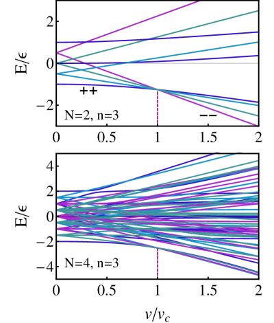
Figure 2: The exact spectrum of Hamiltonian (33) for a single pair ($N=2$, top) and for $N=4$ sites (bottom), with first neighbor couplings and $n=3$ levels at each site, as a function of the scaled coupling strength $v/v_{c}$ (see text). In both cases factorization takes place at the same value $v=v_{c}$, where Eqs. (37b)-(39) are fulfilled and the four levels with distinct parities forming the GS band cross.

We discuss here typical illustrative results in small $n$-level systems. We examine first the case with both $V$ and $W$ couplings of sections III.1-III.2. We consider a uniform single site spectrum $\epsilon_{i}=\frac{\epsilon}{2}(i-\frac{n+1}{2})$ for $i=1,\ldots,n$, and couplings $U_{ij}=0$, $V_{ij}=v$ and $W_{ij}=(v/v_{c})(\epsilon_{i}+\epsilon_{j}-E_{2c})$, chosen such that GS factorization is reached at $v=v_{c}$, according to Eq. (39) ($E_{2c}$ is the pair energy obtained from (37b) at $v=v_{c}$). For $n=2$ these parameters lead to an anisotropic $XY$ Heisenberg coupling in a uniform field (Eq. (68) with $J_{z}=0$), while for general $n$ it is an extension of the $n$-level model used in Nuñez et al. (1985); Rossignoli and Plastino (1987). Figs. 2–5 show results for the $n=3$-level case with $v_{c}=\frac{2}{5}\epsilon$ (for which $E_{2c}\approx-1.26\epsilon$).

We first depict in Fig. 2 the spectrum of $H$ for a single pair ($N=2$, $r_{12}=1$) and for a cyclic four-particle chain with first-neighbor couplings ($N=4$, $r_{pq}=\frac{1}{2}\delta_{q,p\pm 1}$), as a function of $v/v_{c}$. In both cases there is a GS band of $2^{n-1}=4$ states which cross exactly at the factorization point $v=v_{c}$, where a GS number parity transition takes place: The GS changes from the $(\sigma_{1},\sigma_{2})=(+,+)$ state for $v<v_{c}$, to the $(\sigma_{1},\sigma_{2})=(-,-)$ state for $v>v_{c}$. These states form the border of the GS band, the remaining crossing levels $(\sigma_{1},\sigma_{2})=(\pm,\mp)$ lying in between.

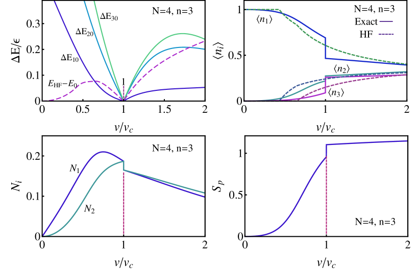
Figure 3: Results for the $N=4$ chain of Fig. 2. Top left: The first three exact excitation energies $\Delta E_{i0}=E_{i}-E_{0}$ and the difference $E_{\rm HF}-E_{0}$ with the Hartree-Fock (HF) GS energy. All vanish at the factorization point $v=v_{c}$ (1). Top right: Exact (solid lines) and HF (dotted lines) values of the GS average occupations $\langle n_{i}\rangle=\langle c^{\dagger}_{pi}c_{pi}\rangle$ of the three levels. The exact values represent the eigenvalues of the single site reduced density matrix and exhibit a discontinuity at $v=v_{c}$. Bottom: The exact one-site entanglement entropy (59) (right), which shows a stepwise increase at factorization, and the exact negativities between first (${\cal N}_{1}={\cal N}_{p,p+1}$) and second (${\cal N}_{2}$) neighbors (left), measuring pairwise entanglement. Both reach the same side-limits at factorization, exhibiting there a stepwise decrease.

Further results for a ring of $N=4$ particles are shown in Fig. 3. It is verified that the first three exact excitation energies, together with the difference with the mean field (HF, see App. B) GS energy, exactly vanish just at $v=v_{c}$ (top left), confirming factorization. The exact average occupations $\langle n_{i}\rangle$ of each level are shown in the top right panel (solid lines). As $v$ increases the two upper levels start to be populated, with all exact occupations undergoing a step-like discontinuity at the factorizing point, reflecting the associated GS parity transition. The side-limits at this point coincide with those determined by the projected states (57) through Eq. (62). Present factorization can then be detected and verified through the magnitude of these occupation jumps.

HF results reproduce qualitatively the general trend but miss the jump at factorization: Though exact at this point, the HF GS corresponds to a superposition of the crossing definite parity exact eigenstates. It exhibits instead transitions at $v/v_{c}\approx 0.44$ and $0.65$ ($\forall\,N$), where the second and third level respectively start to be populated in the approach (see App. B) and parity symmetry becomes broken. Thus, factorization lies within the full parity-breaking HF phase (and not at a HF transition).

Entanglement properties are depicted in the lower panels. The exact single site entanglement entropy (59) (bottom right) increases monotonously as $v/v_{c}$ increases, and displays a stepwise increase precisely at the factorizing point, due to the transition in the average level occupations. The negativities ${\cal N}_{1}$ and ${\cal N}_{2}$ (bottom left), measuring the pairwise entanglement between first and second neighbors, exhibit instead a stepwise decrease at factorization, indicating multipartite entanglement effects of the parity projected states. They are also verified to approach the same side-limits at factorization, confirming the independence from separation in its immediate vicinity, as predicted by the projected states (57).

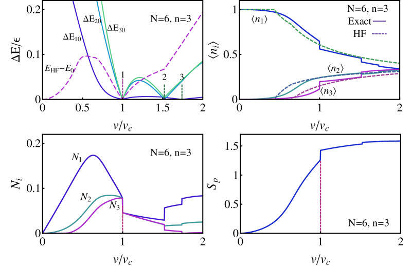
Figure 4: Results for an $N=6$ chain with $n=3$ levels at each site. Details are similar to those of Fig. 3. Top left: The first three excitation energies $\Delta E_{i0}$ together with $E_{\rm HF}-E_{0}$. Points $2,3$ indicate other GS parity transitions. Top right: Exact and HF average occupations $\langle n_{i}\rangle$. Bottom: The one-site entanglement entropy (59) (right) and the exact negativities between first, second and third (${\cal N}_{3}$) neighbors (left). All ${\cal N}_{i}$ reach the same side-limits just at factorization ($v=v_{c}$).

In Fig. 4 we show the same quantities for a ring of $N=6$ particles with the same parameters, to view the trend for larger systems. Their behavior remains similar, with factorization located at the same point, where the four lowest levels with distinct parities cross (top left). However, the GS now exhibits in the range considered two further parity transitions, at $v_{c2}\approx 1.52v_{c}$ and $v_{c3}\approx 1.74v_{c}$, not related to factorization, where just two levels cross and the GS parity changes from $(\sigma_{2},\sigma_{3})=(+,+)$ for $v<v_{c}$ to $(-,-)$ for $v_{c}<v<v_{c2}$, $(+,-)$ for $v_{c2}<v<v_{c3}$ and back to $(+,+)$ for $v>v_{c3}$.

These transitions lead to further steps in the single site occupation numbers and entropy (right panels), though the larger step occurs again at the factorizing transition. All three pair negativies ${\cal N}_{i}$ are verified to reach the same side-limits at the factorizing point, a characteristic signature of uniform factorization, exhibiting there a stepwise decrease. These patterns are not repeated at the other GS parity transitions, where ${\cal N}_{1}$ increases but ${\cal N}_{3}$ decreases, vanishing for $v>v_{c3}$. Full range pairwise entanglement is thus centered at the factorizing point, where it becomes independent of separation. However, the side-limits of ${\cal N}$ at factorization are smaller than for $N=4$, in agreement with monogamy and previous considerations.

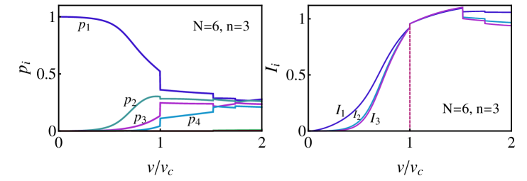
Figure 5: The exact eigenvalues of the two-site reduced density matrix for first neighbors (left) and the mutual information $I(\rho_{pq})$ for first ($I_{1}$), second ($I_{2}$) and third ($I_{3}$) neighbors (right), in the chain of Fig. 4. All $I_{i}$ exactly merge at the side-limits of the factorizing point $v=v_{c}$.

In Fig. 5 we show the eigenvalues $p_{i}$ (entanglement spectrum) of the two-site density matrix $\rho_{pq}$ (left panel), which determine the entanglement of the pair with the rest of the chain (just $4$ of them are nonnegligible). They also exhibit steps at the parity transitions, with the larger step again at the factorizing point. The ensuing mutual information

$$I_{pq}=S(\rho_{p})+S(\rho_{q})-S(\rho_{pq})$$ (66)

where $S(\rho_{p})=S_{p}$ is the single site entropy, is shown on the right panel for the first three neighbors. It is a measure of the total correlation between sites. It is seen that all three values merge at the side-limits of the factorizing point, confirming again that in its vicinity correlations become independent of separation. Since it does not satisfy monogamy, its behavior is, however, different from that of the negativity, steadily increasing up to $v_{c2}$ and exhibiting at factorization a stepwise increase.

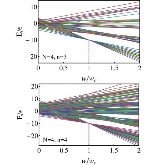
Figure 6: The exact spectrum of Hamiltonian (33) for $V_{ij}=0$ and first neighbor $W$ and $U$ couplings (see text), for $N=4$ sites and $n=3$ (top) and $4$ (bottom) levels at each site, as a function of the scaled coupling strength $w/w_{c}$. Factorization arises at an exceptionally degenerate point $w=w_{c}$ where $15$ ($35$) levels cross for $n=3$ ($4$), in agreement with Eq. (53). At this point any uniform factorized state is an exact GS.

Finally, Figs. 6 and 7 show the spectrum of $H$ in the special $W$ case ($V_{ij}=0$) of sec. III.3, for $N=4$ particles and cyclic first neighbor couplings. In Fig. 6 we consider $n=3$ (top) and $4$ (bottom) levels at each site, with uniform spectrum $\epsilon_{1}=-\epsilon$, $\epsilon_{2}=0$, $\epsilon_{3}=0.8\epsilon$ (and $\epsilon_{4}=2.2\epsilon$ for $n=4$), unequally spaced in order to avoid extra degeneracy away from factorization. We have set $U_{ij}=\delta_{ij}\frac{w}{w_{c}}(2\epsilon_{i}-E_{2})$ and $W_{ij}=\frac{w}{w_{c}}(\epsilon_{i}+\epsilon_{j}-E_{2})$, with $w_{c}=\epsilon$ and $E_{2}=-5\epsilon$, such that factorization takes place at $w=w_{c}$ according to Eqs. (49)–(50), with GS energy $\frac{N}{2}E_{2}=-\frac{5}{2}N\epsilon$, independent of $n$.

It is verified that all $\binom{N+n-1}{N}$ levels ($15$ for $n=3$ and 35 for $n=4$) forming the “GS band” cross at the factorization point $w=w_{c}$, where any uniform product state is confirmed to be an exact GS. The side-limits at $w=w_{c}$ of the crossing states are the symmetric states (52) with definite occupations in all $n$ levels, whose energies become all identical at this point, with the GS changing at $w_{c}$ from $|\Psi_{1}\rangle$ (Eq. (48), all particles in the first level) to $|\Psi_{n}\rangle$ (all particles in the last level). No other multilevel crossing in higher excited states occurs at this point.

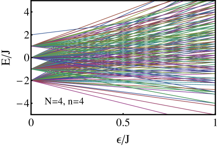
Figure 7: The spectrum of Hamiltonian (33) for $V_{ij}=0$ and $U_{ii}=W_{ij}=J$ $\forall$ $i,j$, as a function of the single particle spacing $\epsilon/J$, for $N=n=4$ (see text). For $\epsilon\rightarrow 0$ the $SU(n)$ invariant Hamiltonian (56) is approached. In this limit any uniform factorized state is again an exact GS, with the GS degeneracy ($D=35$) given by the same Eq. (53).

To complete the description, Fig. 7 depicts the spectrum for fixed couplings $W_{ij}=U_{ii}=J>0$ $\forall\,i,j$ and previous single site energies, as a function of the spacing $\epsilon$ for $n=4$ levels. At fixed $J$ factorization is then reached for $\epsilon\rightarrow 0$, where $H$ becomes the $SU(n)$ invariant Hamiltonian (56) and Eqs. (49)–(50) are fulfilled, with $E_{2}=-J$ and GS energy $-NJ/2$ $\forall$ $n\geq 2$. Again, all $35$ levels of the initial GS band merge in this limit, where any uniform product state becomes an exact GS.

However, in contrast with Fig. 6, it is seen that the remaining higher energy levels also coalesce for $\epsilon\rightarrow 0$ into four levels, three of them highly degenerate (the highest level remains nondegenerate), due the high symmetry of $H$ for $\epsilon=0$. Nevertheless, these higher energy eigenspaces contain no fully factorized states. As can be seen from (49)–(50), even if nonuniform product states were considered, no further fully separable eigenstate is feasible for $\epsilon=0$, apart from those of the GS subspace.

For $N=4$ and $n\geq 4$, the spectrum of Hamiltonian (56) with first neighbor couplings has just five distinct energies with uniform spacing: $E_{i}=-J(3-i)$ for $i=1,\ldots,5$. For $n=4$ the level degeneracies are $(35,110,60,50,1)$, the highest level corresponding to the fully antisymmetric eigenstate. We remark, however, that while the same factorized GS’s hold also in the presence of long range or nonuniform couplings, i.e. arbitrary $r_{pq}>0$, with the same degeneracy (53) (and also the same energy if $r_{p}=\sum_{q\neq p}r_{pq}=1$ $\forall\,p$), the intermediate levels and degeneracies do depend on the coupling range and $r_{pq}$, and are hence not “universal”. Only the fully antisymmetric eigenstates, feasible for $n\geq N$, remain also unaltered, with an energy which is just the opposite of that of the fully symmetric factorized eigenstates.

IV Conclusions

We have analyzed the problem of GS factorization beyond the standard interacting spin system scenario. We have first derived general necessary and sufficient factorization conditions for Hamiltonians with two-site couplings, showing that they can be recast as pair eigenvalue equations. These conditions were then applied to interacting $N$-particle systems, where each constituent has access to $n$ local levels. For the $UVW$ class of Hamiltonians (33) they can be worked out explicitly, leading in the uniform case to the eigenvalue equation (37b) for the squared local wave function and the constraint (39) on the coupling strengths, valid for any number $n$ of levels. They are independent of size $N$ and coupling range, and generalize those for $XYZ$ spin systems, recovered for $n=2$. The ensuing product state is shown to be a GS when conditions (40) are fulfilled, which are directly satisfied for vanishing $U_{ij}$.

The full rank factorized GS breaks all level number parities, preserved by the Hamiltonian, therefore having a $2^{n-1}$ degeneracy (for $N\geq n-1$). Factorization then arises at a special point where all $2^{n-1}$ definite parity levels of the GS band cross and become degenerate, signaling a fundamental GS level parity transition emerging for any size $N$ and range.

We have also examined the special $V=0$ case, where the Hamiltonian preserves the total occupation of each level. Here the factorization conditions allowed us to identify an exceptional critical point, again emerging for any size and range, where all levels with definite occupations $N_{i}$ forming the GS band coalesce and become degenerate. This leads to a GS degeneracy which increases with system size ($D\propto N^{n-1}$). At this point all uniform product states, including those breaking all occupation number symmetries, are exact degenerate GSs, implying a full $SU(n)$ invariant GS subspace, in a Hamiltonian which for $n\geq 3$ is not necessarily $SU(n)$ invariant.

Finally, we have analyzed the entanglement properties in the immediate vicinity of factorization. For small systems, pairwise entanglement (as detected by the negativity) reaches there full range and becomes independent of separation, thus constituting an entanglement critical point. Moreover, in such systems the parity transition occurring at the factorizing point entails finite discontinuities in most quantities (single site entanglement, negativity, level occupations, mutual information, etc.), whose magnitude can be analytically determined through projection of the factorized GS. On the other hand, for large systems pairwise entanglement will become vanishingly small at factorization for any pair, but long range entanglement in its vicinity as well other effects (like bounded values of block entropies, Eq. (64)) will remain visible.

In summary, in addition of providing nontrivial analytic exact GSs in strongly coupled systems which are not exactly solvable (which could be used as benchmarks for approximate numerical techniques), symmetry-breaking factorization enables one to identify critical points in small samples with exceptional GS degeneracy and entanglement properties. Amidst increasing quantum control capabilities, present results open the way to explore factorization in $SU(n)$ many-body physics and complex systems beyond the usual $SU(2)$ spin scenario.

Appendix A Special cases of Hamiltonian (33)

We consider here particular cases of Hamiltonian (33). Fully connected fermionic $U(n)$ nuclear models as those used in Meshkov (1971); Nuñez et al. (1985), correspond to $r_{pq}=\frac{1}{N-1}$ $\forall$ $p\neq q$. In this case, for $U_{ij}=0$ and $\epsilon_{i}^{p}=\epsilon_{i}$ we can rewrite (33) as

$$H=\sum_{i=1}^{n}\epsilon_{i}G_{ii}-{\textstyle\frac{1}{2(N-1)}}\sum_{i\neq j}V_{ij}G_{ij}^{2}+W_{ij}(G_{ij}G_{ji}-G_{ii})\,,$$ (67)

where $G_{ij}=\sum_{p=1}^{\Omega}c^{\dagger}_{pi}c_{pj}$ are collective operators satisfying the same $U(n)$ algebra as the operators $g_{ij}=c^{\dagger}_{pi}c_{pj}$:

$$[G_{ij},G_{kl}]=\delta_{jk}G_{il}-\delta_{il}G_{kj}\,,$$

for both fermions and bosons. Eq. (67) is a simplified schematic model for describing collective excitations. For $n=2$ and $\epsilon_{i}=(-1)^{i}\epsilon/2$ it becomes the Lipkin Hamiltonian Lipkin et al. (1965); Tullio et al. (2019)

$$H=\epsilon S_{z}-{\textstyle\frac{1}{2(N-1)}}[V(S_{+}^{2}+S_{-}^{2})+W(S_{+}S_{-}+S_{-}S_{+}-N)]$$

where $S_{z}=\frac{1}{2}(G_{22}-G_{11})$, $S_{+}=G_{21}=S_{-}^{\dagger}$ are collective spin operators satisfying the $SU(2)$ algebra ($[S_{z},S_{\pm}]=\pm S_{\pm}$, $[S_{-},S_{+}]=2S_{z}$) and $V=V_{12}$, $W=W_{12}$. These models have been used to test several many-body techniques Lipkin et al. (1965); Nuñez et al. (1985); Rossignoli and Plastino (1987); Tullio et al. (2019); Ring and Schuck (2004), as the exact eigenstates can be obtained by diagonalizing $H$ in the irreducible representations of $U(n)$. For $n=2$ level number parity conservation reduces to the $S_{z}$-parity symmetry $[H,P_{z}]=0$, where $P_{z}=e^{-i\pi S_{z}}=P_{2}e^{-i\pi N}$.

On the other hand, in the distinguishable formulation, the Hamiltonian (33) corresponds, for $g_{p}^{ij}=|i_{p}\rangle\langle j_{p}|$, to

$$H=\sum_{i,p}\epsilon_{i}^{p}g_{p}^{ii}-\!\!\sum_{p<q,i,j}\!\!r_{pq}(U_{ij}g_{p}^{ii}g_{q}^{jj}+V_{ij}g_{p}^{ij}g_{q}^{ij}+W_{ij}g_{p}^{ij}g_{q}^{ji})\,.$$

For $n=2$, $\epsilon^{p}_{i}=(-1)^{i}b^{p}/2$, $V_{12}=(J_{x}-J_{y})/2$, $W_{12}=(J_{x}+J_{y})/2$ and $U_{11}=U_{22}=-U_{12}=J_{z}/2$, with $p=1,\ldots,N$, it becomes the Hamiltonian of $N$ spins $1/2$ interacting through anisotropic $XYZ$ couplings Roscilde et al. (2004); Baxter (1971); Rossignoli et al. (2009); Zvyagin (2021) of general range in a nonuniform field $b^{p}$:

$$H=\sum_{p}b^{p}s_{pz}-\sum_{p\neq q}r_{pq}\!\!\sum_{\mu=x,y,z}J_{\mu}s_{p\mu}s_{q\mu}\,,$$ (68)

where $s_{pz}=\frac{g_{p}^{22}-g_{p}^{11}}{2}$, $s_{px}=\frac{g_{p}^{21}+g_{p}^{12}}{2}$, $s_{py}=\frac{g_{p}^{21}-g_{p}^{12}}{2i}$, are spin operators satisfying the $SU(2)$ algebra. For $V_{12}=0$ we recover the $XXZ$ case where $J_{x}=J_{y}$ and $[H,S_{z}]=0$.

Besides, in the $n$-level case the operators $g_{p}^{ij}$ can always be expressed in terms of powers of spin-$s$ operators with $2s+1=n$. For instance, for $n=3$ all $g_{p}^{ij}$ can be written in terms of spin-$1$ operators $s_{pz}$ and $s_{p\pm}=s_{px}\pm is_{py}$ as

$$g^{{}^{33}_{11}}_{p} = {\textstyle\frac{1}{2}}(s^{2}_{pz}\pm s_{pz})\,,\;\;g^{22}_{p}={\textstyle\frac{1}{2}}s_{p}^{2}-s^{2}_{pz}\,,$$ (69)

$$g^{21}_{p} = -{\textstyle\frac{1}{\sqrt{2}}}s_{p+}s_{pz}\,,\;\;\;g^{32}_{p}={\textstyle\frac{1}{\sqrt{2}}}s_{pz}s_{p+}\,,$$ (70)

with $g^{31}_{p}=\frac{1}{2}s_{p+}^{2}$, $g_{p}^{ji}=(g_{p}^{ij})^{\dagger}$ and $s_{p}^{2}=s_{px}^{2}+s_{py}^{2}+s_{pz}^{2}=2\mathbbm{1}_{p}$. Thus, single site operators become in general quadratic in the local spin components $S_{p\mu}$.

We now verify that for $n=2$, factorization conditions (37b)–(39) become those for the $XYZ$ Hamiltonian in a uniform field $b^{p}=b$ (68). Eq. (37a) leads for $n=2$ to

$$E_{2}=-J_{z}/2-\sqrt{b^{2}+V_{12}^{2}}\,,$$

for the lowest pair energy, with (39) implying $W_{12}=-E_{2}-U_{12}$. We then obtain

$$|b|=\sqrt{(W_{12}-J_{z})^{2}-V_{12}^{2}}=\sqrt{(J_{y}-J_{z})(J_{x}-J_{z})}\,,$$

which is the known expression for the factorizing field $b$ at given couplings $J_{\mu}$ Rossignoli et al. (2008, 2009) (valid for $J_{z}<J_{y}<J_{x}$, corresponding to $W_{12}>0$, $V_{12}>0$). Setting now $\bm{f}=(\cos\frac{\theta}{2},\sin\frac{\theta}{2})$ for the local eigenvector, Eq. (37a) leads to

$$\cos\theta={\textstyle\frac{b-J_{z}/2-E_{2}-V_{12}}{b-J_{z}/2-E_{2}+V_{12}}=\sqrt{\frac{J_{y}-J_{z}}{J_{x}-J_{z}}}},$$ (71)

which coincides with the known expression for the spin orientation angle $\theta$ of the uniform product GS Rossignoli et al. (2008).

In the $V=0$ case of sec. III.3, factorization Eqs.  (49)–(50) imply $U_{ii}=2\epsilon_{i}-E_{2}$ and $W_{12}=-E_{2}-U_{12}\equiv J$ for $n=2$ and $\epsilon_{2}=-\epsilon_{1}$, leading to a Heisenberg Hamiltonian

$$H=-\sum_{p\neq q}r_{pq}(J\bm{s}_{p}\cdot\bm{s}_{q}+C)\,,$$ (72)

with $C=-\frac{1}{2}(E_{2}+\frac{1}{2}J)$. Both $E_{2}$ and $U_{12}$ are free parameters. It is verified that for $J>0$, any uniform product state, i.e. any state with all spins aligned in a fixed direction $\theta,\phi$ ($\bm{f}=(\cos\frac{\theta}{2},e^{i\phi}\sin\frac{\theta}{2})$) is an exact GS with pair energy $E_{2}$ ($\bm{s}_{p}\cdot\bm{s}_{q}|\psi,\psi\rangle=\frac{1}{4}|\psi,\psi\rangle$) and total energy (25).

Appendix B Mean field approximation

We show here that the mean field (MF) approximation for the Hamiltonian (33) (which corresponds to the Hartree-Fock (HF) scheme in the fermionic case) can be solved analytically in the uniform attractive case, for any values of $n$, $N$ and the coupling range $r_{pq}\geq 0$.

We look for the product state $|\Psi\rangle$ (or equivalently, the independent particle state (36)) which minimizes $\langle H\rangle=\langle\Psi|H|\Psi\rangle$ with $\epsilon_{i}^{p}=r_{p}\epsilon_{i}$ and nonegative couplings $U_{ij}$, $V_{ij}$, $W_{ij}$. As $\langle c^{\dagger}_{pi}c_{qj}\rangle=\delta_{pq}f^{p*}_{i}f^{p}_{j}$ and $\langle c^{\dagger}_{pi}c^{\dagger}_{qj}c_{ql}c_{pk}\rangle=f_{i}^{p*}f_{j}^{q*}f_{k}^{p}f_{l}^{q}$ for $p\neq q$, it is easily seen that in this case $\langle H\rangle$ can be minimized by real uniform coefficients $f^{p}_{i}=f_{i}\in\mathbb{R}$. This leads, setting $r=\sum_{p}r_{p}=\sum_{p\neq q}r_{pq}$, to

$$\langle H\rangle = r(\sum_{i}\epsilon_{i}f_{i}^{2}-\frac{1}{2}\sum_{i,j}J_{ij}f_{i}^{2}f_{j}^{2})$$ (73)

$$= \frac{r}{2}\sum_{i,j}\tilde{M}_{ij}f_{i}^{2}f_{j}^{2},\;\;\tilde{M}_{ij}=\epsilon_{i}+\epsilon_{j}-J_{ij}\,,\quad\quad$$ (74)

where $J_{ij}=U_{ij}+V_{ij}+W_{ij}$ (and $W_{ii}=V_{ii}=0$). Thus, MF depends here just on the sum of coupling strengths.

In order to obtain the MF solution, we may directly minimize (74) with respect to the $f_{i}^{2}$, with the constraint $\sum_{i}f_{i}^{2}=1$. After introducing a Lagrange multiplier $\lambda$, this leads to the equation $\sum_{j}{\tilde{M}}_{ij}f_{j}^{2}=\lambda$ and hence to $f_{i}^{2}=\lambda\sum_{j}{\tilde{M}}^{-1}_{ij}$, i.e. $\bm{f}^{2}=\lambda\tilde{M}^{-1}\bm{v}$, with $\bm{v}=(1,\ldots,1)^{T}$. Enforcing the constraint leads to $\lambda=1/(\bm{v}^{T}\tilde{M}^{-1}\bm{v})$ and

$$\bm{f}^{2}=\tilde{M}^{-1}\bm{v}/(\bm{v}^{T}\tilde{M}^{-1}\bm{v})\,.$$ (75)

The minimum MF energy becomes

$$\langle H\rangle=\frac{r}{2}(\bm{f}^{2})^{T}{\tilde{M}}\bm{f}^{2}=\frac{r}{2}(\bm{v}^{T}{\tilde{M}}^{-1}\bm{v})^{-1}=\frac{r}{2}\lambda\,.$$ (76)

Eqs. (75)–(76) provide a closed expression for the full parity breaking ($f_{i}\neq 0$ $\forall\,i$) MF state and energy. The sign of each $f_{i}$ remains free, in agreement with parity breaking, entailing a $2^{n-1}$ degeneracy of the MF state.

The exact factorized GS determined by Eqs. (37b)–(39) is one of these solutions: at factorization, (39) implies $J_{ij}=\epsilon_{i}+\epsilon_{j}-E_{2}+V_{ij}$ for $i\neq j$ and hence

$${\tilde{M}}_{ij} = (2\epsilon_{i}-U_{ii})\delta_{ij}-(1-\delta_{ij})(V_{ij}-E_{2})$$ (77)

$$= M_{ij}+E_{2}(1-\delta_{ij})\,,$$

with $M$ the matrix in (37b). Eqs.  (75)–(77) imply Eq. (37b), with $E_{2}=(\bm{v}^{T}{\tilde{M}}^{-1}\bm{v})^{-1}=\lambda$ the MF pair energy.

The restriction $f_{i}^{2}>0$ $\forall i$ implies, however, a limit on the validity of solution (75). The border is obtained from the condition $f_{i}=0$ for some $i$ (normally the highest energy level). Beyond this border we should set $f_{i}=0$, obtaining a new MF solution with $n-1$ occupied levels, given by (75) with $\tilde{M}$, $\bm{v}$ restricted to the occupied levels. This solution is valid until one of the new coefficients $f_{i}^{2}$ vanishes. For decreasing coupling strengths, this is to be repeated until the trivial solution $f_{i}=\delta_{i1}$ (valid for sufficiently small $J_{ij}$) is reached.

Therefore, as $J_{ij}$ increases from $0$, a series of $n-1$ MF transitions normally arise, associated with the onset of occupation of the $i_{\rm th}$ level. For instance, for $U_{ii}=0$ and $J_{ij}=J(1-\delta_{ij})$, $J>0$, Eq. (75) leads to

$$f_{i}^{2}=1/n-\tilde{\epsilon}_{i}/J\,,\;\;i=1,\ldots,n\,,$$ (78)

where $\tilde{\epsilon}_{i}=\epsilon_{i}-\frac{1}{n}\sum_{j=1}^{n}\epsilon_{j}$ is the centered spectrum ($\sum_{i=1}^{n}\tilde{\epsilon}_{i}=0$). Eq. (78) holds insofar $f_{i}^{2}\geq 0$ $\forall$ $i$, i.e.

$$J\geq J^{c}_{n}=n\tilde{\epsilon_{n}}\,$$ (79)

where $n\tilde{\epsilon}_{n}=\sum_{j=1}^{n-1}\epsilon_{n}-\epsilon_{j}$ is the sum of energy differences with all lower levels. Repeating the procedure for a solution with just the first $m$ levels occupied, the same expressions (78)–(79) are obtained with $n\rightarrow m$.

Appendix C Splitting of energy levels at the border of factorization

Let us assume that $H=H_{f}+\delta H$, where $H_{f}=H_{0}+V_{\rm int}$ is the Hamiltonian having the factorized GS and

$$\delta H_{0}=\sum_{i}\delta\epsilon_{i}\sum_{p}c^{\dagger}_{pi}c_{pi}$$ (80)

a small perturbation of the single particle term. For instance, a perturbation $\delta V_{int}=\gamma V_{int}$ leads to $\delta H=\gamma H_{f}-\gamma H_{0}$, implying $\delta\epsilon_{i}=-\gamma\epsilon_{i}$ plus a constant energy shift $\delta E=\gamma E_{f}$. At first order in $\delta\epsilon_{i}$, the remaining correction on the definite parity energy levels is

$$\delta E_{\sigma_{2},\ldots,\sigma_{n}}={\textstyle\sum_{i}}\delta\epsilon_{i}\langle N_{i}\rangle_{\sigma_{2},\ldots,\sigma_{n}}\,,$$ (81)

where $N_{i}=\sum_{p}c^{\dagger}_{pi}c_{pi}$ and the average is taken on the parity projected states (57). For $n=3$, $\langle N_{i}\rangle_{\sigma_{2},\sigma_{3}}/N$ is given in Eq. (62). We then obtain, setting $u_{j}=1-2|f_{j}|^{2}$,

$${\textstyle\frac{\delta E_{\sigma_{2}\sigma_{3}}}{N}} = {\textstyle\frac{\sum_{i}\delta\epsilon_{i}|f_{i}|^{2}\left[1+\sum_{j}\sigma_{j}\left(-1\right)^{\delta_{ji}}u_{j}^{N-1}\right]}{1+\sum_{j}\sigma_{j}u_{j}^{N}}}$$

$$\approx {\textstyle\sum_{i}\delta\epsilon_{i}|f_{i}|^{2}[1+\sum_{j}\sigma_{j}((-1)^{\delta_{ji}}+2|f_{j}^{2}|-1)u_{j}^{N-1}]}$$

where $\sigma_{1}\sigma_{2}\sigma_{3}=\left(-1\right)^{N}$ and last expression holds for sufficiently large $N$. For $\delta\epsilon_{3}=-\delta\epsilon_{1}=\delta\epsilon$ and $\delta\epsilon_{2}=0$, this leads to $\delta E_{++}<\delta E_{-+}<\delta E_{+-}<\delta E_{--}$ for $\delta\epsilon>0$. This is the case of Fig. 2, where $\delta\epsilon=(1-\frac{v}{v_{c}})\epsilon>0$ ($<0$) on the left (right) side of the factorization point $v=v_{c}$. In the $V=0$ case, $\langle N_{i}\rangle=n_{i}$ is just the occupation of level $i$ in the projected states (51)–(52), and (81) becomes exact.

References

- Osborne and Nielsen (2002) T. J. Osborne and M. A. Nielsen, “Entanglement in a simple quantum phase transition,” Phys. Rev. A 66, 032110 (2002).
- Vidal et al. (2003) G. Vidal, J. I. Latorre, E. Rico, and A. Kitaev, “Entanglement in quantum critical phenomena,” Phys. Rev. Lett. 90, 227902 (2003).
- Amico et al. (2008) L. Amico, R. Fazio, A. Osterloh, and V. Vedral, “Entanglement in many-body systems,” Rev. Mod. Phys. 80, 517 (2008).
- Kurmann et al. (1982) J. Kurmann, H. Thomas, and G. Müller, “Antiferromagnetic long-range order in the anisotropic quantum spin chain,” Physica A: Statistical Mechanics and its Applications 112, 235 (1982).
- Müller and Shrock (1985) G. Müller, R.E. Shrock “Implications of direct-product ground states in the one-dimensional quantum and spin chains,” Phys. Rev. B 32, 5845 (1985).
- Roscilde et al. (2004) T. Roscilde, P. Verrucchi, A. Fubini, S. Haas, and V. Tognetti, “Studying quantum spin systems through entanglement estimators,” Phys. Rev. Lett. 93, 167203 (2004); “Entanglement and Factorized Ground States in Two-Dimensional Quantum Antiferromagnets”, Phys. Rev. Lett. 94 147208 (2005).
- Amico et al. (2006) L. Amico, F. Baroni, A. Fubini, D. Patanè, V. Tognetti, and P. Verrucchi, “Divergence of the entanglement range in low-dimensional quantum systems,” Phys. Rev. A 74, 022322 (2006).
- Giampaolo et al. (2008) S.M. Giampaolo, G. Adesso, and F. Illuminati, “Theory of ground state factorization in quantum cooperative systems,” Phys. Rev. Lett. 100, 197201 (2008).
- Rossignoli et al. (2008) R. Rossignoli, N. Canosa, and J. M. Matera, “Entanglement of finite cyclic chains at factorizing fields,” Phys. Rev. A 77, 052322 (2008).
- Rossignoli et al. (2009) R. Rossignoli, N. Canosa, J. M. Matera, “Factorization and entanglement in general spin arrays in nonuniform transverse fields,” Phys. Rev. A 80, 062325 (2009); N. Canosa, R. Rossignoli, J.M. Matera, “Separability and entanglement in finite dimer-type chains in general transverse fields”, Phys. Rev. B 81, 054415 (2010).
- Giorgi (2009) G. L. Giorgi, “Ground-state factorization and quantum phase transition in dimerized spin chains,” Phys. Rev. B 79, 060405(R) (2009); 80, 019901(E) (2009).
- Giampaolo et al. (2009) S.M. Giampaolo, G. Adesso, and F. Illuminati, “Separability and ground-state factorization in quantum spin systems,” Phys. Rev. B 79, 224434 (2009).
- Cerezo et al. (2017) M. Cerezo, R. Rossignoli, N. Canosa, and E. Ríos, “Factorization and criticality in finite systems of arbitrary spin,” Phys. Rev. Lett. 119, 220605 (2017).
- Canosa et al. (2020) N. Canosa, R. Mothe, and R. Rossignoli, “Separability and parity transitions in spin systems under nonuniform fields,” Phys. Rev. A 101, 052103 (2020).
- Rezai et al. (2010) M. Rezai, A. Langari, and J. Abouie, “Factorized ground state for a general class of ferrimagnets,” Phys. Rev. B 81, 060401 (2010).
- Ciliberti et al. (2010) L. Ciliberti, R. Rossignoli, N. Canosa, “Quantum discord in finite chains,” Phys. Rev. A 82, 042316 (2010).
- Campbell et al. (2013) S. Campbell, J. Richens, N.L. Gullo, T. Busch, “Criticality, factorization, and long-range correlations in the anisotropic model,” Phys. Rev. A 88, 062305 (2013).
- Cerezo et al. (2015) M. Cerezo, R. Rossignoli, and N. Canosa, “Nontransverse factorizing fields and entanglement in finite spin systems,” Phys. Rev. B 92, 224422 (2015); M. Cerezo, R. Rossignoli, N. Canosa, “Factorization in spin systems under general fields and separable ground-state engineering”, Phys. Rev. A 94, 042335 (2016).
- Baxter (1971) R. J. Baxter, “One-Dimensional Anisotropic Heisenberg Chain,” Phys. Rev. Lett. 26, 834 (1971).
- Meshkov (1971) A. Meshkov, “Mixing of collective states in an exactly soluble three-level model,” Phys. Rev. C 3, 2214 (1971).
- Nuñez et al. (1985) J. Nuñez, A. Plastino, R. Rossignoli, M.C. Cambiaggio, “Maximum overlap, critical phenomena and the coherence of generating functions,” Nucl. Phys. A 444, 35 (1985).
- Rossignoli and Plastino (1987) R. Rossignoli and A. Plastino, “Truncation, statistical inference, and single-particle description,” Phys. Rev. C 36, 1595 (1987); N. Canosa, A. López, A. Plastino, R. Rossignoli, “Systematic procedure for going beyond the time-dependent Hartree-Fock approximation”, Phys. Rev. C 37, 320 (1988).
- Uimin (1970) G.V. Uimin, “One-dimensional problem for s = 1 with modified antiferromagnetic hamiltonian,” JETP Lett. 12, 225 (1970).
- Lai (1974) C.K. Lai, “Lattice gas with nearest-neighbor interaction in one dimension with arbitrary statistics,” J. Math. Phys. 15, 1675 (1974).
- Sutherland (1975) B. Sutherland, “Model for multicomponent quantum systems,” Phys. Rev. B 12, 3795 (1975).
- Sachdev (1999) S. Sachdev, Quantum phase transitions (Cambridge University Press, UK, 1999).
- Cazalilla et al. (2009) M. A. Cazalilla, A. F. Ho, and M. Ueda, “Ultracold gases of ytterbium: ferromagnetism and Mott states in an fermi system,” New. J. Phys. 11, 103033 (2009).
- Gorshkov et al. (2010) A. V. Gorshkov et al., “Two-orbital magnetism with ultracold alkaline earth atoms,” Nat. Phys. 6, 289 (2010).
- Cazalilla and Rey (2014) M. A. Cazalilla and A. M. Rey, “Ultracold fermi gases with emergent symmetry,” Rep. Prog. Phys. 77, 124401 (2014).
- Lewenstein et al. (2012) M. Lewenstein, A. Sanpera, and V. Ahufinger, Ultracold Atoms in Optical Lattices: Simulating quantum many-body systems (Oxford University Press, 2012).
- Y. (2016) Takahashi Y., Quantum Simulation Using Ultracold Ytterbium Atoms in an Optical Lattice. In: Principles and Methods of Quantum Information Technologies, Y. Yamamoto, K. Semba (eds), Lect. Notes Phys. Vol. 911 (Springer, Tokyo, 2016).
- Affleck (1985) I. Affleck, “The quantum Hall effects, -models at and quantum spin chains,” Nucl. Phys. B 257, 397 (1985).
- Affleck (1986) I. Affleck, “Exact critical exponents for quantum spin chains, non-linear -models at and the quantum Hall effect,” Nucl. Phys. B 265, 409 (1986).
- Schulz (1986) H.J. Schulz, “Phase diagrams and correlation exponents for quantum spin chains of arbitrary spin quantum number,” Phys. Rev. B 34, 6372 (1986).
- Marston and Affleck (1989) J.B. Marston and I. Affleck, “Large- limit of the Hubbard Heisenberg model,” Phys. Rev. B 39, 11538 (1989).
- Read and Sachdev (1989) N. Read and S. Sachdev, “Some features of the phase diagram of the square lattice antiferromagnet,” Nucl. Phys. B 316, 609 (1989).
- Read and Sachdev (1990) N. Read and S. Sachdev, “Spin-Peierls, valence-bond solid, and Néel ground states of low-dimensional quantum antiferromagnets,” Phys. Rev. B 42, 4568 (1990).
- Manmana et al. (2011) S. R. Manmana, K.R.A. Hazzard, G. Chen, A. E. Feiguin, and A. M. Rey, “ magnetism in chains of ultracold alkaline-earth-metal atoms: Mott transitions and quantum correlations,” Phys. Rev. A 84, 043601 (2011).
- Dufour et al. (2015) J. Dufour, P. Nataf, and F. Mila, “Variational Monte Carlo investigation of Heisenberg chains,” Phys. Rev. B 91, 174427 (2015).
- Nataf and Mila (2018) P. Nataf and F. Mila, “Density matrix renormalization group simulations of Heisenberg chains using standard young tableaus: Fundamental representation and comparison with a finite-size Bethe ansatz,” Phys. Rev. B 97, 134420 (2018).
- Yao et al. (2019) Y. Yao, C.T. Hsieh, and M. Oshikawa, “Anomaly matching and symmetry-protected critical phases in spin systems in dimensions,” Phys. Rev. Lett. 123, 180201 (2019).
- et al (2014) B. J. Bloom et al, “An optical lattice clock with accuracy and stability at the 10-18 level.” Nature 506, 71 (2014).
- Daley et al. (2008) A.J. Daley, M. M. Boyd, J. Ye, and P. Zoller, “Quantum computing with alkaline-earth-metal atoms.” Phys. Rev. Lett. 101, 170504 (2008).
- Lipkin et al. (1965) H.J. Lipkin, N. Meshkov, and A.J. Glick, “Validity of many-body approximation methods for a solvable model: (I). Exact solutions and perturbation theory,” Nucl. Phys. 62, 188–198 (1965).
- Tullio et al. (2019) M. Di Tullio, R. Rossignoli, M. Cerezo, and N. Gigena, “Fermionic entanglement in the Lipkin model,” Phys. Rev. A 100, 062104 (2019).
- Beverland et al. (2016) M. E. Beverland, G. Alagic, M. J. Martin, A. P. Koller, A. M. Rey, and A. V. Gorshkov, “Realizing exactly solvable magnets with thermal atoms,” Phys. Rev. A 93, 051601(R) (2016).
- Romen and Läuchli (2020) C. Romen and A. M. Läuchli, “Structure of spin correlations in high-temperature quantum magnets,” Phys. Rev. Research 2, 043009 (2020).
- Zvyagin (2021) A. A. Zvyagin, “Electromagnetic, piezoelectric, and magnetoelastic characteristics of a quantum spin chain system,” Phys. Rev. B 103, 214410 (2021).
- Coffman et al. (2000) V. Coffman, J. Kundu, and W. K. Wootters, “Distributed entanglement,” Phys. Rev. A 61, 052306 (2000).
- Osborne and Verstraete (2006) T. J. Osborne and F. Verstraete, “General monogamy inequality for bipartite qubit entanglement,” Phys. Rev. Lett. 96, 220503 (2006).
- Gigena and Rossignoli (2015) N. Gigena and R. Rossignoli, “Entanglement in fermion systems,” Phys. Rev. A 92, 042326 (2015).
- Di Tullio et al. (2018) M. Di Tullio, N. Gigena, and R. Rossignoli, “Fermionic entanglement in superconducting systems,” Phys. Rev. A 97, 062109 (2018).
- Vidal and Werner (2002) G. Vidal and R. F. Werner, “Computable measure of entanglement,” Phys. Rev. A 65, 032314 (2002).
- Zyczkowski et al. (1998) K. Zyczkowski, P. Horodecki, A. Sanpera, and M. Lewenstein, “Volume of the set of separable states,” Phys. Rev. A 58, 883 (1998).
- Plenio (2005) M. B. Plenio, “Logarithmic negativity: A full entanglement monotone that is not convex,” Phys. Rev. Lett. 95, 090503 (2005).
- Peres (1996) A. Peres, “Separability criterion for density matrices,” Phys. Rev. Lett. 77, 1413–1415 (1996).
- Ring and Schuck (2004) P. Ring and P. Schuck, The Nuclear Many-Body Problem (Springer, 1980).