Counterexamples for the fractal Schrödinger convergence problem with an Intermediate Space Trick

Abstract.

We construct counterexamples for the fractal Schrödinger convergence problem by combining a fractal extension of Bourgain’s counterexample and the intermediate space trick of Du–Kim–Wang–Zhang. We confirm that the same regularity as Du’s counterexamples for weighted $L^{2}$ restriction estimates is achieved for the convergence problem. To do so, we need to construct the set of divergence explicitly and compute its Hausdorff dimension, for which we use the Mass Transference Principle, a technique originated from Diophantine approximation.

1. Introduction

We study the convergence problem of the solutions of the Schrödinger equation to the initial datum in its fractal version. That is, if $u=e^{it\Delta}f$ is the solution to

$$\left\{\begin{array}[]{l}u_{t}=-\frac{i}{2\pi}\,\Delta u,\\ u(x,0)=f(x),\end{array}\right.$$ (1)

with $f\in H^{s}(\mathbb{R}^{n})$, we look for the minimal Sobolev regularity $s$ so that

$$\lim_{t\to 0}e^{it\Delta}f(x)=f(x)\quad\text{ for }\mathcal{H}^{\alpha}\text{-almost all }x\in\mathbb{R}^{n},\quad\forall f\in H^{s}(\mathbb{R}^{n}),$$ (2)

where $0\leq\alpha\leq n$ and $\mathcal{H}^{\alpha}$ is the $\alpha$-Hausdorff measure. In other words, we look for the exponent

$$s_{c}(\alpha)=\inf\left\{s\geq 0\,\,\mid\,\,\lim_{t\to 0}e^{it\Delta}f=f\enspace\mathcal{H}^{\alpha}\textrm{-a.e., }\quad\forall f\in H^{s}(\mathbb{R}^{n})\right\}.$$ (3)

The case $\alpha=n$ for the Lebesgue measure is the original problem, proposed by Carleson in [6]. The fractal refinement we here consider was studied later by Sjögren and Sjölin [27], and by Barceló et al. [2].

This problem, as well as variations of it, has received much attention over the past decades [29, 30, 28, 25, 19, 8, 4, 7, 33, 23, 26, 15, 1, 20, 9, 21]. We discuss here with more detail the contributions to the fractal problem.

Concerning the Lebesgue case $\alpha=n$, Carleson himself proved that $s_{c}(n)\leq 1/4$ when $n=1$. This was confirmed to be optimal by Dahlberg and Kenig [10], who provided a counterexample that implies $s_{c}(n)\geq 1/4$ in every dimension. After the contribution of many authors, Bourgain’s counterexample [5] and the positive results of Du, Guth and Li in $n=2$ [12], and Du and Zhang in $n\geq 3$ [14] determined that the correct exponent is

$$s_{c}(n)=\frac{n}{2(n+1)}.$$ (4)

A preliminary result for the fractal case $\alpha<n$ is that of Žubrinić [31], who showed that a function $f\in H^{s}(\mathbb{R}^{n})$ with $s<(n-\alpha)/2$ need not be well-defined in a set of Hausdorff dimension $\alpha$. In that case, since the initial datum itself is not well-defined, we directly get

$$s_{c}(\alpha)\geq(n-\alpha)/2,\qquad\text{ for all }\alpha\in[0,n].$$ (5)

In the range $\alpha\leq n/2$ the problem was solved by Barceló et al. [2, Proposition 3.1], who proved that $s_{c}(\alpha)\leq(n-\alpha)/2$ and thus showed that Žubrinić’s bound (5) is best possible.

Thus, we only need to focus on the case $\alpha>n/2$. In [14, Theorem 2.3], Du and Zhang proved that

$$s_{c}(\alpha)\leq\frac{n}{2(n+1)}+\frac{n}{2(n+1)}(n-\alpha),\qquad\textrm{for }(n+1)/2\leq\alpha\leq n.$$ (6)

The proof goes through the standard argument of using the maximal function, and then this is reduced to the bound

$$\lVert e^{it\Delta}f\rVert_{L^{2}(w)}\leq C_{\epsilon}R^{\frac{\alpha}{2(n+1)}+\epsilon}\lVert f\rVert_{L^{2}(\mathbb{R}^{n})},\qquad\textrm{for all }\epsilon>0\textrm{ and }R\geq 1,$$ (7)

where $\operatorname{supp}\hat{f}\subset\{\xi\in\mathbb{R}^{n}\,:\,\lvert\xi\rvert\simeq 1\}$, and $w\geq 0$ is a weight function that satisfies the following properties:

1. $w$ is a sum of functions $\mathds{1}_{Q}$, where $\{Q\}$ is a collection of unit cubes in a tiling of $\mathbb{R}^{n+1}$;

2. $\operatorname{supp}w\subset B(0,R)=\{x\in\mathbb{R}^{n+1}\mid\lvert x\rvert\leq R\}$;

3. $\int_{\mathbb{R}^{n}}w=R^{\alpha}$;

4. $\int_{B_{r}(x)}w\leq C_{w}r^{\alpha}$ for all $x\in\mathbb{R}^{n+1}$ and $r>0$.

On the side of counterexamples, the best result we have so far is

$$s_{c}(\alpha)\geq\frac{n}{2(n+1)}+\frac{n-1}{2(n+1)}(n-\alpha),\qquad\textrm{for }n/2\leq\alpha\leq n.$$ (8)

Lucà and Rogers [24] proved this for $(3n+1)/4\leq\alpha\leq n$, for which they constructed counterexamples based on ergodic arguments, different from Bourgain’s one in [5] that is based on number theoretic arguments. Lucà and the second author adapted Bourgain’s example to the fractal setting in [22] to prove (8) in the whole range.

In this paper we construct further counterexamples that improve (8). Defining

$$s_{3,m}(\alpha)=\frac{n}{2(n-m+1)}+\frac{n-m-1}{2(n-m+1)}(n-\alpha),$$ (9)

$$s_{4,m}(\alpha)=\frac{n-m}{2(n-m+1)}+\frac{n-m}{2(n-m+1)}(n-\alpha),$$ (10)

$$s_{5,m}(\alpha)=\frac{1}{2}+\frac{n-m-2}{2(n-m-1)}(n-\alpha),$$ (11)

and

$$\beta_{m}=n-(m-1)\,\frac{n-m-1}{n-m-3},$$ (12)

we prove the following theorem.

Theorem 1.1.

Let $m_{0}=\lfloor(n-1)/3\rfloor$ and $m_{1}=\lfloor n/2-1\rfloor$ and $0\leq m\leq m_{1}$. Then,

• When $n=2,3$, then

  $$s_{c}(\alpha)\geq s_{3,0}(\alpha),\qquad n/2\leq\alpha\leq n.$$ (13)

• When $n=4,5,6,7$, then

  $$s_{c}(\alpha)\geq\left\{\begin{array}[]{ll}s_{3,m_{0}}(\alpha),&n/2\leq\alpha\leq n-m_{0},\\ \max\{s_{3,m-1}(\alpha),s_{4,m}(\alpha)\},&n-m\leq\alpha\leq n-m+1\quad\text{ and }m=1,\ldots,m_{0}.\end{array}\right.$$ (14)

• When $n=8,9,10,11,13$, then

  $$s_{c}(\alpha)\geq\left\{\begin{array}[]{ll}s_{3,m_{0}+1}(\alpha),&n/2\leq\alpha\leq\beta_{m_{0}+1},\\ \max\{s_{3,m_{0}}(\alpha),s_{5,m_{0}+1}(\alpha)\},&\beta_{m_{0}+1}\leq\alpha\leq n-m_{0},\\ \max\{s_{3,m-1}(\alpha),s_{4,m}(\alpha)\},&n-m\leq\alpha\leq n-m+1\quad\text{ and }m=1,\ldots,m_{0}.\end{array}\right.$$ (15)

• When $n\geq 12$ and $n\in 2\mathbb{N}$, then

  $$s_{c}(\alpha)\geq\left\{\begin{array}[]{ll}\max\{s_{3,m-1}(\alpha),s_{5,m}(\alpha)\},&\beta_{m}\leq\alpha\leq\beta_{m-1}\quad\text{ and }m=m_{0}+2,\ldots,m_{1},\\ \max\{s_{3,m_{0}}(\alpha),s_{5,m_{0}+1}(\alpha)\},&\beta_{m_{0}+1}\leq\alpha\leq n-m_{0},\\ \max\{s_{3,m-1}(\alpha),s_{4,m}(\alpha)\},&n-m\leq\alpha\leq n-m+1\quad\text{ and }m=1,\ldots,m_{0}.\end{array}\right.$$ (16)

• When $n\geq 15$ and $n\in 2\mathbb{N}+1$, then

  $$s_{c}(\alpha)\geq\left\{\begin{array}[]{ll}s_{3,m_{1}}(\alpha),&n/2\leq\alpha\leq\beta_{m_{1}},\\ \max\{s_{3,m-1}(\alpha),s_{5,m}(\alpha)\},&\beta_{m}\leq\alpha\leq\beta_{m-1}\quad\text{ and }m=m_{0}+2,\ldots,m_{1},\\ \max\{s_{3,m_{0}}(\alpha),s_{5,m_{0}+1}(\alpha)\},&\beta_{m_{0}+1}\leq\alpha\leq n-m_{0},\\ \max\{s_{3,m-1}(\alpha),s_{4,m}(\alpha)\},&n-m\leq\alpha\leq n-m+1\quad\text{ and }m=1,\ldots,m_{0}.\end{array}\right.$$ (17)

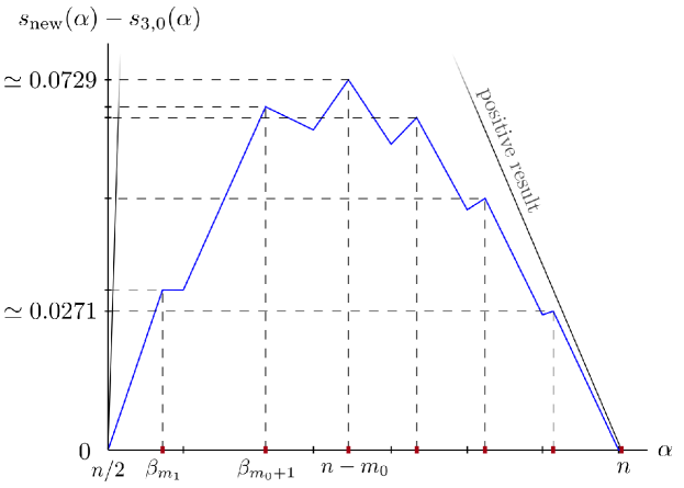
Figure 1. Representation of Theorem 1.1 for $n=15$, where we show the improvement with respect to the former lower bound (8). The positive result refers to Theorem 2.3 in [14].

In the notation of Theorem 1.1, the best previous result in [22] is

$$s_{c}(\alpha)\geq s_{3,0}(\alpha)\qquad\textrm{for }n/2\leq\alpha\leq n.$$ (18)

See Figure 1 for a graphical comparison between the old and the new results.

The counterexamples combine the fractal extension of Bourgain’s counterexample as presented in [22], and the intermediate space trick of Du–Kim–Wang–Zhang [13]. In [11], Du exploited this trick to construct counterexamples for (7), which are morally equivalent to counterexamples for convergence, except for one essential thing: for convergence the weight $w$ must intersect every line $t\mapsto(x,t)$ in at most one interval of length $1$. This additional restriction is evident in the fact that Bourgain’s counterexample needs Gauss sums, while Du’s examples do not. The contribution of this paper thus is to confirm that the numerology in Theorem 1.2 of [11] also holds for convergence.

Unlike Du, we want to construct a fractal divergence set, which demands further precautions. As we did in [16], we compute the dimension of this set using the Mass Transference Principle proved in [32] (see also [3]).

To compare Theorem 1.1 with Du’s Theorem 1.2 in [11], the reader can use the relationship

$$s_{i,m}(\alpha)=\frac{n-\alpha+1}{2}-\kappa_{i}(m+1;\alpha,n+1),$$ (19)

where $\kappa_{i}$ are functions defined by Du. Notice that we chose our notation trying to make it easier to compare our results with those of Du. The following dictionary might help:

Du’s Theorem 1.2	Theorem 1.1
$d$	$n+1$
$j$	$m+1$
$\kappa_{3}(j;\alpha,d)=\dfrac{d-j/2-\alpha}{d-j+1}$	$s_{3,m}(\alpha)$
$\kappa_{4}(j;\alpha,d)=\dfrac{d-\alpha}{2(d-j+1)}$	$s_{4,m}(\alpha)$
$\kappa_{5}(j;\alpha,d)=\dfrac{d-\alpha-1}{2(d-j-1)}$	$s_{5,m}(\alpha)$

Outline of the paper

1. For each integer $0\leq m\leq n-1$ we construct a family of counterexamples, where $m$ is the dimension associated with the “intermediate space trick”. We determine the set of divergence and the regularity of the initial data.

2. We use the Mass Transference Principle to compute the Hausdorff dimension of the set of divergence.

3. For each intermediate space dimension $m$ and the corresponding family of initial data, we fix a dimension $\alpha$ and identify the data with maximum regularity.

4. For a fixed dimension $\alpha$, we determine the maximum regularity among data with different $m$.

Notation

• We denote $e(z)=e^{2\pi iz}$, and the Fourier transform of $f$ and the solution $e^{it\Delta}f$ are

  $$\widehat{f}(\xi)=\int_{\mathbb{R}^{n}}f(x)\,e\big{(}-x\xi\big{)}\,dx\qquad\text{ and }\qquad e^{it\Delta}f(x)=\int_{\mathbb{R}^{n}}\widehat{f}(\xi)\,e\big{(}x\xi+t|\xi|^{2}\big{)}\,d\xi$$ (20)

• $B(a,r)=\{x:\lvert x-a\rvert\leq r\}$.

• $A\lesssim B$ means that $A\leq CB$ for some constant $C>0$. By $A\gtrsim B$ we denote the analog inequality. We write $A\simeq B$ if $A\lesssim B$ and $B\lesssim A$. When we want to stress some dependence of $C$ on a parameter $N$, we write $A\lesssim_{N}B$.

• We write $c\ll 1$ as a shorthand of “a sufficiently small constant”.

• Size of sets: If $E\subset\mathbb{R}^{n}$ is a Lebesgue measurable set, then either $\lvert E\rvert$ or $\mathcal{H}^{n}(E)$ denote its Lebesgue measure. If $E$ is a finite set, then $\lvert E\rvert$ is the number of elements.

• Given $0\leq\alpha\leq n$ and $\delta>0$, the $(\alpha,\delta)$-Hausdorff content of $E\subset\mathbb{R}^{n}$ is

  $$\mathcal{H}_{\delta}^{\alpha}(E)=\inf\bigg{\{}\sum_{j=1}^{\infty}(\textrm{diam}\,U_{j})^{\alpha}\mid E\subset\bigcup_{j=1}^{\infty}U_{j}\quad\textrm{such that}\quad\textrm{diam}\,U_{j}<\delta\bigg{\}},$$ (21)

  and the $\alpha$-Hausdorff measure of $E$ is $\mathcal{H}^{\alpha}(E)=\lim_{\delta\to 0}\mathcal{H}^{\alpha}_{\delta}(E)$. The Hausdorff dimension of $E$ is $\operatorname{dim_{\mathcal{H}}}E=\inf\{\alpha\geq 0\mid\mathcal{H}^{\alpha}(F)=0\}$.

Funding

Daniel Eceizabarrena is supported by the Simons Foundation Collaboration Grant on Wave Turbulence (Nahmod’s Award ID 651469), and by the National Science Foundation under Grant No. DMS-1929284 while he was in residence at ICERM - Institute for Computational and Experimental Research in Mathematics in Providence, RI, during the Hamiltonian Methods in Dispersive and Wave Evolution Equations program. Felipe Ponce-Vanegas is funded by the Basque Government through the BERC 2018-2021 program; by the Spanish State Research Agency through BCAM Severo Ochoa excellence accreditation SEV-2017-0718 and the project PGC2018-094528-B-I00 - IHAIP; and by a Juan de la Cierva – Formation grant FJC2019-039804-I.

Acknowledgments

We thank Renato Lucà for sharing with us all his insights on the problem. We also thank Alex Barron; the idea for this project arose after an email exchange with him.

2. Counterexample

Let $1\leq m\leq n-1$, and split the variable $\xi\in\mathbb{R}^{n}$ as

$$\xi=(\xi_{1},\xi^{\prime},\xi^{\prime\prime}),\qquad\text{ where }\qquad(\xi_{1},\xi^{\prime},\xi^{\prime\prime})\in\mathbb{R}\times\mathbb{R}^{n-m-1}\times\mathbb{R}^{m}.$$ (22)

Everywhere in this article, we use this notation for any variable in $\mathbb{R}^{n}$ or $\mathbb{Z}^{n}$. Let $\phi\in\mathcal{S}(\mathbb{R})$, $\varphi_{1}\in\mathcal{S}(\mathbb{R}^{n-m-1})$ and $\varphi_{2}\in\mathcal{S}(\mathbb{R}^{m})$, all of which have positive Fourier transform with support in a ball $B(0,c)$, for $c\ll 1$. Let also $\psi\in\mathcal{S}(\mathbb{R}^{n-m-1})$ be a cutoff function supported in $B(0,c)$, for $c\ll 1$. Let $R\gg 1$ be the scale of the counterexample, which we should think of as tending to infinity, and $D_{1},D_{2}\gg 1$ be parameters, which eventually will be appropriately chosen powers of $R$.

First, in Subsection 2.1 we construct a preliminary datum $f_{R}$ linked to a scale $R$. Then, in Subsection 2.2 we sum $f_{R}$ for dyadic $R$ to construct the counterexample for the convergence problem.

2.1. A preliminary initial datum

Let us first define the initial datum

$$f(x)=f_{R}(x)=g(x_{1})\,h_{1}(x^{\prime})\,h_{2}(x^{\prime\prime})$$ (23)

such that

$$\widehat{g}(\xi_{1})=\widehat{\phi}\left(\frac{\xi_{1}-R}{R^{1/2}}\right)$$ (24)

and

$$\widehat{h_{1}}(\xi^{\prime})=\sum_{\ell^{\prime}\in\mathbb{Z}^{n-m-1}}\,\psi\left(\frac{\ell^{\prime}}{R/D_{1}}\right)\,\widehat{\varphi}_{1}(\xi^{\prime}-D_{1}\,\ell^{\prime}),\qquad\qquad\widehat{h_{2}}(\xi^{\prime\prime})=\sum_{\begin{subarray}{c}\ell^{\prime\prime}\in\mathbb{Z}^{m}\\ |\ell^{\prime\prime}|\leq cR^{1/2}/D_{2}\end{subarray}}\,\widehat{\varphi}_{2}(\xi^{\prime\prime}-D_{2}\,\ell^{\prime\prime}).$$ (25)

Direct computation shows that

$$\left\lVert g\right\rVert_{2}\simeq R^{1/4},\qquad\left\lVert h_{1}\right\rVert_{2}\simeq\left(\frac{R}{D_{1}}\right)^{(n-m-1)/2},\qquad\left\lVert h_{2}\right\rVert_{2}\simeq\bigg{(}\frac{R^{1/2}}{D_{2}}\bigg{)}^{m/2},$$ (26)

so

$$\left\lVert f_{R}\right\rVert_{2}\simeq R^{1/4}\,\left(\frac{R}{D_{1}}\right)^{(n-m-1)/2}\,\bigg{(}\frac{R^{1/2}}{D_{2}}\bigg{)}^{m/2}.$$ (27)

Let us now study the evolution of this datum. We first do formal computations, which will be justified later.

• In the variable $x_{1}$,

  $$\left|e^{it\Delta}g(x_{1})\right|=R^{1/2}\,\left|\int_{\mathbb{R}}\widehat{\phi}(\xi_{1})\,e\left(\xi_{1}R^{1/2}(x_{1}+2tR)+tR|\xi_{1}|^{2}\right)\,d\xi_{1}\right|.$$ (28)

  If $|t|<1/R$ and $R^{1/2}|x_{1}+2Rt|<1$, we get

  $$\left|e^{it\Delta}g(x_{1})\right|\simeq R^{1/2}\,\phi(R^{1/2}(x_{1}+2Rt))\simeq R^{1/2}.$$ (29)

• For $x^{\prime\prime}$, we have

  $$e^{it\Delta}h_{2}(x^{\prime\prime})=\sum_{\begin{subarray}{c}\ell^{\prime\prime}\in\mathbb{Z}^{m}\\ |\ell^{\prime\prime}|\leq cR^{1/2}/D_{2}\end{subarray}}\,e^{2\pi i\left(D_{2}x^{\prime\prime}\cdot\ell^{\prime\prime}+tD_{2}^{2}\,|\ell^{\prime\prime}|^{2}\right)}\,\int_{\mathbb{R}^{m}}\widehat{\varphi}_{2}(\xi^{\prime\prime})\,e\big{(}\xi^{\prime\prime}(x^{\prime\prime}+2tD_{2}\ell^{\prime\prime})+t|\xi^{\prime\prime}|^{2}\big{)}\,d\xi^{\prime\prime}.$$ (30)

  The idea here is that if $|t|<1/R$ and if we restrict the variable to $|x^{\prime\prime}|<1$, all elements in the phase except $D_{2}x^{\prime\prime}\cdot\ell^{\prime\prime}$ are small. Thus,

  $$\left|e^{it\Delta}h_{2}(x^{\prime\prime})\right|\simeq\Big{|}\sum_{\begin{subarray}{c}\ell^{\prime\prime}\in\mathbb{Z}^{m}\\ |\ell^{\prime\prime}|\leq cR^{1/2}/D_{2}\end{subarray}}\,e^{2\pi i\,D_{2}x^{\prime\prime}\cdot\ell^{\prime\prime}}\Big{|}$$ (31)

  If we choose $x^{\prime\prime}=p^{\prime\prime}/D_{2}+\epsilon^{\prime\prime}$ for any $p^{\prime\prime}\in\mathbb{Z}^{m}$ and $|\epsilon^{\prime\prime}|<R^{-1/2}$, then

  $$\left|e^{it\Delta}h_{2}(x^{\prime\prime})\right|\simeq\left(\frac{R^{1/2}}{D_{2}}\right)^{m}.$$ (32)

• For $x^{\prime}$, $h_{1}$ has a similar structure as $h_{2}$, so we obtain

  $$e^{it\Delta}h_{1}(x^{\prime})=\sum_{\ell^{\prime}\in\mathbb{Z}^{n-m-1}}\,\psi\left(\frac{\ell^{\prime}}{R/D_{1}}\right)\,e^{2\pi i\left(D_{1}x^{\prime}\cdot\ell^{\prime}+tD_{1}^{2}\,|\ell^{\prime}|^{2}\right)}\,\int_{\mathbb{R}^{n-m-1}}\widehat{\varphi}_{1}(\xi^{\prime})\,e\left(\xi^{\prime}(x^{\prime}+2tD_{1}\ell^{\prime})+t|\xi^{\prime}|^{2}\right)\,d\xi^{\prime}.$$ (33)

  Again, restricting to $|x^{\prime}|<1$, the phase inside the integral is small, so we expect to have

  $$\left|e^{it\Delta}h_{1}(x^{\prime})\right|\simeq\Big{|}\sum_{\begin{subarray}{c}\ell^{\prime}\in\mathbb{Z}^{n-m-1}\\ |\ell^{\prime}|\leq cR/D_{1}\end{subarray}}\,e^{2\pi i\left(D_{1}x^{\prime}\cdot\ell^{\prime}+tD_{1}^{2}\,|\ell^{\prime}|^{2}\right)}\Big{|}.$$ (34)

  In this case we have a quadratic phase, so we take $x^{\prime}=p^{\prime}/(D_{1}\,q)+\epsilon^{\prime}$ and $t=p_{1}/(D_{1}^{2}q)$ such that $q\in 2\mathbb{N}+1$, $p_{1}\in\mathbb{Z}$ coprime with $q$, $p^{\prime}\in\mathbb{Z}^{n-m-1}$ and $|\epsilon^{\prime}|<R^{-1}$. That way, the exponential sum turns into the well-known Gauss sum, so we would obtain

  $$\begin{split}\left|e^{it\Delta}h_{1}(x^{\prime})\right|&\simeq\Big{|}\sum_{\begin{subarray}{c}\ell^{\prime}\in\mathbb{Z}^{n-m-1}\\ |\ell^{\prime}|\leq cR/D_{1}\end{subarray}}\,e\Big{(}\frac{p^{\prime}\cdot\ell^{\prime}+p_{1}\,|\ell^{\prime}|^{2}}{q}\Big{)}\Big{|}=\prod_{i=2}^{n-m}\Big{|}\sum_{n=-cR/D_{1}}^{cR/D_{1}}\,e\Big{(}\frac{p_{i}n+p_{1}\,n^{2}}{q}\Big{)}\Big{|}\\ &\simeq\prod_{i=2}^{n-m}\frac{R}{qD_{1}}\,\sqrt{q}=\left(\frac{R}{D_{1}\,q^{1/2}}\right)^{n-m-1}.\end{split}$$ (35)

Thus, combining (29), (32) and (35) we expect to obtain

$$\left|e^{it\Delta}f_{R}(x)\right|\simeq R^{1/2}\,\left(\frac{R}{D_{1}\,q^{1/2}}\right)^{n-m-1}\,\bigg{(}\frac{R^{1/2}}{D_{2}}\bigg{)}^{m},$$ (36)

subject to the restrictions

$$t=\frac{p_{1}}{D_{1}^{2}\,q},\quad x_{1}\in B^{1}\left(\frac{R}{D_{1}^{2}}\frac{p_{1}}{q},\frac{1}{R^{1/2}}\right),\quad x^{\prime}\in B^{n-m-1}\left(\frac{p^{\prime}}{D_{1}\,q},\frac{1}{R}\right),\quad x^{\prime\prime}\in B^{m}\left(\frac{p^{\prime\prime}}{D_{2}},\frac{1}{R^{1/2}}\right),$$ (37)

where $q\in 2\,\mathbb{N}+1$ and $p\in\mathbb{Z}^{n}$ such that $\operatorname{gcd}(p_{1},q)=1$. In view of this, let us define the slabs

$$E_{R}(p,q)=B^{1}\left(\frac{R}{D_{1}^{2}}\frac{p_{1}}{q},\frac{1}{R^{1/2}}\right)\times B^{n-m-1}\left(\frac{p^{\prime}}{D_{1}\,q},\frac{1}{R}\right)\times B^{m}\left(\frac{p^{\prime\prime}}{D_{2}},\frac{1}{R^{1/2}}\right).$$ (38)

All these formal computations, together with (27), motivate the following proposition:

Proposition 2.1.

Let $1\leq m\leq n-1$, $R\gg 1$ and $D_{1},D_{2},Q\gg 1$. Let $q\in 2\mathbb{N}+1$ be such that $Q/2\leq q<Q$ and $p\in\mathbb{Z}^{n}$ such that $\operatorname{gcd}(p_{1},q)=1$. Then, letting $t=p_{1}/(D_{1}^{2}q)$, we have

$$\frac{\left|e^{it\Delta}f_{R}(x)\right|}{\lVert f_{R}\rVert_{2}}\simeq R^{1/4}\,\left(\frac{R}{D_{1}Q}\right)^{(n-m-1)/2}\,\left(\frac{R^{1/2}}{D_{2}}\right)^{m/2},\qquad\forall x\in E_{R}(p,q).$$ (39)

Moreover, if $1/10\leq|x_{1}|\leq 1$, then the time satisfies $t\simeq 1/R$.

Proof.

Let us first check that $t\simeq 1/R$. Indeed, from the definition of $E_{R}(p,q)$, we have $x_{1}\in B(Rt,R^{-1/2})$, which implies

$$1/20\leq x_{1}-R^{-1/2}\leq Rt\leq x_{1}+R^{-1/2}\leq 2,$$ (40)

if $R$ is large enough.

The main estimate (39) follows by combining (29), (32) and (35) with (27). Thus, it suffices to justify (29), (32) and (35).

Estimate (29) follows from direct computation. Indeed, from (28) we write

$$\left|e^{it\Delta}g(x_{1})\right| =R^{1/2}\,\left|\int_{\mathbb{R}}\widehat{\phi}(\xi_{1})\,e\left(\xi_{1}R^{1/2}(x_{1}+2tR)+tR|\xi_{1}|^{2}\right)\,d\xi_{1}\right|$$ (41)

$$\geq R^{1/2}\bigg{\lvert}\int_{\mathbb{R}}\widehat{\phi}(\xi_{1})\,\cos\big{(}2\pi\big{(}\xi_{1}R^{1/2}(x_{1}+2tR)+tR|\xi_{1}|^{2}\big{)}\big{)}\,d\xi_{1}\bigg{\rvert}.$$ (42)

Asking $\lvert R^{1/2}(x_{1}+2tR)\rvert<1$ and $\lvert tR\rvert<1$, since $\operatorname{supp}\widehat{\phi}\subset[-c,c]$ for $c$ small enough, we get

$$\Big{|}\xi_{1}R^{1/2}(x_{1}+2tR)+tR|\xi_{1}|^{2}\Big{|}<1/10,$$ (43)

and therefore $|e^{it\Delta}g(x_{1})|\gtrsim R^{1/2}$.

We prove (32) similarly. From (30) we have

$$e^{it\Delta}h_{2}(x^{\prime\prime})=\int_{\mathbb{R}^{m}}\widehat{\varphi}_{2}(\xi^{\prime\prime})\,\sum_{\begin{subarray}{c}\ell^{\prime\prime}\in\mathbb{Z}^{m}\\ |\ell^{\prime\prime}|\leq cR^{1/2}/D_{2}\end{subarray}}\,e\Big{(}D_{2}x^{\prime\prime}\cdot\ell^{\prime\prime}+tD_{2}^{2}\,|\ell^{\prime\prime}|^{2}+\xi^{\prime\prime}(x^{\prime\prime}+2tD_{2}\ell^{\prime\prime})+t|\xi^{\prime\prime}|^{2}\Big{)}\,d\xi^{\prime\prime}.$$ (44)

Let $x^{\prime\prime}=p^{\prime\prime}/D_{2}+\epsilon^{\prime\prime}$ with $|\epsilon^{\prime\prime}|\leq R^{-1/2}$. Since $\operatorname{supp}\widehat{\varphi}_{2}\subset[-c,c]$, choosing $c$ small enough we get

$$\Big{|}D_{2}\epsilon^{\prime\prime}\cdot\ell^{\prime\prime}+tD_{2}^{2}\,|\ell^{\prime\prime}|^{2}+\xi^{\prime\prime}(x^{\prime\prime}+2tD_{2}\ell^{\prime\prime})+t|\xi^{\prime\prime}|^{2}\Big{|}<1/10,$$ (45)

and thus $\lvert e^{it\Delta}h_{2}(x^{\prime\prime})\rvert\gtrsim(R^{1/2}/D_{2})^{m}$.

Estimate (35) is more technical. Let $x^{\prime}=p^{\prime}/(D_{1}q)+\epsilon^{\prime}$ with $|\epsilon^{\prime}|<R^{-1}$, and write

$$\big{\lvert}e^{it\Delta}h_{1}(x^{\prime})\big{\rvert}=\Big{\lvert}\sum_{\ell^{\prime}\in\mathbb{Z}^{n-m-1}}\,\zeta(\ell^{\prime})\,e\Big{(}\frac{p^{\prime}\cdot\ell^{\prime}+p_{1}|\ell^{\prime}|^{2}}{q}\Big{)}\Big{\rvert},$$ (46)

where

$$\zeta(\ell^{\prime})=\psi\left(\frac{\ell^{\prime}}{R/D_{1}}\right)\,e^{2\pi iD_{1}\epsilon^{\prime}\cdot\ell^{\prime}}\,\int\widehat{\varphi}_{1}(\xi^{\prime})\,e\left(\xi^{\prime}(x^{\prime}+2tD_{1}\ell^{\prime})+t|\xi^{\prime}|^{2}\right)\,d\xi^{\prime}.$$ (47)

To bound (46), we use a simplified version of [16, Lemma 3.4].

Lemma 2.2 (Lemma 3.4 of [16]).

Let $d\in\mathbb{N}$ and $f(m)=a\,|m|^{2}+b\cdot m$ such that $a\in\mathbb{Z}$ and $b\in\mathbb{Z}^{d}$. Let also $\zeta\in C_{0}^{\infty}(\mathbb{R}^{d})$ and define the discrete Laplacian $\widetilde{\Delta}$ by

$$\widetilde{\Delta}\zeta(y)=\sum_{j=1}^{d}\big{(}\zeta(y+e_{j})+\zeta(y-e_{j})-2\zeta(y)\big{)},\qquad y\in\mathbb{R}^{d},$$ (48)

where $(e_{j})_{j=1}^{d}$ is the canonical basis of $\mathbb{R}^{d}$. Assume that $\zeta$ is supported in $B(0,L)$ for some $L>0$, and moreover that $\lVert\widetilde{\Delta}^{N}\zeta\rVert_{\infty}\lesssim_{N}L^{-2N}$ for every $N\in\mathbb{N}$. Then,

$$\sum_{m\in\mathbb{Z}^{d}}\zeta(m)\,e\Big{(}\frac{f(m)}{q}\Big{)}=\bigg{(}\frac{1}{q^{d}}\sum_{m\in\mathbb{Z}^{d}}\zeta(m)\bigg{)}\sum_{l\in\mathbb{Z}_{q}^{d}}e\Big{(}\frac{f(l)}{q}\Big{)}+\operatorname{\mathcal{O}}_{N}\bigg{(}q^{d/2}\left(\frac{L}{q}\right)^{d-2N}\bigg{)}$$ (49)

for any integer $N>d/2$.

We use the lemma with $d=n-m-1$ and $L=R/D_{1}$. Rewrite $\zeta$ in (47) as

$$\zeta(\ell^{\prime})=\psi\left(\frac{\ell^{\prime}}{L}\right)\,e^{2\pi i\delta\,\cdot\ell^{\prime}/L}\,\int\widehat{\varphi}_{1}(\xi^{\prime})\,e\left(\xi^{\prime}(x^{\prime}+2\tau\ell^{\prime}/L)+t|\xi^{\prime}|^{2}\right)\,d\xi^{\prime},$$ (50)

where $\delta=R\epsilon^{\prime}$ and $\tau=Rt$ satisfy $|\delta|,|\tau|<1$. Notice that $\zeta$ is supported in $B(0,L)$. On the other hand, we have $\lVert\widetilde{\Delta}^{N}\zeta\rVert_{\infty}\lesssim\sup_{|\alpha|=2N}\lVert\partial^{\alpha}\zeta\rVert_{\infty}$, where $\alpha=(\alpha_{2},\ldots,\alpha_{n-m})$ denotes a multi-index. Thus, it suffices to bound $\lVert\partial^{\alpha}\zeta\rVert_{\infty}$ uniformly in $x^{\prime}$ and $t$. Write

$$\partial^{\alpha}\zeta(y)=\int\widehat{\varphi}_{1}(\xi^{\prime})\,e^{2\pi i\left(\xi^{\prime}\cdot x^{\prime}+t|\xi^{\prime}|^{2}\right)}\,\partial^{\alpha}\Big{[}\psi\left(\frac{y}{L}\right)\,e^{2\pi i(\delta+2\tau\xi^{\prime})\cdot y/L}\Big{]}\,d\xi^{\prime},\qquad y\in\mathbb{R}^{n-m-1},\,\,|y|\leq L.$$ (51)

Calling $A(z)=\psi(z)\,e^{2\pi i(\delta+2\tau\xi^{\prime})\cdot z}$, we have

$$\partial^{\alpha}\Big{[}\psi\left(\frac{y}{L}\right)\,e^{2\pi i\,(\delta+2\tau\xi^{\prime})\cdot y/L}\Big{]}=\frac{1}{L^{2N}}\,\partial^{\alpha}A(y/L),$$ (52)

and since $\partial^{\alpha}A(z)$ is uniformly bounded in $|\delta|,|\tau|,|z|<1$, we get $\lVert\partial^{\alpha}\zeta\rVert_{\infty}\lesssim_{N}L^{-2N}$. Thus, by Lemma 2.2, we estimate (46) as

$$\begin{split}\Big{|}e^{it\Delta}h_{1}(x^{\prime})\Big{|}&=\frac{1}{q^{n-m-1}}\,\Big{|}\sum_{\ell^{\prime}\in\mathbb{Z}^{n-m-1}}\zeta(\ell^{\prime})\Big{|}\,\Big{|}\sum_{\ell^{\prime}\in\mathbb{Z}_{q}^{n-m-1}}\,e\Big{(}\frac{p^{\prime}\cdot\ell^{\prime}+p_{1}|\ell^{\prime}|^{2}}{q}\Big{)}\,\Big{|}\\ &\qquad\qquad\qquad\qquad\qquad\qquad\qquad\qquad\qquad+\mathcal{O}_{N}\left(q^{(n-m-1)/2}\,\bigg{(}\frac{L}{q}\right)^{n-m-1-2N}\bigg{)}.\end{split}$$ (53)

Since the phase of $\zeta$ in (50) is small, by the same procedure we used for (32) we get

$$\Big{|}\sum_{\ell^{\prime}\in\mathbb{Z}^{n-m-1}}\zeta(\ell^{\prime})\Big{|}\simeq L^{n-m-1}.$$ (54)

Also, since $\operatorname{gcd}(p_{1},q)=1$, $q$ is odd and $q\simeq Q$, the Gauss sums in (53) satisfy

$$\Big{|}\sum_{\ell^{\prime}\in\mathbb{Z}_{q}^{n-m-1}}\,e\left(\frac{p^{\prime}\cdot\ell^{\prime}+p_{1}|\ell^{\prime}|^{2}}{q}\right)\,\Big{|}\simeq Q^{(n-m-1)/2}.$$ (55)

Thus, taking $N>(n-m-1)/2$ and replacing $L=R/D_{1}$, from (53) we get

$$\begin{split}\Big{|}e^{it\Delta}h_{1}(x^{\prime})\Big{|}&\simeq Q^{(n-m-1)/2}\left(\frac{L}{Q}\right)^{n-m-1}+\mathcal{O}_{N}\bigg{(}Q^{(n-m-1)/2}\,\Big{(}\frac{L}{Q}\Big{)}^{n-m-1-2N}\bigg{)}\\ &\gtrsim Q^{(n-m-1)/2}\left(\frac{L}{Q}\right)^{n-m-1}\\ &=\left(\frac{R}{D_{1}Q^{1/2}}\right)^{n-m-1},\end{split}$$ (56)

which proves (35). ∎

Roughly speaking, Proposition 2.1 would suffice in the case of the Lebesgue measure $\alpha=n$. Indeed, given that $Q$, $D_{1}$ and $D_{2}$ will be certain powers of $R$, we will be able to find an exponent $s_{m}=s_{m}(Q,D_{1},D_{2})$ such that

$$\frac{\left|e^{it\Delta}f_{R}(x)\right|}{\lVert f_{R}\rVert_{2}}\simeq R^{1/4}\,\left(\frac{R}{D_{1}Q}\right)^{(n-m-1)/2}\,\bigg{(}\frac{R^{1/2}}{D_{2}}\bigg{)}^{m/2}=R^{s_{m}},\qquad\forall x\in E_{R}(p,q).$$ (57)

Since the estimate does not depend on the particular choice of $p,q$ but rather on the size $q\simeq Q$, then (58) holds for $F_{R}=\bigcup_{q\simeq Q}\bigcup_{p}E_{R}(p,q)$. Consequently, up to checking that $\mathcal{H}^{n}(F_{R}\cap B(0,1))\simeq 1$ for all $R$, we would be able to write

$$\frac{\left\lVert\sup_{t}\left|e^{it\Delta}f_{R}\right|\right\rVert_{L^{2}(B(0,1))}}{\lVert f_{R}\rVert_{H^{s_{m}-\epsilon}}}\gtrsim R^{\epsilon},\qquad\forall R\gg 1,$$ (58)

which would disprove the standard maximal estimate, which is equivalent to the almost everywhere convergence property, in $H^{s}(\mathbb{R}^{n})$ for all $s<s_{m}$.

However, in the fractal case $\alpha<n$, where we ask for almost everywhere convergence with respect to the $\mathcal{H}^{\alpha}$ measure, the maximal characterization does not work. This means that we need to construct a divergent counterexample explicitly.

2.2. Construction of the counterexample

Let $\alpha<n$. To find a counterexample for the $\mathcal{H}^{\alpha}$ almost everywhere convergence property, we need to construct a function $f\in H^{s}(\mathbb{R}^{n})$ whose set of divergence $F$ satisfies $\operatorname{dim}_{\mathcal{H}}F=\alpha$. Moreover, we look for the biggest possible Sobolev regularity $s$.

The standard way to do this is to sum dyadically the data $f_{R}$ we constructed in the previous section. For every $j\in\mathbb{N}$, let $R_{j}=2^{j}$. As before, assume that $Q$, $D_{1}$ and $D_{2}$ are powers of $R$ so that $s_{m}=s_{m}(Q,D_{1},D_{2})$ is well-defined in (57). Define

$$f(x)=\sum_{j\geq K_{0}}\,j\,\frac{f_{R_{j}}(x)}{R_{j}^{s_{m}}\,\lVert f_{R_{j}}\rVert_{2}}$$ (59)

for some $K_{0}$ large enough. Observe that $f\in H^{s}(\mathbb{R}^{n})$ for every $s<s_{m}$ because

$$\lVert f\rVert_{H^{s}}\leq\sum_{j\geq K_{0}}j\frac{\lVert f_{R_{j}}\rVert_{H^{s}}}{R_{j}^{s_{m}}\,\lVert f_{R_{j}}\rVert_{2}}\simeq\sum_{j\geq K_{0}}\frac{j}{R_{j}^{s_{m}-s}}<\infty.$$ (60)

As suggested at the end of the previous subsection, since the estimate in Proposition 2.1 does not depend on $p,q$ but only on $Q$, we work with

$$F_{k}=\bigcup_{\begin{subarray}{c}Q_{k}/2\leq q<Q_{k}\\ q\in 2\mathbb{N}+1\end{subarray}}\,\,\bigcup_{p\in G(q)}E_{k}(p,q),$$ (61)

where we denote $E_{k}(p,q)=E_{R_{k}}(p,q)$ and $G(q)=\left\{p\in\mathbb{Z}^{n}\,:\,\operatorname{gcd}(p_{1},q)=1\right\}$. This way, by Proposition 2.1 we have

$$\frac{\big{|}e^{it\Delta}f_{R_{k}}(x)\big{|}}{R_{k}^{s_{m}}\,\lVert f_{R_{k}}\rVert_{2}}\simeq 1,\qquad\forall x\in F_{k},\qquad\forall k\in\mathbb{N}$$ (62)

However, this only accounts for the behavior of the piece $f_{R_{k}}$. We show next that the contribution of the remaining $f_{R_{j}}$ with $j\neq k$ is much smaller.

Proposition 2.3.

Let $K_{0}\in\mathbb{N}$ be large enough and $k\geq K_{0}$. Let $x\in F_{k}\cap B(0,1)$ be such that $1/10<|x_{1}|\leq 1$. Then, there exists a time $t=t(x)\simeq R_{k}^{-1}$ such that $\big{\lvert}e^{it(x)\Delta}f(x)\big{\rvert}\gtrsim k.$

With this proposition, the construction of the counterexample will be concluded if we can take the limit $k\to\infty$. For that, we need points that lie in infinitely many sets $F_{k}$. The set of divergence is thus

$$F=\limsup_{k\to\infty}F_{k}=\bigcap_{K\in\mathbb{N}}\bigcup_{k\geq K}F_{k}.$$ (63)

Corollary 2.4.

Let $F=\limsup_{k\to\infty}F_{k}$. Then,

$$\limsup_{t\to 0}\big{|}e^{it\Delta}f(x)\big{|}=\infty,\qquad\forall x\in F\cap A(1/10,1).$$ (64)

Proof of Corollary 2.4.

If $x\in F$, then there exists a sequence $k_{n}$ such that $x\in F_{k_{n}}$ for all $n\in\mathbb{N}$. By Proposition 2.3, there exists a sequence of times $t_{n}=t_{n}(x)$ such that $t_{n}\simeq 1/R_{k_{n}}$ and $|e^{it_{n}\Delta}f(x)|\gtrsim k_{n}$ for all $n\in\mathbb{N}$. Thus, since $\lim_{n\to\infty}t_{n}(x)=0$, we get

$$\limsup_{t\to 0}\big{|}e^{it\Delta}f(x)\big{|}\geq\lim_{n\to\infty}\big{|}e^{it_{n}(x)\Delta}f(x)\big{|}=\infty.$$ (65)

∎

In view of Corollary 2.4, the main goal turns to computing the Hausdorff dimension of $F$. We do that in Section 3. To conclude this section, we prove Proposition 2.3.

Proof of Proposition 2.3.

Fix $k\geq K_{0}$ and take $x\in F_{k}$. According to (59), the solution looks like

$$\sum_{j\geq K_{0}}j\,\frac{e^{it\Delta}f_{R_{j}}(x)}{R_{j}^{s_{m}}\,\lVert f_{R_{j}}\rVert_{2}}.$$ (66)

We first focus on the contribution of the piece $e^{it\Delta}f_{R_{j}}$ with $j=k$. Since $x\in F_{k}$, there are $p_{1}$ and $q\simeq Q$ such that $x\in E_{R_{k}}(p,q)$, and thus, by Proposition 2.1, there is a time $t(x)=p_{1}/(D_{1}q)$ such that $t(x)\simeq 1/R_{k}$ and

$$\frac{\big{|}e^{it(x)\Delta}f_{R_{k}}(x)\big{|}}{R_{k}^{s_{m}}\,\lVert f_{R_{k}}\rVert_{2}}\simeq 1.$$ (67)

Now we want to measure the contribution of $e^{it(x)\Delta}f_{j}(x)$ for $j\neq k$. We are going to prove

$$\frac{\big{|}e^{it(x)\Delta}f_{R_{j}}(x)\big{|}}{R_{j}^{s_{m}}\,\lVert f_{R_{j}}\rVert_{2}}\lesssim\frac{1}{j\,R_{j}},\qquad\forall j\neq k.$$ (68)

If this holds, then joining (67) and (68) we get

$$\big{|}e^{it(x)\Delta}f(x)\big{|}\gtrsim k-C\sum_{j\neq k}\frac{1}{R_{j}}\geq k-C\sum_{j=1}^{\infty}\frac{1}{2^{j}}\geq k/2,\qquad\text{for }K_{0}\gg 1,$$ (69)

which would conclude the proof.

To prove (68), the idea is that the term $e^{it\Delta}g_{R_{j}}(x_{1})$ in (29) localizes the solution to the $n$-plane $T_{j}=\{x\,:\,|x_{1}+2R_{j}t|<R_{j}^{1/2}\}$. Thus, if $j\neq k$, the planes $T_{j}$ and $T_{k}$ are disjoint except in a neighborhood of the origin. Consequently, if $|x_{1}|>1/10$, the contribution of $e^{it\Delta}g_{R_{j}}(x_{1})$ in the plane $T_{k}$ is very small.

Let us formalize the previous paragraph. First, we directly bound the contribution in the variables $x^{\prime}$ and $x^{\prime\prime}$. From (30) and (35), we get

$$\big{|}e^{it\Delta}h_{1,R_{j}}(x^{\prime})\big{|}\lesssim\left(\frac{R_{j}}{D_{1}}\right)^{n-m-1}\qquad\text{ and }\qquad\big{|}e^{it\Delta}h_{2,R_{j}}(x^{\prime\prime})\big{|}\lesssim\bigg{(}\frac{R_{j}^{1/2}}{D_{2}}\bigg{)}^{m},$$ (70)

and thus

$$\big{|}e^{it\Delta}f_{R_{j}}(x)\big{|}\lesssim\frac{R_{j}^{n-m/2-1}}{D_{1}^{n-m-1}\,D_{2}^{m}}\,\big{|}e^{it\Delta}g_{R_{j}}(x_{1})\big{|}.$$ (71)

Now, from (28), write

$$\big{|}e^{it\Delta}g_{R_{j}}(x_{1})\big{|}=R_{j}^{1/2}\,\left|\int_{\mathbb{R}}\widehat{\phi}(\eta)\,e^{2\pi i\,\lambda_{j}\theta_{j}(\eta)}\,d\eta\right|$$ (72)

where

$$\lambda_{j}=R_{j}^{1/2}\,|x_{1}+2tR_{j}|,\qquad\theta_{j}(\eta)=\eta+\frac{t}{\lambda_{j}}\,R_{j}\,\eta^{2},\qquad\theta_{j}^{\prime}(\eta)=1+2\frac{tR_{j}}{\lambda_{j}}\,\eta.$$ (73)

Now we exploit the decay of this oscillatory integral. Observe that

$$\begin{split}\lambda_{j}&=R_{j}^{1/2}\,\Big{(}2t|R_{j}-R_{k}|+\mathcal{O}\left(|x_{1}+2tR_{k}|\right)\,\Big{)}\\ &\simeq R_{j}^{1/2}\,\Big{(}2\frac{|R_{j}-R_{k}|}{R_{k}}+\mathcal{O}\left(R_{k}^{-1/2}\right)\,\Big{)}.\end{split}$$ (74)

We separate in two cases:

• If $j<k$, then $R_{j}/R_{k}\leq 1/2$ and

  $$\lambda_{j}\simeq R_{j}^{1/2}\,\Big{(}1-\frac{R_{j}}{R_{k}}+\mathcal{O}\left(R_{k}^{-1/2}\right)\,\Big{)}\simeq R_{j}^{1/2}.$$ (75)

  In this case,

  $$\Big{|}\frac{tR_{j}}{\lambda_{j}}\eta\Big{|}\leq\frac{R_{j}}{R_{k}\,R_{j}^{1/2}}\leq\frac{1}{R_{j}^{1/2}}<\frac{1}{4}\qquad\Longrightarrow\qquad\left|\theta^{\prime}_{j}(\eta)\right|>1/2>0.$$ (76)

• If $j>k$, then $R_{j}/R_{k}\geq 2$ and

  $$\lambda_{j}\simeq R_{j}^{1/2}\,\Big{(}\frac{R_{j}}{R_{k}}-1+\mathcal{O}\left(R_{k}^{-1/2}\right)\,\Big{)}\simeq R_{j}^{1/2}\,\frac{R_{j}}{R_{k}}.$$ (77)

  In particular $\lambda_{j}>R_{j}^{1/2}$, so in this case

  $$\Big{|}\frac{tR_{j}}{\lambda_{j}}\eta\Big{|}\leq\frac{R_{j}}{R_{k}\,\lambda_{j}}\simeq\frac{1}{R_{j}^{1/2}}<\frac{1}{4}\qquad\Longrightarrow\qquad\left|\theta^{\prime}_{j}(\eta)\right|>1/2>0.$$ (78)

Thus, in both cases we can integrate by parts in (72) to obtain

$$\big{|}e^{it\Delta}g_{R_{j}}(x_{1})\big{|}\lesssim\frac{R_{j}^{1/2}}{\lambda_{j}^{N}}\lesssim\frac{1}{R_{j}^{(N-1)/2}},\qquad\forall N\in\mathbb{N}.$$ (79)

Coming back to (71), using (27) and recalling that $D_{1}$ and $D_{2}$ will be powers of $R$, we get

$$\frac{\big{|}e^{it(x)\Delta}f_{R_{j}}(x)\big{|}}{R_{j}^{s_{m}}\,\lVert f_{R_{j}}\rVert_{2}}\lesssim\frac{1}{R_{j}^{N}},\qquad\forall N\in\mathbb{N}.$$ (80)

In particular, we get (68) and the proof is complete. ∎

3. Dimension of the set of divergence

In this section we compute the Hausdorff dimension of the divergence set $F$ defined in (61) and (63). Recall that the slabs in (38) are

$$E_{R}(p,q)=B^{1}\bigg{(}\frac{R}{D_{1}^{2}}\,\frac{p_{1}}{q},\frac{1}{R^{1/2}}\bigg{)}\times B^{n-m-1}\bigg{(}\frac{1}{D_{1}}\frac{p^{\prime}}{q},\frac{1}{R}\bigg{)}\times B^{m}\bigg{(}\frac{p^{\prime\prime}}{D_{2}},\frac{1}{R^{1/2}}\bigg{)},$$ (81)

and that we build the divergence set with $E_{k}(p,q)=E_{R_{k}}(p,q)$. Rather than with the parameters $D_{1},D_{2}$ and $Q$, we find it more convenient to work with $(u_{1},u_{2},u_{3})$ defined by

$$R^{u_{1}}=\frac{QD_{1}^{2}}{R},\qquad R^{u_{2}}=QD_{1},\qquad\mbox{and}\qquad R^{u_{3}}=D_{2},$$ (82)

or equivalently,

$$Q=R^{2u_{2}-u_{1}-1},\qquad D_{1}=R^{1+u_{1}-u_{2}},\qquad\mbox{and}\qquad D_{2}=R^{u_{3}}.$$ (83)

In view of (81), $(u_{1},u_{2},u_{3})$ determine the separation of successive slabs for each fixed $q$ in the coordinates $x_{1},x^{\prime}$ and $x^{\prime\prime}$ respectively.

We have a few preliminary restrictions for the parameters. For each fixed $q$, we want that successive slabs do not intersect with each others. For that, for instance in $x_{1}$, we need

$$\frac{1}{R^{1/2}}<\frac{R}{D_{1}q}\simeq\frac{R}{D_{1}Q}=\frac{1}{R^{u_{1}}}\quad\Longrightarrow\quad u_{1}\leq 1/2.$$ (84)

Also, we require that we have more than a single slab in each of the directions, so we require $R^{-u_{1}}=R/(D_{1}Q)\ll 1$, which implies $u_{1}>0$. Similar reasons suggest that we require

$$0<u_{1}\leq 1/2,\qquad 0<u_{2}\leq 1\quad\text{ and }\quad 0<u_{3}\leq 1/2.$$ (85)

Since $Q$ is the size of the denominators $q\in\mathbb{N}$, we always have $Q\geq 1$, which implies

$$2u_{2}-u_{1}\geq 1.$$ (86)

3.1. Upper bound

With these restrictions, we can compute an upper bound for $\operatorname{dim_{\mathcal{H}}}F$.

Proposition 3.1.

Let $F\subset\mathbb{R}^{n}$ be the divergence set defined in (61) and (63), with parameters $(u_{1},u_{2},u_{3})$ as in (82), subject to the restrictions (85) and (86). Then,

$$\operatorname{dim_{\mathcal{H}}}F\leq\min\{\alpha_{1},\alpha_{2}\},$$ (87)

where

$$\alpha_{1}=\frac{m-1}{2}+(n-m+1)u_{2}+mu_{3}$$ (88)

and

$$\alpha_{2}=\begin{cases}n-m-3+4u_{2}+2mu_{3},&\text{for}\quad u_{2}\leq 3/4\\ n-m+2mu_{3},&\text{for}\quad u_{2}\geq 3/4\end{cases}$$ (89)

Proof.

Since $F=\limsup_{k\to\infty}F_{k}\subset\bigcup_{k\geq N}F_{k}$ for all $N>0$, it suffices to cover $F_{k}$ for every $k\in\mathbb{N}$. From the definition in (61), $F_{k}$ is formed by

$$Q\cdot R^{u_{1}}\cdot R^{(n-m-1)u_{2}}\cdot R^{mu_{3}}=R^{(n-m+1)u_{2}+mu_{3}-1}$$ (90)

slabs $E_{k}(p,q)$. Each of those slabs is covered by $R_{k}^{1/2}\,\big{(}R_{k}^{1/2}\big{)}^{m}$ balls of radius $R_{k}^{-1}$. In all, each $F_{k}$ is covered by

$$R^{(n-m+1)u_{2}+mu_{3}-1}\,R^{\frac{m+1}{2}}=R^{(n-m+1)u_{2}+mu_{3}+\frac{m-1}{2}},$$ (91)

so taking $\delta=R_{N}^{-1}$, we get

$$\mathcal{H}^{\alpha}_{R_{N}^{-1}}(F)\leq\sum_{k=N}^{\infty}R^{-\alpha}\,R^{(n-m+1)u_{2}+mu_{3}+\frac{m-1}{2}}.$$ (92)

Thus, if $\alpha\geq(n-m+1)u_{2}+mu_{3}+\frac{m-1}{2}=\alpha_{1}$, we get $\mathcal{H}^{\alpha}(F)=\lim_{N\to\infty}H^{\alpha}_{R_{N}^{-1}}(F)=0$, so $\operatorname{dim_{\mathcal{H}}}F\leq\alpha_{1}$.

To prove $\operatorname{dim_{\mathcal{H}}}F\leq\alpha_{2}$, we need to arrange the slabs of $F$ differently (see Figure 2 for visual support).

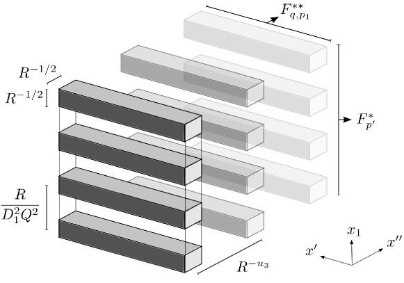
Figure 2. Arrangement of the slabs of $F_{k}$.

First, observe that in the direction $x^{\prime\prime}$ the slabs are disjoint. Thus, it is useful to arrange $F_{k}$ as

$$F_{k}=\bigcup_{p^{\prime\prime}\in\mathbb{Z}^{m}}\Bigg{[}\bigcup_{q\simeq Q}\bigcup_{(p_{1},p^{\prime})\in G(q)}E_{k}(p,q)\Bigg{]}=\bigcup_{p^{\prime\prime}\in\mathbb{Z}^{m}}F^{*}_{k,p^{\prime\prime}}.$$ (93)

Let us look at the separation between two slabs $E_{k}(p,q)$ and $E_{k}(\tilde{p},\tilde{q})$ in the direction $x_{1}$, which is

$$\frac{R}{D_{1}^{2}}\frac{|p_{1}\tilde{q}-\tilde{p}_{1}q|}{q\tilde{q}}\gtrsim\frac{R}{D_{1}^{2}Q^{2}}=R^{1-2u_{2}}.$$ (94)

Thus, if we ask $R^{1-2u_{2}}>R^{-1/2}$, which amounts to $u_{2}\leq 3/4$, the slabs in direction $x_{1}$ are disjoint. Consequently, we can further arrange

$$F^{*}_{k,p^{\prime\prime}}=\bigcup_{q\simeq Q}\bigcup_{p_{1}}\bigg{[}\bigcup_{p^{\prime}:p\in G(q)}E(p,q)\bigg{]}=\bigcup_{q\simeq Q}\bigcup_{p_{1}}F^{**}_{k,q,p_{1},p^{\prime\prime}},$$ (95)

and the number of sets $F^{**}_{k,q,p_{1},p^{\prime\prime}}$ in $F_{k}$ is at most $R^{2u_{2}-1}\,R^{m\,u_{3}}$. Since each set $F^{**}_{k,q,p_{1},p^{\prime\prime}}$ can be covered by an $R^{-1/2}_{k}$ neighborhood of a $(n-m-1)$-plane, in particular we can cover it by $R^{(n-m-1)/2}_{k}$ balls of radius $R^{-1/2}_{k}$. Thus,

$$\mathcal{H}_{R_{N}^{-1/2}}^{\alpha}(F)\leq\sum_{k=N}^{\infty}R_{k}^{-\alpha/2}\,R_{k}^{2u_{2}-1+mu_{3}+(n-m-1)/2},$$ (96)

so $\mathcal{H}^{\alpha}(F)=\lim_{N\to\infty}\mathcal{H}_{R_{N}^{-1/2}}^{\alpha}(F)=0$ if $\alpha\geq n-m-3+4u_{2}+2mu_{3}=\alpha_{2}$. Thus, $\operatorname{dim_{\mathcal{H}}}F\leq\alpha_{2}$.

When $u_{2}>3/4$, the slabs in direction $x_{1}$ need not be disjoint anymore. Still, from the arrangement (93), every $F_{k,p^{\prime\prime}}^{*}$ can be covered by a $R_{k}^{-1/2}$ neighborhood of a $(n-m)$-plane, which in turn is covered by $R_{k}^{(n-m)/2}$ balls of radius $R_{k}^{-1/2}$. Since there are $R_{k}^{mu_{3}}$ different $F_{k,p^{\prime\prime}}^{*}$ in $F_{k}$,

$$\mathcal{H}_{R_{N}^{-1/2}}^{\alpha}(F)\leq\sum_{k=N}^{\infty}R_{k}^{-\alpha/2}\,R_{k}^{mu_{3}+(n-m)/2}.$$ (97)

Thus, if $\alpha>n-m+2mu_{3}=\alpha_{2}$, we get $\mathcal{H}^{\alpha}(F)=\lim_{N\to\infty}\mathcal{H}_{R_{N}^{-1/2}}^{\alpha}(F)=0$, which implies $\operatorname{dim_{\mathcal{H}}}F\leq\alpha_{2}$. ∎

3.2. Lower bound

As we announced in the introduction, to prove the lower bound for $\operatorname{dim_{\mathcal{H}}}F$ we use the Mass Transference Principle from rectangles to rectangles proved by Wang and Wu [32]. For that, in the following lines we identify our setting with the notation and definitions introduced in [32, Section 3.1].

Let us index each slab $E_{k}(p,q)$ with $\alpha=(k,p,q)$ and gather the indices in

$$J=\bigcup_{k\gg 1}J_{k},$$ (98)

$$J_{k}=\{(k,p,q)\mid Q_{k}/2\leq q\textrm{ odd}\leq Q_{k}\textrm{ and }(p_{1},p^{\prime},p^{\prime\prime})\in G(q)\times\mathbb{Z}^{m}\}.$$ (99)

The resonant set $\{\mathcal{R}_{\alpha}\mid\alpha\in J\}$ from [32, Definition 3.1] corresponds to the set of centers of the slabs, so we work with $\kappa=0$. Define the function $\beta:J\to\mathbb{R}_{+}$ by $\beta((k,p,q))=R_{k}$, and we set $u_{k}=l_{k}=R_{k}$ so that $J_{k}=\{\alpha\mid l_{k}\leq\beta(\alpha)\leq u_{k}\}=\{\alpha\mid\beta(\alpha)=R_{k}\}$. Also, we set $\rho(u)=u^{-1}$, so our slabs can be rewritten as

$$E_{k}(p,q)=B(\mathcal{R}_{\alpha},\rho(R_{k}))^{\boldsymbol{b}}=\prod_{i=1}^{n}B\big{(}\mathcal{R}_{\alpha,i},\rho(R_{k})^{b_{i}}\big{)},$$ (100)

where the exponent $\boldsymbol{b}=(b_{1},\ldots,b_{n})$ is

$$\boldsymbol{b}=(1/2,\,\underbrace{1,\ldots,1}_{n-m-1},\,\underbrace{1/2,\ldots,1/2}_{m}).$$ (101)

Let us also define the dilation exponent

$$\boldsymbol{a}=(a_{1},\,\underbrace{a_{2},\ldots,a_{2}}_{n-m-1},\,\underbrace{a_{3},\ldots,a_{3}}_{m}),\qquad\text{ such that }\qquad a_{i}\leq b_{i},\quad\forall i=1,\ldots,n.$$ (102)

For brevity, most of the time we will just write $\boldsymbol{b}=(b_{1},b_{2},b_{3})$ and $\boldsymbol{a}=(a_{1},a_{2},a_{3})$.

We can now adapt the Mass Transference Principle from rectangles to rectangles in [32, Theorem 3.1] to our setting.

Theorem 3.2 (Mass Transference Principle from rectangles to rectangles - Theorem 3.1 of [32]).

Let $\{\mathcal{R}_{\alpha}\mid\alpha\in J\}\subset\mathbb{R}^{n}$ be a set of points. Assume that for $(\rho,\boldsymbol{a})$ there exists $c>0$ such that for any ball $B$,

$$\mathcal{H}^{n}\bigg{(}B\cap\bigcup_{\alpha\in J_{k}}B\left(\mathcal{R}_{\alpha},\rho(R_{k})\right)^{\boldsymbol{a}}\bigg{)}\geq c\,\mathcal{H}^{n}(B),\qquad\textrm{for all }k\geq k_{0}(B),$$ (103)

where $k_{0}(B)$ is some constant that depends on the ball $B$. Then, for the set

$$W(\boldsymbol{b})=\Big{\{}x\in\mathbb{R}^{n}\mid x\in B(\mathcal{R}_{\alpha},\rho(R_{k}))^{\boldsymbol{b}}\textrm{ for infinitely many }\alpha\in J\Big{\}}$$ (104)

with exponent $\boldsymbol{b}=(b_{1},\ldots,b_{n})$ such that with $a_{i}\leq b_{i}$ for all $i=1,\ldots,n$ we get

$$\operatorname{dim_{\mathcal{H}}}W(\boldsymbol{b})\geq\min_{B\in\mathcal{B}}\bigg{\{}\sum_{j\in K_{1}(B)}1+\sum_{j\in K_{2}(B)}\Big{(}1-\frac{b_{j}-a_{j}}{B}\Big{)}+\sum_{j\in K_{3}(B)}\frac{a_{j}}{B}\bigg{\}}.$$ (105)

Here, $\mathcal{B}=\{b_{1},\ldots,b_{n}\}$, and for every $B\in\mathcal{B}$ we have the partition of $\{1,\ldots,n\}$ given by

$$\begin{array}[]{c}K_{1}(B)=\{j\mid a_{j}\geq B\},\qquad\qquad K_{2}(B)=\{j\mid b_{j}\leq B\}\setminus K_{1}(B),\\ \\ K_{3}(B)=\{1,\ldots,n\}\setminus(K_{1}(B)\cap K_{2}(B)).\end{array}$$ (106)

Remark 3.3.

As proposed in [32, Definition 3.3], a system $\{\mathcal{R}_{\alpha}\mid\alpha\in J\}$ that satisfies (103) is called uniformly locally ubiquitous with respect to $(\rho,\boldsymbol{a})$. As observed in [32, Remark 3.2], uniform local ubiquity implies that the $\limsup$ of the dilated slabs has actually full measure.

According to (98) and (100), we have

$$\bigcup_{\alpha\in J_{k}}B\left(\mathcal{R}_{\alpha},\rho(R_{k})\right)^{\boldsymbol{b}}=\bigcup_{(k,p,q)\in J_{k}}E_{k}(p,q)=F_{k}$$ (107)

and $W(\boldsymbol{b})=\limsup_{k\to\infty}F_{k}=F$. Thus, to apply Theorem 3.2 and obtain a lower bound for $\operatorname{dim_{\mathcal{H}}}F$, we need to find a dilation exponent $\boldsymbol{a}$ such that the dilated sets

$$F_{k}^{\boldsymbol{a}}=\bigcup_{(k,p,q)\in J_{k}}E_{k}^{\boldsymbol{a}}(p,q)$$ (108)

satisfy the uniform local ubiquity condition (103) for every $k\gg 1$. To simplify notation, we check this for $F_{R}$ with general $R$ instead of $R_{k}$.

First, write $F_{R}^{\boldsymbol{a}}$ as a product $F_{R}^{\boldsymbol{a}}=X_{R}^{a_{1},a_{2}}\times Y_{R}^{a_{3}}$ with

$$X_{R}^{a_{1},a_{2}} =\bigcup_{\begin{subarray}{c}Q/2\leq q\leq Q\\ q\textrm{ odd}\end{subarray}}\,\bigcup_{(p_{1},p^{\prime})\in G(q)}B^{1}\bigg{(}\frac{R}{D_{1}^{2}}\,\frac{p_{1}}{q},\frac{1}{R^{a_{1}}}\bigg{)}\times B^{n-m-1}\bigg{(}\frac{1}{D_{1}}\,\frac{p^{\prime}}{q},\frac{1}{R^{a_{2}}}\bigg{)},$$ (109)

$$Y_{R}^{a_{3}} =\bigcup_{p^{\prime\prime}\in\mathbb{Z}^{m}}B^{m}\bigg{(}\frac{p^{\prime\prime}}{D_{2}},\frac{1}{R^{a_{3}}}\bigg{)}.$$ (110)

Let $B\subset\mathbb{R}^{n}$ be a ball. Since we always can find a cube inside $B$ with a comparable measure, we may assume that $B=B^{n-m}\times B^{m}$, where $B^{n-m}$ and $B^{m}$ are balls in $\mathbb{R}^{n-m}$ and in $\mathbb{R}^{m}$, respectively. Then,

$$\begin{split}\mathcal{H}^{n}(B\cap(X_{R}^{a_{1},a_{2}}\times Y_{R}^{a_{3}}))&=\mathcal{H}^{n}((B^{n-m}\cap X_{R}^{a_{1},a_{2}})\times(B^{m}\cap Y_{R}^{a_{3}}))\\ &\simeq\mathcal{H}^{n-m}(B^{n-m}\cap X_{R}^{a_{1},a_{2}})\,\mathcal{H}^{m}(B^{m}\cap Y_{R}^{a_{3}}).\end{split}$$ (111)

Let us first estimate $\mathcal{H}^{m}(B^{m}\cap Y_{R}^{a_{3}})$. Since $D_{2}=R^{u_{3}}\to\infty$ when $R\to\infty$, for large enough $R$ there are approximately $D_{2}^{m}\,\mathcal{H}^{m}(B^{m})$ slabs of $Y_{R}^{a_{3}}$ in the ball $B^{m}$. Thus,

$$\mathcal{H}^{m}(B^{m}\cap Y_{R}^{a_{3}})\simeq D_{2}^{m}\,\mathcal{H}^{m}(B^{m})\,R^{-ma_{3}}=R^{m(u_{3}-a_{3})}.$$ (112)

Thus,

$$a_{3}=u_{3}\qquad\Longrightarrow\qquad\mathcal{H}^{m}(B^{m}\cap Y_{R}^{a_{3}})\simeq\mathcal{H}^{m}(B^{m}).$$ (113)

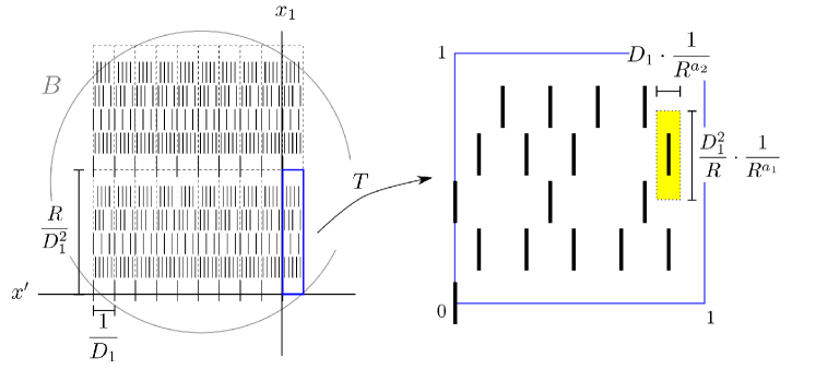
Figure 3. In blue, the unit cell $\widetilde{X}_{R}^{a_{1},a_{2}}$. On the right, $\Omega_{R}^{a_{1},a_{2}}=T(\widetilde{X}_{R}^{a_{1},a_{2}})$. In black on the right, the image by $T$ of the original slabs, and in yellow, the image of the slabs dilated by $a_{1},a_{2}$. To apply the Mass Transference Principle, we must prove that $\Omega_{k}^{\boldsymbol{a}}$ covers a positive portion of the unit cell.

Regarding $\mathcal{H}^{n}(B\cap X_{R}^{a_{1},a_{2}})$, the set $X_{k}^{a_{1},a_{2}}$ has periodic a structure, as shown in Figure 3. Indeed, under the shrinking condition

$$\frac{R}{D_{1}^{2}}\ll 1\quad\iff\quad u_{2}-u_{1}<\frac{1}{2},$$ (114)

the set $X_{k}^{a_{1},a_{2}}$ is a union of copies of the unit cell

$$\widetilde{X}_{R}^{a_{1},a_{2}}=\bigcup_{\begin{subarray}{c}Q/2\leq q\leq Q\\ q\textrm{ odd}\end{subarray}}\,\bigcup_{(p_{1},p^{\prime})\in G(q)\cap[0,q)^{n-m}}B^{1}\bigg{(}\frac{R}{D_{1}^{2}}\,\frac{p_{1}}{q},\frac{1}{R^{a_{1}}}\bigg{)}\times B^{n-m-1}\bigg{(}\frac{1}{D_{1}}\,\frac{p^{\prime}}{q},\frac{1}{R^{a_{2}}}\bigg{)},$$ (115)

which we mark in blue in Figure 3. In this situation, the number of unit cells in a ball $B^{n-m}$ is approximately $\mathcal{H}^{n}(B)D_{1}^{n-m-1}D_{1}^{2}/R$, so

$$\mathcal{H}^{n-m}(B^{n-m}\cap X_{R}^{a_{1},a_{2}})\simeq\mathcal{H}^{n-m}(B^{n-m})\,\frac{D_{1}^{n-m+1}}{R}\,\mathcal{H}^{n-m}(\widetilde{X}_{R}^{a_{1},a_{2}})$$ (116)

To compute $\mathcal{H}^{n-m}(\widetilde{X}_{R}^{a_{1},a_{2}})$, we use the transformation $T:(x_{1},x^{\prime})\mapsto(D_{1}^{2}x_{1}/R,D_{1}x^{\prime})$, which sends $\widetilde{X}_{R}^{a_{1},a_{2}}$ to the set

$$\Omega_{R}^{a_{1},a_{2}}=T\widetilde{X}_{R}^{a_{1},a_{2}}=\bigcup_{\begin{subarray}{c}Q/2\leq q\leq Q\\ q\textrm{ odd}\end{subarray}}\,\bigcup_{(p_{1},p^{\prime})\in G(q)\cap[0,q)^{n-m}}B^{1}\bigg{(}\frac{p_{1}}{q},\frac{D_{1}^{2}}{R^{1+a_{1}}}\bigg{)}\times B^{n-m-1}\bigg{(}\frac{p^{\prime}}{q},\frac{D_{1}}{R^{a_{2}}}\bigg{)}.$$ (117)

Since $\mathcal{H}^{n-m}(\widetilde{X}_{R}^{a_{1},a_{2}})=\mathcal{H}^{n-m}(\Omega_{R}^{a_{1},a_{2}})\,R/D_{1}^{n-m+1}$, then from (111), (113) and (116) we see that

$$\begin{split}\mathcal{H}^{n}(B\cap F_{R}^{\boldsymbol{a}})&\simeq\mathcal{H}^{m}(B^{m})\,\mathcal{H}^{n-m}(B^{n-m})\,\mathcal{H}^{n-m}(\Omega_{R}^{a_{1},a_{2}})\\ &\simeq\mathcal{H}^{n}(B)\,\mathcal{H}^{n-m}(\Omega_{R}^{a_{1},a_{2}}).\end{split}$$ (118)

Thus, having chosen $a_{3}=u_{3}$, to verify (103) it suffices to find $a_{1},a_{2}$ such that

$$\mathcal{H}^{n-m}(\Omega_{R}^{a_{1},a_{2}})\geq c>0,\qquad\textrm{for }R\gg 1.$$ (119)

To do so, we use a lemma from [1].

Lemma 3.4 (Lemma 4.1 of [1]).

Let $J$ be a finite set of indices and $\{I_{j}\}_{j\in J}$ be a collection of measurable sets in $\mathbb{R}^{n}$. Suppose that these sets have comparable size, that is, $B_{0}\leq\lvert I_{j}\rvert\leq B_{1}$ for all $j\in J$, and that they are regularly distributed in the sense that

$$\lvert\{(j,j^{\prime})\in J\times J\mid I_{j}\cap I_{j^{\prime}}\neq\emptyset\}\rvert\leq C\lvert J\rvert.$$ (120)

Then,

$$\Big{|}\bigcup_{j\in J}I_{j}\Big{|}\geq\frac{B_{0}}{B_{1}C}\sum_{j\in J}\lvert I_{j}\rvert.$$ (121)

With the aid of Lemma 3.4, we adapt [1, Lemma 4.2] to estimate the measure of $\Omega_{R}^{a_{1},a_{2}}$.

Lemma 3.5.

Let $Q\gg 1$, $t_{1},t_{2}\geq 1$ and $\Omega\subset\mathbb{R}^{N}$ defined as

$$\Omega=\bigcup_{\begin{subarray}{c}Q/2\leq q\leq Q\\ q\textrm{ odd}\end{subarray}}\,\bigcup_{\begin{subarray}{c}(p_{1},p^{\prime})\in[0,q)^{N}\\ \operatorname{gcd}(p_{1},q)=1\end{subarray}}B^{1}\bigg{(}\frac{p_{1}}{q},\frac{1}{Q^{t_{1}}}\bigg{)}\times B^{N-1}\bigg{(}\frac{p^{\prime}}{q},\frac{1}{Q^{t_{2}}}\bigg{)}.$$ (122)

If

$$t_{1}+(N-1)t_{2}=N+1,$$ (123)

there exists $c>0$ such that $\mathcal{H}^{N}(\Omega)\geq c>0.$

Proof.

We apply Lemma 3.4 with

$$J=\{(p_{1},p^{\prime},q)\mid Q/2\leq q\leq Q,\quad q\textrm{ odd},\quad p\in[0,q)^{N}\,\,\textrm{ and }\,\,\operatorname{gcd}(p_{1},q)=1\,\}$$ (124)

and

$$I_{p_{1},p^{\prime},q}=B^{1}\bigg{(}\frac{p_{1}}{q},\frac{1}{Q^{t_{1}}}\bigg{)}\times B^{N-1}\bigg{(}\frac{p^{\prime}}{q},\frac{1}{Q^{t_{2}}}\bigg{)}.$$ (125)

By the hypothesis (123), $\lvert I_{p_{1},p^{\prime},q}\rvert=Q^{-t_{1}-(N-1)t_{2}}=Q^{-(N+1)}$. Thus, the first hypothesis of Lemma 3.4 is satisfied with $B_{0}=B_{1}$. On the other hand, the size of the index set is

$$\lvert J\rvert=\sum_{\begin{subarray}{c}Q/2\leq q\leq Q\\ q\textrm{ odd}\end{subarray}}\varphi(q)\,q^{N-1}.$$ (126)

We use the formula $\varphi(q)=q\sum_{d\mid q}\mu(d)/d$, where $\mu$ is the Möbius function [18, Sec. 16.3], to write

$$\lvert J\rvert =\sum_{\begin{subarray}{c}Q/2\leq q\leq Q\\ q\textrm{ odd}\end{subarray}}q^{N}\,\sum_{d\,\mid\,q}\frac{\mu(d)}{d}\quad\simeq\quad Q^{N}\,\sum_{d\in\mathbb{N}}\frac{\mu(d)}{d}\sum_{\begin{subarray}{c}Q/2\leq q\leq Q\\ q\textrm{ odd}\end{subarray}}\mathds{1}_{\{d\,\mid\,q\}}$$ (127)

$$=Q^{N}\,\sum_{d\in\mathbb{N},\,d\textrm{ odd}}\frac{\mu(d)}{d}\sum_{\begin{subarray}{c}Q/(2d)\leq k\leq Q/d\\ k\textrm{ odd}\end{subarray}}1$$ (128)

If $Q$ is large enough, then

$$|J|\simeq Q^{N}\sum_{d\in\mathbb{N},\,d\textrm{ odd}}\frac{\mu(d)}{d}\,\frac{Q}{d}\quad=\quad Q^{N+1}\sum_{d\in\mathbb{N},\,d\textrm{ odd}}\frac{\mu(d)}{d^{2}}\quad\simeq\quad Q^{N+1},$$ (130)

where the last sum is finite because $\mu(d)\in\{-1,0,1\}$ for all $d\in\mathbb{N}$. Hence, to apply Lemma 3.4 we have to prove

$$\lvert\{(j,j^{\prime})\in J\times J\,\mid\,I_{j}\cap I_{j^{\prime}}\neq\emptyset\}\rvert\lesssim Q^{N+1}.$$ (131)

First, the diagonal contribution of equal indices $j=j^{\prime}$ is $\lvert J\rvert$, so it is enough to prove

$$\lvert\{(j,j^{\prime})\in J\times J\mid j\neq j^{\prime}\textrm{ and }I_{j}\cap I_{j^{\prime}}\neq\emptyset\}\rvert\lesssim Q^{N+1}.$$ (132)

To prove (132), let us first fix $q$ and $\widetilde{q}$ and count all $j=(p_{1},p^{\prime},q)$ and $j^{\prime}=(\widetilde{p}_{1},\tilde{p}^{\prime},\widetilde{q})$ such that $I_{j}\cap I_{j^{\prime}}\neq\emptyset$. In this case,

$$\Big{|}\frac{p_{1}}{q}-\frac{\widetilde{p}_{1}}{\widetilde{q}}\Big{|}<\frac{2}{Q^{t_{1}}}\qquad\mbox{and}\qquad\Big{|}\frac{p_{l}}{q}-\frac{\widetilde{p}_{l}}{\widetilde{q}}\Big{|}<\frac{2}{Q^{t_{2}}},\quad l=2,\ldots,N$$ (133)

There are two cases:

• Case $\boldsymbol{q=\widetilde{q}}$. From (133) and $t_{1},t_{2}\geq 1$ we have that $0<\lvert p_{l}-\widetilde{p}_{l}\rvert<2$ for all $l$. Thus, for each $q$, we can pick $\lesssim Q^{N}$ pairs $(j,j^{\prime})$. Summing over all odd $q$, the total contribution is of the order of $Q^{N+1}$.

• Case $\boldsymbol{q\neq\widetilde{q}}$. From (133) we have that

  $$\lvert\widetilde{q}p_{1}-q\widetilde{p}_{1}\rvert\leq 2Q^{2-t_{1}}\qquad\mbox{and}\qquad\lvert\widetilde{q}p_{l}-q\widetilde{p}_{l}\rvert\leq 2Q^{2-t_{2}},\quad l=2,\ldots,N.$$ (134)

  Let us fix $l=1,\ldots,N$ and count the number of $0\leq p_{l}<q$ and $0\leq\widetilde{p}_{l}<\widetilde{q}$ that satisfy (134). Let $d=\operatorname{gcd}(q,\widetilde{q})$ and write $q=sd$, $\widetilde{q}=\widetilde{s}d$ such that $\operatorname{gcd}(s,\widetilde{s})=1$.

  Call $m=\widetilde{q}p_{l}-q\widetilde{p}_{l}$. We want to count the number of ways we can write $m$ like that, that is, how many $0\leq r_{l}<q$ and $0\leq\widetilde{r}_{l}<\widetilde{q}$ satisfy $\widetilde{q}p_{l}-q\widetilde{p}_{l}$? We would have $\widetilde{s}p_{l}-s\widetilde{p}_{l}=\widetilde{s}r_{l}-s\widetilde{r}_{l}$, which implies $s\mid p_{l}-r_{l}$, or equivalently $0\leq r_{l}=p_{l}+ks<q$ for some $k\in\mathbb{N}$. The last inequality can hold at most for $d$ different values of $k$. Thus, we can write $m$ in at most $d$ different ways.

  On the other hand, necessarily $d\mid m$. Since $\lvert m\rvert\leq 2Q^{2-t_{i}}$, we can work with at most $2Q^{2-t_{i}}/d$ values of $m$. Since each of them can be written in $d$ different ways, we conclude that the number of pairs $p_{l}$ and $\widetilde{p}_{l}$ satisfying (134) is at most $Q^{2-t_{i}}$.

  Since $l=1$ goes with $t_{1}$ and $l=2,\ldots,N$ go with $t_{2}$, for each fixed $q$ and $\widetilde{q}$ the number of $p$ and $\widetilde{p}$ is at most $Q^{2-t_{1}}\,Q^{(2-t_{2})(N-1)}=Q^{N-1}$. Finally, summing over all different $q$ and $\widetilde{q}$ gives a total contribution of the order of $Q^{N+1}$.

The two cases together prove (132). Thus, we can use Lemma 3.4 and write

$$\mathcal{H}^{n}(\Omega) \gtrsim\sum_{\begin{subarray}{c}Q/2\leq q\leq Q\\ q\textrm{ odd}\end{subarray}}\,\sum_{\begin{subarray}{c}(p_{1},p^{\prime})\in[0,q)^{N}\\ \operatorname{gcd}(p_{1},q)=1\end{subarray}}\lvert I_{p_{1},p^{\prime},q}\rvert\quad\simeq\quad\sum_{\begin{subarray}{c}Q/2\leq q\leq Q\\ q\textrm{ odd}\end{subarray}}\frac{\varphi(q)\,q^{N-1}}{Q^{t_{1}+(N-1)t_{2}}}$$ (135)

$$\simeq\frac{1}{Q^{2}}\,\sum_{\begin{subarray}{c}Q/2\leq q\leq Q\\ q\textrm{ odd}\end{subarray}}\varphi(q)\quad\simeq\quad 1,$$ (136)

where the last equality follows proceeding like in (127). ∎

With Lemma 3.5 we get the conditions that we need for $a_{1}$ and $a_{2}$ in order to have (119).

Lemma 3.6.

For the parameters $u_{1},u_{2}$ satisfying the restrictions (85), (86) and (114), let $a_{1}$ and $a_{2}$ be such that

$$u_{1}\leq a_{1}\qquad\mbox{and}\qquad u_{2}\leq a_{2},$$ (137)

and

$$a_{1}+(n-m-1)a_{2}=(n-m+1)u_{2}-1$$ (138)

Then, there exists $c>0$ such that

$$\mathcal{H}^{n-m}(\Omega_{R}^{a_{1},a_{2}})\geq c>0,\qquad\forall R\gg 1.$$ (139)

Proof.

For $\Omega_{R}^{a_{1},a_{2}}$, which we defined in (117), we want to apply Lemma 3.5 with $N=n-m$ and

$$\frac{1}{Q^{t_{1}}}=\frac{D_{1}^{2}}{R^{1+a_{1}}}=\frac{1}{R^{a_{1}-1-2(u_{1}-u_{2})}}\qquad\mbox{and}\qquad\frac{1}{Q^{t_{2}}}=\frac{D_{1}}{R^{a_{2}}}=\frac{1}{R^{a_{2}-1-(u_{1}-u_{2})}}.$$ (140)

For that, we need $Q=R^{2u_{2}-u_{1}-1}\gg 1$, which means $2u_{2}-u_{1}-1>0$. In that case, we get

$$t_{1}=\frac{a_{1}-1-2(u_{1}-u_{2})}{2u_{2}-u_{1}-1},\qquad t_{2}=\frac{a_{2}-1-(u_{1}-u_{2})}{2u_{2}-u_{1}-1}.$$ (141)

The condition $t_{1}\geq 1$ implies $a_{1}\geq u_{1}$, while $t_{2}\geq 1$ implies $a_{2}\geq u_{2}$. On the other hand, replacing (141) in (123) we get the condition

$$a_{1}+(n-m-1)a_{2}=(n-m+1)u_{2}-1,$$ (142)

under which there exists $c>0$ such that $\mathcal{H}^{n-m}(\Omega_{R}^{a_{1},a_{2})}\geq c$.

According to restriction (86), we are only left with the case $2u_{2}-u_{1}-1=0$, which corresponds to $Q=1$. In this case, the set turns into

$$\Omega_{R}^{a_{1},a_{2}}=B^{1}\bigg{(}0,\frac{D_{1}^{2}}{R^{1+a_{1}}}\bigg{)}\times B^{n-m-1}\bigg{(}0,\frac{D_{1}}{R^{a_{2}}}\bigg{)},$$ (143)

so we get $\mathcal{H}^{n-m}(\Omega_{R}^{a_{1},a_{2})}\geq c>0$ if we ask $D_{1}^{2}=R^{1+a_{1}}$ and $D_{1}=R^{a_{2}}$. This amounts to $a_{1}=u_{1}$ and $a_{2}=u_{2}$. Observe that (138) is also satisfied in this case. ∎

Remark 3.7.

The restrictions we found for the parameters $(u_{1},u_{2},u_{3})$ and the dilation exponents $(a_{1},a_{2},a_{3})$ are the following:

For the parameters, from (85), (86) and (114) we have

$$0<u_{1},u_{3}\leq 1/2,\qquad 0<u_{2}\leq 1,\qquad 2u_{2}-u_{1}\geq 1,\qquad u_{2}-u_{1}<1/2.$$ (144)

In particular, $u_{2}>1/2$. Regarding $(a_{1},a_{2},a_{3})$, we got

$$u_{1}\leq a_{1}\leq 1/2,\qquad u_{2}\leq a_{2}\leq 1,\qquad a_{3}=u_{3},\qquad a_{1}+(n-m-1)a_{2}=(n-m+1)u_{2}-1.$$ (145)

From the last restriction in (145) together with $a_{1}\leq 1/2$ and $a_{2}\leq 1$ we get the additional restriction

$$(n-m+1)u_{2}\leq n-m+1/2.$$ (146)

Thus, for $(u_{1},u_{2},u_{3})$ that satisfy (144) and (146), we can always find $(a_{1},a_{2},a_{3})$ that satisfy (145), so (119) holds and we can use the Mass Transference Principle.

The restrictions for $(u_{1},u_{2},u_{3})$ are shown in Figure 4.

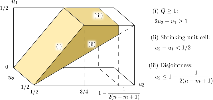
Figure 4. Restrictions on $\boldsymbol{u}=(u_{1},u_{2},u_{3})$.

According to Remark 3.7 we can apply the Mass Transference Principle in Theorem 3.2. With it, we show that the upper bound given in Proposition 3.1 is sharp.

Proposition 3.8.

Let $F\subset\mathbb{R}^{n}$ be the divergence set defined in (61) and (63), with parameters $(u_{1},u_{2},u_{3})$ as in Remark 3.7. Then,

$$\operatorname{dim_{\mathcal{H}}}F=\min\{\alpha_{1},\alpha_{2}\},$$ (147)

where

$$\alpha_{1}=\alpha_{1}(u_{2},u_{3})=\frac{m-1}{2}+(n-m+1)u_{2}+mu_{3}$$ (148)

and

$$\alpha_{2}=\alpha_{2}(u_{2},u_{3})=\begin{cases}n-m-3+4u_{2}+2mu_{3},&\mbox{for}\quad u_{2}\leq 3/4\\ n-m+2mu_{3},&\mbox{for}\quad u_{2}\geq 3/4.\end{cases}$$ (149)

Proof.

By Lemma 3.1, we only have to prove the lower bound.

For any $(u_{1},u_{2},u_{3})$ as in Remark 3.7, we can find $(a_{1},a_{2},a_{3})$ that satisfy (145). Then, Lemma 3.6 proves (119), which allows us to use the Mass Transference Principle in Theorem 3.2. Since $\boldsymbol{b}=(1/2,1,1/2)$, then

$$\operatorname{dim_{\mathcal{H}}}F\geq\min_{B\in\{1,1/2\}}\bigg{\{}\sum_{j\in K_{1}(B)}1+\sum_{j\in K_{2}(B)}\Big{(}1-\frac{b_{j}-a_{j}}{B}\Big{)}+\sum_{j\in K_{3}(B)}\frac{a_{j}}{B}\bigg{\}},$$ (150)

where

$$\begin{array}[]{c}K_{1}(B)=\{j\mid a_{j}\geq B\},\qquad\qquad K_{2}(B)=\{j\mid b_{j}\leq B\}\setminus K_{1}(B),\\ \\ K_{3}(B)=\{1,\ldots,n\}\setminus(K_{1}(B)\cap K_{2}(B)).\end{array}$$ (151)

We compute each term in the minimum (150) separately:

• $B=1$: If $a_{2}<1$, we get $K_{1}(1)=\emptyset$, $K_{2}(1)=\{1,\ldots,n\}$ and $K_{3}(1)=\emptyset$, so the term in braces is

  $$n-\sum_{j=1}^{n}b_{j}+\sum_{j=1}^{n}a_{j}\\ =\frac{m+1}{2}+a_{1}+(n-m-1)a_{2}+ma_{3}.$$ (152)

  Replacing (145) above, we get

  $$\alpha_{1}=\alpha_{1}(u_{2},u_{3})=\frac{m-1}{2}+(n-m+1)u_{2}+mu_{3}.$$ (153)

  If $a_{2}=1$, then $K_{1}(1)=\{2,\ldots,n-m\}$, $K_{2}(1)=\{1,n-m+1,\ldots,n\}$ and $K_{3}(1)=\emptyset$. Thus, we get

  $$(n-m-1)+(m+1)-(1/2-a_{1})-m(1/2-a_{3})=n-\frac{m+1}{2}+a_{1}+ma_{3},$$ (154)

  This is equal to (152), so we get the same $\alpha_{1}$.

• $B=1/2$: Let us first assume that $a_{1},a_{3}<1/2$ so that $K_{1}(1/2)=\{2,\ldots,n-m\}$, $K_{2}(1/2)=\{1,n-m+1,\ldots,n\}$ and $K_{3}(1/2)=\emptyset$. The term in braces is thus

  $$\alpha_{2}(u_{3},a_{1}) =(n-m-1)+(m+1)-(1-2a_{1})-m(1-2a_{3})$$ (155)

  $$=n-m-1+2a_{1}+2mu_{3}.$$ (156)

  In the case that $a_{1}<1/2$ and that $a_{3}=1/2$, we have $K_{1}(1/2)=\{2,\ldots,n\}$, $K_{2}(1/2)=\{1\}$ and $K_{3}(1/2)=\emptyset$, and we get

  $$\alpha_{2}(a_{1}) =(n-1)+1-(1-2a_{1})=n-1+2a_{1},$$ (157)

  which is the same as (156) because $u_{3}=a_{3}=1/2$. Similarly, the cases $a_{1}=1/2$, $a_{3}<1/2$ and $a_{1}=a_{3}=1/2$ yield the same result.

Joining the two expressions for the minimum, we get

$$\operatorname{dim_{\mathcal{H}}}F\geq\min\{\alpha_{1}(u_{2},u_{3}),\alpha_{2}(u_{3},a_{1})\},\qquad\forall a_{1}\text{ like in }\eqref{eq:Restrictions_Dilation}.$$ (158)

Thus, we want to choose the value of $a_{1}$ that gives the largest $\alpha_{2}(u_{3},a_{1})$.

According to (156), we need to take the largest possible $a_{1}$. Since $a_{1}\leq 1/2$, in principle we may take $a_{1}=1/2$. In view of (145), that implies

$$(n-m+1)u_{2}=3/2+(n-m-1)a_{2}.$$ (159)

However, we need $a_{2}\geq u_{2}$, which under the restriction (159) is equivalent to $u_{2}\geq 3/4$. Thus, we separate two cases:

• If $u_{2}\leq 3/4$, then $a_{1}=1/2$ is admissible, so the maximum for $\alpha(u_{3},a_{1})$ is

  $$\alpha_{2}(u_{3})=n-m+2mu_{3},\qquad\text{ if }u_{2}\geq 3/4.$$ (160)

• If $u_{2}<3/4$, then $a_{1}=1/2$ is not admissible, because $a_{2}<u_{2}$. Then, the largest admissible value for $a_{1}$ corresponds to $a_{2}=u_{2}$, which in view of (145) gives $a_{1}=2u_{2}-1$. Thus, the maximum $\alpha_{2}$ is

  $$\alpha_{2}(u_{2},u_{3})=n-m-3+4u_{2}+2mu_{3},\qquad\text{ if }u_{2}<3/4.$$ (161)

Consequently, from (158), we obtain

$$\operatorname{dim_{\mathcal{H}}}F\geq\min\{\alpha_{1}(u_{2},u_{3}),\alpha_{2}(u_{2},u_{3})\},$$ (162)

where $\alpha_{1}$ is defined in (153) and $\alpha_{2}$ is defined in (160) and (161). The proof is complete. ∎

3.3. The case $\boldsymbol{m=n-1}$

The counterexample is not as interesting in this case because the Talbot effect is absent. We discuss it briefly. The set of divergence is actually much simpler, given by

$$F=\limsup_{k\to\infty}F_{k}=\limsup_{k\to\infty}\bigcup_{p\in\mathbb{Z}^{m}}E_{k}(p)$$ (163)

$$E_{k}(p)=[-1,0]\times B^{n-1}\bigg{(}\frac{p}{D_{2,k}},R_{k}^{-1/2}\bigg{)},$$ (164)

so only the parameter $D_{2}=R^{u_{3}}$ survives. We use the Mass Transference Principle Theorem 3.2 in $\mathbb{R}^{n-1}$ with $\boldsymbol{a}=(a,\ldots,a)$, which corresponds to the original version in [3]. The dilation $a$ needed for the local ubiquity condition (103) must satisfy $D_{2}=R^{\frac{a}{2(n-1)}}$, that is, $a=2(n-1)u_{3}$, which implies $\operatorname{dim_{\mathcal{H}}}F=1+2(n-1)u_{3}$. The dimension can also be computed using the methods in Section 8.2 of [17].

4. Sobolev Regularity

We begin by recalling that the Sobolev regularity $s_{m}=s_{m}(Q,D_{1},D_{2})$ of the counterexample was given in (57) by

$$R^{s_{m}}=R^{1/4}\,\left(\frac{R}{D_{1}Q}\right)^{(n-m-1)/2}\,\left(\frac{R^{1/2}}{D_{2}}\right)^{m/2}.$$ (165)

Using (82), we rewrite it in terms of the geometric parameters $(u_{1},u_{2},u_{3})$ as

$$s_{m}(u_{2},u_{3})=\frac{2n-m-1}{4}-\frac{n-m-1}{2}u_{2}-\frac{mu_{3}}{2}.$$ (166)

Given a fixed dimension $\alpha$, we want to maximize $s_{m}$. As we showed in Proposition 3.8, the dimension of the divergence set is a function $\alpha(u_{2},u_{3})$, so we are imposing the restriction $\alpha=\alpha(u_{2},u_{3})$. This still leaves one degree of freedom $v$ in $s_{m}(\alpha,v)$, which we might set either as $u_{2}$ or as $u_{3}$. Let us denote the maximum regularity by $s_{m}(\alpha)=\max_{v}s_{m}(\alpha,v)$.

The case $m=0$ corresponds to the counterexample studied in [22], which gives the regularity

$$s_{m}(\alpha)=\frac{n}{2(n+1)}+\frac{n-1}{2(n+1)}(n-\alpha),$$ (167)

so we focus on $m\geq 1$. Fix $\operatorname{dim_{\mathcal{H}}}F=\alpha$. By Proposition 3.8,

$$\alpha=\min\{\alpha_{1}(u_{2},u_{3}),\alpha_{2}(u_{2},u_{3})\},$$ (168)

where

$$\alpha_{1}=\frac{m-1}{2}+(n-m+1)u_{2}+mu_{3}\quad\mbox{and}\quad\alpha_{2}=\begin{cases}n-m-3+4u_{2}+2mu_{3},&\mbox{for }u_{2}\leq 3/4\\ n-m+2mu_{3},&\mbox{for }u_{2}\geq 3/4.\end{cases}$$ (169)

This is a restriction on $(u_{2},u_{3})$, which takes the form of a broken line in the $(u_{2},u_{3})$ plane. We want to pick a point $(u_{2},u_{3})$ that gives the maximum $s_{m}(u_{2},u_{3})$. In the arguments that follow, we suggest the reader to use Figures 5, 6 and 7 as visual support.

According to the restrictions in Remark 3.7, we have

$$(u_{2},u_{3})\in\mathcal{D}=\left[\,\frac{1}{2},\,1-\frac{1}{2(n-m+1)}\right]\times\left[0,1/2\right].$$ (170)

Let us first determine in $\mathcal{D}$ the boundary between the two lines in (168). If $u_{2}\geq 3/4$,

$$\alpha_{1}\leq\alpha_{2}\quad\Longleftrightarrow\quad(n-m+1)u_{2}-mu_{3}\leq n-\frac{3m}{2}+\frac{1}{2},$$ (171)

so the boundary is

$$(n-m+1)u_{2}-mu_{3}=n-\frac{3m}{2}+\frac{1}{2},\qquad\text{ when }u_{2}\geq 3/4.$$ (172)

This line crosses the points

$$(u_{2},u_{3})=\left(1-\frac{1}{2(n-m+1)},\,\frac{1}{2}\right)\quad\text{ and }\quad(u_{2},u_{3})=\left(1-\frac{m+1}{2(n-m+1)},\,0\right),$$ (173)

so it is completely in $\mathcal{D}\cap\{u_{2}\geq 3/4\}$ if

$$1-\frac{1}{2(n-m+1)}\geq\frac{3}{4}\quad\Longleftrightarrow\quad m\leq\frac{n-1}{3}.$$ (174)

This shows that we need to separate cases for $m$, and it will become evident that we also need to study the cases $n-3\leq m\leq n-1$ separately.

4.1. When $\boldsymbol{m<n-3}$ and $\boldsymbol{m\leq(n-1)/3}$

This case is displayed in Figure 5. According to (174), the boundary line (172) is completely included in $u_{2}\geq 3/4$. This suggests that in $u_{2}\leq 3/4$ we always have $\alpha_{1}\leq\alpha_{2}$. Indeed,

$$\begin{split}\alpha_{1}\leq\alpha_{2}\,&\Longleftrightarrow\,\frac{m-1}{2}+(n-m+1)\,u_{2}+mu_{3}\leq n-m-3+4u_{2}+2mu_{3}\\ &\Longleftrightarrow(n-m-3)\,u_{2}-mu_{3}\leq n-\frac{3m}{2}-\frac{5}{2},\end{split}$$ (175)

and together with $u_{2}\leq 3/4$ and $u_{3}\geq 0$, the condition $m\leq(n-1)/3$ allows us to write

$$(n-m-3)\,u_{2}-mu_{3}\leq\frac{3}{4}\,(n-m-3)\leq n-\frac{3m}{2}-\frac{5}{2}.$$ (176)

Thus, when $u_{2}\leq 3/4$ we have $\min\{\alpha_{1},\alpha_{2}\}=\alpha_{1}$.

Let us compute the Sobolev regularity:

• In the region where $\min\{\alpha_{1},\alpha_{2}\}=\alpha_{2}$, since $u_{2}\geq 3/4$, we may write

  $$\alpha=n-m+2mu_{3}\quad\Longrightarrow\quad mu_{3}=\frac{m-(n-\alpha)}{2}.$$ (177)

  Consequently, $u_{3}$ is fixed. Replacing in (166), we get

  $$s_{m}(\alpha,u_{2})=\frac{n-\alpha+1}{4}+\frac{n-m-1}{2}(1-u_{2}).$$ (178)

  Thus, to maximize $s_{m}(\alpha,u_{2})$ we need to minimize $u_{2}$. This is attained on the boundary (172).

• In the region where $\min\{\alpha_{1},\alpha_{2}\}=\alpha_{1}$ we have

  $$\alpha=\frac{m-1}{2}+(n-m+1)u_{2}+mu_{3},$$ (179)

  so replacing in (166) we get

  $$s_{m}(\alpha,u_{2})=\frac{n-1-\alpha}{2}+u_{2}.$$ (180)

  In this case, to maximize $s_{m}(\alpha,u_{2})$ we need to maximize $u_{2}$. The maximum $u_{2}$ in this region may be either on the boundary (172) or in $u_{3}=0$.

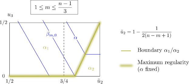
Figure 5. For fixed $\alpha$, the maximum regularity is attained on the blurred, green line.

Thus, in all cases, given a dimension $\alpha$, the maximum $s_{m}(\alpha)=\max_{u_{2}}s_{m}(\alpha,u_{2})$ is attained either on the boundary (172) or on $u_{3}=0$. Let $\beta_{m,0}$ be the dimension where this transition happens, that is, the value $\beta_{m,0}$ such that the line $\beta_{m,0}=\min\{\alpha_{1},\alpha_{2}\}$ crosses the intersection of the boundary (172) and $u_{3}=0$. When $\beta_{m,0}=\alpha_{2}$, we are always in $u_{2}\geq 3/4$, so we may write $\beta_{m,0}=\alpha_{2}=n-m+2mu_{3}$. Since the point of intersection has $u_{3}=0$, we deduce that

$$\beta_{m,0}=n-m.$$ (181)

This generates two different cases for $\alpha$:

• If $\alpha\leq\beta_{m,0}$, then $\alpha=\min\{\alpha_{1},\alpha_{2}\}=\alpha_{1}(u_{2},u_{3})$ and the maximum $s_{m}(\alpha)$ is attained at $u_{3}=0$. Thus, from (179) and (180),

  $$s_{m}(\alpha)=\frac{n}{2(n-m+1)}+\frac{n-m-1}{2(n-m+1)}(n-\alpha),\qquad\text{ if }\quad n/2\leq\alpha\leq n-m.$$ (182)

  Observe that the smallest possible $\alpha$ corresponds to $\alpha=\alpha_{1}(u_{2},u_{3})$ crossing the point $(u_{2},u_{3})=(1/2,0)$, which gives $\alpha_{\text{min}}=n/2$.

• If $\beta_{m,0}\leq\alpha\leq n$, the maximum of $s_{m}(\alpha,u_{2})$ is attained on the boundary (172). The intersection between the broken line $\alpha=\min\{\alpha_{1},\alpha_{2}\}$ and the boundary (172) is determined by

  $$(n-m+1)u_{2}=n-m-\frac{n-\alpha-1}{2}\qquad\text{and}\qquad 2mu_{3}=m-(n-\alpha).$$ (183)

  Replacing this point either in (178) or in (180), we get

  $$s_{m}(\alpha)=\frac{n-m}{2(n-m+1)}+\frac{n-m}{2(n-m+1)}(n-\alpha),\qquad\text{ if }\quad n-m\leq\alpha\leq n.$$ (184)

4.2. When $\boldsymbol{m<n-3}$ and $\boldsymbol{(n-1)/3<m\leq n/2-1}$

We display this case at the left of Figure 6. Now the boundary (172) crosses $u_{2}\geq 3/4$ while in $\mathcal{D}$, and the crossing point is

$$(u_{2},u_{3})=\Big{(}\frac{3}{4},\,\frac{1}{2}-\frac{n-m-1}{4m}\Big{)}.$$ (185)

In this case, $\min\{\alpha_{1},\alpha_{2}\}$ also changes in $u_{2}\leq 3/4$ and the boundary is given by

$$\alpha_{1}=\alpha_{2}\quad\Longleftrightarrow\quad(n-m-3)u_{2}-mu_{3}=n-\frac{3m}{2}-\frac{5}{2}.$$ (186)

This line has positive slope as long as $m<n-3$, and it passes through the points (185) and

$$(u_{2},u_{3})=\Big{(}1-\frac{m-1}{2\,(n-m-3)},\,0\Big{)}.$$ (187)

It makes a difference whether the point (187) is in $\mathcal{D}$ or not. One immediately sees that

$$\eqref{eq:Point_Of_Boundary_Line_2}\in\mathcal{D}\quad\Longleftrightarrow\quad 1-\frac{m-1}{2\,(n-m-3)}\geq\frac{1}{2}\quad\Longleftrightarrow\quad m\leq\frac{n}{2}-1,$$ (188)

which is the case we are considering now.

Remark 4.1.

We saw in Subsection 4.1 that:

• When $\min\{\alpha_{1},\alpha_{2}\}=\alpha_{1}$ we need to maximize $u_{2}$.

• When $\min\{\alpha_{1},\alpha_{2}\}=\alpha_{2}$ and $u_{2}\geq 3/4$ we need to minimize $u_{2}$.

Now we have an additional case:

• When $\min\{\alpha_{1},\alpha_{2}\}=\alpha_{2}$ and $u_{2}\leq 3/4$ we have $\alpha=n-m-3+4u_{2}+2mu_{3}$, so replacing in (166) we get

  $$s_{m}(\alpha,u_{2})=\frac{n-m-2}{2}+\frac{n-\alpha}{4}-\frac{n-m-3}{2}\,u_{2}.$$ (189)

  Since $m<n-3$, to maximize $s_{m}(\alpha,u_{2})$ we need to minimize $u_{2}$.

Consequently, depending on the value of $\alpha$, the maximum of $s_{m}(\alpha,u_{2})$ is attained in the boundary (172), in the boundary (186) or in $u_{3}=0$. Let us determine which $\alpha$ corresponds to each case.

• The interval corresponding to the boundary line (172) is $\alpha\in[\beta_{m,2},n]$, where $\beta_{m,2}$ is such that the broken line $\beta_{m,2}=\min\{\alpha_{1},\alpha_{2}\}$ crosses the point (185). Thus,

  $$\beta_{m,2}=n-m+2m\left(\frac{1}{2}-\frac{n-m-1}{4m}\right)=\frac{n+m+1}{2}$$ (190)

  The analysis in this case is identical to that in (184), so

  $$s_{m}(\alpha)=\frac{n-m}{2(n-m+1)}+\frac{n-m}{2(n-m+1)}(n-\alpha),\qquad\beta_{m,2}\leq\alpha\leq n.$$ (191)

• The interval corresponding to the boundary (186), which is in $u_{2}\leq 3/4$, is $\alpha\in[\beta_{m,1},\beta_{m,2}]$, where the broken line $\beta_{m,1}=\min\{\alpha_{1},\alpha_{2}\}$ crosses the point (187). This means that

  $$\beta_{m,1}=n-m-3+4\left(1-\frac{m-1}{2(n-m-3)}\right)=n-(m-1)\,\frac{n-m-1}{n-m-3}.$$ (192)

  For $\alpha\in[\beta_{m,1},\beta_{m,2}]$, the point $(u_{2},u_{3})$ of the broken line $\alpha=\min\{\alpha_{1},\alpha_{2}\}$ that is in the boundary line (186) has

  $$u_{2}=\frac{n+\alpha-2(m+1)}{2(n-m-1)}.$$ (193)

  Thus, the Sobolev regularity we get from (189) is

  $$s_{m}(\alpha)=\frac{1}{2}+\frac{n-m-2}{2(n-m-1)}(n-\alpha),\qquad\beta_{m,1}\leq\alpha\leq\beta_{m,2}.$$ (194)

• For the last interval $\alpha\in[\alpha_{\text{min}},\beta_{m,1}]$ we have $\alpha=\alpha_{1}(u_{2},u_{3})$, and the maximum $u_{2}$ is attained at $u_{3}=0$. The procedure is the same as in (182), so we get

  $$s_{m}(\alpha)=\frac{n}{2(n-m+1)}+\frac{n-m-1}{2(n-m+1)}(n-\alpha),\qquad n/2\leq\alpha\leq\beta_{m,1}.$$ (195)

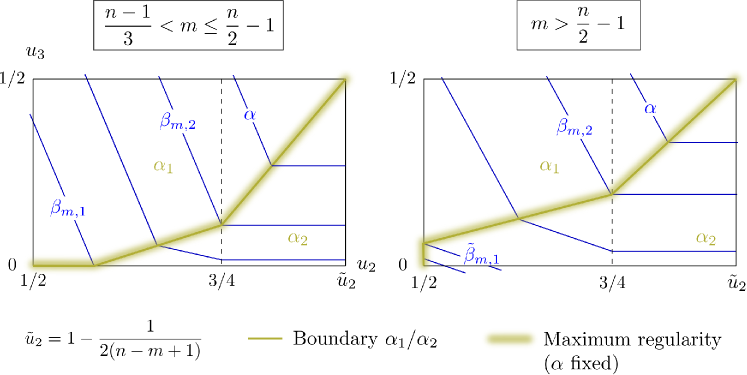
Figure 6. For fixed $\alpha$, the maximum regularity is attained on the blurred, green line.

4.3. When $\boldsymbol{n/2-1<m<n-3}$

This case is shown at the right of Figure 6. By (188), we have that (187) $\notin\mathcal{D}$. The useful point in this case is the intersection of the boundary (186) with $u_{2}=1/2$, that is,

$$u_{2}=\frac{1}{2}\qquad\mbox{and}\qquad u_{3}=\frac{m+1-n/2}{m}>0.$$ (196)

In this case, depending on $\alpha$ and again following Remark 4.1, the maximum $s_{m}(u_{2},u_{3})$ is found in the boundary (172), in the boundary (186) or on the line $u_{2}=1/2$. Let us determine the ranges for $\alpha$ in each case:

• For the interval corresponding to the boundary (172), the analysis is exactly the same as in the previous case, so we get

  $$s_{m}(\alpha)=\frac{n-m}{2(n-m+1)}+\frac{n-m}{2(n-m+1)}(n-\alpha),\qquad\beta_{m,2}\leq\alpha\leq n.$$ (197)

• The interval corresponding to the boundary (186) is $\alpha\in[\widetilde{\beta}_{m,1},\beta_{m,2}]$, where $\widetilde{\beta}_{m,1}=\min\{\alpha_{1},\alpha_{2}\}$ crosses the point (196). Evaluating in $\alpha_{1}$, we get

  $$\widetilde{\beta}_{m,1}=\frac{m-1}{2}+\frac{n-m+1}{2}+m+1-\frac{n}{2}=m+1.$$ (198)

  For $\alpha\in[\widetilde{\beta}_{m,1},\beta_{m,2}]$, the analysis is the same as in (194), so we get

  $$s_{m}(\alpha)=\frac{1}{2}+\frac{n-m-2}{2(n-m-1)}(n-\alpha),\qquad\widetilde{\beta}_{m,1}\leq\alpha\leq\beta_{m,2}.$$ (199)

• The last interval is $\alpha\in[\alpha_{\text{min}},\widetilde{\beta}_{m,1}]$, where the maximum is attained in $u_{2}=1/2$. In this case, $\alpha_{\text{min}}$ is such that $\alpha_{\text{min}}=\min\{\alpha_{1},\alpha_{2}\}$ crosses the point $(u_{2},u_{3})=(1/2,0)$, that is,

  $$\alpha_{\text{min}}=n-m-1.$$ (200)

  Thus, for $\alpha\in[\alpha_{\text{min}},\widetilde{\beta}_{m,1}]$ we have $\alpha=\alpha_{2}(u_{2},u_{3})$, so replacing $u_{2}=1/2$ in (189) we get

  $$s_{m}(\alpha)=\frac{n-m-1}{4}+\frac{n-\alpha}{4},\qquad n-m-1\leq\alpha\leq\widetilde{\beta}_{m,1}.$$ (201)

4.4. When $\boldsymbol{m=n-3}$

As shown in Figure 7, the boundary (186) is now the horizontal line

$$mu_{3}=-n+\frac{3m}{2}+\frac{5}{2}.$$ (202)

• The first interval $\alpha\in[\beta_{m,2},n]$ does not change with respect to the previous cases:

  $$s_{m}(\alpha)=\frac{n-m}{2(n-m+1)}+\frac{n-m}{2(n-m+1)}(n-\alpha),\qquad\beta_{m,2}\leq\alpha\leq n.$$ (203)

• The rest $\alpha<\beta_{m,2}$ are unified in this case. This is because when $u_{2}\leq 3/4$ we have $\alpha_{2}(u_{2},u_{3})=n-m-3+4u_{2}+2mu_{3}=4u_{2}+2mu_{3}$. Thus, for $(u_{2},u_{3})$ such that $\alpha=\alpha_{2}(u_{2},u_{3})$, the regularity is

  $$s_{m}(u_{2},u_{3})=\frac{2n-m-1}{4}-\frac{mu_{3}}{2}-\frac{n-m-1}{2}u_{2}=\frac{2n-m-1-\alpha}{4},$$ (204)

  which is independent of $u_{2}$ and $u_{3}$. That means that when $\alpha=\alpha_{2}(u_{2},u_{3})$ and $u_{2}\leq 3/4$, all $u_{2}$ give the same $s_{m}$. In particular, $s_{m}(u_{2},u_{3})$ is the same both in the boundary (202) and in $u_{2}=1/2$, so

  $$s_{m}(\alpha)=\frac{1}{2}+\frac{n-\alpha}{4},\qquad 2\leq\alpha\leq\beta_{m-2}=n-1.$$ (205)

  As in the previous case, $\alpha_{\text{min}}=n-m-1=2$.

Observe that this case matches the result of the case $n/2-1\leq m<m-3$.

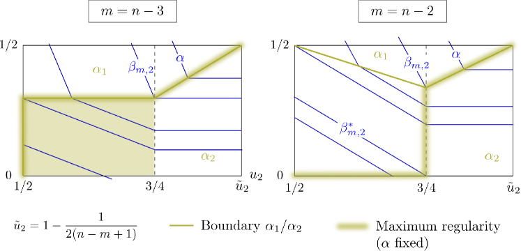
Figure 7. For fixed $\alpha$, the maximum regularity is attained on the blurred, green zone.

4.5. When $\boldsymbol{m=n-2}$

This case corresponds to the right of Figure 7. Now the boundary (186) in $u_{2}\leq 3/4$ takes the form

$$u_{2}+(n-2)u_{3}=\frac{n-1}{2}.$$ (206)

It crosses the point $(u_{2},u_{3})=(1/2,1/2)$, and its slope is $-1/(n-2)$. Observe that the slope of $\alpha=\alpha_{1}(u_{2},u_{3})$ is $-3/(n-2)$, while that of $\alpha=\alpha_{2}(u_{2},u_{3})$ in $u_{2}\leq 3/4$ is $-2/(n-2)$.

When $\alpha=\alpha_{1}(u_{2},u_{3})$ we still have (180), so we want to maximize $u_{2}$. However, when $\alpha=\alpha_{2}(u_{2},u_{3})$ and $u_{2}\leq 3/4$, the regularity we computed in (189) takes the form

$$s_{m}(\alpha)=\frac{n-\alpha}{4}+\frac{u_{2}}{2},$$ (207)

so we want to maximize $u_{2}$. When $\alpha=\alpha_{2}(u_{2},u_{3})$ and $u_{2}\geq 3/4$ the regularity is (178), so we still want to minimize $u_{2}$. Thus, depending on $\alpha$, the maximum of $s_{m}(u_{2},u_{3})$ is attained on the boundary (172) in $u_{2}\geq 3/4$, on the line $u_{2}=3/4$ or on the line $u_{3}=0$. We classify $\alpha$ accordingly:

• As in all previous cases, in the interval $\alpha\in[\beta_{m,2},n]$ the result is

  $$s_{n-2}(\alpha)=\frac{1}{3}+\frac{n-\alpha}{3},\qquad n-\frac{1}{2}\leq\alpha\leq n.$$ (208)

• The second interval is now $\alpha\in[\beta^{*}_{m,1},\beta_{m,2}]$, where $\beta^{*}_{m,1}$ corresponds to the point $(u_{2},u_{3})=(3/4,0)$, that is,

  $$\beta^{*}_{m,1}=n-m+2mu_{3}=2.$$ (209)

  In this case, the maximum is on $u_{2}=3/4$, so from (207) we get

  $$s_{n-2}(\alpha)=\frac{3}{8}+\frac{n-\alpha}{4},\qquad 2\leq\alpha\leq\beta_{m,2}=n-1/2.$$ (210)

• The last interval is $\alpha\in[\alpha_{\text{min}},\beta^{*}_{m,1}]$, and as in the previous cases $\alpha_{\text{min}}=n-m-1=1$. Now, the maximum is attained at $u_{3}=0$, and thus, $\alpha=\alpha_{2}(u_{2},u_{3})=4u_{2}-1$. Replacing this in (207) we get

  $$s_{n-2}(\alpha)=\frac{n+1}{8}+\frac{n-\alpha}{8},\qquad 1\leq\alpha\leq 2.$$ (211)

4.6. When $\boldsymbol{m=n-1}$

From (166), we have

$$s_{n-1}(u_{3})=\frac{n}{4}-\frac{n-1}{2}\,u_{3}.$$ (212)

From the dimension in Subsection 3.3, we have $\alpha=1+2(n-1)u_{3}$, where we can pick any $0<u_{3}\leq 1/2$. Thus, the regularity is

$$s_{n-1}(\alpha)=\frac{1+n-\alpha}{4},\qquad 1\leq\alpha\leq n.$$ (213)

4.7. Summary of the results of this subsection

Let us gather the results we got by defining

$$s_{3,m}(\alpha)=\frac{n}{2(n-m+1)}+\frac{n-m-1}{2(n-m+1)}(n-\alpha),$$ (214)

$$s_{4,m}(\alpha)=\frac{n-m}{2(n-m+1)}+\frac{n-m}{2(n-m+1)}(n-\alpha),$$ (215)

$$s_{5,m}(\alpha)=\frac{1}{2}+\frac{n-m-2}{2(n-m-1)}(n-\alpha),$$ (216)

and also, from (192) and (190),

$$\beta_{m,1}=n-(m-1)\,\frac{n-m-1}{n-m-3}\qquad\text{and}\qquad\beta_{m,2}=\frac{n+m+1}{2}.$$ (217)

Proposition 4.2.

Let $0\leq m\leq n-1$ and $s_{m}(\alpha)$ as below. Then, for every $s<s_{m}(\alpha)$, there exists $f\in H^{s}(\mathbb{R}^{n})$ such that $e^{it\Delta}f$ diverges in a set of dimension $\alpha$.

The exponent $s_{m}(\alpha)$ is as follows. For $0\leq m\leq n-3$:

1. If $0\leq m\leq(n-1)/3$,

   $$s_{m}(\alpha)=\begin{cases}s_{3,m}(\alpha),&\qquad n/2\leq\alpha\leq n-m,\\ s_{4,m}(\alpha),&\qquad n-m\leq\alpha\leq n.\end{cases}$$ (218)

2. If $(n-1)/3<m\leq n/2-1$,

   $$s_{m}(\alpha)=\begin{cases}s_{3,m}(\alpha),&\qquad n/2\leq\alpha\leq\beta_{m,1},\\ s_{5,m}(\alpha),&\qquad\beta_{m,1}\leq\alpha\leq\beta_{m,2},\\ s_{4,m}(\alpha),&\qquad\beta_{m,2}\leq\alpha\leq n.\end{cases}$$ (219)

3. If $n/2-1<m\leq n-3$,

   $$s_{m}(\alpha)=\begin{cases}s_{3,m}(\alpha),&\qquad n-m-1\leq\alpha\leq m+1,\\ s_{5,m}(\alpha),&\qquad m+1\leq\alpha\leq\beta_{m,2},\\ s_{4,m}(\alpha),&\qquad\beta_{m,2}\leq\alpha\leq n.\end{cases}$$ (220)

On the other hand, if $m=n-2$, then

$$s_{n-2}(\alpha)=\begin{cases}\dfrac{n+1}{8}+\dfrac{n-\alpha}{8},&\qquad 1\leq\alpha\leq 2,\\[6.0pt] \dfrac{3}{8}+\dfrac{n-\alpha}{4},&\qquad 2\leq\alpha\leq n-1/2,\\[6.0pt] \dfrac{1}{3}+\dfrac{n-\alpha}{3},&\qquad n-1/2\leq\alpha\leq n,\end{cases}$$ (221)

and if $m=n-1$, then

$$s_{n-1}(\alpha)=\frac{1+n-\alpha}{4},\qquad 1\leq\alpha\leq n.$$ (222)

The reader may want to compare the first two cases in Proposition 4.2 with Lemma 3.2 in [11]; in Du’s paper replace $d$ by $n+1$, $m$ by $m+1$, and $\kappa_{i}$ by $s_{i,m}$.

5. Maximum Regularity

For each $0\leq m\leq n-1$, Proposition 4.2 gives the regularity $s_{m}(\alpha)$ for the counterexample. Thus, we immediately get the following theorem.

Theorem 5.1.

Let $n/2\leq\alpha\leq n$. For every $0\leq m\leq n-1$, and for $s_{m}(\alpha)$ as in Proposition 4.2, define

$$s(\alpha)=\max_{0\leq m\leq n-1}s_{m}(\alpha).$$ (223)

Then, for $s<s(\alpha)$ there exists $f\in H^{s}(\mathbb{R}^{n})$ such that $e^{it\Delta}f$ diverges in a set of dimension $\alpha$.

Our aim in this section is to dissect this quantity. First, we show that in the maximum (223) it suffices to consider small $m$.

Lemma 5.2.

Let $m_{1}=\lfloor n/2-1\rfloor$. Then,

$$s(\alpha)=\max_{0\leq m\leq m_{1}}s_{m}(\alpha)$$ (224)

In particular,

$$s(\alpha)=s_{0}(\alpha),\qquad\text{ when }n=2,3.$$ (225)

Proof.

The objective is to discard the contribution of every $m>m_{1}$ to the maximum. For that, we are going to prove that $s_{m}(\alpha)\leq s_{0}(\alpha)$ for $n/2\leq\alpha\leq n$.

First observe that for $\alpha=n$, $s_{m}(n)\leq s_{0}(n)$ holds for all $m$. Thus, we may work with $\alpha<n$. We now study each $m$ separately.

• For $m=n-1$, from Proposition 4.2 we have $s_{n-1}(\alpha)=(1+n-\alpha)/4$ for every $1\leq\alpha\leq n$. Since $s_{n-1}(n/2)\leq s_{0}(n/2)=n/4$ and $s_{n-1}(n)\leq s_{0}(n)$, we deduce $s_{n-1}(\alpha)\leq s_{0}(\alpha)$ for all $\alpha$, so we may discard $s_{n-1}$.

In particular, when $n=2$ we get $s(\alpha)=s_{0}(\alpha)$. Thus, we continue with $n\geq 3$.

• If $m=n-2$, it suffices to show that $s_{n-2}(\alpha)\leq s_{0}(\alpha)$ for $\alpha=n/2$ and $n-1/2$. When $n\geq 4$ we have

  $$s_{n-2}(n/2)=\frac{n+3}{8}\leq\frac{n}{4}=s_{0}(n/2)\quad\iff\quad 3\leq n,$$ (226)

  $$s_{n-2}(n-1/2)=\frac{1}{2}\leq\frac{3n-1}{4(n+1)}=s_{0}(n-1/2)\quad\iff\quad 3\leq n.$$ (227)

  When $n=3$ the point $\alpha=n/2$ changes, but we still have

  $$s_{n-2}(n/2)=\frac{11}{16}<\frac{3}{4}=s_{0}(n/2).$$ (228)

  Hence, we may discard $s_{n-2}$.

In particular, if $n=3$ we get $s(\alpha)=s_{0}(\alpha)$, and if $n=4$ we get $s(\alpha)=\max\{s_{0}(\alpha),s_{1}(\alpha)\}$. Thus, we continue with $n\geq 5$.

• Let $m_{1}<m\leq n-3$. From (220), it suffices to show that $s_{m}(\alpha)\leq s_{0}(\alpha)$ for $\alpha\in\{n/2,m+1,(n+m+1)/2\}$. For $\alpha=n/2$, we have $s_{m}(n/2)=n/4=s_{0}(n/2)$. For $\alpha=m+1$,

  $$s_{m}(m+1)=\frac{n-m-1}{2}\leq\frac{n}{2(n+1)}+\frac{n-1}{2(n+1)}(n-m-1)=s_{0}(m+1)$$ (229)

  holds if and only if $n/2-1\leq m$. In particular, it holds for $m>m_{1}$. For $\alpha=(n+m+1)/2$,

  $$s_{m}(\alpha)=\frac{n-m}{4}\leq\frac{n}{2(n+1)}+\frac{n-1}{4(n+1)}(n-m-1)=s_{0}(\alpha)$$ (230)

  holds if and only if $m\geq(n-1)/2$. In particular, it holds when $m>m_{1}$.

∎

Now we determine the maximum regularity among the small $m$.

Lemma 5.3.

Let $n\geq 4$ and $m_{0}=\lfloor(n-1)/3\rfloor$, and define $s^{S}(\alpha)=\max_{0\leq m\leq m_{0}}s_{m}(\alpha)$. Then,

$$s^{S}(\alpha)=\begin{cases}s_{3,m_{0}}(\alpha),&\qquad n/2\leq\alpha\leq n-m_{0},\\ s_{4,m}(\alpha),&\qquad n-m\leq\alpha\leq n-m+\dfrac{n-2m}{n-m},\\ s_{3,m-1}(\alpha),&\qquad n-m+\dfrac{n-2m}{n-m}\leq\alpha\leq n-m+1,\end{cases}$$ (231)

where $m$ ranges from 1 to $m_{0}$. Moreover,

$$s(\alpha)=s^{S}(\alpha),\qquad\textrm{for }n-m_{0}\leq\alpha\leq n.$$ (232)

In particular,

$$s(\alpha)=s^{S}(\alpha),\qquad\textrm{for }\quad n/2\leq\alpha\leq n,\qquad\text{ when }n=4,5,7.$$ (233)

Proof.

Let us prove (231) with the aid of Figure 8. For $0\leq m\leq m_{0}$ we have from (218) that $s_{m}(n/2)=s_{3,m}(n/2)=n/4$, and also that

$$\textrm{slope of }s_{3,m}(\alpha)=-\frac{n-m-1}{2(n-m+1)},$$ (234)

which is an increasing function of $m$, that is, the smaller the $m$, the steeper the slope. Hence,

$$l\leq m-1\quad\Longrightarrow\quad s_{m-1}(\alpha)=s_{3,m-1}(\alpha)\geq s_{l}(\alpha),\qquad n/2\leq\alpha\leq n-m+1.$$ (235)

On the other hand, when $l\geq m$ and $n-m\leq\alpha\leq n$ we have

$$s_{m}(\alpha)=s_{4,m}(\alpha)\geq s_{4,l}(\alpha)=s_{l}(\alpha)\quad\iff\quad\frac{n-m}{n-m+1}\geq\frac{n-l}{n-l+1}\quad\iff\quad l\geq m.$$ (236)

Together, (235) and (236) imply

$$s^{S}(\alpha)=\max\{s_{3,m-1}(\alpha),s_{4,m}(\alpha)\},\qquad n-m\leq\alpha\leq n-m+1.$$ (237)

The last two cases in (231) follow. The first case follows from (235) with $m-1=m_{0}$.

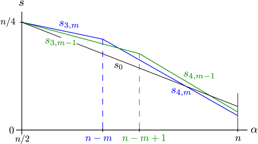
Figure 8. Comparison between $s_{m}$ and $s_{m-1}$; see Proposition 4.2i.

To prove (232), we need to discard the contribution of $m_{0}<m\leq m_{1}$ in the range $n-m_{0}\leq\alpha\leq n$. Since $s_{m_{0}}(\alpha)=s_{4,m_{0}}(\alpha)\leq s^{S}(\alpha)$ in this range of $\alpha$, then we are done if we can show that $s_{m}(\alpha)\leq s_{4,m_{0}}(\alpha)$, where $s_{m}$ is given by (219).

In the range $\beta_{m,2}\leq\alpha\leq n$ we can repeat the analysis in (236) to see that

$$m_{0}+1\leq m\leq m_{1}\quad\Longrightarrow\quad s_{m}(\alpha)=s_{4,m}(\alpha)<s_{4,m_{0}}(\alpha),\qquad\beta_{m,2}\leq\alpha\leq n.$$ (238)

If $n\in 3\mathbb{N}$ and $m=m_{0}+1$, then $\beta_{m_{0}+1,\,2}<n-m_{0}$ and we are done; otherwise, we have to consider the interval $n-m_{0}\leq\alpha\leq\beta_{m,2}$ as well.

Assume that $n\notin 3\mathbb{N}$ or that $m>m_{0}+1$. In this case,

$$\beta_{m,2}=\frac{n+m+1}{2}\geq n-m_{0}.$$ (239)

Since $s_{m}(\beta_{m,2})<s_{4,m_{0}}(\beta_{m,2})$ and $s_{m}(\alpha)=s_{5,m}(\alpha)$ for $n-m_{0}\leq\alpha\leq\beta_{m,2}$, it suffices to show that the slope of $s_{5,m}$ is greater (or less steep) than that of $s_{4,m_{0}}$, which is true because

$$-\frac{n-m-2}{2(n-m-1)}\geq-\frac{n-m_{0}}{2(n-m_{0}+1)}\iff m\geq m_{0}-2.$$ (240)

This concludes the proof of (232).

Finally, (233) holds because for $n=4,5,7$ there is no $m$ such that $m_{0}<m\leq m_{1}$. ∎

The next step is to determine the maximum regularity among the intermediate $m$.

Lemma 5.4.

Let $n=6$ or $n\geq 8$, $m_{0}=\lfloor(n-1)/3\rfloor$ and $m_{1}=\lfloor n/2-1\rfloor$. Define $s^{I}(\alpha)=\max_{m_{0}<m\leq m_{1}}s_{m}(\alpha)$. Then,

$$s^{I}(\alpha)=s_{m_{0}+1}(\alpha),\qquad\textrm{when }n=6,8,9,10,11,13,$$ (241)

and if $n=12$ or $n\geq 14$,

$$s^{I}(\alpha)=\begin{cases}s_{3,m_{1}}(\alpha)&\textrm{for }n/2\leq\alpha\leq\beta_{m_{1},1}\textrm{ and }n\textrm{ odd},\\ s_{5,m}(\alpha),&\textrm{for }\beta_{m,1}\leq\alpha\leq n-m-1+3\,\dfrac{n-2m-2}{n-m-4},\\ s_{3,m-1}(\alpha),&\textrm{for }n-m-1+3\,\dfrac{n-2m-2}{n-m-4}\leq\alpha\leq\beta_{m-1,1},\\ s_{m_{0}+1}(\alpha),&\textrm{for }\beta_{m_{0}+1,1}\leq\alpha\leq n-m_{0},\end{cases}$$ (242)

where $m$ ranges from $m_{0}+2$ to $m_{1}$.

Furthermore,

$$s(\alpha)=s^{I}(\alpha),\qquad\textrm{for }n/2\leq\alpha\leq\beta_{m_{0}+1,1}.$$ (243)

Proof.

The identity (241) holds because the interval $m_{0}<m\leq m_{1}$ only has one element for those dimensions.

To prove (242) for $n=12$ or $n\geq 14$, the analysis is like in Lemma 5.3. Recall that $s_{m}$ is given by (219) in this case, so we have to consider the transition point

$$\beta_{m,1}=n-m-1+2\frac{n-2m-2}{n-m-3}\in[n-m-1,n-m).$$ (244)

Like in (235), we see that

$$l\leq m-1\quad\Longrightarrow\quad s_{m-1}(\alpha)=s_{3,m-1}(\alpha)\geq s_{3,l}(\alpha)=s_{l}(\alpha),\qquad n/2\leq\alpha\leq\beta_{m-1,1}.$$ (245)

On the other hand, when $l\geq m$ and $\beta_{m,1}\leq\alpha\leq\beta_{m_{0}+1,1}<\beta_{m,2}$ we have

$$s_{m}(\alpha)=s_{5,m}(\alpha)\geq s_{5,l}(\alpha)=s_{l}(\alpha)\iff\frac{n-m-2}{n-m-1}\geq\frac{n-l-2}{n-l-1}\iff l\geq m.$$ (246)

Consequently,

$$s^{I}(\alpha)=\max\{s_{3,m-1}(\alpha),s_{5,m}(\alpha)\},\qquad\beta_{m,1}\leq\alpha\leq\beta_{m-1,1},$$ (247)

and the two middle cases in (242) follow.

When $n$ is even we get $\beta_{m_{1},1}=n/2$, so the computations above cover the whole range $n/2\leq\alpha\leq\beta_{m_{0}+1,1}$. When $n$ is odd, though, $\beta_{m_{1},1}>n/2$ and the first case in (242) follows from (245) by taking $m-1=m_{1}$.

Now we prove the last case in (242), that is, that $s_{m_{0}+1}(\alpha)\geq s_{m}(\alpha)$ for $m_{0}+2\leq m\leq m_{1}$ and for $\beta_{m_{0}+1,1}\leq\alpha\leq n-m_{0}$. From (219) and (239) we see that $s_{m}(\alpha)=s_{5,m}(\alpha)$, so we have to prove $s_{m_{0}+1}(\alpha)\geq s_{5,m}(\alpha)$ for $m\geq m_{0}+2$.

When $n\not\in 3\mathbb{N}$ we have $\beta_{m_{0}+1,\,2}\geq n-m_{0}$, so $s_{m_{0}+1}(\alpha)=s_{5,m_{0}+1}(\alpha)$ and we have to prove $s_{5,m_{0}+1}(\alpha)\geq s_{5,m}(\alpha)$, but this follows like in (246). When $n\in 3\mathbb{N}$, then $m_{0}=n/3-1$ and we also have to study the range

$$\beta_{m_{0}+1,\,2}=\frac{n+(m_{0}+1)+1}{2}=\frac{2n}{3}+\frac{1}{2}\leq\alpha\leq\frac{2n}{3}+1=n-m_{0}.$$ (248)

In this range $s_{m_{0}+1}(\alpha)=s_{4,m_{0}+1}(\alpha)$, so we must prove $s_{4,m_{0}+1}(\alpha)\geq s_{5,m}(\alpha)$ for $m\geq m_{0}+2$. For that, it is enough to check $s_{4,m_{0}+1}(\alpha)\geq s_{5,m_{0}+2}(\alpha)$. Since $s_{m_{0}+1}(\beta_{m_{0}+1,\,2})\geq s_{5,m_{0}+2}(\beta_{m_{0}+1,\,2})$, we only need to prove the inequality at $\alpha=2n/3+1$, which follows after algebraic manipulation.

To prove (243), by the first case in (231) it is enough to show that $s_{3,m_{0}}(\alpha)<s_{3,m_{0}+1}(\alpha)=s_{m_{0}+1}(\alpha)\leq s^{I}(\alpha)$ for $n/2\leq\alpha\leq\beta_{m_{0}+1,1}$. This follows like in (235), so we conclude the proof of the lemma. ∎

After Lemmas 5.3 and 5.4, it only remains to analyze the range $\beta_{m_{0}+1,1}\leq\alpha\leq n-m_{0}$.

Lemma 5.5.

Let $m_{0}=\lfloor(n-1)/3\rfloor$. Then,

• When $n=6$,

  $$s(\alpha)=s_{3,m_{0}}(\alpha),\qquad\textrm{for }n/2\leq\alpha\leq n-m_{0}.$$ (249)

• When $n\geq 8$,

  $$s(\alpha)=\begin{cases}s_{5,m_{0}+1}(\alpha),&\qquad\beta_{m_{0}+1,1}\leq\alpha\leq n-m_{0}-2+3\,\dfrac{n-2m_{0}-4}{n-m_{0}-5},\\ s_{3,m_{0}}(\alpha),&\qquad n-m_{0}-2+3\,\dfrac{n-2m_{0}-4}{n-m_{0}-5}\leq\alpha\leq n-m_{0}.\end{cases}$$ (250)

Proof.

From the first case in (231) and the last case in (242) we have that

$$s(\alpha)=\max\{s_{3,m_{0}}(\alpha),s_{m_{0}+1}(\alpha)\}.$$ (251)

When $n\notin 3\mathbb{N}$ then (219) and (239) imply that $s_{m_{0}+1}(\alpha)=s_{5,m_{0}+1}(\alpha)$, so

$$s(\alpha)=\max\{s_{3,m_{0}}(\alpha),s_{5,m_{0}+1}(\alpha)\},$$ (252)

which is precisely (250); notice that $n-m_{0}-5>0$ in this case. When $n\in 3\mathbb{N}$ and $n\neq 6$, then $m_{0}=n/3-1$ and

$$s(\alpha)=\begin{cases}\max\{s_{3,m_{0}}(\alpha),s_{5,m_{0}+1}(\alpha)\},&\qquad\beta_{m_{0}+1,1}\leq\alpha\leq 2n/3+1/2,\\ \max\{s_{3,m_{0}}(\alpha),s_{4,m_{0}+1}(\alpha)\},&\qquad 2n/3+1/2\leq\alpha\leq 2n/3+1,\end{cases}$$ (253)

which again leads to (250); notice that

$$n-m_{0}-2+3\,\frac{n-2m_{0}-4}{n-m_{0}-5}=\beta_{m_{0}+1,\,2}=\frac{2n}{3}+\frac{1}{2}.$$ (254)

When $n=6$, we have $s_{3,m_{0}}(\alpha)=s_{5,m_{0}+1}(\alpha)$, so we may choose $s_{3,m_{0}}$ in the first maximum above to reach (249). ∎

Gathering the results of this section, we get Theorem 1.1.

Remark 5.6.

Given that $\beta_{m,2}$ plays no role in the final statement of Theorem 1.1, for simplicity we rename $\beta_{m,1}$ as $\beta_{m}$.

References

- [1] An, C., Chu, R., and Pierce, L. B. Counterexamples for high-degree generalizations of the Schrödinger maximal operator. https://arxiv.org/abs/2103.15003.
- [2] Barceló, J. A., Bennett, J., Carbery, A., and Rogers, K. M. On the dimension of divergence sets of dispersive equations. Math. Ann. 349, 3 (2011), 599–622.
- [3] Beresnevich, V., and Velani, S. A mass transference principle and the Duffin-Schaeffer conjecture for Hausdorff measures. Ann. of Math. (2) 164, 3 (2006), 971–992.
- [4] Bourgain, J. On the Schrödinger maximal function in higher dimension. Tr. Mat. Inst. Steklova 280 (2013), 53–66.
- [5] Bourgain, J. A note on the Schrödinger maximal function. J. Anal. Math. 130 (2016), 393–396.
- [6] Carleson, L. Some analytic problems related to statistical mechanics. In Euclidean harmonic analysis (Proc. Sem., Univ. Maryland, College Park, Md., 1979) (1980), vol. 779 of Lecture Notes in Math., Springer, Berlin, pp. 5–45.
- [7] Cho, C.-H., and Lee, S. Dimension of divergence sets for the pointwise convergence of the Schrödinger equation. J. Math. Anal. Appl. 411, 1 (2014), 254–260.
- [8] Cho, C.-H., Lee, S., and Vargas, A. Problems on pointwise convergence of solutions to the Schrödinger equation. J. Fourier Anal. Appl. 18, 5 (2012), 972–994.
- [9] Compaan, E., Lucà, R., and Staffilani, G. Pointwise convergence of the Schrödinger flow. Int. Math. Res. Not. IMRN, 1 (2021), 599–650.
- [10] Dahlberg, B. E. J., and Kenig, C. E. A note on the almost everywhere behavior of solutions to the Schrödinger equation. In Harmonic analysis (Minneapolis, Minn., 1981), vol. 908 of Lecture Notes in Math. Springer, Berlin-New York, 1982, pp. 205–209.
- [11] Du, X. Upper bounds for Fourier decay rates of fractal measures. J. Lond. Math. Soc. (2) 102, 3 (2020), 1318–1336.
- [12] Du, X., Guth, L., and Li, X. A sharp Schrödinger maximal estimate in . Ann. of Math. (2) 186, 2 (2017), 607–640.
- [13] Du, X., Kim, J., Wang, H., and Zhang, R. Lower bounds for estimates of the Schrödinger maximal function. Math. Res. Lett. 27, 3 (2020), 687–692.
- [14] Du, X., and Zhang, R. Sharp estimates of the Schrödinger maximal function in higher dimensions. Ann. of Math. (2) 189, 3 (2019), 837–861.
- [15] Eceizabarrena, D., and Lucà, R. Convergence over fractals for the periodic Schrödinger equation. Anal. PDE, To Appear. https://arxiv.org/abs/2005.07581.
- [16] Eceizabarrena, D., and Ponce-Vanegas, F. Pointwise convergence over fractals for dispersive equations with homogeneous symbol. https://arxiv.org/abs/2108.10339.
- [17] Falconer, K. Fractal geometry, second ed. John Wiley & Sons, Inc., Hoboken, NJ, 2003. Mathematical foundations and applications.
- [18] Hardy, G. H., and Wright, E. M. An introduction to the theory of numbers. Edited and revised by D. R. Heath-Brown and J. H. Silverman. With a foreword by Andrew Wiles. 6th ed, 6th ed. ed. Oxford: Oxford University Press, 2008.
- [19] Lee, S. On pointwise convergence of the solutions to Schrödinger equations in . Int. Math. Res. Not. (2006), Art. ID 32597, 21.
- [20] Li, W., Wang, H., and Yan, D. A note on non-tangential convergence for Schrödinger operators. J. Fourier Anal. Appl. 27, 4 (2021), Paper No. 61, 14.
- [21] Li, Z., Zhao, J., and Zhao, T. schrödinger maximal estimates associated with finite type phases in . https://arxiv.org/abs/2111.00897.
- [22] Lucà, R., and Ponce-Vanegas, F. Convergence over fractals for the Schrödinger equation. Indiana Univ. Math. J., To Appear. https://arxiv.org/abs/2101.02495.
- [23] Lucà, R., and Rogers, K. M. Average decay of the Fourier transform of measures with applications. J. Eur. Math. Soc. (JEMS) 21, 2 (2019), 465–506.
- [24] Lucà, R., and Rogers, K. M. A note on pointwise convergence for the Schrödinger equation. Math. Proc. Cambridge Philos. Soc. 166, 2 (2019), 209–218.
- [25] Moyua, A., Vargas, A., and Vega, L. Schrödinger maximal function and restriction properties of the Fourier transform. Internat. Math. Res. Notices, 16 (1996), 793–815.
- [26] Pierce, L. B. On Bourgain’s counterexample for the Schrödinger maximal function. Q. J. Math. 71, 4 (2020), 1309–1344.
- [27] Sjögren, P., and Sjölin, P. Convergence properties for the time-dependent Schrödinger equation. Ann. Acad. Sci. Fenn. Ser. A I Math. 14, 1 (1989), 13–25.
- [28] Sjögren, P., and Sjölin, P. Convergence properties for the time-dependent Schrödinger equation. Ann. Acad. Sci. Fenn. Ser. A I Math. 14, 1 (1989), 13–25.
- [29] Sjölin, P. Regularity of solutions to the Schrödinger equation. Duke Math. J. 55, 3 (1987), 699–715.
- [30] Vega, L. Schrödinger equations: pointwise convergence to the initial data. Proc. Amer. Math. Soc. 102, 4 (1988), 874–878.
- [31] Žubrinić, D. Singular sets of Sobolev functions. C. R. Math. Acad. Sci. Paris 334, 7 (2002), 539–544.
- [32] Wang, B., and Wu, J. Mass transference principle from rectangles to rectangles in Diophantine approximation. Math. Ann. (2021).
- [33] Wang, X., and Zhang, C. Pointwise convergence of solutions to the Schrödinger equation on manifolds. Canad. J. Math. 71, 4 (2019), 983–995.