Efficient labeling algorithms for adjacent quadratic shortest paths

Abstract

In this article, we study the Adjacent Quadratic Shortest Path Problem (AQSPP), which consists in finding the shortest path on a directed graph when its total weight component also includes the impact of consecutive arcs. We provide a formal description of the AQSPP and propose an extension of Dijkstra’s algorithm (that we denote aqD) for solving AQSPPs in polynomial-time and provide a proof for its correctness under some mild assumptions. Furthermore, we introduce an adjacent quadratic A^* algorithm (that we denote aqA^*) with a backward search for cost-to-go estimation to speed up the search. We assess the performance of both algorithms by comparing their relative performance with benchmark algorithms from the scientific literature and carry out a thorough collection of sensitivity analysis of the methods on a set of problem characteristics using randomly generated graphs. Numerical results suggest that: (i) aqA^* outperforms all other algorithms, with a performance being about 75 times faster than aqD and the fastest alternative; (ii) the proposed solution procedures do not lose efficiency when the magnitude of quadratic costs vary; (iii) aqA^* and aqD are fastest on random graph instances, compared with benchmark algorithms from scientific literature. We conclude the numerical experiments by presenting a stress test of the AQSPP in the context of real grid graph instances, with sizes up to $16\times 10^{6}$ nodes, $64\times 10^{6}$ arcs, and $10^{9}$ quadratic arcs.

Keywords Shortest Path Problem  $\cdot$ Adjacent Quadratic Shortest Path Problem  $\cdot$ Backward Cost-to-Go Estimation  $\cdot$ $\alpha$-Cycle  $\cdot$ Spatial Routing

1 Introduction

Finding the least-weighted path between two vertices in a graph is a well-studied problem in computer science and has been deeply explored in the technical literature both from a methodological perspective (Pollack and Wiebenson, 1960; Ahuja et al., 1993; Madkour et al., 2017) as well as from an applied point of view (Duque et al., 2015; Hougardy et al., 2017; Furini et al., 2020; Ru$\beta$ et al., 2021). This problem is usually referred to as the Shortest Path Problem (SPP) and aims at finding a path $P$ on a weighted graph $G=(V,A,\boldsymbol{c})$ that connects a source node $s\in V$ with a target node $t\in V$ of minimal total weight. Structurally, the SPP can be formulated as an integer programming problem with a linear objective function $\boldsymbol{c}^{\top}\mathbf{x}$, where $\boldsymbol{c}\in\mathbb{R}^{|A|}$ represents an edges-wise weight vector and $\mathbf{x}\in\{0,1\}^{|A|}$ indicates a binary vector of arc selections, constrained to a network-flow-based feasible region, that builds up the shortest path (Taccari, 2016). Many procedures have been developed over the past decades to solve the SPP efficiently (e.g., Bellman-Ford (Bellman, 1958), Floyd-Warshall (Floyd, 1962), and A^* (Hart et al., 1968) algorithms), with the most well-known approach due to Dijkstra (Dijkstra, 1959).

Although the linear nature of SPPs can accommodate a large collection of problem structures, some applications demand more complex interactions and cost-impacts between edges within the path, as, for instance, the problems of establishing network protocols (Murakami and Kim, 1997), optimizing vehicle routing (Martinelli and Contardo, 2015), and identifying variance-constrained shortest paths (Sivakumar and Batta, 1994; Sen et al., 2001), all intrinsically following a quadratic order. In this context, the Quadratic Shortest Path Problem (QSPP) emerges as a powerful modeling tool to properly characterize a broader class of problems since it extends the standard SPP structure by identifying a path that jointly minimizes both the total path weight and the sum of interaction costs over distinct pairs of edges on the path. Formally, the QSPP can be stated over a weighted digraph $G=(V,A,\boldsymbol{c},\boldsymbol{q})$ as a quadratic integer programming problem (Gill and Wong, 2015) with objective function defined as $\mathbf{x}^{\top}\boldsymbol{q}\mathbf{x}+\boldsymbol{c}^{\top}\mathbf{x}$, where $\boldsymbol{q}\in\mathbb{R}^{|A|}\times\mathbb{R}^{|A|}$ is a square matrix that maps the weight impact of pair of arcs and $(\boldsymbol{c},\mathbf{x})$ follows similarly to the SPP formulation (Rostami et al., 2015). In this work, we focus on a particular structure of QSPPs, referred to in technical literature as the Adjacent Quadratic Shortest Path Problem (AQSPP), which follows the same quadratic structure, but in which the matrix $\boldsymbol{q}$ only accounts for interactions among adjacent arcs.

The theory and applicability of QSPP/AQSPP have been studied through the seminal work of Amaldi et al. (2011) and further extended by Rostami et al. (2015, 2018), Hu and Sotirov (2018b, a) and Buchheim and Traversi (2018). Amaldi et al. (2011) investigated the issues over complexity and approximability in problems that seek for optimum paths, tours, and flows under the so-called reload costs, defined as the cost incurred by the path when two adjacent arcs are of “different types”. Moreover, Buchheim and Traversi (2018) explores the more general framework of Binary Quadratic Problems (BQPs) and propose an exact algorithm for this class of optimization problems based on computing quadratic global underestimators and embedding the resulting lower bounds into branch-and-bound techniques. Rostami et al. (2015) provides an in-depth mathematical description of QSPPs and proposes an algorithm to solve AQSPPs in polynomial-time based on a procedure that reduces the AQSPP to an instance of the SPP by modifying the original graph. Furthermore, Hu and Sotirov (2018a) also characterize QSPPs mathematically and derive an algorithm that examines whether QSPP instances of directed grid graphs are “linearizable”. More precisely, the authors evaluate when a grid graph with quadratic cost can be transformed into a graph with linear costs. They also reviewed the developments presented by Rostami et al. in Rostami et al. (2015) and prove that, despite stated in Rostami et al. (2015), their algorithm does not find optimal solutions in polynomial time for general digraphs, but rather only for the particular case of acyclic digraphs.

Therefore, following this latter observation and technical issue, in this work, we study computationally efficient solution methods to solve AQSPPs on a broader class of graphs, the ones that do not possess improving $\alpha$-cycles, defined as follows.

Definition 1

An $\alpha$-cycle is a walk $(u_{1},\ldots,u_{n})$ in the underlying graph with $n\geq 5$ such that $u_{2}=u_{n-1}$. An $\alpha$-cycle is said to be improving if its total compounded weight is lower than that of the shorter sequence $(u_{1},u_{2},u_{n})$.

Note that an improving $\alpha$-cycle may exist even without negative weights due to their quadratic nature. In Figure 1, we depict an $\alpha$-cycle of five nodes. The $\alpha$-cycle depicted in this figure would be improving if, for instance, one had a substantial quadratic weight impact for the sequence $(1,2,5)$ and very low for all other ones. We argue that graphs with no improving $\alpha$-cycles are more general than acyclic ones since, by definition, the latter do not possess $\alpha$-cycles, but the opposite does not hold. These types of graphs are found in several practical applications, as, for instance, on graphs that represent spatial attributes (terrain, distance, slope, etc.), wildly used on route-design problems (Wan et al., 2011; Ebrahimipoor et al., 2009; Bärmann et al., 2015; Piveteau, 2017).

Figure 1: An $\alpha$-cycle of five nodes

This work aims to contribute to the scientific literature on AQSPPs by designing an extension of Dijkstra’s algorithm (from now on referred to as aqD) to solve AQSPP on graphs with no improving $\alpha$-cycles. More specifically, we demonstrate that our algorithm finds optimal walks (paths possibly with cycles) in the absence of negative weights and acyclic paths when the graph is free of improving $\alpha$-cycles. An acceleration to the algorithm is also proposed: an adjacent quadratic A^* with a backward search for cost-to-go estimation (hereinafter referred to as aqA^*). We perform a thorough computational campaign to analyze the proposed algorithms’ performances. First, we measure the relative speed of aqD and aqA^* against the linearization-based algorithm designed in Rostami et al. (2015, 2018). Next, we analyze the sensitivity of our methods to variations in the quadratic weight levels. Then, we empirically evaluate the performance of our two algorithms on randomly generated graphs using the Erdős-Rényi (Erdős and Rényi, 1959; Bollobás, 2001) and Configuration Model (Newman, 2010) methods. The instances used for these computational tests range from $6\times 10^{5}$ to $6.4\times 10^{7}$ quadratic arcs. Finally, we stress the search process by increasing the graph sizes up to $16\times 10^{6}$ nodes, $64\times 10^{6}$ arcs, and $10^{9}$ quadratic arcs.

The outline of this work is as follows. In the next section, we present the formal problem definition with a quadratic formulation for the AQSPP. In Section 3, we introduce the extension of the classical Dijkstra’s algorithm for the adjacent quadratic case and provide a proof for its correctness in the absence of improving $\alpha$-cycles. Section 4 extends the proposed solution procedure using a cost-to-go estimation to obtain an A^* algorithm. Section 5 describes how to speed up the algorithm even further by calculating the quadratic costs on the fly to handle vary-large scale AQSPPs instances. In Section 6, we compare the proposed algorithms against benchmark approaches from scientific literature using different graph types. Finally, Section 7 concludes this work and points the avenues of future research.

2 Problem Definition

The AQSPP is defined over a weighted digraph $G=(V,A,\boldsymbol{c},\boldsymbol{q})$, where $(V,A)$ denote the sets of nodes and arcs of the network, respectively, $\boldsymbol{c}\in\mathbb{R}_{+}^{|A|}$ stands for the vector of linear costs, and $\boldsymbol{q}\in\mathbb{R}_{+}^{|A|\times|A|}$ represents the respective matrix of quadratic costs, where we assume that $q(a_{1},a_{2})=0$ if $h(a_{1})\neq t(a_{2})$, where the functions $t(\cdot)$ and $h(\cdot)$ stand for the head and the tail of an arc, respectively. This assumption allows us to overload the notation and denote $q(u,v,w)$ instead of $q((u,v),(v,w))$ for every pair of consecutive arcs in $A\times A$. In addition to $G$, we are also given a source node $s\in V$ and a target node $t\in V\setminus\{s\}$. For every node $u\in V$ we denote $\delta^{+}(u)=\{a\in A:t(a)=u\}$ and $\delta^{-}(u)=\{a\in A:h(a)=u\}$.

The AQSPP can be formulated as a binary quadratic program (BQP), as presented in (1)–(3). We are given, for every arc $a\in A$, a binary variable $x_{a}$ that takes the value 1 if $a$ is part of the shortest path. The following BQP is valid for the AQSPP:

$$\min_{\mathbf{x}}\quad\sum_{a\in A}c(a)x_{a}+\sum_{(a,b)\in A\times A}q(a,b)x_{a}x_{b}$$ (1)

subject to

$$\sum_{a\in\delta^{+}(u)}x_{a}-\sum_{a\in\delta^{-}(u)}x_{a} =\begin{cases}1&\hskip 14.22636ptu=s\\ -1&\hskip 14.22636ptu=t\\ 0&\hskip 14.22636ptu\in V\setminus\{s,t\}\end{cases} u\in V$$ (2)

$$x_{a} \in\{0,1\} a\in A.$$ (3)

Note that the feasible region defined by (2)-(3) on the AQSPP formulation is equivalent to the standard SPP (Taccari, 2016). Thus, all paths that are feasible for one of them, are also for the other. The main difference between the linear and the quadratic case comes from introducing the quadratic term $q(a,b)x_{a}x_{b}$ in the objective function (1). Due to the total unimodularity characteristic of the constraint matrix, one may be tempted to drop the integrality constraints for the binary variables. However, note that unlike the linear case, an interior point may now be optimal in the AQSPP, justifying the need for the integrality constraints (3) for the $\mathbf{x}$-variables.

It should be highlighted that using BQP techniques to solve the AQSPP seems a reasonable approach and has already been explored in the scientific literature (Buchheim and Traversi, 2018; Caprara, 2008). However, we argue that as the size of the graph grows, using off-the-shelf solvers without exploiting the underlying shortest path structure of the problem may quickly become prohibitive. Memory issues that raise from building up a very heavy optimization problem can easily occur and prevent the solver from providing meaningful results. Additionally, the performance of BQP solvers in large instances can quickly deteriorate. These limitations motivate us to study this problem from an algorithmic perspective, to ultimately introduce two algorithms to solve AQSPPs. Both algorithms are described in Sections 3 and 4.

3 Adjacent Quadratic Dijkstra

In this section, we describe a dynamic programming algorithm for the AQSPP, referred to in this work as the adjacent quadratic Dijkstra (aqD). The algorithm is based on the concept of node labels and can adequately address adjacent costs.

3.1 The Algorithm

The Adjacent Quadratic Dijkstra algorithm proposed in this work follows a similar structure to the standard Dijkstra’s algorithm, but computing the shortest distances between the source and every possible arc in the network, as opposed to the standard Dijkstra solution method that computes the minimum costs between the source and every possible node in the network. More specifically, for a given source node $s\in V$ and an arc $a=(i,j)\in A$, we define a $s$-$a$-walk as a tuple $(v_{0},v_{1},\ldots,v_{k})$ such that $v_{0}=s,v_{k-1}=i,v_{k}=j$, and let us to denote by $D_{a}$ the cost of the best $s$-$a$-walk. This notation allows computing adjacent costs when extending a walk that ends at arc $a$. We present a pseudo-code of the solution method in Algorithm 1.

Algorithm 1 Adjacent Quadratic Dijkstra

1:function aqDikstra($V,A,c,q,s$):

2:

3:Let $D_{a}\leftarrow+\infty$ for every $a\in A$

4:Let $D_{(s,s)}\leftarrow 0$, $Q\leftarrow\{(s,s)\}$

5:

6:while $Q\neq\emptyset$ do

7:     Let $a=(i,j)\in\arg\min\{D_{a}:a\in Q\}$

8:     Set $Q\leftarrow Q\setminus\{a\}$

9:     for each $k$ in neighbors of $j$ do

10:         if $D_{a}+c_{jk}+q_{ijk}<D_{(j,k)}$ then

11:              Set $D_{(j,k)}\leftarrow D_{a}+c_{jk}+q_{ijk}$

12:              Set $Q\leftarrow Q\cup\{(j,k)\}$               

13:return $D$

The iteration over the arcs is controlled by a priority queue $Q$. Priority queues are abstract data types similar to stacks in which each element has a priority assigned to it. These queue structures are often used to speed up the search and are the standard on most implementations of Dijkstra’s algorithm. The element with the highest priority is always positioned on top of the stack, forcing it to be the first to be removed. In this case, the labels with smallest accumulated costs should be prioritized since they indicate shorter paths and should be positioned on top of the stack. At each iteration, the arc $a\in A$ with the smallest cumulative cost $D_{a}$ is removed from $Q$ and used as a reference to explore the neighboring nodes. Each neighbor $k$ is then evaluated and its associated cumulative cost updated according to an update criterion. The algorithm stops when $Q$ becomes empty.

The following results demonstrate the correctness of our method to compute optimal walks in the absence of negative costs and optimal acyclic paths if the graph is free of improving $\alpha$-cycles.

Proposition 1

If $c,q\geq 0$, the algorithm ends in a finite number of iterations and computes, for every arc $a=(i,j)\in A$, the cost of a minimum $s$-$a$-walk.

Proof 1

The number of iterations of the algorithm is governed by the times an arc $a\in\arg\min\{D_{a}:a\in Q\}$ is selected at Line 7. We denote $a_{t}$ the arc selected at this line at iteration $t$ of the algorithm. Let us define $R_{0}=\emptyset$ and for every $t\geq 1$, $R_{t}\leftarrow R_{t-1}\cup\{a_{t}\}$. With these definitions, we have that $a_{1}=(s,s),R_{1}=\{(s,s)\}$.

We will first demonstrate that, for every $t\geq 1$, $a_{t}\notin R_{t-1}$. The first time an arc $a_{t}=a^{*}$ is added to $R_{t}$, it satisfies $D_{a^{*}}\leq D_{a}$ for every $a\in Q$. Since the components of $c,q$ are non-negative by assumption, it follows that any extension of any walk can only increase its cost. By the time another walk is extended using the arc $a^{*}$, its cost can only be $\geq D_{a^{*}}$. This means the cost of $D_{a^{*}}$ will never be updated, and therefore $a^{*}$ will never enter the priority queue $(Q)$ again.

We will now prove that, at iteration $t$, $D_{a_{t}}$ is the cost of the shortest $s$-$a_{t}$-walk. The result is obviously true for $t=1$. Let us assume by induction that the result holds for $t$, and let us assume by contradiction that there exists a walk $w=(w_{1}=s,\ldots,w_{l-1}=i_{t+1},w_{l}=j_{t+1})$ such that $c(w)<D_{a_{t+1}}$, where $a_{t+1}=(i_{t+1},j_{t+1})$. Let $k$ be the first index in this walk such that $(w_{k},w_{k+1})\notin R_{t}$ (this is well defined since $a_{t+1}$ satisfies this property). Let $pw_{k}=(w_{1}=s,\ldots,w_{k})$ be the $k$-th prefix of walk $w$. Since the components of $c,q$ are non-negative by assumption, it follows that $c(pw_{k})+c_{w_{k}w_{k+1}}+q_{w_{k-1}w_{k}w_{k+1}}\leq c(w)$. Also, because $(w_{k-1},w_{k})\in R_{t}$, the induction hypothesis implies that $D_{w_{k-1}w_{k}}\leq c(pw_{k})$. Now, because $w_{k+1}$ is adjacent to $(w_{k-1},w_{k})$ in $w$, it follows from the labeling algorithm that $D_{w_{k}w_{k+1}}\leq D_{w_{k-1}w_{k}}+c_{w_{k}w_{k+1}}+q_{w_{k-1}w_{k}w_{k+1}}$. Finally, because $a_{t+1}$ was picked at iteration $t+1$ of the algorithm and because $(w_{k},w_{k+1})\notin R_{t}$, it follows that $D_{a_{t+1}}\leq D_{w_{k}w_{k+1}}$. We put all these inequalities together to obtain:

$$D_{a_{t+1}} \leq D_{w_{k}w_{k+1}}$$

$$\leq D_{w_{k-1}w_{k}}+c_{w_{k}w_{k+1}}+q_{w_{k-1}w_{k}w_{k+1}}$$

$$\leq c(pw_{k})+c_{w_{k}w_{k+1}}+q_{w_{k-1}w_{k}w_{k+1}}$$

$$\leq c(w)$$

$$<D_{a_{t+1}},$$

which is obviously a contradiction, proving that $D_{a_{t+1}}$ is the minimum cost among all $s$-$a_{t+1}$-walks.$\hfill\square$

Proposition 2

In the absence of improving $\alpha$-cycles, $\min\{D_{a}:a\in\delta^{-}(t)\}$ as computed by Algorithm 1 corresponds to the minimum cost of a $s$-$t$-path in $G$.

Proof 2

Let us assume by contradiction that, for a given arc $a=(u,t)$, $D_{a}$ corresponds to the cost of a $s$-$a$-walk with a cycle and that no $s$-$a$-path exists with the same cost. This walk can be written as $(w_{i})_{i=1}^{n}$ with $w_{1}=s,w_{n-1}=u,w_{n}=t$ and $(w_{i},w_{i+1})\in A$ for every $i=1\ldots n-1$. If $w_{l}=w_{k}$ for $1<l<k<n$, one can replace the $\alpha$-cycle $(w_{i})_{i=l-1}^{k+1}$ by $(w_{l-1},w_{l},w_{k+1})$ to obtain a walk with one less cycle, at the same cost or less (because the $\alpha$-cycle is non-improving). One can repeat this argument as many times as necessary to ultimately obtain a $s$-$a$-path of the same cost or less, which contradicts our assumption. It follows that $D_{a}$ corresponds to the cost of a $s$-$a$-path.$\hfill\square$

These two results characterize a nice feature of our method. One does not need to incur into an expensive procedure to check for the existence of improving $\alpha$-cycles. Instead, one can check for the non-negativity of the graph weights and execute the aqD regardless of the existence of $\alpha$-cycles. One can a posteriori check for the existence of improving $\alpha$-cycles once the algorithm has computed an optimal $s$-$t$-walk.

3.2 Complexity of aqD

The number of neighboring arcs that are inspected in Line 10 is bounded above by the number of quadratic arcs of the form $(i,j,k)$ with $\big{(}(i,j),(j,k)\big{)}\in A\times A$, that we denote $|A_{Q}|$. Removing the arc of highest priority from $Q$ and rearranging its elements to maintain its structure can be done in $\mathcal{O}(\log|A|)$ amortized time if the priority queue is implemented using a heap. The total number of iterations (governed by the main loop in Line 6 of the pseudo-code) is $\mathcal{O}(|A|)$. This leads to a total complexity of $\mathcal{O}(|A|\log|A|+|A_{Q}|)$. For dense graphs (those for which $\mathcal{O}(|A_{Q}|)=\mathcal{O}(V^{3})$ and $\mathcal{O}(|A|)=\mathcal{O}(V^{2})$), the time complexity is of $\mathcal{O}(V^{3})$. On sparse graphs (those for which $\mathcal{O}(|A|)=\mathcal{O}(|A_{Q}|)=\mathcal{O}(|V|)$), the time complexity is reduced to $\mathcal{O}(|V|\log|V|)$. For comparison, the standard Dijkstra’s method for linear shortest paths runs in $\mathcal{O}((|A|+|V|)\log|V|)$ time using a heap, which reduces to $\mathcal{O}(|V|^{2}\log|V|)$ for dense graphs, and to $\mathcal{O}(|V|\log|V|)$ for sparse ones. Hence our algorithm shares the same worst-case complexity as the standard Dijkstra’s method on sparse graphs, but is slower on dense graphs.

4 A^* with backward search for cost-to-go estimation

In this section, we introduce a bidirectional labeling algorithm to increase the search speed. This scheme consists in solving the problem in two steps: (i) a backward search using a (linear) SPP, starting from the target node $t\in V$, to find cost-to-go estimates; (ii) a forward search for the original AQSPP, starting from the source node $s\in V$, but considering the cost-to-go estimates as lower bounds to guide the search. This approach is inspired by the work of Thomas et al. (2019), where the authors extend the seminal work of Hart et al. (1968) to develop a bidirectional search for resource-constrained shortest path problems. The idea is built upon Hart et al.’s demonstration that A^* only terminates with an optimal path when the estimates of the cost-to-go are actual lower bounds. In the context of this work, for the case of a quadratic shortest path search, linear estimators of the costs-to-go are actual lower bounds for the quadratic problem provided that the quadratic terms are reduced — or as in this case, ignored. The fundamental idea is that these linear estimations can be calculated through a backward search from the target node $t\in V$ to all other nodes by solving the standard (linear) SPP.

Structurally, the algorithm starts with a backward search for the linear SPP where the quadratic costs are neglected. Starting from the sink node $t\in V$, one finds, for every node $u\in V$, the shortest distance from $u$ to $t$ using the linear costs $\boldsymbol{c}$. We denote $(B_{u})_{u\in V}$ the costs computed using this procedure. Note that the algorithm not only is fast even for dense graphs (it relies on solving the standard SPP using Dijkstra’s method) but also occupies only linear space to store the information. Note that this method also provides an upper bound for the AQSPP by evaluating the $s$-$t$-path solution provided by considering the quadratic costs.

In the second step, we perform a forward search using the proposed aqD method but taking into account the cost-to-go estimators to guide the search. More specifically, for every arc $a=(i,j)\in A$, $D_{a}+B_{j}$ represents a lower bound on the cost that would be achieved by extending the current $s$-$a$-walk to $t\in V$. These values are then used to select the next arc to process in the aqD method. By estimating the cost of arriving at $t\in V$, we can significantly reduce the size of the search tree and speed up the procedure. However, it is important to be aware that these estimates must always correspond to lower bounds on the costs-to-go to guarantee the correctness of the method.

The proposed method is presented on Algorithm 2.

Algorithm 2 Adjacent Quadratic A^* with backward cost-to-go estimation

1:function aqA^*($G$,$c$,$q$,$s$,$t$):

2:

3:Let $(B_{u})_{u\in V}\leftarrow Dijkstra(G,c,t)$

4:Let $D_{a}\leftarrow+\infty$ for every $a\in A$

5:Let $D_{(s,s)}\leftarrow 0$, $Q\leftarrow\{(s,s)\}$

6:

7:while $Q\neq\emptyset$ do

8:     Let $a=(i,j)\in\arg\min\{D_{a}+B_{j}:a=(i,j)\in Q\}$

9:     Set $Q\leftarrow Q\setminus\{a\}$

10:     for each $k$ in neighbors of $j$ do

11:         if $D_{a}+c_{jk}+q_{ijk}<D_{(j,k)}$ then

12:              Set $D_{(j,k)}\leftarrow D_{a}+c_{jk}+q_{ijk}$

13:              Set $Q\leftarrow Q\cup\{(j,k)\}$               

14:return $D$

5 Solving very-large scale AQSPPs in practice

On both proposed algorithms — aqD and aqA^* —, the adjacent quadratic cost matrix $\boldsymbol{q}$ are assumed to be pre-calculated and allocated on some existing data structure. Although having such information allocated in memory improves the search speed of the algorithm, it can become impractical as the problems increase in size. For instance, when dealing with very-large-scale road networks, the graphs can easily achieve dimensions of millions of nodes, tens of millions of arcs, and hundreds of millions of quadratic arcs. Thus, storing this information in memory becomes impractical.

In this section, we propose a follow-on improvement to aqD and aqA^*, which embeds the assessment of the adjacent quadratic costs within the algorithms (on the fly). This is possible whenever there exists a function $\Gamma:V^{3}\rightarrow R^{+}$ able to compute quadratic costs for every three indices $(i,j,k)$. We will refer to these modified algorithms as aqD+ and aqA^*+.

Several applications could benefit from this improvement and could build a function like $\Gamma$. The problem of spatially defining a route, for example, often requires path search on massive instances. Those problems usually use three-dimensional spatial data, which can be converted into extensive graphs used to define the routes. Additionally, attributes such as slope, angle, and others can be used as input for $\Gamma$ due to their psychical nature. Large infrastructure projects, such as highways, electric transmission lines, and gas pipelines rely on this framework.

6 Computational Experiments

In this section, we focus on evaluating the performance of the proposed algorithms, presenting results from a set of computational experiments. We explore random graph instances generated with two different methods and observe their effects on the search behavior. Then, we analyze the algorithms’ sensitivity to variations of the quadratic cost. On the third test, we compare the algorithms’ performance on real grid instances with different sizes. Finally, the last experiment perform a stress test, where we increase instances sizes up to $16\times 10^{6}$ nodes, $64\times 10^{6}$ arcs, and $10^{9}$ quadratic arcs.

The computational analyses evaluate the total search time required by the proposed algorithms against the method presented in Rostami et al. (2015) and reviewed in Hu and Sotirov (2018a) that solves AQSPPs for directed acyclic graphs. This algorithm re-writes the original graph according to a linearization of adjacent quadratic costs. Thus, the optimal path can be found on an extended graph through standard SPP algorithms. We will refer to this benchmark as Lin in the following sections. The results from solving the BQP using off-the-shelf solvers are not presented due to the solver’s inability to handle even the smallest instance tested in our experiments.

6.1 Software and Machine Settings

The Julia programming language is used throughout this work. The package Graphs.jl (Fairbanks et al., 2021) is chosen to handle graph data structures, as it provides efficient data structures to handle graph objects and mature methods to solve shortest path problems. It should be highlighted that our implementation of the aqD algorithm is made on top of Dijkstra’s algorithm implementation provided by this package.

The R programming language was also used in this paper, mainly for Geographic Information System (GIS) purposes. The packages rgdal and rgeos were used for manipulation of geographical data that was further converted into the graphs used for the computational experiments and the application study. All source code used in this work is publicly available for further verification, validation, and improvements. Finally, computational calculations were made on an Intel^® Core i7-10700K 4.8GHz with 64 GB of RAM machine, using one single thread.

6.2 Random graphs

In the first experiment, we study the algorithms’ performance considering randomly generated graph instances. We aim to analyze with this experiment how does random graphs topology impacts the search process. The methods used to build the instances are known as Erdős-Rényi (Erdős and Rényi, 1959; Bollobás, 2001) and Configuration Model (Newman, 2010), which have been widely used in scientific literature. More specifically, the Erdős-Rényi methods defines a graph where the arcs are added between pairs of nodes according to a given probability $p\in[0,1]$. The greater $p$ is, greater is the number of arcs, thus the denser the graph is. For expository purposes, in this model, we define $p$ as $0.8$ to obtain highly connected instances and range the number of nodes $|V|\in\{100,150,200,250,300,350,400\}$. For each configuration $(|V|,p)$, 100 random instances are generated. Costs for arcs and quadratic arcs are also randomly generated using a standard Uniform distribution, i.e., $\big{(}q(i,j,k),c\big{(}(i,j)\big{)}\big{)}\sim Unif(0,1)$.

Figure 2 presents compiled results from this experiment, showcasing the minimum, average, and maximum search times for each algorithm and size tested. One can notice a clear variation in search time for each of the tested algorithms. Results for aqA^* and aqD show reduced and similar search-times throughout the instances. This behavior can be explained by the high connectivity of the Erdős-Rényi instances considered in this experiment. Since $p$ was set to $0.8$, there is a high probability that the source node is close-connected to the target node, thus the shortest path contains only a few nodes. Consequently, the number of nodes needed to be visited becomes small, shortening the search process.

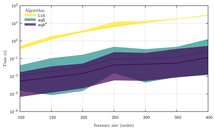
Figure 2: Results for Erdős-Rényi instances

Furthermore, we highlight the difference in the search-time magnitude for the benchmark Lin approach, in comparison to aqA^* and aqD. This difference is primarily due to the time spent building the linearized graph. Since the number of quadratic arcs is large, performing the linearization is very time-consuming and becomes a drawback to this approach.

The Configuration Model generates a random graph $G$ from a given degree sequence $\boldsymbol{\kappa}=\{\kappa_{i}\}_{i=1}^{|V|}$. A degree defines the number of connections a given node has, therefore, as $\boldsymbol{\kappa}$ increases, so does the number of arcs in $G$. To build the graph, the method randomly samples $\kappa_{i}$ nodes from $G$ and connects them to node $i\in V$. For this model, we fix the nodes’ degrees to $8$ and vary the number of nodes $|V|\in\{150\times 10^{3},200\times 10^{3},250\times 10^{3},300\times 10^{3}\}$. Similarly, 100 random instances are generated with $c\big{(}(i,j)\big{)}$ and $q(i,j,k)$ drawn from an $Unif(0,1)$. Results from the Configuration Model, presented in Figure 3, suggest that the speed ups remain nearly constant, with our method aqA^* performing around 32 times faster on average than Lin. Additionally, aqD is about 5 times faster than Lin.

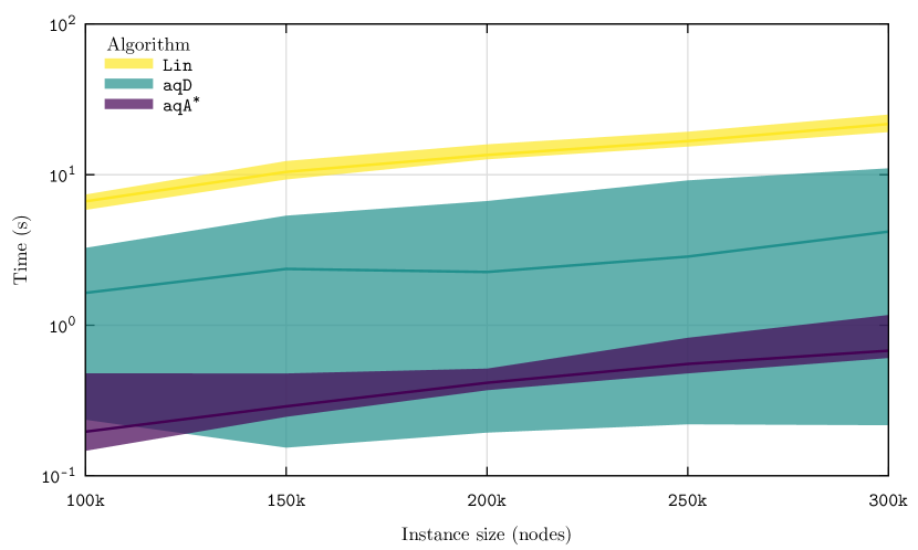
Figure 3: Results for Configuration Model instances

Furthermore, the presented results indicate that the aqA^* exhibits less variance than aqD, resulting in a more consistent and predictable search time for instances generated with the Configuration Model. These results reaffirm the role of the backward step on providing reasonable cost-to-go estimates and consistently speeding up the search process.

6.3 Quadratic Cost Variation

The second experiment measures the sensitivity of the algorithms to the magnitude of quadratic costs. A parameter $\lambda\in\{1,5,50,500,1000\}$ is set to scale the quadratic costs, so that the arc interaction would be $\lambda q(i,j,k)$. We test $100$ instances generated with the Erdős-Rényi method with $400$ nodes and $100$ instances generated with the Configuration Model with $300\times 10^{3}$ nodes for each $\lambda$ value. Figures 4 and 5 present total search time for both graphs, and for each $\lambda$ value considered. The presented results suggest that aqA^*, aqD and Lin are not significantly influenced by an increase of quadratic costs. We also do not observe any apparent trends or unconventional behaviour on the plots, confirming the insensitivity towards quadratic cost variation.

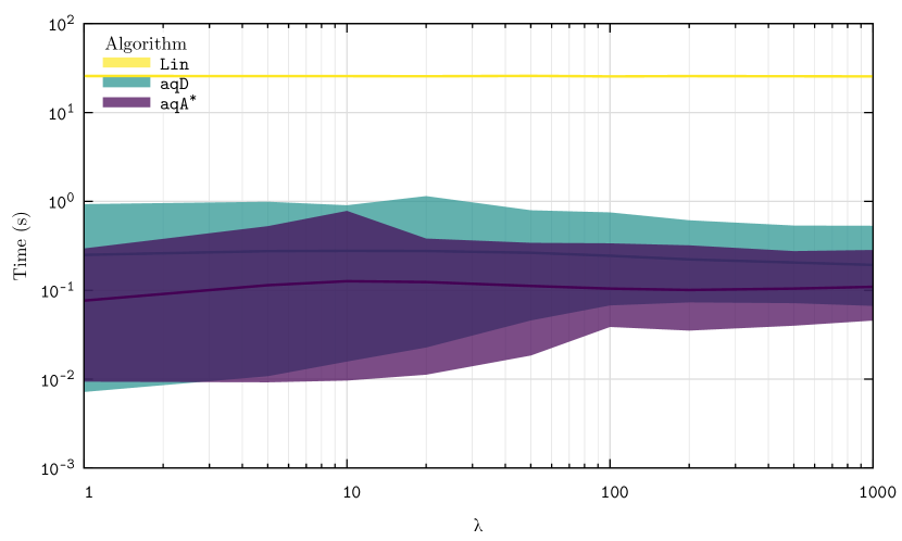
Figure 4: Results for Erdős-Rényi instances with $\lambda$ variation

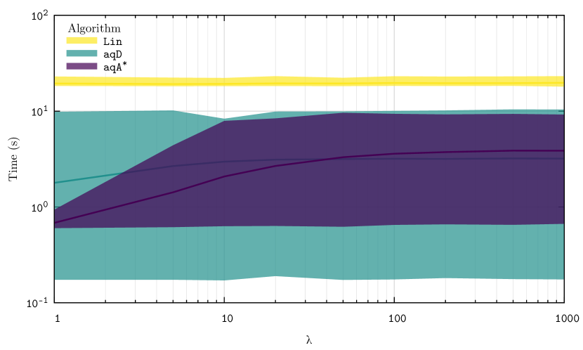
Figure 5: Results for Configuration Model instances with $\lambda$ variation

These results highlight the solution capability of aqA^* since it uses a cost-to-go estimator that we would expect to lose relevance as quadratic costs increase. Nevertheless, the $\lambda$ scale factors chosen for these experiments do not reverse the costs-to-go into a poor estimator. In other words, even with quadratic costs scaled up by a factor of $\lambda=1,000$, the estimator still provides valuable guidance for the search process. This behavior highlights the robustness of the proposed algorithm.

6.4 Grid Graphs

For the following experiments, we consider actual grid graph instances of spatial nature. Each node is associated with an actual location on the globe, and the arc costs represent the distances between locations. The graphs are built out of a regularly spaced grid of elevation points, which we define on (4) as the matrix $Y$ with $N$ rows and $M$ columns. Each element of the matrix is associated with a numeric value and spatial coordinates.

$$\centering Y=\begin{bmatrix}y_{11}&\dots&y_{1M}\\ \vdots&\ddots&\vdots\\ y_{N1}&\dots&y_{NM}\\ \end{bmatrix}\@add@centering$$ (4)

To create a graph instance, we convert the matrix $Y$ into a weighted graph, where each node $i\in V$ is equivalent to the element $y_{nm}$ with $|V|$ the product of matrix dimensions $N$×$M$, and $|A|$ can range according to a graph composition rule. This rule is a function of how many neighbors $n$ each node connects to. Figure 6 presents the effect of choosing different number of neighbors on $|A|$.

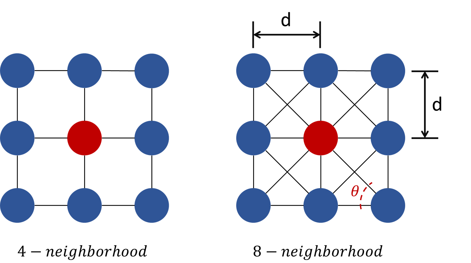
Figure 6: Illustration of node neighborhood for $n=8$ and $n=16$

The intuition behind node neighborhood comes from direction and length of movement. Common choices for $n$ are $\{2,4,8\}$. For instance, choosing $n=2$ or $n=4$ represent unitary movements on two directions (east and south) or on four directions (west/east and north/south), respectively. On the other hand, for $n=8$, diagonal movements are contemplated.

We denote by $d(y_{nm},y_{op})$ as a function that calculates the distance cost between points $y_{nm}$ and $y_{op}$. Thus, arc linear costs are defined as $\{c\big{(}(i,j)\big{)}=d(y_{nm},y_{op})\quad|\quad i=(n,m)\quad\text{and}\quad j=(o,p)\}$, where $(n,m)$ and $(o,p)$ are neighbors according to a given graph composition rule. For expository purposes, in this work, we set $n=8$ so that diagonal movements are allowed. As we are working with spatial information, diagonal costs must be adjusted by a factor of $\sqrt{2}$ following standard trigonometric developments. Figure 7 presents the results for all considered algorithms.

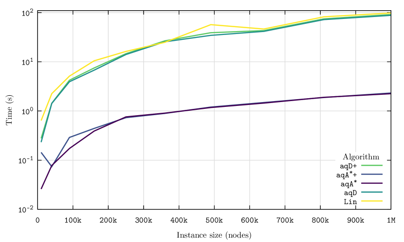
Figure 7: Grid Graphs: Search Time Comparison

Numerical results depicted in Figure 7 present the aqA^* as the fastest algorithm among all AQSPP algorithms considered. The aqA^* algorithm is approximately 39 times faster than aqD and roughly 53 times faster than Lin approach on average. Also, it seems the ratios fluctuate around this average value, which suggest a constant relation. A possible explanation for this over-performance is related to the similarity of paths obtained from SPP and AQSPP algorithms, resulting in exact cost-to-go estimators, thus speeding up aqA^*. Lin’s method, on the other hand, is outperformed by all the algorithms proposed in this work. The results displayed in Figure 7 show an aqD improvement in speed ranging between 10% up to a 50% in comparison to the Lin approach. Further analyses revealed that the time spent to linearize the graph is very significant and becomes a downside to the Lin approach, especially as instances grow in size. Figure 7 helps us notice the similarity between the original and modified versions of our algorithms, for both aqD and aqA^*. Although calculating the quadratic costs on the run lowers the search speed, the impact is negligible. Since the modified versions benefit from memory allocation reductions and allow solving larger instances, we highly recommend their use for applications where adaptation is a viable resource.

6.5 Stress test

We also provide a final experiment designed to stress search capabilities on extremely large-scale instances, ranging from $144\times 10^{6}$ to $10^{9}$ quadratic arcs. Since real applications may require path search on these instance sizes, evaluating the algorithms performance over increasingly larger graph instances can provide meaningful insights. Figure 8 displays the results from these experiments. It presents the search time for all approaches considered in this work using the extremely large-scale grid graph instances, generated following the same strategy as in Section 6.4.

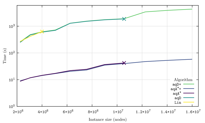
Figure 8: Stress Analysis: Search-Time Comparison

The results show that none of the original algorithms is able to solve all instances due to memory issues. Since the methods assume a preexisting structure that maps adjacent arcs into quadratic costs, storing this data become challenging as instances grow. Furthermore, aqD and aqA^* have internal data structures to store relevant information throughout the search process, which also requires memory space. The Lin approach presented an even higher demand for memory allocation since, by construction, there is a need to store the linearized graph. The marker on each approach in Figure 8 displays the maximum instance size each approach is able to solve. The large instance Lin is able to solve has $256\times 10^{6}$ quadratic nodes. On the other hand, aqD and aqA^* algorithms have similar extensions, solving instances up to $676\times 10^{6}$ quadratic nodes, but aqA^* algorithm obtains the same solution in $2.26\%$ of the aqD computing time. In contrast, the modified versions of aqD and aqA^* are able to solve all instances tested. Since quadratic calculations are made throughout the search, these algorithms do not require significant memory space, allowing them to handle increasingly larger instances properly. As expected, aqA^*+ remains the faster approach, solving the AQSPP in roughly 60.0 seconds on a graph with $16\times 10^{6}$ nodes, $64\times 10^{6}$ arcs and $10^{9}$ quadratic arcs, $1.34\%$ of the aqD+ computing time.

7 Conclusion

This study provides a theoretical description of Adjacent Quadratic Shortest Problems and proposes an extension of Dijkstra’s algorithm (aqD) to solve AQSPPs on graphs with no improving $\alpha$-cycles. Two enhancement procedures for the primary approach are also presented in this work: an adjacent quadratic version of A^* with backward cost-to-go estimation and an embedded calculation of adjacent quadratic costs. From the theoretical perspective, we present evidence that aqD can solve AQSPPs in polynomial time to proven optimality. We also show through computational experiments that aqD outperforms the algorithm proposed by Rostami et al. (2015), being more than 75$\times$ faster on very-large scale instances and a high scalability capability. This behavior is also valid for the proposed algorithm aqA^*, which was the fastest approach among the ones studied, outperforming aqD search speed by about the same amount on the benchmark analysis. Furthermore, other test results suggest that the proposed algorithms also had significant performance under randomly generated instances, indicating their robustness. In addition, we identified a significant drawback on Lin method (Rostami et al., 2015) for highly connected graphs related to the time spent performing the linearization step. Moreover, the algorithms were also indifferent to adjacent quadratic cost variation, already expected for aqD and an interesting result for aqA^*. Finally, results suggest that even for a high quadratic-linear cost ratio, the backward search is still profoundly relevant to enhance the aqA^* solution capability.

Future research shall focus on extending our findings to elementary variants of the AQSPP, relevant when the graph contains negative ($\alpha$-)cycles. This would be critical in quadratic variants of vehicle routing problems (Fischer and Helmberg, 2013; Martinelli and Contardo, 2015) when solved by column generation. Another interesting avenue for future research would be to extend our approach to the case where no negative ($\alpha$-)cycles exist, but where some (pairs of) arcs may be associated to negative costs. In this context, one shall develop label-correcting variants of our method in the spirit of Bellman (1958).

Appendix A Detailed Computational Results

In this section, we present the complete computational results obtained in the experiments of this paper.

A.1 Random Graphs

In Tables LABEL:tbl:erdos and LABEL:tbl:conf-model, we present the detailed results for the Erdős-Rényi and the Configuration Model random graphs. Both generation algorithms are tested for different random graph sizes, 100 graphs for each size. For each size and graph, we present the search time of Lin, aqD, and aqA^* approaches.

A.2 Quadratic Cost Variation

In Tables LABEL:tbl:lambda-erdos and LABEL:tbl:lambda-conf-model, we present the detailed results for the quadratic cost variation experiment using the Erdős-Rényi and the Configuration Model random graphs. Both generation algorithms are tested for different $\lambda$ values, 100 graphs for each value. For each value and graph, we present the search time of Lin, aqD, and aqA^* approaches.

A.3 Grid Graphs

Table 5 presents the detailed results for the grid graph instances. For each instance size, we present the search time for all tested approaches, including the modified versions of aqD and aqA^*.

A.4 Stress Test

Table 6 presents the detailed results for the stress test using the grid graph instances. For each instance size, we present the search time for all tested approaches, including the modified versions of aqD and aqA^*.

Inst	100 nodes				150 nodes				200 nodes				250 nodes				300 nodes				350 nodes				400 nodes
	Lin	aqD	aqA*		Lin	aqD	aqA*		Lin	aqD	aqA*		Lin	aqD	aqA*		Lin	aqD	aqA*		Lin	aqD	aqA*		Lin	aqD	aqA*
1	0.358	0.009	0.006		1.328	0.061	0.004		3.617	0.006	0.017		7.303	0.027	0.009		12.362	0.183	0.028		17.787	0.155	0.015		28.916	0.216	0.072
2	0.423	0.006	0.007		1.192	0.014	0.021		3.463	0.009	0.011		6.903	0.096	0.043		12.424	0.042	0.012		17.772	0.093	0.094		29.024	0.515	0.119
3	0.492	0.006	0.004		1.528	0.012	0.004		3.280	0.038	0.003		6.411	0.049	0.014		11.369	0.048	0.114		17.828	0.183	0.057		28.715	0.019	0.055
4	0.399	0.011	0.001		1.353	0.031	0.007		3.191	0.008	0.017		6.746	0.117	0.070		11.325	0.076	0.047		17.968	0.197	0.028		29.059	0.481	0.114
5	0.427	0.009	0.008		1.380	0.013	0.008		3.282	0.050	0.003		6.985	0.102	0.065		11.126	0.293	0.026		17.683	0.206	0.032		28.808	0.197	0.530
6	0.392	0.026	0.007		1.366	0.036	0.002		3.393	0.046	0.031		6.577	0.135	0.066		11.156	0.052	0.037		17.822	0.074	0.016		29.351	0.596	0.016
7	0.371	0.016	0.006		1.369	0.012	0.008		3.295	0.027	0.022		6.490	0.088	0.012		11.327	0.075	0.030		17.699	0.060	0.058		29.396	0.073	0.028
8	0.414	0.007	0.005		1.356	0.013	0.004		3.195	0.004	0.003		6.370	0.028	0.061		11.355	0.209	0.110		17.933	0.072	0.022		28.795	0.392	0.398
9	0.490	0.035	0.001		1.355	0.005	0.010		3.657	0.030	0.013		6.320	0.133	0.061		11.102	0.154	0.132		17.842	0.169	0.057		29.217	0.141	0.294
10	0.399	0.010	0.008		1.350	0.025	0.002		3.194	0.018	0.038		6.231	0.101	0.069		11.080	0.103	0.030		17.959	0.044	0.020		28.841	0.341	0.170
11	0.426	0.015	0.011		1.350	0.014	0.011		3.484	0.166	0.043		6.259	0.082	0.088		11.432	0.110	0.036		17.959	0.135	0.137		29.083	0.500	0.166
12	0.394	0.019	0.006		1.333	0.012	0.004		3.247	0.057	0.007		6.099	0.075	0.021		11.298	0.229	0.007		17.867	0.048	0.237		28.862	0.071	0.132
13	0.352	0.002	0.005		1.349	0.007	0.001		3.236	0.001	0.012		6.208	0.150	0.074		13.499	0.055	0.017		17.792	0.030	0.017		29.043	0.249	0.115
14	0.424	0.002	0.001		1.355	0.001	0.002		3.221	0.012	0.003		6.610	0.231	0.086		12.112	0.145	0.060		18.016	0.057	0.050		29.180	0.493	0.162
15	0.494	0.024	0.004		1.338	0.013	0.006		3.263	0.073	0.006		6.185	0.084	0.170		11.556	0.159	0.009		17.866	0.009	0.014		29.338	0.666	0.061
16	0.402	0.013	0.009		1.332	0.016	0.013		3.259	0.046	0.011		6.146	0.090	0.031		11.199	0.064	0.038		17.823	0.066	0.045		28.941	0.106	0.314
17	0.427	0.035	0.003		1.351	0.044	0.005		3.337	0.048	0.011		6.341	0.047	0.022		11.507	0.047	0.022		17.777	0.056	0.036		29.289	0.136	0.043
18	0.400	0.012	0.006		1.339	0.050	0.012		3.218	0.004	0.014		6.261	0.150	0.025		11.180	0.010	0.078		18.014	0.396	0.106		29.471	0.110	0.259
19	0.357	0.010	0.002		1.346	0.025	0.004		3.291	0.019	0.023		6.013	0.470	0.036		11.626	0.343	0.049		17.772	0.021	0.178		29.028	0.407	0.134
20	0.419	0.027	0.008		1.352	0.018	0.005		3.203	0.074	0.019		6.363	0.051	0.055		11.294	0.035	0.020		18.045	0.165	0.042		29.480	0.199	0.144
21	0.499	0.006	0.009		1.343	0.029	0.004		3.192	0.075	0.022		6.144	0.073	0.039		11.106	0.039	0.033		17.804	0.042	0.049		29.293	0.025	0.066
22	0.404	0.014	0.003		1.328	0.013	0.009		3.255	0.011	0.034		6.367	0.083	0.022		11.444	0.294	0.019		17.873	0.081	0.082		29.030	0.230	0.095
23	0.441	0.009	0.014		1.352	0.012	0.002		3.340	0.070	0.025		6.293	0.021	0.037		11.514	0.007	0.096		17.809	0.095	0.081		29.849	0.256	0.437
24	0.420	0.016	0.002		1.350	0.009	0.009		3.237	0.106	0.013		6.394	0.050	0.043		12.261	0.221	0.031		17.905	0.142	0.033		29.327	0.459	0.118
25	0.349	0.042	0.007		1.342	0.002	0.036		3.281	0.006	0.002		7.060	0.087	0.011		12.869	0.005	0.015		17.750	0.174	0.028		29.079	0.547	0.098
26	0.421	0.010	0.010		1.336	0.016	0.018		3.307	0.046	0.010		7.497	0.044	0.088		11.666	0.081	0.017		17.959	0.014	0.012		29.017	0.142	0.179
27	0.490	0.019	0.007		1.341	0.008	0.011		3.244	0.040	0.015		6.721	0.163	0.063		11.219	0.088	0.083		18.025	0.102	0.025		28.912	0.835	0.045
28	0.402	0.020	0.003		1.333	0.010	0.015		3.219	0.004	0.004		6.184	0.074	0.017		11.219	0.036	0.164		18.055	0.126	0.028		29.338	0.058	0.162
29	0.440	0.005	0.001		1.356	0.034	0.013		3.328	0.091	0.008		6.709	0.079	0.031		11.317	0.322	0.015		17.936	0.061	0.128		28.859	0.081	0.099
30	0.454	0.033	0.002		1.339	0.107	0.003		3.223	0.066	0.024		6.238	0.067	0.057		11.310	0.081	0.031		18.134	0.051	0.013		29.006	0.070	0.220
31	0.351	0.010	0.007		1.348	0.027	0.001		3.195	0.023	0.019		6.374	0.039	0.067		11.328	0.155	0.036		18.134	0.220	0.077		29.167	0.224	0.092
32	0.418	0.002	0.002		1.343	0.007	0.016		3.207	0.012	0.012		6.235	0.061	0.020		11.243	0.134	0.020		17.807	0.153	0.090		29.518	0.182	0.088
33	0.491	0.002	0.002		1.353	0.007	0.003		3.143	0.078	0.004		6.213	0.033	0.010		10.855	0.162	0.098		17.786	0.130	0.056		29.469	0.311	0.178
34	0.397	0.006	0.003		1.355	0.005	0.004		3.251	0.006	0.003		6.216	0.047	0.031		11.382	0.045	0.038		17.808	0.388	0.010		28.913	0.434	0.019
35	0.427	0.008	0.004		1.399	0.001	0.013		3.288	0.040	0.002		6.181	0.017	0.057		11.414	0.051	0.038		17.964	0.232	0.163		28.990	0.234	0.083
36	0.404	0.014	0.001		1.383	0.020	0.002		3.182	0.007	0.033		6.259	0.051	0.015		11.285	0.008	0.007		17.976	0.013	0.075		29.137	0.597	0.120
37	0.353	0.002	0.006		1.373	0.036	0.016		3.202	0.011	0.004		6.457	0.124	0.069		12.847	0.025	0.080		17.760	0.016	0.024		29.428	0.147	0.035
38	0.420	0.017	0.017		1.496	0.047	0.033		3.193	0.004	0.007		6.265	0.075	0.016		11.681	0.075	0.008		17.757	0.015	0.037		29.227	0.087	0.040
39	0.497	0.019	0.004		1.341	0.047	0.012		3.244	0.029	0.005		6.073	0.168	0.078		11.240	0.084	0.087		17.721	0.232	0.026		29.129	0.274	0.017
40	0.399	0.006	0.005		1.348	0.026	0.007		3.306	0.031	0.023		6.341	0.032	0.028		11.267	0.021	0.018		17.883	0.060	0.035		28.879	0.136	0.116
41	0.428	0.019	0.001		1.362	0.004	0.017		3.280	0.020	0.027		6.281	0.057	0.020		11.253	0.059	0.021		17.944	0.091	0.076		28.918	0.036	0.068
42	0.394	0.008	0.005		1.350	0.024	0.011		3.321	0.027	0.003		6.099	0.029	0.031		11.026	0.011	0.079		17.864	0.127	0.014		28.914	0.162	0.054
43	0.358	0.012	0.004		1.331	0.037	0.022		3.208	0.024	0.021		6.404	0.047	0.054		11.404	0.112	0.054		17.771	0.158	0.033		28.850	0.202	0.046
44	0.429	0.006	0.002		1.350	0.015	0.008		3.209	0.012	0.018		6.273	0.146	0.018		11.426	0.048	0.072		18.094	0.152	0.009		29.297	0.069	0.129
45	0.509	0.006	0.007		1.347	0.005	0.001		3.168	0.016	0.002		6.463	0.038	0.065		11.127	0.115	0.104		17.918	0.045	0.137		29.075	0.123	0.066
46	0.394	0.005	0.005		1.362	0.011	0.002		3.315	0.026	0.009		6.214	0.137	0.018		11.315	0.298	0.024		17.788	0.242	0.063		29.031	0.066	0.313
47	0.440	0.005	0.011		1.359	0.004	0.008		3.759	0.071	0.004		6.374	0.034	0.040		11.419	0.010	0.023		17.812	0.049	0.353		29.255	0.065	0.118
48	0.396	0.014	0.004		1.339	0.004	0.010		3.594	0.018	0.028		7.714	0.015	0.063		12.188	0.059	0.054		18.038	0.073	0.020		28.939	0.484	0.043
49	0.360	0.015	0.001		1.337	0.024	0.010		3.605	0.166	0.020		7.019	0.154	0.021		12.225	0.004	0.045		17.736	0.466	0.011		28.888	0.296	0.057
50	0.425	0.009	0.002		1.403	0.002	0.013		3.535	0.085	0.006		6.514	0.230	0.082		11.882	0.009	0.024		17.843	0.191	0.019		29.107	0.131	0.191
51	0.491	0.019	0.006		1.338	0.003	0.009		3.311	0.056	0.009		6.417	0.032	0.036		11.336	0.085	0.066		17.738	0.038	0.044		28.921	0.515	0.079
52	0.412	0.009	0.007		1.358	0.008	0.009		3.280	0.013	0.044		7.316	0.142	0.072		11.116	0.048	0.043		17.837	0.046	0.051		29.166	0.250	0.092
53	0.423	0.015	0.002		1.361	0.036	0.010		3.308	0.030	0.053		9.390	0.335	0.012		11.246	0.250	0.048		17.850	0.013	0.089		29.150	0.034	0.123
54	0.384	0.007	0.004		1.359	0.012	0.016		3.379	0.006	0.010		6.588	0.019	0.051		11.374	0.019	0.043		17.791	0.090	0.076		28.812	0.044	0.053
55	0.346	0.005	0.001		1.354	0.022	0.005		3.458	0.025	0.009		6.896	0.133	0.011		11.367	0.045	0.018		18.100	0.037	0.055		28.910	0.163	0.013
56	0.408	0.002	0.008		1.383	0.024	0.003		3.214	0.054	0.011		10.833	0.033	0.035		11.258	0.145	0.034		17.955	0.022	0.010		29.255	0.012	0.035
57	0.483	0.009	0.002		1.339	0.022	0.001		3.349	0.010	0.025		11.947	0.068	0.045		10.899	0.209	0.032		18.220	0.355	0.046		29.025	0.038	0.078
58	0.385	0.006	0.005		1.326	0.023	0.004		3.276	0.013	0.015		12.384	0.111	0.015		11.378	0.050	0.106		17.808	0.177	0.069		28.844	0.179	0.019
59	0.420	0.003	0.005		1.331	0.010	0.009		3.593	0.046	0.012		12.074	0.292	0.087		11.554	0.123	0.044		17.831	0.127	0.127		28.939	0.092	0.065
60	0.385	0.002	0.003		1.325	0.003	0.012		3.399	0.024	0.043		7.520	0.051	0.024		12.443	0.072	0.043		17.763	0.154	0.025		28.865	0.109	0.052
61	0.350	0.008	0.004		1.330	0.013	0.004		3.303	0.011	0.015		6.233	0.093	0.018		12.219	0.174	0.034		17.766	0.059	0.105		29.203	0.273	0.105
62	0.413	0.007	0.003		1.367	0.034	0.014		3.474	0.006	0.014		6.214	0.156	0.067		11.431	0.075	0.025		17.784	0.218	0.211		28.743	0.468	0.243
63	0.485	0.002	0.006		1.335	0.026	0.004		3.201	0.007	0.010		6.225	0.054	0.080		11.046	0.117	0.009		17.761	0.339	0.053		28.956	0.269	0.064
64	0.386	0.012	0.011		1.348	0.017	0.002		3.278	0.011	0.009		6.163	0.083	0.021		11.270	0.020	0.018		17.835	0.272	0.119		28.931	0.080	0.122
65	0.427	0.007	0.007		1.354	0.018	0.004		3.358	0.085	0.005		6.271	0.052	0.062		11.164	0.051	0.055		17.763	0.115	0.058		29.286	0.038	0.175
66	0.384	0.008	0.010		1.363	0.043	0.004		3.216	0.016	0.014		6.532	0.038	0.021		11.254	0.010	0.007		17.764	0.127	0.009		28.845	0.165	0.048
67	0.339	0.029	0.006		1.357	0.008	0.018		3.222	0.016	0.023		6.434	0.059	0.036		11.133	0.235	0.140		17.727	0.033	0.010		29.790	0.198	0.028
68	0.405	0.004	0.006		1.361	0.013	0.004		3.140	0.076	0.012		6.352	0.133	0.013		11.205	0.043	0.030		18.170	0.021	0.016		29.360	0.304	0.061
69	0.482	0.011	0.007		1.359	0.020	0.011		3.168	0.023	0.003		6.268	0.059	0.067		11.269	0.055	0.070		17.781	0.248	0.151		28.595	0.066	0.055
70	0.395	0.018	0.003		1.376	0.025	0.019		3.207	0.012	0.029		6.277	0.042	0.055		11.363	0.156	0.211		17.949	0.022	0.022		28.772	0.045	0.034
71	0.420	0.003	0.005		1.344	0.001	0.007		3.307	0.005	0.006		6.273	0.289	0.041		11.566	0.138	0.030		17.930	0.037	0.024		28.705	0.271	0.094
72	0.397	0.012	0.005		1.365	0.012	0.005		3.218	0.016	0.030		6.402	0.122	0.014		13.167	0.097	0.008		17.729	0.109	0.022		28.323	0.288	0.093
73	0.352	0.005	0.005		1.384	0.011	0.006		3.170	0.007	0.014		6.217	0.062	0.023		11.929	0.048	0.020		17.685	0.276	0.024		28.331	0.253	0.034
74	0.428	0.007	0.013		1.414	0.045	0.007		3.227	0.018	0.019		6.435	0.077	0.023		11.594	0.185	0.088		18.007	0.053	0.021		28.472	0.099	0.015
75	0.496	0.012	0.005		1.340	0.004	0.010		3.141	0.018	0.003		6.323	0.184	0.057		11.021	0.021	0.074		17.866	0.056	0.024		28.225	0.105	0.050
76	0.410	0.013	0.008		1.370	0.012	0.005		3.238	0.073	0.009		6.462	0.123	0.049		11.210	0.012	0.069		17.986	0.124	0.050		28.340	0.102	0.319
77	0.415	0.006	0.008		1.350	0.045	0.002		3.376	0.015	0.017		7.885	0.057	0.058		11.374	0.011	0.058		17.830	0.245	0.012		28.649	0.185	0.184
78	0.389	0.008	0.004		1.367	0.025	0.007		3.395	0.006	0.004		6.948	0.254	0.021		11.212	0.022	0.009		18.078	0.012	0.019		28.842	0.237	0.062
79	0.343	0.006	0.004		1.349	0.001	0.002		3.226	0.108	0.004		6.427	0.048	0.045		11.428	0.129	0.039		17.639	0.032	0.019		28.289	0.219	0.232
80	0.423	0.011	0.006		1.345	0.028	0.002		3.172	0.005	0.005		6.683	0.027	0.011		11.053	0.093	0.078		18.091	0.199	0.012		28.809	0.167	0.025
81	0.512	0.005	0.009		1.372	0.021	0.010		3.171	0.003	0.002		6.456	0.076	0.015		11.276	0.045	0.029		17.740	0.174	0.069		28.537	0.890	0.020
82	0.404	0.006	0.006		1.354	0.009	0.004		3.221	0.033	0.022		6.262	0.055	0.014		11.426	0.182	0.043		17.983	0.051	0.047		28.342	0.070	0.130
83	0.439	0.006	0.005		1.360	0.014	0.028		3.387	0.033	0.012		7.690	0.069	0.008		11.643	0.116	0.088		17.717	0.032	0.052		28.436	0.073	0.035
84	0.394	0.008	0.003		1.400	0.002	0.002		3.199	0.017	0.005		9.655	0.024	0.077		12.344	0.053	0.006		17.777	0.100	0.029		28.492	0.252	0.096
85	0.356	0.006	0.005		1.354	0.028	0.001		3.229	0.003	0.010		6.605	0.057	0.068		11.448	0.295	0.022		17.872	0.127	0.048		28.663	1.273	0.152
86	0.437	0.004	0.003		1.378	0.028	0.009		3.109	0.010	0.011		8.897	0.063	0.044		10.798	0.092	0.087		17.858	0.452	0.091		28.323	0.043	0.073
87	0.500	0.007	0.005		1.371	0.026	0.012		3.101	0.075	0.003		9.432	0.057	0.006		10.570	0.055	0.053		17.759	0.048	0.038		28.677	0.131	0.075
88	0.438	0.014	0.012		1.356	0.022	0.015		3.245	0.007	0.007		10.383	0.049	0.048		10.673	0.326	0.142		17.825	0.086	0.062		28.591	0.500	0.038
89	0.435	0.030	0.004		1.726	0.011	0.007		3.327	0.020	0.010		10.291	0.210	0.038		10.816	0.071	0.045		17.750	0.143	0.011		29.112	0.284	0.073
90	0.393	0.016	0.002		1.535	0.028	0.005		3.289	0.004	0.006		9.683	0.065	0.028		10.650	0.071	0.028		18.050	0.011	0.042		28.362	0.254	0.234
91	0.363	0.006	0.012		1.452	0.005	0.011		3.259	0.003	0.012		9.138	0.081	0.034		10.824	0.125	0.025		17.684	0.093	0.019		28.787	0.111	0.064
92	0.423	0.013	0.005		1.895	0.003	0.010		3.182	0.035	0.013		7.587	0.102	0.016		10.814	0.037	0.009		17.848	0.403	0.016		28.667	0.568	0.248
93	0.521	0.005	0.001		1.505	0.006	0.003		3.226	0.033	0.006		10.120	0.185	0.012		10.689	0.045	0.022		18.078	0.208	0.015		28.407	0.030	0.114
94	0.396	0.022	0.005		1.485	0.011	0.005		3.257	0.025	0.045		6.821	0.048	0.009		10.767	0.013	0.020		17.975	0.092	0.013		28.339	0.232	0.094
95	0.450	0.013	0.002		1.467	0.004	0.021		3.310	0.067	0.003		7.057	0.068	0.232		10.848	0.039	0.007		17.822	0.189	0.103		28.328	0.199	0.198
96	0.396	0.019	0.011		1.552	0.003	0.009		3.225	0.020	0.009		7.210	0.072	0.033		10.585	0.084	0.011		17.945	0.092	0.071		28.747	0.297	0.013
97	0.356	0.012	0.008		1.456	0.004	0.004		3.272	0.038	0.009		7.545	0.089	0.018		10.727	0.012	0.201		17.776	0.322	0.034		28.810	0.259	0.017
99	0.497	0.013	0.003		1.387	0.013	0.019		3.880	0.063	0.027		7.597	0.153	0.083		10.725	0.010	0.005		17.807	0.013	0.037		28.326	0.635	0.096
100	0.414	0.005	0.010		1.386	0.010	0.003		3.878	0.053	0.013		7.358	0.247	0.033		11.008	0.327	0.109		17.882	0.083	0.035		28.404	0.371	0.127
Avg	0.417	0.011	0.005		1.376	0.018	0.009		3.298	0.033	0.014		7.060	0.096	0.043		11.393	0.098	0.049		17.870	0.127	0.056		28.920	0.248	0.115

Table 1: Results for Erdős-Rényi random graphs

Inst	100k nodes				150k nodes				200k nodes				250k nodes				300k nodes
	Lin	aqD	aqA*		Lin	aqD	aqA*		Lin	aqD	aqA*		Lin	aqD	aqA*		Lin	aqD	aqA*
1	6.100	2.616	0.204		10.843	3.267	0.298		12.860	5.341	0.467		15.809	6.519	0.502		23.250	1.590	0.684
2	6.185	3.263	0.196		10.870	1.599	0.264		14.650	1.054	0.426		17.455	2.198	0.510		21.749	5.020	0.641
3	6.593	0.760	0.207		10.867	2.189	0.270		12.942	1.150	0.388		17.602	0.383	0.551		19.976	5.823	0.734
4	6.852	2.607	0.181		10.638	3.254	0.316		13.344	0.854	0.406		16.182	1.159	0.537		21.656	0.828	0.629
5	6.501	0.660	0.247		12.308	0.885	0.262		14.079	1.721	0.449		16.111	6.560	0.504		24.461	1.194	0.673
6	6.619	0.294	0.172		11.375	1.280	0.266		12.710	5.231	0.441		16.725	0.884	0.530		22.030	1.588	0.635
7	6.658	2.569	0.221		11.712	3.994	0.257		12.985	2.069	0.426		16.803	1.680	0.592		22.364	3.337	0.627
8	7.000	2.955	0.157		11.590	1.900	0.358		13.603	4.593	0.394		15.565	3.262	0.514		23.157	7.552	0.613
9	6.910	1.120	0.154		11.501	3.271	0.293		13.007	6.147	0.449		15.874	3.104	0.714		22.571	7.289	0.693
10	7.192	0.878	0.312		11.282	3.056	0.259		14.432	1.669	0.385		17.524	0.220	0.570		20.579	0.225	0.619
11	7.090	0.635	0.167		10.378	2.109	0.277		14.133	0.475	0.388		18.220	1.430	0.515		22.740	5.103	0.608
12	6.785	0.895	0.205		11.275	3.689	0.260		14.423	3.454	0.420		17.512	2.274	0.534		21.329	1.039	0.690
13	6.395	0.833	0.195		11.087	3.802	0.278		13.617	0.483	0.435		15.674	2.309	0.500		21.212	4.161	0.716
14	6.398	2.072	0.479		10.900	2.585	0.258		13.713	2.462	0.397		16.304	0.394	0.566		20.966	3.604	0.656
15	5.981	2.777	0.214		11.509	0.863	0.255		13.718	3.249	0.420		15.893	3.646	0.524		19.805	4.400	0.639
16	7.244	2.757	0.163		9.974	1.255	0.300		12.921	0.854	0.426		17.513	2.919	0.550		19.195	1.088	0.619
17	6.598	2.653	0.232		10.898	1.389	0.256		14.656	3.158	0.409		15.662	1.938	0.563		22.211	7.916	0.720
18	6.683	1.782	0.179		10.991	1.157	0.318		13.541	0.243	0.375		15.641	3.226	0.524		22.175	2.778	0.628
19	6.297	1.467	0.189		10.516	2.972	0.310		13.023	1.549	0.415		16.073	5.277	0.630		20.483	3.367	0.626
20	6.674	0.508	0.236		10.110	2.968	0.283		14.534	0.194	0.456		17.556	6.711	0.559		23.063	4.559	0.682
21	6.878	1.102	0.156		11.624	2.641	0.258		12.758	2.341	0.402		19.123	1.991	0.509		20.292	3.971	0.720
22	6.403	1.219	0.196		10.569	1.317	0.282		14.177	0.309	0.404		15.642	4.939	0.546		23.188	0.217	0.702
23	6.576	2.326	0.185		9.965	1.503	0.285		13.746	4.972	0.428		17.661	2.365	0.527		21.415	4.158	0.623
24	6.317	1.554	0.179		11.128	2.665	0.370		13.051	0.346	0.394		17.942	1.099	0.524		20.614	3.051	0.698
25	7.104	2.866	0.150		9.539	0.578	0.285		12.767	2.576	0.417		16.021	4.254	0.511		22.624	1.658	0.655
26	7.094	1.584	0.311		10.259	0.366	0.275		13.500	1.239	0.403		17.842	0.613	0.552		20.962	1.933	0.697
27	6.933	1.570	0.235		9.863	2.928	0.278		12.681	0.890	0.399		17.456	7.691	0.500		21.206	3.500	0.704
28	7.023	1.050	0.164		11.125	2.823	0.334		12.875	0.401	0.418		16.290	2.383	0.489		21.938	3.090	0.617
29	7.111	0.299	0.275		9.392	3.505	0.297		13.389	1.598	0.449		15.997	2.604	0.494		22.049	9.378	0.661
30	6.310	1.659	0.273		10.817	5.053	0.260		12.789	0.715	0.394		17.799	6.165	0.504		20.999	4.338	0.681
31	6.668	0.236	0.184		11.393	2.649	0.268		13.545	1.460	0.434		17.163	0.312	0.531		23.155	5.577	0.622
32	7.208	0.791	0.193		10.460	2.411	0.308		13.845	2.885	0.376		19.176	0.928	0.519		22.734	8.751	0.852
33	6.543	2.598	0.255		11.066	1.089	0.343		13.739	2.829	0.410		16.983	3.399	0.623		20.868	3.389	0.648
34	6.348	1.930	0.267		10.462	2.295	0.263		12.923	4.646	0.415		16.310	1.331	0.634		23.226	3.118	0.653
35	6.282	1.157	0.180		10.195	1.237	0.296		12.793	2.110	0.449		17.249	1.054	0.515		23.872	2.390	0.643
36	7.259	2.414	0.154		10.419	2.864	0.282		13.173	3.216	0.389		17.032	0.732	0.512		22.406	4.462	0.684
37	6.503	3.050	0.234		10.136	1.479	0.280		15.081	2.086	0.421		17.340	6.021	0.538		20.675	1.917	0.649
38	7.006	1.611	0.184		9.872	1.312	0.273		14.129	1.711	0.390		16.145	2.048	0.548		24.631	0.989	0.723
39	6.246	1.221	0.160		10.118	1.661	0.262		13.267	1.173	0.398		19.142	1.696	0.549		20.639	3.808	0.694
40	6.272	2.831	0.189		9.889	1.306	0.478		12.864	3.449	0.428		18.503	2.912	0.544		23.443	1.066	0.613
41	7.065	1.076	0.180		9.736	3.826	0.262		12.641	4.013	0.402		16.536	5.317	0.503		23.316	8.270	0.661
42	6.079	1.546	0.218		9.450	2.138	0.306		12.813	0.840	0.395		17.000	3.347	0.582		21.803	7.119	0.646
43	6.624	1.038	0.205		9.924	2.277	0.262		13.287	5.332	0.477		18.013	0.702	0.621		21.428	6.204	0.618
44	6.804	1.344	0.173		9.980	0.383	0.268		13.340	0.839	0.407		16.305	1.217	0.480		23.139	1.537	0.674
45	6.965	1.819	0.275		11.107	2.496	0.261		13.010	2.453	0.402		15.850	0.659	0.507		21.497	6.423	0.674
46	6.424	1.589	0.241		9.905	2.907	0.258		14.473	3.651	0.386		16.198	4.799	0.529		22.129	1.330	0.683
47	5.970	2.176	0.181		10.027	0.668	0.258		13.549	0.345	0.419		15.579	1.498	0.615		21.693	3.176	0.648
48	6.522	1.895	0.149		9.805	2.776	0.260		13.057	3.522	0.415		16.278	4.272	0.601		21.419	7.971	0.662
49	6.416	0.690	0.163		9.423	1.438	0.281		14.506	0.685	0.421		16.005	1.441	0.502		20.919	7.932	0.637
50	6.121	2.066	0.147		9.985	1.939	0.265		12.931	2.209	0.391		18.100	6.394	0.544		24.394	3.679	0.894
51	6.959	1.066	0.182		10.344	5.078	0.303		14.017	1.812	0.419		15.464	2.979	0.502		21.194	3.944	0.678
52	6.742	1.467	0.174		10.467	0.254	0.325		12.647	3.515	0.419		16.130	3.013	0.513		21.086	0.771	0.628
53	7.371	2.541	0.173		11.177	5.336	0.265		15.160	4.022	0.452		16.018	0.792	0.617		20.780	8.585	0.643
54	6.341	0.715	0.254		9.779	2.134	0.455		12.871	0.690	0.401		17.650	0.917	0.504		20.539	6.371	0.690
55	7.198	0.425	0.231		10.286	4.536	0.293		12.846	3.619	0.429		15.494	0.859	0.515		19.653	4.815	0.607
56	6.126	2.421	0.185		10.706	3.310	0.254		12.720	1.297	0.372		16.126	1.933	0.578		22.426	7.166	0.727
57	6.434	2.825	0.181		9.985	0.378	0.313		13.583	5.205	0.423		17.233	0.345	0.554		25.044	8.031	0.631
58	7.010	0.380	0.165		9.867	4.597	0.260		15.870	0.590	0.383		19.243	6.452	0.826		22.893	9.506	0.660
59	6.489	2.107	0.151		9.870	3.123	0.279		12.707	2.365	0.413		17.814	5.816	0.614		21.531	7.346	0.628
60	6.828	2.228	0.180		9.656	4.656	0.359		13.878	3.566	0.399		16.569	7.096	0.509		21.064	3.274	0.645
61	6.632	2.279	0.171		10.847	1.456	0.390		13.566	3.140	0.515		17.929	1.508	0.563		21.355	3.801	0.850
62	6.202	2.069	0.164		11.141	4.704	0.402		14.296	0.504	0.397		18.100	3.476	0.527		20.085	4.910	1.169
63	7.025	0.437	0.242		10.267	1.352	0.281		13.370	2.249	0.421		17.072	5.888	0.557		21.193	4.065	0.607
64	6.340	0.548	0.150		10.874	2.057	0.301		14.143	2.366	0.384		15.450	3.221	0.802		21.114	8.288	0.656
65	6.649	1.747	0.235		10.450	2.434	0.279		13.207	6.685	0.452		15.369	0.558	0.497		20.214	2.956	0.724
66	6.439	1.336	0.161		9.294	1.988	0.248		13.496	0.838	0.416		16.136	2.147	0.557		21.580	2.744	0.641
67	6.637	1.351	0.160		10.325	1.539	0.288		12.823	1.553	0.422		16.734	6.529	0.560		22.779	3.018	0.625
68	6.989	1.415	0.147		11.298	2.475	0.265		14.296	0.718	0.401		15.838	3.820	0.659		20.370	2.431	0.669
69	6.092	0.968	0.201		9.304	2.784	0.306		12.858	4.746	0.438		15.387	7.566	0.536		23.534	4.291	0.718
70	6.489	2.424	0.172		10.218	1.708	0.295		14.562	4.905	0.399		16.051	0.480	0.531		20.428	3.383	0.628
71	6.231	0.917	0.156		10.930	2.449	0.281		13.323	3.930	0.405		17.666	2.098	0.510		20.052	2.984	0.644
72	7.060	2.174	0.247		9.734	1.368	0.247		13.878	3.893	0.377		16.923	9.159	0.635		24.489	11.020	0.812
73	6.904	1.857	0.162		10.155	3.271	0.266		14.053	2.300	0.418		17.099	3.459	0.588		21.761	6.274	0.646
74	6.976	0.824	0.198		9.528	1.753	0.266		13.602	3.759	0.412		15.545	1.594	0.536		22.525	0.346	0.659
75	7.183	0.717	0.148		10.218	3.184	0.266		13.362	1.264	0.393		16.150	0.687	0.563		21.538	5.115	0.689
76	6.648	0.832	0.216		9.571	3.912	0.290		13.332	1.602	0.405		16.145	1.995	0.491		19.800	1.780	0.639
77	6.369	1.054	0.204		10.463	4.356	0.310		12.970	0.560	0.490		16.319	1.679	0.522		20.946	1.796	0.685
78	6.742	0.770	0.166		9.889	3.230	0.313		12.900	2.217	0.386		15.651	3.909	0.615		23.106	1.237	0.626
79	6.994	1.917	0.189		11.017	4.253	0.329		12.927	0.194	0.405		15.513	2.393	0.509		23.693	2.502	0.688
80	5.981	0.698	0.191		10.002	2.888	0.266		13.309	1.065	0.446		16.203	2.754	0.501		20.110	6.993	0.635
81	7.022	2.667	0.233		10.105	3.264	0.279		13.462	2.739	0.428		17.718	1.685	0.692		21.466	3.328	0.653
82	7.026	2.214	0.165		11.318	2.793	0.267		13.198	5.212	0.374		16.806	2.790	0.557		19.677	9.951	0.688
83	6.920	1.579	0.151		9.906	2.861	0.290		14.650	0.654	0.392		17.759	1.421	0.548		20.471	8.855	0.618
84	6.853	2.444	0.236		9.754	4.709	0.257		15.449	2.265	0.431		16.019	0.413	0.505		20.998	4.289	0.758
85	6.838	1.448	0.156		9.653	1.874	0.272		13.550	0.709	0.421		17.126	1.095	0.544		20.759	3.925	0.632
86	6.829	2.409	0.180		10.260	1.454	0.271		13.147	1.116	0.470		17.199	1.678	0.544		22.661	4.055	0.686
87	7.086	2.945	0.180		11.667	0.470	0.269		13.302	1.559	0.412		16.049	8.095	0.629		22.556	4.578	0.728
88	6.398	2.401	0.188		9.524	0.328	0.270		13.883	1.144	0.381		16.337	4.184	0.588		20.721	4.166	0.651
89	6.847	0.576	0.148		11.000	3.219	0.251		12.935	3.953	0.467		15.742	0.612	0.538		20.410	3.777	0.672
90	6.979	0.704	0.203		10.142	3.467	0.296		14.866	1.748	0.399		16.964	5.564	0.512		21.201	1.261	0.759
91	6.598	2.349	0.184		10.567	0.210	0.320		13.584	1.078	0.432		15.716	2.061	0.592		22.582	4.261	0.666
92	7.143	1.073	0.175		9.493	0.595	0.278		13.295	1.652	0.402		15.565	1.054	0.506		22.761	2.998	0.638
93	6.507	2.085	0.244		11.228	0.460	0.313		13.127	2.589	0.394		15.441	1.621	0.505		19.946	4.426	0.641
94	6.952	1.803	0.189		10.834	2.644	0.295		14.155	2.502	0.436		16.305	2.185	0.516		21.146	0.697	0.767
95	5.907	1.700	0.164		10.726	3.260	0.278		12.855	1.993	0.455		18.222	0.920	0.551		22.912	1.360	0.814
96	6.016	0.988	0.150		10.408	1.633	0.321		12.654	1.433	0.371		15.841	2.805	0.630		22.969	1.938	0.638
97	6.049	2.784	0.152		10.303	2.426	0.272		13.308	2.287	0.453		17.416	3.419	0.549		19.846	2.708	0.678
98	6.194	2.839	0.178		9.728	1.159	0.293		12.828	3.081	0.399		18.448	3.844	0.651		20.618	6.130	0.654
99	6.793	1.668	0.286		10.058	0.154	0.264		12.670	1.744	0.395		16.639	3.320	0.578		20.431	7.359	0.653
100	5.839	2.502	0.161		11.217	2.811	0.287		13.096	0.404	0.402		15.613	1.530	0.502		21.967	1.773	0.810
Avg	6.647	1.641	0.196		10.438	2.364	0.289		13.502	2.258	0.415		16.723	2.857	0.554		21.706	4.184	0.678

Table 2: Results for Configuration Model random graphs

Inst	$\lambda=1$				$\lambda=5$				$\lambda=50$				$\lambda=500$				$\lambda=1000$
	Lin	aqD	aqA*		Lin	aqD	aqA*		Lin	aqD	aqA*		Lin	aqD	aqA*		Lin	aqD	aqA*
1	26.316	0.303	0.116		25.662	0.296	0.222		25.670	0.396	0.110		25.646	0.428	0.077		25.597	0.458	0.079
2	25.624	0.315	0.108		25.622	0.304	0.097		25.648	0.141	0.103		25.587	0.089	0.120		25.494	0.079	0.126
3	25.931	0.399	0.011		25.550	0.226	0.011		25.641	0.236	0.022		25.575	0.146	0.103		25.511	0.120	0.132
4	25.577	0.007	0.023		25.509	0.011	0.072		25.603	0.115	0.051		25.536	0.173	0.070		25.575	0.159	0.069
5	25.614	0.069	0.041		25.513	0.125	0.049		25.705	0.147	0.043		25.462	0.074	0.059		25.418	0.067	0.062
6	25.633	0.130	0.024		25.552	0.201	0.086		25.684	0.218	0.172		25.588	0.256	0.085		25.459	0.253	0.089
7	25.974	0.530	0.055		25.530	0.238	0.112		25.583	0.154	0.081		25.533	0.225	0.069		25.481	0.168	0.067
8	25.647	0.474	0.019		25.583	0.249	0.050		25.628	0.187	0.049		25.600	0.222	0.051		25.467	0.244	0.056
9	25.719	0.161	0.020		25.564	0.116	0.088		25.599	0.242	0.152		25.601	0.145	0.158		25.485	0.141	0.167
10	25.483	0.363	0.044		25.520	0.447	0.036		25.578	0.121	0.083		25.513	0.095	0.092		25.421	0.100	0.099
11	25.615	0.057	0.090		25.585	0.097	0.089		25.658	0.160	0.133		25.562	0.208	0.178		25.447	0.192	0.202
12	25.786	0.164	0.053		25.526	0.220	0.194		25.583	0.137	0.327		25.697	0.146	0.163		25.462	0.121	0.161
13	25.705	0.295	0.196		25.649	0.198	0.286		25.606	0.119	0.215		25.646	0.075	0.111		25.425	0.069	0.092
14	25.643	0.557	0.013		25.609	0.254	0.034		25.789	0.240	0.053		25.683	0.268	0.072		25.457	0.284	0.079
15	25.585	0.021	0.085		25.629	0.261	0.150		25.633	0.203	0.215		25.671	0.191	0.102		25.437	0.167	0.100
16	25.729	0.216	0.030		25.727	0.379	0.062		25.644	0.196	0.050		25.703	0.244	0.067		25.480	0.226	0.073
17	25.835	0.582	0.161		25.652	0.496	0.167		25.651	0.204	0.239		25.641	0.189	0.097		25.517	0.204	0.092
18	25.758	0.377	0.135		25.600	0.273	0.133		25.662	0.341	0.276		25.669	0.236	0.211		25.588	0.217	0.215
19	25.847	0.132	0.026		25.665	0.244	0.082		25.628	0.196	0.228		25.526	0.201	0.102		25.517	0.190	0.094
20	25.632	0.396	0.118		25.734	0.132	0.124		25.667	0.092	0.059		25.551	0.184	0.066		25.437	0.203	0.070
21	25.754	0.189	0.192		25.957	0.282	0.160		25.648	0.321	0.062		25.609	0.119	0.061		25.486	0.109	0.065
22	25.625	0.127	0.029		25.684	0.085	0.047		25.598	0.127	0.066		25.544	0.171	0.060		25.466	0.180	0.062
23	25.625	0.461	0.012		25.651	0.425	0.012		25.830	0.203	0.054		25.606	0.172	0.091		25.489	0.125	0.089
24	25.870	0.345	0.054		25.745	0.310	0.081		25.576	0.255	0.071		25.550	0.086	0.083		25.495	0.079	0.091
25	25.725	0.176	0.022		25.809	0.219	0.025		25.611	0.358	0.110		25.545	0.173	0.115		25.500	0.165	0.132
26	25.620	0.077	0.079		25.623	0.067	0.050		25.661	0.171	0.062		25.550	0.099	0.087		25.452	0.091	0.096
27	25.622	0.176	0.115		25.695	0.084	0.094		25.606	0.226	0.052		25.650	0.092	0.062		25.530	0.075	0.067
28	25.644	0.295	0.038		25.649	0.457	0.091		25.512	0.289	0.125		25.504	0.199	0.073		25.443	0.200	0.071
29	25.952	0.141	0.024		25.887	0.451	0.068		26.047	0.706	0.104		25.549	0.534	0.221		25.496	0.506	0.235
30	25.639	0.589	0.066		25.654	0.285	0.369		26.063	0.431	0.125		25.542	0.286	0.117		25.459	0.295	0.150
31	25.740	0.561	0.050		25.782	0.496	0.043		26.102	0.102	0.090		25.608	0.072	0.145		25.467	0.079	0.115
32	25.508	0.269	0.062		25.608	0.188	0.077		26.108	0.471	0.061		25.522	0.184	0.071		25.391	0.162	0.069
33	25.703	0.157	0.010		25.780	0.118	0.010		26.064	0.445	0.019		25.675	0.287	0.131		25.527	0.246	0.150
34	25.589	0.114	0.027		25.642	0.195	0.395		26.022	0.302	0.184		25.547	0.145	0.110		25.443	0.148	0.113
35	25.914	0.079	0.136		25.744	0.043	0.116		26.112	0.061	0.160		25.640	0.077	0.126		25.468	0.079	0.134
36	25.691	0.371	0.215		25.696	0.319	0.158		26.070	0.094	0.088		25.654	0.082	0.096		25.519	0.087	0.106
37	25.579	0.298	0.123		25.681	0.216	0.061		25.979	0.192	0.127		25.556	0.215	0.070		25.493	0.186	0.064
38	25.718	0.340	0.134		25.811	0.290	0.064		26.145	0.535	0.123		25.564	0.338	0.090		25.451	0.279	0.079
39	25.579	0.181	0.175		25.637	0.336	0.213		25.978	0.393	0.121		25.574	0.110	0.068		25.406	0.095	0.072
40	25.752	0.188	0.028		25.694	0.162	0.059		26.060	0.340	0.097		25.547	0.082	0.096		25.496	0.071	0.096
41	25.606	0.154	0.024		25.762	0.178	0.062		26.095	0.361	0.111		25.569	0.173	0.075		25.419	0.156	0.076
42	25.596	0.201	0.071		25.770	0.523	0.183		25.985	0.488	0.096		25.561	0.179	0.064		25.547	0.147	0.061
43	25.705	0.145	0.055		25.647	0.208	0.092		25.997	0.279	0.061		25.536	0.334	0.073		25.503	0.300	0.077
44	26.118	0.082	0.016		25.911	0.106	0.031		26.135	0.616	0.067		25.624	0.527	0.089		25.490	0.532	0.096
45	26.112	0.205	0.135		25.773	0.647	0.141		26.067	0.272	0.150		25.604	0.119	0.163		25.521	0.099	0.186
46	25.692	0.085	0.083		25.585	0.120	0.117		26.000	0.212	0.105		25.566	0.288	0.170		25.509	0.289	0.199
47	25.544	0.237	0.057		25.541	0.183	0.080		26.070	0.100	0.130		25.540	0.151	0.093		25.450	0.171	0.098
48	26.038	0.092	0.130		25.499	0.283	0.254		26.172	0.347	0.098		25.518	0.149	0.073		25.583	0.128	0.068
49	25.535	0.105	0.081		25.419	0.270	0.098		25.980	0.392	0.062		25.513	0.432	0.087		25.467	0.388	0.097
50	25.700	0.383	0.169		25.505	0.294	0.096		26.212	0.205	0.074		25.562	0.123	0.104		25.497	0.103	0.118
51	25.764	0.158	0.090		25.560	0.600	0.057		25.977	0.431	0.037		25.543	0.189	0.040		25.501	0.199	0.046
52	25.774	0.174	0.168		25.492	0.213	0.175		26.100	0.134	0.120		25.590	0.130	0.078		25.504	0.135	0.081
53	25.615	0.086	0.012		25.566	0.158	0.022		26.065	0.473	0.063		25.618	0.333	0.145		25.466	0.309	0.138
54	25.545	0.459	0.080		25.515	0.170	0.106		26.065	0.177	0.110		25.585	0.335	0.082		25.582	0.313	0.074
55	25.674	0.187	0.106		25.551	0.412	0.152		26.041	0.324	0.115		25.550	0.402	0.185		25.462	0.355	0.221
56	25.737	0.364	0.140		25.746	0.279	0.195		26.146	0.594	0.104		25.610	0.260	0.098		25.448	0.245	0.093
57	25.588	0.445	0.124		25.522	0.462	0.301		26.031	0.222	0.115		25.564	0.309	0.076		25.471	0.357	0.076
58	25.643	0.243	0.035		25.541	0.305	0.057		26.104	0.248	0.052		25.593	0.190	0.080		25.524	0.205	0.084
59	25.739	0.092	0.015		25.520	0.075	0.034		26.052	0.266	0.084		25.570	0.167	0.066		25.442	0.156	0.064
60	25.730	0.051	0.009		25.520	0.182	0.009		26.023	0.085	0.039		25.566	0.096	0.226		25.498	0.108	0.234
61	25.781	0.030	0.046		25.615	0.084	0.167		26.096	0.312	0.103		25.573	0.335	0.089		25.520	0.373	0.098
62	26.232	0.204	0.025		25.560	0.214	0.024		26.085	0.245	0.117		25.566	0.116	0.214		25.550	0.101	0.228
63	25.580	0.251	0.043		25.511	0.157	0.219		26.006	0.164	0.160		25.632	0.096	0.081		25.700	0.084	0.084
64	25.571	0.058	0.036		25.509	0.135	0.095		26.107	0.150	0.065		25.654	0.257	0.054		25.724	0.249	0.055
65	25.745	0.466	0.088		25.603	0.611	0.100		25.994	0.244	0.086		25.579	0.146	0.099		25.643	0.142	0.110
66	25.476	0.124	0.073		25.456	0.325	0.072		26.029	0.534	0.053		25.593	0.206	0.083		25.605	0.169	0.095
67	25.957	0.077	0.055		25.988	0.073	0.314		26.127	0.341	0.099		25.717	0.248	0.084		25.684	0.237	0.087
68	25.563	0.366	0.037		25.801	0.361	0.082		26.057	0.285	0.156		25.584	0.261	0.091		25.591	0.221	0.090
69	26.236	0.180	0.014		25.962	0.228	0.094		26.142	0.216	0.286		25.657	0.158	0.271		25.753	0.138	0.259
70	25.638	0.932	0.056		25.796	0.426	0.109		26.055	0.170	0.061		25.605	0.108	0.072		25.604	0.110	0.079
71	25.721	0.244	0.019		25.858	0.127	0.028		26.074	0.177	0.077		25.606	0.203	0.181		25.651	0.200	0.222
72	25.590	0.311	0.035		25.783	0.345	0.033		26.049	0.289	0.071		25.618	0.235	0.117		25.730	0.226	0.138
73	25.546	0.018	0.065		25.836	0.016	0.211		26.104	0.046	0.180		25.551	0.128	0.097		25.684	0.152	0.092
74	25.815	0.231	0.022		25.942	0.496	0.094		26.010	0.173	0.169		25.571	0.218	0.124		25.622	0.225	0.122
75	25.768	0.258	0.086		25.919	0.990	0.041		26.097	0.240	0.064		25.625	0.135	0.128		25.685	0.136	0.147
76	25.759	0.055	0.222		25.827	0.308	0.075		26.093	0.099	0.052		25.546	0.109	0.064		25.603	0.114	0.076
77	25.835	0.068	0.065		25.940	0.162	0.082		26.145	0.222	0.084		25.580	0.376	0.076		25.659	0.283	0.082
78	25.658	0.050	0.254		25.737	0.035	0.363		26.085	0.096	0.177		25.527	0.216	0.153		25.696	0.208	0.158
79	25.798	0.115	0.018		25.892	0.300	0.020		26.107	0.169	0.050		25.598	0.172	0.073		25.658	0.185	0.077
80	25.654	0.262	0.037		25.819	0.186	0.139		25.992	0.262	0.196		25.583	0.172	0.137		25.614	0.152	0.129
81	25.540	0.179	0.222		25.917	0.240	0.141		26.107	0.237	0.085		25.657	0.151	0.096		25.760	0.132	0.103
82	25.826	0.131	0.019		26.184	0.301	0.032		26.047	0.489	0.105		25.528	0.314	0.061		25.634	0.289	0.059
83	25.632	0.685	0.109		26.008	0.258	0.216		26.076	0.097	0.180		25.522	0.109	0.079		25.690	0.100	0.077
84	25.569	0.266	0.163		25.768	0.163	0.131		26.093	0.237	0.116		25.511	0.170	0.068		25.448	0.174	0.071
85	25.581	0.089	0.063		25.789	0.118	0.099		26.024	0.271	0.108		25.542	0.198	0.063		25.545	0.166	0.060
86	25.746	0.270	0.160		25.762	0.269	0.266		25.633	0.118	0.138		25.600	0.083	0.076		25.542	0.084	0.075
87	25.674	0.381	0.181		25.812	0.284	0.171		25.730	0.150	0.091		25.498	0.206	0.164		25.522	0.187	0.198
88	25.673	0.320	0.295		25.822	0.343	0.526		25.635	0.233	0.342		25.557	0.085	0.276		25.507	0.081	0.284
89	25.735	0.309	0.043		25.839	0.883	0.043		25.595	0.794	0.090		25.564	0.382	0.080		25.498	0.324	0.087
90	25.538	0.367	0.018		25.702	0.264	0.265		25.463	0.367	0.191		25.630	0.177	0.092		25.560	0.174	0.083
91	25.784	0.292	0.053		25.910	0.268	0.036		25.612	0.277	0.058		25.534	0.157	0.099		25.606	0.159	0.113
92	25.629	0.584	0.024		25.882	0.477	0.038		25.472	0.182	0.217		25.627	0.350	0.115		25.461	0.316	0.112
93	25.862	0.353	0.080		25.875	0.388	0.055		25.549	0.228	0.045		25.514	0.175	0.069		25.510	0.185	0.065
94	25.827	0.305	0.066		25.898	0.095	0.098		25.605	0.099	0.082		25.574	0.320	0.073		25.406	0.292	0.075
95	26.407	0.243	0.012		25.933	0.295	0.012		25.503	0.230	0.028		25.580	0.522	0.148		25.507	0.407	0.182
96	25.824	0.033	0.173		25.966	0.054	0.112		25.530	0.372	0.150		25.500	0.191	0.075		25.529	0.156	0.069
97	25.633	0.356	0.021		25.766	0.977	0.062		25.522	0.448	0.183		25.505	0.331	0.069		25.524	0.352	0.067
98	25.802	0.272	0.017		25.822	0.376	0.048		25.521	0.572	0.103		25.530	0.161	0.221		25.516	0.117	0.224
99	25.686	0.261	0.011		25.858	0.155	0.016		25.539	0.265	0.026		25.606	0.200	0.064		25.589	0.180	0.074
100	25.583	0.368	0.075		25.769	0.349	0.067		25.503	0.281	0.206		25.579	0.160	0.079		25.546	0.145	0.073
Avg	25.724	0.250	0.077		25.710	0.276	0.114		25.872	0.265	0.112		25.580	0.205	0.105		25.529	0.193	0.110

Table 3: Results for quadratic cost variation on Erdős-Rényi random graphs

Inst	$\lambda=1$				$\lambda=5$				$\lambda=50$				$\lambda=500$				$\lambda=1000$
	Lin	aqD	aqA*		Lin	aqD	aqA*		Lin	aqD	aqA*		Lin	aqD	aqA*		Lin	aqD	aqA*
1	19.540	0.407	0.685		19.769	2.717	0.854		22.052	8.482	2.943		20.673	8.694	3.519		20.501	8.790	3.553
2	18.323	5.253	0.613		18.197	4.354	0.631		18.669	1.650	0.739		19.390	1.602	0.795		18.482	1.609	0.801
3	19.198	0.304	0.635		19.913	0.967	0.949		19.079	2.749	2.362		20.097	2.546	2.975		20.010	2.541	2.996
4	18.404	5.164	0.707		18.379	2.041	1.369		19.622	3.002	2.120		20.231	3.581	2.480		20.255	3.629	2.500
5	19.177	0.316	0.654		18.369	0.434	0.801		18.330	1.555	3.248		18.593	2.256	3.464		19.336	2.331	3.550
6	18.388	0.397	0.708		18.352	1.339	1.263		18.237	3.124	5.442		18.398	3.242	5.610		18.188	3.282	5.677
7	19.911	1.781	0.624		19.115	0.652	0.827		22.074	0.319	1.656		22.462	0.313	2.070		22.110	0.327	2.103
8	19.349	0.681	0.648		19.266	0.423	1.697		18.711	0.920	5.101		18.763	1.224	5.044		19.521	1.234	5.047
9	23.015	1.292	0.646		19.781	3.266	0.841		18.419	0.678	1.543		18.518	0.591	1.879		18.223	0.589	1.908
10	20.988	0.392	0.676		19.544	0.374	0.846		19.648	0.717	2.248		20.138	0.895	3.175		19.937	0.873	3.288
11	18.783	3.985	0.684		19.145	5.787	1.141		19.521	3.984	4.396		20.061	3.037	5.792		20.775	2.962	5.909
12	21.116	1.141	0.648		22.358	1.930	1.666		22.061	1.739	3.371		21.622	1.678	3.557		22.211	1.672	3.574
13	19.288	1.014	0.662		19.585	3.702	1.186		19.461	5.010	1.391		19.397	4.822	1.530		19.907	4.741	1.547
14	19.384	0.955	0.660		18.729	3.353	3.065		19.041	4.649	4.368		19.496	3.690	4.828		19.209	3.563	4.877
15	18.720	7.923	0.750		20.883	9.030	0.788		20.631	6.966	1.182		20.226	7.101	1.379		20.663	7.139	1.425
16	22.083	0.255	0.649		20.188	0.212	1.765		19.597	0.227	5.221		19.159	0.241	6.338		19.606	0.255	6.404
17	19.926	3.316	0.690		20.002	2.008	1.076		20.878	5.069	0.971		21.197	6.193	0.928		20.729	6.238	0.915
18	18.729	1.198	0.689		18.411	1.858	1.214		18.563	6.873	4.638		18.880	8.023	4.963		19.351	8.007	4.961
19	18.798	1.317	0.630		18.360	3.792	0.818		18.323	3.867	1.503		18.613	4.125	1.591		18.167	4.075	1.586
20	19.021	0.405	0.774		19.452	0.841	1.385		18.620	4.787	6.077		18.879	6.414	7.289		18.353	6.490	7.350
21	19.939	0.421	0.650		19.493	5.405	0.838		21.084	4.585	1.810		20.874	4.856	2.069		20.364	4.776	2.147
22	18.846	1.011	0.723		18.689	1.058	3.309		20.260	1.942	3.008		20.891	1.924	2.964		21.276	1.919	2.934
23	18.700	1.921	0.618		19.321	0.691	1.663		20.012	0.398	4.122		20.434	0.394	5.139		20.880	0.389	5.206
24	19.749	1.012	0.615		18.994	1.599	0.897		18.618	0.667	6.649		18.689	0.550	7.464		19.071	0.531	7.510
25	20.332	0.737	0.667		19.021	1.953	1.723		18.374	3.809	5.197		18.418	4.521	6.111		18.078	4.560	6.052
26	18.890	2.245	0.648		18.481	8.626	0.979		18.726	5.421	1.187		19.005	5.367	1.203		18.593	5.363	1.215
27	18.610	0.781	0.663		18.346	2.396	1.335		20.707	2.723	3.108		22.688	3.079	3.831		23.191	3.094	3.896
28	19.674	4.048	0.681		20.075	7.806	0.968		21.368	5.433	2.282		21.032	4.529	2.063		21.540	4.429	2.039
29	18.694	0.466	0.724		19.126	0.716	1.672		18.818	2.727	6.062		18.810	3.517	7.536		19.157	3.569	7.601
30	18.706	1.266	0.623		18.332	2.815	0.782		18.482	2.454	1.312		18.552	2.026	1.613		18.200	1.954	1.545
31	18.870	7.554	0.709		19.803	4.522	0.980		21.511	1.262	6.573		21.604	0.782	9.187		21.137	0.754	9.136
32	19.392	1.317	0.779		18.556	3.030	1.043		18.687	1.886	2.428		18.993	2.007	3.122		19.551	2.022	3.066
33	19.365	9.411	0.797		18.550	5.356	2.320		18.827	4.460	4.195		19.105	4.797	5.078		18.712	4.798	5.031
34	19.277	0.433	0.630		21.188	0.731	1.001		21.328	0.937	2.395		21.243	0.847	2.249		21.722	0.838	2.182
35	18.966	0.607	0.694		18.309	1.858	0.969		18.272	3.452	3.830		18.596	3.715	5.386		18.987	3.741	5.407
36	22.472	1.425	0.645		20.193	7.927	0.710		20.261	8.155	1.191		20.137	6.804	1.461		19.687	6.689	1.456
37	19.574	0.556	0.854		18.484	0.390	1.259		18.347	0.697	1.085		18.566	0.759	1.143		19.018	0.752	1.115
38	19.676	0.332	0.732		18.998	0.436	1.059		19.087	0.454	2.442		18.879	0.499	3.423		18.572	0.504	3.424
39	20.507	0.305	0.666		18.713	5.309	1.072		18.552	3.565	2.805		18.651	3.336	3.399		19.129	3.367	3.415
40	20.259	0.670	0.637		18.571	1.226	2.140		19.243	1.630	4.735		20.132	1.567	5.316		19.715	1.557	5.326
41	19.849	0.349	0.826		19.787	0.223	1.290		19.237	0.215	0.723		19.720	0.222	0.717		20.305	0.218	0.717
42	20.234	0.340	0.654		19.387	0.632	1.493		19.684	3.038	3.681		19.383	3.271	4.710		19.257	3.248	4.624
43	18.648	0.259	0.669		18.372	0.197	1.163		18.362	0.214	4.480		18.558	0.224	6.105		19.553	0.244	6.044
44	19.326	0.489	0.705		18.516	1.758	1.300		18.521	1.367	2.291		18.528	1.446	2.606		18.657	1.457	2.492
45	19.894	0.174	0.674		18.492	0.174	3.453		18.441	0.204	4.370		18.632	0.229	5.140		18.706	0.212	5.034
46	18.833	4.570	0.701		20.360	1.648	1.909		22.282	0.910	3.704		22.415	0.907	4.358		22.557	0.909	4.317
47	19.522	5.624	0.619		19.054	6.225	0.958		19.860	4.400	2.877		20.649	4.426	3.416		21.522	4.319	3.432
48	19.804	7.497	0.715		19.316	8.053	0.684		19.921	4.128	3.098		20.357	3.351	4.288		21.249	3.317	4.341
49	22.231	0.743	0.642		18.430	6.224	1.249		18.363	6.941	1.718		18.363	7.256	1.846		19.212	7.307	1.820
50	19.285	0.330	0.629		18.799	0.354	0.803		22.020	0.767	2.295		23.042	0.991	3.219		23.113	0.985	3.180
51	19.893	0.329	0.649		18.734	1.104	1.008		18.552	6.848	2.266		18.514	6.303	2.810		19.419	6.209	2.833
52	18.943	0.406	0.700		19.539	0.619	2.806		19.855	1.436	3.213		20.137	1.595	3.420		19.848	1.546	3.399
53	18.505	0.485	0.659		18.896	3.112	0.662		19.235	5.475	0.826		19.246	4.280	1.012		19.711	4.194	0.996
54	19.074	0.297	0.693		18.810	0.265	2.944		19.894	0.353	9.609		19.591	0.405	9.286		19.306	0.417	9.008
55	21.197	1.190	0.804		19.928	3.858	2.168		18.409	2.386	3.200		18.427	2.315	3.307		19.017	2.294	3.211
56	18.669	1.827	0.619		19.475	3.689	1.131		20.499	6.807	1.162		20.687	6.628	1.210		20.348	6.628	1.177
57	19.491	0.387	0.733		20.457	1.041	1.255		20.317	0.499	2.712		19.783	0.469	3.180		20.325	0.490	3.155
58	19.190	1.371	0.707		19.656	0.796	0.785		19.953	1.676	1.101		20.364	2.071	1.247		20.960	2.117	1.233
59	21.724	1.250	0.657		19.289	0.570	1.020		20.071	0.813	6.764		19.982	0.828	8.363		20.547	0.830	8.170
60	20.652	0.349	0.602		19.321	0.479	0.677		21.905	1.848	2.009		22.097	2.615	3.105		22.648	2.681	3.051
61	18.343	0.497	0.602		18.332	1.990	0.667		18.344	8.360	1.761		18.451	7.413	2.469		19.119	7.262	2.428
62	18.435	3.051	0.637		18.717	5.856	0.817		20.816	9.934	2.674		20.685	9.860	3.595		20.332	9.762	3.615
63	18.626	1.889	0.748		18.664	2.350	2.392		19.230	1.259	2.465		19.685	1.253	2.488		20.354	1.233	2.446
64	19.736	0.840	0.661		19.741	3.184	0.958		19.143	7.933	2.916		19.287	6.542	4.133		19.955	6.402	4.096
65	18.340	0.870	0.645		18.325	1.003	1.322		18.270	1.063	3.681		18.358	1.208	4.206		18.036	1.191	4.129
66	20.168	0.345	0.691		19.324	0.610	4.403		19.712	0.987	8.108		20.143	0.915	8.332		19.784	0.921	8.062
67	18.621	0.364	0.721		18.474	4.651	1.712		18.865	3.556	1.359		19.218	3.177	1.463		19.891	3.108	1.490
68	19.974	0.784	0.675		19.698	2.384	1.145		18.930	1.961	1.897		19.014	1.844	1.768		18.760	1.853	1.738
69	19.272	1.775	0.666		21.807	1.598	4.130		20.689	1.236	6.077		20.813	1.192	6.956		21.532	1.171	6.897
70	18.593	6.185	0.701		18.531	4.669	1.606		18.597	3.685	1.634		18.706	3.885	1.733		19.300	3.887	1.720
71	20.005	0.348	0.656		18.908	3.076	0.688		19.450	6.553	1.565		20.089	7.674	2.243		19.777	7.753	2.227
72	19.386	0.553	0.647		19.223	1.650	1.107		19.663	2.178	2.238		19.864	1.826	2.957		20.408	1.780	2.975
73	20.401	0.685	0.636		18.715	2.453	1.121		19.722	4.135	4.728		20.738	3.279	5.127		21.360	3.213	5.055
74	19.183	0.290	0.629		20.320	0.380	1.162		19.919	1.386	3.708		19.986	1.656	3.381		20.584	1.625	3.272
75	20.476	0.920	0.669		18.856	3.379	3.908		19.195	3.943	8.034		18.947	4.520	9.345		19.573	4.562	9.208
76	18.486	0.224	0.647		19.056	0.428	1.124		18.676	2.881	1.961		18.862	3.571	2.376		18.386	3.542	2.360
77	18.735	1.216	0.730		19.002	1.307	2.131		18.687	4.245	6.246		18.820	5.479	7.713		19.365	5.511	7.657
78	18.824	3.856	0.680		18.510	3.766	1.833		18.750	3.232	5.752		19.193	3.526	5.695		18.808	3.619	5.590
79	18.773	3.932	0.634		18.671	4.626	0.723		19.196	8.774	1.263		19.942	8.242	1.490		20.599	8.179	1.486
80	19.927	0.321	0.626		21.491	0.455	1.790		19.266	1.589	6.229		19.213	2.190	8.039		19.720	2.207	7.999
81	19.533	1.723	0.732		19.770	1.092	2.104		20.195	1.506	5.988		20.412	1.707	6.894		19.997	1.738	6.797
82	19.222	0.311	0.768		18.721	0.228	3.198		20.469	0.260	6.222		20.039	0.263	6.157		20.461	0.261	6.040
83	19.006	8.239	0.698		20.181	1.830	1.112		19.372	0.856	1.747		19.325	0.877	1.757		20.084	0.871	1.748
84	20.091	2.464	0.617		18.387	5.333	0.623		18.356	2.098	0.670		18.414	2.005	0.811		18.065	1.991	0.793
85	19.086	0.254	0.746		19.198	0.458	0.706		19.453	0.829	1.619		19.809	1.008	2.069		19.393	1.004	2.129
86	18.571	0.923	0.782		18.693	4.074	1.036		18.610	9.347	2.084		18.701	10.431	2.525		19.324	10.385	2.637
87	20.033	0.539	0.615		18.957	2.771	0.616		19.204	1.647	0.622		19.530	1.647	0.652		19.240	1.650	0.667
88	19.045	0.305	0.639		18.571	0.779	2.569		18.587	1.869	7.371		18.764	1.852	8.500		19.353	1.840	8.547
89	18.843	0.204	0.619		18.641	0.239	1.480		18.230	0.869	2.331		18.390	1.280	2.534		18.139	1.302	2.543
90	18.719	7.608	0.746		19.357	10.161	1.503		20.377	7.314	5.460		20.178	7.514	6.343		19.745	7.420	6.426
91	19.921	2.289	0.937		20.053	4.608	0.986		19.557	5.227	2.436		19.647	4.395	3.300		20.181	4.278	3.342
92	18.353	9.844	0.662		18.687	4.968	0.859		19.986	5.181	2.242		20.202	4.935	3.197		20.019	4.910	3.252
93	19.836	0.521	0.612		20.247	0.848	0.853		20.650	3.437	4.013		20.349	2.782	5.110		20.972	2.728	5.066
94	19.090	1.256	0.651		18.651	6.149	0.994		18.359	1.817	4.492		18.377	1.747	5.036		18.946	1.745	5.023
95	18.640	0.191	0.908		18.518	0.181	2.420		18.409	0.174	5.757		18.475	0.177	6.239		18.179	0.176	6.269
96	20.837	3.331	0.667		19.113	3.975	0.918		18.597	3.459	3.276		18.705	3.253	4.689		18.413	3.248	4.719
97	18.341	3.264	0.653		18.452	2.584	2.489		18.304	3.328	2.954		18.486	3.698	2.969		18.112	3.687	2.968
98	18.637	1.210	0.621		18.491	3.878	0.833		18.272	6.746	4.655		18.416	7.782	6.584		18.069	7.733	6.718
99	18.607	2.504	0.791		18.532	7.985	1.740		18.474	6.132	2.054		18.646	5.993	2.239		18.326	5.965	2.287
100	18.336	0.689	0.762		18.425	1.673	0.895		18.357	2.170	1.616		18.404	2.572	1.985		18.011	2.574	1.946
Avg	19.447	1.789	0.684		19.177	2.676	1.423		19.444	3.165	3.309		19.618	3.211	3.874		19.770	3.199	3.863

Table 4: Results for quadratic cost variation on Configuration Model random graphs

Nodes	Arcs	q-Arcs	Lin	aqD	aqA*	aqD+	aqA*+
10,000	39,402	624,492	0.640	0.233	0.026	0.278	0.144
40,000	158,802	2,528,892	2.247	1.423	0.078	1.436	0.074
90,000	358,202	5,713,292	5.112	3.933	0.173	4.226	0.290
160,000	637,602	10,177,692	10.488	6.772	0.391	7.502	0.442
250,000	997,002	15,922,092	16.258	14.060	0.760	14.620	0.733
360,000	1,436,402	22,946,492	24.952	25.548	0.905	26.659	0.894
490,000	1,955,802	31,250,892	56.910	34.480	1.178	39.034	1.203
640,000	2,555,202	40,835,292	46.363	41.549	1.449	43.087	1.485
810,000	3,234,602	51,699,692	82.123	72.122	1.898	74.534	1.884
1,000,000	3,994,002	63,844,092	98.199	87.963	2.251	91.505	2.321
Average			34.329	28.808	0.911	30.288	0.947

Table 5: Results for Grid Graphs

Nodes	Arcs	q-Arcs	Lin	aqD	aqA*	aqD+	aqA*+
2,250,000	9,000,000	144,000,000	269.135	248.230	8.709	259.803	9.005
3,062,500	12,250,000	196,000,000	415.198	469.030	11.842	483.949	11.731
4,000,000	16,000,000	256,000,000	629.290	598.876	14.552	618.168	14.319
5,062,500	20,250,000	324,000,000	–	696.306	17.290	720.809	16.890
6,250,000	25,000,000	400,000,000	–	1,280.275	21.897	1,297.115	20.518
7,562,500	30,250,000	484,000,000	–	1,521.298	24.465	1,547.314	23.035
9,000,000	36,000,000	576,000,000	–	1,725.129	36.795	1,756.913	34.938
10,562,500	42,250,000	676,000,000	–	1,867.907	42.160	1,902.560	39.946
12,250,000	49,000,000	784,000,000	–	–	–	3,420.110	47.544
14,062,500	56,250,000	900,000,000	–	–	–	3,912.064	52.866
16,000,000	64,000,000	1,024,000,000	–	–	–	4,356.278	58.186
Average			–	–	–	1,843.189	29.907

Table 6: Results for the stress test using Grid Graphs

References

- Ahuja et al. (1993) Ahuja, R., Magnanti, T., Orlin, J., 1993. Network Flows: Theory, Algorithms, and Applications. 1st ed., Prentice Hall.
- Amaldi et al. (2011) Amaldi, E., Galbiati, G., Maffioli, F., 2011. On Minimum Reload Cost Paths, Tours, and Flows. Networks 57, 254–260. doi:doi:https://doi.org/10.1002/net.20423.
- Bärmann et al. (2015) Bärmann, A., Liers, F., Martin, A., Merkert, M., Thurner, C., Weninger, D., 2015. Solving Network Design Problems via Iterative Aggregation. Mathematical Programming Computation 7, 189–217. doi:doi:https://doi.org/10.1007/s12532-015-0079-1.
- Bellman (1958) Bellman, R.E., 1958. On a Routing Problem. The Quarterly of Applied Mathematics 16, 87–90. doi:doi:https://doi.org/10.1090/qam/102435.
- Bollobás (2001) Bollobás, B., 2001. Random Graphs. 2nd ed., Cambridge University Press.
- Buchheim and Traversi (2018) Buchheim, C., Traversi, E., 2018. Quadratic Combinatorial Optimization Using Separable Underestimators. INFORMS Journal on Computing 30, 424–437. doi:doi:https://doi.org/10.1287/ijoc.2017.0789.
- Caprara (2008) Caprara, A., 2008. Constrained 0-1 Quadratic Programming: Basic Approaches and Extensions. European Journal of Operational Research 187, 1494–1503. doi:doi:10.1016/j.ejor.2006.09.028.
- Dijkstra (1959) Dijkstra, E.W., 1959. A Note on Two Problems in Connexion with Graphs. Numerische Mathematik 1, 269–271. doi:doi:https://doi.org/10.1007/BF01386390.
- Duque et al. (2015) Duque, D., Lozano, L., Medaglia, A.L., 2015. An Exact Method for the Biobjective Shortest Path Problem for Large-Scale Road Networks. European Journal of Operational Research 242, 788–797. doi:doi:https://doi.org/10.1016/j.ejor.2014.11.003.
- Ebrahimipoor et al. (2009) Ebrahimipoor, A.R., Alimohamadi, A., Alesheikh, A.A., Aghighi, H., 2009. Routing of Water Pipeline using GIS and Genetic Algorithm. Journal of Applied Sciences 9, 4137–4145. doi:doi:https://doi.org/10.3923/jas.2009.4137.4145.
- Erdős and Rényi (1959) Erdős, P., Rényi, A., 1959. On Random Graphs. Publicationes Mathematicae 6, 290–297.
- Fairbanks et al. (2021) Fairbanks, J., Besançon, M., Schölly, S., Hoffiman, J., Eubank, N., Karpinski, S., 2021. JuliaGraphs/Graphs.jl: An Optimized Graphs Package for the Julia Programming Language. URL: https://github.com/JuliaGraphs/Graphs.jl/.
- Fischer and Helmberg (2013) Fischer, A., Helmberg, C., 2013. The Symmetric Quadratic Traveling Salesman Problem. Mathematical Programming 142, 205–254.
- Floyd (1962) Floyd, R.W., 1962. Algorithm 97: Shortest Path. Communications of the ACM 5, 345.
- Furini et al. (2020) Furini, F., Ljubić, I., Malaguti, E., Paronuzzi, P., 2020. On Integer and Bilevel Formulations for the -Vertex Cut Problem. Mathematical Programming Computation 12, 133–164. doi:doi:https://doi.org/10.1007/s12532-019-00167-1.
- Gill and Wong (2015) Gill, P.E., Wong, E., 2015. Methods for Convex and General Quadratic Programming. Mathematical Programming Computation 7, 71–112. doi:doi:https://doi.org/10.1007/s12532-014-0075-x.
- Hart et al. (1968) Hart, P.E., Nilsson, N.J., Raphael, B., 1968. Formal Basis for the Heuristic Determination of Minimum Cost Paths. IEEE Transactions on Systems Science and Cybernetics 4, 100–107. doi:doi:10.1109/TSSC.1968.300136.
- Hougardy et al. (2017) Hougardy, S., Silvanus, J., Vygen, J., 2017. Dijkstra meets Steiner: a Fast Exact Goal-Oriented Steiner Tree Algorithm. Mathematical Programming Computation 9, 135–202. doi:doi:https://doi.org/10.1007/s12532-016-0110-1.
- Hu and Sotirov (2018a) Hu, H., Sotirov, R., 2018a. A Polynomial Time Algorithm for the Linearization Problem of the QSPP and its Applications. Optimization Online , 1–19doi:doi:http://www.optimization-online.org/DB_HTML/2018/01/6438.html.
- Hu and Sotirov (2018b) Hu, H., Sotirov, R., 2018b. Special Cases of the Quadratic Shortest Path Problem. Journal of Combinatorial Optimization 35, 754–777. doi:doi:https://doi.org/10.1007/s10878-017-0219-9.
- Madkour et al. (2017) Madkour, A., Aref, W.G., Rehman, F.U., Rahman, M.A., Basalamah, S., 2017. A Survey of Shortest-Path Algorithms. arXiv:1705.02044 .
- Martinelli and Contardo (2015) Martinelli, R., Contardo, C., 2015. Exact and Heuristic Algorithms for Capacitated Vehicle Routing Problems with Quadratic Costs Structure. INFORMS Journal on Computing 27, 658–676. doi:doi:10.1287/ijoc.2015.0649.
- Murakami and Kim (1997) Murakami, K., Kim, H.S., 1997. Comparative Study on Restoration Schemes of Survivable ATM Networks, in: Proceedings of IEEE INFOCOM ’97, pp. 345–352.
- Newman (2010) Newman, M., 2010. Networks: An Introduction. 1st ed., Oxford University Press, USA.
- Piveteau (2017) Piveteau, N., 2017. A Novel Approach to the Routing Problem of Overhead Transmission Lines. Master’s thesis. University of Zurich.
- Pollack and Wiebenson (1960) Pollack, M., Wiebenson, W., 1960. Solutions of the Shortest-Route Problem – A Review. Operations Research 8, 224–230.
- Rostami et al. (2018) Rostami, B., Chassein, A., Hopf, M., Frey, D., Buchheim, C., Malucelli, F., Goerigk, M., 2018. The Quadratic Shortest Path Problem: Complexity, Approximability, and Solution Methods. European Journal of Operational Research 268, 473–485. doi:doi:https://doi.org/10.1016/j.ejor.2018.01.054.
- Rostami et al. (2015) Rostami, B., Malucelli, F., Frey, D., Buchheim, C., 2015. On the Quadratic Shortest Path Problem, in: International Symposium on Experimental Algorithms, Springer. pp. 379–390.
- Ru et al. (2021) Ru, M., Gust, G., Neumanna, D., 2021. The Constrained Reliable Shortest Path Problem in Stochastic Time-Dependent Networks. Operations Research 69, 709–726. doi:doi:https://doi.org/10.1287/opre.2020.2089.
- Sen et al. (2001) Sen, S., Pillai, R., Joshi, S., Rathi, A.K., 2001. A Mean-Variance Model for Route Guidance in Advanced Traveler Information Systems. Transportation Science 35, 37–49. doi:doi:https://doi.org/10.1287/trsc.35.1.37.10141.
- Sivakumar and Batta (1994) Sivakumar, R.A., Batta, R., 1994. The Variance-Constrained Shortest Path Problem. Transportation Science 28, 309–316.
- Taccari (2016) Taccari, L., 2016. Integer Programming Formulations for the Elementary Shortest Path Problem. European Journal of Operational Research 252, 122–130. doi:doi:https://doi.org/10.1016/j.ejor.2016.01.003.
- Thomas et al. (2019) Thomas, B.W., Calogiuri, T., Hewitt, M., 2019. An Exact Bidirectional Approach for Solving Resource-Constrained Shortest Path Problems. Networks 73, 187–205. doi:doi:10.1002/net.21856.
- Wan et al. (2011) Wan, J., Qi, G., Zeng, Z., Sun, S., 2011. The Application of AHP in Oil and Gas Pipeline Route Selection, in: Proceedings of 19th International Conference on Geoinformatics, pp. 1–4. doi:doi:10.1109/GeoInformatics.2011.5981038.