Islands and the de Sitter entropy bound

Abstract

The de Sitter (dS) entropy bound gives the maximal number of $e$-folds that non-eternal inflation can last before violating the thermodynamical interpretation of dS space. This semiclassical argument is the analogue, for dS space, of the Black-Hole information paradox. We use techniques developed to address the latter, namely the island formula, to calculate semiclassically the fine-grained entropy as seen by a Minkowskian observer after inflation and find that this follows a Page-like curve, never exceeding the thermodynamic dS entropy. This calculation, performed for a CFT in 2D gravity, suggests that the semiclassical expectation should be modified in such a way that the entropy bound might actually not be present.

I Introduction

The thermodynamical interpretation of de Sitter (dS) space-time is mysterious. One can associate to it a global finite thermodynamic entropy, $S_{\rm dS}\sim M_{\rm Pl}^{2}/H^{2}$, although the volume of dS space is infinite. A concrete setup to give an operational meaning to the dS entropy was proposed, some time ago, in [1]. One sees dS space as part of inflation, which globally ends at some time into an asymptotically flat phase. The asymptotic observer is then able to access a number of inflationary modes and associate an entropy to these. When this entropy becomes larger than the thermodynamic entropy one has a paradox. Avoiding this paradox gives rise to the entropy bound on the number of $e$-folds of inflation $\mathcal{N}_{e}\lesssim S_{\rm dS}$.

As pointed out by the authors of [1], when expressed in terms of this operational setup, this paradox is in some sense analogous to the Black-Hole (BH) information paradox [2]: an observer is able to associate a fine-grained (i.e. quantum-mechanical) entropy to the system, which at some point exceeds its thermodynamic entropy (i.e. the logarithm of the assumed finite number of available quantum states). In the last couple of years, an enormous progress in the understanding of the BH information paradox has been achieved [3, 4, 5, 6, 7]. For a review, see [8]. The lesson learned is that, even if one is in the semiclassical regime, the naive fine-grained entropy of a gravitationally produced system gets modified by the inclusion of islands, corresponding to saddles given by extra cuts (along the islands) in the gravitational path-integral that determines the field-theoretical entropy. The correct fine-grained entropy is given by the conjectured island formula [9, 10, 11, 12, 13, 5], which has been proven explicitly in some particular cases in the BH context [6, 7].

In this work, we assume that these techniques can also be used to study dS space-time and in particular the setup of [1]. We toy-model the argument of [1] in the language of 2D dilaton gravity and use the island formula to find a Page-like curve [14, 15] for the entropy reconstructed by the asymptotic observer, under a number of assumptions. Then, this fine-grained entropy never exceeds the thermodynamic dS entropy, in the toy-setup considered here. If this result could be extrapolated to the physical 4D case, it would suggest that the semiclassical expectations leading to the entropy bound should be modified, so that the entropy bound would actually disappear.

In the last year, a number of other approaches have been developed to study dS space-time by means of the island formula [16, 17, 18, 19, 20, 21, 22]. The overall picture is that non-pathological islands have been found only when collapsing regions are present, for instance in the analogue of a dS-Schwarzschild system [17, 16], or in a toy multiverse with collapsing patches [20, 19]. However, we do not know whether these results should be attributed to the properties of dS space-time, or rather to the BHs present in these examples. In this work, instead, we will find that an island appears for a pure dS cosmology (without BHs), as long as we focus on the operational setup giving the entropy bound of [1].

The plan of the paper is the following. After this Introduction, in Sec. II we review the entropy bound of [1] and model their setup in the calculable framework of a CFT in 2D gravity, introducing our assumptions, which allow to recover the results of [1] in this simplified context. Then, in Sec. III we show how these assumptions, when used in the island formula, give rise to a Page-like curve for the fine-grained entropy. Finally, in Sec. IV we discuss our results and draw our conclusions.

II de Sitter entropy bound in 2D gravity

II.1 The entropy bound

Let us briefly review the dS entropy bound of [1]. We consider dS space-time as regularized by a long period of inflation, followed, for simplicity, by flat-space Minkowski evolution. A Minkowskian observer is able to access a number inflationary modes $\approx e^{S}$, associating operationally a semiclassical entropy $S$ to these, since these are semiclassically independent from each other. Starting from a single Hubble patch, after $\mathcal{N}_{e}$ $e$-folds of inflation an exponentially large number of patches $e^{(D-1)\mathcal{N}_{e}}$ is populated, in $D$ space-time dimensions. After a sufficient long period of Minkowski evolution, the observer is then able to associate operationally an entropy $S\sim\mathcal{N}_{e}$ to inflation. However, when this becomes larger than the dS entropy $S_{\rm dS}$ (with $S_{\rm dS}\sim M_{\rm Pl}^{2}/H^{2}$ in $D=4$), we have a paradox, analogous to the BH information paradox. As a consequence, [1] obtains the entropy bound $\mathcal{N}_{e}\lesssim S_{\rm dS}$.

II.2 CFT entropy in 2D Gravity

Our aim is to model this setup in a calculable framework, namely a CFT in 2D gravity, as we now describe. While in 1+1 dimensions gravity is purely topological, a dynamical dS theory is obtained by including a dilaton, i.e. the dS Jackiw-Teitelboim action [23, 24, 25, 26, 27]:

$$S_{JT}=\frac{1}{16\pi G}\int d^{2}x\sqrt{-g}\left[\phi_{0}R+\phi(R-2H^{2})\right]\,,$$ (1)

up to boundary terms. The solution describing global dS space (without BHs) in global coordinates is:

$$ds^{2}=\frac{1}{H^{2}\cos^{2}\sigma}(-d\sigma^{2}+d\varphi^{2})\,,\qquad\phi=\phi_{r}\tan\sigma\,,$$ (2)

with $-\pi/2\leq\sigma\leq\pi/2$, and $-\pi\leq\varphi\leq\pi$ with the extrema identified. The conformal diagram is shown in Fig. 1. The dilaton profile is effectively the inverse gravitational coupling, so that, by taking $\phi_{r}>0$, gravity becomes strongly coupled in the past $\sigma\to-\pi/2$ and weakly coupled in the future. For a given relevant range of $\sigma$, we can avoid the strongly-coupled regime $\phi_{0}+\phi\to 0$ by choosing $\phi_{r}$ sufficiently small.

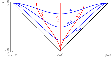
Figure 1: Conformal diagram of 2D dS space, where both the global coordinates (2) and the planar ones (6) are shown. The latter, usually adopted for cosmic inflation, cover only half of dS space, the inflationary patch.

In order to calculate analytically the entanglement entropy associated to a given region, we include a CFT with a central charge $c\gg 1$, so that its many degrees of freedom dominate the entropy (and in 2D its entanglement entropy is well known), without affecting the dS character of spacetime. The entanglement entropy depends on three ingredients: the quantum state of the CFT, the region under consideration and the UV cutoff selecting the modes included in the analysis. About the first, since we are interested in modelling inflation we consider the Bunch-Davies vacuum. The standard procedure to obtain the entanglement entropy in this state is the following. We first introduce conformal complex coordinates

$$z=e^{-i(\sigma-\varphi)}\,,\qquad\bar{z}=e^{-i(\sigma+\varphi)}\,,\qquad ds^{2}=\frac{1}{\Omega(z,\bar{z})^{2}}\,dzd\bar{z}\,,$$ (3)

with $\Omega=H(1+z\bar{z})/2$. The vacuum state in this coordinate system is known to be the Bunch-Davies (or Hartle-Hawking) vacuum ($z,\bar{z}$ are light-cone coordinates). By means of a conformal transformation, we can then use the flat spacetime well-known result [28], by keeping track of the conformal transformation of the UV cutoff, and obtain the entropy of a single interval

$$S=\frac{c}{6}\log\frac{(z_{1}-z_{2})(\bar{z}_{1}-\bar{z}_{2})}{\epsilon_{1}\epsilon_{2}\,\Omega_{1}\Omega_{2}}\,,$$ (4)

where the subscript denotes quantities calculated at the corresponding endpoint of the interval and $\epsilon$ is the cutoff expressed in the relevant system of coordinates. Written in global coordinates this becomes

$$S=\frac{c}{6}\,\log\frac{2\,[\cos(\sigma_{2}-\sigma_{1})-\cos(\varphi_{2}-\varphi_{1})]}{\cos\sigma_{1}\cos\sigma_{2}\,H^{2}\epsilon_{1}\epsilon_{2}}\,.$$ (5)

In the following, it will be clear that for our purposes it is important to retain the global structure of the Bunch-Davies/Hartle-Hawking vacuum rather than, for instance, considering its late time (simpler) Poincaré limit.

II.3 Modelling the entropy bound

The remaining two ingredients are the region of interest and the UV cutoff of the modes considered. In their choice, we are guided by the aim of modelling, as much as possible, the operational setup giving the entropy bound, described in Sec. II.1.

We do not have an inflaton. However, in modelling the setup above we may take it as a clock and reason in terms of the usual planar coordinates of inflation (shown in Fig. 1):

$$ds^{2}=-dt^{2}+e^{2Ht}dx^{2}\,,\qquad e^{Ht}=\frac{\cos\varphi+\sin\sigma}{\cos\sigma}\,,\qquad Hx=\frac{\sin\varphi}{\cos\varphi+\sin\sigma}\,,$$ (6)

with $-\infty<t,x<+\infty$, imagining that dS ends at some fixed time $t_{0}$, modelling the inflaton value for reheating. Then, Minkowski evolution starts and an observer, after some time, will have access to the CFT inflationary modes at the reheating surface, associating an entropy to these. As a consequence, the entropy appearing in the operational setup of Sec. II.1 is nothing but the fine-grained (entanglement) entropy of a region $\mathcal{R}$ given by an interval $(-x,x)$ at fixed $t=t_{0}$. This is sketched in Fig. 2.

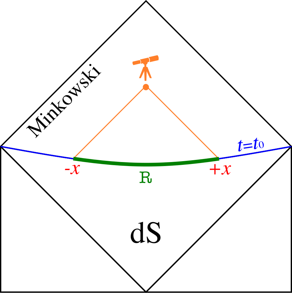
Figure 2: Sketch of the framework modelling the operational setup of Sec. II.1. The dS stage ends at $t=t_{0}$ and Minkowski evolution starts. After some time, a Minkowskian observer (orange dot) is able to observe the inflationary modes in the region $\mathcal{R}$.

The last ingredient is the UV cutoff. While originally the UV cutoff is introduced to regulate the divergence for an interval of vanishing length, we assume that it can be interpreted as the cutoff of the relevant modes, whose entropy one is focused on. In order to model the setup of Sec. II.1, we choose a cutoff

$$\epsilon\sim\frac{1}{H}\,,$$ (7)

i.e at $t=t_{0}$ we consider all and only those modes that have been frozen during inflation. These are precisely the ones that the future Minkowskian observer can reconstruct, for instance from the CMB, in the argument of Sec. II.1. We anticipate that in the next Section we will argue that this prescription is suitable for the region $\mathcal{R}$, but not for the island in the gravitating dS region.

Having specified all the relevant ingredients, we can now calculate the semiclassical entropy seen by the future observer, by combining (5), (6) and (7), and obtain the simple result

$$S_{\rm semi}\simeq\frac{c}{3}\log\frac{2e^{Ht_{0}}x}{\epsilon}\sim\frac{c}{3}\log(Hl_{\mathcal{R}})\;,$$ (8)

having introduced $l_{\mathcal{R}}=2e^{Ht_{0}}x$, the proper length of $\mathcal{R}$. The entropy is simply counting the modes that exited the horizon during inflation.

Finally, let us see how the argument of Sec. II.1 is reproduced. Let us analogously assume that inflation starts at some time $t_{i}<0$. Starting from a single Hubble patch, inflation fills a comoving distance $x\sim e^{-Ht_{i}}/H$. Then, (8) and (7) give that the maximal semiclassical entropy that the Minkowskian observer is able to reconstruct (sufficiently in the future) is:

$$S_{\rm semi}\sim\frac{c}{3}\log\frac{e^{H(t_{0}-t_{i})}}{H\epsilon}\sim\frac{c}{3}\log e^{H(t_{0}-t_{i})}\sim\mathcal{N}_{e}\,,$$ (9)

as in Sec. II.1. When this fine-grained entropy becomes larger than the thermodynamic dS entropy $S_{\rm dS}\sim 2\phi_{0}$ we have an apparent paradox, since the latter measures the total number of states available to the quantum system that should be describing dS space.

III The entropy after a long period of inflation

The enormous progress of the last few years in the understanding of the BH information paradox [3, 4, 5, 6, 7, 8] is based on the appreciation that for a system produced gravitationally a semiclassical entropy such as (8) fails to give the correct result, at late times. Instead, the correct fine-grained entropy is given by the island formula [9, 10, 11, 12, 13, 5]:

$$S(\mathcal{R})=\min\mathrm{ext}_{\mathcal{I}}\left(\frac{\text{Area}(\partial\mathcal{I})}{4}+S_{\rm semi}(\mathcal{R}\cup\mathcal{I})\right)\,,$$ (10)

where the island $\mathcal{I}$ is in the gravitating region and the minimum among the different extrema (including $\mathcal{I}=\varnothing$) is taken. The area of the island boundary $\partial\mathcal{I}$ is in Planck units. Its explicit proof for eternal BHs in 2D gravity [6, 7] suggests the following interpretation. In QFT the entanglement entropy is calculated in terms of Euclidean path integrals on appropriate replica manifolds, where the different sheets are connected by cuts in the region of interest $\mathcal{R}$. In general, since in the gravitational path integral spacetime itself is dynamical, the dominant configurations may contain extra cuts on $\mathcal{I}$, if gravity is allowed to “decide” the replica topology, as dominant saddles in the Euclidean gravitational path-intergral. The extra cuts introduce conical singularities at their boundary, captured by the area term in (10), which gives the entropic contribution of gravity itself.

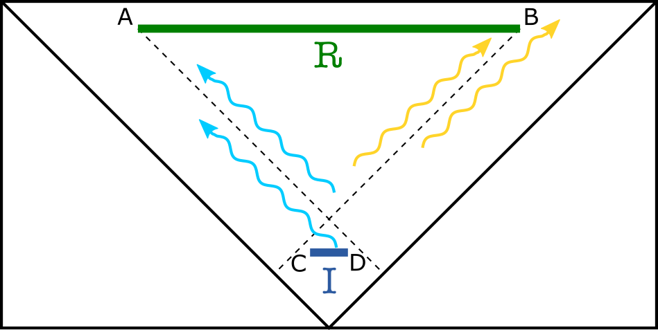
Figure 3: Island contribution to the entropy. The island $\mathcal{I}$ is shown as a cut joining the two endpoints from “inside”. We show modes that stop contributing to the entropy of $\mathcal{R}$ when the island $\mathcal{I}$ is included. Pairs with the same colour are entangled.

Therefore, we look for an island in the setup considered so far. Since we do not know a priori if we will be in a simplifying universal limit (where the CFT entropy is simplified by an OPE), we consider the two-intervals entropy formula. This is known only for a specific CFT, namely $c$ free fermions, so that we now restrict to this case. As before, we can do a conformal transformation from conformal complex coordinates and use the flat-space vacuum entropy [29] to obtain

$$S=\frac{c}{6}\log\frac{\ell^{2}_{AB}\ell^{2}_{BC}\ell^{2}_{CD}\ell^{2}_{DA}}{\ell^{2}_{AC}\ell^{2}_{BD}\epsilon_{A}\epsilon_{B}\epsilon_{C}\epsilon_{D}\Omega_{A}\Omega_{B}\Omega_{C}\Omega_{D}}\,,$$ (11)

where the different letters label the endpoints of $\mathcal{R}$ and $\mathcal{I}$ as denoted in Fig. 3 and we have introduced the short-hand notation $\ell^{2}_{XY}\equiv(z_{X}-z_{Y})(\bar{z}_{X}-\bar{z}_{Y})$.

Notice that the points $C$ and $D$ (as well as $A$ and $B$) are differentiated by the different direction of wrapping around them to move to the same replica sheet. In particular, a counter-clockwise wrapping of $2\pi$ around $A$ and $C$ shifts the replica sheet as $n\to n+1$, whereas as $n\to n-1$ for $B$ and $D$. As a consequence, swapping $C$ and $D$ while keeping $A$ and $B$ fixed changes the replica manifold and hence the entropy.

From (11) and Fig. 3 we may already understand why an island, if appearing, can compete with the semiclassical entropy (8) beating the penalty for the area term in (10). In the limit in which $BC$ and $AD$ become light-like their contribution suppresses the numerator of (11) and compensates for the large contribution of $AB$ (which essentially gives the semiclassical entropy (8)). Moreover, the area term

$$\frac{\text{Area}(\partial\mathcal{I})}{4}=2\phi_{0}+2\phi_{r}\tan\sigma_{\mathcal{I}}$$ (12)

becomes smaller and smaller going towards the past. Here we have set $4G=1$ (which is a normalization for $\phi_{0}$) and taken $\sigma_{C}=\sigma_{D}\equiv\sigma_{\mathcal{I}}$. Below, we will find that the OPE approximation is not appropriate for the determination of the dominant island, since this appears only when the full structure in (11) is retained. Therefore, we cannot know whether our results extrapolate to a generic CFT or not.

While the cutoffs $\epsilon_{A},\epsilon_{B}$ in (11) are in the region $\mathcal{R}$ and can be hence chosen at will, e.g. as given by (7), the situation is different for the the cutoffs $\epsilon_{C},\epsilon_{D}$ in the island region. This is because even if we focus on a subset of all modes (the ones that have been frozen during inflation), the emergent cut in the replica manifold given by the island affects all modes in the theory, even if they are traced over in $\mathcal{R}$. Therefore, the inclusion of this cut for them is equivalent to consider the CFT entropy as cut off by the real UV cutoff of the theory $\epsilon_{\rm UV}$ (presumably a proper length, because of covariance). Then, the standard lore (see e.g. [30, 17]) is that the UV divergence is absorbed into the renormalization of the inverse gravitational coupling $\phi_{0}$, so that the full result (10) is finite. Effectively, one replaces $\epsilon_{\rm UV}\to\epsilon_{\rm RG}$, the renormalization scale that we leave unspecified.

Taking this into account, the two-intervals entropy (11) in global coordinates becomes

$$S_{\rm semi}=\frac{c}{6}\log\frac{4\,(1-\cos 2\varphi_{\mathcal{R}})(1-\cos 2\varphi_{\mathcal{I}})}{H^{4}\epsilon_{\rm RG}^{2}\epsilon^{2}\cos^{2}\sigma_{\mathcal{R}}\cos^{2}\sigma_{\mathcal{I}}}\frac{[\cos(\sigma_{\mathcal{R}}-\sigma_{\mathcal{I}})-\cos(\varphi_{\mathcal{R}}+\varphi_{\mathcal{I}})]^{2}}{[\cos(\sigma_{\mathcal{R}}-\sigma_{\mathcal{I}})-\cos(\varphi_{\mathcal{R}}-\varphi_{\mathcal{I}})]^{2}}\,,$$ (13)

where we have already used symmetry to impose $\sigma_{A}=\sigma_{B}\equiv\sigma_{\mathcal{R}}$, $\varphi_{B}=-\varphi_{A}\equiv\varphi_{\mathcal{R}}>0$, $\varphi_{D}=-\varphi_{C}\equiv\varphi_{\mathcal{I}}$. In view of the discussion above after (11), positive and negative values of $\varphi_{\mathcal{I}}$ correspond to different replica manifolds, where $C$ and $D$ are swapped.

The total entropy in the presence of the island is

$$S(\sigma_{\mathcal{I}},\varphi_{\mathcal{I}})=2\phi_{0}+2\phi_{r}\tan\sigma_{\mathcal{I}}+S_{\rm semi}\,,$$ (14)

with $S_{\rm semi}$ as given in (13). We need to find the extrema of this quantity. This is best done numerically, as shown in Figs. 4 and 5 for $t_{0}\to\infty$. There are several extrema. In the close past (Fig. 5a) there is a minimax (i.e. minimal in time, maximal in space) saddle-point. This is analogous to the island found in [16] in a similar setup, which is argued to be pathological, since it violates the strong-sub-additivity condition by a large amount. The fact that $\varphi_{\mathcal{I}}$ is negative just means that the direction of wrapping around the island endpoints is swapped, as explained above after (13). However, we find that the dominant extremum (the one with minimal $S$, as prescribed by the island formula) is in the distant past, as shown in Fig. 5b. This is a local maximum of $S$. While the former extremum is captured by the OPE approximation and the Poincaré limit of the vacuum, the island $\mathcal{I}$ is present only when the full structure (11) is retained.

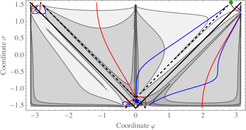
Figure 4: Isocontours of the island entropy $S$ as given in (14) (shaded in lighter gray for larger $S$) and contours of vanishing partial derivatives with respect to $\sigma_{I}$ (blue lines) and $\varphi_{I}$ (red lines). The green dot denotes the endpoint $B$ of the region $\mathcal{R}$, at large times $t_{0}\to\infty$, i.e. $\sigma_{\mathcal{R}}=\pi/2$, while the blue dot denotes the island endpoint $D$. The dashed lines indicate the past lightcone of $\mathcal{R}$.

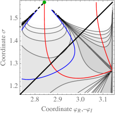
(a)

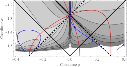
(b)

Figure 5: Zoom of Fig. 4 in the regions in the close and distant past (left and right panels, respectively). Extrema of $S$ arise at the intersection of blue and red lines. In addition to the island, denoted by the blue dot, other extrema are also present, but the corresponding entropy is larger (lighter shading). In the left panel, for convenience we have swapped the sign of the island coordinate $\varphi_{\mathcal{I}}\to-\varphi_{\mathcal{I}}$, see text.

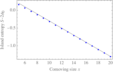
Figure 6: Analytic approximation to the island entropy (continuous line), compared to the full numerical results (blue dots) for $t_{0}\to\infty$. We worked in Hubble units and chose the example values of the parameters $c=1$, $\phi_{r}=0.1$, $\varepsilon=0.1$, $\epsilon_{\rm RG}=1$.

Having established the existence of the island, we can approximate its entropy analytically for $t_{0}\to\infty$ and $\delta\equiv\pi-\varphi_{\mathcal{R}}\simeq 2/Hx\to 0$. This is done by expanding $\partial S/\partial\varphi_{I}=\partial S/\partial\sigma_{I}=0$ for small $\varphi_{\mathcal{I}}$ and $\sigma_{\mathcal{I}}+\pi/2$ and finding the approximate location of the island:

$$\varphi_{\mathcal{I}}\simeq\frac{c}{12\phi_{r}}\delta^{2}\,,\qquad\sigma_{\mathcal{I}}+\frac{\pi}{2}\simeq\delta-\frac{c}{6\phi_{r}}\delta^{2}\,.$$ (15)

Then, we can restore a finite $t_{0}$, i.e. a finite $\pi/2-\sigma_{\mathcal{R}}$, only in the factor $\cos\sigma_{\mathcal{R}}$ in (13), which is formally singular in the $t_{0}\to\infty$ limit. We thus obtain the approximate form of the fine-grained entropy:

$$S(\mathcal{R})\simeq\min\bigg{\{}\frac{c}{3}\log\frac{2e^{Ht_{0}}x}{\epsilon},\;2\phi_{0}-\phi_{r}Hx+\frac{c}{3}\bigg{(}\log\frac{2e^{Ht_{0}}c}{9\phi_{r}H^{2}\epsilon_{\rm RG}\epsilon}-1\bigg{)}\bigg{\}}\,,$$ (16)

having included the no-island contribution. In Fig. 6, we compare the analytical approximation of the island contribution to the full numerical result, showing that the former is indeed sufficiently accurate. The fine-grained entropy can be expressed directly in terms of physical quantities $l_{\mathcal{R}}$, $\phi_{r}^{\rm ph}\equiv\phi_{r}/e^{Ht_{0}}$ as

$$S(\mathcal{R})\simeq\min\bigg{\{}\frac{c}{3}\log(Hl_{\mathcal{R}}),\;2\phi_{0}-\frac{\phi_{r}^{\rm ph}Hl_{\mathcal{R}}}{2}+\frac{c}{3}\bigg{(}\log\frac{2c}{9\phi_{r}^{\rm ph}H\epsilon_{\rm RG}}-1\bigg{)}\bigg{\}}\,.$$ (17)

The entropy of $\mathcal{R}$ follows a Page-like curve, as also shown in Fig. 7. As a consequence, the Minkowskian future observer of Sec. II.1 is never able to measure an entropy larger than the thermodynamic one and the paradox disappears. This suggests that the semiclassical expectation should be modified in such a way that the entropy bound might actually not be present.

IV Discussion and conclusions

To summarize, the basic assumptions that lead to the Page-like curve for the entropy, as reconstructed by the Minkowskian observer, are the following

1. The operational setup that gives the entropy bound can be (toy-)modelled by 2D gravity with a CFT with large central charge.

2. The island formula gives the correct fine-grained entropy in the dS setup considered, in particular for an island not on the same Cauchy slice as the region of interest.

3. In this context a local maximum is a legitimate extremum for the island formula.

Under these assumptions, we have found that the fine-grained entropy is given by (16) and, in particular, never exceeds the thermodynamic dS entropy $S_{\rm dS}\sim 2\phi_{0}$.

In detail, we found that the island contribution dominates for comoving sizes larger than $x_{*}$, with

$$Hx_{*}\simeq\frac{2\phi_{0}}{\phi_{r}}-\frac{c}{3\phi_{r}}\log\frac{2e^{Ht_{0}}x_{*}}{\epsilon}\,,$$ (18)

and the maximal entropy is $S_{*}=S(x_{*})\approx\frac{c}{3}\log(4\phi_{0}/\phi_{r}^{\rm ph})$.

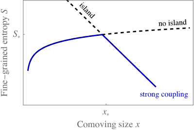
Figure 7: Page-like curve for the fine-grained entropy, as function of the comoving size $2x$ of the region $\mathcal{R}$, at $t_{0}\to\infty$.

Notice that $S_{*}$ is generally much smaller than $S_{\rm dS}$. However, this might be a peculiarity of the 2D toy-model, since it is ultimately due to the fact that both the past light-cone and horizon areas go to zero (in Planck units) in the far past, for the theory (1) (see also Fig. 3). Instead, for 4D dS spacetime, they both tend to $M_{\rm Pl}^{2}/H^{2}$. If our results could be extrapolated to 4D, we would then expect a Page-like curve in which the fine-grained entropy saturates to a constant $S\approx S_{\rm dS}=M_{\rm Pl}^{2}/H^{2}$, rather than decreasing, as in Fig. 7. Nevertheless, a direct 4D calculation looks unfeasible, since the entanglement entropy of a CFT is much less known in this case, and the CFT gravitates.

Let us comment on point 2 above. The island found in this work is not on the same Cauchy slice as the region $\mathcal{R}$ (since it is time-like separated from it) and for this reason an interpretation of the island formula in terms of the entanglement between $\mathcal{R}$ and $\mathcal{I}$ looks involved. At first sight, such interpretation appears to make sense only if $\mathcal{R}$ and $\mathcal{I}$ are independent subsystems, being part of the same Cauchy slice. Therefore, it would be interesting to investigate further the quantum-information meaning of time-like separated islands, such as the one that we found.

Here, we just give some intuitive considerations. As shown in Fig. 3, even though $\mathcal{I}$ and $\mathcal{R}$ are not on the same Cauchy slice, they “almost” are, although in an unusual sense: all light-like trajectories (the ones relevant for the CFT) may intersect either $\mathcal{I}$ and $\mathcal{R}$, but not both. In this sense, for the CFT they are independent systems. The key point is then, as shown in Fig. 3, many entangled pairs naively contributing to the entropy of $\mathcal{R}$ are indeed purified by $\mathcal{I}$, and this is the extremal surface achieving that. This is why the island calculation corrects the naive semiclassical expectation.

We do not know which saddles should be included in the Euclidean gravitational path integral, and what constitutes a legitimate extremum for the island formula, in particular whether a local maximum, such as our result, is acceptable. In the BH context the only legitimate islands are thought to be maximin saddle-points (maximal along time, minimal along space). In the dS case this is not known, especially for a time-like separated island such as ours. We can only check that the obtained entropy is free of obvious pathologies. In a context similar to ours, the authors of [16] found a minimax island (minimal along time, maximal along space), but then argued that it violates the strong-subadditivity condition, a basic criterion for entropies. In Appendix A, we review their argument and show that our island does not lead to a similar paradox. Finally, notice that the entropy (13) is real, as it should be, thanks to the fact that both $BC$ and $BD$ are time-like, a property that in turn implies the quasi-Cauchy property discussed above.

To conclude, if our results could be extrapolated to 4D, they would suggest that the entropy bound on the duration of dS is actually absent. This is not the only obstruction to the possibility of a long (but possibly finite) stage of dS evolution [31, 32, 33, 34, 35], and thus it would certainly be interesting to investigate whether these other arguments could be affected, in a similar way, by the considerations presented here. For instance, the argument of [36] to corroborate the dS conjecture of [33, 34], is precisely based on the entropy bound in the presence of many degrees of freedom. It would be interesting, albeit challenging, to study the consequences of our findings for these matters in future work.

Appendix A No strong-subadditivity paradox

In a similar context to ours, the authors of [16] found an island under certain assumptions, analogous to our subdominant extremum in Fig. 5a and argued that this is pathological, because it violates the strong-subadditivity (SSA) condition

$$S(\mathcal{A}\cup\mathcal{B})+S(\mathcal{A}\cup\mathcal{C})\geq S(\mathcal{A})+S(\mathcal{A}\cup\mathcal{B}\cup\mathcal{C})\,,$$ (19)

which is a basic requirement for an entropy. Their argument goes as follows. One introduces a probe CFT with a small central charge $c_{p}\ll c$, which does not affect the location of the island. In the flat region the two CFTs can be considered as distinct systems. Then, since even in their case $x_{*}$ is a decreasing function of $c$, one can choose a region $\mathcal{R}$ such that the island dominates for $c$ but not for $c_{p}$. Then, the SSA can be calculated for the three distinct systems $\mathcal{R}_{c}$, $\mathcal{R}_{c_{p}}$, $\overline{\mathcal{R}}_{c_{p}}$, obtaining:

$$S(\mathcal{R}_{c}\cup\mathcal{R}_{c_{p}})+S(\overline{\mathcal{R}}_{c_{p}}\cup\mathcal{R}_{c_{p}})-S(\mathcal{R}_{c}\cup\overline{\mathcal{R}}_{c_{p}}\cup\mathcal{R}_{c_{p}})-S(\mathcal{R}_{c_{p}})\simeq-\frac{2c_{p}}{3}\log\frac{l_{\mathcal{R}}c}{\phi_{r}}\ll-1\,$$ (20)

so that the SSA condition is violated by a large universal amount, logarithmic in the size of $\mathcal{R}$.

We can repeat an analogous argument in our case. The two CFTs are not interacting, so

$$S(\overline{\mathcal{R}}_{c_{p}}\cup\mathcal{R}_{c_{p}})=0\,.$$ (21)

For the probe CFT the non-island entropy is dominating, therefore:

$$S(\mathcal{R}_{c_{p}})\simeq\frac{c_{p}}{3}\log\frac{2xe^{Ht_{0}}}{\epsilon}\,.$$ (22)

The fine-grained entropy of an interval for both CFTs is given by

$$S(\mathcal{R}_{c}\cup\mathcal{R}_{c_{p}})\simeq 2\phi_{0}-\phi_{r}Hx+\frac{c+c_{p}}{3}\bigg{(}\log\frac{2e^{Ht_{0}}(c+c_{p})}{9\phi_{r}H^{2}\epsilon_{\rm RG}\epsilon}-1\bigg{)}\,.$$ (23)

Finally, the entropy of the three subsystems is obtained by neglecting the effect of the probe CFT on the location of the island. However, the cut in the replica manifold given by the island affects all fields, including the probe CFT. The total entropy is thus given by the two-interval result for $c$, plus the $c_{p}$ single-interval result on the island:

$$S(\mathcal{R}_{c}\cup\overline{\mathcal{R}}_{c_{p}}\cup\mathcal{R}_{c_{p}})\simeq 2\phi_{0}-\phi_{r}Hx+\frac{c}{3}\bigg{(}\log\frac{2e^{Ht_{0}}c}{9\phi_{r}H^{2}\epsilon_{\rm RG}\epsilon}-1\bigg{)}+\frac{c_{p}}{3}\log\frac{c}{3H^{2}\epsilon_{\rm RG}\phi_{r}x}\,.$$ (24)

All in all, we obtain:

$$S(\mathcal{R}_{c}\cup\mathcal{R}_{c_{p}})+S(\overline{\mathcal{R}}_{c_{p}}\cup\mathcal{R}_{c_{p}})-S(\mathcal{R}_{c}\cup\overline{\mathcal{R}}_{c_{p}}\cup\mathcal{R}_{c_{p}})-S(\mathcal{R}_{c_{p}})\simeq\frac{c_{p}}{3}\log\frac{1}{3}\approx 0\,,$$ (25)

which vanishes within the approximations of our formulas (which in particular disregard the non-logarithmically-enhanced part of the entropy of a CFT). Therefore, our results do not violate the SSA condition (at least in this setup), but rather saturate it.

References

- [1] N. Arkani-Hamed, S. Dubovsky, A. Nicolis, E. Trincherini, and G. Villadoro, “A Measure of de Sitter entropy and eternal inflation,” JHEP 05 (2007) 055, arXiv:0704.1814 [hep-th].
- [2] S. W. Hawking, “Breakdown of Predictability in Gravitational Collapse,” Phys. Rev. D 14 (1976) 2460–2473.
- [3] G. Penington, “Entanglement Wedge Reconstruction and the Information Paradox,” JHEP 09 (2020) 002, arXiv:1905.08255 [hep-th].
- [4] A. Almheiri, N. Engelhardt, D. Marolf, and H. Maxfield, “The entropy of bulk quantum fields and the entanglement wedge of an evaporating black hole,” JHEP 12 (2019) 063, arXiv:1905.08762 [hep-th].
- [5] A. Almheiri, R. Mahajan, J. Maldacena, and Y. Zhao, “The Page curve of Hawking radiation from semiclassical geometry,” JHEP 03 (2020) 149, arXiv:1908.10996 [hep-th].
- [6] G. Penington, S. H. Shenker, D. Stanford, and Z. Yang, “Replica wormholes and the black hole interior,” arXiv:1911.11977 [hep-th].
- [7] A. Almheiri, T. Hartman, J. Maldacena, E. Shaghoulian, and A. Tajdini, “Replica Wormholes and the Entropy of Hawking Radiation,” JHEP 05 (2020) 013, arXiv:1911.12333 [hep-th].
- [8] A. Almheiri, T. Hartman, J. Maldacena, E. Shaghoulian, and A. Tajdini, “The entropy of Hawking radiation,” Rev. Mod. Phys. 93 (2021) no. 3, 035002, arXiv:2006.06872 [hep-th].
- [9] S. Ryu and T. Takayanagi, “Holographic derivation of entanglement entropy from AdS/CFT,” Phys. Rev. Lett. 96 (2006) 181602, arXiv:hep-th/0603001.
- [10] S. Ryu and T. Takayanagi, “Aspects of Holographic Entanglement Entropy,” JHEP 08 (2006) 045, arXiv:hep-th/0605073.
- [11] V. E. Hubeny, M. Rangamani, and T. Takayanagi, “A Covariant holographic entanglement entropy proposal,” JHEP 07 (2007) 062, arXiv:0705.0016 [hep-th].
- [12] T. Faulkner, A. Lewkowycz, and J. Maldacena, “Quantum corrections to holographic entanglement entropy,” JHEP 11 (2013) 074, arXiv:1307.2892 [hep-th].
- [13] N. Engelhardt and A. C. Wall, “Quantum Extremal Surfaces: Holographic Entanglement Entropy beyond the Classical Regime,” JHEP 01 (2015) 073, arXiv:1408.3203 [hep-th].
- [14] D. N. Page, “Information in black hole radiation,” Phys. Rev. Lett. 71 (1993) 3743–3746, arXiv:hep-th/9306083.
- [15] D. N. Page, “Time Dependence of Hawking Radiation Entropy,” JCAP 09 (2013) 028, arXiv:1301.4995 [hep-th].
- [16] Y. Chen, V. Gorbenko, and J. Maldacena, “Bra-ket wormholes in gravitationally prepared states,” JHEP 02 (2021) 009, arXiv:2007.16091 [hep-th].
- [17] T. Hartman, Y. Jiang, and E. Shaghoulian, “Islands in cosmology,” JHEP 11 (2020) 111, arXiv:2008.01022 [hep-th].
- [18] L. Aalsma and W. Sybesma, “The Price of Curiosity: Information Recovery in de Sitter Space,” JHEP 05 (2021) 291, arXiv:2104.00006 [hep-th].
- [19] K. Langhoff, C. Murdia, and Y. Nomura, “Multiverse in an inverted island,” Phys. Rev. D 104 (2021) no. 8, 086007, arXiv:2106.05271 [hep-th].
- [20] S. E. Aguilar-Gutierrez, A. Chatwin-Davies, T. Hertog, N. Pinzani-Fokeeva, and B. Robinson, “Islands in Multiverse Models,” arXiv:2108.01278 [hep-th].
- [21] J. Kames-King, E. Verheijden, and E. Verlinde, “No Page Curves for the de Sitter Horizon,” arXiv:2108.09318 [hep-th].
- [22] E. Shaghoulian, “The central dogma and cosmological horizons,” arXiv:2110.13210 [hep-th].
- [23] R. Jackiw, “Lower Dimensional Gravity,” Nucl. Phys. B 252 (1985) 343–356.
- [24] C. Teitelboim, “Gravitation and Hamiltonian Structure in Two Space-Time Dimensions,” Phys. Lett. B 126 (1983) 41–45.
- [25] A. Almheiri and J. Polchinski, “Models of AdS2 backreaction and holography,” JHEP 11 (2015) 014, arXiv:1402.6334 [hep-th].
- [26] J. Maldacena, G. J. Turiaci, and Z. Yang, “Two dimensional Nearly de Sitter gravity,” JHEP 01 (2021) 139, arXiv:1904.01911 [hep-th].
- [27] J. Cotler, K. Jensen, and A. Maloney, “Low-dimensional de Sitter quantum gravity,” JHEP 06 (2020) 048, arXiv:1905.03780 [hep-th].
- [28] P. Calabrese and J. L. Cardy, “Entanglement entropy and quantum field theory,” J. Stat. Mech. 0406 (2004) P06002, arXiv:hep-th/0405152.
- [29] H. Casini, C. D. Fosco, and M. Huerta, “Entanglement and alpha entropies for a massive Dirac field in two dimensions,” J. Stat. Mech. 0507 (2005) P07007, arXiv:cond-mat/0505563.
- [30] R. Bousso, Z. Fisher, S. Leichenauer, and A. C. Wall, “Quantum focusing conjecture,” Phys. Rev. D 93 (2016) no. 6, 064044, arXiv:1506.02669 [hep-th].
- [31] S. Dubovsky, L. Senatore, and G. Villadoro, “The Volume of the Universe after Inflation and de Sitter Entropy,” JHEP 04 (2009) 118, arXiv:0812.2246 [hep-th].
- [32] G. Dvali and C. Gomez, “Quantum Exclusion of Positive Cosmological Constant?,” Annalen Phys. 528 (2016) 68–73, arXiv:1412.8077 [hep-th].
- [33] G. Obied, H. Ooguri, L. Spodyneiko, and C. Vafa, “De Sitter Space and the Swampland,” arXiv:1806.08362 [hep-th].
- [34] S. K. Garg and C. Krishnan, “Bounds on Slow Roll and the de Sitter Swampland,” JHEP 11 (2019) 075, arXiv:1807.05193 [hep-th].
- [35] G. Dvali, “On -Matrix Exclusion of de Sitter and Naturalness,” arXiv:2105.08411 [hep-th].
- [36] H. Ooguri, E. Palti, G. Shiu, and C. Vafa, “Distance and de Sitter Conjectures on the Swampland,” Phys. Lett. B 788 (2019) 180–184, arXiv:1810.05506 [hep-th].