Ref-NeRF: Structured View-Dependent Appearance for Neural Radiance Fields

Abstract

Neural Radiance Fields (NeRF) is a popular view synthesis technique that represents a scene as a continuous volumetric function, parameterized by multilayer perceptrons that provide the volume density and view-dependent emitted radiance at each location. While NeRF-based techniques excel at representing fine geometric structures with smoothly varying view-dependent appearance, they often fail to accurately capture and reproduce the appearance of glossy surfaces. We address this limitation by introducing Ref-NeRF, which replaces NeRF’s parameterization of view-dependent outgoing radiance with a representation of reflected radiance and structures this function using a collection of spatially-varying scene properties. We show that together with a regularizer on normal vectors, our model significantly improves the realism and accuracy of specular reflections. Furthermore, we show that our model’s internal representation of outgoing radiance is interpretable and useful for scene editing.

Ground Truth

Ours

Mip-NeRF [2]

PSNR$\uparrow$/MAE$\downarrow$:

$\mathbf{35.6}$dB/$\mathbf{11.5^{\circ}}$

$30.3$dB/$59.5^{\circ}$

Figure 1: Ref-NeRF significantly improves normal vectors (top row) and visual realism (remaining rows) compared to mip-NeRF, the previous top-performing neural view synthesis model. Ref-NeRF’s improvements are apparent in rendered frames (Rows 2 & 3), and even more in rendered videos (bottom row epipolar plane images and supplementary video), where its glossy highlights shift realistically across views instead of blurring and fading like mip-NeRF’s. Image PSNR (higher is better) and surface normal mean angular error (lower is better) shown as insets.

1 Introduction

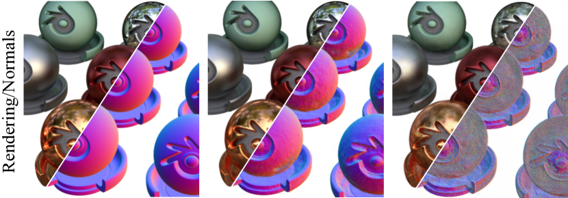
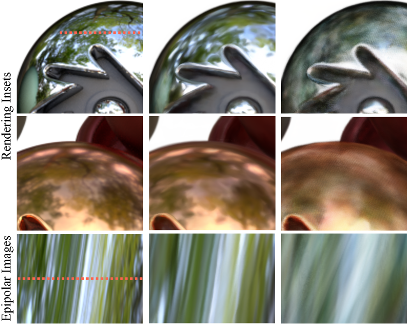
Neural Radiance Fields (NeRF) [24] renders compelling photorealistic images of 3D scenes from novel viewpoints using a neural volumetric scene representation. Given any input 3D coordinate in the scene, a “spatial” multilayer perceptron (MLP) outputs the corresponding volume density at that point, and a “directional” MLP outputs the outgoing radiance at that point along any input viewing direction. Although NeRF’s renderings of view-dependent appearance may appear reasonable at first glance, a close inspection of specular highlights reveals spurious glossy artifacts that fade in and out between rendered views (Figure 1), rather than smoothly moving across surfaces in a physically-plausible manner.

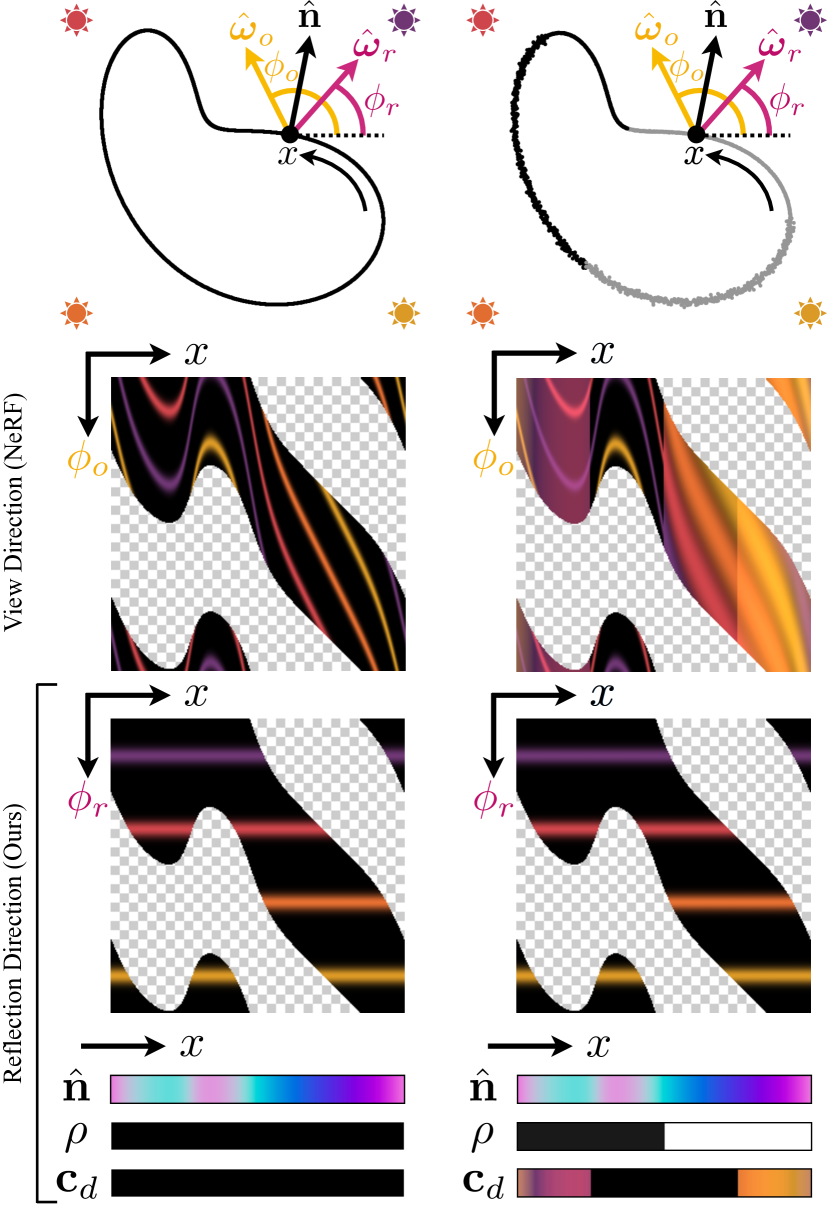
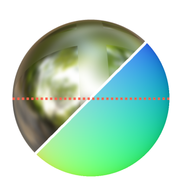
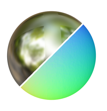
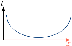
These artifacts are caused by two fundamental issues with NeRF (and top-performing extensions such as mip-NeRF [2]). First, NeRF’s parameterization of the outgoing radiance at each point as a function of the viewing direction is poorly-suited for interpolation. Figure 2 illustrates that, even for a simple toy setup, the scene’s true radiance function varies quickly with view direction, especially around specular highlights. As a consequence, NeRF is only able to accurately render the appearance of scene points from the specific viewing directions observed in the training images, and its interpolation of glossy appearance from novel viewpoints is poor. Second, NeRF tends to “fake” specular reflections using isotropic emitters inside the object instead of view-dependent radiance emitted by points at the surface, resulting in objects with semitransparent or “foggy” shells.

Our key insight is that structuring NeRF’s representation of view-dependent appearance can make the underlying function simpler and easier to interpolate. We present a model, which we call Ref-NeRF, that reparameterizes NeRF’s directional MLP by providing the reflection of the viewing vector about the local normal vector as input instead of the viewing vector itself. Figure 2 (left column) illustrates that, for a toy scene comprised of a glossy object under distant illumination, this reflected radiance function is constant across the scene (ignoring lighting occlusions and interreflections) because it is unaffected by changes in surface orientation. Consequently, since the directional MLP acts as an interpolation kernel, our model is better able to “share” observations of appearance between nearby points to render more realistic view-dependent effects in interpolated views. We additionally introduce an Integrated Directional Encoding technique, and we structure outgoing radiance into explicit diffuse and specular components to allow the reflected radiance function to remain smooth despite variation in material and texture over the scene.

While these improvements crucially enable Ref-NeRF to accurately interpolate view-dependent appearance, they rely on the ability to reflect viewing vectors about normal vectors estimated from NeRF’s volumetric geometry. This presents a problem, as NeRF’s geometry is foggy and not tightly concentrated at surfaces, and its normal vectors are too noisy to be useful for computing reflection directions (as shown in the right column of Figure 1). We ameliorate this issue with a novel regularizer for volume density that significantly improves the quality of NeRF’s normal vectors and encourages volume density to concentrate around surfaces, enabling our model to compute accurate reflection vectors and render realistic specular reflections, shown in Figure 1.

Figure 2: Visualizations of outgoing radiance in NeRF and Ref-NeRF, using 2D position-angle slices of radiance along an $x$-parameterized surface curve on a glossy object under colored lights. Because NeRF (middle row) uses view angle $\phi_{o}$ as input, when presented with glossy reflectances (left) or spatially-varying materials (right) it must interpolate between highly complicated functions like the irregularly curved colored lines shown here. In contrast, Ref-NeRF (bottom row) parameterizes radiance using a normal vector $\hat{\mathbf{n}}$ and a reflection angle $\phi_{r}$, and adds diffuse color $\mathbf{c}_{d}$ and roughness $\rho$ to its spatial MLP, which collectively makes radiance functions simple to model even for shiny or spatially-varying materials. The gray checkerboard indicates directions below the surface at position $x$.

To summarize, we make the following contributions:

1. A reparameterization of NeRF’s outgoing radiance, based on the reflection of the viewing vector about the local normal vector (Section 3.1).

2. An Integrated Directional Encoding (Section 3.2) that, when coupled with a separation of diffuse and specular colors (Section 3.3), enables the reflected radiance function to be smoothly interpolated across scenes with varying materials and textures.

3. A regularization that concentrates volume density around surfaces and improves the orientation of NeRF’s normal vectors (Section 4).

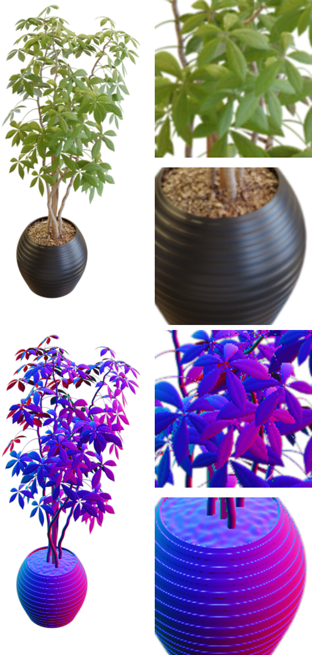
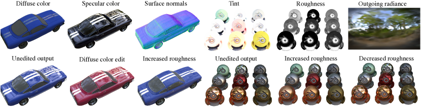
We apply these changes on top of mip-NeRF [2], currently the top-performing neural representation for view synthesis. Our experiments demonstrate that Ref-NeRF produces state-of-the-art renderings of novel viewpoints, and substantially improves upon the quality of previous top-performing view synthesis methods for highly specular or glossy objects. Furthermore, our structuring of outgoing radiance produces interpretable components (normal vectors, material roughness, diffuse texture, and specular tint) that enable convincing scene editing capabilities.

2 Related Work

We review NeRF and related methods for photorealistic view synthesis, as well as techniques from computer graphics for capturing and rendering specular appearance.

3D scene representations for view synthesis

View synthesis, the task of using observed images of a scene to render images from novel unobserved camera viewpoints, is a longstanding research problem within the fields of computer vision and graphics. In situations where it is possible to densely capture images of the scene, simple light field interpolation techniques [12, 18] can render novel views with high fidelity. However, exhaustive sampling of the light field is impractical in most scenarios, so methods for view synthesis from sparsely-captured images reconstruct 3D scene geometry in order to reproject observed images into novel viewpoints [8]. For scenes with glossy surfaces, some methods explicitly build virtual geometry to explain the motion of reflections [35, 17, 33]. Early approaches used triangle meshes as the geometry representation, and rendered novel views by reprojecting and blending multiple captured images with either heuristic [7, 9, 42] or learned [13, 32] blending algorithms. Recent works have used volumetric representations such as voxel grids [20] or multiplane images [10, 23, 37, 41, 48], which are better suited for gradient-based optimization than meshes. While these discrete volumetric representations can be effective for view synthesis, their cubic scaling limits their ability to represent large or high resolution scenes.

The recent paradigm of coordinate-based neural representations replaces traditional discrete representations with an MLP that maps from any continuous input 3D coordinate to the geometry and appearance of the scene at that location. NeRF [24] is an effective coordinate-based neural representation for photorealistic view synthesis that represents a scene as a field of particles that block and emit view-dependent light. NeRF has inspired many subsequent works, which extend its neural volumetric scene representation to application domains including dynamic and deformable scenes [26], avatar animation [11, 27], and even phototourism [21]. Our work focuses on improving a core component of NeRF: the representation of view-dependent appearance. We believe that the improvements presented here can be used to improve rendering quality in many of the applications of NeRF described above.

A key component of our approach considers the reflection of camera rays off NeRF’s geometry. This idea is shared by recent works that extend NeRF to enable relighting by decomposing appearance into scene lighting and materials [3, 4, 5, 36, 45, 47]. Crucially, our model structures the scene into components that are not required to have precise physical meanings, and is thus able to avoid the strong simplifying assumptions (such as known lighting [3, 36], no self-occlusions [4, 5, 45], single-material scenes [45]) that these works need to make to recover explicit parametric representations of lighting and material. Our work also focuses on improving the smoothness and quality of normal vectors extracted from NeRF’s geometry. This goal is shared by recent works that combine NeRF’s neural volumetric representation with neural implicit surface representations [25, 39, 43]. However, these methods primarily focus on the quality of isosurfaces extracted from their representation as opposed to the quality of rendered novel views, and as such their view synthesis performance is significantly worse than top-performing NeRF-like models.

Efficient rendering of glossy appearance

Our work takes inspiration from seminal approaches in computer graphics for representing and rendering view-dependent specular and reflective appearance, particularly techniques based on precomputation [29]. The reflected radiance function encoded in our directional MLP is similar to prefiltered environment maps [15, 31], which were introduced for real-time rendering of specular appearance. Prefiltered environment maps leverage the insight that the outgoing light from a surface can be seen as a spherical convolution of the incoming light and the (radially-symmetric) bidirectional reflectance distribution function (BRDF) that describes the material properties of the surface [30]. After storing this convolution result, rays intersecting the object can be rendered efficiently by simply indexing into the prefiltered environment maps with the reflection direction of the viewing vector about the normal vector.

Instead of rendering predefined 3D assets, our work leverages these computer graphics insights to solve a computer vision problem where we are recovering a renderable model of the scene from images. Furthermore, our directional MLP’s representation of reflected radiance improves upon the prefiltered environment map representations used in computer graphics in a critical way: our directional MLP can represent spatial variation in reflected radiance due to spatial variation in both lighting and scene properties such as material roughness and texture, while the techniques described previously require computing and storing discrete prefiltered radiance maps for each possible material.

Our work is also inspired by a long line of works in computer graphics that reparameterize directional functions such as BRDFs [31, 34] and outgoing radiance [42] for improved interpolation and compression.

Figure 3: We enable the directional MLP to represent reflected radiance functions for any continuously-valued roughness using our integrated directional encoding. Each component of the encoding is a spherical harmonic function convolved with a vMF distribution with concentration parameter $\kappa$, output by our spatial MLP (equivalent to the expectation of the spherical harmonic under the vMF). Less rough locations receive higher-frequency encodings (top), while more rough regions receive encodings with attenuated high frequencies. Our IDE allows lighting information to be shared between locations with different roughnesses, and lets reflectance be edited.

2.1 NeRF Preliminaries

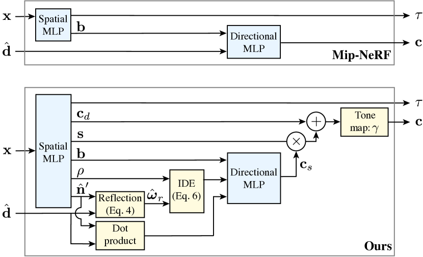
NeRF [24] represents a scene as a volumetric field of particles that emit and absorb light. Given any input 3D position $\mathbf{x}$, NeRF uses a spatial MLP to output the density $\tau(\mathbf{x})$ of volumetric particles as well as a “bottleneck” vector $\mathbf{b}(\mathbf{x})$ which, along with the view direction $\hat{\mathbf{d}}$, is provided to a second directional MLP that outputs the color $\mathbf{c}(\mathbf{x},\hat{\mathbf{d}})$ of light emitted by a particle at that 3D position at direction $\hat{\mathbf{d}}$ (see Figure 4 for a visualization). Note that Mildenhall et al. [24] use a single-layer directional MLP in their work, and that prior work often describes the combination of NeRF’s spatial and directional MLPs as a single MLP.

The two MLPs are queried at points $\mathbf{x}_{i}=\mathbf{o}+t_{i}\hat{\mathbf{d}}$ along a ray originating at $\mathbf{o}$ with direction $\hat{\mathbf{d}}$, and return densities $\{\tau_{i}\}$ and colors $\{\mathbf{c}_{i}\}$. These densities and colors are alpha composited using numerical quadrature [22] to obtain the color of the pixel corresponding to the ray:

$$\mathbf{C}(\mathbf{o},\hat{\mathbf{d}}) =\sum_{i}w_{i}\mathbf{c}_{i}\,,$$ (1)

$$\text{where}\quad w_{i} =e^{-\sum_{j<i}\tau_{j}(t_{j+1}-t_{j})}\left(1-e^{-\tau_{i}(t_{i+1}-t_{i})}\right)\,.$$

The MLP parameters are optimized to minimize the L2 difference between each pixel’s predicted color $\mathbf{C}(\mathbf{o},\hat{\mathbf{d}})$ and its true color $\mathbf{C}_{\mathrm{gt}}(\mathbf{o},\hat{\mathbf{d}})$ taken from the input image:

$$\mathcal{L}=\sum_{\mathbf{o},\hat{\mathbf{d}}}\|\mathbf{C}(\mathbf{o},\hat{\mathbf{d}})-\mathbf{C}_{\mathrm{gt}}(\mathbf{o},\hat{\mathbf{d}})\|^{2}\,.$$ (2)

In practice, NeRF uses two sets of MLPs, one coarse and one fine, in a hierarchical sampling fashion, where both are trained to minimize the loss in Equation 2.

Prior NeRF-based models define a normal vector field in the scene by either using the spatial MLP to predict unit vectors [3, 47] at any 3D location, or by using the gradient of the volume density with respect to 3D position [4, 36]:

$$\hat{\mathbf{n}}(\mathbf{x})=-\frac{\nabla\tau(\mathbf{x})}{\|\nabla\tau(\mathbf{x})\|}\,.$$ (3)

3 Structured View-Dependent Appearance

In this section, we describe how Ref-NeRF structures the outgoing radiance at each point into (prefiltered) incoming radiance, diffuse color, material roughness, and specular tint, which are better-suited for smooth interpolation across the scene than the function of outgoing radiance parameterized by view direction. By explicitly using these components in our directional MLP (Figure 4), Ref-NeRF can accurately reproduce the appearance of specular highlights and reflections. In addition, our model’s decomposition of outgoing radiance enables scene editing.

3.1 Reflection Direction Parameterization

While NeRF directly uses view direction, we instead reparameterize outgoing radiance as a function of the reflection of the view direction about the local normal vector:

$$\hat{\bm{\omega}}_{r}=2(\hat{\bm{\omega}}_{o}\cdot\hat{\mathbf{n}})\hat{\mathbf{n}}-\hat{\bm{\omega}}_{o},$$ (4)

where $\hat{\bm{\omega}}_{o}=-\hat{\mathbf{d}}$ is a unit vector pointing from a point in space to the camera, and $\hat{\mathbf{n}}$ is the normal vector at that point. As demonstrated in Figure 2, this reparameterization makes specular appearance better-suited for interpolation.

For BRDFs that are rotationally-symmetric about the reflected view direction, i.e. ones that satisfy $f(\hat{\bm{\omega}}_{i},\hat{\bm{\omega}}_{o})=p(\hat{\bm{\omega}}_{r}\cdot\hat{\bm{\omega}}_{i})$ for some lobe function $p$ (which includes BRDFs such as Phong [28]), and neglecting phenomena such as interreflections and self-occlusions, view-dependent radiance is a function of the reflection direction $\hat{\bm{\omega}}_{r}$ only:

$$L_{\mathrm{out}}(\hat{\bm{\omega}}_{o})\propto\int L_{\mathrm{in}}(\hat{\bm{\omega}}_{i})p(\hat{\bm{\omega}}_{r}\cdot\hat{\bm{\omega}}_{i})d\hat{\bm{\omega}}_{i}=F(\hat{\bm{\omega}}_{r}).$$ (5)

Thus, by querying the directional MLP with the reflection direction, we are effectively training it to output this integral as a function of $\hat{\bm{\omega}}_{r}$. Because more general BRDFs may vary with the angle between the view direction and normal vector due to phenomena such as Fresnel effects [15], we also input $\hat{\mathbf{n}}\cdot\hat{\bm{\omega}}_{o}$ to the directional MLP to allow the model to adjust the shape of the underlying BRDF.

3.2 Integrated Directional Encoding

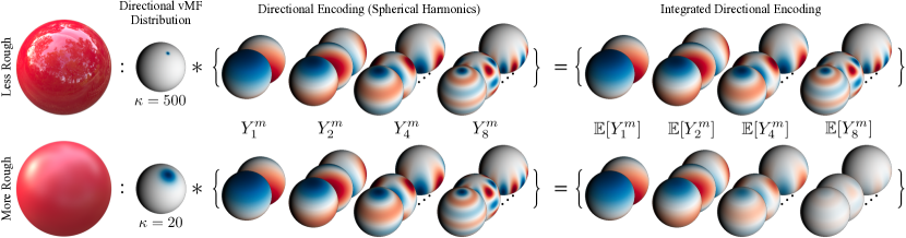
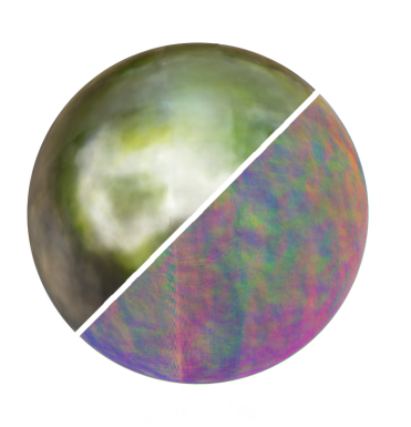
In realistic scenes with spatially-varying materials, radiance cannot be represented as a function of reflection direction alone. The appearance of rougher materials changes slowly with reflection direction, while the appearance of smoother or shinier materials changes rapidly. We introduce a technique, which we call an Integrated Directional Encoding (IDE), that enables the directional MLP to efficiently represent the function of outgoing radiance for materials with any continuously-valued roughness. Our IDE is inspired by the integrated positional encoding introduced by mip-NeRF [2] which enables the spatial MLP to represent prefiltered volume density for anti-aliasing.

First, instead of encoding directions with a set of sinusoids, as done in NeRF, we encode directions with a set of spherical harmonics $\{Y_{\ell}^{m}\}$. This encoding benefits from being stationary on the sphere, a property which is crucial to the effectiveness of positional encoding in Euclidean space [24, 38] (more details in our supplement).

Next, we enable the directional MLP to reason about materials with different roughnesses by encoding a distribution of reflection vectors instead of a single vector. We model this distribution defined on the unit sphere with a von Mises-Fisher (vMF) distribution (also known as a normalized spherical Gaussian), centered at reflection vector $\hat{\bm{\omega}}_{r}$, and with a concentration parameter $\kappa$ defined as inverse roughness $\kappa=\nicefrac{{1}}{{\rho}}$. The roughness $\rho$ is output by the spatial MLP (using a softplus activation) and determines the roughness of the surface: a larger $\rho$ value corresponds to a rougher surface with a wider vMF distribution. Our IDE encodes the distribution of reflection directions using the expected value of a set of spherical harmonics under this vMF distribution:

$$\operatorname{IDE}(\hat{\bm{\omega}}_{r},\kappa) =\left\{\mathbb{E}_{\hat{\bm{\omega}}\sim\operatorname{vMF}(\hat{\bm{\omega}}_{r},\kappa)}[Y_{\ell}^{m}(\hat{\bm{\omega}})]\colon(\ell,m)\in\mathcal{M}_{L}\right\},$$

$$\text{with}\quad\mathcal{M}_{L} =\{(\ell,m)\colon\ell=1,...,2^{L},m=0,...,\ell\}.$$ (6)

In our supplement, we show that the expected value of any spherical harmonic under a vMF distribution has the following simple closed-form expression:

$$\mathbb{E}_{\hat{\bm{\omega}}\sim\operatorname{vMF}(\hat{\bm{\omega}}_{r},\kappa)}[Y_{\ell}^{m}(\hat{\bm{\omega}})]=A_{\ell}(\kappa)Y_{\ell}^{m}(\hat{\bm{\omega}}_{r}),$$ (7)

and that the $\ell$th attenuation function $A_{\ell}(\kappa)$ can be well-approximated using a simple exponential function:

$$A_{\ell}(\kappa)\approx\exp\left(-\frac{\ell(\ell+1)}{2\kappa}\right).$$ (8)

Figure 3 illustrates that our integrated directional encoding has an intuitive behavior; increasing the roughness of a material by lowering $\kappa$ corresponds to attenuating the encoding’s spherical harmonics with high orders $\ell$, resulting in a wider interpolation kernel that limits the high frequencies in the represented view-dependent color.

Figure 4: A visualization of mip-NeRF’s and our architectures.

3.3 Diffuse and Specular Colors

We further simplify the function of outgoing radiance by separating the diffuse and specular components, using the fact that diffuse color is (by definition) a function of only position. We modify the spatial MLP to output a diffuse color $\mathbf{c}_{d}$ and a specular tint $\mathbf{s}$, and we combine this with the specular color $\mathbf{c}_{s}$ provided by the directional MLP to obtain a single color value:

$$\mathbf{c}=\gamma(\mathbf{c}_{d}+\mathbf{s}\odot\mathbf{c}_{s}),$$ (9)

where $\odot$ denotes elementwise multiplication, and $\gamma$ is a fixed tone mapping function that converts linear color to sRGB [1] and clips the output color to lie in $[0,1]$.

3.4 Additional Degrees of Freedom

Effects such as interreflections and self-occlusion of lighting cause illumination to vary spatially over a scene. We therefore additionally pass a bottleneck vector $\mathbf{b}$, output by the spatial MLP, into the directional MLP so the reflected radiance can change with 3D position.

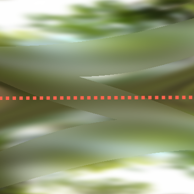
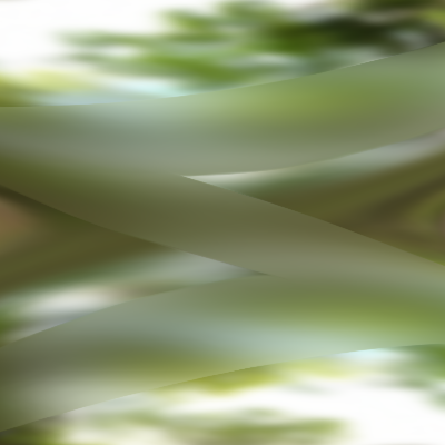
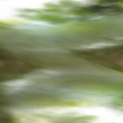
	Ground truth	Ours	Mip-NeRF [2]
Rendering/Normals
	PSNR$\uparrow$/MAE$\downarrow$:	$\mathbf{47.7}$dB/$\mathbf{1.6^{\circ}}$	$23.2$dB/$96.6^{\circ}$
Epipolar Plane Image
Weights $w_{i}$

   

Figure 5: Prior top-performing NeRF-based approaches can fail catastrophically in highly-reflective scenes. Mip-NeRF (right column) produces blurry renderings of reflections that are inconsistent over different views (see EPI), and does not correctly simulate the appearance of the two different surface roughnesses. Our model (middle column) reconstructs the object almost perfectly. The accumulated normals and rendering weights $w_{i}$ along the central scanline of the image (bottom row) show that mip-NeRF mimics specularities using emitters inside the object, while Ref-NeRF correctly recovers a concentrated surface.

4 Accurate Normal Vectors

While the structuring of outgoing radiance described in the previous section provides a better parameterization for the interpolation of specularities, it relies on a good estimation of volume density for facilitating accurate reflection direction vectors. However, the volume density field recovered by NeRF-based models suffers from two limitations: 1) normal vectors estimated from its volume density gradient as in Equation 3 are often extremely noisy (Figures 1 and 5); and 2) NeRF tends to “fake” specular highlights by embedding emitters inside the object and partially occluding them with a “foggy” diffuse surface (see Figure 5). This is a suboptimal explanation, as it requires diffuse content on the surface to be semitransparent so that the embedded emitter can “shine through”.

We address the first issue by using predicted normals for computing reflection directions: for each position $\mathbf{x}_{i}$ along a ray we output a $3$-vector from the spatial MLP, which we then normalize to get a predicted normal $\hat{\mathbf{n}}_{i}^{\prime}$. We tie these predicted normals to the underlying density gradient normal samples along each ray $\{\hat{\mathbf{n}}_{i}\}$ using a simple penalty:

$$\mathcal{R}_{\mathrm{p}}=\sum_{i}w_{i}\|\hat{\mathbf{n}}_{i}-\hat{\mathbf{n}}^{\prime}_{i}\|^{2},$$ (10)

where $w_{i}$ is the weight of the $i$th sample along the ray, as defined in Equation 1. These MLP-predicted normals tend to be smoother than gradient density normals because the gradient operator acts as a high-pass filter on the MLP’s effective interpolation kernel [38].

We address the second issue by introducing a novel regularization term that penalizes normals that are “back-facing”, i.e. oriented away from the camera, at samples along the ray that contribute to the ray’s rendered color:

$$\mathcal{R}_{\mathrm{o}}=\sum_{i}w_{i}\max(0,\hat{\mathbf{n}}^{\prime}_{i}\cdot\hat{\mathbf{d}})^{2}.$$ (11)

This regularization acts as a penalty on “foggy” surfaces: samples are penalized when they are “visible” (high $w_{i}$) and the volume density is decreasing along the ray (i.e. the dot product between $\hat{\mathbf{n}}_{i}^{\prime}$ and ray direction $\hat{\mathbf{d}}$ is positive). This normal orientation penalty prevents our method from explaining specularities as emitters hidden beneath a semitransparent surface, and the resulting improved normals enable Ref-NeRF to compute accurate reflection directions for use in querying the directional MLP.

Throughout the paper, we use the gradient density normals for visualization and quantitative evaluation, as they directly demonstrate the quality of the underlying recovered scene geometry.

5 Experiments

We implement our model on top of mip-NeRF [2], an improved version of NeRF that reduces aliasing. We use the same spatial MLP architecture as mip-NeRF (8 layers, 256 hidden units, ReLU activations), but we use a larger directional MLP (8 layers, 256 hidden units, ReLU activations) than mip-NeRF to better represent high-frequency reflected radiance distributions. Please refer to our supplement for additional baseline implementation details.

We use the same quantitative metrics as previous view synthesis works [24, 2, 45]: PSNR, SSIM [40], and LPIPS [46] are used for evaluating rendering quality, and mean angular error (MAE) is used for evaluating estimated normal vectors.

Shiny Blender Dataset

Though the “Blender” dataset used by NeRF [24] contains a variety of objects with complex geometry, it is severely limited in terms of material variety: most scenes are largely Lambertian. To probe more challenging material properties, we have created an additional “Shiny Blender” dataset with $6$ different glossy objects rendered in Blender under conditions similar to NeRF’s dataset (100 training and 200 testing images per scene). The quantitative results in Table 1 highlight the significant advantage of our model over mip-NeRF, the previous top-performing technique, for rendering novel views of these highly specular scenes. We also include three improved versions of mip-NeRF, all of which have an 8-layer directional MLP and, respectively: 1) no additional components; 2) normal vectors appended to the view direction in the directional MLP (as was done in IDR [44] and VolSDF [43]); and 3) our orientation loss applied to mip-NeRF’s density gradient normal vectors. Our method significantly outperforms all of these improved variants of this previously top-performing neural view synthesis method, both in terms of novel view rendering quality and normal vector accuracy. Although PhySG [45] recovers more accurate normals, it requires ground-truth object masks (all other methods only require RGB images) and produces significantly worse renderings. Figure 5 showcases the impact of our approach using one object from our dataset: while mip-NeRF [2] fails to recover the geometry and appearance of this simple metallic sphere with two roughnesses, our method produces a nearly perfect reconstruction. Figure 9 displays another visual example from this dataset that showcases our model’s improvements to recovered normal vectors and rendered specularities.

	​PSNR $\uparrow$​	​SSIM $\uparrow$​	​LPIPS $\downarrow$​	​$\text{MAE}^{\circ}$ $\downarrow$​
PhySG [45] (requires object masks)	26.21	0.921	0.121	8.46
Mip-NeRF [2]	29.76	0.942	0.092	60.38
Mip-NeRF, 8 layers	31.59	0.956	0.072	58.07
Mip-NeRF, 8 layers, w/ normals	31.39	0.955	0.074	58.27
Mip-NeRF, 8 layers, w/ $\mathcal{R}_{o}$	31.48	0.955	0.073	57.37
Ours, no reflection	29.47	0.944	0.084	16.19
Ours, no $\mathcal{R}_{o}$	31.62	0.954	0.078	52.56
Ours, no pred. normals	30.91	0.936	0.105	30.67
Ours, concat. viewdir	35.42	0.966	0.061	21.25
Ours, fixed lobe	35.52	0.965	0.061	26.46
Ours, no diffuse color	33.32	0.962	0.067	26.13
Ours, no tint	35.45	0.965	0.060	22.70
Ours, no roughness	33.39	0.963	0.065	25.96
Ours, PE	35.90	0.968	0.058	20.31
Ours	35.96	0.967	0.058	18.38

Table 1: Baseline comparisons and ablation study on our “Shiny Blender” dataset.

Table 1 also contains a quantitative ablation study of our model. If we use view directions instead of reflection directions as the directional MLP’s input (“no reflection”), our method’s reconstruction metrics drop significantly, showing the benefits of our reflected radiance parameterization. Removing the orientation loss (“no $\mathcal{R}_{o}$”) results in severely degraded normals and renderings, and applying the orientation loss directly to the density field’s normals and using those to compute reflection directions (“no pred. normals”) also reduces performance. Including the view direction as input to the directional MLP in addition to the IDE (“concat. viewdir”) slightly decreases performance, demonstrating the difficulty of parameterizing specular appearance as a function of viewing direction. On the other hand, not feeding $\hat{\mathbf{n}}^{\prime}\cdot\hat{\bm{\omega}}_{o}$ to the directional MLP (“fixed lobe”) also slightly reduces performance. Finally, removing our structural components of outgoing radiance (roughness, diffuse color, or tint) and replacing our IDE with a non-integrated directional encoding or NeRF’s standard positional encoding all slightly decrease performance.

	​PSNR $\uparrow$​	​SSIM $\uparrow$​	​LPIPS $\downarrow$​	​$\text{MAE}^{\circ}$ $\downarrow$​
PhySG [45] (requires object masks)	20.60	0.861	0.144	29.17
VolSDF [43]	27.96	0.932	0.096	19.45
NSVF [19]	31.74	0.953	0.047	–
NeRF [24]	32.38	0.957	0.046	–
Mip-NeRF [2]	33.09	0.961	0.043	38.30
Ours, PE	33.90	0.965	0.039	24.16
Ours	33.99	0.966	0.038	23.22

Table 2: Results for our method compared to previous approaches on the Blender dataset [24].

	Ground truth	Ours	Mip-NeRF [2]	VolSDF [43]
	PSNR$\uparrow$/MAE$\downarrow$	$\mathbf{33.6}$dB/$\mathbf{34.9^{\circ}}$	$31.1$dB/$50.4^{\circ}$	$22.8$dB/$40.3^{\circ}$
Normals          Rendering

Figure 6: Our model renders accurate glossy appearance and recovers fine geometric details. VolSDF [44] estimates accurate specularities and normal vectors but often fails to capture fine-scale details, such as leaves. Mip-NeRF [2] is able to capture fine structures but fails to faithfully render specular highlights (such as those on the pot and leaves) in novel views, and does not recover accurate normal vectors.

Figure 7: Our model’s structuring of outgoing radiance decomposes scene appearance into interpretable components (top row) that enable editing (bottom row). Note that the recovered outgoing radiance function for a point on the chrome material ball (top right) is a plausible reconstruction of the actual scene lighting. We can edit the diffuse color of the car without affecting the specular reflections off its glossy paint, and we can plausibly modify the roughness of the car and material balls by manipulating the $\kappa$ values used in the IDE.

Ground Truth        Ours        Mip-NeRF [2] \begin{overpic}[width=411.93767pt]{figures/spheres.png} \put(88.8,67.8){\scriptsize\lx@texthl@color{$19.9$dB}} \put(88.1,34.3){\scriptsize\lx@texthl@color{$\mathbf{20.8}$dB}} \end{overpic}

Figure 8: In this “garden spheres” scene, mip-NeRF’s foggy geometry (see rendered normals) leads to blurred reflections (see inset, with PSNRs), while our model is able to recover accurate normal vectors and render more realistic reflections.

Ground truth	Ours	Mip-NeRF [2]

Figure 9: On the “coffee” scene from our “Shiny Blender” dataset our method succeeds at estimating normals and interpolating specularities, whereas mip-NeRF [2] fails at doing both (see reflections on the spoon for example).

Blender Dataset

We also compare Ref-NeRF to recent neural view synthesis baseline methods on the standard Blender dataset from the original NeRF paper [24]. Table 2 shows that our method outperforms all prior work across all image quality metrics. Our method also yields a large (35%) improvement in the MAE of its normal vectors relative to mip-NeRF. While the hybrid surface-volume VolSDF representation [43] recovers slightly more accurate normal vectors (15% lower MAE), our PSNR is substantially higher (6dB) than theirs. Additionally, VolSDF tends to oversmooth geometry, which makes our results qualitatively superior upon inspection (see Figure 6).

Real Captured Scenes

In addition to these two synthetic datasets, we evaluate our model on a set of $3$ real captured scenes. We capture a “sedan” scene, and use the “garden spheres” and “toy car” captures from the Sparse Neural Radiance Grids paper [14]. Figure 8 and our supplement demonstrate that our rendered specular reflections and recovered normal vectors are often much more accurate on these real-world scenes.

Scene Editing

Our structuring of outgoing radiance enables view-consistent editing of scenes. Although we do not perform a full inverse-rendering decomposition of appearance into BRDFs and lighting, our individual components behave intuitively and enable visually plausible scene editing results which are not attainable from a standard NeRF. Figure 7 shows example edits of the scene’s components, and our supplementary video contains additional examples that demonstrate the view-consistency of our edited models.

Limitations

While Ref-NeRF significantly improves upon previous top-performing neural scene representations for view synthesis, it requires increased computation: evaluating our integrated directional encoding is slightly slower than computing a standard positional encoding, and backpropagating through the gradient of the spatial MLP to compute normal vectors makes our model roughly 25% slower than mip-NeRF. Our reparameterization of outgoing radiance by the reflection direction does not explicitly model interreflections or non-distant illumination, so our improvement upon mip-NeRF is reduced in such cases.

6 Conclusion

We have demonstrated that prior neural representations for view synthesis fail to accurately represent and render scenes with specularities and reflections. Our model, Ref-NeRF, introduces a new parameterization and structuring of view-dependent outgoing radiance, as well as a regularizer on normal vectors. These contributions allow Ref-NeRF to significantly improve both the quality of view-dependent appearance and the accuracy of normal vectors in synthesized views of the scene. We believe that this work makes important progress towards capturing and reproducing the rich photorealistic appearance of objects and scenes.

Acknowledgements

We would like to thank Lior Yariv and Kai Zhang for helping us evaluate their methods, and Ricardo Martin-Brualla for helpful comments on our text. DV is supported by the National Science Foundation under Cooperative Agreement PHY-2019786 (an NSF AI Institute, http://iaifi.org).

Appendix A Integrated Directional Encoding Proofs

We begin by proving the expression for the expected value of a spherical harmonic under a vMF distribution in Equation 7 in our main paper.

Claim 1.

The expected value of a spherical harmonic function $Y_{\ell}^{m}(\hat{\bm{\omega}})$ under a vMF distribution with mean $\hat{\bm{\omega}}_{r}$ and concentration parameter $\kappa$ is:

$$\mathbb{E}_{\hat{\bm{\omega}}\sim\operatorname{vMF}(\hat{\bm{\omega}}_{r},\kappa)}[Y_{\ell}^{m}(\hat{\bm{\omega}})]=A_{\ell}(\kappa)Y_{\ell}^{m}(\hat{\bm{\omega}}_{r}),$$ (S1)

where:

$$A_{\ell}(\kappa)=\frac{\kappa}{2\sinh{\kappa}}\int_{-1}^{1}P_{\ell}(u)e^{\kappa u}du,$$ (S2)

with $P_{\ell}$ the $\ell$th Legendre polynomial.

Proof.

We begin by first aligning the mean direction of the distribution $\hat{\bm{\omega}}_{r}$ with the $z$-axis. We do this by applying a rotation matrix $R$ to transform $\hat{\bm{\omega}}^{\prime}=R\hat{\bm{\omega}}$ where we choose $R$ that satisfies $R\hat{\bm{\omega}}_{r}=\hat{z}$. Since the Jacobian of this transformation has unit determinant, we can write:

$$\mathbb{E}_{\hat{\bm{\omega}}\sim\text{vMF}(\hat{\bm{\omega}}_{r},\kappa)}[Y_{\ell}^{m}(\hat{\bm{\omega}})] =c(\kappa)\int_{S^{2}}Y_{\ell}^{m}(\hat{\bm{\omega}})e^{\kappa\hat{\bm{\omega}}_{r}^{\top}\hat{\bm{\omega}}}d\hat{\bm{\omega}}$$ (S3)

$$=c(\kappa)\int_{S^{2}}Y_{\ell}^{m}(R^{-1}\hat{\bm{\omega}})e^{\kappa\cos\theta}d\hat{\bm{\omega}},$$

where $c(\kappa)=\frac{\kappa}{4\pi\sinh{\kappa}}$ is the normalization factor of the vMF distribution, and $\theta$ is the angle between $\hat{\bm{\omega}}_{r}$ and the $z$-axis.

A rotated spherical harmonic can be written as a linear combination of all spherical harmonics of the same degree, with coefficients specified by the Wigner D-matrix of the rotation:

$$Y_{\ell}^{m}(R^{-1}\hat{\bm{\omega}})=\sum_{m^{\prime}=-\ell}^{\ell}D_{mm^{\prime}}^{(\ell)}(\hat{\bm{\omega}}_{r})Y_{\ell}^{m^{\prime}}(\hat{\bm{\omega}}).$$ (S4)

Plugging this into the expression from Equation S3:

$$\mathbb{E}_{\hat{\bm{\omega}}\sim\text{vMF}(\hat{\bm{\omega}}_{r},\kappa)}[Y_{\ell}^{m}(\hat{\bm{\omega}})]$$ (S5)

$$=c(\kappa)\sum_{m^{\prime}=-\ell}^{\ell}D_{mm^{\prime}}^{(\ell)}(\hat{\bm{\omega}}_{r})\int_{S^{2}}Y_{\ell}^{m^{\prime}}(\hat{\bm{\omega}})e^{\kappa\cos\theta}d\hat{\bm{\omega}}.$$

The azimuthal dependence of the integrand is periodic in $2\pi$ for any $m^{\prime}\neq 0$, so the only integral that does not vanish is the one with $m^{\prime}=0$, yielding:

$$\mathbb{E}_{\hat{\bm{\omega}}\sim\text{vMF}(\hat{\bm{\omega}}_{r},\kappa)}[Y_{\ell}^{m}(\hat{\bm{\omega}})]$$ (S6)

$$=c(\kappa)D_{m0}^{(\ell)}(\hat{\bm{\omega}}_{r})\int_{S^{2}}Y_{\ell}^{0}(\hat{\bm{\omega}})e^{\kappa\cos\theta}d\hat{\bm{\omega}}.$$

Plugging the known expression for the $\ell$th degree $0$th order spherical harmonic $Y_{\ell}^{0}(\hat{\bm{\omega}})=\sqrt{\frac{2\ell+1}{4\pi}}P_{\ell}(\cos\theta)$ and the corresponding elements of the Wigner D-matrix $D_{m0}^{(\ell)}(\hat{\bm{\omega}}_{r})=\sqrt{\frac{4\pi}{2\ell+1}}Y_{\ell}^{m}(\hat{\bm{\omega}}_{r})$, and integrating over the azimuthal angle, we get:

$$\mathbb{E}_{\hat{\bm{\omega}}\sim\text{vMF}(\hat{\bm{\omega}}_{r},\kappa)}[Y_{\ell}^{m}(\hat{\bm{\omega}})]$$ (S7)

$$=2\pi c(\kappa)Y_{\ell}^{m}(\hat{\bm{\omega}}_{r})\int_{0}^{\pi}P_{\ell}(\cos\theta)e^{\kappa\cos\theta}\sin\theta d\theta$$

$$=2\pi c(\kappa)Y_{\ell}^{m}(\hat{\bm{\omega}}_{r})\int_{-1}^{1}P_{\ell}(u)e^{\kappa u}du$$

$$=\frac{\kappa}{2\sinh{\kappa}}Y_{\ell}^{m}(\hat{\bm{\omega}}_{r})\int_{-1}^{1}P_{\ell}(u)e^{\kappa u}du$$

$$=A_{\ell}(\kappa)Y_{\ell}^{m}(\hat{\bm{\omega}}_{r}),$$

where the second equality was obtained using the change of variables $u=\cos\theta$. ∎

Next, we show that the integral has a closed-form solution, leading to a simple expression for the $\ell$th attenuation function, $A_{\ell}(\kappa)$.

Claim 2.

For any $\ell\in\mathbb{N}$ the attenuation function $A_{\ell}$ satisfies:

$$A_{\ell}(\kappa)=\kappa^{-\ell}\sum_{i=0}^{\ell}\frac{(2\ell-i)!}{i!(\ell-i)!}\left(-2\right)^{i-\ell}b_{i}(\kappa),$$ (S8)

where $b_{i}(\kappa)=\kappa^{i}$ for even values of $i$ and $b_{i}(\kappa)=\kappa^{i}\coth(\kappa)$ for odd $i$.

Proof.

We prove this by first finding a recurrence relation for the attenuation functions, and then proving our expression by induction.

From Equation S2, the $(\ell-1)$th attenuation function can be written as:

$$A_{\ell-1}(\kappa) =\frac{\kappa}{2\sinh\kappa}\int_{-1}^{1}P_{\ell-1}(u)e^{\kappa u}du$$ (S9)

$$=\frac{\kappa}{2\sinh\kappa}\int_{-1}^{1}\left(\frac{d}{du}\frac{P_{\ell}(u)-P_{\ell-2}(u)}{2\ell-1}\right)e^{\kappa u}du$$

$$=\frac{\kappa}{2\sinh\kappa}\left(\frac{P_{\ell}(u)-P_{\ell-2}(u)}{2\ell-1}\right)e^{\kappa u}\Big{|}_{-1}^{1}$$

$$\quad-\frac{\kappa^{2}}{2\sinh\kappa}\int_{-1}^{1}\left(\frac{P_{\ell}(u)-P_{\ell-2}(u)}{2\ell-1}\right)e^{\kappa u}du$$

$$=-\frac{\kappa}{2\ell-1}\left(A_{\ell}(\kappa)-A_{\ell-2}(\kappa)\right).$$

where the second equality was obtained using a known recurrence relation of the Legendre polynomials, the third was obtained using integration by parts, and the fourth by using the fact that $P_{\ell}(\pm 1)-P_{\ell-2}(\pm 1)$ = 0. Reordering, we get:

$$A_{\ell}(\kappa)=A_{\ell-2}(\kappa)-\frac{2\ell-1}{\kappa}A_{\ell-1}(\kappa).$$ (S10)

We can easily find the first two attenuation functions by directly computing the integrals:

$$A_{0}(\kappa) =\frac{\kappa}{2\sinh\kappa}\int_{-1}^{1}e^{\kappa u}du=1,$$ (S11)

$$A_{1}(\kappa) =\frac{\kappa}{2\sinh\kappa}\int_{-1}^{1}ue^{\kappa u}du=\coth(\kappa)-\frac{1}{\kappa}.$$

Finally, we prove our claim by induction using the recurrence relation in Equation S10. It is easy to verify that our expression holds for $\ell=0$ and $\ell=1$ by plugging these values in Equation S8 and comparing with Equation S11.

We now assume that the relation holds for any $\ell-2$ and $\ell-1$ and prove it for $\ell\geq 2$. We can do this by considering the coefficient of $\kappa^{-m}$ for every $m\in\{0,...,\ell\}$ of the right hand side of Equation S10, and show that it is identical to the one from Equation S8. We begin by separately considering $m=0$, $m=\ell-1$ and $m=\ell$, and then any other $m$. Note that for some $m$ values $\kappa^{-m}$ is multiplied by $\coth(\kappa)$, but this factor always matches in $A_{\ell-2}(\kappa)$, in $\frac{1}{\kappa}A_{\ell-1}(\kappa)$, and in $A_{\ell}(\kappa)$, so we neglect it.

For $m=0$, the only contribution to the coefficient of $\kappa^{0}$ is from $A_{\ell-2}$, which gives a coefficient of $1$, matching with the $\kappa^{0}$ coefficient of $A_{\ell}$.

For $m=\ell-1$ we only get a contribution from the second term, and the coefficient is:

$$-(2\ell-1) \frac{(2\ell-3)!}{1!(\ell-2)!}(-2)^{2-\ell}$$ (S12)

$$=\frac{(2\ell-1)(\ell-1)(2\ell-3)!}{1!(\ell-1)(\ell-2)!}\cdot 2\cdot(-2)^{1-\ell}$$

$$=\frac{(2\ell-1)(2\ell-2)(2\ell-3)!}{1!(\ell-1)(\ell-2)!}(-2)^{1-\ell}$$

$$=\frac{(2\ell-1)!}{1!(\ell-1)!}(-2)^{1-\ell},$$

which matches with that of $A_{\ell}$ from Equation S8.

Similarly, for $m=\ell$ the contribution is also from the second term, with the coefficient:

$$-(2\ell-1) \frac{(2\ell-2)!}{0!(\ell-1)!(-2)^{1-\ell}}$$ (S13)

$$=2\frac{(2\ell-1)!}{0!(\ell-1)!}(-2)^{\ell}$$

$$=2\frac{2\ell(2\ell-1)!}{0!\cdot 2\ell\cdot(\ell-1)!}(-2)^{\ell}$$

$$=\frac{(2\ell)!}{0!\ell!}(-2)^{-\ell},$$

and again this matches with the coefficient of $A_{\ell}$.

Finally, for any $m\in\{1,...,\ell-2\}$, we have that the coefficient of $\kappa^{-m}$ on the right hand side of Equation S10 is:

$$\frac{(\ell+m-2)!}{(\ell-m-2)!m!}(-2)^{-m}$$ (S14)

$$\quad-(2\ell-1)\frac{(\ell+m-2)!}{(\ell-m)!(m-1)!}(-2)^{1-m}$$

$$=\frac{(-2)^{-m}(\ell+m-2)!}{(\ell-m)!m!}$$

$$\quad\cdot\left[(\ell-m)(\ell-m-1)+2m(2\ell-1)\right]$$

$$=\frac{(-2)^{-m}(\ell+m-2)!}{(\ell-m)!m!}(\ell+m)(\ell+m-1)$$

$$=\frac{(\ell+m)!}{(\ell-m)!m!}(-2)^{-m},$$

which is identical to the coefficient in Equation S8, finishing our proof.

∎

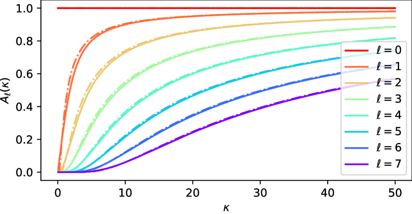
Computing the attenuation function using Equation S8 is inefficient, and it is numerically unstable due to catastrophic cancellation. In Equation 8 of the main paper we present an approximation which is guaranteed to be close to the exact functions from Equation S8, for large values of $\kappa$. We finish this section with a proof of this claim. Additionally, Figure S1 shows that our approximation closely resembles the exact attenuation functions for all values of $\kappa>0$ and all orders $\ell$, and that its quality improves as $\ell$ increases.

Claim 3.

For large values of $\kappa$, our approximation is exact up to an $O(\nicefrac{{1}}{{\kappa^{2}}})$ term, i.e.:

$$A_{\ell}(\kappa)=\exp\left(-\frac{\ell(\ell+1)}{2\kappa}\right)+O\left(\frac{1}{\kappa^{2}}\right)$$ (S15)

Proof.

Using the fact that $\coth(\kappa)=1+O(e^{-2\kappa})$, and using the $i=\ell$ and $i=\ell-1$ terms from the sum in Equation S8 of Claim 2, we have that:

$$A_{\ell}(\kappa)=1-\frac{\ell(\ell+1)}{2\kappa}+O\left(\frac{1}{\kappa^{2}}\right).$$ (S16)

Using a 1st order Taylor approximation for the exponential function yields:

$$\exp\left(-\frac{\ell(\ell+1)}{2\kappa}\right)=1-\frac{\ell(\ell+1)}{2\kappa}+O\left(\frac{1}{\kappa^{2}}\right),$$ (S17)

proving our claim. ∎

Figure S1: The first eight attenuation functions $A_{\ell}(\kappa)$. The exact expression (in solid lines) matches the approximation (in dashed lines), with an increasing accuracy as $\ell$ increases.

Appendix B Interpretations of Normal Vector Penalty

As described in the main paper, the regularization term in Equation 11 penalizes “backwards-facing” normal vectors that contribute to the ray’s final rendered color.

Note that Equation 11 applies this penalty to the normals output by the spatial MLP as opposed to the normal vectors directly computed from the gradient of the density field. While this penalty is remarkably effective at improving recovered normal vectors, we find that directly applying it to the gradient density normals sometimes affects the optimization dynamics for fine geometric structures. Even when NeRF recovers a concentrated surface at the end of optimization, it typically passes through a fuzzier volumetric representation during optimization, and directly penalizing the gradient of the volume density can sometimes adversely affect this trajectory. Our approach of applying the orientation penalty to the predicted normals gives the spatial MLP two options at every location: it can either predict normals that agree with the density gradient ones, in which case our orientation loss is effectively applied to the density field; or it can predict normals that deviate from those computed from the density field, and incur a normal prediction penalty $\mathcal{R}_{p}$. We find that applying the penalty to predicted normals allows our method to adaptively apply the orientation loss, resulting in accurate normals without loss of fine details (see ablation studies).

Besides providing smooth normals for computing reflection directions and providing a mechanism for an adaptive corner-preserving orientation loss, the predicted normals also allow the model to directly encode view directions by predicting a constant normal direction $\hat{\mathbf{n}}^{\prime}(\mathbf{x})=\hat{\mathbf{c}}$, leading to a 1-to-1 mapping from view direction to reflection direction (see Equation 4). While this is discouraged by the normal prediction loss $\mathcal{R}_{p}$, our model can exploit this behavior in regions that are not well-described by a surface at a scale whose geometry the density field can capture.

Appendix C Optimization

Our implementation is based on the official JAX [6] implementation of mip-NeRF [2].

In all of our experiments on synthetic data we apply the normal orientation loss from Equation 11 and the normal prediction loss from Equation 10 of the main paper with weights of $0.1$ and $3\cdot 10^{-4}$ respectively, relative to the standard NeRF data loss from Equation 2. In our experiments on real captured data, we apply a slightly higher weight of $10^{-3}$ on the normal prediction loss. We use the same weights during both the coarse and fine stages.

During training, we add i.i.d. Gaussian noise with standard deviation $0.1$ to the bottleneck $\mathbf{b}$. We find that this slightly stabilizes our model’s results in some cases by preventing it from using the bottleneck early in training.

We optimize all experiments on the Blender scenes using single-image batching to be consistent with results reported in the NeRF and mip-NeRF papers. For our Shiny Blender dataset, we sample random batches of rays from all images.

We train our model, ablations of our model, and all mip-NeRF baselines using a slightly modified version of mip-NeRF’s learning schedule: $250\mathrm{k}$ optimization iterations with a batch size of $2^{14}$, using the Adam [16] optimizer with hyperparameters $\beta_{1}=0.9$, $\beta_{2}=0.999$, $\varepsilon=10^{-6}$, a learning rate that is annealed log-linearly from $2\times 10^{-3}$ to $2\times 10^{-5}$ with a warm-up phase of $512$ iterations, and gradient clipping to a norm of $10^{-3}$.

Appendix D Dataset Details

Our new “Shiny Blender” scenes were adapted from the the following BlendSwap models:

1. Coffee: created by sleem, CC-0 license (model #10827).

2. Toaster: created by PrinterKiller, CC-BY license (model #4989)

3. Car: created by Xali, CC-0 license (model #24359).

4. Helmet: created by kveidem, CC-0 license (model #21617).

Our dataset of real scenes was captured by the authors.

Appendix E Evaluation Details

Normal Vectors

To compute the normal vector for a ray, we sample normals along the ray $\{\hat{\mathbf{n}}_{i}\}$ using Equation 3 from the main paper, and use the volume rendering procedure from Equation 1 to compute a single normal vector:

$$\mathbf{N}(\mathbf{o},\hat{\mathbf{d}})=\sum_{i}w_{i}\hat{\mathbf{n}}(\mathbf{x}_{i}).$$ (S18)

We use Equation S18 to visualize normal maps, with gray-colored values corresponding to high variance normal vectors along a ray. For evaluating MAE, we use the normalized accumulated normals, $\hat{\mathbf{N}}=\mathbf{N}/\|\mathbf{N}\|$.

	sedan	toy car	garden spheres
Mip-NeRF, 8 layers	25.53 / 0.729 / 0.118	24.00 / 0.663 / 0.177	23.40 / 0.620 / 0.125
Ours	25.65 / 0.720 / 0.119	24.25 / 0.674 / 0.168	23.46 / 0.601 / 0.138

Table S1: Quantitative metrics (PSNR/SSIM/LPIPS) on the test sets of our real captured scenes.

Baseline Implementations

For comparisons to mip-NeRF [2], we use the official open-source JAX implementation. For comparisons to PhySG [45], we use the official PyTorch code open-sourced by the authors. However, the original hyperparameters produce poor results on our datasets, so the PhySG authors helped us tune their hyperparameters for the Blender datasets. VolSDF [43] does not currently have publicly-available code, but the authors graciously ran their code on the Blender dataset and provided us with rendered test-set images and normals. We report the NSVF [19] and NeRF [24] results on the Blender dataset from the tables in the mip-NeRF paper.

Appendix F Additional Results

Table S1 reports quantitative metrics on the test sets (every eighth image is held out for testing, as done in NeRF [24]) of our three real captured scenes. Tables S5, S5, S5, and S5 contain quantitative metrics on the original synthetic Blender dataset, and Tables S9, S9, S9, and S9 contain quantitative metrics on our new synthetic Shiny Blender dataset.

	​chair​	​lego​	​materials​	​mic​	​hotdog​	​ficus​	​drums​	​ship​
PhySG [45]	24.00	20.19	18.86	22.33	24.08	19.02	20.99	15.35
VolSDF [43]	30.57	29.46	29.13	30.53	35.11	22.91	20.43	25.51
Mip-NeRF [2]	35.12	35.92	30.64	36.76	37.34	33.19	25.36	30.52
Ours, PE	35.86	36.33	35.22	35.84	38.18	33.60	26.03	30.17
Ours	35.83	36.25	35.41	36.76	37.72	33.91	25.79	30.28

Table S2: Per-scene test set PSNRs on the Blender dataset [24].

	​chair​	​lego​	​materials​	​mic​	​hotdog​	​ficus​	​drums​	​ship​
PhySG [45]	0.898	0.821	0.838	0.933	0.912	0.873	0.884	0.727
VolSDF [43]	0.949	0.951	0.954	0.969	0.972	0.929	0.893	0.842
Mip-NeRF [2]	0.981	0.980	0.959	0.992	0.982	0.980	0.933	0.885
Ours, PE	0.984	0.981	0.983	0.991	0.984	0.982	0.939	0.878
Ours	0.984	0.981	0.983	0.992	0.984	0.983	0.937	0.880

Table S3: Per-scene test set SSIMs on the Blender dataset [24].

	​chair​	​lego​	​materials​	​mic​	​hotdog​	​ficus​	​drums​	​ship​
PhySG [45]	0.093	0.172	0.142	0.082	0.117	0.112	0.113	0.322
VolSDF [43]	0.056	0.054	0.048	0.191	0.043	0.068	0.119	0.191
Mip-NeRF [2]	0.020	0.018	0.040	0.008	0.026	0.021	0.064	0.135
Ours, PE	0.017	0.018	0.023	0.008	0.022	0.020	0.059	0.143
Ours	0.017	0.018	0.022	0.007	0.022	0.019	0.059	0.139

Table S4: Per-scene test set LPIPS on the Blender dataset [24].

	​chair​	​lego​	​materials​	​mic​	​hotdog​	​ficus​	​drums​	​ship​
PhySG [45]	18.569	40.244	18.986	26.053	28.572	35.974	21.696	43.265
VolSDF [43]	14.085	26.619	8.277	19.579	12.170	39.801	21.458	16.974
Mip-NeRF [2]	28.044	30.532	64.074	36.489	29.303	53.524	32.374	37.667
Ours, PE	20.018	26.471	10.162	25.921	13.920	41.557	27.766	34.212
Ours	19.852	24.469	9.531	24.938	13.211	41.052	27.853	31.707

Table S5: Per-scene test set normal MAEs on the Blender dataset [24].

	​teapot​	​toaster​	​car​	​ball​	​coffee​	​helmet​
PhySG [45]	35.83	18.59	24.40	27.24	23.71	27.51
Mip-NeRF [2]	46.00	22.37	26.50	25.94	30.36	27.39
Mip-NeRF, 8 layers	47.35	25.51	27.99	27.53	32.14	29.04
Mip-NeRF, 8 layers, w/ normals	47.09	25.14	27.97	26.79	32.12	29.21
Mip-NeRF, 8 layers, with $\mathcal{R}_{o}$	47.35	25.32	27.91	26.89	32.21	29.22
Ours, no reflection	44.74	24.04	27.41	20.94	31.95	27.76
Ours, no $\mathcal{R}_{o}$	46.80	25.78	28.43	27.06	32.58	29.06
Ours, no pred. normals	47.09	23.32	27.19	26.09	31.79	30.54
Ours, concat. viewdir	46.01	25.38	30.71	47.45	34.19	28.81
Ours, fixed lobe	46.82	25.57	30.09	47.25	34.37	29.00
Ours, no diffuse color	46.45	25.56	30.46	34.53	34.05	28.87
Ours, no tint	46.54	25.49	30.14	47.53	34.24	28.78
Ours, no roughness	45.28	25.39	30.44	36.33	33.19	29.72
Ours, PE	46.55	26.74	30.53	47.56	34.45	29.59
Ours	47.90	25.70	30.82	47.46	34.21	29.68

Table S6: Per-scene test set PSNRs on our Shiny Blender dataset.

	​teapot​	​toaster​	​car​	​ball​	​coffee​	​helmet​
PhySG [45]	0.990	0.805	0.910	0.947	0.922	0.953
Mip-NeRF [2]	0.997	0.891	0.922	0.935	0.966	0.939
Mip-NeRF, 8 layers	0.997	0.925	0.936	0.949	0.971	0.957
Mip-NeRF, 8 layers, w/ normals	0.997	0.923	0.936	0.946	0.970	0.957
Mip-NeRF, 8 layers, with $\mathcal{R}_{o}$	0.997	0.924	0.935	0.947	0.971	0.957
Ours, no reflection	0.996	0.912	0.930	0.905	0.970	0.950
Ours, no $\mathcal{R}_{o}$	0.997	0.926	0.937	0.939	0.971	0.956
Ours, no pred. normals	0.997	0.898	0.926	0.865	0.967	0.962
Ours, concat. viewdir	0.997	0.919	0.956	0.995	0.974	0.952
Ours, fixed lobe	0.997	0.920	0.952	0.995	0.974	0.954
Ours, no diffuse color	0.997	0.920	0.953	0.977	0.973	0.954
Ours, no tint	0.997	0.921	0.951	0.995	0.974	0.954
Ours, no roughness	0.996	0.917	0.954	0.983	0.972	0.958
Ours, PE	0.997	0.928	0.954	0.996	0.975	0.958
Ours	0.998	0.922	0.955	0.995	0.974	0.958

Table S7: Per-scene test set SSIMs on our Shiny Blender dataset.

	​teapot​	​toaster​	​car​	​ball​	​coffee​	​helmet​
PhySG [45]	0.022	0.194	0.091	0.179	0.150	0.089
Mip-NeRF [2]	0.008	0.123	0.059	0.168	0.086	0.108
Mip-NeRF, 8 layers	0.006	0.080	0.052	0.139	0.082	0.072
Mip-NeRF, 8 layers, w/ normals	0.006	0.085	0.052	0.144	0.082	0.072
Mip-NeRF, 8 layers, with $\mathcal{R}_{o}$	0.006	0.082	0.052	0.143	0.082	0.072
Ours, no reflection	0.007	0.091	0.052	0.192	0.082	0.080
Ours, no $\mathcal{R}_{o}$	0.008	0.086	0.051	0.161	0.082	0.076
Ours, no pred. normals	0.006	0.134	0.064	0.272	0.087	0.068
Ours, concat. viewdir	0.006	0.095	0.040	0.061	0.079	0.087
Ours, fixed lobe	0.009	0.096	0.043	0.061	0.080	0.080
Ours, no diffuse color	0.009	0.096	0.043	0.095	0.079	0.080
Ours, no tint	0.008	0.094	0.043	0.060	0.079	0.078
Ours, no roughness	0.009	0.099	0.042	0.086	0.081	0.074
Ours, PE	0.007	0.092	0.041	0.060	0.077	0.074
Ours	0.004	0.095	0.041	0.059	0.078	0.075

Table S8: Per-scene test set LPIPS on our Shiny Blender dataset.

	​teapot​	​toaster​	​car​	​ball​	​coffee​	​helmet​
PhySG [45]	6.634	9.749	8.844	0.700	22.514	2.324
Mip-NeRF [2]	66.470	42.787	40.954	104.765	29.427	77.904
Mip-NeRF, 8 layers	68.238	35.220	23.670	127.863	25.465	67.966
Mip-NeRF, 8 layers, w/ normals	67.999	34.093	23.548	130.755	26.527	66.701
Mip-NeRF, 8 layers, with $\mathcal{R}_{o}$	68.238	35.837	23.985	127.683	24.101	64.372
Ours, no reflection	19.263	19.325	13.643	15.142	9.730	20.038
Ours, no $\mathcal{R}_{o}$	43.116	43.113	37.134	106.003	29.301	56.710
Ours, no pred. normals	67.999	24.886	21.644	48.061	10.848	10.573
Ours, concat. viewdir	20.359	40.587	12.877	1.577	9.489	42.615
Ours, fixed lobe	35.791	42.183	18.410	1.536	24.045	36.785
Ours, no diffuse color	38.347	42.705	16.802	5.423	15.363	38.119
Ours, no tint	29.537	43.687	16.854	1.556	11.233	33.327
Ours, no roughness	33.821	44.666	17.440	3.557	26.578	29.723
Ours, PE	23.123	41.415	16.214	1.969	9.749	29.409
Ours	9.234	42.870	14.927	1.548	12.240	29.484

Table S9: Per-scene test set MAEs on our Shiny Blender dataset.

References

- [1] Matthew Anderson, Ricardo Motta, Srinivasan Chandrasekar, and Michael Stokes. Proposal for a standard default color space for the internet—sRGB. Color and imaging conference, 1996.
- [2] Jonathan T. Barron, Ben Mildenhall, Matthew Tancik, Peter Hedman, Ricardo Martin-Brualla, and Pratul P. Srinivasan. Mip-NeRF: A multiscale representation for anti-aliasing neural radiance fields. ICCV, 2021.
- [3] Sai Bi, Zexiang Xu, Pratul P. Srinivasan, Ben Mildenhall, Kalyan Sunkavalli, Milos Hasan, Yannick Hold-Geoffroy, David Kriegman, and Ravi Ramamoorthi. Neural reflectance fields for appearance acquisition. arXiv, 2020.
- [4] Mark Boss, Raphael Braun, Varun Jampani, Jonathan T. Barron, Ce Liu, and Hendrik P. A. Lensch. NeRD: Neural reflectance decomposition from image collections. ICCV, 2021.
- [5] Mark Boss, Varun Jampani, Raphael Braun, Ce Liu, Jonathan T. Barron, and Hendrik P. A. Lensch. Neural-PIL: Neural pre-integrated lighting for reflectance decomposition. NeurIPS, 2021.
- [6] James Bradbury, Roy Frostig, Peter Hawkins, Matthew James Johnson, Chris Leary, Dougal Maclaurin, George Necula, Adam Paszke, Jake VanderPlas, Skye Wanderman-Milne, and Qiao Zhang. JAX: composable transformations of Python+NumPy programs, 2018. http://github.com/google/jax.
- [7] Chris Buehler, Michael Bosse, Leonard McMillan, Steven Gortler, and Michael Cohen. Unstructured lumigraph rendering. SIGGRAPH, 2001.
- [8] Shenchang Eric Chen and Lance Williams. View interpolation for image synthesis. SIGGRAPH, 1993.
- [9] Paul E. Debevec, Camillo J. Taylor, and Jitendra Malik. Modeling and rendering architecture from photographs: a hybrid geometry-and image-based approach. SIGGRAPH, 1996.
- [10] John Flynn, Michael Broxton, Paul Debevec, Matthew DuVall, Graham Fyffe, Ryan Overbeck, Noah Snavely, and Richard Tucker. DeepView: View synthesis with learned gradient descent. CVPR, 2019.
- [11] Guy Gafni, Justus Thies, Michael Zollhöfer, and Matthias Nießner. Dynamic neural radiance fields for monocular 4D facial avatar reconstruction. CVPR, 2021.
- [12] Steven J. Gortler, Radek Grzeszczuk, Richard Szeliski, and Michael F. Cohen. The lumigraph. SIGGRAPH, 1996.
- [13] Peter Hedman, Julien Philip, True Price, Jan-Michael Frahm, George Drettakis, and Gabriel Brostow. Deep blending for free-viewpoint image-based rendering. ACM Transactions on Graphics (SIGGRAPH Asia), 2018.
- [14] Peter Hedman, Pratul P. Srinivasan, Ben Mildenhall, Jonathan T. Barron, and Paul Debevec. Baking neural radiance fields for real-time view synthesis. ICCV, 2021.
- [15] Jan Kautz and Michael D. McCool. Approximation of glossy reflection with prefiltered environment maps. Graphics Interface, 2000.
- [16] Diederik P. Kingma and Jimmy Ba. Adam: A method for stochastic optimization. ICLR, 2015.
- [17] Johannes Kopf, Fabian Langguth, Daniel Scharstein, Richard Szeliski, and Michael Goesele. Image-based rendering in the gradient domain. ACM Transactions on Graphics (SIGGRAPH Asia), 2013.
- [18] Marc Levoy and Pat Hanrahan. Light field rendering. SIGGRAPH, 1996.
- [19] Lingjie Liu, Jiatao Gu, Kyaw Zaw Lin, Tat-Seng Chua, and Christian Theobalt. Neural sparse voxel fields. NeurIPS, 2020.
- [20] Stephen Lombardi, Tomas Simon, Jason Saragih, Gabriel Schwartz, Andreas Lehrmann, and Yaser Sheikh. Neural volumes: Learning dynamic renderable volumes from images. ACM Transactions on Graphics (SIGGRAPH), 2019.
- [21] Ricardo Martin-Brualla, Noha Radwan, Mehdi S. M. Sajjadi, Jonathan T. Barron, Alexey Dosovitskiy, and Daniel Duckworth. NeRF in the wild: Neural radiance fields for unconstrained photo collections. CVPR, 2021.
- [22] Nelson Max. Optical models for direct volume rendering. IEEE TVCG, 1995.
- [23] Ben Mildenhall, Pratul P. Srinivasan, Rodrigo Ortiz-Cayon, Nima Khademi Kalantari, Ravi Ramamoorthi, Ren Ng, and Abhishek Kar. Local light field fusion: Practical view synthesis with prescriptive sampling guidelines. ACM Transactions on Graphics (SIGGRAPH), 2019.
- [24] Ben Mildenhall, Pratul P. Srinivasan, Matthew Tancik, Jonathan T. Barron, Ravi Ramamoorthi, and Ren Ng. NeRF: Representing scenes as neural radiance fields for view synthesis. ECCV, 2020.
- [25] Michael Oechsle, Songyou Peng, and Andreas Geiger. UNISURF: Unifying neural implicit surfaces and radiance fields for multi-view reconstruction. ICCV, 2021.
- [26] Keunhong Park, Utkarsh Sinha, Jonathan T. Barron, Sofien Bouaziz, Dan B. Goldman, Steven M. Seitz, and Ricardo Martin-Brualla. Nerfies: Deformable neural radiance fields. ICCV, 2021.
- [27] Sida Peng, Junting Dong, Qianqian Wang, Shangzhan Zhang, Qing Shuai, Xiaowei Zhou, and Hujun Bao. Animatable neural radiance fields for modeling dynamic human bodies. ICCV, 2021.
- [28] Bui Tuong Phong. Illumination for computer generated pictures. Communications of the ACM, 1975.
- [29] Ravi Ramamoorthi. Precomputation-based rendering. Foundations and Trends in Computer Graphics and Vision, 2009.
- [30] Ravi Ramamoorthi and Pat Hanrahan. A signal-processing framework for inverse rendering. SIGGRAPH, 2001.
- [31] Ravi Ramamoorthi and Pat Hanrahan. Frequency space environment map rendering. SIGGRAPH, 2002.
- [32] Gernot Riegler and Vladlen Koltun. Free view synthesis. ECCV, 2020.
- [33] Simon Rodriguez, Siddhant Prakash, Peter Hedman, and George Drettakis. Image-based rendering of cars using semantic labels and approximate reflection flow. Proc. ACM Comput. Graph. Interact. Tech., 2020.
- [34] Szymon M. Rusinkiewicz. A new change of variables for efficient BRDF representation. Eurographics Rendering Workshop, 1998.
- [35] Sudipta N. Sinha, Johannes Kopf, Michael Goesele, Daniel Scharstein, and Richard Szeliski. Image-based rendering for scenes with reflections. ACM Transactions on Graphics (SIGGRAPH), 2012.
- [36] Pratul P. Srinivasan, Boyang Deng, Xiuming Zhang, Matthew Tancik, Ben Mildenhall, and Jonathan T. Barron. NeRV: Neural reflectance and visibility fields for relighting and view synthesis. CVPR, 2021.
- [37] Pratul P. Srinivasan, Richard Tucker Joand nathan T. Barron, Ravi Ramamoorthi, Ren Ng, and Noah Snavely. Pushing the boundaries of view extrapolation with multiplane images. CVPR, 2019.
- [38] Matthew Tancik, Pratul P. Srinivasan, Ben Mildenhall, Sara Fridovich-Keil, Nithin Raghavan, Utkarsh Singhal, Ravi Ramamoorthi, Jonathan T. Barron, and Ren Ng. Fourier features let networks learn high frequency functions in low dimensional domains. NeurIPS, 2020.
- [39] Peng Wang, Lingjie Liu, Yuan Liu, Christian Theobalt, Taku Komura, and Wenping Wang. NeuS: Learning neural implicit surfaces by volume rendering for multi-view reconstruction. NeurIPS, 2021.
- [40] Zhou Wang, Alan C. Bovik, Hamid R. Sheikh, and Eero P. Simoncelli. Image quality assessment: from error visibility to structural similarity. IEEE TIP, 2004.
- [41] Suttisak Wizadwongsa, Pakkapon Phongthawee, Jiraphon Yenphraphai, and Supasorn Suwajanakorn. NeX: Real-time view synthesis with neural basis expansion. CVPR, 2021.
- [42] Daniel Wood, Daniel Azuma, Wyvern Aldinger, Brian Curless, Tom Duchamp, David Salesin, and Werner Stuetzle. Surface light fields for 3D photography. SIGGRAPH, 2000.
- [43] Lior Yariv, Jiatao Gu, Yoni Kasten, and Yaron Lipman. Volume rendering of neural implicit surfaces. NeurIPS, 2021.
- [44] Lior Yariv, Yoni Kasten, Dror Moran, Meirav Galun, Matan Atzmon, Ronen Basri, and Yaron Lipman. Multiview neural surface reconstruction by disentangling geometry and appearance. NeurIPS, 2020.
- [45] Kai Zhang, Fujun Luan, Qianqian Wang, Kavita Bala, and Noah Snavely. PhySG: Inverse rendering with spherical gaussians for physics-based material editing and relighting. CVPR, 2021.
- [46] Richard Zhang, Phillip Isola, Alexei A. Efros, Eli Shechtman, and Oliver Wang. The unreasonable effectiveness of deep features as a perceptual metric. CVPR, 2018.
- [47] Xiuming Zhang, Pratul P. Srinivasan, Boyang Deng, Paul Debevec, William T. Freeman, and Jonathan T. Barron. NeRFactor: Neural factorization of shape and reflectance under an unknown illumination. ACM Transactions on Graphics (SIGGRAPH Asia), 2021.
- [48] Tinghui Zhou, Richard Tucker, John Flynn, Graham Fyffe, and Noah Snavely. Stereo magnification: Learning view synthesis using multiplane images. ACM Transactions on Graphics (SIGGRAPH), 2018.