Grounded Language-Image Pre-training

Abstract

This paper presents a grounded language-image pre-training (GLIP) model for learning object-level, language-aware, and semantic-rich visual representations. GLIP unifies object detection and phrase grounding for pre-training. The unification brings two benefits: 1) it allows GLIP to learn from both detection and grounding data to improve both tasks and bootstrap a good grounding model; 2) GLIP can leverage massive image-text pairs by generating grounding boxes in a self-training fashion, making the learned representations semantic-rich. In our experiments, we pre-train GLIP on 27M grounding data, including 3M human-annotated and 24M web-crawled image-text pairs. The learned representations demonstrate strong zero-shot and few-shot transferability to various object-level recognition tasks. 1) When directly evaluated on COCO and LVIS (without seeing any images in COCO during pre-training), GLIP achieves 49.8 AP and 26.9 AP, respectively, surpassing many supervised baselines. 2) After fine-tuned on COCO, GLIP achieves 60.8 AP on val and 61.5 AP on test-dev, surpassing prior SoTA. 3) When transferred to 13 downstream object detection tasks, a 1-shot GLIP rivals with a fully-supervised Dynamic Head. Code is released at https://github.com/microsoft/GLIP.

1 Introduction

Visual recognition models are typically trained to predict a fixed set of pre-determined object categories, which limits their usability in real-world applications since additional labeled data are needed to generalize to new visual concepts and domains. CLIP [45] shows that image-level visual representations can be learned effectively on large amounts of raw image-text pairs. Because the paired texts contain a boarder set of visual concepts than any pre-defined concept pool, the pre-trained CLIP model is so semantically rich that it can be easily transferred to downstream image classification and text-image retrieval tasks in zero-shot settings. However, to gain fine-grained understanding of images, as required by many tasks, such as object detection [49, 36], segmentation [40, 7], human pose estimation [63, 54], scene understanding [30, 64, 16], action recognition [20], vision-language understanding [41, 55, 8, 53, 33, 32, 73, 35, 34, 70], object-level visual representations are highly desired.

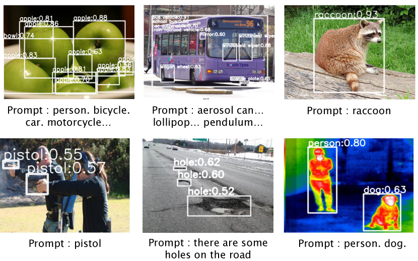
Figure 1: GLIP zero-shot transfers to various detection tasks, by writing the categories of interest into a text prompt.

In this paper, we show that phrase grounding, which is a task of identifying the fine-grained correspondence between phrases in a sentence and objects (or regions) in an image, is an effective and scalable pre-training task to learn an object-level, language-aware, and semantic-rich visual representation, and propose Grounded Language-Image Pre-training (GLIP). Our approach unifies the phrase grounding and object detection tasks in that object detection can be cast as context-free phrase grounding while phrase grounding can be viewed as a contextualized object detection task. We highlight our key contributions as follows.

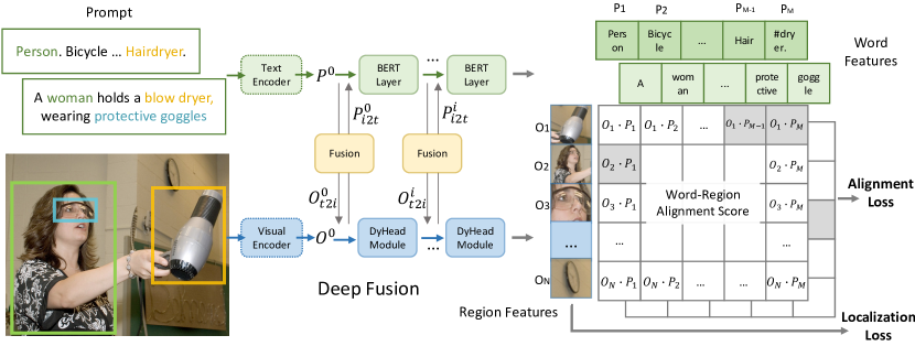
[1.58] [0.42]

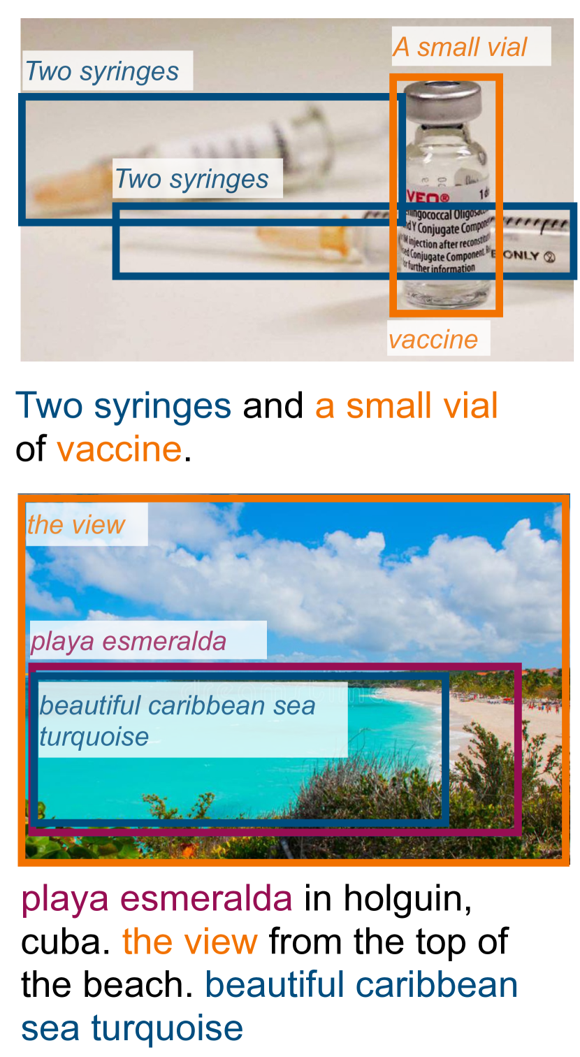
Figure 2: A unified framework for detection and grounding. Unlike a classical object detection model which predicts a categorical class for each detected object, we reformulate detection as a grounding task by aligning each region/box to phrases in a text prompt. GLIP jointly trains an image encoder and a language encoder to predict the correct pairings of regions and words. We further add the cross-modality deep fusion to early fuse information from two modalities and to learn a language-aware visual representation.

Figure 3: Grounding predictions from GLIP. GLIP can locate rare entities, phrases with attributes, and even abstract words.

Unifying detection and grounding by reformulating object detection as phrase grounding. The reformulation changes the input of a detection model: it takes as input not only an image but also a text prompt that describes all the candidate categories in the detection task. For example, the text prompt for COCO object detection [37] is a text string that consists of 80 phrases, i.e., the 80 COCO object class names, joined by “. ”, as shown in Figure 3 (Left). Any object detection model can be converted to a grounding model by replacing the object classification logits in its box classifier with the word-region alignment scores, i.e., dot product of the region (or box) visual features and the token (or phrase) language features, as shown in Figure 3 (Right). The language features are computed using a language model, which gives the new detection (or grounding) model a dual-encoder structure. Different from CLIP that fuses vision and language only at the last dot product layer [45], we show that deep cross-modality fusion applied by GLIP, as shown in Figure 3 (Middle), is crucial to learn high-quality language-aware visual representations and to achieve superior transfer learning performance. The unification of detection and grounding also allows us to pre-train using both types of data and benefits both tasks. On the detection side, the pool of visual concepts is significantly enriched thanks to the grounding data. On the grounding side, detection data introduce more bounding box annotations and help train a new SoTA phrase grounding model.

Scaling up visual concepts with massive image-text data. Given a good grounding model (teacher), we can augment GLIP pre-training data by automatically generating grounding boxes for massive image-text-paired data, in which noun phrases are detected by an NLP parser [2]. Thus, we can pre-train our (student) GLIP-Large model (GLIP-L) on 27M grounding data, including 3M human-annotated fine-grained data and 24M web-crawled image-text pairs. For the 24M image-text pairs, there are 78.1M high-confidence ($>0.5$) phrase-box pseudo annotations, with 58.4M unique noun phrases. We showcase two real examples of the generated boxes in Figure 3. The teacher model can accurately localize some arguably hard concepts, such as syringes, vaccine, beautiful caribbean sea turquoise, and even abstract words (the view). Training on such semantic-rich data delivers a semantic-rich student model. In contrast, prior work on scaling detection data simply cannot predict concepts out of the teacher models’ pre-defined vocabulary [77]. In this study, we show that this simple strategy of scaling up grounding data is empirically effective, bringing large improvements to LVIS and 13 downstream detection tasks, especially on rare categories (Sections 4.2 and 5). When the pre-trained GLIP-L model is fine-tuned on COCO, it achieves 60.8 AP on COCO 2017val and 61.5 on test-dev, surpassing the current public SoTA models [10, 65] that scale up object detection data in various approaches.

Transfer learning with GLIP: one model for all. The grounding reformulation and semantic-rich pre-training facilitate domain transfer. GLIP can be transferred to various tasks with few or even no additional human annotations. When the GLIP-L model is directly evaluated on the COCO and LVIS datasets (without seeing any images in COCO during pre-training), it achieves 49.8 and 26.9 AP on COCO val2017 and LVIS val, respectively, surpassing many supervised baselines. When evaluated on 13 existing object detection datasets, spanning scenarios including fine-grained species detection, drone-view detection, and ego-centric detection, the setting which we term “Object Detection in the Wild” (ODinW) (Section 5.1), GLIP exhibits excellent data efficiency. For example, a zero-shot GLIP-L outperforms a 10-shot supervised baseline (Dynamic Head) pre-trained on Objects365 while a 1-shot GLIP-L rivals with a fully supervised Dynamic Head. Moreover, when task-specific annotations are available, instead of tuning the whole model, one could tune only the task-specific prompt embedding, while keeping the model parameters unchanged. Under such a prompt tuning setting (Section 5.2), one GLIP model can simultaneously perform well on all downstream tasks , reducing the fine-tuning and deployment cost.

2 Related Work

Standard object detection systems are trained to localize a fixed set of object classes predefined in crowd-labeled datasets, such as COCO [37], OpenImages (OI) [30], Objects365 [50], and Visual Genome (VG) [28], which contains no more than 2,000 object classes. Such human-annotated data are costly to scale up [59]. GLIP presents an affordable solution by reformulating object detection as a phrase grounding (word-to-region matching) problem, and thus enables the use of grounding and massive image-text-paired data. Though our current implementation is built upon Dynamic Head (DyHead) [10], our unified formulation can be generalized to any object detection systems  [48, 36, 10, 9, 49, 6, 4, 76, 10].

Recently, there is a trend to develop vision-and-language approaches to visual recognition problems, where vision models are trained with free-form language supervision. For example, CLIP [45] and ALIGN [21] perform cross-modal contrastive learning on hundreds or thousands of millions of image-text pairs and can directly perform open-vocabulary image classification. By distilling the knowledge from the CLIP/ALIGN model into a two-stage detector, ViLD [14] is proposed to advance zero-shot object detection. Alternatively, MDETR [23] trains an end-to-end model on existing multi-modal datasets which have explicit alignment between phrases in text and objects in image. Our GLIP inherits the semantic-rich and language-aware property of this line of research, achieves SoTA object detection performance and significantly improves the transferability to downstream detection tasks.

This paper focuses on domain transfer for object detection. The goal is to build one pre-trained model that seamlessly transfers to various tasks and domains, in a zero-shot or few-shot manner. Our setting differs from zero-shot detection [1, 47, 12, 68, 14, 46], where some categories are defined as unseen/rare and not present in the training set. We expect GLIP to perform well on rare categories (Section 4.2) but we do not explicitly exclude any categories from our training set, because grounding data are so semantically rich that we expect them to cover many rare categories. This resembles the setting in open-vocabulary object detection [68], which expects raw image-text data to cover many rare categories. A line of work identifies building a open-world object proposal module that could propose any novel object at test time as the key challenge [74, 75, 60, 22, 25]; GLIP offers a new perspective: the model does not need to propose every possible novel objects from an open set; rather it only needs to propose objects mentioned in the text prompt as the detection branch is conditioned on the prompt.

Beyond performance on rare categories, we also consider the transfer cost in real-world scenarios, i.e., how to achieve the best performance with the least amount of data, training budget, and deployment cost (Section 5). In particular, we show that GLIP supports prompt tuning [31], which matches the performance of full fine-tuning but only tunes a fraction of the model parameters. We also present a novel finding that in object detection, prompt tuning is most effective for a model with deep vision-language fusion such as GLIP, while being far less effective for shallow-fused models. This stands in contrast to recent work that investigates prompt tuning only for shallow-fused vision-language models such as CLIP  [72, 13, 71].

3 Grounded Language Image Pre-training

Conceptually, object detection and phrase grounding bear a great similarity. They both seek to localize objects and align them to semantic concepts. This synergy motivates us to cast the classical object detection task into a grounding problem and propose a unified formulation (Sec 3.1). We further propose to add deep fusion between image and text, making the detection model language-aware and thus a strong grounding model (Sec 3.2). With the reformulation and deep fusion, we can pre-train GLIP on scalable and semantic-rich grounding data (Sec 3.3).

3.1 Unified Formulation

Background: object detection. A typical detection model feeds an input image into a visual encoder $\text{Enc}_{I}$, with CNN [18, 56] or Transformer [39, 69, 67] as backbone, and extracts region/box features $O$, as shown in Figure 3 (Bottom). Each region/box feature is fed into two prediction heads, i.e., a box classifier $\mathcal{C}$ and a box regressor $\mathcal{R}$, which are trained with the classification loss $\mathcal{L}_{\text{cls}}$ and the localization loss $\mathcal{L}_{\text{loc}}$, respectively:

$$\mathcal{L}=\mathcal{L}_{\text{cls}}+\mathcal{L}_{\text{loc}}.$$ (1)

In two-stage detectors, a separate region proposal network (RPN) with RPN loss $\mathcal{L}_{\text{rpn}}$ is used to distinguish foreground from background and refine anchors. Since $\mathcal{L}_{\text{rpn}}$ does not use semantic information of object classes, we merge it into the localization loss $\mathcal{L}_{\text{loc}}$. In one-stage detectors, localization loss $\mathcal{L}_{\text{loc}}$ may also contain the centerness loss [57].

The box classifier $\mathcal{C}$ is typically a simple linear layer, and the classification loss $\mathcal{L}_{\text{cls}}$ can be written as:

$$O\!=\!\text{Enc}_{I}(\text{Img}),\ S_{\text{cls}}\!=\!OW^{T},\ \mathcal{L}_{\text{cls}}\!=\!loss(S_{\text{cls}};T).$$ (2)

Here, $O\in\mathbb{R}^{N\times d}$ are the object/region/box features of the input image, $W\in\mathbb{R}^{c\times d}$ is the weight matrix of the box classifier $\mathcal{C}$, $S_{\text{cls}}\in\mathbb{R}^{N\times c}$ are the output classification logits, $T\in\{0,1\}^{N\times c}$ is the target matching between regions and classes computed from the classical many-to-1 matching [48, 36, 9, 49] or the bipartite Hungarian match [4, 76, 10]. $loss(S;T)$ is typically a cross-entropy loss for two-stage detectors and a focal loss [36] for one-stage detectors.

Object detection as phrase grounding. Instead of classifying each region/box into $c$ classes, we reformulate detection as a grounding task, by grounding/aligning each region to $c$ phrases in a text prompt (see Figure 3). How to design a text prompt for a detection task? Given object classes $[\text{person, bicycle, car, ..., toothbrush}]$, one simple way is

$$\text{Prompt}=\text{``Detect: person, bicycle, car, ... , toothbrush''},$$

in which each class name is a candidate phrase to be grounded. One could design better prompts, by providing more expressive descriptions of these classes and/or by exploiting the preference of a pre-trained language model. For example, when the pre-trained BERT model [11] is used to initialize our language encoder $\text{Enc}_{L}$, the prompt “person. bicycle. car. … . toothbrush” works better than the more human-friendly prompt described above. We will discuss the prompt design in Section 5.2.

In a grounding model, we compute the alignment scores $S_{\text{ground}}$ between image regions and words in the prompt:

$$O\!=\!\text{Enc}_{I}(\text{Img}),~{}P\!=\!\text{Enc}_{L}(\text{Prompt}),~{}S_{\text{ground}}\!=\!OP^{\top},$$ (3)

where $P\in\mathbb{R}^{M\times d}$ is the contextual word/token features from the language encoder and plays a similar role to the weight matrix $W$ in (2), as shown in Figure 3 (Right). The grounding model, consisting of both the image encoder $\text{Enc}_{I}$ and the language encoder $\text{Enc}_{L}$, is trained end-to-end by minimizing the loss defined in (1) & (2), with a simple replacement of the classification logits $S_{\text{cls}}$ in (2) with the region-word aligment scores $S_{\text{ground}}$ in (3).

However, in (2), we now have the logits $S_{\text{ground}}\in\mathbb{R}^{N\times M}$ and the target $T\in\{0,1\}^{N\times c}$. The number of (sub)-word tokens $M$ is always larger than the number of phrases $c$ in the text prompt due to four reasons: 1) some phrases contain multiple words, e.g., “traffic light”; 2) some single-word phrases are splitted into multiple (sub)-word tokens, e.g., “toothbrush” to “tooth#” and “#brush”; 3) some are the added tokens, such as “Detect:”, “,”, special tokens in language models, and 4) a [NoObj] token is added at the end of the tokenized sequence. When the $loss$ is a (focal) binary sigmoid loss (the $loss$ we use in Section 4 & 5), we expand the original target matrix $T\in\{0,1\}^{N\times c}$ to $T^{\prime}\in\{0,1\}^{N\times M}$ by making all sub-words positive match if a phrase is a positive match and all added tokens negative match to all image features. With this change, the $loss(S_{\text{ground}};T^{\prime})$ remains the same. During inference, we average token probabilities as the phrase probability.

Equivalence between detection and grounding. With the above reformulation, we can convert any detection model into a grounding model, and the two views, i.e., detection and grounding, are theoretically equivalent for both training and inference. We also verify this empirically: the SoTA DyHead detector [10] with Swin-Tiny backbone gives the same performance on COCO val2017 before and after our reformulation. Please refer to the appendix for discussions. With the reformulation, a pre-trained phrase grounding model can be directly applied to any object detection task, thanks to the free-form input of the language encoder. This makes it possible to transfer our GLIP model to arbitrary detection tasks in a zero-shot manner.

Related work. Our grounding formulation is inspired by MDETR [23], and our grounding loss shares the same spirit of MDETR’s fine-grained contrastive loss. We go further than MDETR by finding an effective approach to reformulate detection as grounding and a simple unified loss for both detection and grounding tasks. Our grounding model also resembles models for zero-shot detection [1, 47, 14, 75, 46]. The seminal work of Bansal et al. [1] enables a detection model to conduct zero-shot detection, by using the pre-trained Glove word embedding [43] as the phrase features $P\in\mathbb{R}^{c\times d}$, if written in the form of (3). Recently, phrase features extracted from pre-trained deep language models are introduced in open-vocabulary detection [68]. GLIP differs from zero-shot detection in that GLIP provides a unified view of detection and grounding, and enables two crucial ingredients, i.e., language-aware deep fusion and scaling up with image-text data, as to be described next.

3.2 Language-Aware Deep Fusion

In (3), the image and text are encoded by separate encoders and only fused at the end to calculate the alignment scores. We call such models late-fusion models. In vision-language literature [41, 55, 8, 53, 33, 32, 73, 35, 23], deep fusion of visual and language features is necessary to learn a performant phrase grounding model. We introduce deep fusion between the image and language encoders, which fuses the image and text information in the last few encoding layers, as shown in Figure 3 (Middle). Concretely, when we use DyHead [10] as the image encoder and BERT [11] as the text encoder, the deep-fused encoder is:

$${\color[rgb]{1,0,0}O^{i}_{\text{t2i}},P^{i}_{\text{i2t}}}=\text{X-MHA}(O^{i},P^{i}),\quad i\in\{0,1,..,L-1\}$$ (4)

$$O^{i+1}=\text{DyHeadModule}(O^{i}{\color[rgb]{1,0,0}+O^{i}_{\text{t2i}}}),\quad O=O^{L},$$ (5)

$$P^{i+1}=\text{BERTLayer}(P^{i}{\color[rgb]{1,0,0}+P^{i}_{\text{i2t}}}),\quad P=P^{L},$$ (6)

where $L$ is the number of DyHeadModules in DyHead [10], BERTLayer is newly-added BERT Layers on top of the pre-trained BERT, $O^{0}$ denote the visual features from the vision backbone, and $P^{0}$ denote the token features from the language backbone (BERT). The cross-modality communication is achieved by the cross-modality multi-head attention module (X-MHA) (4), followed by the single modality fusion and updated in (5) & (6). Without added context vectors ($O^{i}_{\text{t2i}}$ for vision modality and $P^{i}_{\text{i2t}}$ for language modality), the model is reduced to a late-fusion model.

In the cross-modality multi-head attention module (X-MHA) (4), each head computes the context vectors of one modality by attending to the other modality:

$$O^{(q)}\!=\!OW^{(q,I)},P^{(q)}\!=\!PW^{(q,L)},Attn\!=\!O^{(q)}(P^{(q)})^{\top}\!/\!\sqrt{d},$$

$$P^{(v)}=PW^{(v,L)},~{}~{}O_{\text{t2i}}=\text{SoftMax}(Attn)P^{(v)}W^{(out,I)},$$

$$O^{(v)}=OW^{(v,I)},~{}~{}P_{\text{i2t}}=\text{SoftMax}(Attn^{\top})O^{(v)}W^{(out,L)},$$

where $\{W^{(\text{symbol},I)},W^{(\text{symbol},L)}:\text{symbol}\in\{q,v,out\}\}$ are trainable parameters and play similar roles to those of query, value, and output linear layers in Multi-Head Self-Attention [58], respectively.

The deep-fused encoder (4)-(6) brings two benefits. 1) It improves the phrase grounding performance. 2) It makes the learned visual features language-aware, and thus the model’s prediction is conditioned on the text prompt. This is crucial to achieve the goal of having one model serve all downstream detection tasks (shown in Section 5.2).

3.3 Pre-training with Scalable Semantic-Rich Data

Considerable efforts have been devoted to collecting detection data that are rich in semantics and large in quantity. However, human annotations have been proven costy and limited [30, 15]. Prior work seeks to scale up in a self-training fashion [77]. They use a teacher (a pre-trained detector) to predict boxes from raw images and generate pseudo detection labels to train a student model. But the generated data are still limited in terms of the size of the concept pool, as the teacher can only predict labels defined in the concept pool, constructed on the existing datasets. In contrast, our model can be trained on both detection and, more importantly, grounding data. We show that grounding data can provide rich semantics to facilitate localization and can be scaled up in a self-training fashion.

First, the gold grounding data cover a much larger vocabulary of visual concepts than existing detection data. The largest attempts at scaling up detection vocabulary still cover no more than 2,000 categories [28, 15]. With grounding data, we expand the vocabulary to cover virtually any concepts that appear in the grounded captions. For example, Flickr30K [44] contains 44,518 unique phrases while VG Caption [28] contains 110,689 unique phrases, orders of magnitude larger than the vocabulary of detection data. We provide an empirical study in Section 4.4 to show that 0.8M gold grounding data brings a larger improvement on detecting rare categories than additional 2M detection data.

Further, instead of scaling up detection data, we show a promising route to obtaining semantically rich data: scaling up grounding data. We use a simple approach inspired by self-training. We first pre-train a teacher GLIP with gold (human-annotated) detection and grounding data. Then we use this teacher model to predict boxes for web-collected image-text data, with noun phrases detected by an NLP parser [2]. Finally, a student model is trained with both the gold data and the generated pseudo grounding data. As shown in Figure 3, the teacher is capable of generating accurate boxes for semantically rich entities.

Why can the student model possibly outperform the teacher model? While discussions remain active in the self-training literature [77], in the context of visual grounding, we posit that the teacher model is utilizing the language context and language generalization ability to accurately ground concepts that it may not inherently know. For example, in Figure 3, the teacher may not directly recognize certain concepts such as vaccine and turquoise, if they are not present in gold data. However, the rich language context such as syntactic structures can provide strong guidance for the teacher model to perform an “educated guess”. The model can localize vaccine if it can localize a small vail; it can localize turquoise if it can find caribbean sea. When we train the student model, the “educated guess” of the teacher model becomes a “supervised signal”, enabling the student model to learn the concept of vaccine and turquoise.

Table 1: A detailed list of GLIP model variants.

Model	Backbone	Deep Fusion	Pre-Train Data
			Detection	Grounding	Caption
GLIP-T (A)	Swin-T	✗	Objects365	-	-
GLIP-T (B)	Swin-T	✓	Objects365	-	-
GLIP-T (C)	Swin-T	✓	Objects365	GoldG	-
GLIP-T	Swin-T	✓	Objects365	GoldG	Cap4M
GLIP-L	Swin-L	✓	FourODs	GoldG	Cap24M

4 Transfer to Established Benchmarks

Table 2: Zero-shot domain transfer and fine-tuning on COCO. GLIP, without seeing any images from the COCO dataset, can achieve comparable or superior performance than prior supervised models (e.g. GLIP-T under Zero-Shot v.s. Faster RCNN under Fine-Tune). When fully fine-tuned on COCO, GLIP-L surpasses the SoTA performance.

Model	Backbone	Pre-Train Data	Zero-Shot	Fine-Tune
			2017val	2017val / test-dev
Faster RCNN	RN50-FPN	-	-	40.2 / -
Faster RCNN	RN101-FPN	-	-	42.0 / -
DyHead-T [10]	Swin-T	-	-	49.7 / -
DyHead-L [10]	Swin-L	-	-	58.4 / 58.7
DyHead-L [10]	Swin-L	O365,ImageNet21K	-	60.3 / 60.6
SoftTeacher [65]	Swin-L	O365,SS-COCO	-	60.7 / 61.3
DyHead-T	Swin-T	O365	43.6	53.3 / -
GLIP-T (A)	Swin-T	O365	42.9	52.9 / -
GLIP-T (B)	Swin-T	O365	44.9	53.8 / -
GLIP-T (C)	Swin-T	O365,GoldG	46.7	55.1 / -
GLIP-T	Swin-T	O365,GoldG,Cap4M	46.3	54.9 / -
GLIP-T	Swin-T	O365,GoldG,CC3M,SBU	46.6	55.2 / -
GLIP-L	Swin-L	FourODs,GoldG,Cap24M	49.8	60.8 / 61.0
GLIP-L	Swin-L	FourODs,GoldG+,COCO	-	- / 61.5

After pre-training, GLIP can be applied to grounding and detection tasks with ease. We show strong direct domain transfer performance on three established benchmarks: 1) MS-COCO object detection (COCO) [37] containing 80 common object categories; 2) LVIS [15] covering over 1000 objects categories; 3) Flickr30K [44], for phrase grounding. We train 5 variants of GLIP (Table 1) to ablate its three core techniques: 1) unified grounding loss; 2) language-aware deep fusion; 3) and pre-training with both types of data. Implementation deails are in the appendix.

GLIP-T (A) is based on a SoTA detection model, Dynamic Head [10], with our word-region alignment loss replacing the classification loss. It is based on the Swin-Tiny backbone and pre-trained on O365 (Objects365 [50]), which contains 0.66M images and 365 categories. As discussed in Section 3.1, the model can be viewed as a strong classical zero-shot detection model [1], relying purely on the language encoder to generalize to new concepts.

GLIP-T (B) is enhanced with language-aware deep fusion but pre-trained only on O365.

GLIP-T (C) is pre-trained on 1) O365 and 2) GoldG, 0.8M human-annotated gold grounding data curated by MDETR [23], including Flickr30K, VG Caption [28], and GQA [19]. We have removed COCO images from the dataset. It is designed to verify the effectiveness of gold grounding data

GLIP-T is based on the Swin-Tiny backbone and pre-trained on the following data: 1) O365, 2) GoldG as in GLIP-T (C), and 3) Cap4M, 4M image-text pairs collected from the web with boxes generated by GLIP-T (C). We also experiment with existing image caption datasets: CC (Conceptual Captions with 3M data) [51] and SBU (with 1M data) [42]. We find that CC+SBU GLIP-T performs slightly better than Cap4M GLIP-T on COCO, but slightly worse on the other datasets. For simplicity, we report both versions on COCO but only the Cap4M model for the other tasks. We present the full results in the appendix.

GLIP-L is based on Swin-Large and trained with: 1) FourODs (2.66M data), 4 detection datasets including Objects365, OpenImages [27], Visual Genome (excluding COCO images) [28], and ImageNetBoxes [29]; 2) GoldG as in GLIP-T (C); and 3) CC12M+SBU, 24M image-text data collected from the web with generated boxes.

Table 3: Zero-shot domain transfer to LVIS. While using no LVIS data, GLIP-T/L outperforms strong supervised baselines (shown in gray). Grounding data (both gold and self-supervised) bring large improvements on APr.

Model	Backbone	MiniVal [23]				Val v1.0
		APr	APc	APf	AP	APr	APc	APf	AP
MDETR [23]	RN101	20.9	24.9	24.3	24.2	-	-	-	-
MaskRCNN [23]	RN101	26.3	34.0	33.9	33.3	-	-	-	-
Supervised-RFS [15]	RN50	-	-	-	-	12.3	24.3	32.4	25.4
GLIP-T (A)	Swin-T	14.2	13.9	23.4	18.5	6.0	8.0	19.4	12.3
GLIP-T (B)	Swin-T	13.5	12.8	22.2	17.8	4.2	7.6	18.6	11.3
GLIP-T (C)	Swin-T	17.7	19.5	31.0	24.9	7.5	11.6	26.1	16.5
GLIP-T	Swin-T	20.8	21.4	31.0	26.0	10.1	12.5	25.5	17.2
GLIP-L	Swin-L	28.2	34.3	41.5	37.3	17.1	23.3	35.4	26.9

Row	Model	Data	Val			Test
			R@1	R@5	R@10	R@1	R@5	R@10
1	MDETR-RN101	GoldG+	82.5	92.9	94.9	83.4	93.5	95.3
2	MDETR-ENB5	GoldG+	83.6	93.4	95.1	84.3	93.9	95.8
3	GLIP-T	GoldG	84.0	95.1	96.8	84.4	95.3	97.0
4		O365,GoldG	84.8	94.9	96.3	85.5	95.4	96.6
5		O365,GoldG,Cap4M	85.7	95.4	96.9	85.7	95.8	97.2
6	GLIP-L	FourODs,GoldG,Cap24M	86.7	96.4	97.9	87.1	96.9	98.1

Table 4: Phrase grounding performance on Flickr30K entities. GLIP-L outperforms previous SoTA by 2.8 points on test R@1.

4.1 Zero-Shot and Supervised Transfer on COCO

We conduct experiments on MS-COCO to evaluate models’ transfer ability to common categories. We evaluate under two settings: 1) zero-shot domain transfer, and 2) supervised transfer, where we fine-tune the pre-trained models using the standard setting. For the fine-tuning setting, we additionally test the performance of a GLIP-L model, where we include the COCO images in the pre-training data (the last row). Specifically, we add the full GoldG+ grounding data and COCO train2017 to the pre-training data. Note that part of COCO 2017val images are present in GoldG+ [23]. Thus we only report the test-dev performance of this model. Please see more details in the appendix.

We introduce an additional baseline: DyHead pre-trained on Objects365. We find that COCO 80 categories are fully covered in Objects365. Thus we can evaluate DyHead trained on Objects365 in a “zero-shot” way: during inference, instead of predicting from 365 classes, we restrict the model to predict only from the COCO 80 classes. We list standard COCO detection models for reference. We also list two state-of-the-art models pre-trained with extra data.

Results are present in Table 2. Overall, GLIP models achieve strong zero-shot and supervised performance. Zero-shot GLIP models rival or surpass well-established supervised models. The best GLIP-T achieves 46.7 AP, surpassing Faster RCNN; GLIP-L achieves 49.8 AP, surpassing DyHead-T. Under the supervised setting, the best GLIP-T brings 5.5 AP improvement upon the standard DyHead (55.2 v.s. 49.7). With the Swin-Large backbone, GLIP-L surpasses the current SoTA on COCO, reaching 60.8 on 2017val and 61.5 on test-dev, without some bells and whistles in prior SoTA [65] such as model EMA, mix-up, label smoothing, or soft-NMS.

We analyze the zero-shot performance of GLIP and find three contributing factors: close domain overlap between Objects365 and COCO, deep fusion, and grounding data. As Objects365 covers all categories in COCO, the O365 pre-trained DyHead-T shows strong performance, reaching 43.6 zero-shot AP; reformulating the model into a grounding model, we observe a slight performance drop (GLIP-T (A)); adding deep fusion boosts the performance by 2 AP (GLIP-T (B)); the largest contributor is the gold grounding data, with which GLIP-T (C) reaches a zero-shot AP of 46.7. While the addition of image-text data brings slight or no improvement on COCO (GLIP-T v.s. GLIP-T (C)), we find it essential in generalizing to rare classes, as we show in the LVIS experiments.

4.2 Zero-Shot Transfer on LVIS

We evaluate the model’s ability to recognize diverse and rare objects on LVIS in a zero-shot setting. We report on MiniVal containing 5,000 images introduced in MDETR as well as the full validation set v1.0. Please see the evaluation details in the appendix.

Results are present in Table 3. We list three supervised models trained on the annotated data of LVIS. GLIP exhibits strong zero-shot performance on all the categories. GLIP-T is on par with supervised MDETR while GLIP-L outperforms Supervised-RFS by a large margin.

The benefit of using grounding data is evident. Gold grounding data brings a 4.2-point improvement on MiniVal APr (model C v.s. model B). Adding image-text data further improves performance by 3.1 points. We conclude that the semantic richness of grounding data significantly helps the model recognize rare objects.

4.3 Phrase Grounding on Flickr30K Entities

We evaluate the model’s ability to ground entities in natural language on Flickr30K entities [44]. Flickr30K is included in the gold grounding data so we directly evaluate the models after pre-training as in MDETR [23]. We use the any-box-protocol specified in MDETR. Results are present in Table 4. We evaluate three versions of GLIP with different pre-training data. We list the performance of MDETR, the SoTA grounding model. MDETR is trained on GoldG+, containing 1.3M data (GoldG is a subset of GoldG+ excluding COCO images).

GLIP-T with GoldG (Row 3) achieves similar performance to MDETR with GoldG+, presumably due to the introduction of Swin Transformer, DyHead module, and deep fusion. More interestingly, the addition of detection data helps grounding (Row 4 v.s. 3), showing again the synergy between the two tasks and the effectiveness of our unified loss. Image-text data also helps (Row 5 v.s. 4). Lastly, scaling up (GLIP-L) can achieve 87.1 Recall@1, outperforming the previous SoTA by 2.8 points.

4.4 Analysis

In this section, we perform ablation study by pre-training GLIP-T on different data sources (Table 5). We answer two research questions. First, our approach assumes the use of a detection dataset to bootstraps the model. One natural question is whether grounding data brings improvement when paired with different detection data. We find that adding grounding data brings consistent improvement with different detection data (Row 1-6).

Table 5: Effect of different detection data.

Row	Pre-Training Data	COCO		LVIS MiniVal
		2017val		APr	APc	APf	AP
1	VG w/o COCO	26.9		4.9	10.4	23.2	16.1
2	+ GoldG	29.2		7.8	14.0	24.5	18.5
3	OpenImages	29.9		12.8	12.1	17.8	14.9
4	+ GoldG	33.6		15.2	16.9	24.5	20.4
5	O365	44.9		13.5	12.8	22.2	17.8
6	+GoldG	46.7		17.7	19.5	31.0	24.9
7	O365,GoldG,Cap4M	46.3		20.8	21.4	31.0	26.0
8	FourODs	46.3		15.0	22.5	32.8	26.8

Second, we have shown the effectiveness of grounding data for both common and rare categories. One orthogonal direction is to scale up detection data by including more images and categories (Section 3.3). We intend to provide an empirical comparison between scaling up detection data and grounding data. We present GLIP trained with 4 public detection datasets (Row 8) as an extreme attempt at scaling up detection data with human annotations. The model is trained with 2.66M detection data in total, with an aligned vocabulary of over 1,500 categories. However, it still trails behind Row 6 on COCO and AP_r of LVIS, where Row 6 is trained with only 0.66M detection data and 0.8M gold grounding data. Adding image-text data further widens the gap on LVIS AP_r (20.8 versus 15.0). We conclude that grounding data are indeed more semantic-rich and a promising alternative to scaling up detection data.

5 Object Detection in the Wild

To evaluate GLIP’s transferability to diverse real-world tasks, we curate an “Object Detection in the Wild” (ODinW) setting. We choose 13 public datasets on Roboflow, each requiring a different localization skill. Many of the datasets are designed with a specific application purpose to mimic real-world deployment scenarios. For example, EgoHands requires locating hands of a person; Pothole concerns detecting holes on the road; ThermalDogsandPeople involves identifying dogs and persons in infrared images. Please refer to the appendix for details.

We demonstrate that GLIP facilitates transfer to such diverse tasks. (1) GLIP brings great data efficiency, reaching the same performance with significantly less task-specific data than baselines (Section 5.1). (2) GLIP enables new domain transfer strategies: when adapting to a new task, we can simply change the text prompt and keep the entire grounding model unchanged. This greatly reduces deployment cost because it allows one centralized model to serve various downstream tasks (Section 5.2).

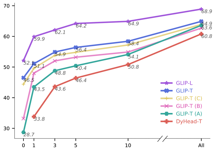
Figure 4: Data efficiency of models. X-axis is the amount of task-specific data, from zero-shot to all data. Y-axis is the average AP across 13 datasets. GLIP exhibits great data efficiency, while each of our proposed approach contributes to the data efficiency.

5.1 Data Efficiency

We vary the amount of task-specific annotated data, from zero-shot (no data provided), to $X$-shot (providing at least $X$ examples per category [24, 66, 62]), to using all data in the training set. We fine-tune the models on the provided data and use the same hyper-parameters for all models. Each dataset comes with pre-specified category names. As GLIP is language-aware, we find it beneficial to re-write some pre-specified names with more descriptive language (see Section 5.2 for a discussion). We compare with the SoTA detector DyHead-T, pre-trained on Objects365. We test with the standard COCO-trained DyHead-T and find it giving similar performance. For simplicity, we report only the former. We also experiment with the scaled cosine similarity approach [61] but find it slightly underperforming the vanilla approach so we report only the latter. Please refer to the appendix for full statistics, including three independent runs for $X$-shot experiments.

Results are shown in Figure 4. We find that unified grounding reformulation, deep fusion, grounding data, and model scale-up all contribute to the improved data efficiency (from the bottom red line (Dyhead-T) up to the upper purple line (GLIP-L)). As a result, GLIP exhibits transformative data efficiency. A zero-shot GLIP-T outperforms 5-shot DyHead-T while a one-shot GLIP-L is competitive with a fully supervised DyHead-T.

We further plot the zero-shot performance of GLIP variants on 5 different datasets in Figure 5. We find that the introduction of grounding data brings significant improvement on certain tasks that test novel concepts, e.g., on Pothole and EgoHands, models without grounding data (A&B) performs terribly, while models with grounding data (C) outperform them with ease.

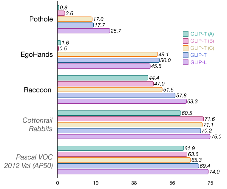
Figure 5: Per dataset zero-shot performance. The first 3 datasets contain novel categories not present in the Objects365 vocabulary while the last 2 datasets’ categories are covered by Objects365 data. Grounding data bring significant benefit to novel categories.

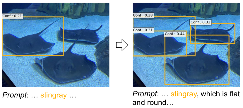
Figure 6: A manual prompt tuning example from the Aquarium dataset in ODinW. Given an expressive prompt (“flat and round”), zero-shot GLIP can detect the novel entity “stingray” better.

5.2 One Model for All Tasks

As neural models become larger, how to reduce deployment cost has drawn an growing research interest. Recent work on language models [52], image classification [72], and object detection [61] has explored adapting a pre-trained model to a new domain but only changing the least amount of parameters. Such a setting is often denoted as linear probing [26], prompt tuning [72], or efficient task adapters [13]. The goal is to have a single model serving various tasks, and each task adds only a few task-specific parameters or no parameters to the pre-trained model. This reduces training and storage cost. In this section, we evaluate models against the metric of deployment efficiency.

Manual prompt tuning. As GLIP performs language-aware localization, i.e., the output of GLIP is heavily conditioned on the language input, we propose an efficient way for GLIP to do task transfer: for any novel categories, the user can use expressive descriptions in the text prompt, adding attributes or language context, to inject domain knowledge and help GLIP transfer. For example, on the left hand side of Figure 6, the model fails to localize all occurrences of the novel entity “stingray”. However, by adding the attributes to the prompt, i.e., “flat and round”, the model successfully localizes all occurrences of stringrays. With this simple prompt change, we improve the AP50 on stingray from 4.6 to 9.7. This resembles the prompt design technique in GPT-3 [3] and is practically appealing, as it requires no annotated data or model re-training. Please refer to the appendix for more details.

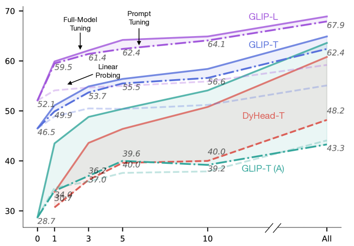
Figure 7: Effectiveness of prompt tuning. Solid lines are full-model tuning performance; dashed lines are prompt/linear probing performance. By only tuning the prompt embeddings, GLIP-T and GLIP-L can achieve performance close to full-model tuning, allowing for efficient deployment.

Prompt tuning. We further consider the setting where we have access to task-specific training data but wish to tune the least amount of parameters for easy deployment. For classical detection models, Wang et al. [61] report the effectiveness of “linear probing” (i.e., train only the box regression and classification head). GLIP can also be “linear probed”, where we only fine-tune the box head and a projection layer between the region and prompt embeddings. Because of the language-aware deep fusion, GLIP supports a more powerful yet still efficient transfer strategy: prompt tuning [52, 31]. For GLIP, as each detection task has only one language prompt (e.g., the prompt for Pothole could be “Detect pothole.” for all images), we first get prompt embeddings $P^{0}$ from the language backbone, then discard the language backbone and only fine-tune $P^{0}$ as the task-specific input (Section 3.2).

We evaluate the models’ performance under three settings (Figure 7): linear probing, prompt tuning (only applicable for GLIP), and full-model tuning. For DyHead-T, prompt tuning is not applicable as the traditional object detection model cannot accept language input; the gap between linear probing and full-model tuning is large. GLIP-T (A) has no language-aware deep fusion; thus prompt tuning and linear tuning achieve similar performance and lag significantly behind full-model tuning. However, for GLIP-T and GLIP-L, prompt tuning almost matches the full-tuning results, without changing any of the grounding model parameters. Interestingly, as the model and data size grow larger, the gap between full-model tuning and prompt tuning becomes smaller (GLIP-L v.s. GLIP-T), echoing the findings in NLP literature [38].

6 Conclusion

GLIP unifies the object detection and phrase grounding tasks to learn an object-level, language-aware, and semantic-rich visual representation. After pre-training, GLIP showed promising results on zero-shot and fine-tuning settings on well-established benchmarks and 13 downstream tasks. We leave a detailed study of how GLIP scales with text-image data size to future work.

Appendix

This appendix is organized as follows.

• In Section A, we provide more visualizations of our model’s grounding predictions on the Conceptual Caption 12M dataset [5].

• In Section B (referred by Section 3.1), we discuss the equivalence between detection and grounding.

• In Section C.1 (referred by Section 4), we introduce the pre-training details of the models we use in Section 4.

• In Section C.2 (referred by Section 4), we introduce the evaluation details of experiments on COCO, LVIS, and Flickr30K.

• In Section C.3 (referred by Section 4), we discuss the difference between the public image-text data (Google Conceptual Captions,SBU) and the image-text data we collected.

• In Section D, we provide a detailed analysis on the computational cost and performance effect of the language-aware deep fusion.

• In Section E.1 (referred by Section 5), we introduce the 13 datasets in Object Detection in the Wild (ODinW).

• In Section E.2 (referred by Section 5), we detail the manual prompt design.

• In Section E.3 (referred by Section 5.1), we give the details for the data efficiency experiments.

• In Section E.4 (referred by Section 5.3), we give the details for the linear probing and prompt tuning experiments.

• In Section E.5, we present per-dataset results for all experiments in Section 5.

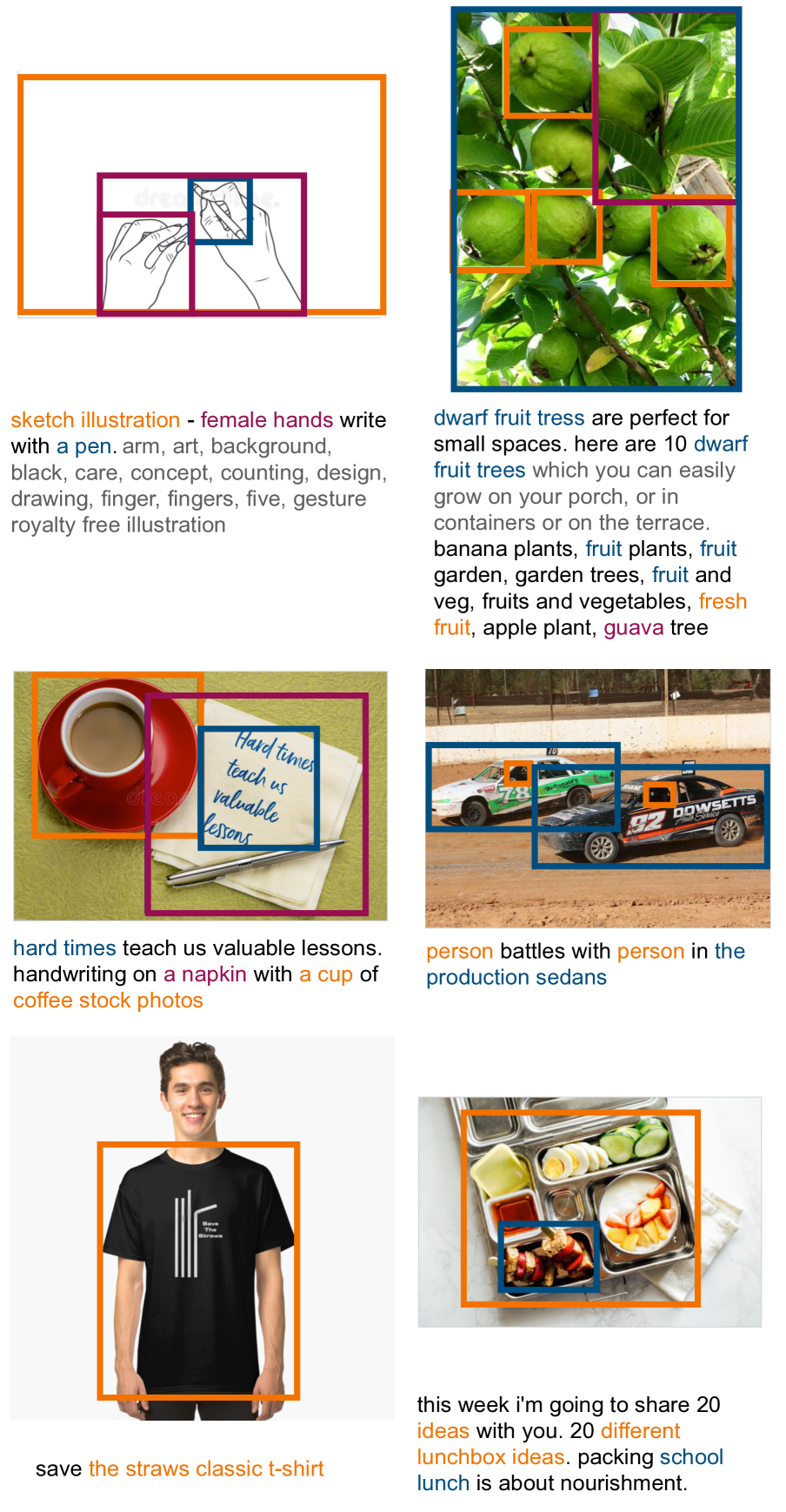
Figure 8: Predictions from the teacher model on 6 examples from Conceptual Captions 12M. Phrases and corresponding boxes are matched with the same colors.

Appendix A Visualization

We provide more visualizations of the predictions from our teacher model. Even given noise image-text pairs, our model is still capable of grounding semantic-rich phrases accurately.

Appendix B Equivalence Discussion between Detection and Grounding

In Section 3.1 of the main paper, we discussed the equivalence between detection and grounding. We corroborate the discussion with empirical experiments.

When all object categories fit into a single prompt.

We first confirm that when all categories fit into one prompt, our grounding formulation is equivalent to classical object detection. We conduct the experiments on COCO [37]. We first choose the SoTA detection model Dynamic Head (DyHead) [10] based on the Swin-Tiny Transformer backbone [39] as the base object detection mode. We then transform this model into a grounding model as described in Section 3.1: we concatenate the 80 class names with “. ” into one prompt and replace DyHead’s classification loss with our grounding loss. We use BERT (base-uncased) [11] to encode the text prompt. When concatenating the class names, we follow a fixed order.

We train the two models with the exact same hyperparameters as in [10]: we train with the standard 2x training configurations [17]. We train with batch size 32 and learning rate $1\times 10^{-4}$ (for the model with grounding reformulation, we use $1\times 10^{-5}$ for the BERT text encoder). We decay the learning rate at 67% and 89% of the total training steps.

The two models achieve the same performance on COCO 2017val: 49.4 AP. Their results are close to the 49.7 reported in the last row of Table 6 of Dai et al. [10] (the small difference is presumably due to the implementation difference). Thus, we conclude that when all categories can fit into a single prompt, grounding and detection tasks are equivalent.

When not all object categories can fit into a single prompt.

The text encoder for the prompt has a limit on the input sentence length. For example, BERT can only encode sentences containing at most 512 tokens. In our implementation, to reduce computational costs, we limit the input length to 256. Thus, for certain datasets with a large vocabulary (e.g., Objects365 [50] has 365 object categories), we cannot fit all category names into one prompt. As a practical solution, we can split the category names into multiple prompts, during both training time and inference time. We find that this incurs minor performance drop. For example, in Table 2 in the main paper, DyHead-T pre-trained on Objects365 achieves 43.6 on COCO zero-shot, while GLIP-T (A) (the grounding reformulated model of DyHead) achieves 42.9 on COCO.

Appendix C Transfer to Established Benchmarks

We introduce the implementation details of the models used in Section 4 and discuss the difference between public image-text data and the data crawled by us.

C.1 Pre-training Details

In Section 4, we introduced GLIP-T (A), GLIP-T (B), GLIP-T (C), GLIP-T, and GLIP-L. We introduce the implementation details in the following. We pre-train models based on Swin-Tiny models with 32 GPUs and a batch size of 64, and models based on Swin-Large with 64 GPUs and a batch size of 64. We use a base learning rate of $1\times 10^{-5}$ for the language backbone and $1\times 10^{-4}$ for all other parameters. The learning rate is stepped down by a factor of 0.1 at the 67% and 89% of the total training steps. We decay the learning rate when the zero-shot performance on COCO saturates. The max input length is 256 tokens for all models.

Table 6: Comparison between public data and data crawled by us.

Pre-Train Data	COCO		LVIS minival				Flickr30K val
	Zero-Shot	Fine-Tune	APr	APc	APf	AP	R@1	R@5	R@10
O365,GoldG,Cap4M	46.3	54.9	20.8	21.4	31.0	26.0	85.7	95.4	96.9
O365,GoldG,CC3M,SBU	46.6	55.2	20.1	21.3	31.1	25.9	85.3	95.7	97.2

Prompt design for detection data.

As noted in Section B, when we pre-train on datasets such as Objects365, we cannot fit all categories into one prompt. During pre-training, we randomly down-sample the categories and keep only the down-sampled categories in the prompt. We randomly shuffle the categories’ order in the prompt.

The down-sampling is done randomly on the fly for each training example and serves as data augmentation. Specifically, for an example, we denote the positive classes that appear in the image as $C_{\text{pos}}$ and the rest negative classes as $C_{\text{neg}}$. We always keep all of $C_{\text{pos}}$. With a probability of $0.5$, we sample from $C_{\text{neg}}$ till we have 85 categories in the prompt; with a probability of $0.5$, we uniformly choose an interger $N$ from $[1,85-|C_{\text{pos}}|]$ and put $N$ categories in the prompt.

Augmentation for image-text data with generated boxes.

When we pre-train the model on image-text data with generated boxes, we find it beneficial to increase the difficulty. We mix a few negative captions (that are from other examples and do not match with the image) with the positive caption (that is matched to the image) to form a longer text input. The model is trained to predict boxes and align them to the correct phrases in the positive caption. The model would need to first identify the positive caption among a few potential captions and then align the box to the correct phrases in the positive caption. This makes the grounding task more challenging and help the model learn a semantic-rich representation during pre-training. This augmentation is also done randomly on the fly. For each training example, with a probability of 0.3, we conduct such augmentation and mix in 19 negative captions; with a probability of 0.3, we mix in a random number (uniformly drawn between 1-19) of negative captions; for the rest of the time, we do not conduct such augmentation.

C.2 Evaluation Details

For fine-tuning on COCO, we use a base learning rate of $1\times 10^{-5}$ for pre-trained models.

For zero-shot evaluation on LVIS, since LVIS has over 1,000 categories and they cannot be fit into one text prompt, we segment them into multiple chunks, fitting 40 categories into one prompt and query the model multiple times with the different prompts. We find that models tend to overfit on LVIS during the course of pre-training so we monitor the performance on minival for all models and report the results with the best checkpoints.

For zero-shot evaluation on Flickr30K, models may also overfit during the course of pre-training so we monitor the performance on the validation set for all models and report the results with the best checkpoints.

C.3 Difference Between Public Data and Web-Crawled Data

For GLIP-T pre-trained with image-text data, as mentioned in Section 4, we train two versions, one with public data (CC3M,SBU) and another with data we crawled (Cap4M). Here we provide a comparison between the two models in Table 6.

The two models differ only slightly, with the Cap4M version better on LVIS while the CC3M+SBU version better on COCO. We conjecture that this is potentially because the public data is more extensively screened and contains more common categories and less rare concepts. Thus it performs slightly better on COCO while lags slightly on LVIS.

Table 7: Computational cost of language-aware deep fusion. For speed, we report FPS, which is the number of images processed per second per GPU (higher is better). For memory consumption, we report the GPU memory used in GB (lower is better). Deep fusion brings less than 1x additional computational cost.

Model	Fusion	Inference (P100)		Train (V100)
		Speed	Memory	Speed	Memory
GLIP-T	✗	4.84 FPS	1.0 GB	2.79 FPS	11.5 GB
	✓	2.52 FPS	2.4 GB	1.62 FPS	16.0 GB
GLIP-L	✗	0.54 FPS	4.8 GB	1.27 FPS	19.7 GB
	✓	0.32 FPS	7.7 GB	0.88 FPS	23.4 GB

Table 8: Language-aware fusion benefits most tasks. We reported the full-model tuning performance for ODinW few-shot results. For models trained with only O365, performance on Flickr30K (grey numbers) is significantly worse because the models are not trained to ground natural language captions.

Deep Fusion	Data	COCO		LVIS minival				Flickr30K val			ODinW
		Zero-Shot	Fine-Tune	APr	APc	APf	AP	R@1	R@5	R@10	0-Shot	1-Shot	3-Shot	5-Shot	10-Shot	Full-Shot
✗	O365	42.9	52.9	14.2	13.9	23.4	18.5	46.4	63.2	66.9	28.7	43.5	48.8	50.4	54.1	63.6
✓	O365	44.9	53.8	13.5	12.8	22.2	17.8	41.4	57.7	61.0	33.2	48.0	52.0	53.2	54.9	62.7
✗	O365,GoldG	41.6	52.9	15.8	23.0	30.8	26.1	82.4	94.7	96.6	35.5	47.2	51.9	53.8	54.3	65.1
✓	O365,GoldG	46.7	55.1	17.7	19.5	31.0	24.9	84.8	94.9	96.3	44.4	49.6	53.8	54.8	57.2	63.9

Appendix D Computation Cost and Performance Analysis of Deep Fusion

In this section, we provide a more detailed ablation on the computational cost and performance effect of the language-aware deep fusion proposed in Section 3.

D.1 Computational Cost

We test the additional computational cost of the language-aware deep fusion for both GLIP-T and GLIP-L. For inference, we test on a P100 GPU with batch size 1. Note that for inference with GLIP without deep fusion, we could cache the language embeddings of the prompts; thus the inference time of GLIP without deep fusion is equivalent to that of DyHead [10].

For training, we test on a standard DGX-2 machine with 16 V100 GPUs (we test under the multi-GPU setting as it mimics the actual training environment): for GLIP-T models, we use 2 images per batch and for GLIP-L models, we use 1 images per batch. As the fusion module invovles multi-head attention over a large number of input elements, we turn on gradient checkpointing for the deep fusion module, which increases training time but reduces GPU memory consumption.

Table 7 shows that the language-aware deep fusion brings less than 1x additional computational cost overall.

D.2 Performance

We provide an analysis on the effect of language-aware deep fusion when different kinds of pre-training data are used. We pre-train four variants of GLIP-T and show the results In Table 8. Deep fusion is beneficial for testing on 1) common categories (i.e., COCO); 2) grounding tasks (i.e., Flickr30K), and 3) low-resource transfer to real-world downstream tasks (i.e., ODinW).

However, on LVIS, the effect of deep fusion seems unclear: when only detection data are used, deep fusion seems to degrades performance (row 1 v.s. row 2); when grounding data are present, deep fusion degrades common category performance but improves rare category performance. Our assumption is that when GLIP is only trained with detection data (e.g., O365), the language model could “overfit” to the categories in O365 and does not generalize to novel categories well (i.e., outputs out-of-distribution text representation). The deep fusion could “amplify” such overfit as the visual representation is conditioned on the language model. Thus, when tested on prompts containing novel categories (e.g., LVIS), deep fusion could degrade performance. When grounding data are used, such overfit could be mitigated.

Appendix E Object Detection in the Wild

In this section, we provide the details and additional results for the experiments in Section 5.

E.1 Dataset Details

We use 13 datasets from Roboflow. Roboflow hosts over 30 datasets and we exclude datasets that are too challenging (e.g., detecting different kinds of chess pieces) or impossible to solve without specific domain knowledge (e.g., understanding sign language).

We provide the details of the 13 datasets we use in Table 9. We include the PASCAL V0C 2012 dataset as a reference dataset, as public baselines have been established on this dataset. For PascalVOC, we follow the convention and report on validation set. For Pistols, there are no official validation or test sets so we split the dataset ourselves.

Table 9: 13 ODinW dataset statistics. We summarize the objects of interest for each dataset and report the image number of each split.

Dataset	Objects of Interest	Train/Val/Test	URL
PascalVOC	Common objects (PascalVOC 2012)	13690/3422/-	https://public.roboflow.com/object-detection/pascal-voc-2012
AerialDrone	Boats, cars, etc. from drone images	52/15/7	https://public.roboflow.com/object-detection/aerial-maritime
Aquarium	Penguins, starfish, etc. in an aquarium	448/127/63	https://public.roboflow.com/object-detection/aquarium
Rabbits	Cottontail rabbits	1980/19/10	https://public.roboflow.com/object-detection/cottontail-rabbits-video-dataset
EgoHands	Hands in ego-centric images	3840/480/480	https://public.roboflow.com/object-detection/hands
Mushrooms	Two kinds of mushrooms	41/5/5	https://public.roboflow.com/object-detection/na-mushrooms
Packages	Delivery packages	19/4/3	https://public.roboflow.com/object-detection/packages-dataset
Raccoon	Raccoon	150/29/17	https://public.roboflow.com/object-detection/raccoon
Shellfish	Shrimp, lobster, and crab	406/116/58	https://public.roboflow.com/object-detection/shellfish-openimages
Vehicles	Car, bus, motorcycle, truck, and ambulance	878/250/126	https://public.roboflow.com/object-detection/vehicles-openimages
Pistols	Pistol	2377/297/297	https://public.roboflow.com/object-detection/pistols/1
Pothole	Potholes on the road	465/133/67	https://public.roboflow.com/object-detection/pothole
Thermal	Dogs and people in thermal images	142/41/20	https://public.roboflow.com/object-detection/thermal-dogs-and-people

E.2 Manual Prompt Tuning

As discussed in Section 5, we find it beneficial to manually design some prompts to provide language guidance. We provide the prompts we use in Table 10. We design the prompts for 6 datasets. Since some prompts are sentences, we only apply these prompts for models trained with grounding data (GLIP-T (C), GLIP-T, and GLIP-L). For GLIP-T (A) and GLIP-T (B), we find it beneficial to use prompts for the Rabbits and Mushrooms datasets, as the prompts there are just single word or short phrases. Overall, using prompts improves AP without any model re-training (e.g., the AP improves from 22.1 to 50.0 for EgoHands).

Table 10: Manually designed prompts for 6 datasets. Words in italic are the objects of interest. The prompts either provide attributes, specify the category name in more common words, or provide language contexts. They can improve AP (CLIP-T) without any annotation or model re-training. Specifically for Pothole, although the changed prompt does not improve the AP of CLIP-T, we find it effective for CLIP-T (C) so we still apply the prompt.

Dataset	Original Prompt	AP	Manually Designed Prompts	AP
Aquarium	penguin	17.7	penguin, which is black and white	18.4
	puffin		puffin with orange beaks
	stingray		stingray which is flat and round
Rabbits	Cottontail-Rabbits	68.0	rabbit	70.2
EgoHands	hand	22.1	hand of a person	50.0
Mushrooms	Cow. Chanterelle	13.6	flat mushroom. yellow mushroom	73.8
Packages	package	50.0	there is a package on the porch	72.3
Pothole	pothole	17.8	there are some holes on the road	17.7

Table 11: Zero-shot and full fine-tuning performance. GLIP models exhibit superior data efficiency.

Model	Zero Shot	Full Tuning
		1	3	5	10	All
DyHead-T COCO	-	31.9$\pm$4.1	44.2$\pm$0.4	44.7$\pm$2.1	50.1$\pm$2.0	63.2
DyHead-T O365	-	33.8$\pm$4.3	43.6$\pm$1.2	46.4$\pm$1.4	50.8$\pm$1.6	60.8
GLIP-T (A)	28.7	43.5$\pm$1.5	48.8$\pm$0.4	50.4$\pm$0.7	54.1$\pm$0.5	63.6
GLIP-T (B)	33.2	48.0$\pm$0.8	52.0$\pm$0.4	53.2$\pm$0.9	54.9$\pm$0.7	62.7
GLIP-T (C)	44.4	49.6$\pm$0.3	53.8$\pm$0.2	54.8$\pm$1.0	57.2$\pm$1.1	63.9
GLIP-T	46.5	51.1$\pm$0.1	54.9$\pm$0.3	56.4$\pm$0.5	58.4$\pm$0.2	64.9
GLIP-L	52.1	59.9$\pm$1.7	62.1$\pm$0.8	64.2$\pm$0.4	64.9$\pm$0.9	68.9

E.3 Data Efficiency

We provide details for the experiments in Section 5.1. We train with batch size 4, learning rate $1\times 10^{-4}$ (for the model with grounding reformulation, we use $1\times 10^{-5}$ for the BERT text encoder), and weight decay of 0.05. We do not find that increasing batch size improves performance significantly. For computational reasons, we use a batch size of 4. Following convention, we freeze the bottom 2 layers of the backbone during fine-tuning. We monitor the performance on validation and decay the learning rate by 0.1 when the validation performance plateaus. In $X$-shot settings, we randomly sample the dataset such that there are at least $X$ examples per category [24]. We change the random seeds (and thus change the sampled data) and conduct 3 independent runs for each $X$-shot experiment. We provide two DyHead-T variants as baselines, one trained on COCO and one trained on Objects365. We report the full zero-shot results in Table 14 and few-shot results in Table 11.

Table 12: Linear probing performance.

Model	Linear Probing
	1	3	5	10	All
DyHead-T COCO	22.7$\pm$1.1	32.7$\pm$1.4	30.5$\pm$2.9	34.1$\pm$1.4	43.1
DyHead-T COCO-Cosine	21.8$\pm$4.4	30.6$\pm$2.2	33.3$\pm$1.2	35.5$\pm$1.2	43.5
DyHead-T O365	30.7$\pm$3.3	36.2$\pm$3.3	39.6$\pm$0.4	40.0$\pm$2.7	48.2
DyHead-T O365-Cosine	25.2$\pm$2.6	37.6$\pm$0.5	38.9$\pm$0.7	41.5$\pm$0.5	49.4
GLIP-T (A)	34.6$\pm$0.7	35.9$\pm$0.2	37.6$\pm$0.1	37.9$\pm$0.2	44.1
GLIP-T (B)	40.9$\pm$0.3	42.8$\pm$0.4	44.0$\pm$0.2	44.4$\pm$0.3	51.8
GLIP-T (C)	43.9$\pm$0.1	45.4$\pm$0.1	45.9$\pm$0.2	46.7$\pm$0.3	52.7
GLIP-T	48.9$\pm$0.2	50.5$\pm$0.1	50.4$\pm$0.3	51.2$\pm$0.2	55.1
GLIP-L	54.1$\pm$0.3	54.7$\pm$0.2	55.0$\pm$0.0	55.9$\pm$0.4	59.2

Table 13: Prompt tuning performance.

Model	Prompt Probing
	1	3	5	10	All
GLIP-T (A)	34.0$\pm$0.1	37.0$\pm$0.6	40.0$\pm$0.4	39.2$\pm$1.0	43.3
GLIP-T (B)	46.4$\pm$0.5	49.0$\pm$0.9	50.6$\pm$0.5	52.7$\pm$0.1	58.5
GLIP-T (C)	50.6$\pm$0.5	52.9$\pm$0.5	53.9$\pm$0.7	55.8$\pm$1.1	62.8
GLIP-T	49.9$\pm$0.7	53.7$\pm$1.6	55.5$\pm$0.6	56.6$\pm$0.3	62.4
GLIP-L	59.5$\pm$0.4	61.4$\pm$0.4	62.4$\pm$0.6	64.1$\pm$0.6	67.9

E.4 One Model for All Tasks

In Section 5.2, we conduct experiments with respect to deployment efficiency: tuning the least amount of parameters for the best performance. For all models, we experiment with the linear probing setting; for GLIP models, we also experiment with the prompt tuning setting. For linear probing, we try both the vanilla approach (simply tune the classification and localization head) and the cosine scale approach [61]. Below we provide the implementation details.

For the vanilla linear probing, we train with a learning rate of $1\times 10^{-4}$, batch size of 4, and weight decay of 0.05. For linear probing with the cosine scale, we use a scale of $20.0$ per suggestions of Wang et al. [61], learning rate of $0.01$, batch size of 4, and weight decay of 0.05. For prompt tuning, we train with a learning rate of $0.05$, batch size of 4, and weight decay of 0.25. We have conducted preliminary searches for the hyper-parameters.

Results are present in Table 12 (linear probing) and Table 13 (prompt tuning). Comparing them with full-tuning results (Table 11), we see prompt tuning performance of GLIP is competitive, showing the deployment efficiency. Contrary to Wang et al. [61] who report that linear probing can deliver competitive performance for classical detection models, we find that linear probing does not work well compared to full tuning. We find that the reason could be the transfer datasets (ODinW) in our case contain a lot of novel tasks and domains, while experiments in Wang et al. focus on transferring to common domains (e.g., PascalVOC and COCO). In Table 15, we report the per-dataset performance. We find that for some common tasks or domains (e.g., PascalVOC and Vehicles), linear probing of DyHead COCO performs competitively with full fine-tuning but the gap is large for some other tasks of a novel domain (e.g., AerialDrone).

E.5 All Results

We report the per-dataset performance under 0,1,3,5,10-shot and full data as well as linear probing, prompt tuning, and full-model tuning in Table 14, Table 15, and Table 16 (on the next pages).

Table 14: Zero-shot performance on 13 ODinW datasets.

Model	PascalVOC	AerialDrone	Aquarium	Rabbits	EgoHands	Mushrooms	Packages	Raccoon	Shellfish	Vehicles	Pistols	Pothole	Thermal	Avg
GLIP-T (A)	47.7	9.8	16.8	60.5	1.6	13.7	48.5	44.4	20.4	52.4	25.3	0.8	32.3	28.8
GLIP-T (B)	50.6	4.9	19.4	71.6	0.5	21.8	29.7	47.0	21.4	56.0	47.4	3.6	57.1	33.2
GLIP-T (C)	51.6	8.1	22.6	71.1	49.1	69.4	65.6	51.5	29.3	49.9	42.7	17.0	49.2	44.4
GLIP-T	56.2	12.5	18.4	70.2	50.0	73.8	72.3	57.8	26.3	56.0	49.6	17.7	44.1	46.5
GLIP-L	61.7	7.1	26.9	75.0	45.5	49.0	62.8	63.3	68.9	57.3	68.6	25.7	66.0	52.1

Table 15: Per-dataset performance of DyHead, GLIP-T, and GLIP-L. For PascalVOC, we report the mAP (IoU=0.50:0.95) using the COCO evaluation script, to be consistent with other 12 datasets. “Linear” denotes linear probing. “Prompt” denotes prompt tuning. “Full” denotes full-model tuning.

Model

Shot

Tune

PascalVOC

AerialDrone

Aquarium

Rabbits

EgoHands

Mushrooms

Packages

Raccoon

Shellfish

Vehicles

Pistols

Pothole

Thermal

Avg

DyHead COCO

1

Linear

48.2$\pm$2.4

2.7$\pm$2.0

8.5$\pm$1.5

57.8$\pm$3.2

9.7$\pm$3.4

30.2$\pm$18.3

13.2$\pm$9.4

30.2$\pm$4.0

9.9$\pm$4.0

42.5$\pm$4.1

5.7$\pm$7.1

2.6$\pm$2.0

34.2$\pm$19.7

22.7$\pm$0.9

DyHead COCO

3

Linear

55.6$\pm$0.6

2.7$\pm$3.0

12.3$\pm$0.5

57.4$\pm$3.1

15.4$\pm$2.1

57.1$\pm$1.6

30.6$\pm$16.9

55.4$\pm$1.6

14.8$\pm$1.4

51.0$\pm$3.9

22.8$\pm$3.1

8.7$\pm$1.0

41.5$\pm$11.1

32.7$\pm$1.1

DyHead COCO

5

Linear

56.4$\pm$0.2

2.7$\pm$2.4

14.1$\pm$0.9

54.7$\pm$4.9

8.8$\pm$6.6

47.1$\pm$12.6

24.6$\pm$22.9

51.6$\pm$2.9

17.0$\pm$0.6

46.6$\pm$3.0

20.3$\pm$13.9

7.8$\pm$2.1

44.3$\pm$4.2

30.5$\pm$2.4

DyHead COCO

10

Linear

57.4$\pm$0.3

7.4$\pm$0.7

16.0$\pm$2.2

59.8$\pm$0.8

18.6$\pm$0.3

55.0$\pm$0.8

30.8$\pm$17.1

53.0$\pm$4.0

16.7$\pm$0.7

50.7$\pm$0.9

27.8$\pm$1.9

3.1$\pm$4.3

47.5$\pm$3.1

34.1$\pm$1.2

DyHead COCO

All

Linear

61.3

10.3

21.6

61.4

39.0

55.4

54.4

57.3

23.1

60.7

47.9

14.9

53.5

43.1

DyHead COCO

1

Full

31.7$\pm$3.1

14.3$\pm$2.4

13.1$\pm$2.0

63.6$\pm$1.4

40.9$\pm$7.0

67.0$\pm$3.6

34.6$\pm$12.1

45.9$\pm$3.8

10.8$\pm$5.0

34.0$\pm$3.3

12.0$\pm$10.4

6.1$\pm$1.3

40.9$\pm$7.4

31.9$\pm$3.3

DyHead COCO

3

Full

44.1$\pm$0.7

19.2$\pm$3.0

22.6$\pm$1.3

64.8$\pm$1.7

54.4$\pm$2.5

78.9$\pm$1.3

61.6$\pm$10.3

50.0$\pm$2.1

20.8$\pm$3.5

44.9$\pm$1.9

34.4$\pm$11.1

20.6$\pm$2.4

57.9$\pm$2.3

44.2$\pm$0.3

DyHead COCO

5

Full

44.9$\pm$1.5

22.2$\pm$3.0

31.7$\pm$1.0

65.2$\pm$1.5

55.6$\pm$3.7

78.7$\pm$3.9

50.1$\pm$13.7

48.7$\pm$4.8

22.8$\pm$3.3

52.0$\pm$1.2

39.8$\pm$6.7

20.9$\pm$1.5

48.0$\pm$2.8

44.7$\pm$1.7

DyHead COCO

10

Full

48.4$\pm$1.2

27.5$\pm$1.4

39.3$\pm$2.7

62.1$\pm$5.9

61.6$\pm$1.4

81.7$\pm$3.4

58.8$\pm$9.0

52.9$\pm$3.2

30.1$\pm$3.2

54.1$\pm$3.3

44.8$\pm$4.9

26.7$\pm$2.4

63.4$\pm$2.8

50.1$\pm$1.6

DyHead COCO

All

Full

60.1

27.6

53.1

76.5

79.4

86.1

69.3

55.2

44.0

61.5

70.6

56.6

81.0

63.2

DyHead O365

1

Linear

45.2$\pm$3.0

10.8$\pm$3.6

13.8$\pm$0.7

61.4$\pm$0.7

8.9$\pm$6.3

52.6$\pm$8.7

58.7$\pm$3.7

44.0$\pm$10.4

14.9$\pm$2.9

40.0$\pm$0.4

6.9$\pm$5.0

1.7$\pm$1.2

39.8$\pm$7.2

30.7$\pm$2.7

DyHead O365

3

Linear

54.6$\pm$0.4

12.4$\pm$3.0

22.3$\pm$1.5

64.0$\pm$2.4

10.5$\pm$6.8

53.6$\pm$10.6

49.1$\pm$16.3

60.5$\pm$1.6

20.6$\pm$2.2

51.3$\pm$2.3

25.5$\pm$0.9

8.2$\pm$1.1

38.9$\pm$12.6

36.3$\pm$2.7

DyHead O365

5

Linear

56.1$\pm$0.4

13.6$\pm$1.8

24.8$\pm$1.1

63.1$\pm$5.5

15.3$\pm$1.6

55.2$\pm$10.3

70.2$\pm$2.8

60.1$\pm$2.4

23.0$\pm$1.4

53.5$\pm$0.9

26.1$\pm$2.1

6.8$\pm$2.3

46.9$\pm$3.5

39.6$\pm$0.4

DyHead O365

10

Linear

57.5$\pm$0.3

8.2$\pm$3.0

28.2$\pm$0.8

65.4$\pm$3.2

17.5$\pm$0.6

68.0$\pm$0.8

49.8$\pm$17.3

60.3$\pm$2.1

22.9$\pm$1.0

56.4$\pm$0.8

28.0$\pm$2.2

7.6$\pm$0.9

50.3$\pm$0.5

40.0$\pm$2.2

DyHead O365

All

Linear

63.0

18.9

33.7

69.2

36.3

70.9

52.4

66.7

26.6

60.6

48.2

16.1

64.6

48.2

DyHead O365

1

Full

25.8$\pm$3.0

16.5$\pm$1.8

15.9$\pm$2.7

55.7$\pm$6.0

44.0$\pm$3.6

66.9$\pm$3.9

54.2$\pm$5.7

50.7$\pm$7.7

14.1$\pm$3.6

33.0$\pm$11.0

11.0$\pm$6.5

8.2$\pm$4.1

43.2$\pm$10.0

33.8$\pm$3.5

DyHead O365

3

Full

40.4$\pm$1.0

20.5$\pm$4.0

26.5$\pm$1.3

57.9$\pm$2.0

53.9$\pm$2.5

76.5$\pm$2.3

62.6$\pm$13.3

52.5$\pm$5.0

22.4$\pm$1.7

47.4$\pm$2.0

30.1$\pm$6.9

19.7$\pm$1.5

57.0$\pm$2.3

43.6$\pm$1.0

DyHead O365

5

Full

43.5$\pm$1.0

25.3$\pm$1.8

35.8$\pm$0.5

63.0$\pm$1.0

56.2$\pm$3.9

76.8$\pm$5.9

62.5$\pm$8.7

46.6$\pm$3.1

28.8$\pm$2.2

51.2$\pm$2.2

38.7$\pm$4.1

21.0$\pm$1.4

53.4$\pm$5.2

46.4$\pm$1.1

DyHead O365

10

Full

46.6$\pm$0.3

29.0$\pm$2.8

41.7$\pm$1.0

65.2$\pm$2.5

62.5$\pm$0.8

85.4$\pm$2.2

67.9$\pm$4.5

47.9$\pm$2.2

28.6$\pm$5.0

53.8$\pm$1.0

39.2$\pm$4.9

27.9$\pm$2.3

64.1$\pm$2.6

50.8$\pm$1.3

DyHead O365

All

Full

53.3

28.4

49.5

73.5

77.9

84.0

69.2

56.2

43.6

59.2

68.9

53.7

73.7

60.8

GLIP-T

1

Linear

57.1$\pm$0.0

15.0$\pm$0.3

21.2$\pm$0.3

68.3$\pm$1.6

59.5$\pm$0.1

72.7$\pm$0.3

72.3$\pm$0.0

65.2$\pm$0.2

26.5$\pm$0.1

57.6$\pm$0.1

54.1$\pm$0.4

18.2$\pm$0.1

47.3$\pm$0.2

48.9$\pm$0.1

GLIP-T

3

Linear

58.9$\pm$0.1

15.3$\pm$0.1

26.0$\pm$0.3

70.1$\pm$0.5

61.6$\pm$0.4

74.7$\pm$0.1

72.3$\pm$0.0

64.6$\pm$0.2

25.9$\pm$0.0

60.1$\pm$0.1

51.0$\pm$0.2

20.9$\pm$0.1

55.5$\pm$0.2

50.5$\pm$0.1

GLIP-T

5

Linear

59.0$\pm$0.1

15.5$\pm$0.4

27.6$\pm$0.9

69.7$\pm$0.8

61.8$\pm$0.1

75.1$\pm$0.4

72.3$\pm$0.0

62.8$\pm$0.5

25.4$\pm$0.4

62.5$\pm$0.6

51.4$\pm$0.3

19.6$\pm$0.6

52.7$\pm$1.2

50.4$\pm$0.2

GLIP-T

10

Linear

60.1$\pm$0.1

14.1$\pm$0.1

29.6$\pm$0.8

69.5$\pm$0.3

62.4$\pm$0.2

76.8$\pm$0.1

72.3$\pm$0.0

61.1$\pm$0.3

25.8$\pm$0.2

63.4$\pm$0.6

51.0$\pm$0.1

23.3$\pm$0.3

55.8$\pm$1.3

51.2$\pm$0.1

GLIP-T

All

Linear

65.5

14.1

36.5

68.2

67.2

76.6

70.2

63.8

29.1

65.5

63.5

29.9

66.5

55.1

GLIP-T

1

Prompt

54.4$\pm$0.9

15.2$\pm$1.4

32.5$\pm$1.0

68.0$\pm$3.2

60.0$\pm$0.7

75.8$\pm$1.2

72.3$\pm$0.0

54.5$\pm$3.9

24.1$\pm$3.0

59.2$\pm$0.9

57.4$\pm$0.6

18.9$\pm$1.8

56.9$\pm$2.7

49.9$\pm$0.6

GLIP-T

3

Prompt

56.8$\pm$0.8

18.9$\pm$3.6

37.6$\pm$1.6

72.4$\pm$0.5

62.8$\pm$1.3

85.4$\pm$2.8

64.5$\pm$4.6

69.1$\pm$1.8

22.0$\pm$0.9

62.7$\pm$1.1

56.1$\pm$0.6

25.9$\pm$0.7

63.8$\pm$4.8

53.7$\pm$1.3

GLIP-T

5

Prompt

58.5$\pm$0.5

18.2$\pm$0.1

41.0$\pm$1.2

71.8$\pm$2.4

65.7$\pm$0.7

87.5$\pm$2.2

72.3$\pm$0.0

60.6$\pm$2.2

31.4$\pm$4.2

61.0$\pm$1.8

54.4$\pm$0.6

32.6$\pm$1.4

66.3$\pm$2.8

55.5$\pm$0.5

GLIP-T

10

Prompt

59.7$\pm$0.7

19.8$\pm$1.6

44.8$\pm$0.9

72.1$\pm$2.0

65.9$\pm$0.6

87.4$\pm$1.1

72.3$\pm$0.0

57.5$\pm$1.2

30.0$\pm$1.4

62.1$\pm$1.4

57.8$\pm$0.9

33.5$\pm$0.1

73.1$\pm$1.4

56.6$\pm$0.2

GLIP-T

All

Prompt

66.4

27.6

50.9

70.6

73.3

88.1

67.7

64.0

40.3

65.4

68.3

50.7

78.5

62.4

GLIP-T

1

Full

54.8$\pm$2.0

18.4$\pm$1.0

33.8$\pm$1.1

70.1$\pm$2.9

64.2$\pm$1.8

83.7$\pm$3.0

70.8$\pm$2.1

56.2$\pm$1.8

22.9$\pm$0.2

56.6$\pm$0.5

59.9$\pm$0.4

18.9$\pm$1.3

54.5$\pm$2.7

51.1$\pm$0.1

GLIP-T

3

Full

58.1$\pm$0.5

22.9$\pm$1.3

40.8$\pm$0.9

65.7$\pm$1.6

66.0$\pm$0.2

84.7$\pm$0.5

65.7$\pm$2.8

62.6$\pm$1.4

27.2$\pm$2.7

61.9$\pm$1.8

60.7$\pm$0.2

27.1$\pm$1.2

70.4$\pm$2.5

54.9$\pm$0.2

GLIP-T

5

Full

59.5$\pm$0.4

23.8$\pm$0.9

43.6$\pm$1.4

68.7$\pm$1.3

66.1$\pm$0.6

85.4$\pm$0.4

72.3$\pm$0.0

62.1$\pm$2.0

27.3$\pm$1.2

61.0$\pm$1.8

62.7$\pm$1.6

34.5$\pm$0.5

66.6$\pm$2.3

56.4$\pm$0.4

GLIP-T

10

Full

59.1$\pm$1.3

26.3$\pm$1.1

46.3$\pm$1.6

67.3$\pm$1.5

67.1$\pm$0.7

87.8$\pm$0.5

72.3$\pm$0.0

57.7$\pm$1.7

34.6$\pm$1.7

65.4$\pm$1.4

61.6$\pm$1.0

39.3$\pm$1.0

74.7$\pm$2.3

58.4$\pm$0.2

GLIP-T

All

Full

62.3

31.2

52.5

70.8

78.7

88.1

75.6

61.4

51.4

65.3

71.2

58.7

76.7

64.9

GLIP-L

1

Linear

63.7$\pm$0.1

7.6$\pm$0.3

28.1$\pm$0.2

74.6$\pm$0.0

60.3$\pm$0.0

41.3$\pm$3.1

70.2$\pm$1.3

67.0$\pm$1.0

71.0$\pm$0.0

60.5$\pm$0.3

67.9$\pm$0.1

24.8$\pm$0.0

66.1$\pm$0.0

54.1$\pm$0.3

GLIP-L

3

Linear

64.8$\pm$0.1

8.5$\pm$0.1

33.7$\pm$0.2

74.3$\pm$0.2

64.1$\pm$0.2

37.0$\pm$0.2

69.3$\pm$0.0

66.6$\pm$1.9

71.2$\pm$0.3

63.2$\pm$0.3

68.0$\pm$0.1

24.8$\pm$0.0

65.9$\pm$0.4

54.7$\pm$0.2

GLIP-L

5

Linear

65.0$\pm$0.1

8.8$\pm$0.1

33.4$\pm$0.3

74.1$\pm$0.1

63.8$\pm$0.0

37.2$\pm$0.0

69.3$\pm$0.0

69.2$\pm$0.6

71.5$\pm$0.1

64.2$\pm$0.3

68.0$\pm$0.1

25.3$\pm$0.2

65.2$\pm$0.5

55.0$\pm$0.0

GLIP-L

10

Linear

65.2$\pm$0.3

11.5$\pm$2.3

35.1$\pm$0.4

74.0$\pm$0.0

64.7$\pm$0.0

38.0$\pm$1.0

71.7$\pm$1.7

66.7$\pm$0.3

72.5$\pm$0.3

65.6$\pm$1.1

67.9$\pm$0.0

25.8$\pm$0.2

67.2$\pm$0.3

55.8$\pm$0.4

GLIP-L

All

Linear

70.9

9.6

42.3

75.3

70.5

39.4

69.3

71.6

73.9

69.7

72.1

33.2

72.3

59.2

GLIP-L

1

Prompt

62.8$\pm$0.4

18.0$\pm$1.8

37.4$\pm$0.3

71.9$\pm$2.4

68.9$\pm$0.1

81.8$\pm$3.4

65.0$\pm$2.8

63.9$\pm$0.4

70.2$\pm$1.2

67.0$\pm$0.4

69.3$\pm$0.1

27.6$\pm$0.4

69.8$\pm$0.6

59.5$\pm$0.4

GLIP-L

3

Prompt

65.0$\pm$0.5

21.4$\pm$1.0

43.6$\pm$1.1

72.9$\pm$0.7

70.4$\pm$0.1

91.4$\pm$0.7

57.7$\pm$3.7

70.7$\pm$1.1

69.7$\pm$0.9

62.6$\pm$0.8

67.7$\pm$0.4

36.2$\pm$1.1

68.8$\pm$1.5

61.4$\pm$0.3

GLIP-L

5

Prompt

65.6$\pm$0.3

19.9$\pm$1.6

47.7$\pm$0.7

73.7$\pm$0.7

70.6$\pm$0.3

86.8$\pm$0.5

64.6$\pm$0.7

69.4$\pm$3.3

68.0$\pm$1.3

67.8$\pm$1.5

68.3$\pm$0.3

36.6$\pm$1.6

71.9$\pm$0.6

62.4$\pm$0.5

GLIP-L

10

Prompt

65.9$\pm$0.2

23.4$\pm$2.6

50.3$\pm$0.7

73.6$\pm$0.7

71.8$\pm$0.3

86.5$\pm$0.3

70.5$\pm$1.1

69.0$\pm$0.5

69.4$\pm$2.4

70.8$\pm$1.2

68.8$\pm$0.6

39.3$\pm$0.9

74.9$\pm$2.1

64.2$\pm$0.4

GLIP-L

All

Prompt

72.9

23.0

51.8

72.0

75.8

88.1

75.2

69.5

73.6

72.1

73.7

53.5

81.4

67.9$\pm$0.0

GLIP-L

1

Full

64.8$\pm$0.6

18.7$\pm$0.6

39.5$\pm$1.2

70.0$\pm$1.5

70.5$\pm$0.2

69.8$\pm$18.0

70.6$\pm$4.0

68.4$\pm$1.2

71.0$\pm$1.3

65.4$\pm$1.1

68.1$\pm$0.2

28.9$\pm$2.9

72.9$\pm$4.7

59.9$\pm$1.4

GLIP-L

3

Full

65.6$\pm$0.6

22.3$\pm$1.1

45.2$\pm$0.4

72.3$\pm$1.4

70.4$\pm$0.4

81.6$\pm$13.3

71.8$\pm$0.3

65.3$\pm$1.6

67.6$\pm$1.0

66.7$\pm$0.9

68.1$\pm$0.3

37.0$\pm$1.9

73.1$\pm$3.3

62.1$\pm$0.7

GLIP-L

5

Full

66.6$\pm$0.4

26.4$\pm$2.5

49.5$\pm$1.1

70.7$\pm$0.2

71.9$\pm$0.2

88.1$\pm$0.0

71.1$\pm$0.6

68.8$\pm$1.2

68.5$\pm$1.7

70.0$\pm$0.9

68.3$\pm$0.5

39.9$\pm$1.4

75.2$\pm$2.7

64.2$\pm$0.3

GLIP-L

10

Full

66.4$\pm$0.7

32.0$\pm$1.4

52.3$\pm$1.1

70.6$\pm$0.7

72.4$\pm$0.3

88.1$\pm$0.0

67.1$\pm$3.6

64.7$\pm$3.1

69.4$\pm$1.4

71.5$\pm$0.8

68.4$\pm$0.7

44.3$\pm$0.6

76.3$\pm$1.1

64.9$\pm$0.7

GLIP-L

All

Full

69.6

32.6

56.6

76.4

79.4

88.1

67.1

69.4

65.8

71.6

75.7

60.3

83.1

68.9

Table 16: Per-dataset performance of GLIP-T (A, B, and C). For PascalVOC, we report the mAP (IoU=0.50:0.95) using the COCO evaluation script, to be consistent with other 12 datasets. “Linear” denotes linear probing. “Prompt” denotes prompt tuning. “Full” denotes full-model tuning.

Model

Shot

Tune

PascalVOC

AerialDrone

Aquarium

Rabbits

EgoHands

Mushrooms

Packages

Raccoon

Shellfish

Vehicles

Pistols

Pothole

Thermal

Avg

GLIP-T (A)

1

Linear

52.9$\pm$0.1

13.2$\pm$0.3

21.3$\pm$3.2

65.0$\pm$2.0

23.1$\pm$0.3

11.4$\pm$0.1

57.3$\pm$4.6

53.5$\pm$0.7

16.8$\pm$0.0

54.1$\pm$0.1

34.5$\pm$0.2

5.8$\pm$0.1

40.8$\pm$0.4

34.6$\pm$0.6

GLIP-T (A)

3

Linear

54.6$\pm$0.2

13.4$\pm$0.1

28.3$\pm$0.1

65.4$\pm$1.0

26.0$\pm$0.3

11.4$\pm$0.0

50.8$\pm$0.7

58.8$\pm$0.3

15.8$\pm$0.7

56.1$\pm$1.0

34.4$\pm$0.9

6.5$\pm$0.0

45.8$\pm$0.3

35.9$\pm$0.2

GLIP-T (A)

5

Linear

55.3$\pm$0.1

14.0$\pm$0.3

28.5$\pm$0.1

65.2$\pm$1.3

28.4$\pm$0.2

11.7$\pm$0.0

63.9$\pm$0.0

59.2$\pm$0.8

16.9$\pm$0.2

56.6$\pm$0.2

36.9$\pm$0.5

9.3$\pm$0.0

43.2$\pm$0.3

37.6$\pm$0.1

GLIP-T (A)

10

Linear

56.8$\pm$0.2

14.3$\pm$0.2

29.0$\pm$0.1

67.0$\pm$0.1

29.2$\pm$0.1

11.6$\pm$0.1

64.5$\pm$0.3

59.7$\pm$0.7

16.6$\pm$0.7

56.9$\pm$0.0

33.2$\pm$1.5

7.4$\pm$0.1

46.2$\pm$0.8

37.9$\pm$0.2

GLIP-T (A)

All

Linear

62.0

15.1

32.2

66.1

40.9

12.1

66.9

60.5

22.5

62.4

49.8

17.1

65.7

44.1$\pm$0.0

GLIP-T (A)

1

Prompt

52.1$\pm$0.5

11.4$\pm$0.2

23.7$\pm$0.6

66.6$\pm$0.2

21.0$\pm$0.2

8.6$\pm$0.6

46.7$\pm$0.1

53.2$\pm$0.2

17.1$\pm$0.7

58.8$\pm$0.2

37.9$\pm$0.3

6.0$\pm$0.2

38.3$\pm$0.4

34.0$\pm$0.1

GLIP-T (A)

3

Prompt

54.9$\pm$0.1

13.4$\pm$2.5

25.9$\pm$0.2

65.9$\pm$0.5

22.7$\pm$0.1

33.6$\pm$1.4

46.6$\pm$0.0

53.7$\pm$0.4

18.5$\pm$0.8

58.2$\pm$0.6

38.1$\pm$0.5

6.2$\pm$0.1

42.4$\pm$0.2

36.9$\pm$0.5

GLIP-T (A)

5

Prompt

55.6$\pm$0.2

13.6$\pm$0.4

26.1$\pm$0.4

65.7$\pm$1.5

24.5$\pm$0.4

56.9$\pm$2.6

60.5$\pm$0.6

55.2$\pm$0.2

19.0$\pm$1.5

57.0$\pm$0.8

36.4$\pm$1.4

6.3$\pm$0.1

43.2$\pm$0.1

40.0$\pm$0.3

GLIP-T (A)

10

Prompt

56.6$\pm$0.1

15.8$\pm$0.8

26.2$\pm$0.1

68.0$\pm$0.6

24.4$\pm$0.1

41.2$\pm$12.5

60.3$\pm$0.9

55.9$\pm$0.4

19.6$\pm$1.6

57.5$\pm$1.0

36.1$\pm$0.3

6.0$\pm$0.1

42.4$\pm$1.2

39.2$\pm$0.9

GLIP-T (A)

All

Prompt

58.8

16.4

28.7

69.5

28.8

56.9

60.9

56.3

20.5

60.7

43.3

10.4

51.2

43.3

GLIP-T (A)

1

Full

44.8$\pm$0.7

16.9$\pm$1.2

28.0$\pm$1.0

64.6$\pm$1.6

54.1$\pm$1.5

64.1$\pm$12.0

55.8$\pm$0.6

55.6$\pm$1.8

21.6$\pm$0.9

53.4$\pm$1.3

43.8$\pm$0.9

10.9$\pm$1.2

52.3$\pm$4.7

43.5$\pm$1.2

GLIP-T (A)

3

Full

49.5$\pm$0.6

23.3$\pm$1.4

36.7$\pm$1.2

62.5$\pm$1.6

59.9$\pm$1.1

84.1$\pm$1.3

60.2$\pm$1.1

45.0$\pm$2.6

26.5$\pm$1.9

54.4$\pm$0.7

44.6$\pm$3.7

23.6$\pm$0.7

63.5$\pm$2.7

48.8$\pm$0.3

GLIP-T (A)

5

Full

50.8$\pm$0.5

25.3$\pm$0.7

41.2$\pm$0.8

62.4$\pm$0.9

60.4$\pm$0.9

86.4$\pm$2.3

59.2$\pm$8.5

44.7$\pm$2.5

28.2$\pm$0.7

55.6$\pm$2.0

51.7$\pm$0.8

27.0$\pm$0.8

62.1$\pm$6.0

50.4$\pm$0.6

GLIP-T (A)

10

Full

51.7$\pm$0.3

29.9$\pm$2.4

44.3$\pm$0.8

67.8$\pm$2.7

64.1$\pm$0.3

87.9$\pm$0.3

71.3$\pm$2.0

47.0$\pm$4.2

28.8$\pm$2.0

56.9$\pm$0.9

52.3$\pm$0.4

29.1$\pm$2.9

72.7$\pm$2.2

54.1$\pm$0.4

GLIP-T (A)

All

Full

55.1

35.3

50.9

78.0

78.0

86.3

75.2

54.8

44.1

61.4

69.3

57.3

80.6

63.6

GLIP-T (B)

1

Linear

54.0$\pm$0.1

6.6$\pm$0.0

17.2$\pm$0.0

73.3$\pm$0.7

23.7$\pm$0.7

63.6$\pm$0.2

51.5$\pm$0.0

51.8$\pm$0.2

25.5$\pm$0.1

56.4$\pm$0.1

45.2$\pm$1.0

6.7$\pm$0.1

56.5$\pm$0.4

40.9$\pm$0.2

GLIP-T (B)

3

Linear

54.9$\pm$0.0

6.6$\pm$0.0

25.2$\pm$0.2

73.1$\pm$0.3

29.3$\pm$0.4

63.3$\pm$0.1

55.3$\pm$3.6

56.1$\pm$0.4

24.8$\pm$0.4

57.5$\pm$0.6

44.8$\pm$0.1

6.9$\pm$0.2

58.5$\pm$0.3

42.8$\pm$0.3

GLIP-T (B)

5

Linear

56.0$\pm$0.5

6.6$\pm$0.0

25.7$\pm$0.3

72.9$\pm$0.8

28.4$\pm$0.1

62.7$\pm$0.2

70.5$\pm$1.2

56.1$\pm$0.3

25.4$\pm$0.5

58.6$\pm$0.2

46.8$\pm$0.5

9.4$\pm$0.9

52.8$\pm$0.4

44.0$\pm$0.2

GLIP-T (B)

10

Linear

57.3$\pm$0.2

6.6$\pm$0.0

27.8$\pm$0.9

75.8$\pm$0.5

30.1$\pm$0.2

62.8$\pm$0.4

67.8$\pm$1.3

53.2$\pm$0.2

24.0$\pm$0.1

61.5$\pm$1.4

43.9$\pm$0.3

7.6$\pm$0.1

58.4$\pm$0.5

44.4$\pm$0.3

GLIP-T (B)

All

Linear

64.3

6.6

35.6

73.9

44.9

62.8

73.6

63.9

34.2

65.0

61.8

20.5

66.6

51.8

GLIP-T (B)

1

Prompt

52.7$\pm$0.4

16.1$\pm$0.8

25.2$\pm$0.3

72.5$\pm$0.4

56.4$\pm$0.5

74.5$\pm$1.0

56.2$\pm$4.5

56.5$\pm$1.3

22.3$\pm$1.5

55.0$\pm$0.8

53.0$\pm$1.3

7.1$\pm$0.5

54.9$\pm$0.8

46.4$\pm$0.4

GLIP-T (B)

3

Prompt

54.7$\pm$0.9

16.6$\pm$0.6

33.8$\pm$0.3

76.7$\pm$1.0

55.9$\pm$0.6

77.2$\pm$4.2

59.5$\pm$5.6

55.7$\pm$2.7

24.2$\pm$1.2

56.9$\pm$0.7

51.3$\pm$1.4

18.4$\pm$0.6

56.6$\pm$1.7

49.0$\pm$0.7

GLIP-T (B)

5

Prompt

57.4$\pm$0.3

20.0$\pm$1.5

35.9$\pm$1.3

76.0$\pm$0.4

58.2$\pm$0.8

78.7$\pm$4.2

61.4$\pm$1.2

56.5$\pm$1.5

27.2$\pm$0.8

55.0$\pm$4.7

53.6$\pm$1.8

21.4$\pm$0.3

56.4$\pm$1.0

50.6$\pm$0.4

GLIP-T (B)

10

Prompt

57.8$\pm$0.6

22.5$\pm$0.7

39.1$\pm$0.8

74.7$\pm$1.3

58.8$\pm$0.8

85.6$\pm$1.3

59.6$\pm$0.0

56.7$\pm$1.5

32.4$\pm$0.8

59.3$\pm$1.8

52.4$\pm$0.5

20.7$\pm$1.0

66.1$\pm$1.8

52.8$\pm$0.1

GLIP-T (B)

All

Prompt

64.6

18.2

47.3

71.3

70.1

85.6

59.6

65.0

37.9

61.3

64.6

39.0

76.4

58.5

GLIP-T (B)

1

Full

48.4$\pm$1.9

16.6$\pm$0.6

31.8$\pm$1.7

70.9$\pm$1.4

55.3$\pm$0.4

78.8$\pm$2.7

66.3$\pm$1.6

48.1$\pm$6.9

23.3$\pm$1.3

57.0$\pm$0.8

52.9$\pm$0.6

12.9$\pm$0.4

61.0$\pm$1.8

48.0$\pm$0.7

GLIP-T (B)

3

Full

51.7$\pm$0.8

23.4$\pm$2.6

37.2$\pm$1.0

69.5$\pm$1.0

59.6$\pm$0.7

85.4$\pm$0.4

62.4$\pm$1.1

56.5$\pm$1.5

30.0$\pm$1.0

57.6$\pm$1.2

54.7$\pm$1.6

24.5$\pm$1.3

64.3$\pm$1.8

52.1$\pm$0.4

GLIP-T (B)

5

Full

52.9$\pm$0.7

27.4$\pm$0.7

41.5$\pm$0.6

68.4$\pm$1.4

61.9$\pm$0.5

81.0$\pm$3.3

69.3$\pm$3.5

61.2$\pm$2.6

26.9$\pm$1.9

58.1$\pm$0.3

57.4$\pm$1.7

28.3$\pm$1.5

57.3$\pm$2.4

53.2$\pm$0.7

GLIP-T (B)

10

Full

53.9$\pm$1.1

28.2$\pm$1.3

43.1$\pm$0.8

69.0$\pm$2.1

65.4$\pm$1.4

87.3$\pm$0.6

65.1$\pm$2.1

52.3$\pm$3.2

30.6$\pm$0.7

60.2$\pm$2.2

53.0$\pm$2.5

34.2$\pm$1.9

71.8$\pm$2.3

54.9$\pm$0.6

GLIP-T (B)

All

Full

56.9

28.7

54.0

68.3

78.4

88.1

72.7

57.7

41.2

63.8

69.0

59.8

75.8

62.7

GLIP-T (C)

1

Linear

57.0$\pm$0.2

6.4$\pm$0.1

21.1$\pm$0.4

74.2$\pm$0.0

60.9$\pm$0.1

24.6$\pm$0.1

64.0$\pm$0.0

52.0$\pm$0.1

21.2$\pm$0.1

55.6$\pm$0.2

50.9$\pm$0.3

14.6$\pm$0.0

68.7$\pm$0.6

43.9$\pm$0.1

GLIP-T (C)

3

Linear

59.0$\pm$0.1

8.2$\pm$0.4

28.4$\pm$0.2

74.2$\pm$0.0

61.5$\pm$0.1

24.2$\pm$0.3

64.0$\pm$0.0

57.8$\pm$0.6

20.9$\pm$0.1

57.1$\pm$0.5

49.3$\pm$0.2

15.7$\pm$0.1

69.5$\pm$0.5

45.4$\pm$0.0

GLIP-T (C)

5

Linear

59.6$\pm$0.0

6.5$\pm$0.1

29.9$\pm$0.6

74.1$\pm$1.5

61.9$\pm$0.0

24.9$\pm$0.1

64.9$\pm$1.3

52.0$\pm$0.3

21.7$\pm$0.4

63.4$\pm$0.3

48.5$\pm$1.2

22.2$\pm$0.3

67.6$\pm$0.7

45.9$\pm$0.1

GLIP-T (C)

10

Linear

60.8$\pm$0.2

7.6$\pm$0.5

31.6$\pm$0.1

74.3$\pm$1.2

63.2$\pm$0.1

25.3$\pm$0.2

65.8$\pm$0.6

58.2$\pm$2.8

22.6$\pm$0.3

62.6$\pm$0.3

46.0$\pm$0.1

20.0$\pm$0.4

69.4$\pm$1.1

46.7$\pm$0.2

GLIP-T (C)

All

Linear

66.4

8.2

38.2

71.0

68.5

37.7

64.0

59.7

32.5

66.1

62.4

32.4

78.2

52.7

GLIP-T (C)

1

Prompt

52.6$\pm$1.0

13.3$\pm$0.8

30.8$\pm$1.5

70.4$\pm$0.9

60.3$\pm$0.4

74.5$\pm$3.1

71.1$\pm$1.4

58.8$\pm$0.2

24.8$\pm$1.4

58.4$\pm$1.1

51.8$\pm$1.5

22.8$\pm$1.1

68.2$\pm$0.1

50.6$\pm$0.4

GLIP-T (C)

3

Prompt

57.4$\pm$0.2

18.9$\pm$1.3

36.2$\pm$1.2

74.0$\pm$2.6

64.0$\pm$1.1

84.6$\pm$0.7

64.1$\pm$3.7

59.2$\pm$3.8

23.0$\pm$2.6

61.2$\pm$1.4

53.1$\pm$1.7

27.0$\pm$1.1

65.5$\pm$1.4

52.9$\pm$0.4

GLIP-T (C)

5

Prompt

58.8$\pm$1.0

20.2$\pm$0.7

41.3$\pm$1.3

73.2$\pm$1.4

64.6$\pm$1.8

82.3$\pm$2.7

69.1$\pm$5.1

58.0$\pm$2.7

27.2$\pm$4.0

59.2$\pm$1.9

53.7$\pm$0.5

26.2$\pm$2.3

66.5$\pm$2.5

53.9$\pm$0.5

GLIP-T (C)

10

Prompt

59.8$\pm$0.6

21.9$\pm$3.1

42.8$\pm$0.7

73.1$\pm$0.9

66.9$\pm$0.5

85.7$\pm$3.6

69.9$\pm$2.1

58.5$\pm$1.8

25.7$\pm$1.4

61.3$\pm$1.1

54.1$\pm$0.4

30.1$\pm$3.7

74.9$\pm$0.2

55.8$\pm$0.9

GLIP-T (C)

All

Prompt

67.3

24.8

49.0

72.2

73.2

82.5

72.2

61.1

42.6

64.5

68.8

51.8

80.7

62.4

GLIP-T (C)

1

Full

52.5$\pm$0.4

16.2$\pm$1.2

34.5$\pm$1.3

68.9$\pm$1.1

64.2$\pm$1.2

80.9$\pm$1.3

65.9$\pm$3.9

51.9$\pm$1.2

22.3$\pm$3.1

56.3$\pm$1.3

55.7$\pm$1.2

20.8$\pm$1.3

55.0$\pm$4.2

49.6$\pm$0.2

GLIP-T (C)

3

Full

57.1$\pm$0.4

23.9$\pm$0.2

39.2$\pm$0.1

68.2$\pm$0.7

65.9$\pm$0.6

85.4$\pm$0.3

68.3$\pm$0.2

52.0$\pm$2.9

30.8$\pm$1.8

59.0$\pm$1.3

54.9$\pm$1.1

29.5$\pm$3.3

64.8$\pm$3.0

53.8$\pm$0.1

GLIP-T (C)

5

Full

57.6$\pm$0.7

27.6$\pm$1.1

43.6$\pm$0.3

67.8$\pm$2.0

66.4$\pm$0.4

84.2$\pm$0.4

67.6$\pm$2.6

55.4$\pm$2.7

27.1$\pm$5.2

60.4$\pm$2.7

59.8$\pm$0.8

37.8$\pm$1.1

57.0$\pm$6.3

54.8$\pm$0.8

GLIP-T (C)

10

Full

57.1$\pm$0.4

31.9$\pm$1.3

47.9$\pm$1.0

66.7$\pm$4.1

67.7$\pm$0.4

86.1$\pm$2.8

63.2$\pm$3.4

52.2$\pm$4.3

35.5$\pm$1.1

61.2$\pm$0.7

58.6$\pm$0.9

38.9$\pm$1.6

75.8$\pm$3.6

57.1$\pm$0.9

GLIP-T (C)

All

Full

62.3

29.1

53.8

72.7

78.4

85.8

68.6

60.7

43.6

65.9

72.2

55.9

81.1

63.9

References

- [1] Ankan Bansal, Karan Sikka, Gaurav Sharma, Rama Chellappa, and Ajay Divakaran. Zero-shot object detection. In Proceedings of the European Conference on Computer Vision (ECCV), pages 384–400, 2018.
- [2] Steven Bird, Ewan Klein, and Edward Loper. Natural language processing with Python: analyzing text with the natural language toolkit. ” O’Reilly Media, Inc.”, 2009.
- [3] Tom B Brown, Benjamin Mann, Nick Ryder, Melanie Subbiah, Jared Kaplan, Prafulla Dhariwal, Arvind Neelakantan, Pranav Shyam, Girish Sastry, Amanda Askell, et al. Language models are few-shot learners. arXiv preprint arXiv:2005.14165, 2020.
- [4] Nicolas Carion, Francisco Massa, Gabriel Synnaeve, Nicolas Usunier, Alexander Kirillov, and Sergey Zagoruyko. End-to-end object detection with transformers. In European Conference on Computer Vision, pages 213–229. Springer, 2020.
- [5] Soravit Changpinyo, Piyush Sharma, Nan Ding, and Radu Soricut. Conceptual 12m: Pushing web-scale image-text pre-training to recognize long-tail visual concepts. In Proceedings of the IEEE/CVF Conference on Computer Vision and Pattern Recognition, pages 3558–3568, 2021.
- [6] Kai Chen, Jiangmiao Pang, Jiaqi Wang, Yu Xiong, Xiaoxiao Li, Shuyang Sun, Wansen Feng, Ziwei Liu, Jianping Shi, Wanli Ouyang, et al. Hybrid task cascade for instance segmentation. In Proceedings of the IEEE/CVF Conference on Computer Vision and Pattern Recognition, pages 4974–4983, 2019.
- [7] Liang-Chieh Chen, George Papandreou, Iasonas Kokkinos, Kevin Murphy, and Alan L Yuille. Deeplab: Semantic image segmentation with deep convolutional nets, atrous convolution, and fully connected crfs. IEEE transactions on pattern analysis and machine intelligence, 40(4):834–848, 2017.
- [8] Yen-Chun Chen, Linjie Li, Licheng Yu, Ahmed El Kholy, Faisal Ahmed, Zhe Gan, Yu Cheng, and Jingjing Liu. Uniter: Learning universal image-text representations. arXiv preprint arXiv:1909.11740, 2019.
- [9] Jifeng Dai, Yi Li, Kaiming He, and Jian Sun. R-fcn: Object detection via region-based fully convolutional networks. In Advances in neural information processing systems, pages 379–387, 2016.
- [10] Xiyang Dai, Yinpeng Chen, Bin Xiao, Dongdong Chen, Mengchen Liu, Lu Yuan, and Lei Zhang. Dynamic head: Unifying object detection heads with attentions. In Proceedings of the IEEE/CVF Conference on Computer Vision and Pattern Recognition, pages 7373–7382, 2021.
- [11] Jacob Devlin, Ming-Wei Chang, Kenton Lee, and Kristina Toutanova. Bert: Pre-training of deep bidirectional transformers for language understanding. arXiv preprint arXiv:1810.04805, 2018.
- [12] Akshay Dhamija, Manuel Gunther, Jonathan Ventura, and Terrance Boult. The overlooked elephant of object detection: Open set. In Proceedings of the IEEE/CVF Winter Conference on Applications of Computer Vision, pages 1021–1030, 2020.
- [13] Peng Gao, Shijie Geng, Renrui Zhang, Teli Ma, Rongyao Fang, Yongfeng Zhang, Hongsheng Li, and Yu Qiao. Clip-adapter: Better vision-language models with feature adapters. arXiv preprint arXiv:2110.04544, 2021.
- [14] Xiuye Gu, Tsung-Yi Lin, Weicheng Kuo, and Yin Cui. Zero-shot detection via vision and language knowledge distillation. arXiv preprint arXiv:2104.13921, 2021.
- [15] Agrim Gupta, Piotr Dollar, and Ross Girshick. Lvis: A dataset for large vocabulary instance segmentation. In Proceedings of the IEEE/CVF Conference on Computer Vision and Pattern Recognition, pages 5356–5364, 2019.
- [16] Xiaotian Han, Jianwei Yang, Houdong Hu, Lei Zhang, Jianfeng Gao, and Pengchuan Zhang. Image scene graph generation (sgg) benchmark, 2021.
- [17] Kaiming He, Georgia Gkioxari, Piotr Dollár, and Ross Girshick. Mask r-cnn. In Proceedings of the IEEE international conference on computer vision, pages 2961–2969, 2017.
- [18] Kaiming He, Xiangyu Zhang, Shaoqing Ren, and Jian Sun. Deep residual learning for image recognition. In Proceedings of the IEEE conference on computer vision and pattern recognition, pages 770–778, 2016.
- [19] Drew A Hudson and Christopher D Manning. Gqa: A new dataset for real-world visual reasoning and compositional question answering. In Proceedings of the IEEE/CVF conference on computer vision and pattern recognition, pages 6700–6709, 2019.
- [20] Jingwei Ji, Ranjay Krishna, Li Fei-Fei, and Juan Carlos Niebles. Action genome: Actions as composition of spatio-temporal scene graphs, 2019.
- [21] Chao Jia, Yinfei Yang, Ye Xia, Yi-Ting Chen, Zarana Parekh, Hieu Pham, Quoc V Le, Yunhsuan Sung, Zhen Li, and Tom Duerig. Scaling up visual and vision-language representation learning with noisy text supervision. In International Conference on Machine Learning (ICML), 2021.
- [22] KJ Joseph, Salman Khan, Fahad Shahbaz Khan, and Vineeth N Balasubramanian. Towards open world object detection. In Proceedings of the IEEE/CVF Conference on Computer Vision and Pattern Recognition, pages 5830–5840, 2021.
- [23] Aishwarya Kamath, Mannat Singh, Yann LeCun, Gabriel Synnaeve, Ishan Misra, and Nicolas Carion. Mdetr-modulated detection for end-to-end multi-modal understanding. In Proceedings of the IEEE/CVF International Conference on Computer Vision, pages 1780–1790, 2021.
- [24] Bingyi Kang, Zhuang Liu, Xin Wang, Fisher Yu, Jiashi Feng, and Trevor Darrell. Few-shot object detection via feature reweighting. In Proceedings of the IEEE/CVF International Conference on Computer Vision, pages 8420–8429, 2019.
- [25] Dahun Kim, Tsung-Yi Lin, Anelia Angelova, In So Kweon, and Weicheng Kuo. Learning open-world object proposals without learning to classify. IEEE Robotics and Automation Letters, 7(2):5453–5460, 2022.
- [26] Jin-Hwa Kim, Jaehyun Jun, and Byoung-Tak Zhang. Bilinear attention networks. In Proceedings of the 32nd International Conference on Neural Information Processing Systems, 2018.
- [27] Ivan Krasin, Tom Duerig, Neil Alldrin, Vittorio Ferrari, Sami Abu-El-Haija, Alina Kuznetsova, Hassan Rom, Jasper Uijlings, Stefan Popov, Andreas Veit, et al. Openimages: A public dataset for large-scale multi-label and multi-class image classification. Dataset available from https://github. com/openimages, 2(3):18, 2017.
- [28] Ranjay Krishna, Yuke Zhu, Oliver Groth, Justin Johnson, Kenji Hata, Joshua Kravitz, Stephanie Chen, Yannis Kalantidis, Li-Jia Li, David A Shamma, et al. Visual Genome: Connecting language and vision using crowdsourced dense image annotations. International Journal of Computer Vision (IJCV), 123(1):32–73, 2017.
- [29] Alex Krizhevsky, Ilya Sutskever, and Geoffrey E Hinton. Imagenet classification with deep convolutional neural networks. Advances in neural information processing systems, 25:1097–1105, 2012.
- [30] Alina Kuznetsova, Hassan Rom, Neil Alldrin, Jasper Uijlings, Ivan Krasin, Jordi Pont-Tuset, Shahab Kamali, Stefan Popov, Matteo Malloci, Tom Duerig, et al. The open images dataset v4: Unified image classification, object detection, and visual relationship detection at scale. arXiv preprint arXiv:1811.00982, 2018.
- [31] Brian Lester, Rami Al-Rfou, and Noah Constant. The power of scale for parameter-efficient prompt tuning. arXiv preprint arXiv:2104.08691, 2021.
- [32] Gen Li, Nan Duan, Yuejian Fang, Daxin Jiang, and Ming Zhou. Unicoder-VL: A universal encoder for vision and language by cross-modal pre-training. arXiv preprint arXiv:1908.06066, 2019.
- [33] Liunian Harold Li, Mark Yatskar, Da Yin, Cho-Jui Hsieh, and Kai-Wei Chang. Visualbert: A simple and performant baseline for vision and language. arXiv preprint arXiv:1908.03557, 2019.
- [34] Liunian Harold Li, Haoxuan You, Zhecan Wang, Alireza Zareian, Shih-Fu Chang, and Kai-Wei Chang. Unsupervised vision-and-language pre-training without parallel images and captions. arXiv preprint arXiv:2010.12831, 2020.
- [35] Xiujun Li, Xi Yin, Chunyuan Li, Pengchuan Zhang, Xiaowei Hu, Lei Zhang, Lijuan Wang, Houdong Hu, Li Dong, Furu Wei, et al. Oscar: Object-semantics aligned pre-training for vision-language tasks. In Proceedings of the European Conference on Computer Vision (ECCV), pages 121–137. Springer, 2020.
- [36] Tsung-Yi Lin, Priya Goyal, Ross Girshick, Kaiming He, and Piotr Dollár. Focal loss for dense object detection. In Proceedings of the IEEE international conference on computer vision, pages 2980–2988, 2017.
- [37] Tsung-Yi Lin, Michael Maire, Serge Belongie, James Hays, Pietro Perona, Deva Ramanan, Piotr Dollár, and C Lawrence Zitnick. Microsoft coco: Common objects in context. In European conference on computer vision, pages 740–755. Springer, 2014.
- [38] Pengfei Liu, Weizhe Yuan, Jinlan Fu, Zhengbao Jiang, Hiroaki Hayashi, and Graham Neubig. Pre-train, prompt, and predict: A systematic survey of prompting methods in natural language processing. arXiv preprint arXiv:2107.13586, 2021.
- [39] Ze Liu, Yutong Lin, Yue Cao, Han Hu, Yixuan Wei, Zheng Zhang, Stephen Lin, and Baining Guo. Swin transformer: Hierarchical vision transformer using shifted windows. arXiv preprint arXiv:2103.14030, 2021.
- [40] Jonathan Long, Evan Shelhamer, and Trevor Darrell. Fully convolutional networks for semantic segmentation. In Proceedings of the IEEE conference on computer vision and pattern recognition, pages 3431–3440, 2015.
- [41] Jiasen Lu, Dhruv Batra, Devi Parikh, and Stefan Lee. ViLBERT: Pretraining task-agnostic visiolinguistic representations for vision-and-language tasks. In Advances in Neural Information Processing Systems (NeurIPS), pages 13–23, 2019.
- [42] Vicente Ordonez, Girish Kulkarni, and Tamara Berg. Im2text: Describing images using 1 million captioned photographs. Advances in neural information processing systems, 24:1143–1151, 2011.
- [43] Jeffrey Pennington, Richard Socher, and Christopher Manning. GloVe: Global vectors for word representation. In Proceedings of the 2014 Conference on Empirical Methods in Natural Language Processing (EMNLP), pages 1532–1543. Association for Computational Linguistics, 2014.
- [44] Bryan A Plummer, Liwei Wang, Chris M Cervantes, Juan C Caicedo, Julia Hockenmaier, and Svetlana Lazebnik. Flickr30k entities: Collecting region-to-phrase correspondences for richer image-to-sentence models. In Proceedings of the IEEE international conference on computer vision, pages 2641–2649, 2015.
- [45] Alec Radford, Jong Wook Kim, Chris Hallacy, Aditya Ramesh, Gabriel Goh, Sandhini Agarwal, Girish Sastry, Amanda Askell, Pamela Mishkin, Jack Clark, et al. Learning transferable visual models from natural language supervision. In International Conference on Machine Learning (ICML), 2021.
- [46] Shafin Rahman, Salman Khan, and Nick Barnes. Improved visual-semantic alignment for zero-shot object detection. In 34th AAAI Conference on Artificial Intelligence (AAAI), 2020.
- [47] Shafin Rahman, Salman H Khan, and Fatih Porikli. Zero-shot object detection: Joint recognition and localization of novel concepts. International Journal of Computer Vision, 128(12):2979–2999, 2020.
- [48] Joseph Redmon, Santosh Divvala, Ross Girshick, and Ali Farhadi. You only look once: Unified, real-time object detection. In Proceedings of the IEEE conference on computer vision and pattern recognition, pages 779–788, 2016.
- [49] Shaoqing Ren, Kaiming He, Ross Girshick, and Jian Sun. Faster r-cnn: Towards real-time object detection with region proposal networks. Advances in neural information processing systems, 28:91–99, 2015.
- [50] Shuai Shao, Zeming Li, Tianyuan Zhang, Chao Peng, Gang Yu, Xiangyu Zhang, Jing Li, and Jian Sun. Objects365: A large-scale, high-quality dataset for object detection. In Proceedings of the IEEE international conference on computer vision, pages 8430–8439, 2019.
- [51] Piyush Sharma, Nan Ding, Sebastian Goodman, and Radu Soricut. Conceptual captions: A cleaned, hypernymed, image alt-text dataset for automatic image captioning. In Proceedings of the 56th Annual Meeting of the Association for Computational Linguistics (ACL), pages 2556–2565, 2018.
- [52] Taylor Shin, Yasaman Razeghi, Robert L Logan IV, Eric Wallace, and Sameer Singh. Autoprompt: Eliciting knowledge from language models with automatically generated prompts. arXiv preprint arXiv:2010.15980, 2020.
- [53] Weijie Su, Xizhou Zhu, Yue Cao, Bin Li, Lewei Lu, Furu Wei, and Jifeng Dai. VL-BERT: Pre-training of generic visual-linguistic representations. arXiv preprint arXiv:1908.08530, 2019.
- [54] Ke Sun, Bin Xiao, Dong Liu, and Jingdong Wang. Deep high-resolution representation learning for human pose estimation. In Proceedings of the IEEE/CVF Conference on Computer Vision and Pattern Recognition, pages 5693–5703, 2019.
- [55] Hao Tan and Mohit Bansal. Lxmert: Learning cross-modality encoder representations from transformers. arXiv preprint arXiv:1908.07490, 2019.
- [56] Mingxing Tan and Quoc Le. Efficientnet: Rethinking model scaling for convolutional neural networks. In International Conference on Machine Learning, pages 6105–6114. PMLR, 2019.
- [57] Zhi Tian, Chunhua Shen, Hao Chen, and Tong He. Fcos: Fully convolutional one-stage object detection. In Proceedings of the IEEE/CVF international conference on computer vision, pages 9627–9636, 2019.
- [58] Ashish Vaswani, Noam Shazeer, Niki Parmar, Jakob Uszkoreit, Llion Jones, Aidan N Gomez, Łukasz Kaiser, and Illia Polosukhin. Attention is all you need. In Advances in neural information processing systems, pages 5998–6008, 2017.
- [59] Pei Wang, Zhaowei Cai, Hao Yang, Gurumurthy Swaminathan, Nuno Vasconcelos, Bernt Schiele, and Stefano Soatto. Omni-detr: Omni-supervised object detection with transformers. In Proceedings of the IEEE/CVF Conference on Computer Vision and Pattern Recognition, pages 9367–9376, 2022.
- [60] Rui Wang, Dhruv Mahajan, and Vignesh Ramanathan. What leads to generalization of object proposals? In European Conference on Computer Vision, pages 464–478. Springer, 2020.
- [61] Xin Wang, Thomas E Huang, Trevor Darrell, Joseph E Gonzalez, and Fisher Yu. Frustratingly simple few-shot object detection. arXiv preprint arXiv:2003.06957, 2020.
- [62] Yu-Xiong Wang, Deva Ramanan, and Martial Hebert. Meta-learning to detect rare objects. In Proceedings of the IEEE/CVF International Conference on Computer Vision, pages 9925–9934, 2019.
- [63] Bin Xiao, Haiping Wu, and Yichen Wei. Simple baselines for human pose estimation and tracking. In Proceedings of the European conference on computer vision (ECCV), pages 466–481, 2018.
- [64] Danfei Xu, Yuke Zhu, Christopher B. Choy, and Li Fei-Fei. Scene graph generation by iterative message passing. 2017 IEEE Conference on Computer Vision and Pattern Recognition (CVPR), Jul 2017.
- [65] Mengde Xu, Zheng Zhang, Han Hu, Jianfeng Wang, Lijuan Wang, Fangyun Wei, Xiang Bai, and Zicheng Liu. End-to-end semi-supervised object detection with soft teacher. arXiv preprint arXiv:2106.09018, 2021.
- [66] Xiaopeng Yan, Ziliang Chen, Anni Xu, Xiaoxi Wang, Xiaodan Liang, and Liang Lin. Meta r-cnn: Towards general solver for instance-level low-shot learning. In Proceedings of the IEEE/CVF International Conference on Computer Vision, pages 9577–9586, 2019.
- [67] Jianwei Yang, Chunyuan Li, Pengchuan Zhang, Xiyang Dai, Bin Xiao, Lu Yuan, and Jianfeng Gao. Focal self-attention for local-global interactions in vision transformers. arXiv preprint arXiv:2107.00641, 2021.
- [68] Alireza Zareian, Kevin Dela Rosa, Derek Hao Hu, and Shih-Fu Chang. Open-vocabulary object detection using captions. In Proceedings of the IEEE/CVF Conference on Computer Vision and Pattern Recognition, pages 14393–14402, 2021.
- [69] Pengchuan Zhang, Xiyang Dai, Jianwei Yang, Bin Xiao, Lu Yuan, Lei Zhang, and Jianfeng Gao. Multi-scale vision longformer: A new vision transformer for high-resolution image encoding. arXiv preprint arXiv:2103.15358, 2021.
- [70] Pengchuan Zhang, Xiujun Li, Xiaowei Hu, Jianwei Yang, Lei Zhang, Lijuan Wang, Yejin Choi, and Jianfeng Gao. Vinvl: Revisiting visual representations in vision-language models. In Proceedings of the IEEE/CVF Conference on Computer Vision and Pattern Recognition, pages 5579–5588, 2021.
- [71] Renrui Zhang, Rongyao Fang, Peng Gao, Wei Zhang, Kunchang Li, Jifeng Dai, Yu Qiao, and Hongsheng Li. Tip-adapter: Training-free clip-adapter for better vision-language modeling. arXiv preprint arXiv:2111.03930, 2021.
- [72] Kaiyang Zhou, Jingkang Yang, Chen Change Loy, and Ziwei Liu. Learning to prompt for vision-language models. arXiv preprint arXiv:2109.01134, 2021.
- [73] Luowei Zhou, Hamid Palangi, Lei Zhang, Houdong Hu, Jason J Corso, and Jianfeng Gao. Unified vision-language pre-training for image captioning and VQA. AAAI, 2020.
- [74] Pengkai Zhu, Hanxiao Wang, and Venkatesh Saligrama. Zero shot detection. IEEE Transactions on Circuits and Systems for Video Technology, 30(4):998–1010, 2019.
- [75] Pengkai Zhu, Hanxiao Wang, and Venkatesh Saligrama. Don’t even look once: Synthesizing features for zero-shot detection. In Proceedings of the IEEE/CVF Conference on Computer Vision and Pattern Recognition (CVPR), June 2020.
- [76] Xizhou Zhu, Weijie Su, Lewei Lu, Bin Li, Xiaogang Wang, and Jifeng Dai. Deformable detr: Deformable transformers for end-to-end object detection. arXiv preprint arXiv:2010.04159, 2020.
- [77] Barret Zoph, Golnaz Ghiasi, Tsung-Yi Lin, Yin Cui, Hanxiao Liu, Ekin Dogus Cubuk, and Quoc Le. Rethinking pre-training and self-training. Advances in Neural Information Processing Systems, 33, 2020.