Existence of non-trivial non-concentrated compactly supported stationary solutions of the 2D Euler equation with finite energy

Abstract

In this paper, we prove the existence of locally non-radial solutions to the stationary 2D Euler equations with compact support but non-concentrated around one or several points. Our solutions are of patch type, have analytic boundary, finite energy and sign-changing vorticity and are new to the best of our knowledge. The proof relies on a new observation that finite energy, stationary solutions with simply-connected vorticity have compactly supported velocity, and an application of the Nash-Moser iteration procedure.

1 Introduction

Throughout this paper we will work with the two-dimensional incompressible Euler equations in vorticity form. The evolution of the vorticity $\omega$ is given by

$$\begin{cases}\partial_{t}\omega+u\cdot\nabla\omega=0\ &\text{ in }\mathbb{R}^{2}\times\mathbb{R}_{+},\\ u(\cdot,t)=-\nabla^{\perp}(-\Delta)^{-1}\omega(\cdot,t)&\text{ in }\mathbb{R}^{2},\\ \omega(\cdot,0)=\omega_{0}&\text{ in }\mathbb{R}^{2},\end{cases}$$ (1.1)

where $\nabla^{\perp}:=(-\partial_{x_{2}},\partial_{x_{1}})$. Note that we can express $u$ as $u(\cdot,t)=\nabla^{\perp}(\omega(\cdot,t)*\mathcal{N}),$ where $\mathcal{N}(x):=\frac{1}{2\pi}\ln|x|$ is the Newtonian potential in two dimensions.

In this paper we will be focusing on constructing non-radial stationary solutions to equations (1.1). We will work in the patch setting, where $\omega(\cdot,t)=\sum\Theta_{i}1_{D_{i}(t)}$ is an sum of indicator functions of bounded sets that move with the fluid, although some of our results translate into the smooth setting as well (where $\omega(\cdot,t)$ is smooth and compactly-supported in $x$). See Remark 1.5. For well-posedness results for patch solutions, see the global well-posedness results [8, 21].

Stationary solutions of the Euler equations are an important building block since they might play a role in many different directions: for example understanding turbulence both in 2D [11] and in 3D realizing turbulent flows as a superposition of Beltrami flows (which are particular stationary solutions of 3D Euler whose curl is proportional to themselves) [31, 38, 76]. In the context of numerical simulation, steady solutions of the 2D Euler equations were used by Chorin [27] to perform numerical simulations of the 2D Navier-Stokes equations with small viscosity, approximating the NS solutions as a superposition of steady eddies of constant vorticity that solve the 2D Euler equations. In the context of convex integration [37, 9], Beltrami flows and Mikado flows are classes of stationary solutions of the Euler equations that have been used within an iteration scheme to generate fast oscillating perturbations in order to construct weak solutions.

In [51] we showed that any stationary solution (in both the patch and smooth settings) for which $\omega\geq 0$ and was compactly supported had to be radial. In this paper we want to address the necessity of the hypothesis $\omega\geq 0$ by answering (on the positive) the following question:

Question 1.1

Do there exist non-trivial stationary solutions for which $\omega$ changes sign?

Our first main result immediately gives the answer to the above question.

Theorem 1.2 (Corollary 3.2)

There exist non-radial, sign-changing vortex patch solutions with analytic boundary to the 2D Euler equation (1.1) whose kinetic energy is infinite, that is, $\int_{\mathbb{R}^{2}}|\nabla^{\perp}\omega*\mathcal{N}|^{2}dx=\infty$.

Remark 1.3

In [51, Theorem A], it was shown that any non-negative stationary vortex patch must be radially symmetric up to a translation. Theorem 3.1 implies that by allowing an arbitrarily small portion of negative vorticity, one can find a non-radial stationary vortex patch. More precisely, for any $\epsilon>0$, one can find a non-radial stationary vortex patch $\omega$ such that $\int_{\mathbb{R}^{2}}\omega^{-}(x)dx<\epsilon$ while $\int_{\mathbb{R}^{2}}\omega^{+}(x)dx$ is uniformly bounded from below, where $\omega^{-}(x):=-\omega(x)1_{\left\{x\in\mathbb{R}^{2}:\omega(x)<0\right\}}$ and $\omega^{+}(x):=\omega(x)1_{\left\{x\in\mathbb{R}^{2}:\omega(x)>0\right\}}$.

Our second main theorem concerns the solutions with finite kinetic energy. For the radial vorticity $\omega$ with zero-average, $\int_{\mathbb{R}}\omega(x)dx=0$, its velocity vanishes outside the support of $\omega$. With this observation, one can easily produce “globally non-radial” solutions by placing multiple copies of such vorticity so that their supports do not overlap. See Figure 1. However the flow on each connected component of the support of the velocity is still circular (around different points). From now on, we say that such a solution is locally radial. More precisely a solution to the 2D Euler equation (1.1) is locally radial if each connected component of $\omega$ is radial up to a translation and $\int_{\mathcal{C}}\omega dx=0$ for each connected component $\mathcal{C}$ of $\text{supp}(\omega)$. The next theorem states that there exist more non-trivial stationary solutions.

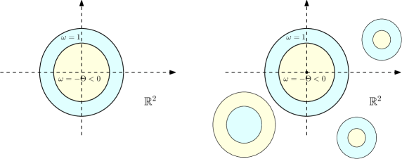
Figure 1: One can choose $\Theta$ so that the radial vorticity has zero average (left). Since the support of such velocity and vorticity coincide, one can place such solutions to produce non-radial solutions (right).

Theorem 1.4 (Corollary 4.5, Theorem 4.27)

There exist vortex patch solutions to the 2D Euler equation (1.1) that are not locally radial, with finite kinetic energy and analytic boundary. Furthermore, the solutions have compactly supported velocity.

Remark 1.5

In this paper, we construct patch-type solutions with compactly supported velocity. This is a consequence of the existence of stationary solutions with finite kinetic energy and our key Lemma 4.3. We note that a smooth stationary solution with finite kinetic energy also has compactly supported velocity (see Remark 4.6).

1.1 2D Euler rigidity and construction of stationary solutions

In this subsection we will summarize some of the history of stationary solutions, mostly focusing on the rigidity (only trivial solutions exist) vs flexibility (non-trivial solutions exist) dichotomy. The first result goes back to Fraenkel [40, Chapter 4], who proved that if $D$ is a stationary, simply connected patch, then $D$ must be a disk. The main idea uses the fact that in this setting, the stream function $\psi=1_{D}*\mathcal{N}$ solves a semilinear elliptic equation $\Delta\psi=g(\psi)$ in $\mathbb{R}^{2}$ with $g(\psi)=1_{\{\psi<C\}}$, and one can apply the moving plane method developed in [79, 47] using the monotonicity of $g$ to obtain the symmetry of $\psi$. However, this result does not cover the non simply-connected case due to the fact that $\psi$ may take different values on the different parts of the boundary and thus one can not apply moving plane techniques. This was solved by the authors and Yao in [51] using a variational approach that does not require this condition, and generalized to the smooth case as long as the vorticity is non-negative. Fraenkel’s result (and method) was generalized to other classes of active scalar equations such as the generalized SQG (where the velocity in (1.1) is given by the perpendicular gradient of the convolution with $\frac{1}{|x|^{\alpha}}$ as opposed to the Newtonian potential) by Reichel [77, Theorem 2], Lu–Zhu [69] and Han–Lu–Zhu [55] in the case of $\alpha\in[0,1)$ and Choksi–Neumayer–Topaloglu [26] in the case $\alpha\in[0,\frac{5}{3})$. In [51] we closed the problem for the full range $\alpha\in[0,2)$.

In the last few years, there has been an emergence of results on rigidity conditions, namely under which hypotheses we can guarantee that the solution has some rigid features in order to ultimately characterize stationary solutions by other geometric properties (such as being a shear or being radial). These are usually referred as ‘Liouville” type of results. In the case of 2D Euler, Hamel–Nadirashvili in [54, 52] proved that any stationary solution without a stagnation point must be a shear flow whenever the domain is a strip and also in [53] proved the corresponding rigidity (radial symmetry) result whenever the domain is a two-dimensional bounded annulus, an exterior circular domain, a punctured disk or a punctured plane. Constantin–Drivas–Ginsberg [29, 28] obtained rigidity and flexibility results for Euler and other equations (such as MHD) in both 2D and 3D. Coti-Zelati–Elgindi–Widmayer [32] constructed stationary solutions close to the Kolmogorov and Poiseuille flows in $\mathbb{T}^{2}$. In the case of 2D Navier–Stokes, Koch–Nadirashvili–Seregin–Šverák also proved a Liouville theorem in [66]. See also [49, 50] where together with Yao we proved rigidity and flexibility results for the vortex sheet problem.

We now review some additional results related to the characterization or construction of nontrivial stationary solutions to 2D Euler (flexibility). Nadirashvili [74], following Arnold [2, 3, 4] studied the geometry and the stability of stationary solutions. When the problem is posed on a surface, Izosimov–Khesin [63] characterized stationary solutions of 2D Euler. Choffrut–Šverák [22] showed that locally near each stationary smooth solution there exists a manifold of stationary smooth solutions transversal to the foliation, and Choffrut–Székelyhidi [23] showed that there is an abundant set of stationary weak ($L^{\infty}$) solutions near a smooth stationary one. Shvydkoy–Luo [70, 71] looked at stationary smooth solutions of the form $v=\nabla^{\perp}(r^{\gamma}f(\omega))$, where $(r,\omega)$ are polar coordinates and were able to obtain a classification of them. In a different direction, Turkington [82] used variational methods to construct stationary vortex patches of a prescribed area in a bounded domain, imposing that the patch is a characteristic function of the set $\{\Psi>0\}$, and also studied the asymptotic limit of the patches tending to point vortices. He also studied the case of unbounded domains. We emphasize that those solutions do not have finite energy, unless the domain is bounded. Long–Wang–Zeng [68] studied the regularity in the smooth setting (see also [14]) as well as their stability. For other variational constructions close to point vortices, we would like to mention the work done by Cao–Liu–Wei [12], Cao–Peng–Yan [13] and Smets–van Schaftingen [81]. Musso–Pacard–Wei [73] constructed nonradial smooth stationary solutions with finite energy but without compact support in $\omega$. Our solutions are different from all of these constructions since they are not close to point vortices.

The (nonlinear $L^{1}$) stability of circular patches was proved by Wan–Pulvirenti [83] and later Sideris–Vega gave a shorter proof [80]. See also Beichman–Denisov [6] for similar results on the strip. Recently, Choi–Lim [25] generalized the stability results for radial patches to radially symmetric monotone vorticity. Lately, Gavrilov [45, 46] managed to construct nontrivial stationary solutions of 3D Euler with compactly supported velocity, which was further simplified and extended to other equations by Constantin–La–Vicol [30]. In [39], Domínguez-Vázquez–Enciso–Peralta-Salas construct a different family of non-localizable, stationary solutions of 3D Euler that are axisymmetric with swirl. Regarding the stability results in 3D, we refer to the work of Choi [24] for solutions near Hill’s spherical vortex.

1.2 Structure of the proofs

The skeleton of our proof employs bifurcation theory, trying to find a perturbation of trivial solutions (radial vorticity). A very natural procedure is to frame it using a Crandall-Rabinowitz Theorem approach (see [18, 19, 16, 17, 20, 41, 42, 44, 43, 48, 56, 58, 36, 59, 57] for applications in the context of fluid mechanics). In a suitable functional setting, the problem boils down to finding non-trivial zeros of a nonlinear functional of the form (see (2.3)) :

$$\mathcal{F}(\Theta,R)=0,\quad F:\mathbb{R}\times H^{k+1}(\mathbb{T})\mapsto H^{k}(\mathbb{T}),\quad k\geq 3,\text{ given that $\mathcal{F}(\Theta,0)=0$ for any $\Theta\in\mathbb{R}$}.$$

Note that the loss of derivatives attributes to the fact that each component of the functional in (2.3) takes account of the tangent vector of the boundaries. An easy observation is that the non-degeneracy of the velocity at the trivial solution (more precisely, the angular velocity $\neq 0$) guarantees that the linearized functional is Fredholm. For a radial vorticity with infinite energy, this can be more explicitly revealed in the linearized operators obtained in Proposition 3.6, where the the angular velocity contributes to the diagonal elements of the matrix $M_{n}$, which can also be seen in (4.5). However, for a radial vorticity whose average vanishes, the corresponding velocity field, which can be explicitly computed, vanishes outside the support of the vorticity. At such trivial solutions, the linearized functional fails to be Fredholm and one cannot directly apply the Crandall-Rabinowitz Theorem. Indeed, the degeneracy of the velocity on the outmost boundary yields a mismatch of the image spaces of the functional at the nonlinear level and the linear level in terms of the regularity. One possible attempt to overcome this issue is to find two bifurcation curves emanating from negative-average vorticity and positive-average vorticity that are close to each other and show that the two curves merge together forming a loop, using the strategy in [60] (see Figure 2). It is not difficult to find (in the three-layer setting) values for $\Theta^{+}$ and $\Theta^{-}$ and doing numerical continuation one can observe those loops.

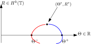
Figure 2: One possible strategy: Find two bifurcation curves emanating from negative average and positive average and show that those two curves are connected. If it is possible, then there must be a solution with zero-average $(\Theta^{*},R^{*})$ by continuity.

Our key Lemma 4.3 shows that the degeneracy of the velocity is not a special case at the trivial solutions, but a generic phenomenon. More precisely, if the vorticity $\omega$ is stationary (not necessarily radial) with zero-average, then $u=0$ outside the support of $\omega$ as long as $\text{supp}(\omega)$ is simply connected. This gives two crucial implications:

• A non-trivial stationary solution near a trivial one cannot be obtained by using the implicit function theorem. In Figure 2, $D_{R}\mathcal{F}(\Theta^{*},R^{*})$, the linearized operator at $(\Theta^{*},R^{*})$ (if it exists) cannot be an isomorphism.

• The mismatch in regularity between the image spaces described above may be treated in the sprit of Nash-Moser scheme with the use of an approximate inverse.

The first implication shows that one cannot use the Lyapunov-Schmidt reduction which is a crucial tool in the strategy in [60] to find a loop of bifurcation curves and even more importantly in the original proof of the Crandall-Rabinowitz theorem. Regarding the second implication, the Nash-Moser scheme has been well-adapted in the context of steady-state solutions [22, 61, 62], dynamical solutions [67, 78] and more recently, embedded into a KAM scheme in the context of quasiperiodic solutions for the water waves problem (see [5] and the references therein). In Section 4, we will find a bifurcation curve without the use of such a reduction technique, and combine it with the Nash-Moser scheme in the following way:

• In Subsection 4.1, we slightly modify our functional setting given in Section 2 so that $(\Theta,R)$ represents a zero-average vorticity. We are led to find non-trivial zeros of the modified functional (see (4.5) for the definition of $G$)

  $$G:\mathbb{R}\times H^{k+1}\mapsto H^{k},\quad\text{given that ${G}(\Theta,0)=0$ for any $\Theta\in\mathbb{R}$ }.$$

  See also (4.161), where it is shown that each component of $G$ is the tangential derivative of the stream function on each boundary component.

• We analyze the linearized operator $D_{R}G$ to find $\Theta^{*}\in\mathbb{R}$ such that $D_{R}G(\Theta^{*},0)$ satisfies (Subsection 4.5.4)

  • Ker$(D_{R}G(\Theta^{*},0))$ is one-dimensional, that is, Ker$(D_{R}G(\Theta^{*},0))=\text{span}\left\{v\right\}$ for some $v\in C^{\infty}$.

  • Im$(D_{R}G(\Theta^{*},0))^{\perp}$ is one-dimensional.

  • $(D_{R}G(\Theta^{*},0))$ satisfies the transversality condition: $\partial_{\Theta}D_{R}(G(\Theta^{*},0))[v]\notin\text{Im}D_{R}G(\Theta^{*},0)$.

  This indicates that a possible non-trivial solution can be found as a zero of the following functional for sufficiently small $s>0$:

  $$\tilde{G}_{s}:H^{k+1}\mapsto H^{k},\quad\tilde{G}_{s}(R):=G(\Theta^{*}+v\cdot R,sv+(I-P)[R]),$$ (1.2)

  where $P:H^{k+1}\mapsto C^{\infty}$ is the projection to $\text{Ker}(D_{R}G(\Theta^{*},0))$, and $I$ is the identity operator (see (4.19)).

• We perform Newton’s method for the functional $\tilde{G}_{s}$. The two important ingredients for Newton’s method to work are 1) a sufficiently good initial guess and 2) the invertibility of the linearized operator $D\tilde{G}_{s}$. For the initial guess, we already have $\tilde{G}_{s}=O(s^{2})$, since $v\in\text{Ker}(D_{R}G(\Theta^{*},0))$.

• Regarding the second ingredient, we observe that the operator $D_{R}G(\Theta,R)$ can be decomposed

  $$D_{R}G=a+A\text{ as in \eqref{decomp_11},}$$

  where the operator $a(\Theta,R)$ vanishes if $(\Theta,R)$ corresponds to a stationary solution. This is due to the fact that the velocity on the outmost boundary vanishes by Lemma 4.3. This observation leads us to decompose $D\tilde{G}_{s}$, which can be immediately computed from (1.2) as

  $$D\tilde{G}_{s}=\partial_{\Theta}G\circ P+D_{R}G\circ(I-P)=\underbrace{\partial_{\Theta}G\circ P+A\circ(I-P)}_{=:T_{s}}+a\circ(I-P),\quad\text{ see \eqref{T_sdef}}.$$

  Thanks to the transversality condition, the one dimensionality of $\text{Im}(D_{R}G(\Theta^{*},0))^{\perp}(=\text{Im}A(\Theta^{*},0)^{\perp}$ since $a(\Theta^{*},0)=0$) is compensated by $\partial_{\Theta}G\circ P$. Indeed, it is the main goal of Subsection 4.3.1 to show that $T_{s}$ is invertible.

• As described in 4) we do not have the invertibility of $D\tilde{G}_{s}$, however, the invertibility of $T_{s}$ is enough for the iteration in (4.58) to work since $a$ tends to $0$ along the iteration steps towards the solution. More precisely, $T_{s}$ plays a role of the approximate inverse of $D\tilde{G}_{s}$. The loss of derivatives occurring at each iteration step is treated by the use of regularizing operator in (4.57) in the spirit of the Nash-Moser scheme.

We note that our finite energy solutions consist of three-layered vortex patches, unlike the infinite energy case (See Subsection 3.1 and 4.1). From the technical point of view, the two-layered, zero-average trivial solutions do not give a linearized operator that has finite dimensional Kernel. More precisely, one cannot find a pair of parameters $(b,\Theta)$ such that 1) the matrix $M_{n}$ in Proposition 3.6 has zero-determinant and 2) the corresponding $\omega$ determined by $(b,\Theta)$ has zero-average (see Remark 3.12). An important aspect of such two-layered stationary vorticity is that its stream function $\psi$ always satisfies

$$\Delta\psi=g(\psi),\text{ for some $g:\mathbb{R}\mapsto\mathbb{R}$}.$$ (1.3)

We emphasize that the solutions that we construct in this paper cannot be captured by (1.3) unlike the earlier works, for example, [81, 32, 28]. That is, there is no $g$ such that the stream function $\psi$ solves (1.3). This feature can been seen from the fact that the trivial solutions from which we bifurcate to obtain finite energy solutions exhibit non-monotone stream functions in the radial direction.

Lastly, we point out that the desingularization from point vortices is not applicable to find a stationary solution with finite energy, since a steady configuration of point vortices has zero vortex angular momentum, which together with the finite energy hypothesis implies that the individual circulations have to be all zero (see [75, Lemma 1.2.1]).

1.3 Organization of the paper

The paper is organized in the following way: Section 2 sets up the functional framework and the equation that a stationary solution has to satisfy. Section 3 proves Theorem 1.2, in the easier case where the finite energy hypothesis is dropped. Finally, section 4 proves Theorem 1.4 in the full generality setting using the Nash-Moser scheme. The Appendix contains some technical background results used throughout the proof, as well as basic bifurcation theory and some integrals needed for the spectral study.

2 Functional equations and functional setting for stationary vortex patches

Let us consider vorticity $\omega$ of the form $\omega:=\sum_{i=1}^{n}\Theta_{i}1_{D_{i}}$ for some $n\in\mathbb{N}$, where $\Theta_{i}\in\mathbb{R}$ and $D_{i}$ is a simply-connected domain for each $i=1,\ldots,n$. Suppose the boundary of $D_{i}$ is parametrized by a time-dependent $2\pi$-periodic curve $z_{i}(\cdot,t):\mathbb{T}\mapsto\mathbb{R}^{2}$. The evolution equation of the boundary can be written as a system of equations,

$$\partial_{t}z_{j}(x,t)\cdot\partial_{x}z_{j}(x,t)^{\perp} =u(z_{j}(x,t),t)\cdot\partial_{x}z_{j}(x,t)^{\perp}.$$ (2.1)

where $u(\cdot,t):=\nabla^{\perp}\left(\omega(\cdot,t)*\frac{1}{2\pi}\log|\cdot|\right)$ is the velocity vector. We will look for stationary solutions to $\eqref{evolution_patch}$. Let us assume that each $z_{i}$ can be written as

$$z_{i}(x)=(b_{i}+R_{i}(x))(\cos(x),\sin(x)),\quad x\in\mathbb{T},$$ (2.2)

where $b_{i}$ is a positive constant for each $i$. By plugging these parametrizations into (2.1), we are led to solve the following system for $b:=(b_{1},\ldots,b_{n})$, $\Theta:=(\Theta_{1},\ldots,\Theta_{n})$ and $R:=(R_{1},\ldots,R_{n})$:

$$0=\mathcal{F}_{j}(b,\Theta,R):=u(z_{j}(\cdot))\cdot z_{j}^{\prime\perp} :=\sum_{i=1}^{n}\frac{1}{4\pi}\Theta_{i}u_{i,j}(R)\cdot z_{j}^{\prime\perp}=\sum_{i=1}^{n}\frac{1}{4\pi}\Theta_{i}\underbrace{\left(u_{i,j}^{\theta}(R)R_{j}^{\prime}-u_{i,j}^{r}(R)(b_{j}+R_{j})\right)}_{=:S_{ij}(b_{i},b_{j},R_{i},R_{j})}.$$ (2.3)

where $u_{i,j}(R)(x):=\nabla^{\perp}\left(1_{D_{i}}*\log|\cdot|^{2}\right)(z_{j}(x))$, which can be thought of as a contribution of the $i$th patch on the $j$th curve, and $u_{i,j}^{\theta}$ and $u_{i,j}^{r}$ are the angular and the radial components of $u_{i,j}$. More explicitly, we have

$$S_{ij}(b_{i},b_{j},R_{i},R_{j}) =\int_{0}^{2\pi}\cos(x-y)((b_{i}+R_{i}(y))R_{j}^{\prime}(x)-(b_{j}+R_{j}(x))R_{i}^{\prime}(y))$$

$$\times\log((b_{j}+R_{j}(x))^{2}+(b_{i}+R_{i}(y))^{2}-2(b_{j}+R_{j}(x))(b_{i}+R_{i}(y))\cos(x-y))dy$$

$$-\int_{0}^{2\pi}\sin(x-y)((b_{i}+R_{i}(y))(b_{j}+R_{j}(x))+R_{i}^{\prime}(y)R_{j}^{\prime}(x))$$

$$\times\log((b_{j}+R_{j}(x))^{2}+(b_{i}+R_{i}(y))^{2}-2(b_{j}+R_{j}(x))(b_{i}+R_{i}(y))\cos(x-y))dy.$$ (2.4)

It is clear that $S_{ij}(b_{i},b_{j},0,0)=0,$ since $u_{i,j}^{r}=0$ for radial patches. Thus we have

$$\mathcal{F}(b,\Theta,0)=0,\text{ for any $b,\Theta$.}$$ (2.5)

In what follows, we will pick one of $\Theta_{i}$ as a bifurcation parameter, while the others are fixed.

We now proceed to discuss the functional spaces that we will use. In Section 3 we will work with the following analytic spaces. Following [17], we denote the space of analytic functions in the strip $\left\{z\in\mathbb{C}:\text{Im}(z)\leq c\right\}$ by $\mathcal{C}_{w}(c)$. For $k\in\mathbb{Z}$, we will consider the following spaces of $\frac{2\pi}{m}$-periodic functions:

$$X^{k,m}_{c}:=\left\{f(x)\in\mathcal{C}_{w}(c),\quad f(x)=\sum_{j=1}^{\infty}a_{jm}\cos(jmx),\quad\rVert f\rVert_{X^{k,m}_{c}}<\infty\right\},$$

$$Y^{k,m}_{c}:=\left\{f(x)\in\mathcal{C}_{w}(c),\quad f(x)=\sum_{j=1}^{\infty}a_{jm}\sin(jmx),\quad\rVert f\rVert_{Y^{k,m}_{c}}<\infty\right\},$$

where $\rVert f\rVert_{X^{k,m}_{c}}=\rVert f\rVert_{Y^{k,m}_{c}}:=\sum_{j=1}^{\infty}|a_{jm}|^{2}(1+jm)^{2k}(\cosh(cjm)^{2}+\sinh(cjm)^{2})$.

In Section 4 we will consider the following spaces of $\frac{2\pi}{m}$-periodic functions:

$$X^{k,m}:=\left\{f(x)\in H^{k}(\mathbb{T}):\quad f(x)=\sum_{j=1}^{\infty}a_{jm}\cos(jmx),\quad\rVert f\rVert_{X^{k,m}}<\infty\right\},$$

$$Y^{k,m}:=\left\{f(x)\in H^{k}(\mathbb{T}):\quad f(x)=\sum_{j=1}^{\infty}a_{jm}\sin(jmx),\quad\rVert f\rVert_{Y^{k,m}}<\infty\right\},$$

where $\rVert f\rVert_{X^{k,m}}=\rVert f\rVert_{Y^{k,m}}:=\rVert f\rVert_{H^{k}(\mathbb{T})}$.

3 Warm-up: Existence of non-radial stationary vortex patches with infinite energy

As a warm-up, in this section we aim to show that there exists a non-trivial patch solution with infinite kinetic energy, $\frac{1}{2\pi}\int_{\mathbb{R}^{2}}|\nabla\left(\omega*\log|\cdot|\right)|^{2}dx=\infty$. Recall that ([72, Proposition 3.3]),

$$\int_{\mathbb{R}^{2}}|\nabla\left(\omega*\log|\cdot|\right)|^{2}dx<\infty\iff\int_{\mathbb{R}^{2}}\omega(x)dx=0.$$ (3.1)

In our proof, we will find a continuous bifurcation curve, emanating from a two-layered vortex patch whose vorticity does not has zero mean.

3.1 Main results for infinite energy

Let us consider two-layer vortex patches, that is, $i\in\left\{1,2\right\}$ in the setting in Section 2. For $b,\Theta\in(0,1)$, using the scaling invariance of the equations, we will choose the parameters to be

$$b_{1}=1,\quad b_{2}=b,\quad\Theta_{1}=\Theta,\quad\Theta_{2}=-1,$$ (3.2)

so that if $R_{1}=R_{2}=0$, then

$$\omega=\begin{cases}\Theta&\text{ in }B_{1}\backslash B_{b}\\ \Theta-1&\text{ in }B_{b},\end{cases}$$ (3.3)

where $B_{r}$ denotes the unit disk centered at the origin. Note that the case $\Theta=1$ corresponds to an annulus. Later, we will fix $b$ as well, and let $\Theta$ play the role as a bifurcation parameter. With this setting, the system (2.3) is equivalent to

$$0=\mathcal{F}(\Theta,R)=(F^{1}(\Theta,R),F^{2}(\Theta,R)),\quad R=(R_{1},R_{2}),$$ (3.4)

where we omit the dependence of $\Theta_{2}$ and $b_{1}$, $b_{2}$ for notational simplicity.

Theorem 3.1

Let $k,m$ be such that $k\geq 3$, $2\leq m\in\mathbb{N}$. Let $b$ satisfy the condition in Lemma 3.8. Then for some $c>0$ and $s_{0}=s_{0}(k,m,c,b)>0$, there exist two bifurcation curves $[0,s_{0})\ni s\mapsto(\Theta^{\pm}(s),R^{\pm}(s))\in\mathbb{R}\times(X^{k,m}_{c})^{2}$ such that for each $s\in(0,s_{0})$, $(\Theta^{\pm}(s),R^{\pm}(s))$ is a solution of the equation (3.4) and $R^{\pm}(s)\neq 0\in(X^{k,m}_{c})^{2}$. The bifurcation curve emanates from $(\Theta^{\pm}(0),R^{\pm}(0))=(\Theta_{m}^{\pm},0)$, where $\Theta_{m}^{\pm}$ are defined in Lemma 3.8.

Theorem 3.1 immediately implies the existence of non-radial stationary vortex patches with infinite energy.

Corollary 3.2

Let $2\leq m\in\mathbb{N}$. Then there is an $m$-fold symmetric stationary patch solution for the 2D Euler equation with analytic boundary and infinite kinetic energy, that is

$$\int_{\mathbb{R}^{2}}|\nabla\left(\omega*\frac{1}{2\pi}\log|\cdot|\right)|^{2}dx=\infty.$$

Proof.

By Theorem 3.1, there are two continuous bifurcation curves $\Psi^{\pm}:[0,s_{0})\mapsto\mathbb{R}\times\left(X^{k,m}_{c}\right)^{2}$ of solutions of (3.4) such that

$$\Psi^{\pm}(s)=\left(\Theta^{\pm}(s),R(s)\right),\quad F(\Psi^{\pm}(s))=0,\quad\text{ and }\quad\Psi^{\pm}(0)=\left(\Theta_{m}^{\pm},0\right),$$

for some $s_{0}>0$. From (2.1) and (2.3), it is clear that for each $s\in(0,s_{0})$ and for each choice of $\pm$,

$$\omega^{s}(x):=\begin{cases}\Theta-1&\text{ if }x\in D_{2}(s),\\ \Theta&\text{ if }x\in D_{1}(s)\backslash\overline{D_{2}(s)}\\ 0&\text{ otherwise, }\end{cases}$$ (3.5)

is a stationary solution to the Euler equation, where $D_{1}(s)$ and $D_{2}(s)$ are the bounded domains determined by (2.2) with $R(s)$. Since $R(s)\in\left(X^{k,m}_{c}\right)^{2}$, the boundaries are analytic.

Now we consider the kinetic energy of the solution. From (3.1), it suffices to show that $\int_{\mathbb{R}^{2}}\omega^{0}(x)dx\neq 0$. By the continuity of the bifurcation curve, this immediately implies that $\int_{\mathbb{R}^{2}}\omega^{s}(x)dx\neq 0$ for small $s>0$. Then it follows from Lemma 3.11 that $b^{2}<\Theta_{m}^{\pm}$, hence

$$\int_{\mathbb{R}^{2}}\omega^{0}(x)dx=\pi\left(-b^{2}+\Theta_{m}^{\pm}\right)>0.$$

This completes the proof. ∎

The rest of this section will be devoted to prove Theorem 3.1. The proof will be divided into 5 steps. These steps correspond to check the hypotheses of the Crandall-Rabinowitz theorem A.1 for our functional $F$ in (3.4). The hypotheses in Theorem A.1 can be read as follows in our setting:

1. The functional $\mathcal{F}$ satisfies

   $$\mathcal{F}(\Theta,R)\,:\,(0,1)\times\{V^{\epsilon}\}\mapsto(Y^{k-1,m}_{c})^{2},$$

   where $V^{\epsilon}$ is an open neighborhood of 0,

   $$V^{\epsilon}=\left\{(f,g)\in(X^{k,m}_{c})^{2}\,:\,||f||_{X^{k,m}_{c}}+||g||_{X^{k,m}_{c}}<\epsilon\right\}$$

   for some $\epsilon>0$ and $k\geq 3$.

2. $\mathcal{F}(\Theta,0)=0$ for every $0<\Theta<1$.

3. The partial derivatives $\partial_{\Theta}\mathcal{F}$, $D\mathcal{F}$, $\partial_{\Theta}D\mathcal{F}$ exist and are continuous, where $D\mathcal{F}$ is Gateaux derivative of $\mathcal{F}$ with respect to the functional variable $R$.

4. Ker$(D\mathcal{F}(\Theta_{m}^{\pm},0))\subset(X^{k,m}_{c})^{2}$ and $(Y^{k-1,m}_{c})^{2}$/Im($D\mathcal{F}(\Theta_{m}^{\pm},0)$) are one-dimensional (see Proposition 3.8 for the definition of $\Theta_{m}^{\pm}$).

5. $\partial_{\Theta}D\mathcal{F}(\Theta_{m}^{\pm},0)[v_{0}]\not\in$ Im($D\mathcal{F}(\Theta_{m}^{\pm},0)$), where $v_{0}$ is a non-zero element in Ker$(D\mathcal{F}(\Theta_{m}^{\pm},0))$.

Remark 3.3

We remark that if $i\neq j$ then the functions inside the logarithm in $S_{i,j}$ in (2) are uniformly bounded from below in $y$ for all $x$ by a strictly positive constant depending on the parameters. Then we can analytically extend the integrand in $x$ to the strip $|\Im(z)|\leq c$ in such a way that the real part of this extension stays uniformly bounded away from 0 for a small enough $c$. The case $i=j$ can be treated similarily as in [17, Remark 2.1].

3.2 Proof of Theorem 3.1

3.2.1 Steps 1,2 and 3: Regularity

In order to check the first three steps, it suffices to check if $S_{ij}$ in (2) satisfies the hypotheses, since $F$ is a linear combination of $S_{ij}$. As mentioned in Remark 3.3, the case $i\neq j$ is trivial since there is no singularity in the integrand and analytically extended into a strip in $\mathbb{C}$, if $(R_{1},R_{2})$ is in a sufficiently small neighborhood of $(0,0)$. For $i=j$, the first three steps with slightly different settings were already done in the literature. For example, step 1 can be done in the same way as in [35]. Step 2 follows immediately from (2.5). Existence and continuity of the Gateaux derivatives for the gSQG equation was done in [48] and the same proof can be adapted to our setting straightforwardly.

3.2.2 Step 4: Analysis of the linear part.

In this section, we will focus on the spectral study of the Gateaux derivative $D\mathcal{F}(\Theta,0):=D_{R}\mathcal{F}(\Theta,0)$.

Calculation of $D\mathcal{F}$

We aim to express the Gateaux derivative of $\mathcal{F}$ around $(\Theta,0)$ in the direction $(H(x),h(x))$ in terms of Fourier series.

Lemma 3.4

Let $S_{ij}$ be defined as in (2). Then:

$$\left.\frac{d}{dt}S_{ij}(b_{i},b_{j},th_{i},th_{j})\right|_{t=0} =\int b_{i}(h_{j}^{\prime}(x)\cos(x-y)-h_{i}^{\prime}(y))\log(b_{j}^{2}+b_{i}^{2}-2b_{j}b_{i}\cos(x-y))dy=:\mathcal{L}_{1}+\mathcal{L}_{2}.$$

Proof.

Let $V^{1,ab}_{ij}$ (resp. $V^{2,ab}_{ij}$) be the contribution of the first term (resp. second term) of (2) where the first factor contributes with a $t^{a}$ and the second with $t^{b}$. We are looking for all combinations such that $a+b=1$. We start looking at the first summand. We have that:

$$V_{ij}^{1,10} =\int\cos(x-y)(b_{i}h_{j}^{\prime}(x)-b_{j}h_{i}^{\prime}(y))\log(b_{j}^{2}+b_{i}^{2}-2b_{j}b_{i}\cos(x-y))dy.$$

Similarly, for the second one,

$$V_{ij}^{2,01} =-2\int\sin(x-y)(b_{i}b_{j})\frac{h_{j}(x)(b_{j}-b_{i}\cos(x-y))+h_{i}(y)(b_{i}-b_{j}\cos(x-y))}{b_{j}^{2}+b_{i}^{2}-2b_{j}b_{i}\cos(x-y)}dy,$$

$$V_{ij}^{2,10} =-\int\sin(x-y)(b_{i}h_{j}(x)+b_{j}h_{i}(y))\log(b_{j}^{2}+b_{i}^{2}-2b_{j}b_{i}\cos(x-y))dy,$$

where we have used Lemma A.2. Integrating by parts in $V_{ij}^{2,01}$:

$$V_{ij}^{2,01} =\int((b_{i}h_{j}(x)+b_{j}h_{i}(y))\sin(x-y)-h_{i}^{\prime}(y)(b_{i}-b_{j}\cos(x-y)))\log(b_{j}^{2}+b_{i}^{2}-2b_{j}b_{i}\cos(x-y))dy,$$

Finally, adding all the log terms and the non-log terms together:

$$V_{ij}^{1,10}+V_{ij}^{2,01}+V_{ij}^{2,10} =\int b_{i}(h_{j}^{\prime}(x)\cos(x-y)-h_{i}^{\prime}(y))\log(b_{j}^{2}+b_{i}^{2}-2b_{j}b_{i}\cos(x-y))dy,$$

as we wanted to prove. ∎

Lemma 3.5

Let $h_{i}=A_{i}\cos(mx)$ and $r=\frac{\min\{b_{i},b_{j}\}}{\max\{b_{i},b_{j}\}}$. Then:

$$\left.\frac{d}{dt}S_{ij}(b_{i},b_{j},th_{i},th_{j})\right|_{t=0}=2\pi\sin(mx)mb_{i}\left(A_{j}r-A_{i}\frac{r^{m}}{m}\right).$$

Proof.

From Lemma 3.4 and Corollary A.4, we have that

$$\mathcal{L}_{1} =-mb_{i}A_{j}\sin(mx)\mathcal{A}_{0}(r,1),$$

$$\mathcal{L}_{2} =mb_{i}A_{i}\sin(mx)\mathcal{A}_{0}(r,m),$$

Adding the two contributions gives the desired result. ∎

Note that the functional $\mathcal{F}$ is a linear combination of $S_{ij}$ (see (2.3)). Using the above two lemmas, we obtain the following proposition:

Proposition 3.6

Let $h(x)=\sum_{n}a_{n}\cos(nx),$ $H(x)=\sum_{n}A_{n}\cos(nx)$, then we have that:

$$D\mathcal{F}(\Theta,0)[H,h]=\left(\begin{array}[]{c}U(x)\\ u(x)\end{array}\right),$$

where

$$U(x)=\sum_{n}U_{n}\sin(nx),\quad u(x)=\sum_{n}u_{n}\sin(nx),$$

and the coefficients satisfy, for any $n$:

$$\left(\begin{array}[]{c}U_{n}\\ u_{n}\end{array}\right):=(-n)M_{n}(\Theta)\left(\begin{array}[]{c}A_{n}\\ a_{n}\end{array}\right):=(-n)\left(\begin{array}[]{cc}\frac{b^{2}}{2}-\frac{\Theta}{2}+\frac{\Theta}{2n}&-\frac{b^{n+1}}{2n}\\ \Theta\frac{b^{n}}{2n}&-\frac{b}{2n}+\frac{b}{2}(1-\Theta)\end{array}\right)\left(\begin{array}[]{c}A_{n}\\ a_{n}\end{array}\right).$$

Proof.

It follows from (3.2), the definition of $\mathcal{F}$ in (3.4), (2.3) and Lemma 3.5. ∎

One dimensionality of the Kernel of the linear operator.

Our goal here is to verify the one dimensionality of Ker($D\mathcal{F}(\Theta,0)$) for some $\Theta$. More precisely, we will prove the following proposition:

Proposition 3.7

Fix $2\leq m\in\mathbb{N}$ and take any $b\in(0,b_{m})$, where $b_{m}$ is as in Lemma 3.8. Then there exist two $\Theta_{m}^{\pm}\in(0,1)$, such that Ker$(D\mathcal{F}(\Theta_{m}^{\pm},0))$ is one-dimensional. Furthermore,

$$\text{Ker}(D\mathcal{F}(\Theta_{m}^{\pm},0,0))=\text{span}\left\{v_{0}(\Theta_{m}^{\pm})\cos(mx):=\begin{pmatrix}\frac{1}{2m}b-\frac{b}{2}(1-\Theta_{m}^{\pm})\\ \frac{\Theta_{m}^{\pm}}{2m}b^{m}\end{pmatrix}\cos(mx)\right\}\subset X^{k,m}_{c}\times X^{k,m}_{c}.$$

The proof of the above proposition relies on the analysis of the matrix $M_{n}$ in Lemma 3.8 and 3.9, which we will prove below.

Lemma 3.8

Let $\Delta_{m}(\Theta)$ be

$$\Delta_{m}(\Theta):=\frac{4m^{2}}{b}\text{det}(M_{m}(\Theta))=\left(\Theta b^{2m}+b^{2}m(m(1-\Theta)-1)+\Theta(1-m)(m(1-\Theta)-1)\right)$$ (3.6)

Then, for any $m\geq 2$, there exists $0<b_{m}<1$ such that for any $0<b<b_{m}<1$, there exists $0<\Theta^{-}_{m}<\Theta^{+}_{m}<1$ such that $\Delta_{m}(\Theta_{m}^{\pm})=0$. We also have that rk$(M_{m}(\Theta_{m}^{\pm}))=1$ for those values of $\Theta^{+}_{m}$, $\Theta^{-}_{m}$, where $rk(A)$ is the rank of a matrix $A$.

Proof.

For fixed $m$, we study the polynomial $\Delta_{m}(\Theta)$. We need to solve

$$\Delta_{m}(\Theta)=m(m-1)\Theta^{2}-((m-1)^{2}+b^{2}m^{2}-b^{2m})\Theta+b^{2}m(m-1)=0.$$ (3.7)

Since $\Delta_{m}(\Theta)$ is a quadratic function, we only need to show that the discriminant is positive. We have

$$D_{m}:=((m-1)^{2}+b^{2}m^{2}-b^{2m})^{2}-4m^{2}(m-1)^{2}b^{2}$$

$$=((m-1)^{2}+b^{2}m^{2}-b^{2m}-2m(m-1)b)((m-1)^{2}+b^{2}m^{2}-b^{2m}+2m(m-1)b)$$

$$=(m-1-bm-b^{m})(m-1-bm+b^{m})((m-1)^{2}+b^{2}m^{2}-b^{2m}+2m(m-1)b)$$

$$=:D_{m,1}\cdot D_{m,2}\cdot D_{m,3}.$$

Since $m\geq 2$, $0<b<1$, we have $D_{m,3}>1-1=0$. We also have

$$D_{m,2}=m(1-b)+b^{m}-1=(1-b)[m-\frac{1-b^{m}}{1-b}]=(1-b)(m-(1+b+b^{2}+...+b^{m-1}))>0.$$

$D_{m,1}$ is decreasing in $b$ when $b\geq 0$ and $D_{m,1}(0)=m-1>0$, $D_{m,1}(1)=-2$. Let $b_{m}$ be the only zero point of $D_{m,1}$ in (0,1). If we take $0<b<b_{m}$, we have

$$D_{1,m}>0,D_{m}>0.$$ (3.8)

Hence $\Delta_{m}(\Theta)$ has two different solutions $\Theta_{m}^{-}<\Theta_{m}^{+}$. Moreover, the matrix does not vanish when $b\neq 0$, implying rk$(M_{m}(\Theta_{m}^{\pm}))=1$. Now we are left to show $0<\Theta_{m}^{\pm}<1$. We have

$$\Theta_{m}^{+}\Theta_{m}^{+}=b^{2}<1,$$

and

$$\Theta_{m}^{+}+\Theta_{m}^{-}=\frac{((m-1)^{2}+b^{2}m^{2}-b^{2m})}{m(m-1)}\geq\frac{1-1}{m(m-1)}>0.$$

Hence, $0<\Theta_{m}^{-}<1$ and $0<\Theta_{m}^{+}$. If $\Theta_{m}^{+}\geq 1$, then $\Delta_{m}(1)\leq 0$. However,

$$\Delta_{m}(1)=b^{2m}-mb^{2}-(1-m)$$ (3.9)

$$=(1-b^{2})(m-\frac{1-b^{2m}}{1-b^{2}})$$

$$=(1-b^{2})(m-1-b^{2}-...-b^{2m-2})>0.$$

Therefore $0<\Theta_{m}^{\pm}<1$. ∎

We now show that $\Delta_{jm}(\Theta_{m}^{\pm})\neq 0$ for any $j\neq 1$.

Lemma 3.9

Let $j>1$ and let $\Theta_{m}^{\pm}$ and $\Theta_{jm}^{\pm}$ be defined as in the previous Lemma. Then $\Theta_{jm}^{+}>\Theta_{m}^{+}>\Theta_{m}^{-}>\Theta_{jm}^{-}$. Hence, $M_{jm}(\Theta_{m}^{\pm})$ is non-singular for all $j>1$.

Proof.

Since $\Theta_{m}^{\pm}$ solves the equation

$$\Theta^{2}-\frac{((m-1)^{2}+b^{2}m^{2}-b^{2m})}{m(m-1)}\Theta+b^{2}=0.$$

We only need to show $F(b,m):=\frac{((m-1)^{2}+b^{2}m^{2}-b^{2m})}{m(m-1)}$ is strictly increasing with respect to $m$. We have

$$F(b,m+1)-F(b,m)$$

$$=\frac{(m^{2}+b^{2}(m+1)^{2}-b^{2(m+1)})}{(m+1)m}-\frac{((m-1)^{2}+b^{2}m^{2}-b^{2m})}{m(m-1)}$$

$$=\frac{(m^{2}+b^{2}(m+1)^{2}-b^{2(m+1)})(m-1)-((m-1)^{2}+b^{2}m^{2}-b^{2m})(m+1)}{(m+1)m(m-1)}$$

$$=\frac{b^{2}((m+1)^{2}(m-1)-m^{2}(m+1))+m^{2}(m-1)-(m+1)(m-1)^{2}-b^{2m+2}(m-1)+(m+1)b^{2m}}{(m+1)m(m-1)}$$

$$=\frac{-b^{2}(m+1)+m-1-b^{2m+2}(m-1)+b^{2m}(m+1)}{(m+1)m(m-1)}.$$

Thus

$$F(b,m+1)-F(b,m)>0\Leftrightarrow-b^{2}(m+1)+m-1-b^{2m+2}(m-1)+b^{2m}(m+1)>0$$

$$\Leftrightarrow(1+b^{2})(-1+b^{2m})-(-1+b^{2})(1+b^{2m})m>0\Leftrightarrow-(1+b^{2})(b^{2m-2}+b^{2m-4}...+b^{2}+1)+(1+b^{2m})m>0$$

$$\Leftrightarrow-\sum_{k=1}^{m}b^{2m-2k}-\sum_{k=1}^{m}b^{2k}+(1+b^{2m})m>0\Leftrightarrow\sum_{k=1}^{m}(1-b^{2k})(1-b^{2m-k})>0.$$

It is easy to show the last inequality since $0<b<1$. ∎

• Proof of Proposition 3.7: Let $m\geq 2$ and let $b$, $\Theta_{m}^{\pm}$ be as defined in Lemma 3.8. Assume that $H(x)=\sum_{j}A_{jm}\cos(jmx)$ and $h(x)=\sum_{j}a_{jm}\cos(jmx)$ satisfy

  $$DF(\Theta_{m}^{\pm},0)[H,h]=(0,0).$$

  Then it follows from Proposition 3.6 that

  $$M_{jm}(\Theta_{m}^{\pm})\begin{pmatrix}A_{jm}\\ a_{jm}\end{pmatrix}=\begin{pmatrix}0\\ 0\end{pmatrix}.$$

  For all $j>1$, it follows from Lemma 3.9 that $M_{jm}(\Theta_{m}^{\pm})$ is invertible, thus $A_{jm}=a_{jm}=0$. For $j=1$, Lemma 3.8 tells us that $(A_{m},a_{m})\in\text{Ker}(M_{m}(\Theta_{m}^{\pm}))=\text{span}\left\{v_{0}(\Theta_{m}^{\pm}):=\begin{pmatrix}\frac{1}{2m}b-\frac{b}{2}(1-\Theta_{m}^{\pm})\\ \frac{\Theta_{m}^{\pm}}{2m}b^{m}\end{pmatrix}\right\}$. This finishes the proof. $\Box$

Codimension of the image of the linear operator.

We now characterize the image of $D\mathcal{F}(\Theta_{m}^{\pm},0)$. We have the following proposition:

Proposition 3.10

Let

$$Z=\left\{(Q,q)\in Y^{k-1,m}_{c}\times Y^{k-1,m}_{c},Q(x)=\sum_{j=1}^{\infty}Q_{jm}\sin(jmx),q(x)=\sum_{j=1}^{\infty}q_{jm}\sin(jmx),\right.$$

$$\left.\exists\lambda_{Q,q}\in\mathbb{R}\text{ s.t.}\left(\begin{array}[]{c}Q_{m}\\ q_{m}\end{array}\right)=\lambda_{Q,q}\left(\begin{array}[]{c}-\frac{1}{2m}b^{m+1}\\ -\frac{1}{2m}b+\frac{b}{2}(1-\Theta_{m}^{\pm})\end{array}\right)\right\}.$$

Then $Z=\text{Im}\left(D\mathcal{F}(\Theta_{m}^{\pm},0,0)\right)$.

Proof.

In view of Proposition 3.6, $\text{Im}\left(D\mathcal{F}(\Theta_{m}^{\pm},0)\right)\subset Z$ is trivial, since $M_{jm}(\Theta_{m}^{\pm})$ is non-singular for $j>1$, and $\text{Im}(M_{m}(\Theta_{m}^{\pm}))=\text{span}\left\{\begin{pmatrix}-\frac{1}{2m}b^{m+1}\\ -\frac{1}{2m}b+\frac{b}{2}(1-\Theta)\end{pmatrix}\right\}.$ In order to prove $\text{Im}\left(D\mathcal{F}(\Theta_{m}^{\pm},0)\right)\supset Z$, we need to check whether the possible preimage satisfies the desired regularity. To do so, we have the following asymptotic lemma:

Lemma 3.11

For fixed $m\geq 2$ and $b$ defined as in Proposition 3.7, we have $b^{2}-\Theta_{m}^{\pm}<0$ and

$$\frac{b}{4j^{2}m^{2}}\Delta_{jm}(\Theta_{m}^{\pm})=\frac{b}{4}\left(b^{2}-\Theta_{m}^{\pm}\right)(1-\Theta_{m}^{\pm})+O\left(\frac{1}{jm}\right),\quad\text{ as }j\to\infty,$$ (3.10)

Consequently, we have

$$\text{det}{(M_{jm}(\Theta_{m}^{\pm}))^{-1}}\lesssim_{m,\Theta}1,\quad\text{ for sufficiently large }j.$$ (3.11)

Remark 3.12

As shown in the above lemma, there is no bifurcation curve from the two-layered vortex patch with zero-average. This is due to the fact that the radial vorticity $\omega$ determined by $b$ and $\Theta^{\pm}$ as in (3.3) satisfies $\int_{\mathbb{R}^{2}}\omega dx=\pi\left(-b^{2}+\Theta_{m}^{\pm}\right)>0$. Note that if we require $\Theta=b^{2}$ to ensure $\int\omega dx=0$, it follows from (3.6) that $\Delta_{m}(b^{2})=mb^{2}(1-b^{2})+b^{2}(b^{2m}-1)$, which does not vanish for any $m\geq 2$ unless $b=0$ or $b=1$. Therefore, for any $0<b<1$, the linearized operator is an isomorphism and the implicit function theorem shows that there cannot be a bifurcation.

• Proof of Lemma 3.11: First we show that $b^{2}<\Theta_{m}^{\pm}$. By Lemma 3.8, $\Theta_{m}^{+}\Theta_{m}^{-}=b^{2}$ and $0<\Theta_{m}^{\pm}<1$. Thus $\Theta_{m}^{\pm}>b^{2}$. Therefore the first assertion is proved. The second assertion follows directly from (3.6) since

  $$\frac{b}{4(jm)^{2}}\Delta_{jm}(\Theta_{m}^{\pm})=\frac{b}{4(jm)^{2}}\left((b^{2}-\Theta_{m}^{\pm})(1-\Theta_{m}^{\pm})(jm)^{2}+O\left(m\right)\right)=\frac{b}{4}\left(b^{2}-\Theta_{m}^{\pm}\right)(1-\Theta_{m}^{\pm})+O\left(\frac{1}{jm}\right).$$

  Lastly, by choosing $j$ large so that $|\frac{b}{4(jm)^{2}}\Delta_{jm}(\Theta_{m}^{\pm})|>\frac{b}{8}(\Theta_{m}^{\pm}-b^{2})(1-\Theta_{m}^{\pm})>0$, we have

  $$|\text{det}(M_{jm}(\Theta_{m}^{\pm})^{-1})|=\frac{1}{|\frac{b}{4(jm)^{2}}\Delta_{jm}(\Theta_{m}^{\pm})|}\lesssim 1,$$

  which proves (3.11). $\Box$

Now for an element $(Q,q)\in Z$, let $(H,h)$ be such that

$$H(x)=\sum_{j=1}^{\infty}A_{jm}\cos(jmx),\quad h(x)=\sum_{j=1}^{\infty}a_{jm}\cos(jmx),$$

with

$$\begin{pmatrix}A_{m}\\ a_{m}\end{pmatrix}=-\frac{1}{m}\begin{pmatrix}0\\ \lambda_{Q,q}\end{pmatrix},\quad\begin{pmatrix}A_{jm}\\ a_{jm}\end{pmatrix}=(-jm)^{-1}M_{jm}(\Theta_{m}^{\pm})^{-1}\begin{pmatrix}Q_{jm}\\ q_{jm}\end{pmatrix}\quad\text{ for $j>1$}.$$

It is clear from (3.6) that $D\mathcal{F}(\Theta_{m}^{\pm},0,0)(H,h)=(Q,q).$ We will prove that $(H,h)\in X^{k,m}_{c}\times X^{k,m}_{c}$. From Lemma 3.11 and the fact that $M_{jm}(\Theta_{m}^{\pm})$ is nonsingular for $j>1$, it follows that

$$|A_{jm}|^{2}+|a_{jm}|^{2}\lesssim(jm)^{-2}\left(|Q_{jm}|^{2}+|q_{jm}|^{2}\right)\quad\text{ for all }j>1.$$ (3.12)

Thus, we obtain

$$\rVert H\rVert_{X^{k,m}_{c}}^{2}+\rVert h\rVert_{X^{k,m}_{c}}^{2} =\sum_{j=1}^{\infty}\left(|A_{jm}|^{2}+|a_{jm}|^{2}\right)(1+jm)^{2k}(\cosh(cjm)^{2}+\sinh(cjm)^{2})$$

$$\lesssim\frac{1}{m^{2}}\lambda_{Q,q}^{2}(1+m)^{2k}(\cosh(cm)^{2}+\sinh(cm)^{2})$$

$$+\sum_{j=2}^{\infty}(jm)^{-2}\left(|Q_{jm}|^{2}+|q_{jm}|^{2}\right)(1+jm)^{2k}(\cosh(cjm)^{2}+\sinh(cjm)^{2})$$

$$\lesssim 1+(\rVert Q\rVert_{Y^{k-1,m}_{c}}^{2}+\rVert q\rVert_{Y^{k-1,m}_{c}}^{2})$$

$$<\infty.$$

This proves that $(H,h)\in X^{k,m}_{c}\times X^{k,m}_{c}$, and therefore $Z\subset\text{Im}\left(D\mathcal{F}(\Theta_{m}^{\pm},0)\right)$. ∎

3.2.3 Step 5: Transversality

Proposition 3.13

We have that

$$\partial_{\Theta}D\mathcal{F}(\Theta_{m}^{\pm},0)[v_{0}]\not\in\text{Im}(D\mathcal{F}(\Theta_{m}^{\pm},0)),$$ (3.13)

where $v_{0}=v_{0}(\Theta_{m}^{\pm})$ is as given in Proposition 3.7.

Proof.

For $h(x)=\sum_{j}a_{jm}\cos(jmx),$ $H(x)=\sum_{j}A_{jm}\cos(jmx)$, we have that (see Proposition 3.6):

$$\partial_{\Theta}D\mathcal{F}(\Theta_{m}^{\pm},0)[H,h]=\left(\begin{array}[]{c}U(x)\\ u(x)\end{array}\right),$$

where

$$U(x)=\sum_{j}U_{jm}\sin(jmx),\quad u(x)=\sum_{j}u_{jm}\sin(jmx),$$

and the coefficients satisfy, for any $j$:

$$\left(\begin{array}[]{c}U_{jm}\\ u_{jm}\end{array}\right):=(-jm)\partial_{\Theta}M_{jm}(\Theta_{m}^{\pm})\left(\begin{array}[]{c}A_{jm}\\ a_{jm}\end{array}\right):=(-jm)\left(\begin{array}[]{cc}-\frac{1}{2}+\frac{1}{2m}&0\\ \frac{b^{m}}{2m}&-\frac{b}{2}\end{array}\right)\left(\begin{array}[]{c}A_{jm}\\ a_{jm}\end{array}\right).$$

Letting

$$v_{0}(\Theta_{m}^{\pm})=\left(\begin{array}[]{c}\frac{b}{2m}-\frac{b}{2}(1-\Theta_{m}^{\pm})\\ \frac{\Theta_{m}^{\pm}}{2m}b^{m}\end{array}\right),\quad w(\Theta_{m}^{\pm})=\left(\begin{array}[]{c}-\frac{1}{2m}b^{m+1}\\ -\frac{1}{2m}b+\frac{b}{2}(1-\Theta_{m}^{\pm})\end{array}\right),$$

be the generators of Ker$(M_{m}(\Theta_{m}^{\pm}))$ and Im$(M_{m}(\Theta_{m}^{\pm}))$ respectively, the transversality condition is equivalent to prove that $w_{1}(\Theta_{m}^{\pm})$ and $w(\Theta_{m}^{\pm})$ are not parallel, where

$$w_{1}(\Theta_{m}^{\pm}) =\partial_{\Theta}M_{m}(\Theta_{m}^{\pm})v_{0}(\Theta_{m}^{\pm})=\left(\begin{array}[]{c}\frac{b}{4}\left(\frac{1}{m}-1\right)\left(\frac{1}{m}-(1-\Theta_{m}^{\pm})\right)\\ \frac{b^{m+1}}{4m}\left(\frac{1}{m}-1\right)\end{array}\right)$$

This is equivalent to prove that:

$$0\neq-\frac{b^{2}}{8}\left(\frac{1}{m}-1\right)\left(\frac{1}{m}-(1-\Theta_{m}^{\pm})\right)^{2}+\frac{b^{2m+2}}{8m^{2}}\left(\frac{1}{m}-1\right)\Leftrightarrow\left(\Theta_{m}^{\pm}-(1-\frac{1+b^{m}}{m})\right)\left(\Theta_{m}^{\pm}-(1-\frac{1-b^{m}}{m})\right)\neq 0.$$

We prove it by contradiction. If $\Theta_{m}^{\pm}=1-\frac{1+b^{m}}{m}$, we have $b^{m}=m(1-\Theta_{m}^{\pm})-1$. Moreover, by (3.6),we have

$$\Theta_{m}^{\pm}b^{2m}+b^{m+2}m+\Theta_{m}^{\pm}(1-m)b^{m}=0.$$

Hence,

$$\Theta_{m}^{\pm}b^{m}+b^{2}m+\Theta_{m}^{\pm}(1-m)=0$$

$$\Rightarrow\Theta_{m}^{\pm}(m(1-\Theta_{m}^{\pm})-1)+b^{2}m+\Theta_{m}^{\pm}(1-m)=0$$

$$\Rightarrow-m(\Theta_{m}^{\pm})^{2}+b^{2}m=0.$$

Since $\Theta_{m}^{\pm}>0,b>0$, we have

$$\Theta_{m}^{\pm}=b,$$

implying a contradiction since $\Theta_{m}^{+}\Theta_{m}^{-}=b^{2}$ and $\Theta_{m}^{+}\neq\Theta_{m}^{-}$. If $\Theta_{m}^{\pm}=1-\frac{1-b^{m}}{m}$, we can follow the same way to get $\Theta_{m}^{\pm}=b$ and get a contradiction. ∎

• Proof of Theorem 3.1: All the hypotheses of the Crandall-Rabinowitz theorem were checked in Propositions 3.7, 3.10 and 3.13. Therefore the desired result follows immediately. $\Box$

4 Existence of non-radial stationary vortex patches with finite energy

In this section, we aim to prove that there exist non-trivial patch solutions with finite kinetic energy, $\frac{1}{2\pi}\int_{\mathbb{R}^{2}}|\nabla\left(\omega*\log|\cdot|\right)|^{2}dx<\infty$. As mentioned in (3.1), this property is equivalent to $\int_{\mathbb{R}}\omega dx=0$. By Remark 3.12, we can not use two-layer patches and instead we will consider three-layer patches.

4.1 Main results for finite energy

We consider vortex patches with three layers, that is, $i\in\left\{1,2,3\right\}$ in the setting in Section 2. The total vorticity that we consider is of the form $\omega=\sum_{i=1}^{3}\Theta_{i}1_{D_{i}}$, where $D_{i}$ is determined by $\partial D_{i}=\left\{(b_{i}+R_{i}(x))(\cos x,\sin x):x\in\mathbb{T}\right\}$. We will look for a bifurcation curve from the radial one, $\sum_{i=1}^{3}\Theta_{i}1_{B_{b_{i}}}$, where $B_{r}$ denotes the disk with radius $r$ centered at the origin. We have the following parameters and functional variables:

• $b_{i}\in\mathbb{R}$: the radii of the different layers of the annuli. We will have $1=:b_{1}>b_{2}>b_{3}$.

• $\Theta_{i}\in\mathbb{R}$: the vorticity at the different layers. We will choose $\Theta_{1}:=1$.

• $R:=(R_{1},R_{2},R_{3})\in(X^{k,m})^{3}$, for some $3\leq k\in\mathbb{N}$ : the functional variables that determine the boundaries.

In the rest of this section, we will fix $m$, $b_{2}$ and $\Theta_{2}$ so that for $2\leq m\in\mathbb{N}$,

$$0<b_{2}<\left(\frac{1}{2}\right)^{\frac{1}{2m}}\quad\text{ and }\quad\frac{m({b_{2}}^{2}-1)}{(1-{b_{2}}^{2m})b_{2}^{2}}<\Theta_{2}<\min\bigg{\{}2\frac{{b_{2}}^{2m-2}(b_{2}^{2}-1)m}{1-b_{2}^{2m}},\ \frac{-1}{b_{2}^{2}}\bigg{\}}.$$ (4.1)

Given $R$, $\Theta_{i}$, $b_{1}$ and $b_{2}$, we choose $b_{3}$ so that

$$\int_{\mathbb{R}^{2}}\omega(x)dx=\sum_{i=1}^{3}\int_{0}^{2\pi}\Theta_{i}(b_{i}+R_{i}(x))^{2}dx=0.$$ (4.2)

Since $b_{1}$, $b_{2}$ and $\Theta_{1}$, $\Theta_{2}$ are fixed constants, (4.2) implies that $b_{3}$ is a function of $\Theta_{3}$ and $R$, more precisely,

$$b_{3} =b_{3}(\Theta_{3},R)$$

$$=\sqrt{-\frac{1}{2\pi\Theta_{3}}\left(\Theta_{1}\int_{0}^{2\pi}(b_{1}+R_{1}(x))^{2}dx+\Theta_{2}\int_{0}^{2\pi}(b_{2}+R_{2}(x))^{2}dx+\Theta_{3}\int_{0}^{2\pi}R_{3}(x)^{2}dx\right)}$$ (4.3)

If $\Theta_{3},b_{3}(\Theta_{3},R)\neq 0$, then its derivative with respect to $R$ is given by

$$Db_{3}(\Theta_{3},R)[h] :=\frac{d}{dt}b_{3}(\Theta_{3},R+th)\bigg{|}_{t=0}$$

$$=-\frac{1}{2\pi\Theta_{3}b_{3}(\Theta_{3},R)}\left(\Theta_{1}\int_{\mathbb{T}}R_{1}(x)h_{1}(x)dx+\Theta_{2}\int_{\mathbb{T}}R_{2}(x)h_{2}(x)dx+\Theta_{3}\int_{\mathbb{T}}R_{3}(x)h_{3}(x)dx\right),$$ (4.4)

where we used $\int_{\mathbb{T}}h_{i}(x)dx=0$ for $h_{i}\in X^{k,m}$.

Note that for sufficiently small $\|R_{i}\|_{L^{\infty}}$ and $|\Theta_{3}-\Theta^{*}_{3,m}|$, where $\Theta^{*}_{3,m}$ is as defined in Lemma 4.24, we can choose $b_{3}=b_{3}(\Theta_{3},R_{i})$ so that (4.2) is compatible with $b_{2}>b_{3}>0$ (see Lemma 4.24). Therefore, a 4-tuple $(\Theta_{3},R_{1},R_{2},R_{3})=:(\Theta_{3},R)$ uniquely determines $\omega=\sum_{i=1}^{3}\Theta_{i}1_{D_{i}}$ such that the boundary of the $i$th patch surrounds the $j$th patch if $i<j$ and $\int_{\mathbb{R}}\omega dx=0$. In the proof, $\Theta_{3}$ will play the role of the bifurcation parameter and we will look for a bifurcation from $(\Theta^{*}_{3,m},0)\in\mathbb{R}\times(X^{k,m})^{3}$.

With this setting, the system (2.3) is equivalent to

$$0=G(\Theta_{3},R):=(G_{1}(\Theta_{3},R),G_{2}(\Theta_{3},R),G_{3}(\Theta_{3},R)),$$ (4.5)

where

$$G_{j}(\Theta_{3},R):=\mathcal{F}_{j}(b(\Theta_{3},R),\Theta_{3},R)),\text{ and }b(\Theta_{3},R):=(b_{1},b_{2},b_{3}(\Theta_{3},R)),\quad j=1,2,3.$$ (4.6)

Now, we are ready to state the main theorem of this section:

Theorem 4.1

Let $k\geq 3$ and $2\leq m\in\mathbb{N}$, $\Theta_{1}=b_{1}=1$ and $b_{2}$ and $\Theta_{2}$ as in (4.1). Then for some $s_{0}=s_{0}(m,k,b_{2},\Theta_{2})>0$, there exists a bifurcation curve $[0,s_{0})\ni s\mapsto(\Theta_{3}(s),R(s))\in\mathbb{R}\times(X^{k,m})^{3}$ such that for each $s\in(0,s_{0})$, $(\Theta_{3}(s),R(s))$ is a solution of the equation (4.5) and $(R(s))\neq 0\in(X^{k,m})^{3}$. The bifurcation curve emanates from $(\Theta_{3}(0),R(0))=(\Theta^{*}_{3,m},0)$, where $\Theta^{*}_{3,m}$ is defined in Lemma 4.24.

Theorem 4.1 immediately implies the existence of non-radial stationary vortex patches with finite kinetic energy.

Corollary 4.2

Let $2\leq m\in\mathbb{N}$ and $k\geq 3$. Then there is an $m$-fold symmetric stationary patch solution of the 2D Euler equation with $H^{k}$-regular boundary and finite kinetic energy, that is

$$\int_{\mathbb{R}^{2}}\left|\nabla\left(\omega*\frac{1}{2\pi}\log|\cdot|\right)\right|^{2}dx<\infty.$$

Proof.

By the definition of $b_{3}$ in (4.2), each $\omega=\sum_{i=1}^{3}\Theta_{i}1_{D_{i}}$ which is determined by $(\Theta_{3}(s),R(s))$ for $s\in(0,s_{0})$, satisfies $\int_{\mathbb{R}}\omega dx=0$. This is equivalent to $\int_{\mathbb{R}^{2}}|\nabla\left(\omega*\frac{1}{2\pi}\log|\cdot|\right)|^{2}dx<\infty$, (see (3.1)). ∎

The existence of the bifurcation curves will be proved by means of a Nash-Moser iteration scheme (Theorem 4.7). The proof of Theorem 4.1 will be accomplished in Subsection 4.5 by checking the hypotheses of Theorem 4.7.

4.2 Compactly supported velocity

In this subsection, we digress briefly to observe an interesting consequence of Theorem 4.1. Thanks to a simple maximum principle lemma, it can be shown that each stationary solution on the bifurcation curves has compactly supported velocity.

Lemma 4.3

(the key Lemma) Assume that $\omega\in L^{1}\cap L^{\infty}(\mathbb{R}^{n})$ for $n\geq 2$ is compactly supported and let $\Omega$ be the unbounded connected component of $\text{supp}(\omega)^{c}$. We additionally assume that $\int_{\mathbb{R}^{n}}\omega dx=0$. Then for $f:=\omega*\mathcal{N}$, where

$$\mathcal{N}(x)=\begin{cases}\frac{1}{2\pi}\log|x|&\text{ if }n=2\\ \frac{1}{n(2-n)V_{n}}|x|^{2-n},\quad V_{n}:=\frac{\pi^{\frac{n}{2}}}{\Gamma(\frac{n}{2}+1)}&\text{ if }n>2,\end{cases}$$

it holds that

$$\sup_{x\in\Omega}f(x)=\max_{x\in\partial\Omega}f(x)\quad\text{and}\quad\inf_{x\in\Omega}f(x)=\min_{x\in\partial\Omega}f(x).$$

Consequently, if $f$ is constant on $\partial\Omega$, then $f$ is constant in $\Omega$.

Remark 4.4

The above lemma does not hold without the assumption $\int_{\mathbb{R}^{n}}\omega dx=0$. For example, $f:=1_{B_{1}}*\mathcal{N}$ is harmonic in $\Omega:=B_{1}^{c}$, while $\max_{\Omega}f$ is unbounded in $\Omega^{c}$.

Proof.

It suffices to prove the maximum part since we can apply the argument to $-f$ for the minimum part. The proof is classical but we present a proof for the sake of completeness.

Let $M:=\sup_{x\in\Omega}f(x)$. Then $A:=\left\{x\in\Omega:f(x)=M\right\}$ is relatively closed in $\Omega$, since $f$ is continuous. Furthermore, since $f$ is harmonic in $\Omega$, the mean value property yields that $A$ is open. Therefore $A$ must be either $\emptyset$ or $\Omega$ since $\Omega$ is connected. If $A=\Omega$, then the result follows trivially. Now, let us suppose that $A=\emptyset$. Towards a contradiction, assume that $M>\max_{x\in\partial\Omega}f(x)$. Since $f$ is bounded in $\mathbb{R}^{n}$ (this property still holds when $n=2$, thanks to $\int_{\mathbb{R}^{2}}\omega dx=0$), therefore the only possible case is that

$$\lim_{|x|\to\infty}f(x)=M.$$ (4.7)

Let us consider $\phi(r):=\frac{1}{|\partial B_{r}|}\int_{|x|=r}f(x)d\sigma(x)$. For any sufficiently large $r$ such that $\Omega^{c}\subset B_{r}$, where $B_{r}$ is the ball centered at the origin with radius r, it follows that

$$\frac{d}{dr}\phi(r) =\frac{d}{dr}\frac{1}{|S_{n-1}|}\int_{|x|=1}f(rx)d\sigma(x)=\frac{1}{|\partial B_{r}|}\int_{|x|<r}\omega(x)dx=0,$$

Furthermore, (4.7) yields that

$$\lim_{r\to\infty}\phi(r)=M,$$

hence, we have $\phi(r)=M$ for all sufficiently large $r$. For such $r>0$, we have

$$M=\frac{1}{|\partial B_{r}|}\int_{|x|=r}f(x)d\sigma\leq\max_{x\in\partial B_{r}}f(x)\leq M.$$

This implies $A$ cannot be empty, which is a contradiction. Hence $M=\max_{x\in\partial\Omega}f(x)$. ∎

Corollary 4.5

Let $2\leq m\in\mathbb{N}$ and $k\geq 3$. There exists an m-fold symmetric stationary patch solution of the 2D Euler equation with $H^{k}$-regular boundary and compactly supported velocity.

Proof.

Let $\omega=\sum_{i=1}^{3}\Theta_{i}1_{D_{i}}$ be the vorticity determined by $(\Theta_{3}(s),R(s))$ for $s\in(0,s_{0})$ in Theorem 4.1. From (2.1) and (2.3), it follows that its stream function $f:=\frac{1}{2\pi}\omega*\log|\cdot|$ is constant on the outmost boundary $\partial D_{1}$. However, Lemma 4.3 implies that $\sup_{D_{1}^{c}}f=\inf_{D_{1}^{c}}f$, therefore, $f$ is constant in $D_{1}^{c}$. This proves that $\text{supp}(\nabla^{\perp}f)\subset D_{1}$. ∎

Remark 4.6

In this paper we focus on patch type solutions $\omega=\sum_{i=1}^{n}\Theta_{i}1_{D_{i}}$. Lemma 4.3 is still applicable for smooth $\omega$ as well as long as the boundary of $\Omega:=\text{supp}(\omega)$ can be approximated by regular level curves of $\omega$ (See Figure 3). This is due to the fact that the stream function of the smooth stationary $\omega$ must be constant on each regular level set of $\omega$ (see [51, Section 1]), hence the stream function has to be constant on each connected component of $\partial\Omega$. If $\partial\Omega$ has only one connected component, then the velocity vanishes in the unbounded component of $\Omega^{c}$.

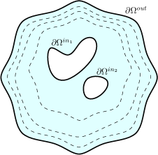
Figure 3: Illustration for smooth stationary $\omega$ where $\Omega:=\text{supp}(\omega)$ is colored in blue, whose boundary is not necessarily connected. The dashed lines are regular level sets of $\omega$, which converges to the outermost boundary. In such case, the stream function is constant on the outermost boundary $\partial\Omega^{out}$, thus Lemma 4.3 implies that the velocity vanishes in the unbounded part of $\Omega^{c}$.

4.3 Nash-Moser theorem

We first prove a bifurcation theorem using the Nash-Moser scheme under some assumptions, which will turn out to be satisfied by our nonlinear functional. We follow the ideas from Berti [7].

Let $2\leq m\in\mathbb{N}$ fixed. We denote

$$X^{k}:=X^{k,m},\quad Y^{k}:=Y^{k,m},\quad C^{\infty}:=C^{\infty}(\mathbb{T}),\quad R:=(R_{1},R_{2},R_{3})\in\left(X^{k+1}\right)^{3}\cap(C^{\infty})^{3},\quad\partial_{\Theta}:=\partial_{\Theta_{3}},$$

for simplicity. Furthermore, for a Banach space $X$ and an element $R\in X$, we denote the norm of $R$ by $|R|_{X}:=\rVert R\rVert_{X}$. In addition, we use the notation $A\lesssim_{a,b}B$ if there exists a constant $C=C(a,b)>0$ depending on some variables $a,b$ such that $A\leq CB$. We also use $c_{0},c_{1},....$ to denote universal constants that may vary from line to line.

Theorem 4.7

Assume that there exists $\Theta_{3}^{*}\in\mathbb{R}$ and an open neighborhood $I\times V^{3}$ of $(\Theta^{*}_{3},0)\in\mathbb{R}\times\left(X^{3}\right)^{3}$ such that for each $2\leq k\in\mathbb{N}$, $G:I\times\left(X^{k+1}\right)^{3}\mapsto\left(Y^{k}\right)^{3}$ satisfies the following: For $(\Theta_{3},R)\in I\times\left(V^{3}\cap(C^{\infty})^{3}\right)$

• (Existence of a curve of trivial solutions) $G(\Theta_{3},0)=0$ for all $\Theta_{3}\in I$.

• (Regularity) It holds that

  $$|G(\Theta_{3},R)|_{(Y^{k})^{3}}\lesssim_{k}1+|R|_{(X^{k+1})^{3}},$$ (4.8)

  $$\left|\partial_{\Theta}G(\Theta_{3},R)\right|_{(Y^{k})^{3}}\lesssim_{k}1+\left|R\right|_{(X^{k+1})^{3}}$$ (4.9)

  $$|D^{2}G(\Theta_{3},R)[h,h]|_{(Y^{k})^{3}}\lesssim_{k}(1+|R|_{(X^{k+3})^{3}})|h|_{(X^{k+1})^{3}}^{2}$$ (4.10)

  $$|\partial_{\Theta}DG(\Theta_{3},R)[h]|_{(Y^{k})^{3}}\lesssim_{k}(1+|R|_{(X^{k+3})^{3}})|h|_{(X^{k+1})^{3}}$$ (4.11)

  $$|\partial_{\Theta}D^{2}G(\Theta^{*}_{3},R)[h,h]|_{(Y^{k})^{3}}\lesssim_{k}(1+|R|_{(X^{k+3})^{3}})|h|_{(X^{k+1})^{3}}^{2}$$ (4.12)

  $$|\partial_{\Theta\Theta}DG(\Theta_{3},R)[h]|_{(Y^{k})^{3}}\lesssim_{k}(1+|R|_{(X^{k+3})^{3}})|h|_{(X^{k+1})^{3}}$$ (4.13)

• (Decomposition of $DG$) $DG(\Theta_{3},R)\in\mathcal{L}((X^{k+1})^{3};(Y^{k})^{3})$ has the following decomposition:

  $$DG(\Theta_{3},R)[h]=a(\Theta_{3},R)[h]+A(\Theta_{3},R)[h],$$

  such that $a(\Theta_{3},R)\in\mathcal{L}((X^{k+1})^{3},(Y^{k})^{3})$, $A(\Theta_{3},R)\in\mathcal{L}((X^{k+1})^{3},Y^{k+1}\times(Y^{k})^{2})$. Also, there exists $0<\eta<1$ such that if $\rVert R\rVert_{(H^{k+2})^{3}}\leq\eta$, then

  $${|a(\Theta_{3},R)[h]|_{(Y^{k})^{3}}\lesssim_{k}|G(\Theta_{3},R)|_{(Y^{k})^{3}}|h|_{(X^{k+1})^{3}}},$$ (4.14)

  $$|A(\Theta_{3},R)[h]|_{Y^{k+1}\times(Y^{k})^{2}}\lesssim_{k}(1+|R|_{(X^{k+3})^{3}})|h|_{(X^{k+1})^{3}},$$ (4.15)

• $A:\mathbb{R}\times(X^{k+3})^{3}\mapsto\mathcal{L}((X^{k+1})^{3},Y^{k+1}\times(Y^{k})^{2})$ is Lipschitz continuous. That is, if

  $$(\Theta_{3}^{1},R^{1}),\ (\Theta_{3}^{2},R^{2})\in I\times(V^{3}\cap(C^{\infty})^{3}),$$

  and $\rVert R^{1}\rVert_{(H^{k+3}(\mathbb{T}))^{2}},\rVert R^{2}\rVert_{(H^{k+3}(\mathbb{T}))^{2}}\leq 1$, it holds that

  $$|A(\Theta_{3}^{1},R^{1})[h]-A(\Theta_{3}^{2},R^{2})|_{(Y^{k})^{3}}\lesssim_{k}\left(|\Theta_{3}^{1}-\Theta_{3}^{2}|+|R^{1}-R^{2}|_{(X^{k+3})^{3}}\right)|h|_{(X^{k+1})^{3}}.$$ (4.16)

• (Tame estimates) There exists $0<\eta<1$ such that if $\rVert R\rVert_{(H^{k+3}(\mathbb{T}))^{3}}\leq\eta$, and $A(\Theta_{3},R)[h]=z$ for some $z\in(C^{\infty})^{3}$ and $h\in\text{Ker}(A(\Theta^{*}_{3},0))^{\perp}$, then $h\in(C^{\infty})^{3}$. Furthermore, for any even $\sigma\in\mathbb{N}\cup\left\{0\right\}$, it holds that

  $$\left|h\right|_{(X^{k+1+\sigma})^{3}}\lesssim_{k,\sigma}(1+\left|R\right|_{(X^{k+4+\sigma})^{3}})\left|z\right|_{Y^{k+1}\times(Y^{k})^{2}}+\left|z\right|_{Y^{k+1+\sigma}\times(Y^{k+\sigma})^{2}}.$$ (4.17)

• (Fredholm index zero) There exist non-zero vectors $v$ and $w$ such that $v$ and $w$ are supported on the $m$-th Fourier mode and

  $$\text{Ker}(A(\Theta_{3}^{*},0))=\text{span}\left\{v\right\},\quad\text{Im}(A(\Theta_{3}^{*},0))^{\perp}=\text{span}\left\{w\right\},$$

• (Transversality) $\partial_{\Theta}A(\Theta_{3}^{*},0)[v]\notin\text{Im}(A(\Theta_{3}^{*},0))$.

Then, for any $k_{0}\geq 2$, there exist a constant $s_{0}=s_{0}(k_{0})>0$ and a curve $[0,s_{0})\ni s\mapsto(\Theta_{3}(s),R(s))\in I\times(X^{k_{0}+1})^{3}$ such that $G(\Theta_{3},R)=0$ and $R(s)\neq 0$ for $s>0$. The curve emanates from $(\Theta_{3}(0),R(0))=(\Theta^{*}_{3},0)$.

Remark 4.8

Note that the evenness of $\sigma$ for the tame estimate in $(\tilde{c}-2)$ is simply because $X^{k}$ is a space of even functions and any odd order derivatives of $h\in X^{k}$ are even.

The rest of this section is devoted to prove Theorem 4.7.

Towards the proof, let $k_{0}\geq 2$ be fixed. We define the projections $P:(X^{k_{0}+1})^{3}\mapsto\text{Ker}(A(\Theta_{3}^{*},0))$ and $Q:(Y^{k_{0}})^{3}\mapsto\text{Im}(A(\Theta_{3}^{*},0))^{\perp}$ by

$$PR:=\left(v\cdot R\right)v\quad\text{ and }\quad QR:=(w\cdot R)w,$$ (4.18)

where $(f\cdot g)$ denotes the usual $L^{2}$ inner product. Note that from the assumptions $(d)$ and $(e)$, we make an ansatz that for sufficiently small $s>0$, the bifurcation curve $s\mapsto(\Theta_{3}(s),R(s))$ can be written as

$$(\Theta_{3}(s),R(s))=\left(\Theta^{*}_{3}+v\cdot\tilde{R}(s),sv+(I-P)\tilde{R}(s)\right),$$

for some $\tilde{R}(s)\in(X^{k_{0}+1})^{3}$ such that $|(I-P)\tilde{R}|_{(X^{k_{0}+1})^{3}}=o(s)$. From this ansatz, we define a family of functionals $\tilde{G_{s}}:(X^{k_{0}+1})^{3}\mapsto(Y^{k_{0}})^{3}$ by

$$\tilde{G}_{s}(R):=G(\Theta^{*}_{3}+v\cdot R,sv+(I-P)R),$$ (4.19)

and look for $R\in(X^{k_{0}+1})^{3}$ such that $\tilde{G}_{s}(R)=0$ and $|(I-P)R|_{(X^{k_{0}+1})^{3}}=o(s)$ for sufficiently small $s>0$. This will be achieved by Newton’s method, where the first approximate solution is $R=0$. To perform Newton’s method, we need to study the linearized operator $D\tilde{G}_{s}$ at each approximate solution $R\neq 0$: For $h\in(X^{k_{0}+1})^{3}$, which can be directly computed from (4.19),

$$D\tilde{G}_{s}(R)[h] :=D_{R}\tilde{G}_{s}(R)[h]$$

$$=\partial_{\Theta}G(\Theta_{3}^{*}+v\cdot R,sv+(I-P)R)(v\cdot h)+DG(\Theta_{3}^{*}+v\cdot R,sv+(I-P)R)[(I-P)h]$$

$$=:T_{s}(R)[h]+a(\Theta_{3}^{*}+v\cdot R,sv+(I-P)R)[(I-P)h],$$ (4.20)

where

$$T_{s}(R)[h]:=\partial_{\Theta}G(\Theta_{3}^{*}+v\cdot R,sv+(I-P)R)(v\cdot h)+A(\Theta_{3}^{*}+v\cdot R,sv+(I-P)R)[(I-P)h].$$ (4.21)

The above decomposition of $D\tilde{G}_{s}$ into $T_{s}+a$ follows from the assumption $(c)$. Recall that Newton’s method relies on the “invertibility” of $T_{s}(R)$ for small $s>0$. However, as we will see in the next lemma, $T_{s}$ is not fully invertible between $(X^{k_{0}+1})^{3}$ and $(Y^{k_{0}})^{3}$, because of its loss of derivatives. This is a motivation of adapting a Nash-Moser scheme in our proof. However, (4.14) suggests that the inverse of $T_{s}$ is a good approximate right inverse of $D\tilde{G}_{s}$. In the next subsection, we will focus on the properties of $T_{s}(R)$.

4.3.1 Analysis of ${T}_{s}$

We will look for a solution $R$ to $\tilde{G}_{s}(R)=0$ in $(X^{k_{0}+1})^{3}$ for small $s>0$. In each step of Newton’s method (Nash-Moser iteration), we will regularize the approximate solution $R_{n}$ (see (4.58)). The theorem will be achieved by proving that $R_{n}$ converges in $(X^{k_{0}+1})^{3}$. However, we will also obtain boundedness of the sequence $R_{n}$ in the higher norms, which is necessary because of the extra regularity conditions as in (c), $(\tilde{c}-1)$ and $(\tilde{c}-2)$. For this reason, we will establish several lemmas assuming that an approximate solution $R$ is more regular then $(X^{k_{0}+1})^{3}$, which will turn out to be true at the end of the proof.

Lemma 4.9

Let $0<\epsilon<1$ and $2\leq k_{0}\in\mathbb{N}$ be fixed. There exist positive constants $s_{0}(\epsilon,k_{0}),\ c_{0}(\epsilon,k_{0})$ and $0<\delta(\epsilon,k_{0})<1$ such that for each $0<s<s_{0}$, the following holds: If

$$|PR|_{(X^{k_{0}+2})^{3}}\leq s^{\epsilon},$$ (4.22)

$$|(I-P)R|_{(X^{k_{0}+2})^{3}}\leq s^{1+\epsilon},$$ (4.23)

$$|R|_{(H^{k_{0}+4})^{3}}\leq\delta,$$ (4.24)

then

• For all $t\in[0,1]$,

  $$(\Theta^{*}_{3}+v\cdot R,sv+(I-P)R)\in I\times V^{3},$$ (4.25)

  where $V^{3}$ is as in Theorem 4.7. Therefore,

  $$T_{s}(R)[h]:=\partial_{\Theta}G(\Theta_{3}^{*}+v\cdot R,sv+(I-P)R)(v\cdot h)+A(\Theta_{3}^{*}+v\cdot R,sv+(I-P)R)[(I-P)h],$$

  is well-defined.

• $T_{s}(R):(X^{k_{0}+1})^{3}\mapsto Y^{k_{0}+1}\times(Y^{k_{0}})^{2}$ is an isomorphism and

  $$|T_{s}(R)[h]|_{Y^{k_{0}+1}\times(Y^{k_{0}})^{2}}\leq c_{0}|h|_{(X^{k_{0}+1})^{3}},$$ (4.26)

  $$|T_{s}(R)^{-1}[z]|_{(X^{k_{0}+1})^{3}}\leq\frac{c_{0}}{s}|z|_{Y^{k_{0}+1}\times(Y^{k_{0}})^{2}},$$ (4.27)

  $$\left|\left(D\tilde{G}_{s}(R)\circ T_{s}(R)^{-1}-I\right)[z]\right|_{(Y^{k_{0}})^{3}}\leq c_{0}|\tilde{G}_{s}(R)|_{(Y^{k_{0}})^{3}}|T_{s}(R)^{-1}[z]|_{(X^{k_{0}+1})^{3}},$$ (4.28)

  for some $c_{0}=c_{0}(\epsilon,k_{0})>0$.

  If $R\in C^{\infty}$, then for any even $\sigma\in\mathbb{N}\cup\left\{0\right\}$ and $z\in X^{k_{0}+1+\sigma}\times(X^{k_{0}+\sigma})^{2}$, we have $T_{s}(R)^{-1}[z]\in\left(X^{k_{0}+1+\sigma}\right)^{3}$. Also, we have that

  $$\left|T_{s}(R)^{-1}[z]\right|_{\left(X^{k_{0}+1+\sigma}\right)^{3}}\leq\frac{c_{0}}{s}\left((1+|R|_{(X^{k_{0}+4+\sigma})^{3}})|z|_{Y^{k_{0}+1}\times(Y^{k_{0}})^{2}}+|z|_{Y^{k_{0}+1+\sigma}\times(Y^{k_{0}+\sigma})^{2}}\right),$$ (4.29)

  where $c_{0}$ may depend on not only $\epsilon,k_{0}$ but also $\sigma$.

• Furthermore, we can choose $c_{0}$ so that when $R=0$, the following hold:

  $$|P(T_{s}(0)^{-1}[z])|_{(X^{k_{0}+1})^{3}}\leq\frac{c_{0}}{s}|z|_{Y^{k_{0}+1}\times(Y^{k_{0}})^{2}},$$ (4.30)

  $$|(I-P)(T_{s}(0)^{-1}[z])|_{(X^{k_{0}+1})^{3}}\leq c_{0}|z|_{Y^{k_{0}+1}\times(Y^{k_{0}})^{2}}.$$ (4.31)

We will frequently use

$$|T_{s}(R)^{-1}z|_{\left(X^{k_{0}+1}\right)^{3}}\leq\frac{c_{0}}{s}|z|_{(Y^{k_{0}+1})^{3}},$$ (4.32)

which is more crude than (4.27).

Proof.

Let us fix $\epsilon>0$ and $k_{0}\geq 2$. We will show that if (4.22)-(4.24) hold for sufficiently small $s>0$ and for some small $\delta>0$ depending on $\epsilon$, then (A),(B) and (C) hold for some $c_{0}>0$.

Proof of (A). To see (A), notice that (4.25) is trivial. From the assumptions (b) and (c) in Theorem 4.7, the linear operator $T_{s}(R)$ is well-defined.

Proof of (B). The estimate (4.26), follows from (4.21), (4.15), (4.9) and

$$|sv+(I-P)R|_{\left(H^{k_{0}+3}\right)^{3}}\lesssim 1+\delta\lesssim 1,$$

where the last inequality follows from (4.24). Before proving (4.27), we first prove that

$$|Q\partial_{\Theta}G(\Theta_{3}^{*}+v\cdot R,sv+(I-P)R)|_{X^{k_{0}+1}\times(X^{k_{0}})^{2}}\geq cs,$$ (4.33)

for some $c=c(\epsilon)>0$. The above inequality is a consequence of the transversality condition $(e)$ in Theorem 4.7. In what follows, $c,c_{1},c_{2},\ldots$ denote positive constants that may change from line to line and depend only on $\epsilon$ but not on $s$.

By the regularity assumptions of $G$ in (b) in Theorem 4.7, we estimate the quantity in (4.33) using a Taylor expansion up to linear order: For a fixed $R$, we set $f(s,y):=Q\partial_{\Theta}G(\Theta_{3}^{*}+v\cdot R,sv+(I-P)y)$, so that

$$f(s,R)=Q\partial_{\Theta}G(\Theta_{3}^{*}+v\cdot R,sv+(I-P)R).$$ (4.34)

Using the fundamental theorem of calculus, we can write

$$f(s,R) :=\int_{0}^{1}\frac{d}{dt}\left(f(s,tR)\right)dt+f(s,0)$$

$$=\int_{0}^{1}\frac{d}{dt}\left(f(s,tR)\right)dt+f(0,0)+\int_{0}^{s}\frac{d}{dt}f(t,0)dt.$$

In terms of $G$, (4.34) and the above equality give us that

$$|Q\partial_{\Theta}G(\Theta_{3}^{*} +v\cdot R,sv+(I-P)R)|_{Y^{k_{0}+1}\times(Y^{k_{0}})^{2}}=|f(s,R)|_{Y^{k_{0}+1}\times(Y^{k_{0}})^{2}}$$

$$\geq-{\sup_{0\leq t\leq 1}\|Q\partial_{\Theta}DG(\Theta_{3}^{*}+v\cdot R,sv+t((I-P)R))\|_{\mathcal{L}((X^{k_{0}+2})^{3},(Y^{k_{0}+1})^{3})}|(I-P)R|_{\left(X^{k_{0}+2}\right)^{3}}}$$

$$\ -{|Q\partial_{\Theta}G(\Theta_{3}^{*}+v\cdot R,0)|_{Y^{k_{0}+1}\times(Y^{k_{0}})^{2}}}$$

$$\ +{\bigg{|}\int_{0}^{s}Q\partial_{\Theta}DG(\Theta_{3}^{*}+v\cdot R,tv)[v]dt\bigg{|}_{Y^{k_{0}+1}\times(Y^{k_{0}})^{2}}}$$

$$=:-L_{1}-L_{2}+L_{3},$$ (4.35)

where the first term after the inequality follows from b) in Theorem 4.7 and

$$\int_{0}^{1}\left|\frac{d}{dt}\left(f(s,tR)\right)\right|_{Y^{k_{0}+1}\times(Y^{k_{0}})^{2}}dt \leq\int_{0}^{1}\left|\frac{d}{dt}\left(f(s,tR)\right)\right|_{(Y^{k_{0}+1})^{3}}dt$$

$$\leq\sup_{0\leq t\leq 1}\left|D_{R}f(s,tR)[R]\right|_{(Y^{k_{0}+1})^{3}},$$

and the rest follows simply from the triangular inequality. Then the regularity assumption (b) in Theorem 4.7 yields that (recall $\rVert R\rVert_{(X^{k_{0}+4})^{3}}<\delta<1$,)

$$L_{1}\leq c_{1}|(I-P)R|_{\left(X^{k_{0}+2}\right)^{3}}\leq c_{1}s^{1+\epsilon},$$ (4.36)

where the last inequality follows from (4.23). For $L_{2}$, we use (a) in Theorem 4.7 to obtain

$$L_{2}=0.$$ (4.37)

To estimate $L_{3}$, we compute

$$L_{3} \geq\bigg{|}\int_{0}^{s}Q\partial_{\Theta}DG(\Theta_{3}^{*},tv)[v]dt\bigg{|}_{Y^{k_{0}+1}\times(Y^{k_{0}})^{2}}-\int_{0}^{s}\sup_{u\in(0,|v\cdot R|)}\bigg{|}Q\partial_{\Theta\Theta}DG(\Theta_{3}^{*}+u,tv)[v]\bigg{|}_{Y^{k_{0}+1}\times(Y^{k_{0}})^{2}}|v\cdot R|dt.$$ (4.38)

For the first integral, we can write

$$Q\partial_{\Theta}DG(\Theta^{*}_{3},tv)[v] =Q\partial_{\Theta}DG(\Theta^{*}_{3},0)[v]+\int_{0}^{t}Q\partial_{\Theta}D^{2}G(\Theta^{*}_{3},uv)[v,v]du$$

$$=QA(\Theta^{*}_{3},0)[v]+\int_{0}^{t}Q\partial_{\Theta}D^{2}G(\Theta^{*}_{3},uv)[v,v]du,$$

where the last equality follows from (a) and (c) in Theorem 4.7, which shows $a(\Theta^{*}_{3},0)=0$. For the integral term, using (4.12), we have

$$\left|Q\partial_{\Theta}D^{2}G(\Theta^{*}_{3},uv)[v,v]\right|_{Y^{k_{0}+1}\times(Y^{k_{0}})^{2}}\lesssim\left|Q\partial_{\Theta}D^{2}G(\Theta^{*}_{3},uv)[v,v]\right|_{(Y^{k_{0}+1})^{3}}\lesssim(1+\rVert R\rVert_{(X^{k_{0}+4})^{3}})\rVert v\rVert_{(X^{k_{0}+2})^{3}}\leq c,$$

where the last inequality follows from (4.24). Therefore

$$\bigg{|}\int_{0}^{s}Q\partial_{\Theta}DG(\Theta_{3}^{*},tv)[v]dt\bigg{|}_{X^{k_{0}+1}\times(X^{k_{0}})^{2}} \geq s\left|QA(\Theta^{*}_{3},0)[v]\right|_{X^{k_{0}+1}\times(X^{k_{0}})^{2}}-\int_{0}^{s}\int_{0}^{t}cdudt$$

$$\geq s\left|Q\partial_{\Theta}DG(\Theta^{*}_{3},0)[v]\right|_{X^{k_{0}+1}\times(X^{k_{0}})^{2}}-c_{2}s^{2}$$

$$\geq c_{3}s-c_{2}s^{2},$$

where the last inequality follows from the transversality (e). For the second integral in (4.38), we have that for sufficiently small $s>0$,

$$\sup_{u\in(0,|v\cdot R|),t\in(0,s)}\left|\partial_{\Theta\Theta}DG(\Theta^{*}_{3}+u,tv)[v]\right|_{Y^{k_{0}+1}\times(Y^{k_{0}})^{2}}\lesssim\sup_{t\in(0,s)}(1+|tv|_{(X^{k_{0}+4})^{3}})|v|_{(X^{k_{0}+2})^{3}}\leq c_{1},$$

for sufficiently small $s$, which follows from (4.13). Hence using (4.22), we obtain from (4.38) that

$$L_{3}\geq c_{3}s-c_{2}s^{2}-c_{1}s^{1+\epsilon}$$ (4.39)

Thus the claim (4.33) follows from (4.3.1) (4.36), (4.37) and (4.39) for small $s$, depending on $\epsilon$.

Towards the proof of (4.27), we will consider how to invert $A(\Theta_{3}^{*}+v\cdot R,sv+(I-P)R)[(I-P)]$. Since the dimension of $\text{Im}(DG(\Theta_{3}^{*},0)^{\perp})$ is one and $w$ is the basis of $\text{Im}(DG(\Theta_{3}^{*},0))^{\perp}$, the above claim (4.33) proves that

$$\left|w\cdot\partial_{\Theta}G(\Theta_{3}^{*}+v\cdot R,sv+(I-P)R)\right|>cs.$$ (4.40)

To simplify the notations, we denote

$$\tilde{A}[h]:=A(\Theta_{3}^{*}+v\cdot R,sv+(I-P)R)[(I-P)h],$$ (4.41)

$$\partial_{\Theta}G:=\partial_{\Theta}G(\Theta^{*}+v\cdot R,sv+(I-P)R).$$

We denote by $Q_{1}$ the projection from $Y^{k_{0}+1}\times\left(Y^{k_{0}}\right)^{2}$ into $\text{Im}(\tilde{A})^{\perp}$. Since the norm of $R$ is small, we expect that the functional structure of $\tilde{A}$ should be similar to the structure of $A(\Theta^{*}_{3},0)$. Indeed, by continuity hypotheses (4.16), (4.24) and Lemma A.15, where we can think of $\tilde{A}$ as a linear map from $\text{Ker}(A(\Theta^{*}_{3},0))$, we can choose $\delta$ small enough so that if (4.24) holds, then there exists $0\neq w_{1}\in Y^{k_{0}+1}\times(Y^{k_{0}})^{2}$ such that

$$\text{Im}(\tilde{A})^{\perp}=\text{span}\left\{w_{1}\right\}$$ (4.42)

$$|w-w_{1}|_{Y^{k_{0}+1}\times(Y^{k_{0}})^{2}}\leq c\delta,$$ (4.43)

$$|\tilde{A}|_{\mathcal{L}(\text{Ker}\left(A(\Theta_{3}^{*},0)\right)^{\perp},\text{Im}(\tilde{A}))}\leq c,$$ (4.44)

$$|\tilde{A}^{-1}|_{\mathcal{L}(\text{Im}(\tilde{A}),\text{Ker}\left(A(\Theta_{3}^{*},0)\right)^{\perp})}\leq c.$$ (4.45)

Now, we claim that we can further restrict $\delta$ if necessary so that

$$\left|w_{1}\cdot\partial_{\Theta}G\right|>cs.$$ (4.46)

In fact, note that (4.22)-(4.23) imply that $R\in(X^{k_{0}+2})^{3}$, thus by (4.9), we have $\partial_{\Theta}G\in(Y^{k_{0}+1})^{3}\subset Y^{k_{0}+1}\times(Y^{k_{0}})^{2}$. Also we have

$$\partial_{\Theta}G =\int_{0}^{1}\partial_{t}\left(\partial_{\Theta}G(\Theta^{*}_{3}+v\cdot R,t(sv+(I-P)R))\right)dt$$

$$=\int_{0}^{1}\partial_{\Theta}DG(\Theta^{*}_{3}+v\cdot R,t(sv+(I-P)R))[sv+(I-P)R]dt,$$

thus

$$\left|\partial_{\Theta}G\right|_{Y^{k_{0}+1}\times(Y^{k_{0}})^{2}}\leq\left|\partial_{\Theta}G\right|_{(Y^{k_{0}+1})^{3}}\leq c|sv+(I-P)R|_{(X^{k_{0}+2})^{2}}\leq cs,$$ (4.47)

where the second inequality follows from (4.9) and the last inequality follows from (4.23). Then it follows that (recall that $f\cdot g$ is the dot product in $L^{2}$ space),

$$|\partial_{\Theta}G\cdot w_{1}| \geq|\partial_{\Theta}G\cdot w|-|\partial_{\Theta}G\cdot(w_{1}-w)|$$

$$\geq c_{1}s-|\partial_{\Theta}G\cdot(w_{1}-w)|$$

$$\geq c_{1}s-cs|w-w_{1}|_{X^{k_{0}+1}\times(X^{k_{0}})^{2}}$$

$$\geq c_{1}s-c\delta s,$$

where we used (4.40), (4.47) and (4.43) for the second, third and the fourth inequality, respectively. Hence, assuming $\delta$ is small, we have (4.46).

To prove (4.27), pick an arbitrary $z\in Y^{k_{0}+1}\times(Y^{k_{0}})^{2}$. There exists a unique $\eta\in\text{Ker}\left(A(\Theta_{3}^{*},0)\right)$ and a unique $h\in\text{Ker}\left(A(\Theta_{3}^{*},0)\right)^{\perp}$ such that

$$(v\cdot\eta)Q_{1}\partial_{\Theta}G=Q_{1}z$$ (4.48)

$$(v\cdot\eta)(I-Q_{1})\partial_{\Theta}G+\tilde{A}[h]=(I-Q_{1})z.$$ (4.49)

In fact, there exists a unique $\eta$ in (4.48) thanks to (4.46) and that $Q_{1}$ is the projection to a one-dimensional space spanned by $w_{1}$. Once $\eta$ is fixed, the existence and the uniqueness of $h$ in (4.49) follows from (4.45). Once $\eta$ and $h$ are determined, it is clear that

$$T_{s}(R)[h+\eta]=(v\cdot(h+\eta))\partial_{\Theta}G+\tilde{A}[\eta+h]=(v\cdot\eta)\partial_{\Theta}G+\tilde{A}[h]=z,$$ (4.50)

where we used $v\cdot h=0$ and $\tilde{A}[\eta]=\tilde{A}[(I-P)\eta]=0$, which follows from the definition of $\tilde{A}$ in (4.41). Therefore $T(R)^{-1}z=h+\eta$. Furthermore we have from (4.48) and (4.49) that

$$|\eta|_{(X^{k_{0}+1})^{3}}\leq c\frac{|z\cdot w_{1}|}{|\partial_{\Theta}G\cdot w_{1}|}$$ (4.51)

$$|h|_{(X^{k_{0}+1})^{3}}\leq|\tilde{A}^{-1}(I-Q_{1})\partial_{\Theta}G(v\cdot\eta)|_{{(X^{k_{0}+1})^{3}}}+|\tilde{A}^{-1}(I-Q_{1})z|_{(X^{k_{0}+1})^{3}}.$$ (4.52)

Using (4.46) and (4.45), we obtain

$$|\eta|_{(X^{k_{0}+1})^{3}}\leq c\frac{|z|_{Y^{k_{0}+1}\times(Y^{k_{0}})^{2}}}{s},$$ (4.53)

$$|h|_{(X^{k_{0}+1})^{3}}\leq c|\partial_{\Theta}G|_{Y^{k_{0}+1}\times(Y^{k_{0}})^{2}}\frac{|z|_{Y^{k_{0}+1}\times(Y^{k_{0}})^{2}}}{s}+c|z|_{Y^{k_{0}+1}\times(Y^{k_{0}})^{2}}\leq c\frac{|z|_{Y^{k_{0}+1}\times(Y^{k_{0}})^{2}}}{s},$$ (4.54)

where we used (4.47). This proves (4.27).

To show (4.28), we compute

$$\left(D\tilde{G}_{s}(R)\circ T_{s}(R)^{-1}-I\right)[z]=a(\Theta_{3}^{*}+v\cdot R,sv+(I-P)R)\circ T(R)^{-1}[z],$$

which follows from (4.20). This implies

$$|\left(D\tilde{G}_{s}(R)\circ T_{s}(R)^{-1}-I\right)[z]|_{\left(X^{k_{0}}\right)^{3}} \leq c|a(\Theta_{3}^{*}-v\cdot R,sv+(I-P)R)\circ T(R)^{-1}[z]|_{\left(X^{k_{0}}\right)^{3}}$$

$$\leq c|G(\Theta_{3}^{*}+v\cdot R,sv+(I-P)R)|_{\left(Y^{k_{0}}\right)^{3}}|T_{s}(R)^{-1}[z]|_{\left(X^{k_{0}+1}\right)^{3}}$$

$$\leq c|\tilde{G}_{s}(R)|_{\left(Y^{k_{0}}\right)^{3}}|T_{s}(R)^{-1}[z]|_{\left(X^{k_{0}+1}\right)^{3}},$$

where we used (4.14) to get the second inequality and used the definition of $\tilde{G}_{s}(R)$ to obtain the last inequality.

In order to prove (4.29), we improve on the estimates in (4.51) and (4.52). For (4.51), recall that $\eta$ is in a one-dimensional space, span$\left\{v\right\}$ and $v$ is supported on the $m$-th Fourier mode. Thus,

$$|\eta|_{(X^{k_{0}+1+\sigma})^{3}}\leq c|\eta|_{(X^{k_{0}+1})^{3}}\leq c\frac{|z|_{Y^{k_{0}+1}\times(Y^{k_{0}})^{2}}}{s},$$ (4.55)

where $c$ may depend on $\sigma$. Furthermore, $(\tilde{c}$-2) in Theorem 4.7 and (4.49) give us that

$$|h|_{(X^{k_{0}+1+\sigma})^{3}} \leq c(1+\left|R\right|_{(X^{k_{0}+4+\sigma})^{3}})\left(\left|(v\cdot\eta)\partial_{\Theta}G\right|_{Y^{k_{0}+1}\times(Y^{k_{0}})^{2}}+\left|z\right|_{Y^{k_{0}+1}\times(Y^{k_{0}})^{2}}\right)$$

$$\ +c\left(\left|(v\cdot\eta)\partial_{\Theta}G\right|_{Y^{k_{0}+1+\sigma}\times(Y^{k_{0}+\sigma})^{2}}+\left|z\right|_{Y^{k_{0}+1+\sigma}\times(Y^{k_{0}+\sigma})^{2}}\right).$$ (4.56)

Using (4.47) and (4.53), we have

$$\left|(v\cdot\eta)\partial_{\Theta}G\right|_{Y^{k_{0}+1}\times(Y^{k_{0}})^{2}}\leq\left|\partial_{\Theta}G\right|_{{Y^{k_{0}+1}\times(Y^{k_{0}})^{2}}}|v\cdot\eta|\leq c\left|z\right|_{Y^{k_{0}+1}\times(Y^{k_{0}})^{2}}.$$

For the higher norm of $\partial_{\Theta}G$, we use (4.9) and and (4.53) and obtain

$$\left|(v\cdot\eta)\partial_{\Theta}G\right|_{Y^{k_{0}+1+\sigma}\times(Y^{k_{0}+\sigma})^{2}} \leq c\left|\partial_{\Theta}G\right|_{(Y^{k_{0}+1+\sigma})^{3}}|v\cdot\eta|$$

$$\leq\frac{c}{s}\left(1+\left|R\right|_{(X^{k_{0}+2+\sigma})^{3}}\right)\left|z\right|_{Y^{k_{0}+1}\times(Y^{k_{0}})^{2}}.$$

Therefore, (4.56) gives us

$$|h|_{(X^{k_{0}+1+\sigma})^{3}}\leq\frac{c}{s}\left((1+\left|R\right|_{(X^{k_{0}+4+\sigma})^{3}})\left|z\right|_{Y^{k_{0}+1}\times(Y^{k_{0}})^{2}}+\left|z\right|_{Y^{k_{0}+1+\sigma}\times(Y^{k_{0}+\sigma})^{2}}\right).$$

Combining with (4.55), we obtain (4.29).

Proof of (C). Finally, if $R=0$, then we have $|\partial_{\Theta}G|_{Y^{k_{0}+1}\times(Y^{k_{0}})^{2}}=|\partial_{\Theta}G(\Theta_{3},sv)|_{{Y^{k_{0}+1}\times(Y^{k_{0}})^{2}}}\leq cs$. Therefore we can improve (4.54) and obtain

$$|h|_{(X^{k_{0}+1})^{3}}\leq c|z|_{Y^{k_{0}+1}\times(Y^{k_{0}})^{2}},$$

which implies (4.31). (4.27) follows trivially from (4.30). This completes the proof. ∎

Lemma 4.10

Let $\tilde{G}_{s}$ be as in (4.19). Then there exists an open set $V^{3}$ near $0\in(X^{3})^{3}$ such that for all $R,\tilde{R}\in V^{3}$ and $k\geq 2$,

• (Initial value) $|\tilde{G}_{s}(0)|_{(X^{k})^{3}}\lesssim_{k}s^{2}.$

• (Taylor estimate) If $\rVert R\rVert_{(X^{k+3})^{3}},\rVert\tilde{R}\rVert_{(X^{k+3})^{3}}\leq\eta$ for some $0<\eta=\eta(k)<1$, then

  $$\begin{cases}|D\tilde{G}_{s}(R)[h]|_{(Y^{k})^{3}}\lesssim_{k}|h|_{(X^{k+1})^{3}}\\ |\tilde{G}_{s}(\tilde{R})-\tilde{G}_{s}(R)-D\tilde{G}_{s}(R)[\tilde{R}-R]|_{(Y^{k})^{3}}\lesssim_{k}|\tilde{R}-R|_{(X^{k+1})^{3}}^{2}\\ |\tilde{G}_{s}(\tilde{R})-\tilde{G}_{s}(R)-D\tilde{G}_{s}(R)[\tilde{R}-R]-\frac{1}{2}D^{2}\tilde{G}_{s}[\tilde{R}-R,\tilde{R}-R]|_{(Y^{k})^{3}}\lesssim_{k}|\tilde{R}-R|_{(X^{k+1})^{3}}^{3}.\end{cases}$$

Proof.

(a’) follows from the fact that $v\in\text{Ker}(DG(\Theta_{3}^{*},0))$ and $G(\Theta_{3}^{*},0)=0$. (b’) is due to (b) in Theorem 4.7. ∎

4.3.2 Nash-Moser iteration

For $\beta,N>0$ and $2\leq k\in\mathbb{N}$, we consider a regularizing operator $S(N):(X^{k})^{3}\mapsto(C^{\infty})^{3}$ such that

$$\begin{cases}|S(N)R|_{(X^{k+\beta})^{3}}\lesssim_{k,\beta}N^{\beta}|R|_{(X^{k})^{3}}&\forall\ R\in(H^{k})^{3}\\ |(I-S(N))R|_{(H^{k})^{3}}\lesssim_{k,\beta}N^{-\beta}|R|_{(X^{k+\beta})^{3}}&\forall\ R\in(H^{k+\beta})^{3}.\end{cases}$$ (4.57)

Note that we can choose $S$ so that $PS(N)=S(N)P$, since $v$ is supported on the $m$-th Fourier mode (see (d) in Theorem 4.7).

For $N_{n}>1$ and even integer $\beta>0$, which will be chosen later, we set

$$\begin{cases}R_{n+1}=R_{n}-S(N_{n})T_{s}(R_{n})^{-1}[\tilde{G}_{s}(R_{n})]&\text{ for }n\geq 0\\ R_{0}=0,\end{cases}$$ (4.58)

and

$$\begin{cases}a_{n}:=|R_{n+1}-R_{n}|_{(X^{k_{0}+1})^{3}}\\ a^{\prime}_{n}:=|R_{n+1}-R_{n}|_{(X^{k_{0}+2})^{3}}\\ a^{\prime\prime}_{n}=|R_{n+1}-R_{n}|_{(X^{k_{0}+4})^{3}}\\ b_{n}:=|\tilde{G}_{s}(R_{n})|_{(Y^{k_{0}})^{3}}\\ C_{n}:=|T_{s}(R_{n})^{-1}[\tilde{G}_{s}(R_{n})]|_{(X^{k_{0}+1+\beta})^{3}}.\end{cases}$$ (4.59)

Note that our goal is to show that $\sum_{n=0}^{\infty}a_{n}<\infty$, which implies that $R_{n}$ converges in $(X^{k_{0}+1})^{3}$. In order to prove the assumptions in (4.22)-(4.24), we will need the boundedness of $a_{n}^{\prime}$ and $a_{n}^{\prime\prime}$ as well.

Lemma 4.11

Let $\epsilon>0$ and $k_{0}\geq 2$ fixed and let $s_{0}$ and $\delta$ be defined as in Lemma 4.9. We also assume that $\delta$ is even smaller if necessary, so that $\delta<\eta(k_{0})$ where $\eta(k_{0})$ is as in (b’) in Lemma 4.10. For any $n\geq 0$ such that $R_{n}$ satisfies (4.22), (4.23) and (4.24) for some $s\in(0,s_{0})$, then we have

$$a_{0}\lesssim_{\epsilon,k_{0}}s,$$ (4.60)

$$a_{n}\lesssim_{\epsilon,k_{0}}\frac{1}{s}N_{n}b_{n} \text{ for }n\geq 1,$$ (4.61)

$$b_{0}\lesssim_{\epsilon,k_{0},\beta}s^{2}$$ (4.62)

$$b_{1}\lesssim_{\epsilon,k_{0},\beta}(N_{0}^{3}+1)s^{3}+N_{0}^{-\beta}C_{0}.$$ (4.63)

$$b_{n+1}\lesssim_{\epsilon,k_{0},\beta}a_{n}^{2}+\frac{1}{s}N_{n}b_{n}^{2}+N_{n}^{-\beta}(1+b_{n})C_{n} \text{ for }n\geq 1,$$ (4.64)

$$a^{\prime}_{n}\lesssim_{\epsilon,k_{0}}\frac{1}{s}N_{n}^{2}b_{n} \text{ for }n\geq 0,$$ (4.65)

$$a^{\prime\prime}_{n}\lesssim_{\epsilon,k_{0}}\frac{1}{s}N_{n}^{4}b_{n} \text{ for }n\geq 0.$$ (4.66)

Furthermore, we have

$$|PR_{1}|_{(X^{k_{0}+2})^{3}}\lesssim_{\epsilon,k_{0}}N_{0}s$$ (4.67)

$$|(I-P)R_{1}|_{(X^{k_{0}+2})^{3}}\lesssim_{\epsilon,k_{0}}N_{0}s^{2}.$$ (4.68)

Proof.

Proof of (4.60), (4.61), (4.67) and (4.68). We first claim that

$$|PR_{1}|_{(X^{k_{0}+1})^{3}}\lesssim s$$ (4.69)

$$|(I-P)R_{1}|_{(X^{k_{0}+1})^{3}}\lesssim s^{2},$$ (4.70)

Let us prove (4.69) first. Thanks to (a’) in Lemma 4.10 and (4.30), we have

$$|PR_{1}|_{(X^{k_{0}+1})^{3}}=|S(N_{0})PT_{s}(0)^{-1}[\tilde{G}_{s}(0)]|_{(X^{k_{0}+1})^{3}}\lesssim|PT_{s}(0)^{-1}[\tilde{G}_{s}(0)]|_{(X^{k_{0}+1})^{3}}\lesssim\frac{1}{s}|\tilde{G}_{s}(0)|_{(Y^{k_{0}}+1)^{3}}\lesssim s,$$

where we used that $S(N_{0})$ and $P$ commute to obtain the first equality. To prove (4.70), we use (4.31) and compute

$$|(I-P)R_{1}|_{(X^{k_{0}+1})^{3}} \lesssim|S(N_{0})(I-P)T_{s}(0)^{-1}[\tilde{G}_{s}(0)]|_{(X^{k_{0}+1})^{3}}$$

$$\lesssim|(I-P)T_{s}(0)^{-1}[\tilde{G}_{s}(0)]|_{(X^{k_{0}+1})^{3}}$$

$$\lesssim|\tilde{G}_{s}(0)|_{(Y^{k_{0}+1})^{3}}$$

$$\lesssim s^{2},$$

which proves (4.70). With the claim, (4.60) follows immediately. (4.61) (4.67) and (4.68) can be proved in exactly the same way as above using (4.57).

Proof of (4.62), (4.63) and (4.64). Note that Lemma 4.10 immediately implies (4.62). Now, let us prove (4.63) and (4.64). We have

$$b_{n+1}:=|\tilde{G}_{s}(R_{n+1})|_{(Y^{k_{0}})^{3}} \lesssim{|\tilde{G}_{s}(R_{n+1})-\tilde{G}_{s}(R_{n})-D\tilde{G}_{s}(R_{n})[R_{n+1}-R_{n}]|_{(Y^{k_{0}})^{3}}}$$

$$\ +{|\tilde{G}_{s}(R_{n})+D\tilde{G}_{s}(R_{n})[R_{n+1}-R_{n}]|_{(Y^{k_{0}})^{3}}}$$

$$=:J_{1}+J_{2},$$ (4.71)

We claim that

$$\begin{cases}J_{1}\lesssim s^{3}&\text{ if }n=0\\ J_{1}\lesssim a_{n}^{2}=|R_{n+1}-R_{n}|_{(X^{k_{0}+1})^{3}}^{2}&\text{ if }n\geq 1.\end{cases}$$ (4.72)

If $n=0$, we have

$$J_{1} \lesssim\bigg{|}\tilde{G}_{s}({R_{1}})-\tilde{G}_{s}(0)-D\tilde{G}_{s}(0)[R_{1}]-\frac{1}{2}D^{2}\tilde{G}_{s}(0)\left[R_{1},R_{1}\right]\bigg{|}_{(Y^{k_{0}})^{3}}+\frac{1}{2}|D^{2}\tilde{G}_{s}(0)[R_{1},R_{1}]|_{(Y^{k_{0}})^{3}}$$

$$\lesssim|R_{1}|^{3}_{(X^{k_{0}+1})^{3}}+\frac{1}{2}|D^{2}\tilde{G}_{s}(0)[R_{1},R_{1}]|_{(Y^{k_{0}})^{3}}$$

$$\lesssim s^{3}+\frac{1}{2}|D^{2}\tilde{G}_{s}(0)[R_{1},R_{1}]|_{(Y^{k_{0}})^{3}},$$

where we used (b’) in Lemma 4.10 in the second inequality and (4.69) and (4.70) in the last inequality. To estimate $D^{2}\tilde{G}$, we recall the definition of $\tilde{G}_{s}$ and compute

$$D^{2}\tilde{G}_{s}(0)[R_{1},R_{1}] =\left(\frac{d}{dt}\right)^{2}G(\Theta_{3}^{*}+tv\cdot R_{1},sv+(I-P)tR_{1})\bigg{|}_{t=0}$$

$$=\partial_{\Theta\Theta}G(\Theta_{3}^{*},sv)(v\cdot R_{1})^{2}+2(v\cdot R_{1})\partial_{\Theta}DG(\Theta_{3}^{*},sv)[(I-P)[R_{1}]]$$

$$\ +D^{2}G(\Theta_{3}^{*},sv)\left[(I-P)R_{1},(I-P)R_{1}\right].$$

Since $\partial_{\Theta\Theta}G(\Theta_{3}^{*},0)=0$, therefore

$$\left|\partial_{\Theta\Theta}G(\Theta^{*}_{3},sv)\right|_{(Y^{k_{0}})^{3}}=\left|\int_{0}^{s}\frac{d}{dt}\left(\partial_{\Theta\Theta}G(\Theta^{*}_{3},tv)\right)dt\right|_{(Y^{k_{0}})^{3}}\lesssim s,$$

which implies $|\partial_{\Theta\Theta}G(\Theta_{3}^{*},sv)(v\cdot R_{1})^{2}|_{(Y^{k_{0}})^{3}}\lesssim s^{3}$, since $|v\cdot R_{1}|\lesssim|PR_{1}|_{(X^{k_{0}+1})^{3}}\lesssim s$, which follows from (4.69). Also it follows from (b), (4.69) and (4.70) that

$$|2(v\cdot R_{1})\partial_{\Theta}DG(\Theta_{3}^{*},sv)[(I-P)[R_{1}]]|_{(Y^{k_{0}})^{3}}\lesssim s^{3},$$

$$|D^{2}G(\Theta_{3}^{*},sv)[(I-P)R_{1},(I-P)R_{1}]|_{(Y^{k_{0}})^{3}}\lesssim s^{4},$$

therefore, $|D^{2}\tilde{G}_{s}(0)[R_{1},R_{1}]|_{(Y^{k_{0}})^{3}}\lesssim s^{3}$. Thus, we have $J_{1}\lesssim s^{3}$, which proves (4.72) for $n=0$. If $n\geq 1$, the claim in (4.72) follows immediately from (b’) in Lemma 4.10.

In order to estimate $J_{2}$ in (4.3.2), we have that for $n\geq 0$,

$$J_{2} \lesssim{|(I-D\tilde{G}_{s}(R_{n})\circ T_{s}(R_{n})^{-1})[\tilde{G}_{s}(R_{n})]|_{(Y^{k_{0}})^{3}}}$$

$$\ +{|D\tilde{G}_{s}(R_{n})\left(I-S(N_{n})\right)T_{s}(R_{n})^{-1}[\tilde{G}_{s}(R_{n})]|_{(Y^{k_{0}})^{3}}}$$

$$=:J_{21}+J_{22}.$$

Then it follows from (4.57) and (4.28) that

$$J_{21} \lesssim|\tilde{G}_{s}(R_{n})|_{(Y^{k_{0}})^{3}}|T_{s}(R_{n})^{-1}[\tilde{G}_{s}(R_{n})]|_{(X^{k_{0}+1})^{3}}$$

$$\lesssim|\tilde{G}_{s}(R_{n})|_{(Y^{k_{0}})^{3}}|S(N_{n})T_{s}(R_{n})^{-1}[\tilde{G}_{s}(R_{n})]|_{(X^{k_{0}+1})^{3}}$$

$$\ +|\tilde{G}_{s}(R_{n})|_{(Y^{k_{0}})^{3}}|\left(I-S(N_{n})\right)T_{s}(R_{n})^{-1}[\tilde{G}_{s}(R_{n})]|_{(X^{k_{0}+1})^{3}}$$

$$\lesssim N_{n}|\tilde{G}_{s}(R_{n})|_{(Y^{k_{0}})^{3}}|T_{s}(R_{n})^{-1}[\tilde{G}_{s}(R_{n})]|_{(X^{k_{0}})^{3}}$$

$$\ +N_{n}^{-\beta}|\tilde{G}_{s}(R_{n})|_{(Y^{k_{0}})^{3}}|T_{s}(R_{n})^{-1}[\tilde{G}_{s}(R_{n})]|_{(X^{k_{0}+1+\beta})^{3}}$$

$$\lesssim\frac{1}{s}N_{n}|\tilde{G}_{s}(R_{n})|_{(Y^{k_{0}})^{3}}^{2}+N_{n}^{-\beta}|\tilde{G}_{s}(R_{n})|_{(Y^{k_{0}})^{3}}|T_{s}(R_{n})^{-1}[\tilde{G}_{s}(R_{n})]|_{(X^{k_{0}+1+\beta})^{3}}$$

$$\lesssim\frac{1}{s}N_{n}b_{n}^{2}+N_{n}^{-\beta}b_{n}C_{n},$$

where the fourth inequality follows from (4.32). Also we have

$$J_{22}\lesssim|\left(I-S(N_{n})\right)T_{s}(R_{n})^{-1}[\tilde{G}_{s}(R_{n})]|_{(X^{k_{0}+1})^{3}}\lesssim N_{n}^{-\beta}C_{n}.$$

Hence we have for $n\geq 0$ that

$$J_{2}\lesssim\frac{1}{s}N_{n}b_{n}^{2}+N_{n}^{-\beta}(1+b_{n})C_{n}.$$ (4.73)

Thus with (4.3.2), (4.72), (4.73) and (a’) in lemma 4.10, we have that

$$\begin{cases}b_{1}\lesssim(1+N_{0})s^{3}+N_{0}^{-\beta}C_{0}\\ b_{n+1}\lesssim a_{n}^{2}+\frac{1}{s}N_{n}b_{n}^{2}+N_{n}^{-\beta}(1+b_{n})C_{n}&\text{ for }n\geq 1.\end{cases}$$ (4.74)

Proof of (4.65) and (4.66). Finally, for (4.65) and (4.66), we use (4.32) to compute

$$|R_{n+1}-R_{n}|_{(X^{k_{0}+2})^{3}}=|S(N_{n})T_{s}(R_{n})^{-1}[\tilde{G}_{s}(R_{n})]|_{\left(X^{k_{0}+2}\right)^{3}}\lesssim N_{n}^{2}\frac{1}{s}b_{n},$$ (4.75)

$$|R_{n+1}-R_{n}|_{(X^{k_{0}+4})^{3}}=|S(N_{n})T_{s}(R_{n})^{-1}[\tilde{G}_{s}(R_{n})]|_{\left(X^{k_{0}+4}\right)^{3}}\lesssim N_{n}^{4}\frac{1}{s}b_{n}.$$ (4.76)

This finishes the proof. ∎

Let us now derive a recursive formula for $C_{n}$.

Lemma 4.12

For $j=0,\ldots,n-1$ assume that $R_{j}$ satisfies the same assumptions as in Lemma 4.11, that is, given $\epsilon>0$ and $k_{0}\geq 2$, $R_{j}$ satisfies (4.22), (4.23) and (4.24) and the assumptions of Lemma 4.10 for $s\in(0,s_{0}(\epsilon,k_{0}))$ and $\delta=\delta(\epsilon,k_{0})>0$. Then,

$$C_{n}\lesssim_{\epsilon,k_{0},\beta}\frac{1}{s}\left(1+n\sup_{j=0,\ldots n-1}N_{j}^{4}C_{j}\right),\quad\text{ for $n\geq 1$ and }\quad C_{0}\lesssim_{\epsilon,k_{0},\beta}s.$$

Proof.

It follows from (a’) in Lemma 4.10 and (4.29) in Lemma 4.9 that

$$C_{0}\lesssim\frac{1}{s}|\tilde{G}_{s}(0)|_{Y^{k_{0}+1+\beta}\times(Y^{k_{0}+\beta})^{2}}\lesssim\frac{1}{s}|\tilde{G}_{s}(0)|_{(Y^{k_{0}+1+\beta})^{3}}\lesssim s.$$

Now let us assume that $n\geq 1$. It follows from the definition of $C_{n}$ in (4.59) and (4.29) that (recall that $\beta$ is even)

$$C_{n}\lesssim\frac{1}{s}\left((1+|R_{n}|_{(X^{k_{0}+4+\beta})^{3}})|\tilde{G}_{s}(R_{n})|_{Y^{k_{0}+1}\times(Y^{k_{0}})^{2}}+|\tilde{G}_{s}(R_{n})|_{Y^{k_{0}+1+\beta}\times(Y^{k_{0}+\beta})^{2}}\right).$$

Using (4.8), we have

$$|\tilde{G}_{s}(R_{n})|_{Y^{k_{0}+1}\times(Y^{k_{0}})^{2}}\lesssim|\tilde{G}_{s}(R_{n})|_{(Y^{k_{0}+1})^{3}}\lesssim 1+|R_{n}|_{(X^{k_{0}+2})^{3}}\lesssim 1,$$

$$|\tilde{G}_{s}(R_{n})|_{Y^{k_{0}+1+\beta}\times(Y^{k_{0}+\beta})^{2}}\lesssim 1+|R_{n}|_{(X^{k_{0}+2+\beta})^{3}}.$$

therefore, we have

$$C_{n}\lesssim\frac{1}{s}(1+|R_{n}|_{(X^{k_{0}+4+\beta})^{3}}).$$

For $R_{n}$, we have

$$|R_{n}|_{(X^{k_{0}+4+\beta})^{3}} \lesssim\sum_{j=0}^{n-1}\left|R_{j+1}-R_{j}\right|_{(X^{k_{0}+4+\beta})^{3}}$$

$$\lesssim\sum_{j=0}^{n-1}\left|S(N_{j})T_{s}(R_{j})^{-1}[\tilde{G}_{s}(R_{j})]\right|_{(X^{k_{0}+4+\beta})^{3}}$$

$$\lesssim\sum_{j=0}^{n-1}N_{j}^{3}C_{j}$$

$$\lesssim n\sup_{j=0,\ldots,n-1}N_{j}^{3}C_{j}.$$

Hence, we obtain the desired result. ∎

Now we are ready to prove the main theorem of this section.

• Proof of Theorem 4.7: We fix $k_{0}\geq 2$ and pick $\tilde{\epsilon},\ \tilde{s}>0$ so that

  $$\sum_{k=1}^{\infty}s^{-1+2\left(\frac{67}{64}\right)^{k}}\leq s^{1+\tilde{\epsilon}}\text{ for all $s\in(0,\tilde{s})$.}$$ (4.77)

  And we choose

  $$\ \beta:=816\quad\text{ and }\quad\epsilon:=\min\left\{\frac{1}{4},\frac{\tilde{\epsilon}}{2}\right\}>0,$$ (4.78)

  and let $s_{0}=s_{0}(\epsilon,k_{0}),$ $\delta=\delta(\epsilon,k_{0})$ be as in Lemma 4.9. As before, we can also assume $\delta$ is small enough so that $\delta<\eta(k_{0})$ where $\eta$ is as in (b’) in Lemma 4.10. Since $k_{0}$, $\epsilon$ and $\beta$ are fixed, by Lemma 4.11 and 4.12, we can find a constant $K>0$ such that as long as $R_{n}$ satisfies (4.22),(4.23) and (4.24), for some $s\in(0,s_{0})$, it holds that for any sequence of positive numbers $N_{n}$, and

  $$a_{0}\leq Ks$$ (4.79)

  $$|PR_{1}|_{(X^{k_{0}+2})^{3}}\leq KN_{0}s$$ (4.80)

  $$|(I-P)R_{1}|_{(X^{k_{0}+2})^{3}}\leq KN_{0}s^{2}.$$ (4.81)

  $$a_{n}\leq\frac{K}{s}N_{n}b_{n}\quad\text{for $n\geq 1$,}$$ (4.82)

  $$b_{0}\leq Ks^{2},$$ (4.83)

  $$b_{1}\leq K\left((N_{0}^{3}+1)s^{3}+N_{0}^{-\beta}C_{0}\right)$$ (4.84)

  $$b_{n+1}\leq K(a_{n}^{2}+\frac{1}{s}N_{n}b_{n}^{2}+N_{n}^{-\beta}(1+b_{n})C_{n})\quad\text{ for $n\geq 1$},$$ (4.85)

  $$a^{\prime}_{n}\leq\frac{K}{s}N_{n}^{2}b_{n}\quad\text{ for $n\geq 0$},$$ (4.86)

  $$a^{\prime\prime}_{n}\leq\frac{K}{s}N_{n}^{4}b_{n}\quad\text{ for $n\geq 0$},$$ (4.87)

  $$C_{n}\leq\frac{K}{s}\left(1+n\sup_{j=0,\ldots n-1}\left|N_{j}^{4}C_{j}\right|\right)\quad\text{ for $n\geq 1$,}$$ (4.88)

  $$C_{0}\leq Ks.$$ (4.89)

  In what follows, we assume without loss of generality that

  $$K>1,\quad\text{ and }\quad\delta<1.$$ (4.90)

  For such $K$, we can find $s^{*}$ such that for all $s\in(0,s^{*})$ (each of them can be easily verified for small enough $s>0$),

  $$2Kn<s^{-2\left(\frac{67}{64}\right)^{n-1}+1}\quad\text{ for all $n\geq 1$},$$ (4.91)

  $$4K^{3}s^{\frac{7}{16}}<\frac{1}{2},$$ (4.92)

  $$Ks^{\frac{\tilde{\epsilon}}{2}}\leq\frac{1}{2},$$ (4.93)

  $$s<1,$$ (4.94)

  $$K^{2}s^{\frac{3}{4}}\leq\frac{1}{2}\delta,$$ (4.95)

  $$K\sum_{k=1}^{\infty}s^{-1+\frac{127}{64}\left(\frac{67}{64}\right)^{k}}\leq\frac{1}{2}\delta,$$ (4.96)

  $$K(n+2)\leq s^{1-2\left(\frac{67}{64}\right)^{n}}\text{ for all $n\geq 0$},$$ (4.97)

  $$3K^{3}\leq s^{2+\left(-\frac{139}{32}+\frac{143}{64}\cdot\frac{67}{64}\right)\left(\frac{67}{64}\right)^{n}}\text{ for all $n\geq 1$},$$ (4.98)

  $$3K\leq s^{1+\left(-\frac{141}{32}+\frac{143}{64}\left(\frac{67}{64}\right)\right)\left(\frac{67}{64}\right)^{n}}\text{ for all $n\geq 1$},$$ (4.99)

  $$6K\leq s^{\left(-\frac{816}{16}+\frac{768}{16}+\frac{143}{64}\frac{67}{64}\right)\left(\frac{67}{64}\right)^{n}}\text{ for all $n\geq 1$}.$$ (4.100)

  Lastly, we fix $s\in(0,\min\left\{s_{0},s^{*},\tilde{s}\right\})$ and

  $$N_{n}:=s^{-\frac{1}{16}\left(\frac{67}{64}\right)^{n}}\quad\text{ for $n\geq 0$.}$$ (4.101)

  We claim that for all $n\geq 0$,

  • : $R_{n+1}$ satisfies (4.22),(4.23) and (4.24).

  • : $C_{n}\leq N_{n}^{768}$.

  • : $b_{n+1}\leq s^{\frac{143}{64}\left(\frac{67}{64}\right)^{n+1}}$.

  • : $a_{n+1}\leq Ks^{-1+\frac{139}{64}\left(\frac{67}{64}\right)^{n+1}}$.

  Once we have the above claims, then $(P1)_{n}$ justifies all the recurrence formulae above for all $n\in\mathbb{N}$, which follows from Lemma 4.11 and 4.12. Also, it is clear from (4.82) and $(P4)_{n}$ that

  $$\sum_{n=0}^{\infty}a_{n}\leq KN_{0}s+K\sum_{n=1}^{\infty}s^{-1+\frac{139}{64}\left(\frac{67}{64}\right)^{n}}<\infty.$$

  Therefore $R_{n}$ is a Cauchy sequence in $(X^{k_{0}+1})^{3}$, and we can find a limit $R_{\infty}:=\lim_{n\to\infty}R_{n}$. Then, $(P3)_{n}$ and the continuity of the functional $R\mapsto\tilde{G}_{s}$ implies that $\tilde{G}_{s}(R_{\infty})=0$. From the definition of $\tilde{G}_{s}$ in (4.19), this implies the existence of a solution $R=R(s)\neq 0$ for each $s\in(0,\min\left\{s_{0},s^{*},\tilde{s}\right\})$ and finishes the proof.

  Now we prove the claim $(Pi)_{n}$ for $i=1,\ldots,4$. We will follow the usual induction argument.

  Initial step. In the initial case, we assume that $n=0$. We first prove $(P1)_{0}$. It follows from (4.80),(4.81) and (4.101) that

  $$|PR_{1}|_{(X^{k_{0}+2})^{3}}\leq Ks^{\frac{15}{16}}\leq s^{\frac{1}{4}}\leq s^{\epsilon}$$ (4.102)

  $$|(I-P)R_{1}|_{(X^{k_{0}+2})^{3}}\leq Ks^{1+\frac{15}{16}}\leq s^{1+\frac{1}{4}}\leq s^{1+\epsilon},$$ (4.103)

  where the two second inequalities follow from (4.92) ($Ks^{\frac{15}{16}}\leq 4K^{3}s^{\frac{7}{16}}s^{\frac{1}{2}}<s^{\frac{1}{4}}$) and the last inequalities follow from (4.94) and (4.78). Furthermore, it follows from (4.87), (4.83) and (4.101) that

  $$|R_{1}|_{(X^{k_{0}+4})^{3}}=a^{\prime\prime}_{0}\leq\frac{K}{s}\cdot\left(s^{-\frac{1}{16}}\right)^{4}\cdot\left(Ks^{2}\right)\leq K^{2}s^{\frac{3}{4}}\leq\frac{1}{2}\delta,$$ (4.104)

  where the last inequality follows from (4.95). Therefore $(P1)_{0}$ holds for $n=0$. $(P2)_{0}$ follows immediately from (4.89) and (4.101). In order to prove $(P3)_{0}$, note that thanks to (4.84), it is enough to show that

  $$K\left((N_{0}^{3}+1)s^{3}+N_{0}^{-\beta}C_{0}\right)\leq s^{\frac{143}{64}\cdot\frac{67}{64}},$$

  in other words,

  $$K\left(s^{\frac{45}{16}}+s^{3}+Ks^{\frac{816}{16}}s\right)\leq s^{\frac{143}{64}\cdot\frac{67}{64}},$$

  where we used (4.78), (4.89) and (4.101). By (4.94), $s^{\frac{45}{16}}$ is the largest value among the three in the parentheses, hence it is sufficient to show that $3K^{2}<s^{\frac{143}{64}\cdot\frac{67}{64}-\frac{45}{16}}.$ Since $\frac{143}{64}\cdot\frac{67}{64}-\frac{45}{16}>-\frac{1}{2}$, it is enough to show that $3K^{3}\leq s^{-\frac{1}{2}}$, which follows from (4.92). $(P4)_{0}$ follows from (4.82), (4.101) and $(P3)_{0}$.

  Induction step. In this step, we assume that $(Pi)_{k}$ is true for all $0\leq k\leq n_{0}$ and aim to prove $(Pi)_{n_{0}+1}$. Let us prove $(P1)_{n_{0}+1}$ first. It follows from (4.86), (4.101) and $(P3)_{k}$ for $k=0,\ldots,n_{0}$, that

  $$\sum_{k=1}^{n_{0}+1}a^{\prime}_{k}\leq K\sum_{k=1}^{n_{0}+1}s^{-1}\left(s^{-\frac{1}{16}\left(\frac{67}{64}\right)^{k}}\right)^{2}\cdot s^{\frac{143}{64}\left(\frac{67}{64}\right)^{k}}\leq K\sum_{k=1}^{n_{0}+1}s^{-1+2\left(\frac{67}{64}\right)^{k}}\leq Ks^{1+\tilde{\epsilon}},$$

  where the last inequality follows from our choice on $\tilde{\epsilon}$ and $s\in\tilde{s}$ in (4.77). Hence, we have

  $$\sum_{k=1}^{n_{0}+1}a^{\prime}_{k}\leq\left(Ks^{\frac{\tilde{\epsilon}}{2}}\right)s^{1+\frac{\tilde{\epsilon}}{2}}\leq\frac{1}{2}s^{1+\frac{\tilde{\epsilon}}{2}}\leq\frac{1}{2}s^{1+\epsilon},$$

  where the second inequality follows from (4.93) and the last inequality follows from (4.78) and (4.94). Therefore we obtain

  $$|PR_{n_{0}+2}|_{(X^{k_{0}+2})^{3}}\leq|PR_{1}|_{(X^{k_{0}+2})^{3}}+\sum_{k=1}^{n_{0}+1}a^{\prime}_{k}\leq Ks^{\frac{15}{16}}+\frac{1}{2}s^{1+\epsilon}\leq\left(Ks^{\frac{7}{16}}\right)s^{\frac{1}{2}}+\left(\frac{1}{2}s\right)s^{\epsilon}\leq s^{\epsilon},$$

  where the second inequality follows from (4.102) and the last inequality follows from $\epsilon<\frac{1}{2}$ and $Ks^{\frac{7}{16}}\leq\frac{1}{2}$, which can be deduced from (4.93) and (4.78). Using (4.103), instead of (4.102), one can easily obtain

  $$|(I-P)R_{n_{0}+2}|_{(X^{k_{0}+2})^{3}}\leq s^{1+\epsilon}.$$

  To prove (4.24) for $R_{n_{0}+2}$, we compute

  $$|R_{n_{0}+2}|_{(H^{k_{0}+4})^{3}} \leq a^{\prime\prime}_{0}+\sum_{k=1}^{n_{0}+1}a^{\prime\prime}_{k}\leq\frac{1}{2}\delta+K\sum_{k=1}^{n_{0}+1}s^{-1}\left(s^{-\frac{1}{16}\left(\frac{67}{64}\right)^{k}}\right)^{4}\cdot s^{\frac{143}{64}\left(\frac{67}{64}\right)^{k}}$$

  $$\leq\frac{1}{2}\delta+K\sum_{k=1}^{\infty}s^{-1+\frac{127}{64}\left(\frac{67}{64}\right)^{k}}\leq\delta,$$ (4.105)

  where the second inequality follows from (4.104), (4.87) and $(P3)_{k}$, for $0\leq k\leq n_{0}$, and the last inequality follows from (4.96). This proves $(P1)_{n_{0}+1}$.

  We turn to $(P2)_{n_{0}+1}$. Using (4.88) and $(P2)_{n_{0}}$, we have

  $$C_{n_{0}+1}\leq\frac{K}{s}(2+n_{0})N_{n_{0}}^{4}\sup_{j=0,\ldots,n_{0}}C_{j}\leq\frac{K}{s}(2+n_{0})N_{n_{0}}^{772},$$

  where the last inequality follows from $(P2)_{n_{0}}$. Hence, it suffices to show that

  $$\frac{K}{s}(2+n_{0})N_{n_{0}}^{772}\leq(N_{n_{0}+1})^{768}.$$

  Plugging (4.101), this is equivalent to

  $$K(n_{0}+2)\leq s^{1+\left(\frac{67}{64}\right)^{n_{0}}\left(\frac{772}{16}-\frac{768}{16}\cdot\frac{67}{64}\right)}=s^{1-2\left(\frac{67}{64}\right)^{n_{0}}},$$

  which is true thanks to our choice of $s$ in (4.97). This proves $(P2)_{n_{0}+1}$.

  For $(P3)_{n_{0}+1}$, thanks to (4.85), it is enough to show that

  $$K\left(a_{n_{0}+1}^{2}+\frac{1}{s}N_{n_{0}+1}b_{n_{0}+1}^{2}+N_{n_{0}+1}^{-\beta}(1+b_{n_{0}+1})C_{n_{0}+1})\right)\leq s^{\frac{143}{64}\left(\frac{67}{64}\right)^{n_{0}+2}}.$$

  Using $(P4)_{n_{0}}$, (4.101), $(P3)_{n_{0}}$, (4.78), $(P2)_{n_{0}+1}$ and (4.94), which implies $b_{n_{0}+1}\leq 1$ , we only need to show that

  $$K\left(\underbrace{\left(Ks^{-1+\frac{139}{64}\left(\frac{67}{64}\right)^{n_{0}+1}}\right)^{2}}_{=:A_{1}}+\underbrace{s^{-1}s^{-\frac{1}{16}\left(\frac{67}{64}\right)^{n_{0}+1}}s^{\frac{143}{32}\left(\frac{67}{64}\right)^{n_{0}+1}}}_{=:A_{2}}+\underbrace{2s^{\frac{816}{16}\left(\frac{67}{64}\right)^{n_{0}+1}}s^{-\frac{768}{16}\left(\frac{67}{64}\right)^{n_{0}+1}}}_{=:A_{3}}\right)\leq s^{\frac{143}{64}\left(\frac{67}{64}\right)^{n_{0}+2}}.$$ (4.106)

  We will show that $KA_{i}\leq\frac{1}{3}s^{\frac{143}{64}\left(\frac{67}{64}\right)^{n_{0}+2}}$ for $i=1,2,3$. For $A_{1}$, it suffices to show that

  $$K^{3}s^{-2+\frac{139}{32}\left(\frac{67}{64}\right)^{n_{0}+1}}\leq\frac{1}{3}s^{\frac{143}{64}\left(\frac{67}{64}\right)^{n_{0}+2}},$$

  equivalently,

  $$3K^{3}\leq s^{2+\left(-\frac{139}{32}+\frac{143}{64}\cdot\frac{67}{64}\right)\left(\frac{67}{64}\right)^{n_{0}+1}},$$

  and this follows from our choice of $s$ in (4.98). For $A_{2}$, we need to show that

  $$Ks^{-1+\frac{141}{32}\left(\frac{67}{64}\right)^{n_{0}+1}}\leq\frac{1}{3}s^{\frac{143}{64}\left(\frac{67}{64}\right)^{n_{0}+2}},$$

  eqvalently,

  $$3K\leq s^{1+\left(-\frac{141}{32}+\frac{143}{64}\left(\frac{67}{64}\right)\right)\left(\frac{67}{64}\right)^{n_{0}+1}},$$

  and this follows from (4.99). For $A_{3}$, it is enough to show that

  $$2Ks^{\frac{816}{16}\left(\frac{67}{64}\right)^{n_{0}+1}}\cdot s^{-\frac{768}{16}\left(\frac{67}{64}\right)^{n_{0}+1}}\leq\frac{1}{3}s^{\frac{143}{64}\left(\frac{67}{64}\right)^{n_{0}+2}},$$

  equivalently,

  $$6K\leq s^{\left(-\frac{816}{16}+\frac{768}{16}+\frac{143}{64}\frac{67}{64}\right)\left(\frac{67}{64}\right)^{n_{0}+1}},$$

  which follows from (4.100). This proves $(P3)_{n_{0}+1}$.

  Lastly, $(P4)_{n_{0}+1}$ can be proved by (4.82) and $(P3)_{n_{0}+1}$, that is,

  $$a_{n_{0}+2}\leq Ks^{-1}N_{n_{0}+2}b_{n_{0}+2}\leq Ks^{-1}s^{\left(-\frac{1}{16}+\frac{143}{64}\right)\left(\frac{67}{64}\right)^{n_{0}+2}}=Ks^{-1+\frac{139}{64}\left(\frac{67}{64}\right)^{n_{0}+2}},$$

  which finishes the proof. $\Box$

4.4 Estimates on the velocity

In Subsection 4.5, we will check whether our functional $G$ in (4.5) satisfies the hypotheses in Theorem 4.7. In this section, we will derive some useful estimates on the velocity vector generated by each patch. Recall that given $b_{1},b_{2}>0$, $b_{1}\neq b_{2}$, and $R_{1},R_{2}\in C^{\infty}(\mathbb{T})$, we denote for $i,j=1,2$,

$$R=(R_{1},R_{2})\in(C^{\infty}(\mathbb{T}))^{2},$$ (4.107)

$$z_{i}(R)(x)=(b_{i}+R_{i}(x))(\cos x,\sin x),$$ (4.108)

$$u_{i,j}(R)(x):=\begin{pmatrix}u^{1}_{i,j}(R)\\ u^{2}_{i,j}(R)\end{pmatrix}=\int_{\mathbb{T}}\log(|z_{j}(R)(x)-z_{i}(R)(y)|^{2})z_{i}(R)^{\prime\perp}(y)dy.$$ (4.109)

Proposition 4.13

For $k\geq 2$, there exists $\epsilon=\epsilon(k,b_{1},b_{2})>0$ such that if $\rVert R\rVert_{(H^{3}(\mathbb{T}))^{2}}\leq\epsilon$, then

• $u_{i,j}:(H^{k+1}(\mathbb{T}))^{2}\mapsto(H^{k}(\mathbb{T}))^{2},\text{ and }\rVert u_{i,j}\rVert_{(H^{k}(\mathbb{T}))^{2}}\lesssim_{k,b_{1},b_{2}}1+\rVert R\rVert_{(H^{k+1}(\mathbb{T}))^{2}}.$

• The Gateaux derivative $Du_{i,j}(R):(H^{k+1}(\mathbb{T}))^{2}\mapsto(H^{k+1}(\mathbb{T}))^{2}$ exists and

  $$\rVert Du_{i,j}(R)[h]\rVert_{(H^{k+1}(\mathbb{T}))^{2}}\lesssim_{k,b_{1},b_{2}}\rVert h\rVert_{(H^{k+1}(\mathbb{T}))^{2}}+\rVert R\rVert_{(H^{k+3}(\mathbb{T}))^{2}}\rVert h\rVert_{(H^{1}(\mathbb{T}))^{2}},\text{ for }h\in(C^{\infty}(\mathbb{T}))^{2}.$$

• The map $R\mapsto Du_{{i,j}}(R)$ is Lipschitz continuous, in the sense that for $R,r,h\in(C^{\infty}(\mathbb{T}))^{2}$ such that $\rVert R\rVert_{(H^{3}(\mathbb{T}))^{2}},\rVert r\rVert_{(H^{3}(\mathbb{T}))^{2}}\leq\epsilon,$ and $\rVert R\rVert_{(H^{k+3}(\mathbb{T}))^{2}},\rVert r\rVert_{(H^{k+3}(\mathbb{T}))^{2}}\leq 1$,

  $$\rVert Du_{i,j}(R)[h]-Du_{i,j}(r)[h]\rVert_{(H^{k+1}(\mathbb{T}))^{2}}\lesssim_{k,b_{1},b_{2}}\rVert R-r\rVert_{(H^{2}(\mathbb{T}))^{2}}\rVert h\rVert_{(H^{k+1}(\mathbb{T}))^{2}}+\rVert R-r\rVert_{(H^{k+3}(\mathbb{T}))^{2}}\rVert h\rVert_{(H^{1}(\mathbb{T}))^{2}}.$$

• For $\sigma\in\mathbb{N}\cup\left\{0\right\}$, there exists a linear operator $T_{i,j}^{\sigma}(R)$ such that for $h\in\left(C^{\infty}(\mathbb{T})\right)^{2}$,

  $$\left(\frac{d}{dx}\right)^{\sigma}\left(Du_{i,j}(R)[h]\right)=Du_{i,j}(R)[h^{(\sigma)}]+T_{i,j}^{\sigma}(R)[h],$$

  where $T_{i,j}^{\sigma}(R)$ satisfies

  $$\rVert T_{i,j}^{\sigma}(R)[h]\rVert_{(H^{k+1}(\mathbb{T}))^{2}}\lesssim_{k}(1+\rVert R\rVert_{(H^{k+4+\sigma}(\mathbb{T}))^{2}})\rVert h\rVert_{(L^{2}(\mathbb{T}))^{2}}+(1+\rVert R\rVert_{(H^{4}(\mathbb{T}))^{2}})\rVert h^{(k+\sigma)}\rVert_{(L^{2}(\mathbb{T}))^{2}}.$$

Remark 4.14

It is well known that roughly speaking, if $\partial D$ is $C^{k+\alpha}$-regular for some $k\geq 1,$ $\alpha>0$ then the velocity $\nabla^{\perp}(1_{D}*\log|x|)$ is also $C^{k+\alpha}$-regular up to the boundary. In $(A)$ in the above Proposition, we do not aim to prove the optimal regularity since it is not necessary in the proof of the main theorem.

The proof of the proposition will be given after Lemmas 4.15 and 4.16. We will deal with the case $i=j$ only. If $i\neq j$, then the integrand in $u_{i,j}$ has no singularity thus the result follows straightforwardly in a similar manner. Hence, by abuse of notation, we denote for $b>0$ and $R\in C^{\infty}(\mathbb{T})$,

$$z(R)(x):=(b+R(x))(\cos x,\sin x),$$ (4.110)

$$u(R)(x):=\begin{pmatrix}u^{1}(R)\\ u^{2}(R)\end{pmatrix}:=\int_{\mathbb{T}}\log\left(|z(R)(x)-z(R)(y)|^{2}\right)z(R)^{\prime\perp}(y)dy.$$ (4.111)

Let us write $u(R)$ as

$$u(R)(x) =\int_{\mathbb{T}}\log\left(2-2\cos(x-y)\right)z(R)^{\prime\perp}(y)dy+\int_{\mathbb{T}}\log\left(\frac{|z(R)(x)-z(R)(y)|^{2}}{2-2\cos(x-y)}\right)z(R)^{\prime\perp}(y)dy$$

$$=\int_{\mathbb{T}}\log\left(2-2\cos(x-y)\right)z(R)^{\prime\perp}(y)dy+\int_{\mathbb{T}}K(R)(x,y)z(R)^{\prime}(y)^{\perp}dy$$

$$=:u_{L}(R)(x)+u_{N}(R)(x),$$ (4.112)

where

$$K(R)(x,y)=F(R(x),R(y),J(R)(x,y)),$$

$$F(u,v,w):=\log(b^{2}+b(u+v)+uv+w^{2}),$$ (4.113)

$$J(R)(x,y)=\frac{R(x)-R(y)}{2\sin(\frac{x-y}{2})}.$$

If $\rVert R\rVert_{H^{3}(\mathbb{T})}\leq\epsilon$ for sufficiently small $\epsilon>0$, it follows from Lemmas A.10 and A.5 that

$$\rVert J(R)\rVert_{H^{2}(\mathbb{T}^{2})}\lesssim_{b}\rVert R\rVert_{H^{3}(\mathbb{T})}\lesssim\epsilon.$$ (4.114)

Therefore, for sufficiently small $\epsilon>0$, Lemmas A.8 and A.10 imply that for $l\geq 2$,

$$\rVert K(R)\rVert_{H^{l}(\mathbb{T}^{2})}\lesssim_{l,b}1+\rVert R\rVert_{H^{l}(\mathbb{T})}+\rVert J(R)\rVert_{H^{l}(\mathbb{T}^{2})}\lesssim_{l,b}1+\rVert R\rVert_{H^{l+1}(\mathbb{T})},,$$ (4.115)

The next lemma will be used to prove the growth condition of the velocity in (A) in Proposition 4.13.

Lemma 4.15

For $k\geq 2$, there exists $\epsilon=\epsilon(k,b)>0$ such that if $R\in C^{\infty}(\mathbb{T})$ and $\rVert R\rVert_{H^{3}(\mathbb{T})}\leq\epsilon$, then

$$\rVert u\rVert_{(H^{k}(\mathbb{T}))^{2}}\lesssim_{k,b}1+\rVert R\rVert_{H^{k+1}(\mathbb{T})}.$$

Proof.

For $u_{L}$, then it follows from Lemma A.14 and the fact that $R\mapsto u_{L}(R)$ is linear that

$$\rVert u_{L}(R)\rVert_{(H^{k}(\mathbb{T}))^{2}}\lesssim\rVert z(R)^{\prime}\rVert_{(H^{k-1}(\mathbb{T}))^{2}}\lesssim 1+\rVert R\rVert_{H^{k}(\mathbb{T})}.$$

Now, let us consider the nonlinear part. We have

$$\rVert u_{N}\rVert_{(H^{k}(\mathbb{T}))^{2}}\lesssim\rVert K(R)\rVert_{H^{k}(\mathbb{T}^{2})}\rVert z(R)^{\prime}\rVert_{(L^{\infty}(\mathbb{T}))^{2}}\lesssim 1+\rVert R\rVert_{H^{k+1}(\mathbb{T})},$$

where the last inequality follows from (4.115). ∎

Now we turn to (B), (C) and (D) in Proposition 4.13. We will use the following notations:

$$DK(R)[h]:=\frac{d}{dt}K(R+th)|_{t=0} =\underbrace{\partial_{u}F(R(x),R(y),J(R)(x,y))}_{=:\partial_{u}F(R)(x,y)}h(x)$$

$$\ +\underbrace{\partial_{v}F(R(x),R(y),J(R)(x,y))}_{=:\partial_{v}F(R)(x,y)}h(y)$$

$$\ +\underbrace{\partial_{w}F(R(x),R(y),J(R)(x,y))}_{=:\partial_{w}F(R)(x,y)}J(h)(x,y),$$ (4.116)

where $J(h):=\frac{h(x)-h(y)}{2\sin\left(\frac{x-y}{2}\right)}$ and

$$Dz(R)^{\prime\perp}[h]:=\frac{d}{dt}z(R+th)^{\prime\perp}|_{t=0}=-h^{\prime}(x)(\sin x,\cos x)-h(x)(\cos x,\sin x).$$ (4.117)

With the above notations, we can write the derivative of the nonlinear term as

$$Du_{N}(R)[h] =\int_{\mathbb{T}}K(R)(x,y)Dz(R)^{\prime\perp}[h](y)dy+\int_{\mathbb{T}}DK(R)[h](x,y)z(R)^{\prime\perp}(y)dy$$

$$=:Du_{N}^{1}(R)[h]+Du_{N}^{2}(R)[h].$$ (4.118)

Again, Lemma A.8 and (4.114) yield that if $\rVert R\rVert_{H^{3}(\mathbb{T})}\leq\epsilon$ for sufficiently small $\epsilon>0$, then for $l\geq 2$,

$$\rVert\partial_{u}F(R)\rVert_{(H^{l}(\mathbb{T}))^{2}},\rVert\partial_{v}F(R)\rVert_{(H^{l}(\mathbb{T}))^{2}},\rVert\partial_{w}F(R)\rVert_{(H^{l}(\mathbb{T}))^{2}} \lesssim_{l}1+\rVert R\rVert_{H^{l}(\mathbb{T})}+\rVert J(R)\rVert_{H^{l}(\mathbb{T}^{2})}$$

$$\lesssim_{l}1+\rVert R\rVert_{H^{l+1}(\mathbb{T})}.$$ (4.119)

Also, if $R_{1},R_{2}\in C^{\infty}({\mathbb{T}})$ and $\rVert R_{1}\rVert_{H^{3}(\mathbb{T})},\rVert R_{2}\rVert_{H^{3}(\mathbb{T})}\leq\epsilon$, then from Lemma A.8, it follows that

$$\rVert\partial_{u}F(R_{1})-\partial_{u}F(R_{2})\rVert_{(H^{l}(\mathbb{T}))^{2}},\rVert\partial_{v}F(R_{1})-\partial_{v}F(R_{2})\rVert_{(H^{l}(\mathbb{T}))^{2}},\rVert\partial_{w}F(R_{1})-\partial_{w}F(R_{2})\rVert_{(H^{l}(\mathbb{T}))^{2}}\lesssim_{l}\rVert R_{1}-R_{2}\rVert_{H^{l+1}(\mathbb{T})}.$$ (4.120)

For ${\partial_{w}F^{\#}(R)}(x):=\lim_{y\to x}\partial_{w}F(R)(x,y)=\partial_{w}F(R(x),R(x),R^{\prime}(x))$, we have

$$\rVert{\partial_{w}F^{\#}(R)}\rVert_{H^{l}(\mathbb{T})}\lesssim_{l}1+\rVert R\rVert_{H^{l+1}(\mathbb{T})},$$ (4.121)

$$\rVert{\partial_{w}F^{\#}(R)}\rVert_{L^{\infty}(\mathbb{T})}\lesssim 1+\rVert R\rVert_{H^{2}(\mathbb{T})}\lesssim 1.$$ (4.122)

$$\rVert{\partial_{w}F^{\#}(R_{1})}-{\partial_{w}F^{\#}(R_{2})}\rVert_{H^{l}(\mathbb{T})}\lesssim_{l}\rVert R_{1}-R_{2}\rVert_{H^{l+1}(\mathbb{T})},$$ (4.123)

$$\rVert{\partial_{w}F^{\#}(R_{1})}-{\partial_{w}F^{\#}(R_{2})}\rVert_{L^{\infty}(\mathbb{T})}\lesssim\rVert R_{1}-R_{2}\rVert_{H^{2}(\mathbb{T})}.$$ (4.124)

We decompose $Du_{N}^{2}(R)[h]$ into

$$Du_{N}^{2}(R)[h] =\int_{\mathbb{T}}\underbrace{\partial_{u}F(R)(x,y)z(R)^{\prime\perp}}_{=:K_{1}(R)(x,y)}h(x)dy+\int_{\mathbb{T}}\underbrace{\partial_{v}F(R)(x,y)z(R)^{\prime\perp}}_{=:K_{2}(R)(x,y)}h(y)dy$$

$$\ +\int_{\mathbb{T}}\underbrace{\partial_{w}F(R)(x,y)z(R)^{\prime\perp}}_{=:K_{3}(R)(x,y)}J(h)(x,y)dy$$ (4.125)

$$=:Du_{N1}^{2}(R)[h]+Du_{N2}^{2}(R)[h]+Du_{N3}^{2}(R)[h].$$ (4.126)

Then it follows from Lemma A.5, (4.4), (4.121) and (4.122) that for $l\geq 2$,

$$\rVert K_{i}(R)\rVert_{H^{l}(\mathbb{T}^{2})}\lesssim_{l}1+\rVert R\rVert_{H^{l+1}(\mathbb{T})},\text{ for }i=1,2,3,$$ (4.127)

$$\rVert{K_{3}}^{\#}(R)\rVert_{H^{l}(\mathbb{T})}\lesssim 1+\rVert R\rVert_{H^{l+1}(\mathbb{T})},\text{ where }{K_{3}}^{\#}(R)(x):=K_{3}(R)(x,x),$$ (4.128)

$$\rVert{K_{3}}^{\#}(R)\rVert_{L^{\infty}(\mathbb{T})}\lesssim\rVert{K_{3}}^{\#}(R)\rVert_{H^{1}(\mathbb{T})}\lesssim\rVert{K_{3}}^{\#}(R)\rVert_{H^{2}(\mathbb{T})}\lesssim 1+\rVert R\rVert_{H^{3}({\mathbb{T}})}\lesssim 1,$$ (4.129)

$$\rVert K_{i}(R_{1})-K_{2}(R_{2})\rVert_{H^{l}(\mathbb{T}^{2})}\lesssim_{l}\rVert R_{1}-R_{2}\rVert_{H^{l+1}(\mathbb{T})},\text{ for }i=1,2,3,$$ (4.130)

$$\rVert{K_{3}}^{\#}(R_{1})-{K_{3}}^{\#}(R_{2})\rVert_{H^{l}(\mathbb{T})}\lesssim\rVert R_{1}-R_{2}\rVert_{H^{l+1}(\mathbb{T})},$$ (4.131)

$$\rVert{K_{3}}^{\#}(R_{1})-{K_{3}}^{\#}(R_{2})\rVert_{L^{\infty}(\mathbb{T})}\lesssim\rVert R_{1}-R_{2}\rVert_{H^{2}(\mathbb{T})}.$$ (4.132)

Furthermore, it follows from the definitions of $K_{3}$ and $\partial_{w}F$ in (4.125), (4.116) and (4.113) that

$$\rVert\nabla K_{3}(R)(x,y)\rVert_{L^{\infty}(\mathbb{T}^{2})}\lesssim 1+\rVert R^{\prime\prime}\rVert_{L^{\infty}(\mathbb{T})}+\rVert\nabla J(R)\rVert_{L^{\infty}(\mathbb{T}^{2})}\lesssim 1+\rVert R^{\prime\prime}\rVert_{L^{\infty}(\mathbb{T})}\lesssim 1.$$ (4.133)

Lemma 4.16

For $k\geq 2$, there exists $\epsilon=\epsilon(k,b)>0$ such that if $R\in C^{\infty}(\mathbb{T})$ and $\rVert R\rVert_{H^{3}(\mathbb{T})}\leq\epsilon$, the Gateaux derivative $Du(R):H^{k+1}(\mathbb{T})\mapsto(H^{k+1}(\mathbb{T}))^{2}$ exists and

$$\rVert Du(R)[h]\rVert_{(H^{k+1}(\mathbb{T}))^{2}}\lesssim_{k,b}\rVert h\rVert_{(H^{k+1}(\mathbb{T}))^{2}}+\rVert R\rVert_{H^{k+3}(\mathbb{T})}\rVert h\rVert_{H^{1}(\mathbb{T})},\text{ for }h\in C^{\infty}(\mathbb{T}).$$ (4.134)

Furthermore, if $R_{1},R_{2}\in C^{\infty}(\mathbb{T})$, $\rVert R_{1}\rVert_{H^{3}(\mathbb{T})},\rVert R_{2}\rVert_{H^{3}(\mathbb{T})}\leq\epsilon$, and $\rVert R_{1}\rVert_{H^{k+3}(\mathbb{T})},\rVert R_{2}\rVert_{H^{k+3}(\mathbb{T})}\leq 1$, then

$$\rVert Du(R_{1})-Du(R_{2})[h]\rVert_{(H^{k+1}(\mathbb{T}))^{2}}\lesssim_{k,b}\rVert R_{1}-R_{2}\rVert_{H^{2}(\mathbb{T})}\rVert h\rVert_{H^{k+1}(\mathbb{T})}+\rVert R_{1}-R_{2}\rVert_{H^{k+3}(\mathbb{T})}\rVert h\rVert_{H^{1}(\mathbb{T})},$$ (4.135)

$\text{ for }h\in C^{\infty}(\mathbb{T}).$

Lastly, for $\sigma\in\mathbb{N}\cup\left\{0\right\}$, there exists a linear operator $T_{\sigma}(R)$ such that for $h\in C^{\infty}(\mathbb{T})$,

$$\left(\frac{d}{dx}\right)^{\sigma}\left(Du(R)[h]\right)=Du(R)[h^{(\sigma)}]+T^{\sigma}(R)[h],$$ (4.136)

where $T^{\sigma}(R)$ satisfies

$$\rVert T^{\sigma}(R)[h]\rVert_{(H^{k+1}(\mathbb{T}))^{2}}\lesssim_{k}((1+\rVert R\rVert_{H^{k+4+\sigma}(\mathbb{T})})\rVert h\rVert_{L^{2}(\mathbb{T})}+(1+\rVert R\rVert_{H^{4}(\mathbb{T})})\rVert h^{(k+\sigma)}\rVert_{L^{2}(\mathbb{T})}.$$ (4.137)

Proof.

We omit the proof of (4.135) since it can be proved exactly same way as (4.134) with (A.3) in Lemma A.8. In order to prove (4.134), we deal with $Du_{L}$. Since it is linear, we have

$$Du_{L}(R)[h](x):=\int_{\mathbb{T}}\log(2-2\cos(x-y))Dz(R)^{\prime\perp}[h](y)dy.$$

Hence, it follows from Lemma A.14 that

$$\rVert Du_{L}(R)[h]\rVert_{(H^{k+1}(\mathbb{T}))^{2}}\lesssim\rVert Dz(R)^{\prime\perp}[h]\rVert_{(H^{k}(\mathbb{T}))^{2}}\lesssim\rVert h\rVert_{H^{k+1}(\mathbb{T})}.$$ (4.138)

Now, we estimate $Du_{N}$. Recalling the decomposition in (4.4) we will estimate $Du_{N}^{1}$ and $Du_{N}^{2}$ separately. For $Du_{N}^{1}$, it follows from (4.115) and (4.117) that

$$\rVert Du_{N}^{1}(R)[h]\rVert_{(H^{k+1}(\mathbb{T}))^{2}}\lesssim\rVert K(R)\rVert_{H^{k+1}(\mathbb{T}^{2})}\rVert Dz(R)^{\prime\perp}\rVert_{(L^{2}(\mathbb{T}))^{2}}\lesssim(1+\rVert R\rVert_{H^{k+2}(\mathbb{T})})\rVert h\rVert_{H^{1}(\mathbb{T})}.$$ (4.139)

For $Du_{N}^{2}$, we recall the decomposition in (4.126), and use (4.127) and Lemma A.11 to obtain

$$\rVert Du_{N1}^{2}(R)[h]\rVert_{(H^{k+1}(\mathbb{T}))^{2}},\rVert Du_{N2}^{2}(R)[h]\rVert_{(H^{k+1}(\mathbb{T}))^{2}}\lesssim\rVert h\rVert_{H^{k+1}(\mathbb{T})}+\rVert R\rVert_{H^{k+2}(\mathbb{T})}\rVert h\rVert_{L^{\infty}(\mathbb{T})}.$$

For $Du_{N3}^{2}(R)[h]$, we use (4.127), (4.128), (4.129), (4.133) and Lemma A.12 to show that

$$\rVert Du_{N3}^{2}(R)[h]\rVert_{(H^{k+1}(\mathbb{T}))^{2}}\lesssim\rVert R\rVert_{H^{k+3}(\mathbb{T})}\rVert h\rVert_{H^{1}(\mathbb{T})}+\rVert h\rVert_{H^{k+1}(\mathbb{T})}.$$

Therefore $\rVert Du_{N}^{2}(R)[h]\rVert_{(H^{k+1}(\mathbb{T}))^{2}}\lesssim\rVert h\rVert_{H^{k+1}(\mathbb{T})}+\rVert R\rVert_{H^{k+3}(\mathbb{T})}\rVert h\rVert_{H^{1}(\mathbb{T})}$. With (4.138), (4.139) and (4.4), the desired result follows.

Now, we turn to (4.136) and (4.137). Recall from (4.4), (4.4) and (4.126) that

$$Du(R)[h] =\int_{\mathbb{T}}\log(2-2\cos(y))h(x-y)dy+\int_{\mathbb{T}}K(R)(x,y)Dz(R)^{\prime\perp}[h](y)dy$$

$$\ +\int_{\mathbb{T}}K_{1}(R)(x,y)z(R)^{\prime\perp}(y)h(x)dy+\int_{\mathbb{T}}K_{2}(R)(x,y)z(R)^{\prime\perp}(y)h(y)dy$$

$$\ +\int_{\mathbb{T}}K_{3}(R)(x,y)z(R)^{\prime\perp}(y)J(h)(x,y)dy$$

$$=I_{1}(R)[h]+I_{2}(R)[h]+I_{3}(R)[h]+I_{4}(R)[h]+I_{5}(R)[h]$$

where $K,K_{1},K_{2},K_{3}$ are of the form $H(R(x),R(y),J(R)(x,y))$ for some smooth function $H:\mathbb{R}^{3}\mapsto\mathbb{R}$. It suffices to show that for each $i=1,\ldots,5$ and $\sigma\in\mathbb{N}\cup\left\{0\right\}$,

$$\left(\frac{d}{dx}\right)^{\sigma}I_{i}(R)[h]=I_{i}(R)[h^{\sigma}]+T_{i}^{\sigma}(R)[h],$$

for some $T_{i}^{\sigma}(R)$ such that

$$\rVert T_{i}^{\sigma}(R)[h]\rVert_{(H^{k+1}(\mathbb{T}))^{2}}\lesssim(1+\rVert R\rVert_{H^{k+4+\sigma}(\mathbb{T})})\rVert h\rVert_{L^{2}(\mathbb{T})}+(1+\rVert R\rVert_{H^{4}(\mathbb{T})})\rVert h^{(k+\sigma)}\rVert_{L^{2}(\mathbb{T})}.$$ (4.140)

We only deal with $I_{5}$ since the other terms can be done in the same way. We also assume $\sigma\geq 1$ since $\sigma=0$ follows trivially. Let $\tilde{K}_{3}(R)(x,y):=K_{3}(R)(x,x-y)z(R)^{\prime\perp}(x-y)$. Then it follows from (A.5), (4.127), (4.128) and (4.129) that for $l\geq 2$,

$$\rVert\tilde{K}_{3}(R)\rVert_{H^{l}(\mathbb{T}^{2})}\lesssim_{l}1+\rVert R\rVert_{H^{l+1}(\mathbb{T})},$$ (4.141)

$$\rVert{\tilde{K}_{3}}^{\#}(R)\rVert_{H^{l}(\mathbb{T})}\lesssim 1+\rVert R\rVert_{H^{l+1}(\mathbb{T})},\text{ where }{\tilde{K}_{3}}^{\#}(R)(x):=\tilde{K}_{3}(R)(x,x),.$$ (4.142)

Using the change of variables, $y\mapsto x-y$, we have

$$\left(\frac{d}{dx}\right)^{\sigma}I_{5}(R)[h] =\int_{\mathbb{T}}\tilde{K}_{3}(R)(x,y)J(h^{(\sigma)})(x,x-y)dy+\sum_{p+q=\sigma,q\leq\sigma-1}C_{p,q,\sigma}\int_{\mathbb{T}}(\partial_{x})^{p}\tilde{K}_{3}(R)(x,y)J(h^{(q)})(x,x-y)dy,$$

$$=:I_{5}(R)[h^{(\sigma)}](x)+\sum_{p+q=\sigma,q\leq\sigma-1}C_{p,q,\sigma}\underbrace{\int_{\mathbb{T}}(\partial_{x})^{p}\tilde{K}_{3}(R)(x,x-y)J(h^{(q)})(x,y)dy}_{=:T_{5}^{\sigma,p,q}(R)[h](x)}$$ (4.143)

$$=:I_{5}(R)[h^{(\sigma)}](x)+T_{5}^{\sigma}(R)[h](x),$$ (4.144)

where $C_{p,q,\sigma}$ is some constant and we used $\partial_{x}\left(J(h)(x,x-y)\right)=J(h^{\prime})(x,x-y)$. It suffices to show that $T_{5}^{\sigma,p,q}(R)[h]$ satisfies (4.140). Let $\tilde{K}_{3}^{*}(R)(x,y):=(\partial_{x})^{p}\tilde{K}_{3}(R)(x,x-y)$. Then it follows from (4.141) and (4.142) that for $l\geq 2$,

$$\rVert\tilde{K}^{*}_{3}(R)\rVert_{(H^{l}(\mathbb{T}^{2}))^{2}}\lesssim_{l}1+\rVert R\rVert_{H^{l+p+1}(\mathbb{T})},$$ (4.145)

$$\rVert({\tilde{K}^{*}_{3}})^{\#}(R)\rVert_{(H^{l}(\mathbb{T}))^{2}}\lesssim 1+\rVert R\rVert_{H^{l+p+1}(\mathbb{T})},\text{ where }({\tilde{K}^{*}_{3}})^{\#}(R)(x):=\tilde{K}^{*}_{3}(R)(x,x),$$ (4.146)

$$\rVert({\tilde{K}^{*}_{3}})^{\#}(R)\rVert_{(L^{\infty}(\mathbb{T}))^{2}}\lesssim\rVert\tilde{K}_{3}(R)\rVert_{(W^{p,\infty}(\mathbb{T}^{2}))^{2}}\lesssim\rVert\tilde{K}_{3}(R)\rVert_{(H^{p+2}(\mathbb{T}^{2}))^{2}}.$$ (4.147)

Furthermore, it follows similarly as (4.133) that

$$\rVert\nabla\tilde{K}^{*}_{3}(R)\rVert_{L^{\infty}(\mathbb{T}^{2})}\lesssim\rVert\nabla^{(p+1)}\tilde{K}_{3}(R)\rVert_{L^{\infty}(\mathbb{T}^{2})}\lesssim 1+\rVert R^{(p+2)}\rVert_{L^{\infty}(\mathbb{T})}\lesssim 1+\rVert R\rVert_{H^{p+3}(\mathbb{T})}.$$ (4.148)

Hence it follows from Lemma A.12 that

$$\rVert T^{\sigma,p,q}_{5}(R)[h]\rVert_{H^{k+1}(\mathbb{T})} \lesssim\left(\rVert\tilde{K}^{*}_{3}(R)\rVert_{(H^{k+2}(\mathbb{T}^{2}))^{2}}+\rVert({\tilde{K}^{*}_{3}})^{\#}(R)\rVert_{(H^{k+1}(\mathbb{T}^{2}))^{2}}\right)\rVert h^{(q)}\rVert_{H^{1}(\mathbb{T})}$$

$$+\left(\rVert({\tilde{K}^{*}_{3}})^{\#}(R)\rVert_{(L^{\infty}(\mathbb{T}^{2}))^{2}}+\rVert\nabla\tilde{K}^{*}_{3}(R)\rVert_{(L^{\infty}(\mathbb{T}^{2}))^{2}}\right)\rVert h^{(q)}\rVert_{H^{k+1}(\mathbb{T})}$$

$$\lesssim(1+\rVert R\rVert_{H^{k+3+p}(\mathbb{T})})\rVert h^{(q)}\rVert_{H^{1}(\mathbb{T})}+(1+\rVert R\rVert_{H^{p+3}(\mathbb{T})})\rVert h^{(q)}\rVert_{H^{k+1}(\mathbb{T})}$$

$$\lesssim(1+\rVert R\rVert_{H^{k+3+p}(\mathbb{T})})\rVert h\rVert_{H^{1+q}(\mathbb{T})}+(1+\rVert R\rVert_{H^{p+3}(\mathbb{T})})\rVert h\rVert_{H^{k+1+q}(\mathbb{T})}$$

where the second last inequality follows from (4.148). Now, recalling that $\rVert R\rVert_{H^{3}(\mathbb{T})}\leq\epsilon$ and plugging the following inequalities into the above estimate,

$$\rVert R\rVert_{H^{l}(\mathbb{T})}\lesssim\rVert R\rVert_{L^{2}(\mathbb{T})}+\rVert R^{(l)}\rVert_{L^{2}(\mathbb{T})},\quad\rVert h\rVert_{H^{l}(\mathbb{T})}\lesssim\rVert h\rVert_{L^{2}(\mathbb{T})}+\rVert h^{(l)}\rVert_{L^{2}(\mathbb{T})},\text{ for }l\geq 0,$$

we obtain

$$\rVert T^{\sigma,p,q}_{5}(R)[h]\rVert_{H^{k+1}(\mathbb{T})} \lesssim(1+\rVert R^{(k+p+3)}\rVert_{L^{2}(\mathbb{T})})\left(\rVert h\rVert_{L^{2}(\mathbb{T})}+\rVert h^{(1+q)}\rVert_{L^{2}(\mathbb{T})}\right)$$

$$\ +(1+\rVert R^{(p+3)}\rVert_{L^{2}(\mathbb{T})})(\rVert h\rVert_{L^{2}(\mathbb{T})}+\rVert h^{(k+1+q)}\rVert_{L^{2}(\mathbb{T})})$$

$$=:L_{1}+L_{2}.$$ (4.149)

For $L_{1}$, note that $k+p+3\leq k+3+\sigma$ and $q\leq\sigma-1$, hence we have

$$L_{1}\lesssim(1+\rVert R^{(k+\sigma+3)}\rVert_{L^{2}(\mathbb{T})})\rVert h\rVert_{L^{2}(\mathbb{T})}+\rVert h^{(\sigma)}\rVert_{L^{2}(\mathbb{T})}+\rVert R^{(k+p+3)}\rVert_{L^{2}(\mathbb{T})}\rVert h^{(1+q)}\rVert_{L^{2}(\mathbb{T})}.$$ (4.150)

Using the interpolation inequality in Lemma A.6, we have

$$\rVert R^{(k+p+3)}\rVert_{L^{2}(\mathbb{T})}=\rVert(R^{(4)})^{(k+p-1)}\rVert_{L^{2}(\mathbb{T})}\lesssim\rVert R^{(4)}\rVert_{L^{2}(\mathbb{T})}^{1-\frac{k+p-1}{k+\sigma}}\rVert(R^{(4)})^{(k+\sigma)}\rVert_{L^{2}({\mathbb{T})}}^{\frac{k+p-1}{k+\sigma}}$$

$$\rVert h^{(1+q)}\rVert_{L^{2}(\mathbb{T})}\lesssim\rVert h\rVert_{L^{2}(\mathbb{T})}^{1-\frac{1+q}{k+\sigma}}\rVert h^{(k+\sigma)}\rVert_{L^{2}(\mathbb{T})}^{\frac{1+q}{k+\sigma}}.$$

Thus, we have

$$\rVert R^{(k+p+3)}\rVert_{L^{2}(\mathbb{T})}\rVert h^{(1+q)}\rVert_{L^{2}(\mathbb{T})} \lesssim\left(\rVert R^{(4)}\rVert_{L^{2}(\mathbb{T})}\rVert h^{(k+\sigma)}\rVert_{L^{2}(\mathbb{T})}\right)^{\frac{1+q}{k+\sigma}}\left(\rVert(R^{(4)})^{(k+\sigma)}\rVert_{L^{2}({\mathbb{T})}}\rVert h\rVert_{L^{2}(\mathbb{T})}\right)^{\frac{k+p-1}{k+\sigma}}$$

$$\lesssim\rVert R^{(4)}\rVert_{L^{2}(\mathbb{T})}\rVert h^{(k+\sigma)}\rVert_{L^{2}(\mathbb{T})}+\rVert R^{(k+4+\sigma)}\rVert_{L^{2}({\mathbb{T})}}\rVert h\rVert_{L^{2}(\mathbb{T})},$$

where we used $p+q=\sigma$ and Young’s inequality. Plugging this inequality into (4.150) and using $\rVert h^{(\sigma)}\rVert_{L^{2}(\mathbb{T})}\lesssim\rVert h\rVert_{L^{2}(\mathbb{T})}+\rVert h^{(k+\sigma)}\rVert_{L^{2}(\mathbb{T})}$ to estimate the second term on the right-hand side in (4.150), we obtain

$$L_{1}\lesssim(1+\rVert R\rVert_{H^{k+4+\sigma}(\mathbb{T})})\rVert h\rVert_{L^{2}(\mathbb{T})}+(1+\rVert R\rVert_{H^{4}(\mathbb{T})})\rVert h^{(k+\sigma)}\rVert_{L^{2}(\mathbb{T})}.$$

Similarly, we can obtain

$$L_{2}\lesssim(1+\rVert R\rVert_{H^{k+4+\sigma}(\mathbb{T})})\rVert h\rVert_{L^{2}(\mathbb{T})}+(1+\rVert R\rVert_{H^{4}(\mathbb{T})})\rVert h^{(k+\sigma)}\rVert_{L^{2}(\mathbb{T})}.$$

Recalling (4.4), (4.143) and (4.144), we obtain (4.140). This proves (4.137) and finishes the proof. ∎

• Proof of Proposition 4.13: If $i=j$, then the results follow immediately from Lemma 4.15 and 4.16. For $i\neq j$, the same results follow straightforwardly since there is not singularity in the integrands. $\Box$

In the next proposition, we estimate the derivative of the velocity with respect to the parameter $b$ in view of (4.5).

Proposition 4.17

Let $R$, $z_{i}(R)$, $u_{i,j}$, be as in (4.107), (4.108) and (4.109). For $k\geq 2$, there exists $\epsilon=\epsilon(k,b_{1},b_{2})>0$ such that if $\rVert R\rVert_{(H^{3}(\mathbb{T}))^{2}}\leq\epsilon$, then

$$\rVert\partial_{b_{1}}u_{i,j}(R)\rVert_{(H^{k}(\mathbb{T}))^{2}}\lesssim 1+\rVert R\rVert_{(H^{k+1}(\mathbb{T}))^{2}}.$$ (4.151)

Also, if $\rVert R\rVert_{(H^{3}(\mathbb{T}))^{2}},\rVert r\rVert_{(H^{3}(\mathbb{T}))^{2}}\leq\epsilon$ and $\rVert R\rVert_{(H^{k+1}(\mathbb{T}))^{2}},\rVert r\rVert_{(H^{k+1}(\mathbb{T}))^{2}}\leq 1$, then,

$$\rVert\partial_{b_{1}}u_{i,j}(R)-\partial_{b_{1}}u_{i,j}(r)\rVert_{(H^{k}(\mathbb{T}))^{2}}\lesssim\rVert R-r\rVert_{(H^{k+1}(\mathbb{T}))^{2}}.$$ (4.152)

If $i,j\neq 1$, then (4.151) and (4.152) follow trivially, since $u_{2,2}$ is independent of $b_{1}$. As in Proposition 4.13, we only deal with the case where $i=j=1$.

Lemma 4.18

Let $R\in C^{\infty}(\mathbb{T})$ and $u(R)$ and $z(R)$ be as in (4.110) and (4.111). For $k\geq 2$, there exists $\epsilon=\epsilon(k,b)>0$ such that if $\rVert R\rVert_{(H^{3}(\mathbb{T}))^{2}}\leq\epsilon$, then

$$\rVert\partial_{b}u(R)\rVert_{(H^{k}(\mathbb{T}))^{2}}\lesssim 1+\rVert R\rVert_{H^{k+1}(\mathbb{T})}.$$ (4.153)

Also, if $\rVert R\rVert_{H^{3}(\mathbb{T})},\rVert r\rVert_{H^{3}(\mathbb{T})}\leq\epsilon$ and $\rVert R\rVert_{(H^{k+1}(\mathbb{T}))^{2}},\rVert r\rVert_{(H^{k+1}(\mathbb{T}))^{2}}\leq 1$, then,

$$\rVert\partial_{b_{1}}u(R)-\partial_{b_{1}}u(r)\rVert_{(H^{k}(\mathbb{T}))^{2}}\lesssim\rVert R-r\rVert_{H^{k+1}(\mathbb{T})}.$$ (4.154)

Proof.

From (4.4), we have

$$\partial_{b}u(R)(x) =\partial_{b}u_{L}(R)(x)+\partial_{b}u_{N}(R)(x)$$

$$=\int_{\mathbb{T}}\log(2-2\cos(x-y))(-\cos y,-\sin y)dy+\int_{\mathbb{T}}K_{4}(R)(x,y)z(R)^{\prime\perp}(y)dy$$

$$\ +\int_{\mathbb{T}}K_{5}(R)(x,y)(-\cos y,-\sin y)dy$$

$$=:B_{1}+B_{2}(R)+B_{3}(R)$$

where

$$K_{4}(R)(x,y):=G(R(x),R(y),J(R)(x,y)),$$

$$K_{5}(R)(x,y):=F(R(x),R(y),J(R)(x,y)),$$

$$G(u,v,w)=\partial_{b}F(u,v,w)=\frac{2b+u+v}{b^{2}+b(u+v)+uv+w^{2}},$$

$$F(u,v,w)=\log(b^{2}+b(u+v)+uv+w^{2}).$$

Again, using Lemma A.8, we have that for $\rVert R\rVert_{H^{3}(\mathbb{T})},\rVert r\rVert_{H^{3}(\mathbb{T})}\leq\epsilon$ for sufficiently small $\epsilon>0$,

$$\rVert K_{4}(R)\rVert_{H^{k}(\mathbb{T}^{2})},\rVert K_{5}(R)\rVert_{H^{k}(\mathbb{T}^{2})}\lesssim 1+\rVert R\rVert_{H^{k+1}(\mathbb{T})},$$

$$\rVert K_{4}(R)-K_{4}(r)\rVert_{H^{k}(\mathbb{T}^{2})},\rVert K_{5}(R)-K_{5}(r)\rVert_{H^{k}(\mathbb{T}^{2})}\lesssim(1+\rVert R\rVert_{H^{k+1}(\mathbb{T})}+\rVert r\rVert_{H^{k+1}(\mathbb{T})})\rVert R-r\rVert_{H^{k+1}(\mathbb{T})}.$$

Then (4.153) and (4.154) follow immediately from Lemma A.11. ∎

• Proof of Proposition 4.17: The case $i=j=1$ follows immediately from Lemma 4.18. If $i\neq j$ then the result follows straightforwardly in a similar manner. $\Box$

Regarding (4.10), (4.11) and (4.13) (note that since $b_{3}$ in (4.1) depends on $\Theta_{3}$ we need to estimate the second derivative wit respect to $b_{3}$ of $G$.), we need to estimate the higher derivatives of $u_{i,j}$.

Proposition 4.19

Let $R$, $z_{i}(R)$, $u_{i,j}$, be as in (4.107), (4.108) and (4.109). For $k\geq 2$, there exists $\epsilon=\epsilon(k,b_{1},b_{2})>0$ such that if $\rVert R\rVert_{(H^{3}(\mathbb{T}))^{2}}\leq\epsilon$, then

$$\rVert D^{2}u_{i,j}(R)[h,h]\rVert_{(H^{k}(\mathbb{T}))^{2}}\lesssim_{k}(1+\rVert R\rVert_{(H^{k+2}(\mathbb{T}))^{2}})\rVert h\rVert_{(H^{k}(\mathbb{T}))^{2}}^{2},$$ (4.155)

$$\rVert\partial_{b_{3}}D^{2}u_{i,j}(R)[h,h]\rVert_{(H^{k}(\mathbb{T}))^{2}}\lesssim_{k}(1+\rVert R\rVert_{(H^{k+2}(\mathbb{T}))^{2}})\rVert h\rVert_{(H^{k}(\mathbb{T}))^{2}}^{2},$$

$$\rVert\partial_{b_{1}}Du_{i,j}(R)[h]\rVert_{(H^{k}(\mathbb{T}))^{2}}\lesssim_{k}(1+\rVert R\rVert_{(H^{k+2}(\mathbb{T}))^{2}})\rVert h\rVert_{(H^{k}(\mathbb{T}))^{2}},$$

$$\rVert\partial_{b_{1}b_{1}}Du_{i,j}(R)[h]\rVert_{(H^{k}(\mathbb{T}))^{2}}\lesssim_{k}(1+\rVert R\rVert_{(H^{k+2}(\mathbb{T}))^{2}})\rVert h\rVert_{(H^{k}(\mathbb{T}))^{2}}.$$

Proof.

We also consider the $i=j=1$ case only and briefly sketch the idea for (4.155), since the proof is almost identical to Lemma 4.16 and Lemma 4.18. Adapting the setting in (4.110) and (4.111), the Gateaux second derivative of $u$ can be written as a linear combination of the integral operators of the form

$$\int_{\mathbb{T}}K(R)(x,y)L(x,y)dy,$$

where $K(R)(x,y)=\tilde{K}(R(x),R(y),J(R)(x,y))$ for some smooth function $\tilde{K}:\mathbb{R}^{3}\mapsto\mathbb{R}^{2}$, and $L(x,y)$ is a product of two of $h(x)$, $h(y)$, $h^{\prime}(y)$ and $J(h)(x,y)$. As before, $K$ satisfies the estimates in (4.127), (4.128) and (4.129). Let us consider $L(x,y)=J(h)(x,y)^{2}$ only, that is,

$$T(R)[h,h]:=\int_{\mathbb{T}}K(R)(x,y)J(h)(x,y)J(h)(x,y)dy.$$

Therefore, it follows from Lemma A.13 that

$$\rVert T(R)[h,h]\rVert_{H^{k}(\mathbb{T})}\lesssim\rVert K\rVert_{H^{k+1}(\mathbb{T})}\rVert h\rVert_{H^{k}(\mathbb{T})}^{2}\lesssim(1+\rVert R\rVert_{H^{k+2}(\mathbb{T})})\rVert h\rVert_{H^{k}(\mathbb{T})}^{2},$$

where the last inequality follows from the fact that $K$ satisfies (4.127). As mentioned, the other terms can be estimated in a similar manner and we omit the proofs. ∎

4.5 Checking the hypotheses in Theorem 4.7

In this subsection we will show the hypotheses in theorem 4.7 are satisfied. We will always assume that $2\leq k\in\mathbb{N}$ is fixed. We denote $R:=(R_{1},R_{2},R_{3})\in\left(X^{k+1}(\mathbb{T})\cap C^{\infty}(\mathbb{T})\right)^{3}$. Throughout the rest of the paper, we assume that

$$|\Theta_{3}^{*}-\Theta_{3}|+\|R\|_{(X^{3})^{3}}\leq\epsilon,$$ (4.156)

for some $\epsilon$, sufficiently small. Note that from (4.1), (4.1) and Lemma 4.24, it follows that

$$0<b_{3}(\Theta_{3},R)<b_{2},$$ (4.157)

for sufficiently small $\epsilon$ in (4.156).

We recall our functional from (2.3) and (4.6) can be written as (since $b_{1},b_{2},\Theta_{1},\Theta_{2}$ are fixed, we omit their dependence but mark the dependence of $\Theta_{3}$ in the notations)

$$G(\Theta_{3},R)=\begin{pmatrix}G_{1}(\Theta_{3},R)\\ G_{2}(\Theta_{3},R)\\ G_{3}(\Theta_{3},R)\end{pmatrix}=\frac{1}{4\pi}\begin{pmatrix}\sum_{i=1}^{3}\Theta_{i}\left(R_{1}^{\prime}u^{\theta}_{i,1}-(b_{1}+R_{1})u^{r}_{i,1}\right)\\ \sum_{i=1}^{3}\Theta_{i}\left(R_{2}^{\prime}u^{\theta}_{i,2}-(b_{2}+R_{2})u^{r}_{i,2}\right)\\ \sum_{i=1}^{3}\Theta_{i}\left(R_{3}^{\prime}u^{\theta}_{i,3}-(b_{3}+R_{3})u^{r}_{i,3}\right)\end{pmatrix}=:\begin{pmatrix}R_{1}^{\prime}u^{\theta}_{1}-(b_{1}+R_{1})u^{r}_{1}\\ R_{2}^{\prime}u^{\theta}_{2}-(b_{2}+R_{2})u^{r}_{2}\\ R_{3}^{\prime}u^{\theta}_{3}-(b_{3}+R_{3})u^{r}_{3}\end{pmatrix},$$ (4.158)

where for $i,j,k\in\left\{1,2,3\right\}$,

$$u^{\theta}_{k}:=u^{\theta}_{k}(\Theta_{3},R)=\frac{1}{4\pi}\sum_{i=1}^{3}\Theta_{i}u^{\theta}_{i,k},\quad u^{r}_{k}:=u^{r}_{k}(\Theta_{3},R)=\frac{1}{4\pi}\sum_{i=1}^{3}\Theta_{i}u^{r}_{i,k},$$

$$u^{\theta}_{i,j}=u^{\theta}_{i,j}(b_{3}(\Theta_{3}),\Theta_{3},R)=u_{i,j}(b_{3}(\Theta_{3}),\Theta_{3},R)\cdot\begin{pmatrix}-\sin x\\ \cos x\end{pmatrix},$$

$$u^{r}_{i,j}=u^{r}_{i,j}(b_{3}(\Theta_{3}),\Theta_{3},R)=u_{i,j}(b_{3}(\Theta_{3}),\Theta_{3},R)\cdot\begin{pmatrix}\cos x\\ \sin x\end{pmatrix},$$

and $u_{i,j}(b_{3}(\Theta_{3}),\Theta_{3},R)$ is given by (4.108) and (4.109) and $b_{3}(\Theta_{3},R)$ is given by (4.1). We also denote by $\omega(\Theta_{3},R),\Psi(\Theta_{3},R):\mathbb{R}^{2}\mapsto\mathbb{R}$ the corresponding vorticity and its stream function, more precisely,

$$\omega(\Theta_{3},R)(p):=\sum_{i=1}^{3}\Theta_{i}1_{D_{i}}(p),\quad\Psi(\Theta_{3},R)(p):=\frac{1}{2\pi}\left(\omega(\Theta_{3},R)*\log|\cdot|\right)(p),\quad p\in\mathbb{R}^{2},$$ (4.159)

$$D_{i}:=\left\{r(\cos x,\sin x)\in\mathbb{R}^{2}:r\leq b_{i}+R_{i}(x),\ x\in\mathbb{T}\right\}.$$ (4.160)

With the stream function, we can write $G$ as

$${G(\Theta_{3},R)(x)}=-\begin{pmatrix}\partial_{x}\left(\Psi(\Theta_{3},R)(z_{1}(R)(x))\right)\\ \partial_{x}\left(\Psi(\Theta_{3},R)(z_{2}(R)(x))\right)\\ \partial_{x}\left(\Psi(\Theta_{3},R)(z_{3}(R)(x))\right)\end{pmatrix}.$$ (4.161)

The derivative of the functional will be given as

$$DG(\Theta_{3},R)[h] =\begin{pmatrix}u_{1}^{\theta}&0&0\\ 0&u_{2}^{\theta}&0\\ 0&0&u_{3}^{\theta}\end{pmatrix}\begin{pmatrix}h_{1}^{\prime}\\ h_{2}^{\prime}\\ h_{3}^{\prime}\end{pmatrix}$$

$$\ +\begin{pmatrix}-h_{1}u_{1}^{r}(\Theta_{3},R)+R_{1}^{\prime}Du_{1}^{\theta}(\Theta_{3},R)[h]-(b_{1}+R_{1})Du_{1}^{r}(\Theta_{3},R)[h]\\ -h_{2}u_{2}^{r}(\Theta_{3},R)+R_{2}^{\prime}Du_{2}^{\theta}(\Theta_{3},R)[h]-(b_{2}+R_{2})Du_{2}^{r}(\Theta_{3},R)[h]\\ -h_{3}u_{3}^{r}(\Theta_{3},R)+R_{3}^{\prime}Du_{3}^{\theta}(\Theta_{3},R)[h]-(b_{3}+R_{3})Du_{3}^{r}(\Theta_{3},R)[h]\end{pmatrix}$$

$$\ +Db_{3}(\Theta_{3},R)[h]\begin{pmatrix}R_{1}^{\prime}\partial_{b_{3}}u^{\theta}_{1}-(b_{1}+R_{1})\partial_{b_{3}}u^{r}_{1}\\ R_{2}^{\prime}\partial_{b_{3}}u^{\theta}_{2}-(b_{2}+R_{2})\partial_{b_{3}}u^{r}_{2}\\ R_{3}^{\prime}\partial_{b_{3}}u^{\theta}_{3}-(b_{3}+R_{3})\partial_{b_{3}}u^{r}_{3}-u^{r}_{3}\end{pmatrix},$$ (4.162)

where $Db_{3}(\Theta_{3},R)[h]$ is given in (4.1). We define the projection $P_{0}:C^{\infty}(\mathbb{T})\mapsto C^{\infty}(\mathbb{T})$ as

$$P_{0}f=f-\frac{1}{2\pi}\int_{\mathbb{T}}f(x)dx,$$

and the linear maps,

$$a(\Theta_{3},R)[h]:=\begin{pmatrix}P_{0}\left(h_{1}^{\prime}u^{\theta}_{1}(\Theta_{3},R)\right)\\ 0\\ 0\end{pmatrix},\quad A(\Theta_{3},R)[h]:=DG(\Theta_{3},R)[h]-a(\Theta_{3},R)[h].$$ (4.163)

Now, we start checking the hypotheses. The hypothesis (a) immediately follows from (2.5), (4.5) and (4.6).

4.5.1 Regularity of the functional $G$

In this subsection, we use the estimates obtained in Subsection 4.4 to prove that the functional $G$ defined in (4.158) satisfies the following proposition:

Proposition 4.20

Let $2\leq k\in\mathbb{N}$ and $\Theta_{3}$ and $R$ satisfy (4.156). Then, $G:\mathbb{R}\times(X^{k+1})^{3}\mapsto(Y^{k})^{3}$ is well-defined and (4.8)-(4.13) hold.

Proof.

Note that $G_{j}$ is the tangential derivative of the stream function on the corresponding boundary $D_{j}$ (see (4.161)). Thus, $P_{0}G_{j}(\Theta,R)=0$, that is, each $G_{j}$ has zero mean. If the boundary of the patch $D_{i}$ is given by by $R_{i}\in X^{k+1}$, then $\omega(\Theta_{3},R)$ is invariant under $\frac{2\pi}{m}$ rotation about the origin and reflection, therefore, $G_{j}$ is also $\frac{2\pi}{m}$ periodic and odd. Furthermore, it follows from (A) in Proposition 4.13 and Lemma A.5 that

$$\rVert G(\Theta_{3},R)\rVert_{(H^{k}(\mathbb{T}))^{3}} \lesssim\sum_{i,j=1,2,3}\left(\bigg{\rVert}u_{i,j}(\Theta_{3},R)\cdot\begin{pmatrix}-\sin x\\ \cos x\end{pmatrix}R_{j}^{\prime}\bigg{\rVert}_{H^{k}(\mathbb{T})}+\bigg{\rVert}u_{i,j}(\Theta_{3},R)\cdot\begin{pmatrix}\cos x\\ \sin x\end{pmatrix}(b_{j}+R_{j})\bigg{\rVert}_{H^{k}(\mathbb{T})}\right)$$

$$\lesssim 1+\rVert R\rVert_{(H^{k+1}(\mathbb{T}))^{3}},$$

which proves (4.8) and that $G:\mathbb{R}\times(X^{k+1})^{3}\mapsto(Y^{k})^{3}$ is well-defined. For (4.9) - (4.13), the results follow from (A) and (B) in Proposition 4.13 and Proposition 4.17 and 4.19 straightforwardly. ∎

4.5.2 The Dirichlet-Neumann operator

Here, we aim to prove that the linear operator $a(\Theta_{3},R)$ in (4.163) satisfies (4.14). Thanks to Lemma 4.3, we know that at a stationary solution, the corresponding velocity outside the support of the vorticity must vanish. In the following proposition, we will prove this quantitatively by using the main idea of [33, 15].

Proposition 4.21

There exists $\eta>0$ such that if $\rVert R_{1}\rVert_{H^{k+2}(\mathbb{T})}\leq\eta$, then

$$\|u^{\theta}_{1}(\Theta_{3},R)\|_{H^{k}(\mathbb{T})}\lesssim_{k}\|G_{1}(\Theta_{3},R)\|_{H^{k}(\mathbb{T})}.$$

Proof.

We adapt the notations in (4.159), (4.160) and (4.161) for $\omega$, $\Psi$ and $D_{i}$. Clearly we have (we omit the dependence of $\Theta_{3}$ and $R$ for simplicity)

$$u^{\theta}_{1}(\alpha)=\nabla^{\perp}\Psi(z_{1}(\alpha))\cdot\begin{pmatrix}-\sin\alpha\\ \cos\alpha\end{pmatrix},\quad G_{1}(\alpha)=\nabla\Psi(z_{1}(\alpha))\cdot z_{1}^{\prime}(\alpha),\quad\alpha\in\mathbb{T},$$ (4.164)

where $z_{1}$ is as given in (4.108). Note that $\Psi$ is harmonic in $D_{1}^{c}$. In addition, it follows from (4.2) that $\int_{\mathbb{R}^{2}}\omega(y)dy=0$, hence, for $x\in\mathbb{R}^{2}$,

$$|\Psi(x)|\lesssim\bigg{|}\int_{\mathbb{R}^{2}}\omega(y)\log\frac{|x-y|}{|x|}dy\bigg{|}=O\left(\frac{1}{|x|}\right),$$

$$|\nabla\Psi(x)|\lesssim\bigg{|}\int_{\mathbb{R}^{2}}\omega(y)\left(\frac{(x-y)}{|x-y|^{2}}-\frac{x}{|x|^{2}}\right)dy\bigg{|}=O\left(\frac{1}{|x|^{2}}\right).$$

With the above decay rates, we can use integration by parts to obtain that for $x\in\partial D_{1}$,

$$0 =\int_{D_{1}^{c}}\log|x-y|\Delta\Psi(y)dy$$

$$=-\frac{1}{2}\int_{\partial D_{1}}\log|x-y|^{2}\nabla\Psi(y)\cdot\vec{n}(y)d\sigma(y)+\int_{\partial D_{1}}\nabla_{y}(\log|x-y|)\cdot\vec{n}(y)(\Psi(y)-\Psi(x))d\sigma(y)$$

$$=:-\frac{1}{2}L_{1}+L_{2},$$ (4.165)

where $\vec{n}$ denotes the outer normal vector on $\partial D_{1}$. By the change of variables, $x\mapsto z_{1}(\alpha)$, and $y\mapsto z_{1}(\beta)$, we obtain

$$L_{1} =\int_{\mathbb{T}}\log|z_{1}(\alpha)-z_{1}(\beta)|^{2}\nabla\Psi(z_{1}(\beta))\cdot(-z^{\prime}_{1}(\beta)^{\perp})d\beta$$

$$=\int_{\mathbb{T}}\log(2-2\cos(\alpha-\beta))\nabla\Psi(z_{1}(\beta))\cdot(-z^{\prime}_{1}(\beta)^{\perp})d\beta$$

$$\ +\int_{\mathbb{T}}\log\left(\frac{|z_{1}(\alpha)-z_{1}(\beta)|^{2}}{2-2\cos(\alpha-\beta)}\right)\nabla\Psi(z_{1}(\beta))\cdot(-z^{\prime}_{1}(\beta)^{\perp})d\beta$$

$$=:L_{11}+L_{12}.$$

Similarly, we have

$$L_{2}=\int_{\mathbb{T}}\frac{(z_{1}(\alpha)-z_{1}(\beta))\cdot z_{1}^{\prime}(\beta)^{\perp}}{|z_{1}(\alpha)-z_{1}(\beta)|^{2}}(\Psi(z_{1}(\beta))-\Psi(z_{1}(\alpha))d\beta.$$

Hence, we obtain

$$L_{11}=-L_{12}+2L_{2}.$$ (4.166)

We claim that

$$\|L_{11}\|_{H^{k+1}(\mathbb{T})}\gtrsim\|\nabla\Psi(z_{1}(\cdot))\cdot(-z^{\prime}_{1}(\cdot)^{\perp})\|_{H^{k}(\mathbb{T})}$$ (4.167)

$$\|L_{12}\|_{H^{k+1}(\mathbb{T})}\lesssim\|R_{1}\|_{H^{k+2}(\mathbb{T})}\|\nabla\Psi(z_{1}(\cdot))\cdot(-z^{\prime}_{1}(\cdot)^{\perp})\|_{L^{2}(\mathbb{T})}$$ (4.168)

$$\|L_{2}\|_{H^{k+1}(\mathbb{T})}\lesssim\|\nabla\Psi(z_{1}(\cdot))\cdot(z^{\prime}_{1}(\cdot))\|_{H^{k}(\mathbb{T})}.$$ (4.169)

Let us assume the above claims for a moment. Then it follows from the claims, (4.156) and (4.166) that for sufficiently small $\eta>0$ in the hypothesis of the proposition, we have

$$\|\nabla\Psi(z_{1}(\cdot))\cdot(-z^{\prime}_{1}(\cdot)^{\perp})\|_{H^{k}(\mathbb{T})}\lesssim\|\nabla\Psi(z_{1}(\cdot))\cdot(z^{\prime}_{1}(\cdot))\|_{H^{k}(\mathbb{T})}.$$

With this inequality, we can obtain

$$\|\nabla\Psi(z_{1}(\cdot))\|_{H^{k}(\mathbb{T})} =\bigg{\rVert}\nabla\Psi(z_{1}(\cdot))\cdot\frac{z^{\prime}_{1}(\cdot)^{\perp}}{|z_{1}^{\prime}(\cdot)|}\bigg{\lVert}_{H^{k}(\mathbb{T})}+\bigg{\rVert}\nabla\Psi(z_{1}(\cdot))\cdot\frac{z^{\prime}_{1}(\cdot)}{|z_{1}^{\prime}(\cdot)|}\bigg{\rVert}_{H^{k}(\mathbb{T})}$$

$$\lesssim\rVert z_{1}^{\prime}\rVert_{H^{k}(\mathbb{T})}\left(\|\nabla\Psi(z_{1}(\cdot))\cdot{z^{\prime}_{1}(\cdot)^{\perp}}\|_{H^{k}(\mathbb{T})}+\|\nabla\Psi(z_{1}(\cdot))\cdot{z^{\prime}_{1}(\cdot)}\|_{H^{k}(\mathbb{T})}\right)$$

$$\lesssim\|\nabla\Psi(z_{1}(\cdot))\cdot{z^{\prime}_{1}(\cdot)}\|_{H^{k}(\mathbb{T})},$$

where the first inequalities follows from $\frac{1}{c}<|z_{1}^{\prime}|<c$ for some $c>0$ and the second inequality follows from $\rVert z_{1}^{\prime}\rVert_{H^{k}(\mathbb{T})}\lesssim\rVert R_{1}\rVert_{H^{k+1}(\mathbb{T})}\leq\eta$ for some small $\eta$. under the assumption (4.156). Finally, recalling (4.164), we obtain the desired result.

To finish the proof, we need to prove the claims (4.167)-(4.169). (4.167) follows from Lemma A.14. To see (4.168), we observe that

$$\log\left(\frac{|z_{1}(\alpha)-z_{1}(\beta)|^{2}}{2-2\cos(\alpha-\beta)}\right)=\log(1+\mathcal{K}(\alpha,\beta)),$$

where $\mathcal{K}(\alpha,\beta):={2(R_{1}(\alpha)+R_{1}(\beta))}+R_{1}(\alpha)R_{1}(\beta)+\left(\frac{R_{1}(\alpha)-R_{1}(\beta)}{2\sin(\frac{\alpha-\beta}{2})}\right)^{2}$. Thus, it is straightforward that (thanks to (4.156), $1+\mathcal{K}\geq c>0$ for some $c>0$)

$$\|\log(1+\mathcal{K})\|_{H^{k+1}(\mathbb{T}^{2})}\lesssim\|\mathcal{K}\|_{H^{k+1}(\mathbb{T}^{2})}\lesssim\|R_{1}\|_{H^{k+2}(\mathbb{T})},$$

where the last inequality follows from Lemma A.5 and Lemma A.10. Thus,

$$\|L_{12}\|_{H^{k+1}(\mathbb{T})} \lesssim\bigg{\rVert}\log\left(\frac{|z_{1}(\alpha)-z_{1}(\beta)|^{2}}{2-2\cos(\alpha-\beta)}\right)\bigg{\rVert}_{H^{k+1}(\mathbb{T}^{2})}\|\nabla\Psi(z_{1}(\cdot))\cdot(-z^{\prime}_{1}(\cdot)^{\perp})\|_{L^{2}(\mathbb{T})}$$

$$\lesssim\|R_{1}\|_{H^{k+2}(\mathbb{T}^{2})}\|\nabla\Psi(z_{1}(\cdot))\cdot(-z^{\prime}_{1}(\cdot)^{\perp})\|_{L^{2}(\mathbb{T})},$$

which yields (4.168). Lastly, in order to show (4.169), we rewrite $L_{2}$ as

$$L_{2}=\int_{\mathbb{T}}g(\alpha,\beta)\frac{((\Psi(z_{1}(\beta))-M_{\Psi})-(\Psi(z_{1}(\alpha))-M_{\Psi})}{2\sin(\frac{\alpha-\beta}{2})}d\beta,$$

where

$$g(\alpha,\beta)=\frac{(z_{1}(\alpha)-z_{1}(\beta))\cdot z_{1}^{\prime}(\beta)^{\perp}}{2\sin(\frac{\alpha-\beta}{2})}\cdot\frac{2-2\cos(\alpha-\beta)}{|z_{1}(\alpha)-z_{1}(\beta)|^{2}},\quad M_{\Psi}:=\frac{1}{2\pi}\int_{\mathbb{T}}\Psi(z_{1}(\alpha))d\alpha.$$

From Lemma A.10, and A.5, we have

$$\|g\|_{H^{k+1}(\mathbb{T}^{2})}\lesssim\|R_{1}\|_{H^{k+2}(\mathbb{T})}.$$

Therefore, it follows from Lemma A.12 that

$$\|L_{2}\|_{H^{k+1}(\mathbb{T})}\lesssim\|(\Psi(z_{1}(R,\cdot))-M_{\Psi})\|_{H^{k+1}(\mathbb{T})}\lesssim\|\nabla\Psi(z_{1}(R,\cdot))\cdot(z^{\prime}_{1}(R,\cdot))\|_{H^{k}(\mathbb{T})},$$

where the last inequality follows from Poincaré inequality. Hence (4.169) follows. ∎

4.5.3 Estimates on the linearized operator

Our goal here is to prove that $G$ satisfies the hypotheses $(c)$, $(\tilde{c}-1)$ and $(\tilde{c}-2)$ in Theorem 4.7. More precisely, we will prove the following proposition:

Proposition 4.22

Let $a(\Theta_{3},R)$ and $A(\Theta_{3},R)$ be as in (4.163). Then

1. $a(\Theta_{3},R)\in\mathcal{L}((X^{k+1})^{3},(Y^{k})^{3})$, $A(\Theta_{3},R)\in\mathcal{L}((X^{k+1})^{3},Y^{k+1}\times(Y^{k})^{2})$ with the estimates (4.14) and (4.15).

2. For $(\Theta_{3}^{1},R^{1}),\ (\Theta_{3}^{2},R^{2})\in I\times(V^{3}\cap(C^{\infty})^{3}),$ (4.16) holds.

3. For any even $\sigma\in\mathbb{N}\cup\left\{0\right\}$, there exists $0<\eta<1$ such that if $\rVert R\rVert_{(H^{k+3}(\mathbb{T}))^{3}}\leq\eta$, and $A(\Theta_{3},R)[h]=z$ for some $z\in(C^{\infty})^{3}$ and $h\in\text{Ker}(A(\Theta^{*}_{3},0))^{\perp}$, then (4.17) holds.

Proof.

Proof of i@). By definition of $a(\Theta_{3},R)$ in (4.163), we have $\int_{\mathbb{T}}a(\Theta_{3},R)[h](x)dx=0$. Furthermore, clearly, $h_{1}^{\prime}$ is a $\frac{2\pi}{m}$-periodic function and odd. Using the invariance under rotation/reflection of the stream function, it follows straightforwardly that $u^{\theta}_{1}$, which is the radial derivative of the stream function on the outmost boundary, is also $\frac{2\pi}{m}$-periodic and even. Therefore, $a(\Theta_{3},R)[h]$ is $\frac{2\pi}{m}$ periodic and odd. (4.14) follows immediately from (4.21), and $a(\Theta_{3},R)\in\mathcal{L}((X^{k+1})^{3},(Y^{k})^{3})$. Similarly, $A(\Theta_{3},R)\in\mathcal{L}((X^{k+1})^{3},Y^{k+1}\times(Y^{k})^{2})$ and (4.15) follows from (B) in Proposition 4.13.

Proof of ii@). Thanks to (C) in Proposition 4.13 and Proposition 4.17, each term in $A(\Theta_{3},R)$ is Lipschitz continuous with respect to $R\in(H^{k+3}(\mathbb{T})^{3})$. Furthermore, $A(\theta_{3},R)$ and $b_{3}$ depend on $\Theta_{3}$ smoothly, therefore the result follows immediately.

Proof of iii@). In order to prove $\@slowromancap iii@$, we first claim that for each even $\sigma\in\mathbb{N}\cup\left\{0\right\}$, there exist $\eta$ and a linear map $T(R):(C^{\infty}(\mathbb{T}))^{3}\mapsto(C^{\infty}(\mathbb{T}))^{3}$ such that if $\rVert R\rVert_{(H^{k+3}(\mathbb{T}))^{3}}\leq\eta$, then

$$\left(\frac{d}{dx}\right)^{\sigma}A(\Theta_{3},R)[h]=A(\Theta_{3},R)[h^{(\sigma)}]+L^{\sigma}(R)[h],$$ (4.170)

$$\rVert L^{\sigma}(R)[h]\rVert_{H^{k+1}(\mathbb{T})\times(H^{k}(\mathbb{T}))^{2}}\lesssim_{k,\sigma}\rVert h\rVert_{(H^{k+\sigma}(\mathbb{T}))^{3}}+(1+\rVert R\rVert_{(H^{k+4+\sigma}(\mathbb{T}))^{3}})\rVert h\rVert_{(H^{k+1}(\mathbb{T}))^{3}}.$$ (4.171)

Let us assume that the above claims are true for a moment and let us suppose

$$A(\Theta_{3},R)[h]=z,\quad\text{ for some }z\in(C^{\infty}(\mathbb{T}))^{3},\ h\in\text{Ker}(A(\Theta_{3}^{*},0))^{\perp}\subset(H^{k+1}(\mathbb{T}))^{3}.$$

From (4.156), $\@slowromancap ii@)$, Lemma A.15 and the assumption that $\rVert R\rVert_{(H^{k+3}(\mathbb{T}))^{3}}\leq\eta$ for some small enough $\eta$, we have that $A(\Theta_{3},R):\text{Ker}(A(\Theta_{3}^{*},0))^{\perp}\subset((H^{k+1}(\mathbb{T}))^{3})\mapsto\text{Im}(A(\Theta,R))\subset H^{k+1}(\mathbb{T})\times(H^{k}(\mathbb{T}))^{2}$ is invertible and

$$\rVert A(\Theta_{3},R)^{-1}\rVert_{\mathcal{L}(\text{Im}(A(\Theta_{3},R)),\text{Ker}(A(\Theta_{3}^{*},0))^{\perp})}\lesssim 1.$$ (4.172)

Therefore, we have

$$\rVert h\rVert_{(H^{k+1}(\mathbb{T}))^{3}}\lesssim\rVert z\rVert_{H^{k+1}(\mathbb{T})\times(H^{k}(\mathbb{T}))^{2}}.$$ (4.173)

Now for each even $\sigma\in\mathbb{N}\left\{0\right\}$, it follows from (4.170) that

$$\left(\frac{d}{dx}\right)^{\sigma}A(\Theta_{3},R)[h]=A(\Theta_{3},R)[h^{(\sigma)}]+L^{\sigma}(R)[h]=z^{(\sigma)}.$$

Thanks to Proposition 4.23, we have $h^{(\sigma)}\in\text{Ker}(A(\Theta_{3}^{*},0))^{\perp}$, thus, it follows from (4.172) that

$$h^{(\sigma)}=A(\Theta_{3},R)^{-1}[z^{(\sigma)}-L^{\sigma}(R)[h]],$$

and

$$\rVert h^{(\sigma)}\rVert_{(H^{k+1}(\mathbb{T}))^{3}} \lesssim\rVert z^{(\sigma)}-L^{\sigma}(R)[h]\rVert_{H^{k+1}(\mathbb{T})\times(H^{k}(\mathbb{T}))^{2}}$$

$$\lesssim\rVert z\rVert_{H^{k+1+\sigma}(\mathbb{T})\times(H^{k+\sigma}(\mathbb{T}))^{2}}+\rVert L^{\sigma}(R)[h]\rVert_{H^{k+1}(\mathbb{T})\times(H^{k}(\mathbb{T}))^{2}}.$$ (4.174)

From (4.171), we also have

$$\rVert L^{\sigma}(R)[h]\rVert_{H^{k+1}(\mathbb{T})\times(H^{k}(\mathbb{T}))^{2}} \lesssim\rVert h\rVert_{(H^{k+\sigma}(\mathbb{T}))^{3}}+(1+\rVert R\rVert_{(H^{k+4+\sigma}(\mathbb{T}))^{3}})\rVert h\rVert_{(H^{k+1}(\mathbb{T}))^{3}}.$$ (4.175)

Using Lemma A.6, we have

$$\rVert h\rVert_{(H^{k+\sigma}(\mathbb{T}))^{3}} \lesssim\rVert h\rVert_{(H^{k+1}(\mathbb{T}))^{3}}+\bigg{\rVert}\left(h^{(k+1)}\right)^{(\sigma-1)}\bigg{\rVert}_{(L^{2}(\mathbb{T}))^{3}}$$

$$\lesssim\rVert h\rVert_{(H^{k+1}(\mathbb{T}))^{3}}+\left(\rVert h^{(k+1)}\rVert_{(L^{2}(\mathbb{T}))^{3}}\right)^{\frac{1}{\sigma}}\bigg{\rVert}\left(h^{(k+1)}\right)^{(\sigma)}\bigg{\rVert}_{(L^{2}{(\mathbb{T}))^{3}}}^{\frac{\sigma-1}{\sigma}}$$

$$\lesssim(1+C(\epsilon))\rVert\rVert h\rVert_{(H^{k+1}(\mathbb{T}))^{3}}+\epsilon\rVert h^{(\sigma)}\rVert_{(H^{k+1}(\mathbb{T}))^{3}},$$

for any $\epsilon>0$, which follows from Young’s inequality. Plugging this into (4.175) and using (4.173), we obtain

$$\rVert L^{\sigma}(R)[h]\rVert_{H^{k+1}(\mathbb{T})\times(H^{k}(\mathbb{T}))^{2}}\lesssim(C(\epsilon)+\rVert R\rVert_{(H^{k+4+\sigma}(\mathbb{T}))^{3}})\rVert z\rVert_{H^{k+1}(\mathbb{T})\times(H^{k}(\mathbb{T}))^{2}}+\epsilon\rVert h^{(\sigma)}\rVert_{(H^{k+1}(\mathbb{T}))^{3}}$$

Hence we choose sufficiently small $\epsilon$ depending on $k$ and $\sigma$ so that (4.5.3) yields that

$$\rVert h^{(\sigma)}\rVert_{(H^{k+1}(\mathbb{T}))^{3}}\lesssim\rVert z\rVert_{H^{k+1+\sigma}(\mathbb{T})\times(H^{k+\sigma}(\mathbb{T}))^{2}}+(1+\rVert R\rVert_{(H^{k+4+\sigma}(\mathbb{T}))^{3}})\rVert z\rVert_{H^{k+1}(\mathbb{T})\times(H^{k}(\mathbb{T}))^{2}}.$$

With this estimate and (4.173), (4.17) follows.

In order to finish the proof, we need to prove the claim (4.170) and (4.171), we note that each component of $A(\Theta_{3},R)[h]$ consists of linear combination of the following forms (see (4.1), (4.5) and (4.163)):

$$u^{\theta}_{i}(R)h_{i}^{\prime},\text{ for }i=2,3,$$

$$h_{i}u_{i}^{r}(\Theta_{3},R),\ R_{i}^{\prime}Du^{\theta}_{i}(\Theta_{3},R)[h],\ (b_{i}+R_{i})Du_{1}^{r}(\Theta_{3},R)[h],\ \text{ for }i=1,2,3.$$ (4.176)

$$\int_{\mathbb{T}}R_{i}(x)h_{i}(x)dx\left(R_{i}^{\prime}\partial_{b_{3}}u^{\theta}_{i}-(b_{i}+R_{i})\partial_{b_{3}}u_{i}^{r}\right),\ \text{ for i=1,2}$$ (4.177)

$$\int_{\mathbb{T}}R_{3}(x)h_{3}(x)dx\left(R_{3}^{\prime}\partial_{b_{3}}u^{\theta}_{3}-(b_{3}+R_{3})\partial_{b_{3}}u_{3}^{r}-u_{3}^{r}\right).$$ (4.178)

For $i=2,3$, it is clear that

$$\left(\frac{d}{dx}\right)^{\sigma}\left(u^{\theta}_{i}(R)h^{\prime}_{i}\right)=u^{\theta}_{i}h^{(\sigma+1)}_{i}+\sum_{p+q=\sigma,\ q\leq\sigma-1}C_{p,q,\sigma}\underbrace{\left(u^{\theta}_{i}(R)\right)^{(p)}h_{i}^{(q+1)}}_{L^{\sigma}_{1}(R)[h_{i}]},$$ (4.179)

for some $C_{p,q,\sigma}$. From Lemma A.7, we have

$$\rVert L^{\sigma}_{1}(R)[h_{i}]\rVert_{H^{k}(\mathbb{T})} \lesssim\rVert u_{i}^{\theta}(R)\rVert_{H^{2}(\mathbb{T})}\rVert h_{i}\rVert_{(H^{k+\sigma}(\mathbb{T}))^{3}}+\rVert u_{i}^{\theta}(R)\rVert_{H^{k+\sigma}(\mathbb{T})}\rVert h_{i}\rVert_{(H^{1}(\mathbb{T}))^{3}}$$

$$\lesssim\rVert h_{i}\rVert_{H^{k+\sigma}(\mathbb{T})}+(1+\rVert R\rVert_{(H^{k+1+\sigma}(\mathbb{T}))^{3}})\rVert h_{i}\rVert_{H^{1}(\mathbb{T})},$$ (4.180)

where the second inequality follows from Proposition 4.13. For the other terms, we only deal with $R_{1}^{\prime}Du_{1}^{\theta}(\Theta_{3},R)[h]$, since the other terms can be dealt with in the same way. Thus, we will show that there exists a linear operator $L_{2}^{\sigma}(R)[h]$ such that

$$\left(\frac{d}{dx}\right)^{\sigma}\left(R_{1}^{\prime}Du_{1}^{\theta}(\Theta_{3},R)[h]\right)=R_{1}^{\prime}Du_{1}^{\theta}(\Theta_{3},R)[h^{(\sigma)}]+L_{2}^{\sigma}(R)[h],$$ (4.181)

$$\rVert L_{2}^{\sigma}(R)[h]\rVert_{H^{k+1}(\mathbb{T})}\lesssim_{k,\sigma}\rVert h\rVert_{(H^{k+\sigma}(\mathbb{T}))^{3}}+\rVert R\rVert_{(H^{k+4+\sigma}(\mathbb{T}))^{3}}\rVert h\rVert_{(H^{3}(\mathbb{T}))^{3}}.$$ (4.182)

It follows from (D) in Proposition 4.13 that there exists $T^{\sigma}(R)[h]$ such that

$$\left(\frac{d}{dx}\right)^{\sigma}\left(R_{1}^{\prime}Du_{1}^{\theta}(\Theta_{3},R)[h]\right) =R_{1}^{\prime}\left(Du_{1}^{\theta}(\Theta_{3},R)[h]\right)^{(\sigma)}+\sum_{p+q=\sigma,\ q\leq\sigma-1}(R_{1}^{\prime})^{(p)}\left(Du_{1}^{\theta}(\Theta_{3},R)[h]\right)^{(q)}$$

$$=R_{1}^{\prime}Du_{1}^{\theta}(\Theta_{3},R)[h^{(\sigma)}]+\underbrace{R_{1}^{\prime}T^{\sigma}(R)[h]+\sum_{p+q=\sigma,\ q\leq\sigma-1}C_{p,q,\sigma}(R_{1}^{\prime})^{(p)}\left(Du_{1}^{\theta}(\Theta_{3},R)[h]\right)^{(q)}}_{=:L^{\sigma}_{2}(R)[h]},$$

and

$$\rVert T^{\sigma}(R)[h]\rVert_{H^{k+1}(\mathbb{T})}\lesssim(1+\rVert R\rVert_{(H^{4}(\mathbb{T}))^{3}})\rVert h^{(k+\sigma)}\rVert_{(L^{2}(\mathbb{T}))^{3}}+(1+\rVert R\rVert_{(H^{k+4+\sigma}(\mathbb{T}))^{3}})\rVert h\rVert_{(L^{2}(\mathbb{T}))^{3}}.$$

Therefore, from (B) in Proposition 4.13 and Lemma A.7, it follows that

$$\rVert R_{1}^{\prime}T^{\sigma}(R)[h]\rVert_{H^{k+1}(\mathbb{T})} \lesssim\rVert R_{1}^{\prime}\rVert_{H^{k+1}(\mathbb{T})}\rVert T^{\sigma}(R)[h]\rVert_{H^{k+1}(\mathbb{T})}$$

$$\lesssim\rVert h^{(k+\sigma)}\rVert_{(L^{2}(\mathbb{T}))^{3}}+(1+\rVert R\rVert_{(H^{k+4+\sigma}(\mathbb{T}))^{3}})\rVert h\rVert_{(L^{2}(\mathbb{T}))^{3}},$$ (4.183)

where we used that $H^{k+1}(\mathbb{T})$ is a Banach algebra and that $\rVert R\rVert_{(H^{4}(\mathbb{T}))^{3}}\lesssim\rVert R\rVert_{(H^{k+3}(\mathbb{T}))^{3}}\leq\eta$ for some $0<\eta<1$. From Lemma A.7, we also have

$$\rVert(R_{1}^{\prime})^{(p)}\left(Du_{1}^{\theta}(\Theta_{3},R)[h]\right)^{(q)}\rVert_{H^{k+1}(\mathbb{T})} \lesssim\rVert R_{1}\rVert_{H^{2}(\mathbb{T})}\rVert Du_{1}^{\theta}(\Theta_{3},R)[h]\rVert_{H^{k+\sigma}(\mathbb{T})}+\rVert R_{1}\rVert_{H^{k+1+\sigma}(\mathbb{T})}\rVert Du_{1}^{\theta}(\Theta_{3},R)[h]\rVert_{H^{1}(\mathbb{T})}$$

$$\lesssim\rVert Du_{1}^{\theta}(\Theta_{3},R)[h]\rVert_{H^{k+\sigma}(\mathbb{T})}+\rVert R_{1}\rVert_{H^{k+1+\sigma}(\mathbb{T})}\rVert Du_{1}^{\theta}(\Theta_{3},R)[h]\rVert_{H^{3}(\mathbb{T})}$$

$$\lesssim\rVert h\rVert_{(H^{k+\sigma}(\mathbb{T}))^{3}}+\rVert R\rVert_{(H^{k+3+\sigma}(\mathbb{T}))^{3}}\rVert h\rVert_{(H^{1}(\mathbb{T}))^{3}}$$

$$\ +\rVert R_{1}\rVert_{H^{k+1+\sigma}(\mathbb{T})}\rVert Du_{1}^{\theta}(\Theta_{3},R)[h]\rVert_{H^{3}(\mathbb{T})}$$

where the last inequality follows from (B) in Proposition 4.13,which also tells us that

$$\rVert Du_{1}^{\theta}(\Theta_{3},R)[h]\rVert_{H^{3}(\mathbb{T})} \lesssim(1+\rVert R\rVert_{(H^{5}(\mathbb{T}))^{3}})\rVert h\rVert_{(H^{3}(\mathbb{T}))^{3}}$$

$$\lesssim(1+\rVert R\rVert_{(H^{k+3+\sigma}(\mathbb{T}))^{3}})\rVert h\rVert_{(H^{3}(\mathbb{T})^{3})},$$

where we used $k\geq 2$. Therefore, we have

$$\rVert(R_{1}^{\prime})^{(p)}\left(Du_{1}^{\theta}(\Theta_{3},R)[h]\right)^{(q)}\rVert_{H^{k+1}(\mathbb{T})}\lesssim\rVert h\rVert_{(H^{k+\sigma}(\mathbb{T}))^{3}}+(1+\rVert R\rVert_{(H^{k+3+\sigma}(\mathbb{T}))^{3}})\rVert h\rVert_{(H^{3}(\mathbb{T}))^{3}}.$$

Combining with (4.5.3), we obtain (4.182). Since every term in (4.176), (4.177) and (4.178) can be shown to satisfy the same property as in (4.181) and (4.182), combining with (4.179) and (4.180), we obtain (4.170) and (4.171).

∎

4.5.4 Spectral Study

In this subsection, we will verify the hypotheses $(d)$ and $(e)$. They will be proved in Proposition 4.23 and Lemma 4.26 respectively.

Proposition 4.23

Let $2\leq m\in\mathbb{N}.$ We can choose $b_{1}=\Theta_{1}=1$ and $b_{2}$ and $\Theta_{2}$ be as in (4.1). Also we set $b_{3}$ as in (4.1). Then, there exists $\Theta^{*}_{3}>0$ such that $A(\Theta^{*}_{3},0)\in\mathcal{L}((H^{k+1})^{3},H^{k+1}\times(H^{k})^{2})$ has one-dimensional kernel and codimension one. That is,

$$\text{Ker}(A(\Theta^{*}_{3},0))=\text{span}\left\{v\right\},\quad\text{Im}(A(\Theta^{*}_{3},0))^{\perp}=\text{span}\left\{w\right\}.$$

Furthermore, $0<b_{3}(\Theta^{*}_{3},0)<b_{2}<b_{1}=1$ and $v$ and $w$ are supported on the $m$-th Fourier mode.

The proof of the above proposition will be achieved after proving several lemmas.

Let us first compute the derivative of $G$ at $(\Theta_{3},0)$. Since we have $G(\Theta_{3},0)=0$ for any $\Theta_{3}$, $\@slowromancap i@$ in Proposition 4.22 yields that $a(\Theta_{3},0)=0$ for any $\Theta_{3}$. Moreover, it follows from (4.5), (4.1) and Lemma 3.5 that letting $h_{1}(x)=\sum_{n\geq 1}h_{1,n}\cos(mnx),$ $h_{2}(x)=\sum_{n\geq 1}h_{2,n}\cos(mnx)$, $h_{3}(x)=\sum_{n\geq 1}h_{3,n}\cos(mnx)$,

$$A(\Theta_{3},0)[h_{1},h_{2},h_{3}]=\left(\begin{array}[]{c}Q_{1}(x)\\ Q_{2}(x)\\ Q_{3}(x)\end{array}\right),$$

where

$$Q_{1}(x)=\sum_{n\geq 1}q_{1,n}\sin(mnx),\quad Q_{2}(x)=\sum_{n\geq 1}q_{2,n}\sin(mnx),\quad Q_{3}(x)=\sum_{n\geq 1}q_{3,n}\sin(mnx)$$

where the coefficients satisfy, for any $n$:

$$(-mn)M_{n}(\Theta_{3},b_{3})\left(\begin{array}[]{c}h_{1,n}\\ h_{2,n}\\ h_{3,n}\end{array}\right)=\left(\begin{array}[]{c}q_{1,n}\\ q_{2,n}\\ q_{3,n}\end{array}\right),$$ (4.190)

with

$$M_{n}(\Theta_{3},b_{3})=$$

$$\left(\begin{array}[]{ccc}\left(-\frac{1}{2}+\frac{1}{2mn}\right)-\frac{1}{2}\Theta_{2}b_{2}^{2}-\frac{1}{2}\Theta_{3}b_{3}^{2}&\Theta_{2}b_{2}\frac{b_{2}^{mn}}{2mn}&\Theta_{3}b_{3}\frac{b_{3}^{mn}}{2mn}\\ \frac{b_{2}^{mn}}{2mn}&\Theta_{2}b_{2}\left(-\frac{1}{2}+\frac{1}{2mn}\right)+\left(-\frac{1}{2}b_{2}\right)+\left(-\frac{1}{2}\right)\Theta_{3}\frac{b_{3}^{2}}{b_{2}}&\Theta_{3}b_{3}\frac{1}{2mn}\left(\frac{b_{3}}{b_{2}}\right)^{mn}\\ \frac{b_{3}^{mn}}{2mn}&\Theta_{2}b_{2}\frac{1}{2mn}\left(\frac{b_{3}}{b_{2}}\right)^{mn}&\Theta_{3}b_{3}\left(-\frac{1}{2}+\frac{1}{2mn}\right)+\left(-\frac{1}{2}b_{3}\right)-\frac{\Theta_{2}b_{3}}{2}\end{array}\right).$$ (4.194)

Lemma 4.24

Let $2\leq m\in\mathbb{N}$, and $b_{2},$ $\Theta_{2}$ satisfy (4.1). Then, there exists $\Theta^{*}_{3}:=\Theta^{*}_{3,m}>0$ and $b_{3}$ such that $0<b_{3}<b_{2},$ and

$$\text{det}(M_{1})=0,\ \Theta_{1}b_{1}^{2}+\Theta_{2}b_{2}^{2}+\Theta_{3}^{*}b_{3}^{2}=1+\Theta_{2}b_{2}^{2}+\Theta_{3}^{*}b_{3}^{2}=0,$$ (4.195)

$$\text{det}(M_{n}(\Theta^{*}_{3},b_{3}))\neq 0,\quad\text{ if $n\geq 2$.}$$ (4.196)

Proof.

We first write $\text{det}(M_{1})$ as a polynomial in $b_{3}$. Under the constraint $1+\Theta_{2}b_{2}^{2}+\Theta_{3}b_{3}^{2}=0$, we get

$$M_{1}(\Theta_{3},b_{3}) =\small\left(\begin{array}[]{ccc}\frac{1}{2m}&\Theta_{2}b_{2}\frac{b_{2}^{m}}{2m}&\Theta_{3}b_{3}\frac{b_{3}^{m}}{2m}\\ \frac{b_{2}^{m}}{2m}&\Theta_{2}b_{2}\left(-\frac{1}{2}+\frac{1}{2m}\right)+\left(-\frac{1}{2}b_{2}\right)+\left(-\frac{1}{2}\right)\Theta_{3}\frac{b_{3}^{2}}{b_{2}}&\Theta_{3}b_{3}\frac{1}{2m}\left(\frac{b_{3}}{b_{2}}\right)^{m}\\ \frac{b_{3}^{m}}{2m}&\Theta_{2}b_{2}\frac{1}{2m}\left(\frac{b_{3}}{b_{2}}\right)^{m}&\Theta_{3}b_{3}\left(-\frac{1}{2}+\frac{1}{2m}\right)+\left(-\frac{1}{2}b_{3}\right)+\left(-\frac{1}{2}\right)\Theta_{2}b_{3}\end{array}\right).$$ (4.200)

Therefore, multiplying the first row by $2m$, multiplying the third column by $b_{3}$ and dividing the second column by $b_{2}$, we get

$$\frac{2mb_{3}}{b_{2}}\text{det}(M_{1}(\Theta_{3},b_{3}))=\text{det}\small\left(\begin{array}[]{ccc}1&\Theta_{2}b_{2}^{m}&\Theta_{3}b_{3}^{2}b_{3}^{m}\\ \frac{b_{2}^{m}}{2m}&\Theta_{2}\left(-\frac{1}{2}+\frac{1}{2m}\right)+\left(-\frac{1}{2}\right)+\left(-\frac{1}{2}\right)\Theta_{3}\frac{b_{3}^{2}}{b_{2}^{2}}&\Theta_{3}\frac{1}{2m}b_{3}^{2}\left(\frac{b_{3}}{b_{2}}\right)^{m}\\ \frac{b_{3}^{m}}{2m}&\Theta_{2}\frac{1}{2m}\left(\frac{b_{3}}{b_{2}}\right)^{m}&\Theta_{3}b_{3}^{2}\left(-\frac{1}{2}+\frac{1}{2m}\right)+\left(-\frac{1}{2}b_{3}^{2}\right)+\left(-\frac{1}{2}\right)\Theta_{2}b_{3}^{2}\end{array}\right)$$

$$=\text{det}\small\left(\begin{array}[]{ccc}1&\Theta_{2}b_{2}^{m}&(-1-\Theta_{2}b_{2}^{2})b_{3}^{m}\\ \frac{b_{2}^{m}}{2m}&\Theta_{2}\left(-\frac{1}{2}+\frac{1}{2m}\right)+\left(-\frac{1}{2}\right)+\left(-\frac{1}{2}\right)\frac{(-1-\Theta_{2}b_{2}^{2})}{b_{2}^{2}}&(-1-\Theta_{2}b_{2}^{2})\frac{1}{2m}\left(\frac{b_{3}}{b_{2}}\right)^{m}\\ \frac{b_{3}^{m}}{2m}&\Theta_{2}\frac{1}{2m}\left(\frac{b_{3}}{b_{2}}\right)^{m}&(-1-\Theta_{2}b_{2}^{2})\left(-\frac{1}{2}+\frac{1}{2m}\right)+\left(-\frac{1}{2}b_{3}^{2}\right)+\left(-\frac{1}{2}\right)\Theta_{2}b_{3}^{2}\end{array}\right)$$

$$=\text{det}\small\left(\begin{array}[]{ccc}1&\Theta_{2}b_{2}^{m}&(-1-\Theta_{2}b_{2}^{2})b_{3}^{m}\\ \frac{b_{2}^{m}}{2m}&\frac{\Theta_{2}}{2m}-\frac{1}{2}+\frac{1}{2b_{2}^{2}}&(-1-\Theta_{2}b_{2}^{2})\frac{1}{2m}\left(\frac{b_{3}}{b_{2}}\right)^{m}\\ \frac{b_{3}^{m}}{2m}&\Theta_{2}\frac{1}{2m}\left(\frac{b_{3}}{b_{2}}\right)^{m}&(-1-\Theta_{2}b_{2}^{2})\left(-\frac{1}{2}+\frac{1}{2m}\right)+\left(-\frac{1}{2}-\frac{1}{2}\Theta_{2}\right)b_{3}^{2}\end{array}\right)$$

$$=:\text{det}\begin{pmatrix}a_{11}&a_{12}&a_{13}\\ a_{21}&a_{22}&a_{23}\\ a_{31}&a_{32}&a_{33}\end{pmatrix},$$

where we used the condition $1+\Theta_{2}b_{2}^{2}+\Theta_{3}b_{3}^{2}=0$ in the second equality to get rid of $\Theta_{3}$. We further compute

$$\frac{2mb_{3}}{b_{2}} \text{det}(M_{1}(\Theta_{3},b_{3}))=a_{31}(a_{12}a_{23}-a_{13}a_{22})-a_{32}(a_{11}a_{23}-a_{13}a_{21})+a_{33}(a_{11}a_{22}-a_{12}a_{21})$$

$$=b_{3}^{2m}\left(\frac{1}{4m}(1-\frac{1}{b_{2}^{2}})(-1-\Theta_{2}b_{2}^{2})+\frac{\Theta_{2}(b_{2}^{m}-\frac{1}{b_{2}^{m}})(-1-\Theta_{2}b_{2}^{2})}{4m^{2}b_{2}^{m}}\right)+A_{3,3}\left(-\frac{1}{2}-\frac{1}{2}\Theta_{2}\right)b_{3}^{2}$$

$$\ +A_{3,3}(-1-\Theta_{2}b_{2}^{2})\left(-\frac{1}{2}+\frac{1}{2m}\right).$$

where $A_{3,3}:=a_{11}a_{22}-a_{12}a_{21}=\frac{\Theta_{2}}{2m}(1-b_{2}^{2m})+\frac{1}{2b_{2}^{2}}(1-b_{2}^{2})$ is the cofactor. Let us write

$$\frac{2mb_{2}}{b_{3}}\text{det}(M_{1}(\Theta_{3},b_{3}))=B_{0}b_{3}^{2m}+B_{1}b_{3}^{2}+B_{2}=:f(b_{3}),$$ (4.201)

where

$$B_{0}=(-1-\Theta_{2}b_{2}^{2})\left(\frac{1}{4m}(1-\frac{1}{b_{2}^{2}})+\frac{\Theta_{2}(b_{2}^{m}-\frac{1}{b_{2}^{m}})}{4m^{2}b_{2}^{m}}\right),$$

$$B_{1}=A_{3,3}\left(-\frac{1}{2}-\frac{1}{2}\Theta_{2}\right),$$

$$B_{2}=A_{3,3}(-1-\Theta_{2}b_{2}^{2})\left(-\frac{1}{2}+\frac{1}{2m}\right).$$

Under the condition in (4.1), we have

$$-1-\Theta_{2}b_{2}^{2}>0,$$ (4.202)

$$\frac{1}{4m}(1-\frac{1}{b_{2}^{2}})+\frac{\Theta_{2}(b_{2}^{m}-\frac{1}{b_{2}^{m}})}{4m^{2}b_{2}^{m}}>0,$$ (4.203)

$$A_{3,3}>0,$$ (4.204)

$$-\frac{1}{2}-\frac{\Theta_{2}}{2}>0,$$ (4.205)

$$-\frac{1}{2}+\frac{1}{2m}<0.$$ (4.206)

So $B_{0}>0$, $B_{1}>0$, $B_{2}<0$. We then can use the Descartes rule of signs and show there exists a unique solution $b_{3}\in(0,\infty)$. Since $B_{2}<0$, the Descartes rule again tells us that we only need show that $f(b_{2})>0$ to show the unique solution $b_{3}$ such that $f(b_{3})=0$ satisfies $0<b_{3}<b_{2}$. Once this is done, then $\Theta_{3}^{*}$ can be uniquely determined by $1+\Theta_{2}b_{2}^{2}+\Theta_{3}b_{3}^{2}=0$ and this proves the existence of $b_{3}$ and $\Theta^{*}_{3}$ satisfying (4.195). Therefore we compute

$$f(b_{2})=B_{0}b_{2}^{2m}+B_{1}b_{2}^{2}+B_{2}$$

$$=[\frac{(\Theta_{2}b_{2}^{2}+1)(1-b_{2}^{2})}{4mb_{2}^{2}}+\Theta_{2}\frac{(\frac{1}{b_{2}^{m}}-b_{2}^{m})(1+\Theta_{2}b_{2}^{2})}{4m^{2}b_{2}^{m}}]b_{2}^{2m}+(\frac{\Theta_{2}}{2m}(1-b_{2}^{2m})+\frac{1}{2b_{2}^{2}}(1-b_{2}^{2}))(-\frac{b_{2}^{2}}{2}+\frac{1}{2}-\frac{1}{2m}-\frac{\Theta_{2}b_{2}^{2}}{2m})$$

$$=(\frac{b_{2}^{2}(1-b_{2}^{2m})}{4m^{2}}-\frac{b_{2}^{2}}{2m}\frac{1-b_{2}^{2m}}{2m})\Theta_{2}^{2}$$

$$+[\frac{(1-b_{2}^{2})b_{2}^{2+2m}}{4m^{2}b_{2}^{2}}+\frac{(\frac{1}{b_{2}^{m}}-b_{2}^{m})b_{2}^{2m}}{4m^{2}b_{2}^{m}}+\frac{1-b_{2}^{2m}}{2m}(-\frac{b_{2}^{2}}{2}+\frac{1}{2}-\frac{1}{2m})+\frac{1}{2b_{2}^{2}}(1-b_{2}^{2})(-\frac{b_{2}^{2}}{2m})]\Theta_{2}$$

$$+(b_{2}^{2m}\frac{1-b_{2}^{2}}{4mb_{2}^{2}})+\frac{1}{2b_{2}^{2}}(1-b_{2}^{2})(-\frac{b_{2}^{2}}{2}+\frac{1}{2}-\frac{1}{2m})$$

$$=\frac{1-b_{2}^{2}}{4mb_{2}^{2}}(b_{2}^{2m}+m-mb_{2}^{2}-1)$$

$$=\frac{(1-b_{2}^{2})^{2}}{4mb_{2}^{2}}(\frac{b_{2}^{2m}-1}{1-b_{2}^{2}}+m)$$

$$=\frac{(1-b_{2}^{2})^{2}}{4mb_{2}^{2}}(m-1-b_{2}^{2}-b_{2}^{4}-...-b_{2}^{2m-2})>0.$$

Now we are left to show (4.196), that is, $\text{det}(M_{n}(\Theta_{3}^{*}),b_{3})\neq 0$. As before, we have (replacing $m$ by $nm$)

$$\frac{2nmb_{2}}{b_{3}}\text{det}(M_{n}(\Theta^{*}_{3},b_{3}))=B_{0,n}b_{3}^{2nm}+B_{1,n}b_{3}^{2}+B_{2,n}.$$ (4.207)

where

$$B_{0,n}=\frac{1}{4mn}(1-\frac{1}{b_{2}^{2}})(-1-\Theta_{2}b_{2}^{2})+\frac{\Theta_{2}(b_{2}^{nm}-\frac{1}{b_{2}^{nm}})(-1-\Theta_{2}b_{2}^{2})}{4n^{2}m^{2}b_{2}^{nm}},$$

$$B_{1,n}=A_{3,3,n}\left(-\frac{1}{2}-\frac{1}{2}\Theta_{2}\right),$$

$$B_{2,n}=A_{3,3,n}(-1-\Theta_{2}b_{2}^{2})(-\frac{1}{2}+\frac{1}{2nm}),$$

$$A_{3,3,n}=\frac{\Theta_{2}}{2nm}(1-b_{2}^{2nm})+\frac{1}{2b_{2}^{2}}(1-b_{2}^{2}).$$

Since $f(b_{3})=0$, where $f$ is as in (4.201), that is, $b_{3}^{2}=-\frac{B_{2}+B_{0}b_{3}^{2m}}{B_{1}}$. Thus,

$$b_{3}^{2nm}B_{0,n}+b_{3}^{2}B_{1,n}+B_{2,n}=b_{3}^{2nm}B_{0,n}-\frac{B_{1,n}}{B_{1}}B_{0}b_{3}^{2m}-\frac{B_{1,n}}{B_{1}}B_{2}+B_{2,n}.$$

Let $q(z)=z^{n}B_{0,n}-\frac{B_{1,n}}{B_{1}}B_{0}z-\frac{B_{1,n}}{B_{1}}B_{2}+B_{2,n}$. We will show that

$$q(0)<0\text{ and }q^{\prime}(z)<0\quad\text{ for $0\leq z\leq b_{2}^{2m}.$}$$ (4.208)

Once we have the above inequalities, then $q(b_{3}^{2m})<0$, which implies $\text{det}(M_{n}(\Theta^{*}_{3}))$ in (4.207) cannot be zero. This clearly finishes the proof.

To show (4.208), let us first consider $q(0)$. Note that

$$\frac{B_{1,n}}{B_{1}}=\frac{A_{3,3,n}}{A_{3,3}},\ \frac{B_{2,n}}{B_{2}}=\frac{A_{3,3,n}(-\frac{1}{2}+\frac{1}{2mn})}{A_{3,3}(-\frac{1}{2}+\frac{1}{2m})}$$

$$q(0)=-\frac{B_{1,n}}{B_{1}}B_{2}+B_{2,n}<0\Leftrightarrow\frac{B_{2,n}}{B_{2}}>\frac{B_{1,n}}{B_{1}}\Leftrightarrow\frac{A_{3,3,n}}{A_{3,3}}>0$$

Thanks to (4.205), it suffices to show that $\frac{A_{3,3,n}}{A_{3,3}}>1$. Note that

$$\frac{A_{3,3,n}}{A_{3,3}}>1\Leftrightarrow\frac{\Theta_{2}}{2mn}(1-b_{2}^{2mn})>\frac{\Theta_{2}}{2m}(1-b_{2}^{2m}).$$

Clearly, the last inequality holds because $b_{2}<1$, and $\Theta_{2}<0$, therefore we have

$$q(0)<0.$$

Now, we turn to $q^{\prime}(z)<0$. We have

$$q^{\prime}(z)=nz^{n-1}B_{0,n}-\frac{B_{1,n}}{B_{1}}B_{0}.$$

If $B_{0,n}\leq 0$, then $z\mapsto q^{\prime}(z)$ is deacreasing and $q^{\prime}(0)=-\frac{B_{1,n}}{B_{1}}B_{0}=-\frac{A_{3,3,n}}{A_{3,3}}B_{0}<0$, which yields $q^{\prime}(z)<0$ for all $0\leq z\leq b_{2}^{2m}$. If $B_{0,n}>0$, it is sufficient to show

$$q^{\prime}(b_{2}^{2m})\leq n(b_{2}^{2mn-2m})B_{0,n}-\frac{B_{1,n}}{B_{1}}B_{0}<0.$$ (4.209)

From (4.1), we have $(1-\frac{1}{b_{2}^{2}})+\frac{\Theta_{2}}{m}(1-\frac{1}{b_{2}^{2m}})>\frac{1-b_{2}^{2}}{b_{2}^{2}}$. And the lower bound of $\Theta_{2}$ in (4.1) is equivalent to $\frac{\Theta_{2}}{m}(1-b_{2}^{2m})+\frac{1}{b_{2}^{2}}(1-b_{2}^{2})>0$, hence

$$\eqref{eq222}\Leftrightarrow\frac{A_{3,3,n}}{A_{3,3}}=\frac{\frac{\Theta_{2}}{nm}(1-b_{2}^{2nm})+\frac{1}{b_{2}^{2}}(1-b_{2}^{2})}{\frac{\Theta_{2}}{m}(1-b_{2}^{2m})+\frac{1}{b_{2}^{2}}(1-b_{2}^{2})}>\frac{(1-\frac{1}{b_{2}^{2}})+\frac{\Theta_{2}}{mn}(1-\frac{1}{b_{2}^{2nm}})}{(1-\frac{1}{b_{2}^{2}})+\frac{\Theta_{2}}{m}(1-\frac{1}{b_{2}^{2m}})}b_{2}^{2nm-2m},$$

$$\Leftrightarrow[\frac{\Theta_{2}}{nm}(1-b_{2}^{2nm})+\frac{1}{b_{2}^{2}}(1-b_{2}^{2})][(1-\frac{1}{b_{2}^{2}})+\frac{\Theta_{2}}{m}(1-\frac{1}{b_{2}^{2m}})]>[(1-\frac{1}{b_{2}^{2}})+\frac{\Theta_{2}}{mn}(1-\frac{1}{b_{2}^{2nm}})][\frac{\Theta_{2}}{m}(1-b_{2}^{2m})+\frac{1}{b_{2}^{2}}(1-b_{2}^{2})]b_{2}^{2mn-2m},$$

$$\Leftrightarrow\Theta_{2}[\frac{(1-b_{2}^{2mn})(1-b_{2}^{-2})+n(b_{2}^{-2}-1)(1-b_{2}^{-2m})}{nm}-\frac{(b_{2}^{2mn}-1)b_{2}^{-2m}(b_{2}^{-2}-1)+n(1-b_{2}^{2m})b_{2}^{2mn-2m}(1-b_{2}^{-2})}{nm}]$$

$$+\frac{1}{b_{2}^{2}}(1-b_{2}^{2})(1-\frac{1}{b_{2}^{2}})-(1-\frac{1}{b_{2}^{2}})\frac{1}{b_{2}^{2}}(1-b_{2}^{2})b_{2}^{2nm-2m}>0$$

$$\Leftrightarrow\frac{\Theta_{2}(1-b_{2}^{-2})(1-b_{2}^{-2m})(1-n)(1-b_{2}^{2nm})}{mn}-(1-b_{2}^{-2})^{2}(1-b_{2}^{2nm-2m})>0,$$

$$\Leftrightarrow\Theta_{2}<\frac{m(b_{2}^{2}-1)b_{2}^{2m}}{b_{2}^{2}(1-b_{2}^{2m})}\frac{1-b_{2}^{2m(n-1)}}{(1-b_{2}^{2mn})(1-\frac{1}{n})}.$$

Since $\frac{1-b_{2}^{2m(n-1)}}{(1-b_{2}^{2mn})(1-\frac{1}{n})}\leq\frac{n}{n-1}\leq 2$, the condition $\Theta_{2}<2\frac{{b_{2}}^{2m-2}(b_{2}^{2}-1)m}{1-b_{2}^{2m}}$ in (4.1) leads to the inequality we want. This shows (4.208), and thus (4.196) holds. ∎

From Lemma 4.24, it is clear that the kernel of $A(\Theta_{3}^{*},0)$ is one dimensional. We denote by $v\in\text{Ker}(A(\Theta_{3}^{*},0))$ and the one such that

$$v=\cos(mx)\begin{pmatrix}v^{1}\\ v^{2}\\ 1\end{pmatrix},\quad\begin{pmatrix}v^{1}\\ v^{2}\\ 1\end{pmatrix}\in Ker(M_{1}(\Theta_{3}^{*},b_{3})).$$ (4.210)

Since $b_{3}$ and $\Theta^{*}_{3}$ are tied in the relation $1+\Theta_{2}b_{2}^{2}+\Theta^{*}_{3}b_{3}^{2}=0$, we now drop the dependence on $b_{3}$ of $M_{n}(\Theta_{3}^{*}):=M_{n}(\Theta^{*}_{3},b_{3})$.

We now characterize the image of $A(\Theta_{3}^{*},0)$.

Lemma 4.25

Let $b_{2},\Theta_{2}$ satisfy the conditions in (4.1) and let $b_{3},\Theta_{3}^{*}$ be as in Lemma 4.24. Then,

$$Z=\left\{Q=(Q_{1},Q_{2},Q_{3})\in Y^{k+1,m}\times Y^{k,m}\times Y^{k,m},\begin{pmatrix}Q_{1}\\ Q_{2}\\ Q_{3}\end{pmatrix}=\sum_{n=1}^{\infty}\begin{pmatrix}q_{1,n}\\ q_{2,n}\\ q_{3,n}\end{pmatrix}\sin(mnx),\right.$$ (4.211)

$$\left.\left(\begin{array}[]{c}q_{1,1}\\ q_{2,1}\\ q_{3,1}\end{array}\right)\in\text{span}\left\{c_{1},c_{2}\right\}\right\},$$ (4.215)

where $c_{i}$ is the $i$th column of $M_{1}(\Theta_{3}^{*},b_{3})$. Then $Z=\text{Im}\left(A(\Theta_{3}^{*},0)\right)$.

Proof.

We choose an element $w\in\text{Im}(A(\Theta_{3}^{*},0))^{\perp}$ to be the one such that

$$w=\frac{1}{|c_{1}\times c_{2}|}\cos(mx)\left(c_{1}\times c_{2}\right)\in Im(M_{1}(\Theta^{*}))^{\perp}.$$ (4.216)

where $c_{1}$ and $c_{2}$ are the first two column vectors in $M_{1}(\Theta^{*}_{3})$, which are linearly independent. Since $\text{det}(M_{1}(\Theta_{3}^{*}))=0$, and $\text{det}(M_{n}(\Theta_{3}^{*},b_{3}))\neq 0$ for all $n>1$, and Proposition 4.23, it is clear that $\text{Im}\left(A(\Theta_{3}^{*},0)\right)\subset Z$. In order to show the other direction, $Z\subset\text{Im}\left(A(\Theta_{3}^{*},0)\right)$, we pick an element $Q\in(Q_{1},Q_{2},Q_{3})\in Z$,$Q_{i}=\sum_{n=1}^{\infty}q_{1,n}\sin(mnx)$, and we have $\lambda_{Q}^{1}$, $\lambda_{Q}^{2}\in\mathbb{R}$ such that

$$\begin{pmatrix}q_{1,2}\\ q_{2,2}\\ q_{3,2}\end{pmatrix}=\lambda_{Q}^{1}c_{1}+\lambda_{Q}^{2}c_{2}.$$

Thanks to (4.196), one can find a sequence of vectors $h^{n}:=(h_{1,n},h_{2,n},h_{3,n})$ such that

$$(-mn)M_{mn}(\Theta^{*})h^{n}=(-mn)M_{mn}(\Theta^{*})\begin{pmatrix}h_{1,n}\\ h_{2,n}\\ h_{3,n}\end{pmatrix}=\begin{pmatrix}q_{1,n}\\ q_{2,n}\\ q_{3,n}\end{pmatrix}=:q^{n},$$ (4.217)

Therefore it suffices to show that

$$\quad|h_{1,n}|+|h_{2,n}|+|h_{3,n}|\leq C\left(|q_{1.n}|+\frac{|q_{2,n}|}{|mn|}+\frac{|q_{3,n}|}{|mn|}\right),\quad\text{ for all sufficiently large $n$}.$$ (4.218)

where $C$ is independent of $n$. Once we have the above inequality, then it is clear that $Q=A(\Theta^{*}_{3},0)[h]$ where

$$h_{1}(x)=\sum_{n=1}^{\infty}h_{1,n}\cos(mnx),\quad h_{2}(x)=\sum_{n=1}^{\infty}h_{2,n}\cos(mnx),\quad h_{3}(x)=\sum_{n=1}^{\infty}h_{3,n}\cos(mnx),$$

and $h\in(H^{k+1})^{3}$, which follows from

$$\|h\|_{(H^{k+1})^{3}}^{2} =\sum_{n\geq 1}|h_{1,n}|^{2}|nm|^{2(k+1)}+|h_{2,n}|^{2}|nm|^{2(k+1)}+|h_{3,n}|^{2}|nm|^{2(k+1)}$$

$$\lesssim\sum_{n\geq 1}|mn|^{2(k+1)}\left(|q_{1,n}|^{2}+\frac{|q_{2,n}|^{2}}{|mn|^{2}}+\frac{|q_{2,n}|^{2}}{|mn|^{2}}\right)$$

$$\lesssim\|Q_{1}\|_{H^{k+1}}^{2}+\|Q_{2}\|_{H^{k}}^{2}+\|Q_{3}\|_{H^{k}}^{2},$$

$$<\infty.$$

This proves that $Z\subset\text{Im}\left(A(\Theta_{3}^{*},0)\right)$.

In order to prove (4.218), we denote

$$(-mn)M_{n}(\Theta^{*}_{3})=:\begin{pmatrix}a_{11}&a_{12}&a_{13}\\ a_{21}&a_{22}&a_{23}\\ a_{31}&a_{32}&a_{33}\end{pmatrix}=\begin{pmatrix}a_{11}&0&0\\ 0&a_{22}&0\\ 0&0&a_{33}\end{pmatrix}+\begin{pmatrix}0&a_{12}&a_{13}\\ a_{21}&0&a_{23}\\ a_{31}&a_{32}&0\end{pmatrix}=:D_{n}+S_{n}.$$

Then (4.217) is equivalent to

$$D_{n}h^{n}=q^{n}-S_{n}h^{n}.$$ (4.219)

We claim that

$$d_{2}:=\Theta_{2}b_{2}+b_{2}+\Theta_{3}\frac{b_{3}^{2}}{b_{2}}\neq 0,\quad\text{ and }\quad d_{3}:=\Theta_{3}b_{3}+b_{3}+\Theta_{2}b_{3}\neq 0.$$ (4.220)

From (4.194), and $0<b_{3}<b_{2}<1$, it follows that

$$D_{n}=\begin{pmatrix}-\frac{1}{2}&0&0\\ 0&\frac{mn}{2}\left(d_{2}-\frac{\Theta_{2}b_{2}}{nm}\right)&0\\ 0&0&\frac{nm}{2}\left(d_{3}-\frac{\Theta_{3}^{*}b_{3}}{nm}\right)\end{pmatrix}\quad\text{ and }|S_{n}h^{n}|\lesssim\kappa^{nm}|h^{n}|,\quad\text{ for some $\kappa\in(0,1)$.}$$

Therefore, for sufficiently large $n$, $D_{n}$ is a non-singular diagonal matrix, and it follows from (4.219)

$$|h_{1,n}|\lesssim|q_{1,n}|+\kappa^{nm}|h^{n}|,\quad|h_{2,n}|\lesssim\frac{|q_{2,n}|}{|nm|}+\kappa^{nm}|h^{n}|,\quad|h_{3,n}|\lesssim\frac{|q_{3,n}|}{|nm|}+\kappa^{nm}|h^{n}|,$$

which proves (4.218).

We are left to show (4.220). From (4.195),

$$d_{2}=\Theta_{2}b_{2}+b_{2}+\Theta_{3}\frac{b_{3}^{2}}{b_{2}}=(\Theta_{2}b_{2}^{2}+b_{2}^{2}+\Theta_{3}b_{3}^{2})\frac{1}{b_{2}}=\frac{b_{2}^{2}-1}{b_{2}}<0.$$ (4.221)

For $d_{3}$, let us claim

$$B_{0}(\frac{1+\Theta_{2}b_{2}^{2}}{\Theta_{2}+1})^{m}+B_{1}(\frac{1+\Theta_{2}b_{2}^{2}}{\Theta_{2}+1})+B_{2}\neq 0,\quad\text{ where $B_{0},$ $B_{1}$ and $B_{2}$ are as in \eqref{determinant_f}}.$$ (4.222)

Plugging in $B_{0},B_{1},B_{2}$ from (4.201), we can find that (4.222) is equivalent to

$$-[\frac{1}{4m}(1-b_{2}^{-2})+\frac{\Theta_{2}(b_{2}^{m}-\frac{1}{b_{2}^{m}})}{4m^{2}b_{2}^{m}}]\frac{(1+\Theta_{2}b_{2}^{2})^{m}}{(\Theta_{2}+1)^{m}}-\frac{1}{2}A_{3,3}-A_{3,3}(-\frac{1}{2}+\frac{1}{2m})\neq 0$$

$$\Leftrightarrow-[(1-b_{2}^{-2})+\frac{\Theta_{2}}{m}(1-b_{2}^{-2m})](1+\Theta_{2}b_{2}^{2})^{m}\neq[\frac{\Theta_{2}}{m}(1-b_{2}^{2m})+\frac{1}{b_{2}^{2}}(1-b_{2}^{2})](\Theta_{2}+1)^{m}.$$

According to (4.202), (4.203) and (4.204), the RHS is strictly positive and LHS is strictly negative. From Lemma 4.24 and (4.201), $B_{0}b_{3}^{2m}+B_{1}b_{3}^{2}+B_{2}=0$. This gives $b_{3}^{2}\neq\frac{1+\Theta_{2}b_{2}^{2}}{1+\Theta_{2}}=\frac{-\Theta_{3}b_{3}^{2}}{1+\Theta_{2}}$, then

$$d_{3}=(1+\Theta_{2}+\Theta_{3})b_{3}\neq 0.$$ (4.223)

∎

• Proof of Proposition 4.23: The result follows immediately from Lemma 4.24 and 4.25. Note that $v$ and $w$ are supported on the $m$th Fourier mode, thanks to (4.210) and (4.211). $\Box$

Lemma 4.26

$\partial_{\Theta_{3}}A(\Theta_{3}^{*},0)[v]\notin\text{Im}(A(\Theta_{3}^{*},0))$.

Proof.

From (4.190), it follows that

$$\partial_{\Theta_{3}}A(\Theta^{*}_{3},0)[h]=Q,$$

where

$$Q:=\sum_{n\geq 1}\begin{pmatrix}q_{1,n}\\ q_{2,n}\\ q_{3,n}\end{pmatrix}\sin(nmx),\quad h=\sum_{n\geq 1}\begin{pmatrix}h_{1,n}\\ h_{2,n}\\ h_{3,n}\end{pmatrix}\cos(nmx),\quad\begin{pmatrix}q_{1,n}\\ q_{2,n}\\ q_{3,n}\end{pmatrix}=(-mn)\partial_{\Theta_{3}}M_{n}(\Theta^{*}_{3})\begin{pmatrix}h_{1,n}\\ h_{2,n}\\ h_{3,n}\end{pmatrix}$$

Let us write

$$M_{1}(\Theta_{3}^{*})=\left(\begin{array}[]{ccc}a_{11}&a_{12}&a_{13}\\ a_{21}&a_{22}&a_{23}\\ a_{31}&a_{32}&a_{33}\end{array}\right),\quad CM_{33}=\left(\begin{array}[]{cccc}a_{11}&a_{12}\\ a_{21}&a_{22}\end{array}\right),\quad\partial_{\Theta_{3}}M_{1}(\Theta_{3}^{*})=\left(\begin{array}[]{cccc}0&0&b_{13}\\ 0&0&b_{23}\\ b_{31}&b_{32}&b_{33}\end{array}\right),$$ (4.232)

where the vanishing elements in $\partial_{\Theta_{3}}M_{1}(\Theta_{3}^{*})$ follows from (4.194). Note that

$$\text{det}(CM_{33})=a_{11}a_{22}-a_{12}a_{21}=\frac{1}{2m}\left(-\frac{1}{2}d_{2}+\frac{\Theta_{2}b_{2}}{2m}(1-b_{2}^{2m})\right),\quad\text{ where $d_{2}$ is as in \eqref{claim_diagonal}.}$$

From (4.221), we have

$$-\frac{1}{2}d_{2}+\frac{\Theta_{2}b_{2}}{2m}(1-b_{2}^{2m})=\frac{1-b_{2}^{2}}{2b_{2}}+\frac{\Theta_{2}b_{2}}{2m}(1-b_{2}^{2m})>\frac{1-b_{2}^{2}}{2b_{2}}+\frac{b_{2}^{2}-1}{2}=\frac{1-b_{2}^{2}}{2}\left(\frac{1}{b_{2}}-1\right)>0,$$

where the first inequality follows from (4.1), and the last inequality follows from $0<b_{2}<1$. Hence,

$$\text{det}(CM_{33})>0,$$ (4.233)

and $CM_{33}$ is invertible. Since $\text{Im}(M_{1}(\Theta^{*}_{3}))^{\perp}=\text{Ker}(M_{1}(\Theta^{*}_{3})^{T})$, we can choose

$$\tilde{v}=\left(\begin{array}[]{ccc}-(CM_{33})^{-1}\left(\begin{array}[]{ccc}a_{13}\\ a_{23}\end{array}\right)\\ 1\end{array}\right),\quad\tilde{w}=\left(\begin{array}[]{ccc}-(CM_{33}^{T})^{-1}\left(\begin{array}[]{ccc}a_{31}\\ a_{32}\end{array}\right)\\ 1\end{array}\right),$$

so that $\tilde{v}\in\text{Ker}A$, and $\tilde{w}\in(\text{Im}A)^{\perp}$. Then $\partial_{\Theta_{3}}A(\Theta_{3}^{*},0)[v]\notin\text{Im}(A(\Theta_{3}^{*},0))$ is equivalent to have

$$\partial_{\Theta_{3}}M_{z}(\Theta_{3},0)\tilde{v}\cdot\tilde{w}\neq 0.$$

According to (4.232), it is equivalent to have

$$-(b_{13},b_{23}){CM_{33}^{T}}^{-1}\left(\begin{array}[]{ccc}a_{31}\\ a_{32}\end{array}\right)-(b_{31},b_{32}){CM_{33}}^{-1}\left(\begin{array}[]{ccc}a_{13}\\ a_{23}\end{array}\right)+b_{33}\neq 0.$$ (4.238)

Using $\frac{db_{3}}{d\Theta_{3}}=-\frac{b_{3}}{2\Theta_{3}}$, which comes from $\Theta_{3}b_{3}^{2}+\Theta_{2}b_{2}^{2}+1=0$, we compute

$${\partial_{\Theta_{3}}M_{1}(\Theta_{3}^{*})}=\left(\begin{array}[]{ccc}0&0&\frac{-(m-1)b_{3}^{m+1}}{4m}\\ 0&0&\frac{-b_{3}^{m+1}(m-1)}{4mb_{2}^{m}}\\ -\frac{b_{3}^{m}}{4\Theta^{*}_{3}}&\frac{-b_{3}^{m}\Theta_{2}}{4\Theta_{3}^{*}b_{2}^{m-1}}&\frac{b_{3}}{2}(-\frac{1}{2}+\frac{1}{2m})+\frac{b_{3}}{4\Theta^{*}_{3}}+\frac{\Theta_{2}b_{3}}{4\Theta^{*}_{3}}\end{array}\right).$$

Then

$$(b_{13},b_{23}){CM_{33}^{T}}^{-1}\left(\begin{array}[]{ccc}a_{31}\\ a_{32}\end{array}\right)=\frac{1}{\text{det}(CM_{33})}(\frac{-(m-1)}{4m}\frac{1}{2m})b_{3}^{2m+1}\left(1,\frac{1}{b_{2}^{m}}\right)\left(\begin{array}[]{ccc}\frac{1}{2m}\Theta_{2}b_{2}-\frac{1}{2}b_{2}+\frac{1}{2b_{2}}&-\frac{b_{2}^{m}}{2m}\\ -\frac{\Theta_{2}b_{2}^{m+1}}{2m}&\frac{1}{2m}\end{array}\right)\left(\begin{array}[]{ccc}1\\ \frac{\Theta_{2}}{b_{2}^{m-1}}\end{array}\right),$$

$$\left(b_{31},b_{32}\right){CM_{33}}^{-1}\left(\begin{array}[]{ccc}a_{13}\\ a_{23}\end{array}\right)=\frac{1}{\text{det}(CM_{33})}\frac{\Theta^{*}_{3}}{2m}(-\frac{b_{3}^{2m+1}}{4\Theta^{*}_{3}})\left(1,\frac{\Theta_{2}}{b_{2}^{m-1}}\right)\left(\begin{array}[]{ccc}\frac{1}{2m}\Theta_{2}b_{2}-\frac{1}{2}b_{2}+\frac{1}{2b_{2}}&-\frac{\Theta_{2}b_{2}^{m+1}}{2m}\\ -\frac{b_{2}^{m}}{2m}&\frac{1}{2m}\end{array}\right)\left(\begin{array}[]{ccc}1\\ \frac{1}{b_{2}^{m}}\end{array}\right).$$

So (4.238) is equivalent to

$$\frac{1}{\text{det}(CM_{33})}(\frac{m-1}{8m^{2}}+\frac{1}{8m})b_{3}^{2m+1}\left(1,\frac{1}{b_{2}^{m}}\right)\left(\begin{array}[]{ccc}\frac{1}{2m}\Theta_{2}b_{2}-\frac{1}{2}b_{2}+\frac{1}{2b_{2}}&-\frac{b_{2}^{m}}{2m}\\ -\frac{\Theta_{2}b_{2}^{m+1}}{2m}&\frac{1}{2m}\end{array}\right)\left(\begin{array}[]{ccc}1\\ \frac{\Theta_{2}}{b_{2}^{m-1}}\end{array}\right)+b_{33}\neq 0.$$

$$\Leftrightarrow(\frac{m-1}{8m^{2}}+\frac{1}{8m})b_{3}^{2m+1}\left(1,\frac{1}{b_{2}^{m}}\right)\left(\begin{array}[]{ccc}\frac{1}{2m}\Theta_{2}b_{2}-\frac{1}{2}b_{2}+\frac{1}{2b_{2}}&-\frac{b_{2}^{m}}{2m}\\ -\frac{\Theta_{2}b_{2}^{m+1}}{2m}&\frac{1}{2m}\end{array}\right)\left(\begin{array}[]{ccc}1\\ \frac{\Theta_{2}}{b_{2}^{m-1}}\end{array}\right)+\text{det}(CM_{33})b_{33}\neq 0.$$

$$\Leftrightarrow\text{det}(CM_{33})\left((-\frac{1}{4}+\frac{1}{4m})b_{3}+\frac{b_{3}^{3}}{4(-1-\Theta_{2}b_{2}^{2})}+\frac{\Theta_{2}b_{3}^{3}}{4(-1-\Theta_{2}b_{2}^{2})}\right)$$

$$\ +(\frac{m-1}{8m^{2}}+\frac{1}{8m})b_{3}^{2m+1}(\frac{1}{2b_{2}}-\frac{1}{2}b_{2}+\frac{\Theta_{2}}{2mb_{2}^{2m-1}}-\frac{b_{2}\Theta_{2}}{2m})\neq 0,$$

$$\Leftrightarrow(\frac{2m-1}{8m^{2}})b_{3}^{2m}(\frac{1}{2b_{2}}-\frac{1}{2}b_{2}+\frac{\Theta_{2}}{2mb_{2}^{2m-1}}-\frac{b_{2}\Theta_{2}}{2m})+\text{det}(CM_{33})\frac{1+\Theta_{2}}{4(-1-\Theta_{2}b_{2}^{2})}b_{3}^{2}+\text{det}(CM_{33})(-\frac{1}{4}+\frac{1}{4m})\neq 0.$$ (4.239)

To show (4.239), let us write

$$C_{0}:=(\frac{2m-1}{8m^{2}})(\frac{1}{2b_{2}}-\frac{1}{2}b_{2}+\frac{\Theta_{2}}{2mb_{2}^{2m-1}}-\frac{b_{2}\Theta_{2}}{2m})$$

$$C_{1}:=\text{det}(CM_{33})\frac{1+\Theta_{2}}{4(-1-\Theta_{2}b_{2}^{2})}$$

$$C_{2}:=\text{det}(CM_{33})(-\frac{1}{4}+\frac{1}{4m}),$$

then, it is enough to show that $g(b_{3}):=C_{0}b_{3}^{2m}+C_{1}b_{3}^{2}+C_{2}\neq 0$. Note that we have

$$\text{det}(CM_{33})>0,\quad\text{ from \eqref{cm33det}}$$

$$(1+\Theta_{2})<0,\quad\text{ from \eqref{parameter_3} and $0<b_{2}<1$}$$

$$1+\Theta_{2}b_{2}^{2}<0,\quad\text{ from \eqref{singular} and $\Theta^{*}_{3}>0$},$$

thus, $C_{1}<0$. we also have $C_{2}<0$ since $m>1$. For $C_{0}$, we have

$$(\frac{1}{2b_{2}}-\frac{1}{2}b_{2}+\frac{\Theta_{2}}{2m}(\frac{1}{b_{2}^{2m-1}}-b_{2})) =\frac{b_{2}}{2}[\frac{1}{b_{2}^{2}}-1+\frac{\Theta_{2}}{m}(\frac{1}{b_{2}^{2m}}-1)]$$

$$=\frac{b_{2}}{2}(\frac{1}{b_{2}^{2}}-1)[1+\frac{\Theta_{2}}{m}(1+\frac{1}{b_{2}^{2}}+...+\frac{1}{b_{2}^{2(m-1)}})]$$

$$<\frac{b_{2}}{2}(\frac{1}{b_{2}^{2}}-1)(1+\frac{\Theta_{2}}{m}m)$$

$$<0,$$

as $b_{2}<1$, $\Theta_{2}\leq\frac{-1}{b_{2}^{2}}<-1$, which follows from (4.1). This yields that $C_{0}<0$. Therefore the Descartes rule of signs implies that there is no positive root of $g(x)=0$, which implies $g(b_{3})\neq 0$, that is (4.239). ∎

4.6 Analytic regularity of the boundary

Theorem 4.27

The solutions $R(s)\in(X^{k,m})^{3}$ constructed in Theorem 4.1 are analytic when s is sufficiently small.

Proof.

We use [64, Theorem 1] and [65, Theorem 3.1] to prove the analyticity. Let the stream function

$$\varphi(s)=\sum_{i=1}^{3}\Theta_{i}1_{D_{i}}*\frac{1}{2\pi}\log(\cdot).$$

We first consider the outermost boundary $\partial$$D_{1}$. For any $x_{1}\in\partial{D}_{1}$, we have

$$\Delta{\varphi}=\Theta_{1},\ in\ D_{1}\backslash\overline{D_{2}},$$

$$\varphi=c_{1},\ on\ \partial D_{1}.$$

From Lemma 4.7, we have

$$\nabla\varphi=0,\ on\ \partial D_{1}.$$

Moreover, from Theorem 4.1, we know $\partial D_{1}$ is in $C^{2}$. Thus $\varphi$ is also in $C^{2}(\overline{D_{1}}\backslash\overline{D_{2}})$. Then by [64, Theorem 1], we have the analyticity of $\partial D_{1}$.

Now we consider $\partial D_{2}$. We have

$$\Delta{\varphi}=\begin{cases}\Theta_{2}+\Theta_{1},&in\ D_{2}\backslash\overline{D_{3}},\\ \Theta_{1},&in\ D_{1}\backslash\overline{D_{2}}\end{cases}$$

$$\varphi=c_{2},\ on\ \partial D_{2}.$$

From Corollary A.4 and (4.221), at the bifurcation point, we have

$$\partial_{n}\varphi(0)=\frac{1}{2\pi}\sum_{i=1}^{3}\Theta_{i}\int_{0}^{2\pi}\cos(x-y)b_{i}\log(b_{i}^{2}+b_{j}^{2}-2b_{i}b_{j}\cos(x-y))dy$$

$$=\frac{1}{2\pi}(-2\pi)(\Theta_{1}b_{1}\frac{b_{2}}{b_{1}}+\Theta_{2}b_{2}+\Theta_{3}b_{3}\frac{b_{3}}{b_{2}})=-(\Theta_{1}b_{2}+\Theta_{2}b_{2}+\Theta_{3}\frac{b_{3}^{2}}{b_{2}})\neq 0.$$

Thus when s is sufficiently small, $\partial_{n}\varphi(x)\neq 0$.

From Theorem 4.1, we have $\partial{D_{2}}$ is in $C^{2}$. So $\varphi$ is also in $C^{2}((\overline{D_{2}}\backslash D_{3})\cap(\overline{D_{1}}\backslash D_{2}))\cap C^{1}(\overline{D_{1}})$. Then we can use [65, Theorem 3.1] to get the result. The analyticity of $\partial D_{3}$ can be shown in the same way by using (4.223) instead of (4.221). ∎

Appendix A Appendix

A.1 Crandall–Rabinowitz Theorem

We recall the Crandall-Rabinowitz theorem [34], that plays a crucial role throughout this paper.

Theorem A.1

[34, Theorem 1.7] Let $X,Y$ be Banach spaces, $V$ a neighborhood of $0$ in $X$ and

$$F:(-1,1)\times V\mapsto Y$$

have the properties:

1. $F(t,0)=0$ for $|t|<1$,

2. The Gateaux derivatives of $F$, $\partial_{t}F$ $DF$, and $\partial_{t}DF$ exist and are continuous,

3. $\text{Ker}(DF(0,0))$ and $\text{Im}(DF(0,0))^{\perp}$ are one-dimensional,

4. $\partial_{t}DF(0,0)[x_{0}]\notin\text{Im}(DF(0,0))$, where

   $$\text{Ker}(DF(0,0))=\text{span}\left\{x_{0}\right\}.$$

Then there is a neighborhood $U$ of $(0,0)\subset\mathbb{R}\times X$, an interval $(-a,a)$ and continuous functions $\varphi:(-a,a)\mapsto\mathbb{R}$, $\psi:(-a,a)\mapsto z$ such that $\varphi(0)=\psi(0)$ and

$$F(\varphi(\alpha),\alpha x_{0}+\alpha\psi(\alpha))=0,\quad|\alpha|<a.$$

A.2 Useful integrals

The following lemmas will deal with the integrals that appear throughout the calculation of the linear operator:

Lemma A.2

Consider the expansion of the function $\log(A_{0}+A_{1}t+A_{2}t^{2})$. We have that:

$$\log(A_{0}+A_{1}t+A_{2}t^{2})\sim\log(A_{0})+t\frac{A_{1}}{A_{0}}+t^{2}\left(\frac{2A_{0}A_{2}-A_{1}^{2}}{2A_{0}^{2}}\right)+t^{3}\left(\frac{A_{1}^{3}-3A_{0}A_{1}A_{2}}{3A_{0}^{3}}\right)$$

Proof.

Follows from the Taylor expansion. ∎

Lemma A.3

Let $0<r<1$ and $\mathcal{A}_{1}(r,m)$ be

$$\mathcal{A}_{1}(r,m)=\int\frac{\cos(my)}{1+r^{2}-2r\cos(y)}dy=\frac{2\pi}{1-r^{2}}r^{m}$$

Proof.

We use the residue theorem. We set $\gamma$ to be the boundary of the unit disk and let $z=e^{iy}$

$$\mathcal{A}_{1}(r,m) =\int\frac{\cos(my)}{1+r^{2}-2r\cos(y)}dy=\frac{1}{ri}\int_{\gamma}\frac{z^{m}}{\frac{1+r^{2}}{r}-z-z^{-1}}\frac{1}{z}dz$$

$$=-\frac{1}{ri}\int_{\gamma}\frac{z^{m}}{(z-r)(z-\frac{1}{r})}dz=-\frac{2\pi i}{ri}\frac{r^{m}}{r-\frac{1}{r}}=\frac{2\pi r^{m}}{1-r^{2}}.$$

∎

Corollary A.4

Let $0<r\leq 1$ and $\mathcal{A}_{0}(r,m)$ be

$$\mathcal{A}_{0}(r,m)=\int\log(1+r^{2}-2r\cos(y))\cos(my)dy=-\frac{2\pi}{m}r^{m}$$

Proof.

For $r\leq 1$, we integrate by parts and we have

$$\mathcal{A}_{0}(r,m)=-\frac{r}{m}\int\frac{\cos((m-1)y)-\cos((m+1)y)}{1+r^{2}-2r\cos(y)}dy=-\frac{2\pi}{m}r^{m}$$

For $r=1$, we use the continuity. ∎

A.3 Integral estimates

Lemma A.5

[72, Lemma 3.4] Let $f,g\in C^{\infty}(\mathbb{T}^{d})$. Then,

$$\rVert fg\rVert_{H^{k}(\mathbb{T}^{d})}\lesssim_{k}\rVert f\rVert_{L^{\infty}(\mathbb{T}^{d})}\rVert g\rVert_{H^{k}(\mathbb{T}^{d})}+\rVert f\rVert_{H^{k}(\mathbb{T}^{d})}\rVert g\rVert_{L^{\infty}(\mathbb{T}^{d})}\quad\text{ for $k\in\mathbb{N}\cup\left\{0\right\}$}.$$ (A.1)

Lemma A.6

[1] Let $f\in C^{\infty}(\mathbb{T}^{d})$. Then for $0\leq k\leq n\in\mathbb{N}\cup\left\{0\right\}$, it holds that

$$\rVert\nabla^{k}f\rVert_{L^{2}(\mathbb{T}^{d})}\lesssim_{k,n}\rVert f\rVert_{L^{2}(\mathbb{T}^{d})}^{1-\frac{k}{n}}\rVert\nabla^{n}f\rVert_{L^{2}(\mathbb{T}^{d})}^{\frac{k}{n}}.$$

Lemma A.7

Let $f,g\in C^{\infty}(\mathbb{T})$ and $\sigma,p,q\in\mathbb{N}\cup\left\{0\right\}$ satisfy $p+q=\sigma$ with $q\leq\sigma-1$. Then, for each $k\geq 0$, it holds that

$$\|f^{(p)}g^{(q)}\|_{H^{k}(\mathbb{T})} \lesssim_{k,\sigma}\|f\|_{H^{2}(\mathbb{T})}\|g\|_{H^{k+\sigma-1}(\mathbb{T})}+\|f\|_{H^{k+\sigma}(\mathbb{T})}\|g\|_{H^{1}(\mathbb{T})}.$$

Proof.

Using Lemma A.5 and the Sobolev embedding theorem, we have

$$\|f^{(p)}g^{(q)}\|_{H^{k}(\mathbb{T})} \leq\|f^{\prime}g\|_{H^{k+\sigma-1}(\mathbb{T})}$$

$$\lesssim_{k,\sigma}\|f^{\prime}\|_{L^{\infty}(\mathbb{T})}\|g\|_{H^{k+\sigma-1}(\mathbb{T})}+\|f\|_{H^{k+\sigma}(\mathbb{T})}\|g\|_{L^{\infty}(\mathbb{T})}$$

$$\lesssim_{k,\sigma}\|f\|_{H^{2}(\mathbb{T})}\|g\|_{H^{k+\sigma-1}(\mathbb{T})}+\|f\|_{H^{k+\sigma}(\mathbb{T})}\|g\|_{H^{1}(\mathbb{T})}.$$

∎

Lemma A.8

Let $F\in C^{\infty}_{0}(\mathbb{R}^{n})$ and $u\in(C^{\infty}(\mathbb{T}^{2}))^{n}$. If $\rVert u\rVert_{(H^{2}(\mathbb{T}^{2}))^{n}}\lesssim 1$, then for $k\geq 2$,

$$\rVert F(u)\rVert_{H^{k}(\mathbb{T}^{2})}\lesssim_{k}1+\rVert u\rVert_{(H^{k}(\mathbb{T}^{2}))^{n}}.$$ (A.2)

For $u_{1},u_{2}\in(C^{\infty}(\mathbb{T}^{2}))^{n}$, if $\rVert u_{1}\rVert_{(H^{2}(\mathbb{T}^{2}))^{n}},\rVert u_{2}\rVert_{(H^{2}(\mathbb{T}^{2}))^{n}}\lesssim 1$ we have that for $k\geq 2$,

$$\rVert F(u_{1})-F(u_{2})\rVert_{H^{k}(\mathbb{T}^{2})}\lesssim_{k}(1+\rVert u_{1}\rVert_{(H^{k}(\mathbb{T}^{2}))^{n}}+\rVert u_{2}\rVert_{(H^{k}(\mathbb{T}^{2}))^{n}})\rVert u_{1}-u_{2}\rVert_{(H^{k}(\mathbb{T}^{2}))^{n}}.$$ (A.3)

Proof.

Since $\rVert u\rVert_{(L^{\infty}(\mathbb{T}^{2}))^{n}}\lesssim\rVert u\rVert_{(H^{2}(\mathbb{T}^{2}))^{n}}\lesssim 1$. Then (A.2) follows straightforwardly from Lemma A.5 and Faá di Bruno’s formula. For (A.3), we have

$$F(u_{1}(x))-F(u_{2}(x))=\int_{0}^{1}\frac{d}{dt}F((u_{1}(x)-u_{2}(x))t+u_{2}(x))dt=\int_{0}^{1}\nabla F((u_{1}(x)-u_{2}(x))t+u_{2}(x))\cdot(u_{1}(x)-u_{2}(x))dt.$$

Thus equation (A.3) follows from Lemma A.5 and (A.2). ∎

Lemma A.9

Let $K(x,y)\in C^{\infty}(\mathbb{T}^{2})$ and $\tilde{K}(x,y):=\frac{K(x,y)-K(x,x)}{2\sin\left(\frac{x-y}{2}\right)}$. Then for $k\in\mathbb{N}\cup\left\{0\right\}$,

$$\rVert\tilde{K}\rVert_{H^{k}(\mathbb{T}^{2})}\lesssim_{k}\rVert K\rVert_{H^{k+1}(\mathbb{T}^{2})}.$$

Proof.

We first divide the domain of the integration into three regions:

$$D_{1}:=\left\{(x,y)\in\mathbb{T}^{2}:|x-y|<1/2\right\},$$

$$D_{2}:=\left\{(x,y)\in\mathbb{T}^{2}:|x-y|>1/2,\quad||x-y|-2\pi|<\frac{1}{2}\right\},$$

$$D_{3}:=\left\{(x,y)\in\mathbb{T}^{2}:|x-y|>1/2,\quad||x-y|-2\pi|>\frac{1}{2}\right\}.$$

Clearly, $\mathbb{T}^{2}=D_{1}\cup D_{2}\cup D_{3}$. We will show only that

$$\int_{D_{1}}\left|D^{k}\tilde{K}(x,y)\right|^{2}dxdy\lesssim_{k}\rVert K\rVert_{H^{k+1}(\mathbb{T}^{2})}^{2},$$ (A.4)

since the other contributions from $D_{2}$ and $D_{3}$ can be easily proved in the same or easier way.

For $x,y\in D_{1}$, we can write

$$\tilde{K}(x,y)=\int_{0}^{1}\partial_{u}\left(K(x,(x-y)u+y)\right)du\frac{1}{\sin\left(\frac{x-y}{2}\right)}=\int_{0}^{1}\partial_{y}K(x,(x-y)u+y)du\frac{(x-y)}{\sin(\frac{x-y}{2})}.$$

Since $\frac{(x-y)}{\sin\left(\frac{x-y}{2}\right)}$ can be extended to a smooth function in $D_{1}$, we use Lemma A.5 and obtain

$$\int_{D_{1}}\left|D^{k}\tilde{K}(x,y)\right|^{2}dxdy\lesssim\bigg{\rVert}\int_{0}^{1}\partial_{y}K(x,(x-y)u+y)du\bigg{\rVert}_{H^{k}(\mathbb{T}^{2})}^{2}.$$

The right-hand side can be estimated as

$$\int_{\mathbb{T}^{2}}\left|D^{k}\int_{0}^{1}\partial_{y}K(x,(x-y)u+y)du|\right|^{2}dxdy \lesssim\int_{\mathbb{T}^{2}}\left(\int_{0}^{1}\left|D^{k}\partial_{y}K(x,(x-y)u+y)(1+u^{k})\right|du\right)^{2}dxdy$$

$$=\int_{\mathbb{T}^{2}}\left|\int_{y}^{x}\left|D^{k}\partial_{y}K(x,z)\right|\left(1+\left(\frac{(z-y)}{x-y}\right)^{k}\right)\frac{1}{x-y}dz\right|^{2}dxdy$$

$$\lesssim\int_{\mathbb{T}^{2}}\left|\int_{y}^{x}D^{k}\partial_{y}K(x,z)\frac{1}{|x-y|}dz\right|^{2}dxdy,$$

where the equality follows from the change of variables, $(x-y)u+u\mapsto z$. Using the Cauchy-Schwarz inequality, we obtain

$$\int_{\mathbb{T}^{2}}\left|\int_{y}^{x}D^{k}\partial_{y}K(x,z)\frac{1}{|x-y|}dz\right|^{2}dxdy \lesssim\int_{\mathbb{T}^{2}}\int_{y}^{x}\left|D^{k}\partial_{y}K(x,z)\right|^{2}dz\frac{1}{|x-y|}dxdy$$

$$\lesssim\int_{(x,y,z)\in\mathbb{T}^{3},y<z<x}\left|D^{k}\partial_{y}K(x,z)\right|^{2}\frac{1}{|x-y|}dxdydz$$

$$\lesssim\int_{\mathbb{T}^{2}}\left|D^{k}\partial_{y}K(x,z)\right|^{2}\int_{z}^{2\pi}-\log\left(1-\frac{z}{x}\right)dxdz$$

$$\lesssim\int_{\mathbb{T}^{2}}\left|D^{k}\partial_{y}K(x,z)\right|^{2}dz$$

$$\lesssim\rVert K\rVert_{H^{k+1}(\mathbb{T}^{2})}^{2},$$

where the second last inequality follows from the fact that $z\mapsto\int_{z}^{2\pi}-\log\left(1-\frac{z}{x}\right)dx$ is uniformly bounded. This finishes the proof.∎

For $R\in C^{\infty}(\mathbb{T})$, we denote

$$J(R)(x,y)=\frac{R(x)-R(y)}{2\sin(\frac{x-y}{2})}.$$ (A.5)

Lemma A.10

Let $R\in C^{\infty}(\mathbb{T})$. Then, for $k\in\mathbb{N}\cup\left\{0\right\}$,

$$\int_{\mathbb{T}^{2}}\left|D^{k}J(R)(x,y)\right|^{2}dxdy\lesssim_{k}\rVert R\rVert_{H^{k+1}(\mathbb{T})}^{2}.$$ (A.6)

Consequently, $\rVert J(R)\rVert_{H^{k}(\mathbb{T}^{2})}\lesssim_{k}\rVert R\rVert_{H^{k+1}(\mathbb{T})}$. Furthermore, we have

$$\bigg{\rVert}\int_{\mathbb{T}}J(R)(\cdot,y)dy\bigg{\rVert}_{H^{k}(\mathbb{T})}\lesssim\rVert R\rVert_{H^{k}(\mathbb{T})}.$$ (A.7)

Proof.

For (A.6), it follows from Lemma A.9 by putting $K(x,y)=R(y)$. (A.7) follows from classical singular integral theory, thus we omit the proof. ∎

Lemma A.11

Let $f,g\in C^{\infty}(\mathbb{T}^{2})$ and let

$$T(x):=\int_{\mathbb{T}}f(x,y)g(x,y)dy.$$

Then for $k\in\mathbb{N}\cup\left\{0\right\}$,

$$\rVert T\rVert_{H^{k}(\mathbb{T})}\lesssim\rVert f\rVert_{L^{\infty}(\mathbb{T}^{2})}\rVert g\rVert_{H^{k}(\mathbb{T}^{2})}+\rVert f\rVert_{H^{k}(\mathbb{T}^{2})}\rVert g\rVert_{L^{\infty}(\mathbb{T}^{2})}.$$

Proof.

By Minkowski’s integral inequality and lemma A.5, We have

$$\bigg{\|}\int_{\mathbb{T}}f(x,y)g(x,y)dy\bigg{\|}_{H^{k}(\mathbb{T})} \lesssim\int_{\mathbb{T}}\|f(\cdot,y)g(\cdot,y)\|_{H^{k}(\mathbb{T})}dy$$

$$\lesssim\int_{\mathbb{T}}\|f(\cdot,y)\|_{L^{\infty}(\mathbb{T})}\|g(\cdot,y)\|_{H^{k}(\mathbb{T})}dy+\int_{\mathbb{T}}\|g(\cdot,y)\|_{L^{\infty}(\mathbb{T})}\|f(\cdot,y)\|_{H^{k}(\mathbb{T})}dy$$

$$\lesssim\|f\|_{L^{\infty}(\mathbb{T}^{2})}\left(\int_{\mathbb{T}}\|g(\cdot,y)\|_{H^{k}(\mathbb{T})}^{2}dy\right)^{\frac{1}{2}}+\|g\|_{L^{\infty}(\mathbb{T}^{2})}\left(\int_{\mathbb{T}}\|f(\cdot,y)\|_{H^{k}(\mathbb{T})}^{2}dy\right)^{\frac{1}{2}}$$

$$\lesssim\|f\|_{L^{\infty}(\mathbb{T}^{2})}\|g\|_{H^{k}(\mathbb{T}^{2})}+\|g\|_{L^{\infty}(\mathbb{T}^{2})}\|f\|_{H^{k}(\mathbb{T}^{2})}$$

∎

Lemma A.12

Let $K\in C^{\infty}(\mathbb{T}^{2})$, ${K}^{\#}(x):=K(x,x)$ and $R\in C^{\infty}(\mathbb{T})$. Let

$$T(R)(x):=\int_{\mathbb{T}}K(x,y)J(R)(x,y)dy.$$

Then for $k\geq 2$,

$$\rVert T(R)\rVert_{H^{k}(\mathbb{T})}\lesssim_{k}(\rVert K\rVert_{H^{k+1}(\mathbb{T}^{2})}+\rVert{K}^{\#}\rVert_{H^{k}(\mathbb{T})})\rVert R\rVert_{H^{1}(\mathbb{T})}+(\rVert{K}^{\#}\rVert_{L^{\infty}(\mathbb{T})}+\rVert\nabla K\rVert_{L^{\infty}(\mathbb{T}^{2})})\rVert R\rVert_{H^{k}(\mathbb{T})}.$$

Proof.

Let $\tilde{K}(x,y):=\frac{K(x,y)-{K}^{\#}(x)}{2\sin\left(\frac{x-y}{2}\right)}$. Clearly, we have

$$\rVert\tilde{K}\rVert_{L^{\infty}(\mathbb{T}^{2})}\lesssim\rVert\nabla K\rVert_{L^{\infty}(\mathbb{T})}.$$ (A.8)

We write

$$T(R)(x)={K}^{\#}(x)\int_{\mathbb{T}}J(R)(x,y)dy+\int_{\mathbb{T}}\tilde{K}(x,y)(R(x)-R(y))dy=:T_{1}(R)(x)+T_{2}(R)(x).$$

We can then get the $L^{2}$ estimate directly by Hölder’s inequality. From Lemma A.5, A.10 and $H^{1}(\mathbb{T})\hookrightarrow L^{\infty}(\mathbb{T})$, we have

$$\rVert T_{1}(R)\rVert_{H^{k}(\mathbb{T})} \lesssim\rVert{K}^{\#}(x)\rVert_{H^{k}(\mathbb{T})}\bigg{\rVert}\int_{\mathbb{T}}J(R)(\cdot,y)dy\bigg{\rVert}_{H^{1}(\mathbb{T})}+\rVert{K}^{\#}\rVert_{L^{\infty}(\mathbb{T})}\bigg{\rVert}\int_{\mathbb{T}}J(R)(\cdot,y)dy\bigg{\rVert}_{H^{k}(\mathbb{T})}$$

$$\lesssim\rVert{K}^{\#}(x)\rVert_{H^{k}(\mathbb{T})}\rVert R\rVert_{H^{1}(\mathbb{T})}+\rVert{K}^{\#}\rVert_{L^{\infty}(\mathbb{T})}\rVert R\rVert_{H^{k}(\mathbb{T})}.$$ (A.9)

For $T_{2}(R)$, it follows from Lemma A.11 that

$$\rVert T_{2}(R)\rVert_{H^{k}(\mathbb{T})} \lesssim\rVert\tilde{K}\rVert_{H^{k}(\mathbb{T}^{2})}\rVert R\rVert_{L^{\infty}(\mathbb{T})}+\rVert\tilde{K}\rVert_{L^{\infty}(\mathbb{T}^{2})}\rVert R\rVert_{H^{k}(\mathbb{T})}$$

$$\lesssim\rVert K\rVert_{H^{k+1}(\mathbb{T}^{2})}\rVert R\rVert_{H^{1}(\mathbb{T})}+\rVert\nabla K\rVert_{L^{\infty}(\mathbb{T})}\rVert R\rVert_{H^{k}(\mathbb{T})},$$

where the last inequality follows from (A.8). With (A.3), we obtain the desired result.

∎

Lemma A.13

Let $K\in C^{\infty}(\mathbb{T}^{2})$, ${K}^{\#}(x):=K(x,x)$ and $R\in C^{\infty}(\mathbb{T})$. Let

$$T(R)(x):=\int_{\mathbb{T}}K(x,y)J(R)(x,y)J(R)(x,y)dy.$$

Then for $k\geq 3$,

$$\rVert T(R)\rVert_{H^{k}(\mathbb{T})}\lesssim_{k}\rVert K\rVert_{H^{k+1}(\mathbb{T}^{2})}\rVert R\rVert_{H^{k}(\mathbb{T}^{2})}^{2}$$

Proof.

Clearly,

$$\rVert T(R)\rVert_{L^{2}{(\mathbb{T})}} \lesssim\rVert K\rVert_{L^{\infty}(\mathbb{T}^{2})}\rVert J(R)\rVert_{L^{\infty}(\mathbb{T})}\rVert J(R)\rVert_{L^{2}(\mathbb{T}^{2})}$$

$$\lesssim\rVert K\rVert_{H^{2}(\mathbb{T}^{2})}\rVert J(R)\rVert_{H^{2}(\mathbb{T}^{2})}\rVert R\rVert_{H^{1}(\mathbb{T})}$$

$$\lesssim\rVert K\rVert_{H^{2}(\mathbb{T}^{2})}\rVert R\rVert_{H^{3}(\mathbb{T})}\rVert R\rVert_{H^{1}(\mathbb{T})}$$

$$\lesssim\rVert K\rVert_{H^{2}(\mathbb{T}^{2})}\rVert R\rVert_{H^{3}(\mathbb{T})}^{2},$$ (A.10)

where we used $H^{2}(\mathbb{T}^{2})\hookrightarrow L^{\infty}(\mathbb{T}^{2})$ and Lemma A.10.

Now we compute the higher derivatives. Using the change of variables, $y\mapsto x-y$, we have

$$T(R)(x)=\int_{\mathbb{T}}K(x,x-y)J(R)(x,x-y)J(R)(x,x-y)dy.$$

Since $J(R)(x,x-y)=\frac{R(x)-R(x-y)}{2\sin\left(\frac{y}{2}\right)}$, we have

$$\left(\frac{d}{dx}\right)^{k}T(R) =\sum_{p_{1}+p_{2}+p_{3}=k}\int_{\mathbb{T}}((\partial_{x})^{p_{1}}K(x,x-y))J(R^{(p_{2})})(x,x-y)J(R^{(p_{3})})(x,x-y)dy$$

$$=\sum_{p_{1}+p_{2}+p_{3}=k}\int_{\mathbb{T}}((\partial_{x})^{p_{1}}\tilde{K}(x,x-y))J(R^{(p_{2})})(x,y)J(R^{(p_{3})})(x,y)dy$$

$$=\sum_{p_{1}+p_{2}+p_{3}=k}A_{p_{1},p_{2},p_{3}},$$

where $\tilde{K}(x,y):=K(x,x-y)$. If $p_{2}=k$ or $p_{3}=k$, then we can write (assuming $p_{3}=k$ without loss of generality),

$$A_{0,0,k} =\int_{\mathbb{T}}\frac{{K}(x,y)J(R)(x,y)-{K}(x,x)J(R)(x,x)}{2\sin\left(\frac{x-y}{2}\right)}(R^{(k)}(x)-R^{(k)}(y))dy+{K}(x,x)R^{\prime}(x)\int_{\mathbb{T}}J(R^{(k)})(x,y)dy$$

$$=\int_{\mathbb{T}}\frac{{K}(x,y)J(R)(x,y)-{K}(x,x)J(R)(x,x)}{2\sin\left(\frac{x-y}{2}\right)}R^{(k)}(x)dy-\int_{\mathbb{T}}\frac{{K}(x,y)J(R)(x,y)-{K}(x,x)J(R)(x,x)}{2\sin\left(\frac{x-y}{2}\right)}R^{(k)}(y)dy$$

$$\ +{K}(x,x)R^{\prime}(x)\int_{\mathbb{T}}J(R^{(k)})(x,y)dy$$

$$=A_{0,0,k}^{1}+A_{0,0,k}^{2}+A_{0,0,k}^{3}.$$

Using Lemma A.9 for the first two integrals, Lemma A.10 for the second integral, and Cauchy-Schwarz inequality, we obtain

$$\|A_{0,0,k}^{1}\|_{L^{2}(\mathbb{T})} \lesssim\bigg{\|}\int_{\mathbb{T}}\frac{{K}(x,y)J(R)(x,y)-{K}(x,x)J(R)(x,x)}{2\sin\left(\frac{x-y}{2}\right)}dy\bigg{\|}_{L^{\infty}(\mathbb{T})}\|R\|_{H^{k}(\mathbb{T})}$$

$$\lesssim\bigg{\|}\int_{\mathbb{T}}\frac{{K}(x,y)J(R)(x,y)-{K}(x,x)J(R)(x,x)}{2\sin\left(\frac{x-y}{2}\right)}dy\bigg{\|}_{H^{1}(\mathbb{T})}\|R\|_{H^{k}(\mathbb{T})}$$

$$\lesssim\|KJ(R)\|_{H^{2}(\mathbb{T}^{2})}\|R\|_{H^{k}(\mathbb{T})}$$

$$\lesssim(\|K\|_{L^{\infty}(\mathbb{T}^{2})}\|J(R)\|_{H^{2}(\mathbb{T}^{2})}+\|J(R)\|_{L^{\infty}(\mathbb{T}^{2})}\|K\|_{H^{2}(\mathbb{T}^{2})})\|R\|_{H^{k}(\mathbb{T})},$$

$$\|A_{0,0,k}^{2}\|_{L^{2}(\mathbb{T})} \lesssim\int_{\mathbb{T}}\bigg{\|}\frac{{K}(\cdot,y)J(R)(\cdot,y)-{K}(\cdot,\cdot)J(R)(\cdot,\cdot)}{2\sin\left(\frac{\cdot-y}{2}\right)}\bigg{\|}_{L^{\infty}(\mathbb{T})}|R^{(k)}(y)|dy$$

$$\lesssim\int_{\mathbb{T}}\bigg{\|}\frac{{K}(\cdot,y)J(R)(\cdot,y)-{K}(\cdot,\cdot)J(R)(\cdot,\cdot)}{2\sin\left(\frac{\cdot-y}{2}\right)}\bigg{\|}_{H^{1}(\mathbb{T})}|R^{(k)}(y)|dy$$

$$\lesssim\bigg{\|}\frac{{K}(x,y)J(R)(x,y)-{K}(x,x)J(R)(x,x)}{2\sin\left(\frac{x-y}{2}\right)}\bigg{\|}_{H^{1}(\mathbb{T}^{2})}\|R\|_{H^{k}(\mathbb{T})}$$

$$\lesssim\|KJ(R)\|_{H^{2}(\mathbb{T}^{2})}\|R\|_{H^{k}(\mathbb{T})}$$

$$\lesssim(\|K\|_{L^{\infty}(\mathbb{T}^{2})}\|J(R)\|_{H^{2}(\mathbb{T}^{2})}+\|J(R)\|_{L^{\infty}(\mathbb{T}^{2})}\|K\|_{H^{2}(\mathbb{T}^{2})})\|R\|_{H^{k}(\mathbb{T})},$$

and

$$\|A_{0,0,k}^{3}\|_{L^{2}(\mathbb{T})}\lesssim\|K\|_{L^{\infty}(\mathbb{T}^{2})}\|R\|_{H^{2}(\mathbb{T})}\|R\|_{H^{k}(\mathbb{T})}.$$

Using the Sobolev embedding theorem, we have $\rVert K\rVert_{L^{\infty}(\mathbb{T}^{2})}\lesssim\rVert K\rVert_{H^{2}(\mathbb{T}^{2})}$ and $\rVert J(R)\rVert_{L^{\infty}(\mathbb{T}^{2})}\lesssim\rVert J(R)\rVert_{H^{2}(\mathbb{T}^{2})}$, thus

$$\rVert A_{0,0,k}\rVert_{L^{2}(\mathbb{T})} \lesssim\rVert K\rVert_{H^{2}(\mathbb{T}^{2})}\left(\rVert J(R)\rVert_{H^{2}(\mathbb{T}^{2})}+\rVert R\rVert_{H^{2}(\mathbb{T})}\right)\rVert R\rVert_{H^{k}(\mathbb{T})}$$

$$\lesssim\rVert K\rVert_{H^{2}(\mathbb{T}^{2})}\rVert R\rVert_{H^{3}(\mathbb{T})}\rVert R\rVert_{H^{k}(\mathbb{T})}$$

$$\lesssim\rVert K\rVert_{H^{2}(\mathbb{T}^{2})}\rVert R\rVert_{H^{k}(\mathbb{T})}^{2},$$ (A.11)

where the second inequality follows from (A.10) and the last inequality follows from $k\geq 3$. If $p_{1},p_{2},p_{3}<k$, We use Lemma A.11 to obtain

$$\rVert A_{p_{1},p_{2},p_{3}}\rVert_{L^{2}(\mathbb{T})} \lesssim\bigg{\|}\int_{\mathbb{T}}\partial_{x}(K(x,x-y))J(R)(x,x-y)J(R)(x,x-y)dy\bigg{\|}_{H^{k-1}(\mathbb{T}^{2})}$$ (A.12)

$$=\bigg{\|}\int_{\mathbb{T}}((\partial_{x}K)(x,y)+(\partial_{y}K)(x,y))J(R)(x,y)J(R)(x,y)dy\bigg{\|}_{H^{k-1}(\mathbb{T}^{2})}$$

$$\lesssim\|\nabla K\|_{H^{k-1}(\mathbb{T}^{2})}\|J(R)J(R)\|_{L^{\infty}(\mathbb{T}^{2})}+\|J(R)J(R)\|_{H^{k-1}(\mathbb{T}^{2})}\|\nabla K\|_{L^{\infty}(\mathbb{T}^{2})}$$

$$\lesssim\|K\|_{H^{k}(\mathbb{T}^{2})}\|J(R)\|_{H^{2}(\mathbb{T}^{2})}\|J(R)\|_{H^{2}(\mathbb{T}^{2})}+\|J(R)\|_{H^{k-1}(\mathbb{T}^{2})}\|J(R)\|_{L^{\infty}(\mathbb{T}^{2})}\|K\|_{H^{3}(\mathbb{T}^{2})}$$

$$\lesssim\|K\|_{H^{k}(\mathbb{T}^{2})}\|R\|_{H^{k}(\mathbb{T}^{2})}^{2}$$

Similarly, if $p_{1}=k$, then

$$\rVert A_{k,0,0}\rVert_{L^{2}(\mathbb{T})} \lesssim\rVert\tilde{K}\rVert_{H^{k}(\mathbb{T}^{2})}\rVert J(R)\rVert_{L^{\infty}(\mathbb{T}^{2})}^{2}$$

$$\lesssim\rVert K\rVert_{H^{k}(\mathbb{T}^{2})}\rVert J(R)\rVert_{H^{2}(\mathbb{T}^{2})}^{2}$$

$$\lesssim\rVert K\rVert_{H^{k}(\mathbb{T}^{2})}\rVert R\rVert_{H^{3}(\mathbb{T}^{2})}^{2}$$

$$\lesssim\rVert K\rVert_{H^{k}(\mathbb{T}^{2})}\rVert R\rVert_{H^{k}(\mathbb{T}^{2})}^{2}.$$ (A.13)

Therefore it follows from (A.3), (A.12) and (A.3) that

$$\bigg{\rVert}\left(\frac{d}{dx}\right)^{k}T(R)\bigg{\rVert}_{H^{k}(\mathbb{T})}\lesssim\rVert K\rVert_{H^{k+1}(\mathbb{T}^{2})}\rVert R\rVert_{H^{k}(\mathbb{T}^{2})}^{2}.$$

With (A.3), the desired result follows ∎

Lemma A.14

Define a linear map

$$T(R)(x):=\int_{\mathbb{T}}\log(2-2\cos(x-y))R(y)dy.$$

Then for $k\in\mathbb{N}$, $T:H^{k-1}(\mathbb{T})\mapsto H^{k}(\mathbb{T})$ is an isomorphism.

Proof.

The result follows immediately from Corollary A.4. ∎

A.4 Stability of linear operators

Lemma A.15

For Hilbert spaces $X,Y,Z$, assume that $A:X\mapsto\mathcal{L}(Y,Z)$ satisfies:

• $X\ni x\mapsto A(x)\in\mathcal{L}(Y,Z)\text{ is Lipschitz continuous near $0\in X$},$

• $A(0)\text{ is injective and has codimension one, that is, there exists $0\neq z\in Z$ such that}$

  $$\text{Im}(A(0))^{\perp}=\text{span}\left\{z\right\}.$$

  Then there exists $\epsilon_{0}>0$ such that if $|x|_{X}\leq\epsilon_{0}$, then $A(x)$ is also injective and has codimension one. Furthermore, there exist $c>0$ and $z_{1}\in Z$ such that

  $$\text{Im}(A(x))^{\perp}=\text{span}\left\{z_{1}\right\}$$ (A.14)

  $$|z-z_{1}|_{Z}\leq c|x|_{X},$$ (A.15)

  $$|A(x)|_{\mathcal{L}(Y,\text{Im}(A(x)))}\leq c,$$ (A.16)

  $$|A(x)^{-1}|_{\mathcal{L}(\text{Im}(A(x)),Y)}\leq c.$$ (A.17)

Proof.

Let $Q:Z\mapsto Im(A(0))$ be the projection. Then $QA(0):Y\mapsto Im(A(0))$ is an isomorphism. Therefore we can choose $\epsilon>0$ small enough so that $QA(x):Y\mapsto Im(A(0))$ is an isomorphism whenever $|x|\leq\epsilon$. Therefore, if $A(x)[y]=0$ for some $y\in Y$, then $QA(x)[y]=0$, which implies $y=0$. This shows $A(x)$ is injective. In addition, the Fredholm index of $A(0)$ is $\text{dim(Ker$(A(0))$)}-\text{dim(coker($A(0)$))}=-1$, therefore the Fredholm index of $A(x)$ is also $-1$ ([10, Theorem 4.4.2]) for small $\epsilon$, which implies $A(x)$ has codimension one. This proves (A.14). Furthermore, $A(x):Y\mapsto Im(A(x))=\left(\text{span}\left\{z_{1}\right\}\right)^{\perp}$ is an isomorphism, therefore (A.16) and (A.17) follow immediately. We remark that the constant $c$ can be chosen uniformly in $x$.

In order to prove (A.15), let us assume without loss of generality that $|z|_{Z}=|z_{1}|_{Z}=1$. For any $y\in Y$, we have

$$\langle A(0)[y],z_{1}\rangle_{Z}=\langle(A(0)-A(x))[y],z_{1}\rangle_{Z}+\langle A(x)[y],z_{1}\rangle_{Z}=\langle(A(0)-A(x))[y],z_{1}\rangle_{Z},$$

where the last equality follows from $A(x)[y]\in\text{Im}(A(x))$ and $z_{1}\in\text{Im}(A(x))^{\perp}$. Therefore, we have

$$|\langle A(0)[y],z_{1}\rangle_{Z}|\leq|A(0)-A(x)|_{\mathcal{L}(Y;Z)}|y|_{Y}.$$ (A.18)

Note that we can decompose $z_{1}$ and find $y\in Y$ such that

$$z_{1}=\langle z,z_{1}\rangle_{Z}z+\left(\underbrace{z_{1}-\langle z,z_{1}\rangle_{Z}z}_{=:w}\right)=\langle z,z_{1}\rangle_{Z}z+A(0)[y],$$

where the last equality follows from $w\in\text{Im}(A(0))$, hence $y=A(0)^{-1}[w]$. Then, we have

$$|w|_{Z}^{2} =\langle w,w\rangle_{Z}$$

$$=\langle w,z_{1}\rangle_{Z}$$

$$=\langle A(0)[y],z_{1}\rangle_{Z}$$

$$\leq|A(0)-A(x)|_{\mathcal{L}(Y;Z)}|y|_{Y}$$

$$\leq|A(0)-A(x)|_{\mathcal{L}(Y;Z)}|A(0)^{-1}|_{\mathcal{L}(\text{Im}(A(0));Y)}|w|_{Z},$$

where the second equality follows from $\langle w,z\rangle_{Z}=0$ and the first inequality follows from (A.18). Hence

$$|w|_{Z}\leq|A(0)-A(x)|_{\mathcal{L}(Y;Z)}|A(0)^{-1}|_{\mathcal{L}(\text{Im}(A(0));Y)}.$$ (A.19)

Now, using $z_{1}=\langle z,z_{1}\rangle_{Z}z+w,$ we have

$$1=\langle z_{1},z_{1}\rangle_{Z}=\langle z,z_{1}\rangle_{Z}^{2}+\langle w,z_{1}\rangle_{Z}=\langle z,z_{1}\rangle_{Z}^{2}+\langle w,z_{1}-z\rangle_{Z},$$

where the last equality follows from $\langle w,z\rangle=0$. Hence, we have

$$\langle z,z_{1}\rangle_{Z}=\sqrt{1-\langle w,z_{1}-z\rangle_{Z}}.$$

Therefore we have

$$|z-z_{1}|_{Z}^{2}=2-2\langle z,z_{1}\rangle_{Z}=2-2\sqrt{1-\langle w,z_{1}-z\rangle_{Z}}\leq|\langle w,z_{1}-z\rangle_{z}|\leq|w|_{Z}|z_{1}-z|_{Z},$$

which implies

$$|z-z_{1}|\leq|w|_{Z}\leq|A(0)-A(x)|_{\mathcal{L}(Y;Z)}|A(0)^{-1}|_{\mathcal{L}(\text{Im}(A(0));Y)}\lesssim|x|_{X},$$

where the first inequality follows from (A.19) and the last inequality follows from the Lipschitz continuity of $x\mapsto A(x)$. This proves (A.15). ∎

Javier Gómez-Serrano

Department of Mathematics

Brown University

Kassar House, 151 Thayer St.

Providence, RI 02912, USA

and

Departament de Matemàtiques i Informàtica

Universitat de Barcelona

Gran Via de les Corts Catalanes, 585

08007, Barcelona, Spain

Email: javier_gomez_serrano@brown.edu, jgomezserrano@ub.edu

Jaemin Park

Departament de Matemàtiques i Informàtica

Universitat de Barcelona

Gran Via de les Corts Catalanes, 585

08007, Barcelona, Spain

Email: jpark@ub.edu

Jia Shi

Department of Mathematics

Princeton University

409 Fine Hall, Washington Rd,

Princeton, NJ 08544, USA

e-mail: jiashi@math.princeton.edu

References

- [1] R. A. Adams and J. J. F. Fournier. Sobolev spaces, volume 140 of Pure and Applied Mathematics (Amsterdam). Elsevier/Academic Press, Amsterdam, second edition, 2003.
- [2] V. Arnol′d. Sur la géométrie différentielle des groupes de Lie de dimension infinie et ses applications à l’hydrodynamique des fluides parfaits. Ann. Inst. Fourier (Grenoble), 16(fasc. 1):319–361, 1966.
- [3] V. I. Arnol′d. An a priori estimate in the theory of hydrodynamic stability. Izv. Vysš. Učebn. Zaved. Matematika, 1966(5 (54)):3–5, 1966.
- [4] V. I. Arnold and B. A. Khesin. Topological methods in hydrodynamics, volume 125 of Applied Mathematical Sciences. Springer-Verlag, New York, 1998.
- [5] P. Baldi, M. Berti, E. Haus, and R. Montalto. Time quasi-periodic gravity water waves in finite depth. Inventiones mathematicae, 214(2):739–911, Nov 2018.
- [6] J. Beichman and S. Denisov. 2D Euler equation on the strip: stability of a rectangular patch. Comm. Partial Differential Equations, 42(1):100–120, 2017.
- [7] M. Berti. Nonlinear oscillations of Hamiltonian PDEs, volume 74 of Progress in Nonlinear Differential Equations and their Applications. Birkhäuser Boston, Inc., Boston, MA, 2007.
- [8] A. L. Bertozzi and P. Constantin. Global regularity for vortex patches. Comm. Math. Phys., 152(1):19–28, 1993.
- [9] T. Buckmaster and V. Vicol. Convex integration and phenomenologies in turbulence. EMS Surv. Math. Sci., 6(1-2):173–263, 2019.
- [10] T. Bühler and D. A. Salamon. Functional analysis, volume 191 of Graduate Studies in Mathematics. American Mathematical Society, Providence, RI, 2018.
- [11] E. Caglioti, P.-L. Lions, C. Marchioro, and M. Pulvirenti. A special class of stationary flows for two-dimensional Euler equations: a statistical mechanics description. Comm. Math. Phys., 143(3):501–525, 1992.
- [12] D. Cao, Z. Liu, and J. Wei. Regularization of point vortices pairs for the Euler equation in dimension two. Arch. Ration. Mech. Anal., 212(1):179–217, 2014.
- [13] D. Cao, S. Peng, and S. Yan. Planar vortex patch problem in incompressible steady flow. Adv. Math., 270:263–301, 2015.
- [14] D. Cao, J. Wan, and G. Wang. Nonlinear orbital stability for planar vortex patches. Proc. Amer. Math. Soc., 147(2):775–784, 2019.
- [15] Á. Castro, D. Córdoba, C. Fefferman, F. Gancedo, and M. López-Fernández. Rayleigh-Taylor breakdown for the Muskat problem with applications to water waves. Ann. of Math. (2), 175:909–948, 2012.
- [16] A. Castro, D. Córdoba, and J. Gómez-Serrano. Existence and regularity of rotating global solutions for the generalized surface quasi-geostrophic equations. Duke Math. J., 165(5):935–984, 2016.
- [17] A. Castro, D. Córdoba, and J. Gómez-Serrano. Uniformly rotating analytic global patch solutions for active scalars. Annals of PDE, 2(1):1–34, 2016.
- [18] A. Castro, D. Córdoba, and J. Gómez-Serrano. Uniformly rotating smooth solutions for the incompressible 2D Euler equations. Arch. Ration. Mech. Anal., 231(2):719–785, 2019.
- [19] A. Castro, D. Córdoba, and J. Gómez-Serrano. Global smooth solutions for the inviscid SQG equation. Memoirs of the AMS, 266(1292):89 pages, 2020.
- [20] A. Castro and D. Lear. Traveling waves near Couette flow for the 2D Euler equation. Arxiv preprint arXiv:2111.03529, 2021.
- [21] J.-Y. Chemin. Persistance de structures géométriques dans les fluides incompressibles bidimensionnels. Ann. Sci. École Norm. Sup. (4), 26(4):517–542, 1993.
- [22] A. Choffrut and V. Šverák. Local structure of the set of steady-state solutions to the 2D incompressible Euler equations. Geom. Funct. Anal., 22(1):136–201, 2012.
- [23] A. Choffrut and L. Székelyhidi, Jr. Weak solutions to the stationary incompressible Euler equations. SIAM J. Math. Anal., 46(6):4060–4074, 2014.
- [24] K. Choi. Stability of Hill’s spherical vortex. Arxiv preprint arXiv:2011.06808, 2020.
- [25] K. Choi and D. Lim. Stability of radially symmetric, monotone vorticities of 2D Euler equations. Arxiv preprint arXiv:2103.11724, 2021.
- [26] R. Choksi, R. Neumayer, and I. Topaloglu. Anisotropic liquid drop models. Arxiv preprint arXiv:1810.08304, 2018.
- [27] A. J. Chorin. Numerical study of slightly viscous flow. J. Fluid Mech., 57(4):785–796, 1973.
- [28] P. Constantin, T. D. Drivas, and D. Ginsberg. Flexibility and rigidity in steady fluid motion. Comm. Math. Phys., 385(1):521–563, 2021.
- [29] P. Constantin, T. D. Drivas, and D. Ginsberg. Flexibility and rigidity of free boundary MHD equilibria. Arxiv preprint arXiv:2108.05977, 2021.
- [30] P. Constantin, J. La, and V. Vicol. Remarks on a paper by Gavrilov: Grad-Shafranov equations, steady solutions of the three dimensional incompressible Euler equations with compactly supported velocities, and applications. Geom. Funct. Anal., 29(6):1773–1793, 2019.
- [31] P. Constantin and A. Majda. The Beltrami spectrum for incompressible fluid flows. Comm. Math. Phys., 115(3):435–456, 1988.
- [32] M. Coti Zelati, T. M. Elgindi, and K. Widmayer. Stationary structures near the Kolmogorov and Poiseuille flows in the 2D Euler equations. arXiv preprint arXiv:2007.11547, 2020.
- [33] W. Craig, U. Schanz, and C. Sulem. The modulational regime of three-dimensional water waves and the Davey-Stewartson system. Ann. Inst. H. Poincaré Anal. Non Linéaire, 14(5):615–667, 1997.
- [34] M. G. Crandall and P. H. Rabinowitz. Bifurcation from simple eigenvalues. J. Functional Analysis, 8:321–340, 1971.
- [35] F. de la Hoz, Z. Hassainia, and T. Hmidi. Doubly connected V-states for the generalized surface quasi-geostrophic equations. Arch. Ration. Mech. Anal., 220(3):1209–1281, 2016.
- [36] F. de la Hoz, T. Hmidi, J. Mateu, and J. Verdera. Doubly connected -states for the planar Euler equations. SIAM J. Math. Anal., 48(3):1892–1928, 2016.
- [37] C. De Lellis and L. Székelyhidi, Jr. On turbulence and geometry: from Nash to Onsager. Notices Amer. Math. Soc., 66(5):677–685, 2019.
- [38] T. Dombre, U. Frisch, J. M. Greene, M. Hénon, A. Mehr, and A. M. Soward. Chaotic streamlines in the ABC flows. J. Fluid Mech., 167:353–391, 1986.
- [39] M. Domínguez-Vázquez, A. Enciso, and D. Peralta-Salas. Piecewise smooth stationary Euler flows with compact support via overdetermined boundary problems. Arch. Ration. Mech. Anal., 239(3):1327–1347, 2021.
- [40] L. E. Fraenkel. An introduction to maximum principles and symmetry in elliptic problems, volume 128 of Cambridge Tracts in Mathematics. Cambridge University Press, Cambridge, 2000.
- [41] C. García. Kármán vortex street in incompressible fluid models. Nonlinearity, 33(4):1625–1676, 2020.
- [42] C. García. Vortex patches choreography for active scalar equations. J. Nonlinear Sci., 31(5):Paper No. 75, 31, 2021.
- [43] C. García, T. Hmidi, and J. Mateu. Time periodic solutions for 3D quasi-geostrophic model. arXiv preprint arXiv:2004.01644, 2020.
- [44] C. García, T. Hmidi, and J. Soler. Non uniform rotating vortices and periodic orbits for the two-dimensional Euler equations. Arch. Ration. Mech. Anal., 238(2):929–1085, 2020.
- [45] A. V. Gavrilov. A steady Euler flow with compact support. Geom. Funct. Anal., 29(1):190–197, 2019.
- [46] A. V. Gavrilov. A steady smooth Euler flow with support in the vicinity of a helix. arXiv preprint arXiv:1906.07465, 2019.
- [47] B. Gidas, W. M. Ni, and L. Nirenberg. Symmetry and related properties via the maximum principle. Comm. Math. Phys., 68(3):209–243, 1979.
- [48] J. Gómez-Serrano. On the existence of stationary patches. Adv. Math., 343:110–140, 2019.
- [49] J. Gómez-Serrano, J. Park, J. Shi, and Y. Yao. Remarks on stationary and uniformly-rotating vortex sheets: Flexibility results. Philos. Trans. Roy. Soc. A, 2020. To appear.
- [50] J. Gómez-Serrano, J. Park, J. Shi, and Y. Yao. Remarks on stationary and uniformly-rotating vortex sheets: rigidity results. Comm. Math. Phys., 386(3):1845–1879, 2021.
- [51] J. Gómez-Serrano, J. Park, J. Shi, and Y. Yao. Symmetry in stationary and uniformly rotating solutions of active scalar equations. Duke Math. J., 170(13):2957–3038, 2021.
- [52] F. Hamel and N. Nadirashvili. Shear flows of an ideal fluid and elliptic equations in unbounded domains. Comm. Pure Appl. Math., 70(3):590–608, 2017.
- [53] F. Hamel and N. Nadirashvili. Circular flows for the Euler equations in two-dimensional annular domains. Journal of the European Mathematical Society, 2019. To appear.
- [54] F. Hamel and N. Nadirashvili. A Liouville theorem for the Euler equations in the plane. Arch. Ration. Mech. Anal., 233(2):599–642, 2019.
- [55] X. Han, G. Lu, and J. Zhu. Characterization of balls in terms of Bessel-potential integral equation. J. Differential Equations, 252(2):1589–1602, 2012.
- [56] Z. Hassainia and T. Hmidi. On the V-states for the generalized quasi-geostrophic equations. Comm. Math. Phys., 337(1):321–377, 2015.
- [57] T. Hmidi and J. Mateu. Bifurcation of rotating patches from Kirchhoff vortices. Discrete and Continuous Dynamical Systems, 36(10):5401–5422, 2016.
- [58] T. Hmidi, J. Mateu, and J. Verdera. Boundary regularity of rotating vortex patches. Archive for Rational Mechanics and Analysis, 209(1):171–208, 2013.
- [59] T. Hmidi, J. Mateu, and J. Verdera. On rotating doubly connected vortices. Journal of Differential Equations, 258(4):1395 – 1429, 2015.
- [60] T. Hmidi and C. Renault. Existence of small loops in a bifurcation diagram near degenerate eigenvalues. Nonlinearity, 30(10):3821–3852, 2017.
- [61] G. Iooss and P. I. Plotnikov. Small divisor problem in the theory of three-dimensional water gravity waves. Mem. Amer. Math. Soc., 200(940):viii+128, 2009.
- [62] G. Iooss, P. I. Plotnikov, and J. F. Toland. Standing waves on an infinitely deep perfect fluid under gravity. Arch. Ration. Mech. Anal., 177(3):367–478, 2005.
- [63] A. Izosimov and B. Khesin. Characterization of steady solutions to the 2D Euler equation. Int. Math. Res. Not. IMRN, (24):7459–7503, 2017.
- [64] D. Kinderlehrer and L. Nirenberg. Regularity in free boundary problems. Ann. Scuola Norm. Sup. Pisa Cl. Sci. (4), 4(2):373–391, 1977.
- [65] D. Kinderlehrer, L. Nirenberg, and J. Spruck. Regularity in elliptic free boundary problems. J. Analyse Math., 34:86–119 (1979), 1978.
- [66] G. Koch, N. Nadirashvili, G. A. Seregin, and V. Šverák. Liouville theorems for the Navier-Stokes equations and applications. Acta Math., 203(1):83–105, 2009.
- [67] D. Lannes. Well-posedness of the water-waves equations. J. Amer. Math. Soc., 18(3):605–654, 2005.
- [68] Y. Long, Y. Wang, and C. Zeng. Concentrated steady vorticities of the Euler equation on 2-d domains and their linear stability. J. Differential Equations, 266(10):6661–6701, 2019.
- [69] G. Lu and J. Zhu. An overdetermined problem in Riesz-potential and fractional Laplacian. Nonlinear Anal., 75(6):3036–3048, 2012.
- [70] X. Luo and R. Shvydkoy. 2D homogeneous solutions to the Euler equation. Comm. Partial Differential Equations, 40(9):1666–1687, 2015.
- [71] X. Luo and R. Shvydkoy. Addendum: 2D homogeneous solutions to the Euler equation. Comm. Partial Differential Equations, 42(3):491–493, 2017.
- [72] A. J. Majda and A. L. Bertozzi. Vorticity and incompressible flow, volume 27 of Cambridge Texts in Applied Mathematics. Cambridge University Press, Cambridge, 2002.
- [73] M. Musso, F. Pacard, and J. Wei. Finite-energy sign-changing solutions with dihedral symmetry for the stationary nonlinear Schrödinger equation. J. Eur. Math. Soc. (JEMS), 14(6):1923–1953, 2012.
- [74] N. Nadirashvili. On stationary solutions of two-dimensional Euler equation. Arch. Ration. Mech. Anal., 209(3):729–745, 2013.
- [75] K. A. O’Neil. Stationary configurations of point vortices. Trans. Amer. Math. Soc., 302(2):383–425, 1987.
- [76] R. B. Pelz, V. Yakhot, S. A. Orszag, L. Shtilman, and E. Levich. Velocity-vorticity patterns in turbulent flow. Phys. Rev. Lett., 54:2505–2508, Jun 1985.
- [77] W. Reichel. Characterization of balls by Riesz-potentials. Ann. Mat. Pura Appl. (4), 188(2):235–245, 2009.
- [78] J. L. Rodrigo. On the evolution of sharp fronts for the quasi-geostrophic equation. Comm. Pure Appl. Math., 58(6):821–866, 2005.
- [79] J. Serrin. A symmetry problem in potential theory. Arch. Rational Mech. Anal., 43:304–318, 1971.
- [80] T. C. Sideris and L. Vega. Stability in of circular vortex patches. Proc. Amer. Math. Soc., 137(12):4199–4202, 2009.
- [81] D. Smets and J. Van Schaftingen. Desingularization of vortices for the Euler equation. Arch. Ration. Mech. Anal., 198(3):869–925, 2010.
- [82] B. Turkington. On steady vortex flow in two dimensions. I, II. Comm. Partial Differential Equations, 8(9):999–1030, 1031–1071, 1983.
- [83] Y. H. Wan and M. Pulvirenti. Nonlinear stability of circular vortex patches. Comm. Math. Phys., 99(3):435–450, 1985.