Abstract

A Caputo-type fractional-order mathematical model for “metapopulation cholera transmission” was recently proposed in [Chaos Solitons Fractals 117 (2018), 37–49]. A sensitivity analysis of that model is done here to show the accuracy relevance of parameter estimation. Then, a fractional optimal control (FOC) problem is formulated and numerically solved. A cost-effectiveness analysis is performed to assess the relevance of studied control measures. Moreover, such analysis allows us to assess the cost and effectiveness of the control measures during intervention. We conclude that the FOC system is more effective only in part of the time interval. For this reason, we propose a system where the derivative order varies along the time interval, being fractional or classical when more advantageous. Such variable-order fractional model, that we call a FractInt system, shows to be the most effective in the control of the disease.

5 4 261 10.3390/fractalfract5040261 Academic Editor: Vassili Kolokoltsov and Omar Abu Arqub 20 October 2021 19 and 29 November 2021 2 December 2021 7 December 2021 https://doi.org/10.3390/fractalfract5040261 Fractional-Order Modelling and Optimal Control of Cholera Transmission Fractional-Order Modelling and Optimal Control of Cholera Transmission Silvério Rosa ^1,*^,† and Delfim F. M. Torres ^2,† Silvério Rosa and Delfim F. M. Torres Rosa, S.; Torres, D.F.M. Correspondence: rosa@ubi.pt These authors contributed equally to this work. 34A08, 49M05, 92C60

1 Introduction

Fractional calculus is an old subject that raised as a consequence of a pertinent question that L’Hôpital asked Leibniz in a letter about the possible meaning of a derivative of order $1/2$. Recently, many researchers have focused their attention in modelling real-world phenomena using fractional-order derivatives. The dynamics of those problems have been modelled and studied by using the concept of fractional-order derivatives. Such problems appear in, for example, biology, physics, ecology, engineering, and various other fields of applied sciences, see, e.g., MR1658022 ; MR3935222 ; MR4281822 .

Cholera is a gastroenteritis infection, contracted after consuming an infectious dose or inoculum size of the pathogenic vibrio cholerae Mukandavire8767 . The mode of transmission consists of two pathways: the primary route, where individuals consumes the pathogen from vibrio contaminated water and seafood; the secondary route being characterised by individuals consuming unhygienic or soiled food that is infested with pathogenic vibrios from an infected person. This secondary route of transmission is also commonly referred to as person-to-person contact Mukandavire8767 . Cholera infection has affected many parts of the world. However, its devastating force has been more pronounced in impoverished communities MR3602689 ; MyID:417 .

Cholera is one of the most studied infections in recent years. Mathematical models are used to study and understand the dynamics of infection, as well as offer suggestions toward its control, see, e.g., Mukandavire8767 ; MR4110649 ; Codeco2001 ; Capasso1979121 ; njagarah2018spatial ; njagarah2015modelling ; neilan2010modeling . Most models used in the study of Cholera have been based on systems of integer-order ordinary differential equations. However, those models do not fully account for memory, as well as non-local properties exhibited by the epidemic system. Non-local behaviour asserts that the subsequent state of the model depends on both the current and historical states. Fractional order differential systems have been proposed as more suitable to describe epidemic dynamics of diseases MyID:471 ; MyID:483 ; MR4232864 .

Recently, a fractional order differential system was used in the study of cholera transmission in adjacent communities njagarah2018spatial . Individuals in adjacent communities often frequent their home range, an aspect which constitutes memory that is present in such a model. Here, we start to do a sensitivity analysis to the fractional-order model of njagarah2018spatial in order to determine which model parameters are most influential on the disease dynamics. After that, fractional optimal control (FOC) is applied, as a generalisation of the classical optimal control system of njagarah2015modelling . In contrast with other works, for example Rosa , we could not find a derivative order for which the FOC system is more effective. However, we noticed that the FOC system is more effective in part of the time interval. Hence, we propose a system where the derivative order varies along the interval, being fractional or classical when more advantageous. Such system, a variable-order fractional one, is named here a FractInt system, shown to be useful in the control of the disease.

The paper is organised as follows. In Section 2, the fractional order model formulation is presented. Our main results are then given in Section 3: sensitivity analysis of the parameters of the model, taking into account the derivative order (Section 3.1); fractional optimal control of the model (Section 3.2); numerical simulations and cost-effectiveness of the fractional model (Section 3.3); and the new variable-order FractInt system (Section 3.3.2). We end with Section 4 of conclusions.

2 Fractional-Order Cholera Model

A metapopulation model for cholera transmission is considered, dividing the population into mutually exclusive distinct groups and using deterministic continuous transitions between those groups, also known as states. The model describes the dynamics of a population exposed to infection by the pathogen vibrio cholerae. The human population is divided into three compartments: susceptible individuals ($S$); infectious individuals ($I$); and recovered individuals ($R$). The Caputo fractional-order system of differential equations is as follows njagarah2018spatial :

$$\left\{\begin{split}{}^{\scriptscriptstyle C}_{\scriptscriptstyle 0}\!D^{\alpha}_{\scriptscriptstyle t}S_{1}=&\pi_{1}+a_{2}S_{2}+\omega R_{1}-(1-u)\dfrac{\beta_{1}B_{1}S_{1}}{K+B_{1}}\\[2.84526pt] &-(1-m)\varrho_{1}I_{1}S_{1}-(a_{1}+\mu_{1}+v)S_{1},\\[2.84526pt] {}^{\scriptscriptstyle C}_{\scriptscriptstyle 0}\!D^{\alpha}_{\scriptscriptstyle t}I_{1}=&(1-u)\dfrac{\beta_{1}B_{1}S_{1}}{K+B_{1}}+(1-m)\varrho_{1}I_{1}S_{1}+b_{2}I_{2}-Q_{1}I_{1},\\[2.84526pt] {}^{\scriptscriptstyle C}_{\scriptscriptstyle 0}\!D^{\alpha}_{\scriptscriptstyle t}R_{1}=&vS_{1}+\gamma_{1}I_{1}-(\mu_{1}+\omega+c_{1})R_{1}+c_{2}R_{2},\\[2.84526pt] {}^{\scriptscriptstyle C}_{\scriptscriptstyle 0}\!D^{\alpha}_{\scriptscriptstyle t}B_{1}=&\sigma_{1}I_{1}-Q_{2}B_{1},\\[2.84526pt] \end{split}\right.$$ (1)

for the first sub-population, and

$$\left\{\begin{split}{}^{\scriptscriptstyle C}_{\scriptscriptstyle 0}\!D^{\alpha}_{\scriptscriptstyle t}S_{2}=&\pi_{2}+a_{1}S_{1}+\omega R_{2}-(1-u)\dfrac{\beta_{2}B_{2}S_{2}}{K+B_{2}}\\[2.84526pt] &-(1-m)\varrho_{2}I_{2}S_{2}-(a_{2}+\mu_{2}+v)S_{2},\\[2.84526pt] {}^{\scriptscriptstyle C}_{\scriptscriptstyle 0}\!D^{\alpha}_{\scriptscriptstyle t}I_{2}=&(1-u)\dfrac{\beta_{2}B_{2}S_{2}}{K+B_{2}}+(1-m)\varrho_{2}I_{2}S_{2}+b_{1}I_{1}-Q_{3}I_{2},\\[2.84526pt] {}^{\scriptscriptstyle C}_{\scriptscriptstyle 0}\!D^{\alpha}_{\scriptscriptstyle t}R_{2}=&vS_{2}+\gamma_{2}I_{2}-(\mu_{2}+\omega+c_{2})R_{2}+c_{1}R_{1},\\[2.84526pt] {}^{\scriptscriptstyle C}_{\scriptscriptstyle 0}\!D^{\alpha}_{\scriptscriptstyle t}B_{2}=&\sigma_{2}I_{2}-Q_{4}B_{2},\end{split}\right.$$ (2)

for the second sub-population, where ${}^{\scriptscriptstyle C}_{\scriptscriptstyle 0}\!D^{\alpha}_{\scriptscriptstyle t}$ denotes the left Caputo fractional order derivative of order $\alpha$ MR1658022 , $0<\alpha\leqslant 1$, $Q_{1}=\mu_{1}+\delta_{1}+\gamma_{1}+b_{1}$, $Q_{2}=\mu_{p}-g_{1}$, $Q_{3}=\mu_{2}+\delta_{2}+\gamma_{2}+b_{2}$, and $Q_{4}=\mu_{p}-g_{2}$.

We note that the equations of model (1)–(2) do not have appropriate time dimensions. Indeed, on the left-hand side the dimension is (time)^-α while on the right-hand side the dimension is (time)^-1 (see, e.g., MR3808497 ; MR3928263 for more details). Therefore, we claim that the accurate way of writing system (1) is

$$\left\{\begin{split}{}^{\scriptscriptstyle C}_{\scriptscriptstyle 0}\!D^{\alpha}_{\scriptscriptstyle t}S_{1}=&\pi_{1}^{\alpha}+a_{2}^{\alpha}S_{2}+\omega^{\alpha}R_{1}-(1-u)\dfrac{\beta_{1}^{\alpha}B_{1}S_{1}}{K+B_{1}}\\[2.84526pt] &-(1-m)\varrho_{1}^{\alpha}I_{1}S_{1}-(a_{1}^{\alpha}+\mu_{1}^{\alpha}+v)S_{1},\\[2.84526pt] {}^{\scriptscriptstyle C}_{\scriptscriptstyle 0}\!D^{\alpha}_{\scriptscriptstyle t}I_{1}=&(1-u)\dfrac{\beta_{1}^{\alpha}B_{1}S_{1}}{K+B_{1}}+(1-m)\varrho_{1}^{\alpha}I_{1}S_{1}+b_{2}^{\alpha}I_{2}-Q_{1}I_{1},\\[2.84526pt] {}^{\scriptscriptstyle C}_{\scriptscriptstyle 0}\!D^{\alpha}_{\scriptscriptstyle t}R_{1}=&vS_{1}+\gamma_{1}^{\alpha}I_{1}-(\mu_{1}^{\alpha}+\omega^{\alpha}+c_{1}^{\alpha})R_{1}+c_{2}^{\alpha}R_{2},\\[2.84526pt] {}^{\scriptscriptstyle C}_{\scriptscriptstyle 0}\!D^{\alpha}_{\scriptscriptstyle t}B_{1}=&\sigma_{1}^{\alpha}I_{1}-Q_{2}B_{1},\\[2.84526pt] \end{split}\right.$$ (3)

for the first sub-population, and

$$\left\{\begin{split}{}^{\scriptscriptstyle C}_{\scriptscriptstyle 0}\!D^{\alpha}_{\scriptscriptstyle t}S_{2}=&\pi_{2}^{\alpha}+a_{1}^{\alpha}S_{1}+\omega^{\alpha}R_{2}-(1-u)\dfrac{\beta_{2}^{\alpha}B_{2}S_{2}}{K+B_{2}}\\[2.84526pt] &-(1-m)\varrho_{2}^{\alpha}I_{2}S_{2}-(a_{2}^{\alpha}+\mu_{2}^{\alpha}+v)S_{2},\\[2.84526pt] {}^{\scriptscriptstyle C}_{\scriptscriptstyle 0}\!D^{\alpha}_{\scriptscriptstyle t}I_{2}=&(1-u)\dfrac{\beta_{2}^{\alpha}B_{2}S_{2}}{K+B_{2}}+(1-m)\varrho_{2}^{\alpha}I_{2}S_{2}+b_{1}^{\alpha}I_{1}-Q_{3}I_{2},\\[2.84526pt] {}^{\scriptscriptstyle C}_{\scriptscriptstyle 0}\!D^{\alpha}_{\scriptscriptstyle t}R_{2}=&vS_{2}+\gamma_{2}^{\alpha}I_{2}-(\mu_{2}^{\alpha}+\omega^{\alpha}+c_{2}^{\alpha})R_{2}+c_{1}^{\alpha}R_{1},\\[2.84526pt] {}^{\scriptscriptstyle C}_{\scriptscriptstyle 0}\!D^{\alpha}_{\scriptscriptstyle t}B_{2}=&\>\sigma_{2}^{\alpha}I_{2}-Q_{4}B_{2},\end{split}\right.$$ (4)

the accurate way of writing system (2), with $Q_{1}=\mu_{1}^{\alpha}+\delta_{1}^{\alpha}+\gamma_{1}^{\alpha}+b_{1}^{\alpha}$, $Q_{2}=\mu_{p}^{\alpha}-g_{1}^{\alpha}$, $Q_{3}=\mu_{2}^{\alpha}+\delta_{2}^{\alpha}+\gamma_{2}^{\alpha}+b_{2}^{\alpha}$, and $Q_{4}=\mu_{p}^{\alpha}-g_{2}^{\alpha}$.

3 Main Results

We begin by doing a sensitivity analysis to the parameters of the model, in order to identify those for which a small perturbation leads to relevant quantitative changes in the dynamics.

3.1 Sensitivity Analysis

Two distinct ways to compute the basic reproduction numbers, ${R_{0}}_{1}$ and ${R_{0}}_{2}$, of the two sub-populations of the model, are available in njagarah2018spatial ; njagarah2015modelling . To know which one is proper, we determine them by using the next-generation matrix method MR1950747 . We obtain the community specific reproduction numbers as

$${R_{0}}_{1}=\frac{(\pi_{1}^{\alpha}(\mu_{2}^{\alpha}+a_{2}^{\alpha}+v)+a_{2}^{\alpha}\pi_{2}^{\alpha})((1-u)\beta_{1}^{\alpha}\sigma_{1}^{\alpha}+(1-m)Q_{2}\varrho_{1}^{\alpha}K)}{Q_{1}Q_{2}(\mu_{1}^{\alpha}+a_{1}^{\alpha}+v)(\mu_{2}^{\alpha}+a_{2}^{\alpha}+v)(1-\Phi_{1})K},$$ (5)

for the first community, and

$${R_{0}}_{2}=\frac{(\pi_{2}^{\alpha}(\mu_{1}^{\alpha}+a_{1}^{\alpha}+v)+a_{1}^{\alpha}\pi_{1}^{\alpha})((1-u)\beta_{2}^{\alpha}\sigma_{2}^{\alpha}+(1-m)Q_{4}\varrho_{2}^{\alpha}K)}{Q_{3}Q_{4}(\mu_{1}^{\alpha}+a_{1}^{\alpha}+v)(\mu_{2}^{\alpha}+a_{2}^{\alpha}+v)(1-\Phi_{1})K},$$ (6)

for the second community, where

$$\Phi_{1}=\frac{a_{1}^{\alpha}a_{2}^{\alpha}}{(\mu_{1}^{\alpha}+a_{1}^{\alpha}+v)(\mu_{2}^{\alpha}+a_{2}^{\alpha}+v)}.$$

The values of used parameters are presented in Table 3.1, which were taken from njagarah2018spatial , with exception of $\pi_{1}$, $\pi_{2}$ and $\varrho_{2}$. The first two parameters are equal and are defined as

$$\pi_{1}=\pi_{2}=1.08\times 10^{-4},$$

which is bigger than the values proposed in njagarah2018spatial , in order to ensure an endemic scenario (${R_{0}}_{1}>1$ and ${R_{0}}_{2}>1$). Indeed, it is the presence of an endemic situation that motivates us, in Section 3.2, to apply optimal control theory to tackle the cholera problem. The latter parameter, $\varrho_{2}$, is also changed with respect to njagarah2018spatial and is defined as $\varrho_{2}=0.1875$. This particular value makes specific reproduction numbers of the two communities, ${R_{0}}_{1}$ and ${R_{0}}_{2}$, clearly different from each other as we can see in Figure 1. This means that the two communities are distinct and that they could not be considered as one unique community. [H] Values of model’s parameters. Parameter Value Source $\beta_{1}$ 0.00125 njagarah2018spatial $\beta_{2}$ 0.0125 njagarah2018spatial $K$ $10^{6}$ Codeco2001 $\mu_{1},\mu_{2}$ $8.4\!\times\!10^{-5}$ StatsSA ; jamison2006disease $\delta_{1}$ 0.0125 neilan2010modeling ; KUMATE1998217 $\delta_{2}$ 0.045 neilan2010modeling ; KUMATE1998217 $\gamma_{1}$ 0.045 neilan2010modeling ; king2008inapparent $\gamma_{2}$ 0.035 neilan2010modeling ; king2008inapparent $\mu_{p}$ 1.06 Codeco2001 ; hartley2005hyperinfectivity ; mukandavire2011modelling ; munro1996fate $g_{1},g_{2}$ 0.73 njagarah2018spatial $\varrho_{1}$ 0.102 – $\sigma_{1},\sigma_{2}$ 50 njagarah2018spatial

We start by considering that rates $u$, $v$, and $m$ are all zero in the sensitivity analysis, unless specified otherwise.

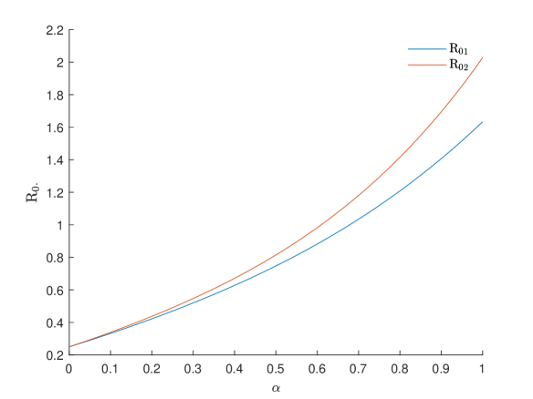
((a))

Figure 1: Impact of the variation of derivative order, $\alpha$, in the basic reproduction numbers of both communities (3) and (4), respectively, ${R_{0}}_{1}$ and ${R_{0}}_{2}$.

[See chitnis2008determining ; rodrigues2013sensitivity ] The normalised forward sensitivity index of ${R_{0}}_{i}$, which is differentiable with respect to a given parameter $p$, is defined by

$$\Upsilon_{p}^{{R_{0}}_{i}}=\frac{\partial{R_{0}}_{i}}{\partial p}\frac{p}{{R_{0}}_{i}},\quad{\scriptstyle i=1,2}.$$ (7)

Table 1 presents the values of the sensitivity index of the parameters of the model, obtained by the normalised sensitivity index (7), for the classical case ($\alpha=1$) of connected communities. These values have a meaning. For instance, $\Upsilon_{\varrho_{1}}^{{R_{0}}_{1}}=+0.999$ means that increasing (decreasing) $\varrho_{1}$ by a given percentage increases (decreases) always ${R_{0}}_{1}$ by nearly that same percentage. Sensitive parameters should be carefully evaluated, once a small perturbation in such parameter leads to significant quantitative changes. On the other hand, the estimation of a parameter with a small value for the sensitivity index does not require as much attention to evaluate, because a small perturbation in that parameter leads to small adjustments mikucki2012sensitivity . According with Table 1, we should pay special attention to the estimation of sensitive parameters $\varrho_{1}$ and $\varrho_{2}$. In contrast, the estimation of $K$, $\mu_{p}$, $\beta_{1}$, $\beta_{2}$, $\sigma_{1}$, $\sigma_{2}$, $g_{1}$, and $g_{2}$ do not require as much attention because of its low sensitivity. The missing parameters are those whose index value is zero.

[H] Sensitivity of ${R_{0}}_{1}$ (top) and ${R_{0}}_{2}$ (bottom), evaluated for the parameter values given in Table 3.1 with $\alpha=1$. Parameter $\Upsilon_{\cdot}^{{R_{0}}_{1}}$ Parameter $\Upsilon_{\cdot}^{{R_{0}}_{1}}$ Parameter $\Upsilon_{\cdot}^{{R_{0}}_{1}}$ $\pi_{1},\pi_{2}$ 0.500 $\mu_{2},a_{1}$ $-0.454$ $\beta_{1},\sigma_{1}$ $2\times 10^{-6}$ $\varrho_{1}$ 0.999 $K$ $-2\times 10^{-6}$ $\mu_{1}$ $-0.547$ $a_{2}$ 0.454 $b_{1}$ $-0.343$ $\delta_{1}$ $-0.143$ $\gamma_{1}$ $-0.514$ $\mu_{p}$ $-6\times 10^{-6}$ $g_{1}$ $4\times 10^{-6}$ Parameter $\Upsilon_{\cdot}^{{R_{0}}_{2}}$ Parameter $\Upsilon_{\cdot}^{{R_{0}}_{2}}$ Parameter $\Upsilon_{\cdot}^{{R_{0}}_{2}}$ $\pi_{1},\pi_{2}$ 0.500 $\mu_{2}$ $-0.456$ $\beta_{2},\sigma_{2}$ $1\times 10^{-5}$ $\varrho_{2}$ 0.999 $K$ $-1\times 10^{-5}$ $\mu_{1},a_{2}$ $-0.545$ $a_{1}$ 0.545 $b_{2}$ $-0.259$ $\delta_{2}$ $-0.416$ $\gamma_{2}$ $-0.324$ $\mu_{p}$ $-3\times 10^{-5}$ $g_{2}$ $2\times 10^{-5}$

For the fractional model, the sensitivity index depends on the derivative order $\alpha$. We can see this in Figure 2, where: (a) the impact of variation of $\alpha$ in the sensitivity index of $\beta_{1}$ is displayed for the first community; (b) the impact of variation of $\alpha$ in the sensitivity index of $\varrho_{2}$ is exhibited for the second community. The graphics of the other parameters are not shown because they exhibited similar behaviours. The parameters whose index value for $\alpha=1$ is close to zero, as $\beta_{1}$, do not vary much if we consider lower values of $\alpha$, as we see in Figure 2a. On the other hand, parameters whose index value in Table 1 are not as close to zero as the previous one, as $\varrho_{2}$, vary significantly if we consider lower values of $\alpha$, as we see in Figure 2b, and their sensitivity decreases with the decrease in $\alpha$.

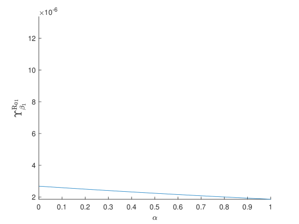
((a))

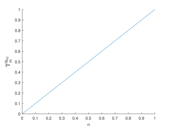
((b))

Figure 2: (a) Evolution of the sensitivity index of parameter $\beta_{1}$, evaluated for $\alpha$, with respect to ${R_{0}}_{1}$ (first community); (b) Evolution of the sensitivity index of parameter $\varrho_{2}$, evaluated for $\alpha$, with respect to ${R_{0}}_{2}$ (second community).

Figure 3 presents the evolution of the sensitivity index for the specific reproduction numbers of the two communities, ${R_{0}}_{1}$ and ${R_{0}}_{2}$, with the variation of the derivative order. We see that the evolution of the sensitivity index is analogous for the two reproduction numbers.

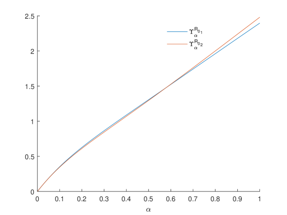
((a))

Figure 3: Evolution of the sensitivity index for the basic reproduction numbers of both communities, $R{{}_{0}}_{1}$ and ${R_{0}}_{2}$, with the variation of the derivative order, $\alpha$.

3.2 Fractional Optimal Control of the Model

Modelling dynamic control systems optimally is a very important issue in applied sciences and engineering MR4271051 . In this section, our aim is to minimise the number of cholera infected individuals and, simultaneously, to reduce the associated cost. This is achieved trough: (i) the use of vaccination into communities, as an effective time-dependent measure-control $v(t)$; (ii) the use of clean treated water, a preventive measure control $u(t)$; (iii) and the implementation of proper hygiene, another preventive measure control $m(t)$, in order to control person-to-person contact. Thus, we consider the following fractional optimal control problem:

$$\begin{split}\min~{}\mathcal{J}(I_{1},I_{2},u,v,&m)=\int_{0}^{t_{f}}\left(k_{1}I_{1}+k_{2}I_{2}+k_{3}u^{2}+k_{4}v^{2}+k_{5}m^{2}\right)~{}dt\\ \end{split}$$ (8)

subject to system (3)–(4) with given initial conditions

$$S_{1}(0)=S_{1_{0}}\geqslant 0,I_{1}(0)=I_{1_{0}}\geqslant 0,\ldots,R_{2}(0)=R_{2_{0}}\geqslant 0,B_{2}(0)=B_{2_{0}}\geqslant 0.$$ (9)

Note that we are using a quadratic cost functional on the controls, as an approximation to the real non-linear functional. Indeed, as in MyID:482 , our optimal control problem depends on the assumption that the cost takes a non-linear form. The parameters $0<k_{1},k_{2},k_{3},k_{4},k_{5}<+\infty$ are positive weights and $t_{f}$ is the duration of the control program. In addition, $k_{3},k_{4}$, and $k_{5}$ represent the costs of applying controls efforts $u$, $v$, and $m$, respectively. The set of admissible control functions is

$$\mathcal{U}=\left\{(u(\cdot),v(\cdot),m(\cdot))\in L^{\infty}(0,t_{f}):0\leqslant u\leqslant{u}_{\max},0\leqslant v\leqslant{v}_{\max},0\leqslant m\leqslant{m}_{\max}\right\}.$$ (10)

The Pontryagin maximum principle (PMP) for fractional optimal control is used to solve the problem MR3443073 ; MR4116679 . The Hamiltonian of the resulting optimal control problem is defined as

$$\begin{split}H&=k_{1}I_{1}+k_{2}I_{2}+k_{3}u^{2}+k_{4}v^{2}+k_{5}m^{2}+\xi_{1}\bigg{(}\pi_{1}^{\alpha}+a_{2}^{\alpha}S_{2}+\omega^{\alpha}R_{1}\\ &-(1-u)\dfrac{\beta_{1}^{\alpha}B_{1}S_{1}}{K+B_{1}}-(1-m)\varrho_{1}^{\alpha}I_{1}S_{1}-(a_{1}^{\alpha}+\mu_{1}^{\alpha}+v)S_{1}\bigg{)}\\[2.84526pt] &+\xi_{2}\left((1-u)\dfrac{\beta_{1}^{\alpha}B_{1}S_{1}}{K+B_{1}}+(1-m)\varrho_{1}^{\alpha}I_{1}S_{1}+b_{2}^{\alpha}I_{2}-Q_{1}I_{1}\right)\\[2.84526pt] &+\xi_{3}\left(vS_{1}+\gamma_{1}^{\alpha}I_{1}-(\mu_{1}^{\alpha}+\omega^{\alpha}+c_{1}^{\alpha})R_{1}+c_{2}^{\alpha}R_{2}\right)+\xi_{4}\left(\sigma_{1}^{\alpha}I_{1}-Q_{2}B_{1}\right)\\[2.84526pt] &+\xi_{5}\bigg{(}\pi_{2}^{\alpha}+a_{1}^{\alpha}S_{1}+\omega^{\alpha}R_{2}-(1-u)\dfrac{\beta_{2}^{\alpha}B_{2}S_{2}}{K+B_{2}}\\[2.84526pt] &-(1-m)\varrho_{2}^{\alpha}I_{2}S_{2}-(a_{2}^{\alpha}+\mu_{2}^{\alpha}+v)S_{2}\bigg{)}\\[2.84526pt] &+\xi_{6}\left((1-u)\dfrac{\beta_{2}^{\alpha}B_{2}S_{2}}{K+B_{2}}+(1-m)\varrho_{2}^{\alpha}I_{2}S_{2}+b_{1}^{\alpha}I_{1}-Q_{3}I_{2}\right)\\[2.84526pt] &+\xi_{7}\left(vS_{2}+\gamma_{2}^{\alpha}I_{2}-(\mu_{2}^{\alpha}+\omega^{\alpha}+c_{2}^{\alpha})R_{2}+c_{1}^{\alpha}R_{1}\right)+\xi_{8}\left(\sigma_{2}^{\alpha}I_{2}-Q_{4}B_{2}\right)\end{split}$$ (11)

and the adjoint system asserts that the co-state variables $\xi_{i}(t)$, $i=1,\ldots,8$, verify

$$\begin{split}{}^{\scriptscriptstyle C}_{\scriptscriptstyle 0}\!D^{\alpha}_{\scriptscriptstyle t}&\xi_{1}(t^{\prime})=\varrho_{1}^{\alpha}I_{1}(m-1)(\xi_{1}-\xi_{2})+a_{1}^{\alpha}(\xi_{5}-\xi_{1})\\ &+\frac{B_{1}\beta_{1}^{\alpha}(\xi_{1}-\xi_{2})(u-1)-B_{1}\mu_{1}^{\alpha}\xi_{1}-K\mu_{1}^{\alpha}\xi_{1}}{B_{1}+K}+(\xi_{3}-\xi_{1})v,\\[3.41432pt] {}^{\scriptscriptstyle C}_{\scriptscriptstyle 0}\!D^{\alpha}_{\scriptscriptstyle t}&\xi_{2}(t^{\prime})=k_{1}+\gamma_{1}^{\alpha}\xi_{3}+b_{1}^{\alpha}\xi_{6}+\varrho_{1}^{\alpha}(m-1)\xi_{1}S_{1}-\xi_{2}(Q_{1}+\varrho_{1}^{\alpha}(m-1)S_{1})\\ &+\xi_{4}\sigma_{1}^{\alpha},\\[3.41432pt] {}^{\scriptscriptstyle C}_{\scriptscriptstyle 0}\!D^{\alpha}_{\scriptscriptstyle t}&\xi_{3}(t^{\prime})=\omega^{\alpha}(\xi_{1}-\xi_{3})-(\mu_{1}^{\alpha}+c_{1}^{\alpha})\xi_{3}+c_{1}^{\alpha}\xi_{7},\\[3.41432pt] {}^{\scriptscriptstyle C}_{\scriptscriptstyle 0}\!D^{\alpha}_{\scriptscriptstyle t}&\xi_{4}(t^{\prime})=\frac{K(-K\xi_{4}Q_{2}+\beta_{1}^{\alpha}(\xi_{1}-\xi_{2})S_{1}(u-1))-B_{1}^{2}\xi_{4}Q_{2}-2B_{1}K\xi_{4}Q_{2}}{(B_{1}+K)^{2}},\\ {}^{\scriptscriptstyle C}_{\scriptscriptstyle 0}\!D^{\alpha}_{\scriptscriptstyle t}&\xi_{5}(t^{\prime})=a_{2}^{\alpha}(\xi_{1}-\xi_{5})+\varrho_{2}^{\alpha}I_{2}(m-1)(\xi_{5}-\xi_{6})\\ &+\frac{B_{2}\beta_{2}^{\alpha}(\xi_{5}-\xi_{6})(u-1)-B_{2}\mu_{2}^{\alpha}\xi_{5}-K\mu_{2}^{\alpha}\xi_{5}}{B_{2}+K}+(\xi_{7}-\xi_{5})v,\\ {}^{\scriptscriptstyle C}_{\scriptscriptstyle 0}\!D^{\alpha}_{\scriptscriptstyle t}&\xi_{6}(t^{\prime})=k_{2}+b_{2}^{\alpha}\xi_{2}+\gamma_{2}^{\alpha}\xi_{7}+\varrho_{2}^{\alpha}(m-1)\xi_{5}S_{2}-\xi_{6}(Q_{3}+\varrho_{2}^{\alpha}(m-1)S_{2})\\ &+\xi_{8}\sigma_{2}^{\alpha},\\ {}^{\scriptscriptstyle C}_{\scriptscriptstyle 0}\!D^{\alpha}_{\scriptscriptstyle t}&\xi_{7}(t^{\prime})=\omega^{\alpha}\xi_{5}+c_{2}^{\alpha}\xi_{3}-(\mu_{2}^{\alpha}+\omega^{\alpha}+c_{2}^{\alpha})\xi_{7},\\ {}^{\scriptscriptstyle C}_{\scriptscriptstyle 0}\!D^{\alpha}_{\scriptscriptstyle t}&\xi_{8}(t^{\prime})=\frac{K(-K\xi_{8}Q_{4}+\beta_{2}^{\alpha}(\xi_{5}-\xi_{6})S_{2}(u-1))-B_{2}^{2}\xi_{8}Q_{4}-2B_{2}K\xi_{8}Q_{4}}{(B_{2}+K)^{2}},\end{split}$$ (12)

with $t^{\prime}=t_{f}-t$. In turn, the optimality conditions of PMP establish that the optimal controls $u^{*}$, $v^{*}$, and $m^{*}$ are defined by

$$\begin{split}u^{*}&=\min\left\{\max\left\{0,\frac{B_{1}\beta_{1}^{\alpha}(\xi_{2}-\xi_{1})S_{1}}{2k_{3}(B_{1}+K)}+\frac{B_{2}\beta_{2}^{\alpha}(\xi_{6}-\xi_{5})S_{2}}{2k_{3}(B_{2}+K)}\right\},{u}_{\max}\right\},\\[5.69054pt] v^{*}&=\min\left\{\max\left\{0,\frac{S_{1}(\xi_{1}-\xi_{3})+S_{2}(\xi_{5}-\xi_{7})}{2k_{4}}\right\},{v}_{\max}\right\},\\[5.69054pt] m^{*}&=\min\left\{\max\left\{0,\frac{\varrho_{1}^{\alpha}I_{1}(\xi_{2}-\xi_{1})S_{1}+\varrho_{2}^{\alpha}I_{2}(\xi_{6}-\xi_{5})S_{2}}{2k_{5}}\right\},{m}_{\max}\right\}.\end{split}$$ (13)

In addition, the following transversality conditions hold:

$$\xi_{i}(t_{f})=0,\quad i=1,\ldots,8.$$ (14)

3.3 Numerical Results and Cost-Effectiveness Analysis

We start by calculating the relevance of the three measures used in the control of the disease. We do it by using the sensitivity index, presented in Definition 1, as proposed in 2019BpRL…14…27P . In this case, the sensitivity indices are presented as functions of the control parameters in Figure 4, using the parametric values from Table 3.1 and considering the classical model (that is, $\alpha=1$). The resulting graphics show that: (a) the curve of vaccination is the one that most rapidly moves away from zero, meaning that the vaccination program has a big impact for small rates of application; (b) proper hygiene measures are also important in the control of cholera, having a bigger impact for greater rates of application of it, being the only control that has precisely the same impact in both communities; (c) the domestic water treatment is useless in the control of cholera transmission, when used simultaneously with the two previous controls. So, in what follows, the third control, variable $u$, is ignored.

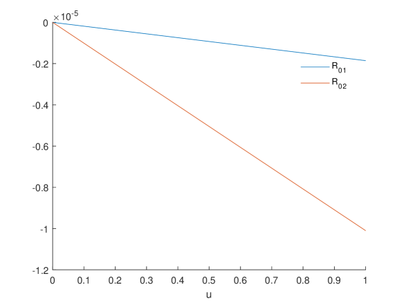
((a))

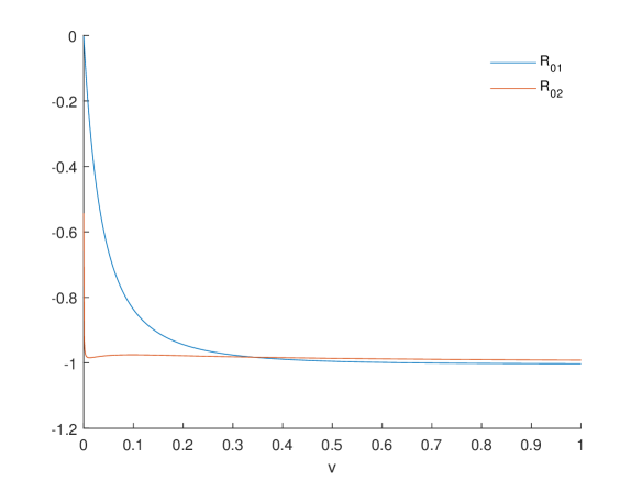
((b))

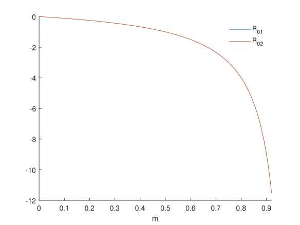
((c))

Figure 4: Sensitivity index of the basic reproduction numbers with respect to the control variables $u$ (top left), $v$ (top right), and $m$ (bottom).

One can deal with many different problems arising in different fields of sciences and engineering by applying some appropriate discretisation Ed4 . Here, the Pontryagin Maximum Principle is used to numerically solve the optimal control problem, as discussed in Section 3.2, both in classical and fractional cases, using the predict-evaluate-correct-evaluate (PECE) method of Adams–Basforth–Moulton diethelm2005algorithms , coded by us in MATLAB. Firstly, we solve system (3)–(4) by the PECE procedure, with the initial values for the state variables as given in Table 4 and a guess for the controls over the time interval $[0,t_{f}]$, that way obtaining the values of the state variables. Similarly to Rosa , a change of variable is applied to the adjoint system and to the transversality conditions, obtaining the fractional initial value problem (12)–(14). Such IVP is also solved with the PECE algorithm, and the values of the co-state variables $\xi_{i}$, $i=1,\ldots,8$, are determined. The controls are then updated by a convex combination of the controls of previous iteration and the current values, computed according to (13). This procedure is repeated iteratively until the values of all the variables and the values of the controls are almost identical to the ones of the previous iteration. The solutions of the classical model were successfully confirmed by a classical forward–backward scheme, also implemented by us in MATLAB.

In the numerical experiments, we consider weights $k_{1}=4$, $k_{2}=2.4$, $k_{3}=1.6$, and $k_{4}=k_{5}=1$. These values have the same relations between them than the homonyms weights in njagarah2015modelling , with the numerical advantage of being closer to the value one. We also use $v_{\max}=m_{\max}=1$, while the other parameters are fixed according to Table 3.1.

According with Figure 1, ${R_{0}}_{1}>1$ and ${R_{0}}_{2}>1$ for $\alpha\geqslant 0.68$ (endemic scenario). In order to be able to compare the FOCP results for several derivative orders, we consider the initial conditions, given by Table 4, which correspond to the non-trivial endemic equilibrium for system (3)–(4) for the classical cholera model ($\alpha=1$).

[H] Initial conditions for the fractional optimal control problem of Section 3.2 with parameters given by Table 3.1, corresponding to the endemic equilibrium of cholera model (3)–(4) with classical derivative order. $S_{1}(0)$ $I_{1}(0)$ $R_{1}(0)$ $B_{1}(0)$ $S_{2}(0)$ $I_{2}(0)$ $R_{2}(0)$ $B_{2}(0)$ 0.53144 0.001997 0.01028 0.30254 0.44222 0.002380 0.01082 0.36065

Without loss of generality, we consider the fractional order derivatives $\alpha=1.0$, $0.9$ and $0.8$. In Figures 5–7, we find the solutions of the fractional optimal control problem for those values of $\alpha$. We can see that a change in the value of $\alpha$ corresponds to significant variations of the state and control variables. Beyond those values of $\alpha$, others values were also tested, but the results do not changed qualitatively.

The efficacy function rodrigues2014cost , exhibited in Figure 8, is defined as

$$F(t)=\frac{i(0)-i^{*}(t)}{i(0)}=1-\frac{i^{*}(t)}{i(0)},$$ (15)

where $i^{*}(t)=I_{1}^{*}(t)+I_{2}^{*}(t)$ is the optimal solution associated with the fractional optimal control problem and $i(0)=I_{1}(0)+I_{2}(0)$ is the correspondent initial condition. This function measures the proportional variation in the number of infected individuals, of both communities, after the application of the control measures, $\{v^{*},m^{*}\}$, by comparing the number of infectious individuals at time $t$ with its initial value $i(0)$. We observe that the graphic of $F(t)$ exhibits the inverse tendency of infected individuals curves, growing and reaching the maximum at the end of the time interval.

To assess the cost and the effectiveness of the proposed fractional control measure during the intervention period, some summary measures are presented. The total cases averted by the intervention during the time period $t_{f}$ is defined in rodrigues2014cost by

$$AV=t_{f}i(0)-\int_{0}^{t_{f}}i^{*}(t)~{}dt,$$ (16)

where $i^{*}(t)$ is the optimal solution associated with the fractional optimal controls and $i(0)$ is the correspondent initial condition. Note that this initial condition is obtained as the equilibrium proportion $\overline{i}$ of systems (3)–(4), which is independent of time, so that $t_{f}i(0)=\displaystyle\int_{0}^{t_{f}}\overline{i}~{}dt$ represents the total infectious cases over a given period of $t_{f}$ days.

Effectiveness is defined as the proportion of cases averted on the total possible cases under no intervention  rodrigues2014cost :

$$\overline{F}=\frac{AV}{i(0)t_{f}}=1-\frac{\displaystyle\int_{0}^{t_{f}}i^{*}(t)~{}dt}{i(0)t_{f}}.$$ (17)

The total cost associated with the intervention is defined in rodrigues2014cost by

$$TC=\int_{0}^{t_{f}}(C_{1}\,v^{*}(t)s^{*}(t)+C_{2}\,m^{*}(t)i^{*}(t))dt,$$ (18)

where $s^{*}(t)=S_{1}^{*}(t)+S_{2}^{*}(t)$ and $C_{i}$ corresponds to the per person unit cost of the two possible interventions: (i) vaccination at any time $t$ of susceptible individuals ($C_{1}$); and (ii) infected individuals practising proper hygiene ($C_{2}$). Following okosun2013optimal ; rodrigues2014cost , the average cost-effectiveness ratio is given by

$$ACER=\frac{TC}{AV}.$$ (19)

The cost-effectiveness measures are summarised in Table 3.3. The results show the effectiveness of controls to reduce cholera infectious individuals and the leadership in doing so by the classical model ($\alpha=1$). [H] Summary of cost-effectiveness measures for classical and fractional ($0<\alpha<1$) cholera disease optimal control problems. Parameters according to Tables 3.1 and 4 with $C_{1}=C_{2}=1.$ $\alpha$ $AV$ $TC$ $ACER$ $\overline{F}$ 1.0 0.316716 0.90049 2.84322 0.723582 0.9 0.297175 1.17595 3.95708 0.678938 0.8 0.280311 1.35978 4.85099 0.640408

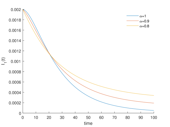
((a))

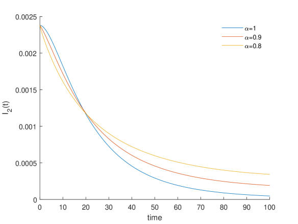
((b))

Figure 5: Variables $I_{1}$ and $I_{2}$ of the FOCP (8)–(13) with values from Table 3.1 and fractional order derivatives $\alpha=1.0,$ $0.9$ and $0.8$. (a) Evolution of infected individuals of 1st community; (b) Evolution of infected individuals of 2nd community.

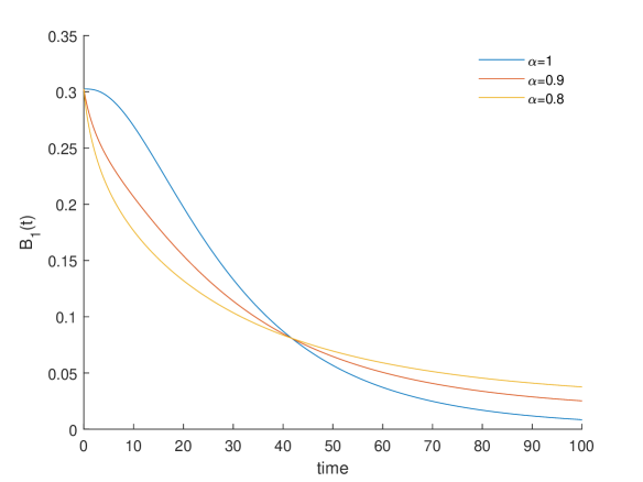
((a))

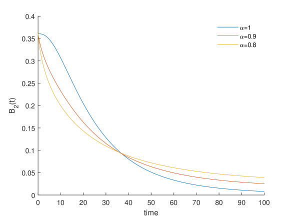
((b))

Figure 6: Variables $B_{1}$ and $B_{2}$ of the FOCP (8)–(13) with values from Table 3.1 and fractional order derivatives $\alpha=1.0$, $0.9$ and $0.8$. (a) Variation of vibrio population in 1st community; (b) Variation of vibrio population in 2nd community.

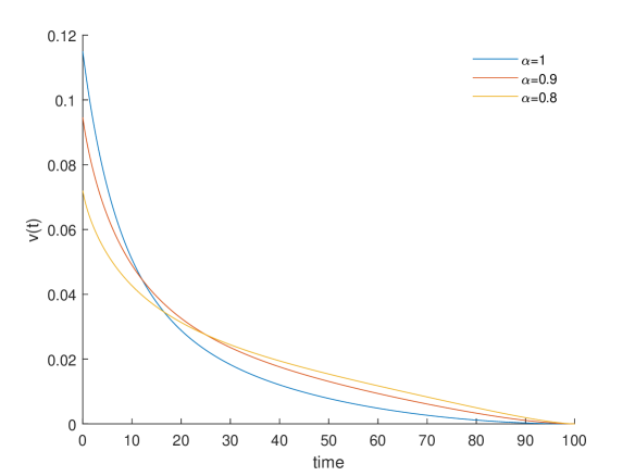
((a))

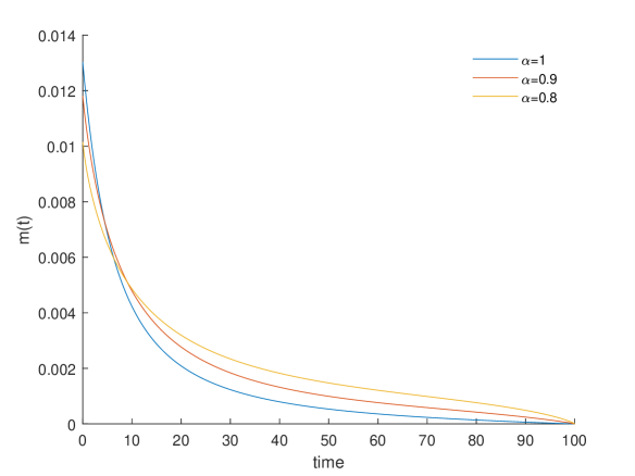
((b))

Figure 7: Control variables $v$ and $m$ of the FOCP (8)–(13) with values from Table 3.1 and fractional order derivatives $\alpha=1.0$, $0.9$ and $0.8$. (a) Contour of vaccination, $v$; (b) Evolution of control of hygiene, $m$.

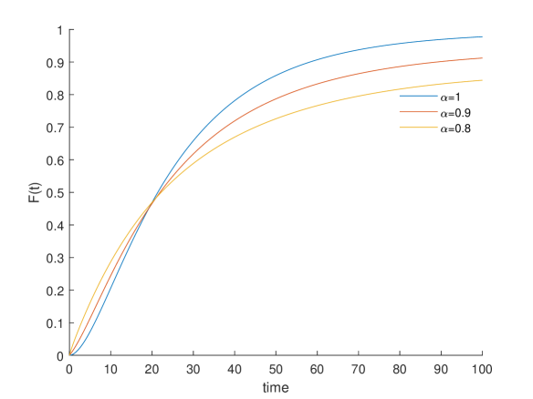
((a))

Figure 8: Evolution of the efficacy function (15) for the FOCP (8)–(13) with values from Table 3.1 and fractional order derivatives $\alpha=1.0,$ $0.9$ and $0.8$.

3.3.1 Optimal Control Strategies and Cost-Effectiveness Analysis

Now, we analyse the cost-effectiveness of alternative combinations of two possible control measures:

• strategy $A$—implementing the vaccination control, $v$;

• strategy $B$—implementing proper hygiene control, $m$;

• strategy $C$—implementing both controls, $v$ and $m$.

To analyse the cost-effectiveness of the three alternative strategies $A$, $B$, and $C$, we use the Incremental Cost-Effectiveness Ratio (ICER) okosun2013optimal . This ratio is used to compare the differences between costs and health outcomes of two alternative intervention strategies that compete for the same resources, being often described as the additional cost per additional health outcome. We start by ranking the strategies in order of increasing effectiveness, assessed by the total averted cases $AV$, defined in (16).

The ICER for the classical model ($\alpha=1$), is calculated as follows:

$$\begin{split}\mbox{ICER($B$)}=&\mbox{ACER}\mbox{($B$)}=0.216276,\\[2.84526pt] \mbox{ICER($A$)}=&\frac{0.900865-0.0084106}{0.316411-0.038888}=3.2157877,\\[2.84526pt] \mbox{ICER($C$)}=&\frac{1.900494-0.900865}{0.316716-0.316411}=-1.216393.\end{split}$$

Results are shown in Table 3.3.1. Strategy $A$ is the most costly one, so we exclude this strategy from the set of alternatives. We align the remaining strategies by increasing effectiveness ($AV$) and recalculate the ICER: $ICER(B)=ACER(B)=0.216276$ and $ICER(C)=3.210922$. Hence, we conclude that strategy $B$ (implementing only the control of hygiene measure, $m$) is the most cost-effective strategy. [H] Incremental cost-effectiveness ratio for strategies $A$, $B$, and $C$. Parameters according to Tables 3.1 and 4 with $C_{1}=C_{2}=1$ and $\alpha=1$. Strategies $AV$ $TC$ $ACER$ ICER $B$ 0.038888 0.0084106 0.216276 0.216276 $A$ 0.316411 0.900865 2.84713 3.2157877 $C$ 0.316716 0.900494 2.84322 $-1.216393$ The ICER was also computed for the fractional model, considering the same strategies, with the three derivative orders used previously: $\alpha=0.9$, $\alpha=0.8$ and $\alpha=0.68$. Even in those cases, we obtain the same conclusion: strategy $B$ is the most cost-effective.

Comparing the cost-effectiveness of strategy $B$ for above derivative orders, we start by getting the values of ICER presented in Table 3.3.1. Once the values of Total Cost (TC) diminish with the decrease in the derivative order, proceeding as above, when the values of ICER were computed for the classical $\alpha=1$ model, we eliminate successively the scheme with the highest TC. Consequently, the “strategies” $\alpha=1.0$, $\alpha=0.9$, and $\alpha=0.8$ are excluded, by this order.

Our conclusion is: the most cost-effective scheme is strategy $B$ with $\alpha=0.68$.

[H] Incremental cost-effectiveness ratio for strategy $B$ and several derivative orders. Same conditions as Table 3.3.1. $\alpha$ $AV$ $TC$ ICER 1.0 0.038888 0.0084106 0.216276 0.9 0.147496 0.003549 $-22.3419$ 0.8 0.203782 0.001705 $-30.5191$ 0.68 0.237211 0.000845 $-38.859$

3.3.2 The Variable-Order FractInt System

The solution of the Fractional Optimal Control Problem, exhibited in Section 3.3 for some derivative order values, evidences that the fractional-order model can be more effective in part of the time interval—as shown in Figure 8—but classical model is more effective if we consider all the interval, as shown in Table 3.3. In this section, we consider that the derivative order varies along the interval, being fractional or classical when more advantageous. According with Figure 8, $\alpha$ should be fractional at beginning and become classical/one after a certain time. Such class of Variable-Order Fractional (VOF) systems almeida2019variable are baptised here as FractInt. The derivative order of the FractInt system varies according with

$$\alpha(t)=\begin{cases}\alpha_{0}&\mbox{ if }0\leqslant t\leqslant t^{\prime},\\ 1&\mbox{ if }t^{\prime}<t\leqslant 100,\end{cases}$$ (20)

where $0<\alpha_{0}<1$. In practice, we noticed that the resulting system is as more effective as smaller the value of $\alpha_{0}$. In view of an endemic scenario, we consider in our simulations $\alpha_{0}=0.68$, which the lowest value that can guarantee it. With respect to the switching time, the value considered is $t^{\prime}=7$, which is the one to which it corresponds the maximum value of efficiency.

The FractInt system is numerically solved with the procedure described above, at the beginning of Section 3.3. In each iteration of the procedure, the predict-evaluate-correct-evaluate method is applied successively to each one of the two initial value problems—associated to the state system and to the adjoint system of the FOCP (8)–(13)—to perform the integration of them in two steps. These steps correspond to the two branches of the derivative order function, defined by (20). In such process, the final solution of first step (first branch) is the initial solution of the second step.

Solutions of the FractInt system are reproduced in Figures 9 and 10 along with solutions of the classical and fractional models ($\alpha=1$ and $\alpha=0.68$, respectively). We can see that the solutions of the FracInt system start to follow the solutions of the fractional model and end by following the solutions of the classical model. This behaviour can be observed in Figure 11, where the efficacy function for these three models is displayed.

The cost-effectiveness measures for the FractInt system are summarised in Table 3.3.2.

[H] Cost-effectiveness measures for the FractInt system. Parameters according to Tables 3.1 and 4 with $C_{1}=C_{2}=1$. $AV$ $TC$ $ACER$ $\overline{F}$ 0.332078 1.10967 3.3416 0.758679

Our results show that it is effective to control cholera infection through optimal control and that the FracInt model is more efficient than the classical one (cf. Table 3.3 and Figure 11), being the most effective model.

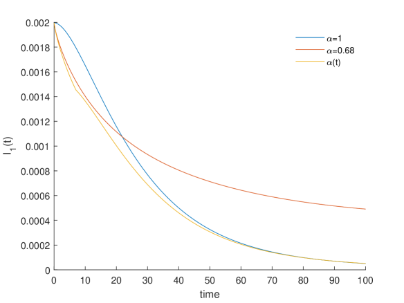
((a))

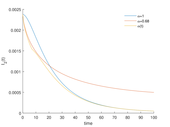
((b))

Figure 9: Comparison of variables $I_{1}$ and $I_{2}$ of the FractInt system with the ones of the FOCP (8)–(13) with $\alpha=1$ and $\alpha=0.68$, considering the parameter values from Table 3.1. (a) Infected individuals of 1st community; (b) Infected individuals of 2nd community.

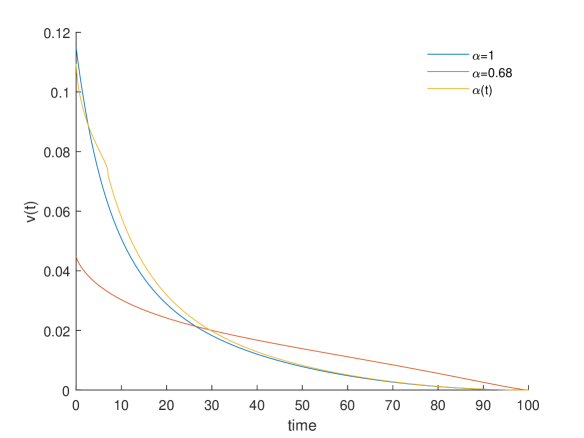
((a))

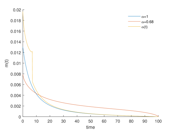
((b))

Figure 10: Comparison of variables $v$ and $m$ of the FractInt system with the ones of the FOCP (8)–(13) with $\alpha=1$ and $\alpha=0.68$, considering the parameter values from Table 3.1. (a) Contour of vaccination, $v$; (b) Evolution of the hygiene control, $m$.

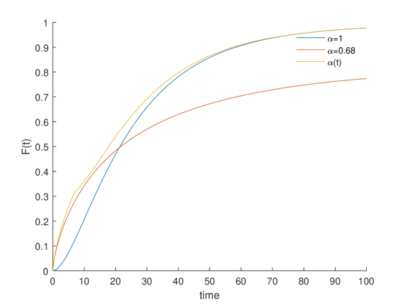
((a))

Figure 11: Evolution of the efficacy function for the FractInt system and for the FOCP with $\alpha=1$ and $\alpha=0.68$, considering the parameter values from Table 3.1.

4 Conclusions

Nowadays, Cholera infection is still an healthcare problem in many parts of the world, namely in impoverished regions where it has devastating effects. Its control is the goal of many studies in last years. In this work, a fractional-order mathematical model for Cholera with two connected communities, proposed in njagarah2018spatial , is studied and generalised. The two communities in appreciation are distinct and therefore they could not be molten in one unique community.

A sensitivity analysis of the model is done to show the importance of estimation of parameters. A fractional optimal control (FOC) problem is then formulated and numerically solved.

The relevance of studied controls is assessed using a cost-effectiveness analysis. Such analysis allow us to neglect the control $u$ (domestic water treatment) since it proved to be useless when used in combination with remaining controls.

The numerical results show that the FOC system is more effective only in part of the time interval. Therefore, we propose a system where the derivative order varies along the time interval, being fractional or integer when more advantageous in the control of infection. Such variable-order fractional model, baptised here as FractInt, shows to be the most effective in the control of the disease.

Conceptualisation, S.R. and D.F.M.T.; methodology, S.R. and D.F.M.T.; software, S.R.; validation, S.R. and D.F.M.T.; formal analysis, S.R. and D.F.M.T.; investigation, S.R. and D.F.M.T.; writing—original draft preparation, S.R. and D.F.M.T.; writing—review and editing, S.R. and D.F.M.T.; visualisation, S.R. and D.F.M.T. All authors have read and agreed to the published version of the manuscript.

This research was funded by Fundação para a Ciência e a Tecnologia (FCT, the Portuguese Foundation for Science and Technology) through IT, Grant Number UIDB/50008/2020 (S.R.), and CIDMA, Grant Number UIDB/04106/2020 (D.F.M.T.).

Not applicable.

Not applicable.

Not applicable.

- (1) Podlubny, I. Fractional Differential Equations; Mathematics in Science and Engineering; Academic Press, Inc.: San Diego, CA, USA, 1999; Volume 198.
- (2) Arqub, O.A. Computational algorithm for solving singular Fredholm time-fractional partial integrodifferential equations with error estimates. J. Appl. Math. Comput. 2019, 59, 227–243.
- (3) Djennadi, S.; Shawagfeh, N.; Abu Arqub, O. A fractional Tikhonov regularization method for an inverse backward and source problems in the time-space fractional diffusion equations. Chaos Solitons Fractals 2021, 150, 111127.
- (4) Mukandavire, Z.; Liao, S.; Wang, J.; Gaff, H.; Smith, D.L.; Morris, J.G. Estimating the reproductive numbers for the 2008–2009 Cholera outbreaks in Zimbabwe. Proc. Natl. Acad. Sci. USA 2011, 108, 8767–8772.
- (5) Lemos-Paião, A.P.; Silva, C.J.; Torres, D.F.M. An epidemic model for cholera with optimal control treatment. J. Comput. Appl. Math. 2017, 318, 168–180. arXiv:1611.02195
- (6) Lemos-Paião, A.P.; Silva, C.J.; Torres, D.F.M. A cholera mathematical model with vaccination and the biggest outbreak of world’s history. AIMS Math. 2018, 3, 448–463. arXiv:1810.05823
- (7) Lemos-Paião, A.P.; Silva, C.J.; Torres, D.F.M.; Venturino, E. Optimal control of aquatic diseases: A case study of Yemen’s cholera outbreak. J. Optim. Theory Appl. 2020, 185, 1008–1030. arXiv:2004.07402
- (8) Codeço, C.T. Endemic and epidemic dynamics of Cholera: The role of the aquatic reservoir. BMC Infect. Diseases 2001, 1, 14.
- (9) Capasso, V.; Paveri-Fontana, S. Mathematical model for the 1973 Cholera epidemic in the european mediterranean region. Revue d’Epidemiologie et de Sante Publique 1979, 27, 121–132.
- (10) Njagarah, J.B.H.; Tabi, C.B. Spatial synchrony in fractional order metapopulation Cholera transmission. Chaos Solitons Fractals 2018, 117, 37–49.
- (11) Njagarah, J.B.H.; Nyabadza, F. Modelling optimal control of Cholera in communities linked by migration. Comput. Math. Methods Med. 2015, 2015, 898264.
- (12) RNeilan, L.M.; Schaefer, E.; Gaff, H.; Fister, K.R.; Lenhart, S. Modeling optimal intervention strategies for Cholera. Bull. Math. Biol. 2010, 72, 2004–2018.
- (13) Boukhouima, A.; Lotfi, E.M.; Mahrouf, M.; Rosa, S.; Torres, D.F.M.; Yousfi, N. Stability analysis and optimal control of a fractional HIV-AIDS epidemic model with memory and general incidence rate. Eur. Phys. J. Plus 2021, 136, Art. 103, 1–20. arXiv:2012.04819
- (14) Ndaïrou, F.; Torres, D.F.M. Mathematical analysis of a fractional COVID-19 model applied to Wuhan, Spain and Portugal. Axioms 2021, 10, Art. 135, 1–13. arXiv:2106.15407
- (15) Ammi, M.R.S.; Tahiri, M.; Torres, D.F.M. Global stability of a Caputo fractional SIRS model with general incidence rate. Math. Comput. Sci. 2021, 15, 91–105. arXiv:2002.02560
- (16) Rosa, S.; Torres, D.F.M. Optimal control of a fractional order epidemic model with application to human respiratory syncytial virus infection. Chaos Solitons Fractals 2018, 117, 142–149. arXiv:1810.06900
- (17) Almeida, R. Analysis of a fractional SEIR model with treatment. Appl. Math. Lett. 2018, 84, 56–62.
- (18) Carvalho, A.R.M.; Pinto, C.M.A. Immune response in HIV epidemics for distinct transmission rates and for saturated CTL response. Math. Model. Nat. Phenom. 2019, 14, 307.
- (19) van den Driessche, P.; Watmough, J. Reproduction numbers and sub-threshold endemic equilibria for compartmental models of disease transmission. 2002, 180, 29–48.
- (20) Statistics South Africa. Community Survey 2016 Provincial Profile: Kwazulu Natal. 2016. Available online: http://cs2016.statssa.gov.za/wp-content/uploads/2018/07/KZN.pdf (acessed on 23 July 2019).
- (21) Jamison, D.T.; Feachem, R.G.; Makgoba, M.W.; Bos, E.R.; Baingana, F.K.; Hofman, K.J.; Rogo, K.O. (Eds.) Disease and Mortality in Sub-Saharan Africa; World Bank Publications: Washington, DC, 2006.
- (22) Kumate, J.; Sepúlveda, J.; Gutiérrez, G. Cholera epidemiology in latin america and perspectives for eradication. Bull. l’Institut Pasteur 1998, 96, 217–226.
- (23) King, A.A.; Ionides, E.L.; Pascual, M.; Bouma, M.J. Inapparent infections and Cholera dynamics. Nature 2008, 454, 877–880.
- (24) Hartley, D.M.; Morris, J.G., Jr.; Smith, D.L. Hyperinfectivity: A critical element in the ability of v. cholerae to cause epidemics? PLoS Med. 2005, 3, 7.
- (25) Mukandavire, Z.; Tripathi, A.; Chiyaka, C.; Musuka, G.; Nyabadza, F.; Mwambi, H. Modelling and analysis of the intrinsic dynamics of Cholera. Differ. Equ. Dyn. Syst. 2011, 19, 253–265.
- (26) Munro, P.M.; Colwell, R.R. Fate of vibrio Cholerae o1 in seawater microcosms. Water Res. 1996, 30, 47–50.
- (27) Chitnis, N.; Hyman, J.M.; Cushing, J.M. Determining important parameters in the spread of malaria through the sensitivity analysis of a mathematical model. Bull. Math. Biol. 2008, 70, 1272–1296.
- (28) Rodrigues, H.S.; Monteiro, M.T.T.; Torres, D.F.M. Sensitivity analysis in a dengue epidemiological model. Conf. Pap. Math. 2013, 2013, Art. 721406, 1–7. arXiv:1307.0202
- (29) Mikucki, M.A. Sensitivity Analysis of the Basic Reproduction Number and Other Quantities for Infectious Disease Models. Ph.D. Thesis, Colorado State University, Fort Collins, CO, USA, 2012.
- (30) Arqub, O.A.; Shawagfeh, N. Solving optimal control problems of Fredholm constraint optimality via the reproducing kernel Hilbert space method with error estimates and convergence analysis. Math. Methods Appl. Sci. 2021, 44, 7915–7932.
- (31) Abraha, T.; al Basir, F.; Obsu, L.L.; Torres, D.F.M. Farming awareness based optimum interventions for crop pest control. Math. Biosci. Eng. 2021, 18, 5364–5391. arXiv:2106.08192
- (32) Almeida, R.; Pooseh, S.; Torres, D.F.M. Computational Methods in the Fractional Calculus of Variations; Imperial College Press: London, UK, 2015.
- (33) Bergounioux, M.; Bourdin, L. Pontryagin maximum principle for general Caputo fractional optimal control problems with Bolza cost and terminal constraints. ESAIM Control Optim. Calc. Var. 2020, 26, 35.
- (34) Panja, P. Optimal Control Analysis of a Cholera Epidemic Model. Biophys. Rev. Lett. 2019, 14, 27–48.
- (35) Arqub, O.A.; Rashaideh, H.; The RKHS method for numerical treatment for integrodifferential algebraic systems of temporal two-point BVPs. Neural Comput. Appl. 2018, 30, 2595–2606.
- (36) Diethelm, K.; Ford, N.J.; Freed, A.D.; Luchko, Y.; Algorithms for the fractional calculus: A selection of numerical methods. Comput. Methods Appl. Mech. Eng. 2005, 194, 743–773.
- (37) Rodrigues, P.; Silva, C.J.; Torres, D.F.M. Cost-effectiveness analysis of optimal control measures for tuberculosis. Bull. Math. Biol. 2014, 76, 2627–2645. arXiv:1409.3496
- (38) Okosun, K.O.; Rachid, O.; Marcus, N. Optimal control strategies and cost-effectiveness analysis of a malaria model. BioSystems 2013, 111, 83–101.
- (39) Almeida, R.; Tavares, D.; Torres, D.F.M. The Variable-Order Fractional Calculus of Variations; Springer: Cham, Switzerland, 2019. arXiv:1805.00720