Random access test as an identifier of nonclassicality

Teiko Heinosaari  and  Leevi Leppäjärvi Teiko Heinosaari: teiko.heinosaari@utu.fi Leevi Leppäjärvi: leevi.leppajarvi@gmail.com (1) Department of Physics and Astronomy, University of Turku, Finland, (2) Quantum algorithms and software, VTT Technical Research Centre of Finland Ltd RCQI, Institute of Physics, Slovak Academy of Sciences, Dúbravská cesta 9, 84511 Bratislava, Slovakia
Abstract.

Random access codes are an intriguing class of communication tasks that reveal an operational and quantitative difference between classical and quantum information processing. We formulate a natural generalization of random access codes and call them random access tests, defined for any finite collection of measurements in an arbitrary finite dimensional general probabilistic theory. These tests can be used to examine collective properties of collections of measurements. We show that the violation of a classical bound in a random access test is a signature of either measurement incompatibility or super information storability. The polygon theories are exhaustively analyzed and a critical difference between even and odd polygon theories is revealed.

[Uncaptioned image]

1. Introduction

The central theoretical aim of quantum information processing is to understand how quantum physics can be exploited in computing and communication. For example, in the celebrated superdense coding protocol quantum entanglement is used to communicate a certain number of bits of information by transmitting smaller number of qubits and sharing beforehand entangled qubits [1]. In general, quantum protocols are superior to classical protocols in some information processing tasks, but not in all (such as in nonlocal computation [2] and some quantum guessing games [3]). Every task showing a quantum advantage also reveals something about quantum theory itself, although the quantum resources behind the advantage may not always be so straightforward to identify.

Random access codes (RACs) are simple communication protocols where a number of bits are encoded into a smaller number of bits and it is later randomly decided which bit should be decoded. This kind of tasks become interesting when compared to their quantum versions, known as quantum random access codes (QRACs), where a number of bits are encoded into a smaller number of qubits, or more generally, a quantum system with smaller dimension than the dimension of the classical encoding space [4, 5]. It is known that in many cases a quantum system is better than a classical system of the same operational dimension (i.e. with the same maximal number of perfectly distinguishable states), and quantum random access codes have been investigated from various different angles and generalized into different directions, see e.g. [6, 7, 8, 9]. It has been e.g. shown that QRAC provides a robust self-testing of mutually unbiased bases, which are the unique quantum measurements giving the optimal performance in a particular QRAC [10]. Further, it has been shown that to get any quantum advantage at all, one must use incompatible pair of measurements [11]. In that way, QRAC can be used as a semi-device independent certification of quantum incompatibility.

In the current investigation we adopt the approach started in [11] and generalize random access codes to random access tests (RATs) where the number of measurement outcomes and operational dimension of the communication medium are independent from each other (in RACs it is assumed that these are the same). We formulate random access tests in the framework of general probabilistic theories (GPTs), hence enabling us to compare the performances in different theories.

We connect the performance of a collection of measurements in a random access test to the decoding power of their specific approximate joint measurement, which we call the harmonic approximate joint measurement. This observation links the optimal performance of the RAT to the information storability of the full theory, a concept introduced in [12]. Remarkably, it is found that the measurement incompatibility is not a necessary condition for a performance over the classical bound (as it is in quantum theory), but also a phenomenon called super information storability can enable it. By super information storability we mean that the information storability is larger than the operational dimension of the theory; it’s existence was recognized and studied in [12].

We make a detailed investigation of the performance of RATs in polygon theories. The optimal performances reveal a difference between even and odd polygon theories and, perhaps more surprisingly, also a finer division into different classes in both polygons. Our investigation indicates that the optimal performance in information processing tasks is a route to a deeper understanding of GPTs and their nonclassical features, thereby also to a better understanding of quantum theory.

The present investigation is organized as follows. In Sec. 2 we recall the needed definitions and machinery of general probabilistic theories. Sec. 3 focuses on the concepts of decoding power of a measurement and information storability of a whole theory. In Sec. 4 we define a specific kind of approximate joint measurement for any collection of measurements, which turns out to be a useful tool. In Sec. 5 we are finally ready to define random access tests and show how they link to the earlier concepts. Sec. 6 connects the definite success of special random access tests to maximal incompatibility. In Sec. 7 we present a detailed study of random access tests in polygon state spaces and demonstrate how the maximal success probabilities separate different theories.

2. General probabilistic theories

General probabilistic theories constitutes a generalized framework for quantum and classical theories based on operational principles. In addition to quantum and classical theories, GPTs include countless toy theories where various operational features and tasks can be tested and considered in. This enables us to compare different theories to each other based on how these different features behave in different theories. In particular, by looking at the known nonclassical features of quantum theory (such as incompatibility [13, 14], steering [15, 16] and nonlocality [17, 18]) in this more general operational framework helps us understand what makes quantum theory special among all other possible theories. Furthermore, by looking at these features in the full scope of GPTs gives us insight on these features themselves which deepens our understanding about them and helps us make connections between different features.

GPTs are build around operational concepts such as preparations, transformations and measurements which are used to describe a physical experiment. The preparation procedure involves preparing a (physical) system in a state that contains the information about the system’s properties. The set of possible states is described by a state space 𝒮𝒮\mathcal{S} which is taken to be a compact convex subset of a finite-dimensional vector space 𝒱𝒱\mathcal{V}. Whereas compactness and finite-dimensionality are technical assumptions which are often made to simplify the mathematical treatment of the theory, convexity follows from the possibility to have probabilistic mixtures of different preparation devices: if we prepare the system in a state s1𝒮subscript𝑠1𝒮s_{1}\in\mathcal{S} with probability p[0,1]𝑝01p\in[0,1] or state s2𝒮subscript𝑠2𝒮s_{2}\in\mathcal{S} with probability 1p[0,1]1𝑝011-p\in[0,1] in different rounds of the experiment, then the prepared state is statistically described by the mixture ps1+(1p)s2𝑝subscript𝑠11𝑝subscript𝑠2ps_{1}+(1-p)s_{2} and must thus be a valid state in 𝒮𝒮\mathcal{S}. The extreme points of 𝒮𝒮\mathcal{S} are called pure and the set of pure states is described by 𝒮extsuperscript𝒮𝑒𝑥𝑡\mathcal{S}^{ext}. If a state is not pure then it is called mixed.

In the popular ordered vector space formalism (see e.g. [19, 20] for more details) the state space 𝒮𝒮\mathcal{S} is embedded as a compact convex base of a closed, generating proper cone 𝒱+subscript𝒱\mathcal{V}_{+} in a finite-dimensional ordered vector space 𝒱𝒱\mathcal{V}. This means that 𝒱+subscript𝒱\mathcal{V}_{+} is convex, it spans 𝒱𝒱\mathcal{V}, it satisfies 𝒱+𝒱+={0}\mathcal{V}_{+}\cap-\mathcal{V}_{+}=\{0\} and that every element x𝒱+{0}𝑥subscript𝒱0x\in\mathcal{V}_{+}\setminus\{0\} has a unique base decomposition x=αs𝑥𝛼𝑠x=\alpha s, where α>0𝛼0\alpha>0 and s𝒮𝑠𝒮s\in\mathcal{S}. In this case the state space can be expressed as

𝒮={x𝒱|x0,u(x)=1},𝒮conditional-set𝑥𝒱formulae-sequence𝑥0𝑢𝑥1\displaystyle\mathcal{S}=\{x\in\mathcal{V}\,|\,x\geq 0,\ u(x)=1\},

where the the partial order \geq in 𝒱𝒱\mathcal{V} is the partial order induced by the proper cone 𝒱+subscript𝒱\mathcal{V}_{+} defined in the usual way as xy𝑥𝑦x\geq y if and only if xy𝒱+𝑥𝑦subscript𝒱x-y\in\mathcal{V}_{+}, and u𝑢u is a order unit in the dual space 𝒱superscript𝒱\mathcal{V}^{*}, or equivalently, a strictly positive functional on 𝒱𝒱\mathcal{V}.

The measurement events are described by effects which are taken to be affine functionals from 𝒮𝒮\mathcal{S} to the interval [0,1]01[0,1]; for an effect e:𝒮[0,1]:𝑒𝒮01e:\mathcal{S}\to[0,1] we interpret e(s)𝑒𝑠e(s) as the probability that the measurement event corresponding to e𝑒e is detected when the system is in a state s𝒮𝑠𝒮s\in\mathcal{S}. The affinity of the effects follows from the statistical correspondence between states and effects according to which the effects respect the convex structure of the states so that

e(ps1+(1p)s2)=pe(s1)+(1p)e(s2)𝑒𝑝subscript𝑠11𝑝subscript𝑠2𝑝𝑒subscript𝑠11𝑝𝑒subscript𝑠2e(ps_{1}+(1-p)s_{2})=pe(s_{1})+(1-p)e(s_{2})

for all p[0,1]𝑝01p\in[0,1] and s1,s2𝒮subscript𝑠1subscript𝑠2𝒮s_{1},s_{2}\in\mathcal{S}.

The set of effects on a state space 𝒮𝒮\mathcal{S} is called the effect space of 𝒮𝒮\mathcal{S} and it is denoted by (𝒮)𝒮\mathcal{E}(\mathcal{S}). Two distinguished effects are the zero effect o𝑜o and the unit effect u𝑢u for which o(s)=0𝑜𝑠0o(s)=0 and u(s)=1𝑢𝑠1u(s)=1 for all s𝒮𝑠𝒮s\in\mathcal{S}. The effect space is clearly convex, and again the extreme elements of (𝒮)𝒮\mathcal{E}(\mathcal{S}) are called pure and others are mixed. The set of pure effects on a state space 𝒮𝒮\mathcal{S} is denoted by ext(𝒮)superscript𝑒𝑥𝑡𝒮\mathcal{E}^{ext}(\mathcal{S}).

In the ordered vector space formalism we extent the effects to linear functionals and in this case we can depict the effect space as

(𝒮)=𝒱+(u𝒱+)={e𝒱|oeu},𝒮subscriptsuperscript𝒱𝑢subscriptsuperscript𝒱conditional-set𝑒superscript𝒱𝑜𝑒𝑢\displaystyle\mathcal{E}(\mathcal{S})=\mathcal{V}^{*}_{+}\cap(u-\mathcal{V}^{*}_{+})=\{e\in\mathcal{V}^{*}\,|\,o\leq e\leq u\},

where the partial order on the dual space 𝒱superscript𝒱\mathcal{V}^{*} is induced by the dual cone 𝒱+={f𝒱|f(x)0x𝒱+}subscriptsuperscript𝒱conditional-set𝑓superscript𝒱𝑓𝑥0for-all𝑥subscript𝒱\mathcal{V}^{*}_{+}=\{f\in\mathcal{V}^{*}\,|\,f(x)\geq 0\ \forall x\in\mathcal{V}_{+}\}.

An important class of effects is the set of indecomposable effects. Following [21] we say that a nonzero effect e(𝒮)𝑒𝒮e\in\mathcal{E}(\mathcal{S}) is indecomposable if the decomposition e=e1+e2𝑒subscript𝑒1subscript𝑒2e=e_{1}+e_{2} for some two nonzero effects e1,e2(𝒮)subscript𝑒1subscript𝑒2𝒮e_{1},e_{2}\in\mathcal{E}(\mathcal{S}) implies that e=c1e1=c2e2𝑒subscript𝑐1subscript𝑒1subscript𝑐2subscript𝑒2e=c_{1}e_{1}=c_{2}e_{2} for some c1,c2>0subscript𝑐1subscript𝑐20c_{1},c_{2}>0. It was shown in [21] that every effect can be expressed as a finite sum of indecomposable effect and that every indecomposable effect can be expressed as a positive multiple of a pure indecomposable effect. Geometrically indecomposable effects are exactly those that lie on the extreme rays of the dual cone 𝒱+subscriptsuperscript𝒱\mathcal{V}^{*}_{+}. We denote the set of indecomposable effects on 𝒮𝒮\mathcal{S} by ind(𝒮)subscript𝑖𝑛𝑑𝒮\mathcal{E}_{ind}(\mathcal{S}) and the set of pure indecomposable effects by indext(𝒮)subscriptsuperscript𝑒𝑥𝑡𝑖𝑛𝑑𝒮\mathcal{E}^{ext}_{ind}(\mathcal{S}).

A measurement on a state space 𝒮𝒮\mathcal{S} with a finite number of outcomes is a mapping 𝖬:x𝖬x:𝖬maps-to𝑥subscript𝖬𝑥\mathsf{M}:x\mapsto\mathsf{M}_{x} from a finite outcome set ΩΩ\Omega to the set of effects (𝒮)𝒮\mathcal{E}(\mathcal{S}) such that xΩ𝖬x(s)=1subscript𝑥Ωsubscript𝖬𝑥𝑠1\sum_{x\in\Omega}\mathsf{M}_{x}(s)=1 for all s𝒮𝑠𝒮s\in\mathcal{S}, or equivalently, xΩ𝖬x=usubscript𝑥Ωsubscript𝖬𝑥𝑢\sum_{x\in\Omega}\mathsf{M}_{x}=u. We interpret 𝖬x(s)subscript𝖬𝑥𝑠\mathsf{M}_{x}(s) as the probability that an outcome x𝑥x is obtained when the system in a state s𝒮𝑠𝒮s\in\mathcal{S} is measured with the measurement 𝖬𝖬\mathsf{M}. We denote the set of all measurements on 𝒮𝒮\mathcal{S} by (𝒮)𝒮\mathcal{M}(\mathcal{S}).

The set of measurements with a fixed outcome set is convex, and we denote the set of all extreme measurements with any outcome set by ext(𝒮)superscript𝑒𝑥𝑡𝒮\mathcal{M}^{ext}(\mathcal{S}). We say that an measurement is indecomposable if each of it’s nonzero effect is indecomposable. We denote the set of indecomposable measurements on 𝒮𝒮\mathcal{S} by ind(𝒮)subscript𝑖𝑛𝑑𝒮\mathcal{M}_{ind}(\mathcal{S}) and the set of indecomposable extreme measurements by indext(𝒮)subscriptsuperscript𝑒𝑥𝑡𝑖𝑛𝑑𝒮\mathcal{M}^{ext}_{ind}(\mathcal{S}). A measurement 𝖳𝖳\mathsf{T} with an outcome set ΩΩ\Omega is said to be trivial if it does not give any information about the measured state, i.e., it is of the form 𝖳x=pxusubscript𝖳𝑥subscript𝑝𝑥𝑢\mathsf{T}_{x}=p_{x}u for all xΩ𝑥Ωx\in\Omega for some probability distribution p:=(px)xΩassign𝑝subscriptsubscript𝑝𝑥𝑥Ωp:=(p_{x})_{x\in\Omega} on ΩΩ\Omega.

There are two basic ways of forming new measurements: mixing and post-processing. First, as pointed out above, the set of measurements with a fixed set of outcomes is convex and thus we can make convex mixtures of measurements: if 𝖬(1),,𝖬(n)superscript𝖬1superscript𝖬𝑛\mathsf{M}^{(1)},\ldots,\mathsf{M}^{(n)} are measurements with an outcome set ΩΩ\Omega and (pi)i=1nsuperscriptsubscriptsubscript𝑝𝑖𝑖1𝑛(p_{i})_{i=1}^{n} is a probability distribution, then i=1npi𝖬(i)superscriptsubscript𝑖1𝑛subscript𝑝𝑖superscript𝖬𝑖\sum_{i=1}^{n}p_{i}\mathsf{M}^{(i)} is a measurement with effects i=1npi𝖬x(i)superscriptsubscript𝑖1𝑛subscript𝑝𝑖subscriptsuperscript𝖬𝑖𝑥\sum_{i=1}^{n}p_{i}\mathsf{M}^{(i)}_{x} for all xΩ𝑥Ωx\in\Omega. Clearly, those measurements that cannot be written as a nontrivial mixture are the extreme measurements.

Second, we say that a measurement 𝖭𝖭\mathsf{N} with an outcome set ΛΛ\Lambda is a post-processing of a measurement 𝖬𝖬\mathsf{M} with an outcome set ΩΩ\Omega if there exists a stochastic matrix ν:=(νxy)xΩ,yΛassign𝜈subscriptsubscript𝜈𝑥𝑦formulae-sequence𝑥Ω𝑦Λ\nu:=(\nu_{xy})_{x\in\Omega,y\in\Lambda}, i.e., νxy0subscript𝜈𝑥𝑦0\nu_{xy}\geq 0 for all xΩ,yΛformulae-sequence𝑥Ω𝑦Λx\in\Omega,y\in\Lambda and yΛνxy=1subscript𝑦Λsubscript𝜈𝑥𝑦1\sum_{y\in\Lambda}\nu_{xy}=1 for all xΩ𝑥Ωx\in\Omega, such that

𝖭y=xΩνxy𝖬xsubscript𝖭𝑦subscript𝑥Ωsubscript𝜈𝑥𝑦subscript𝖬𝑥\displaystyle\mathsf{N}_{y}=\sum_{x\in\Omega}\nu_{xy}\mathsf{M}_{x}

for all yΛ𝑦Λy\in\Lambda. In this case we denote 𝖭=ν𝖬𝖭𝜈𝖬\mathsf{N}=\nu\circ\mathsf{M}. The post-processing relation defines a preorder on the set of measurements as follows: 𝖭𝖬precedes-or-equals𝖭𝖬\mathsf{N}\preceq\mathsf{M} if and only if 𝖭=ν𝖬𝖭𝜈𝖬\mathsf{N}=\nu\circ\mathsf{M} for some stochastic matrix ν𝜈\nu. The set of maximal elements in (𝒮)𝒮\mathcal{M}(\mathcal{S}) with respect to the post-processing preorder is known to be exactly the set of indecomposable measurements ind(𝒮)subscript𝑖𝑛𝑑𝒮\mathcal{M}_{ind}(\mathcal{S}) [22, 23].

Example 1 (Quantum theory).

Let \mathcal{H} be a d𝑑d-dimensional Hilbert space. We denote by ()\mathcal{L(H)} the algebra of linear operators on \mathcal{H} and by s()subscript𝑠\mathcal{L}_{s}(\mathcal{H}) the real vector space of self-adjoint operators on \mathcal{H}. The state space of a d𝑑d-dimensional quantum theory is defined as

𝒮()={ϱs()|ϱO,tr[ϱ]=1},𝒮conditional-setitalic-ϱsubscript𝑠formulae-sequenceitalic-ϱ𝑂trdelimited-[]italic-ϱ1\displaystyle\mathcal{S(H)}=\{\varrho\in\mathcal{L}_{s}(\mathcal{H})\,|\,\varrho\geq O,\ {\rm tr}\left[\varrho\right]=1\},

where O𝑂O is the zero-operator and the partial order is induced by the cone of positive semi-definite matrices according to which a self-adjoint matrix A𝐴A is positive semi-definite, AO𝐴𝑂A\geq O, if and only if φ|Aφ0inner-product𝜑𝐴𝜑0\left\langle\,\varphi\,|\,A\varphi\,\right\rangle\geq 0 for all φ𝜑\varphi\in\mathcal{H}. The pure states are exactly the rank-1 projections on \mathcal{H}.

The set of effects (𝒮())𝒮\mathcal{E}(\mathcal{S(H)}) can be shown (see e.g. [24]) to be isomorphic to the set ()\mathcal{E(H)} of self-adjoint operators bounded between O𝑂O and 𝟙1\mathbbm{1}, where 𝟙1\mathbbm{1} is the identity operator on \mathcal{H}, i.e.,

(𝒮())():={Es()|OE𝟙}.similar-to-or-equals𝒮assignconditional-set𝐸subscript𝑠𝑂𝐸1\displaystyle\mathcal{E}(\mathcal{S(H)})\simeq\mathcal{E(H)}:=\{E\in\mathcal{L}_{s}(\mathcal{H})\,|\,O\leq E\leq\mathbbm{1}\}.

The pure effects then correspond to the projections on \mathcal{H} and the indecomposable effects to the rank-1 effect operators.

Measurements with finite number of outcomes on \mathcal{H} are described by positive operator-valued measures (POVMs), i.e., maps of the form M:xM(x):𝑀maps-to𝑥𝑀𝑥M:x\mapsto M(x) from a finite outcome set ΩΩ\Omega to the set of effect operatos ()\mathcal{E(H)} such that xΩM(x)=𝟙subscript𝑥Ω𝑀𝑥1\sum_{x\in\Omega}M(x)=\mathbbm{1}. The indecomposable POVMs are those whose all nonzero effects are rank-1 operators.

3. Decoding power and information storability

3.1. Base norms and order unit norms

Let us start by introducing some more structure on GPTs that is needed in order to define decoding power and information storability (for more details on GPTs see e.g. [19, 20]). Let 𝒮𝒮\mathcal{S} be a state space on an ordered vector space 𝒱𝒱\mathcal{V}. On the vector spaces 𝒱𝒱\mathcal{V} and 𝒱superscript𝒱\mathcal{V}^{*} we can define two natural norms that are induced by the cones 𝒱+subscript𝒱\mathcal{V}_{+} and 𝒱+superscriptsubscript𝒱\mathcal{V}_{+}^{*} respectively. We will introduce them next.

In the ordered vector space 𝒱𝒱\mathcal{V} we have that 𝒮𝒮\mathcal{S} is a compact base of the closed, generating proper cone 𝒱+subscript𝒱\mathcal{V}_{+} so that in particular every element x𝒱𝑥𝒱x\in\mathcal{V} can be expressed as x=αyβz𝑥𝛼𝑦𝛽𝑧x=\alpha y-\beta z for some α,β0𝛼𝛽0\alpha,\beta\geq 0 and y,z𝒮𝑦𝑧𝒮y,z\in\mathcal{S}. The base norm 𝒱\left\|\cdot\right\|_{\mathcal{V}} on 𝒱𝒱\mathcal{V} is then defined as

x𝒱=inf{α+β|x=αyβz,α,β0,y,z𝒮}subscriptnorm𝑥𝒱infimumconditional-set𝛼𝛽formulae-sequence𝑥𝛼𝑦𝛽𝑧𝛼formulae-sequence𝛽0𝑦𝑧𝒮\displaystyle\left\|x\right\|_{\mathcal{V}}=\inf\{\alpha+\beta\,|\,\ x=\alpha y-\beta z,\ \alpha,\beta\geq 0,\ y,z\in\mathcal{S}\}

for all x𝒱𝑥𝒱x\in\mathcal{V}. It follows that if x𝒱+𝑥subscript𝒱x\in\mathcal{V}_{+}, then x𝒱=u(x)subscriptnorm𝑥𝒱𝑢𝑥\left\|x\right\|_{\mathcal{V}}=u(x). In particular we have that 𝒮={x𝒱+|x𝒱=1}𝒮conditional-set𝑥subscript𝒱subscriptnorm𝑥𝒱1\mathcal{S}=\{x\in\mathcal{V}_{+}\,|\,\left\|x\right\|_{\mathcal{V}}=1\}.

In the dual space 𝒱superscript𝒱\mathcal{V}^{*} we have the order unit u𝒱+𝑢subscriptsuperscript𝒱u\in\mathcal{V}^{*}_{+}, i.e., for every f𝒱𝑓superscript𝒱f\in\mathcal{V}^{*} there exists λ>0𝜆0\lambda>0 such that fλu𝑓𝜆𝑢f\leq\lambda u, so that we can define the order unit norm 𝒱\left\|\cdot\right\|_{\mathcal{V}^{*}} on 𝒱superscript𝒱\mathcal{V}^{*} as

f𝒱=inf{λ0|λufλu}subscriptnorm𝑓superscript𝒱infimumconditional-set𝜆0𝜆𝑢𝑓𝜆𝑢\displaystyle\left\|f\right\|_{\mathcal{V}^{*}}=\inf\{\lambda\geq 0\,|\,-\lambda u\leq f\leq\lambda u\}

for all f𝒱𝑓superscript𝒱f\in\mathcal{V}^{*}. It follows that (𝒮)={f𝒱+|f𝒱1}𝒮conditional-set𝑓subscriptsuperscript𝒱subscriptnorm𝑓superscript𝒱1\mathcal{E}(\mathcal{S})=\{f\in\mathcal{V}^{*}_{+}\,|\,\left\|f\right\|_{\mathcal{V}^{*}}\leq 1\}. Furthermore, it can be shown that the base and the order unit norm are dual to each other, i.e.,

x𝒱=supf𝒱1|f(x)|,f𝒱=supx𝒱1|f(x)|.formulae-sequencesubscriptnorm𝑥𝒱subscriptsupremumsubscriptnorm𝑓superscript𝒱1𝑓𝑥subscriptnorm𝑓superscript𝒱subscriptsupremumsubscriptnorm𝑥𝒱1𝑓𝑥\displaystyle\left\|x\right\|_{\mathcal{V}}=\sup_{\left\|f\right\|_{\mathcal{V}^{*}}\leq 1}|f(x)|,\qquad\left\|f\right\|_{\mathcal{V}^{*}}=\sup_{\left\|x\right\|_{\mathcal{V}}\leq 1}|f(x)|.

In particular, we can express the order unit norm on 𝒱superscript𝒱\mathcal{V}^{*} as the supremum norm over 𝒮𝒮\mathcal{S} so that

f𝒱=sups𝒮|f(s)|subscriptnorm𝑓superscript𝒱subscriptsupremum𝑠𝒮𝑓𝑠\displaystyle\left\|f\right\|_{\mathcal{V}^{*}}=\sup_{s\in\mathcal{S}}|f(s)| (1)

for all f𝒱𝑓superscript𝒱f\in\mathcal{V}^{*}. Since 𝒮𝒮\mathcal{S} is compact, the supremum is always attained.

As we will mostly consider the properties of effects and measurements, we will be only using the norm 𝒱\left\|\cdot\right\|_{\mathcal{V}^{*}}. For this reason, in order to simplify our notation, from now on we will write \left\|\cdot\right\| instead of 𝒱\left\|\cdot\right\|_{\mathcal{V}^{*}}. We note that in particular for effects and other elements in 𝒱+subscriptsuperscript𝒱\mathcal{V}^{*}_{+} the absolute values in Eq. (1) can be removed, and thus we have that

e=maxs𝒮e(s)norm𝑒subscript𝑠𝒮𝑒𝑠\displaystyle\left\|e\right\|=\max_{s\in\mathcal{S}}e(s)

for all e𝒱+𝑒subscriptsuperscript𝒱e\in\mathcal{V}^{*}_{+}.

Example 2 (Quantum theory).

In the case of quantum theory 𝒮()𝒮\mathcal{S(H)} we note that for an effect e(𝒮())𝑒𝒮e\in\mathcal{E}(\mathcal{S(H)}) the norm enorm𝑒\left\|e\right\| corresponds to the operator norm Enorm𝐸\left\|E\right\| of the corresponding effect operator E()𝐸E\in\mathcal{E(H)}, which in the finite dimensional quantum theory equals with the maximal eigenvalue of E𝐸E.

3.2. Decoding power of a measurement

For a measurement 𝖬(𝒮)𝖬𝒮\mathsf{M}\in\mathcal{M}(\mathcal{S}) with an outcome set ΩΩ\Omega, we denote

λmax(𝖬):=xΩ𝖬x.assignsubscript𝜆𝑚𝑎𝑥𝖬subscript𝑥Ωnormsubscript𝖬𝑥\displaystyle\lambda_{max}(\mathsf{M}):=\sum_{x\in\Omega}\left\|\mathsf{M}_{x}\right\|\,.

An operational interpretation of λmax(𝖬)subscript𝜆𝑚𝑎𝑥𝖬\lambda_{max}(\mathsf{M}) is that two parties, a sender and a receiver, communicate by transferring physical systems where messages 1,,n1𝑛1,\ldots,n are encoded in states s1,,snsubscript𝑠1subscript𝑠𝑛s_{1},\ldots,s_{n}. The receiver is bound to use 𝖬𝖬\mathsf{M} to decode the messages, but the sender can freely choose the states. For each outcome x𝑥x of 𝖬𝖬\mathsf{M}, the sender hence chooses a state sxsubscript𝑠𝑥s_{x} such that the correct inference is as likely as possible, i.e., 𝖬x(sx)subscript𝖬𝑥subscript𝑠𝑥\mathsf{M}_{x}(s_{x}) is maximal. Assuming that the initial messages occur with uniform probability, the number λmax(𝖬)/nsubscript𝜆𝑚𝑎𝑥𝖬𝑛\lambda_{max}(\mathsf{M})/n is the maximal probability for the receiver to infer the correct messages by using 𝖬𝖬\mathsf{M}. Based on this operational motivation, we call λmax(𝖬)subscript𝜆𝑚𝑎𝑥𝖬\lambda_{max}(\mathsf{M}) the decoding power of 𝖬𝖬\mathsf{M}.

In the following we show that λmaxsubscript𝜆𝑚𝑎𝑥\lambda_{max} has certain monotonicity properties that makes it a reasonable quantification of the quality of measurements. In particular, we see that the decoding power function behaves in mixing and post-processing in the following way.

Proposition 1.

For any measurement 𝖬𝖬\mathsf{M} with an outcome set ΩΩ\Omega and post-processing ν=(νxy)xΩ,yΛ𝜈subscriptsubscript𝜈𝑥𝑦formulae-sequence𝑥Ω𝑦Λ\nu=(\nu_{xy})_{x\in\Omega,y\in\Lambda}, we have that

λmax(ν𝖬)λmax(𝖬).subscript𝜆𝑚𝑎𝑥𝜈𝖬subscript𝜆𝑚𝑎𝑥𝖬\displaystyle\lambda_{max}(\nu\circ\mathsf{M})\leq\lambda_{max}(\mathsf{M}).
Proof.

With a direct calculation by using the triangular inequality and the absolute homogenity of \left\|\cdot\right\| as well as the stochasticity of ν𝜈\nu we see that

λmax(ν𝖬)subscript𝜆𝑚𝑎𝑥𝜈𝖬\displaystyle\lambda_{max}(\nu\circ\mathsf{M}) =yΛ(ν𝖬)y=yΛxΩνxy𝖬xabsentsubscript𝑦Λnormsubscript𝜈𝖬𝑦subscript𝑦Λnormsubscript𝑥Ωsubscript𝜈𝑥𝑦subscript𝖬𝑥\displaystyle=\sum_{y\in\Lambda}\left\|(\nu\circ\mathsf{M})_{y}\right\|=\sum_{y\in\Lambda}\left\|\sum_{x\in\Omega}\nu_{xy}\mathsf{M}_{x}\right\|
yΛxΩνxy𝖬x=xΩ(yΛνxy)𝖬xabsentsubscript𝑦Λsubscript𝑥Ωsubscript𝜈𝑥𝑦normsubscript𝖬𝑥subscript𝑥Ωsubscript𝑦Λsubscript𝜈𝑥𝑦normsubscript𝖬𝑥\displaystyle\leq\sum_{y\in\Lambda}\sum_{x\in\Omega}\nu_{xy}\left\|\mathsf{M}_{x}\right\|=\sum_{x\in\Omega}\left(\sum_{y\in\Lambda}\nu_{xy}\right)\left\|\mathsf{M}_{x}\right\|
=xΩ𝖬x=λmax(𝖬).absentsubscript𝑥Ωnormsubscript𝖬𝑥subscript𝜆𝑚𝑎𝑥𝖬\displaystyle=\sum_{x\in\Omega}\left\|\mathsf{M}_{x}\right\|=\lambda_{max}(\mathsf{M})\,.

Proposition 2.

For any collection of measurements 𝖬(1),,𝖬(n)superscript𝖬1superscript𝖬𝑛\mathsf{M}^{(1)},\ldots,\mathsf{M}^{(n)} with an outcome set ΩΩ\Omega and probability distribution p:=(pi)i=1nassign𝑝superscriptsubscriptsubscript𝑝𝑖𝑖1𝑛p:=(p_{i})_{i=1}^{n} we have that

λmax(i=1npi𝖬(i))i=1npiλmax(𝖬(i))maxi{1,,n}λmax(𝖬(i)).subscript𝜆𝑚𝑎𝑥superscriptsubscript𝑖1𝑛subscript𝑝𝑖superscript𝖬𝑖superscriptsubscript𝑖1𝑛subscript𝑝𝑖subscript𝜆𝑚𝑎𝑥superscript𝖬𝑖subscript𝑖1𝑛subscript𝜆𝑚𝑎𝑥superscript𝖬𝑖\displaystyle\lambda_{max}\left(\sum_{i=1}^{n}p_{i}\mathsf{M}^{(i)}\right)\leq\sum_{i=1}^{n}p_{i}\lambda_{max}(\mathsf{M}^{(i)})\leq\max_{i\in\{1,\ldots,n\}}\lambda_{max}(\mathsf{M}^{(i)}).
Proof.

With a direct calculation by using the triangular inequality and the absolute homogenity of \left\|\cdot\right\| as well as the normalization of p𝑝p we see that

λmax(i=1npi𝖬(i))subscript𝜆𝑚𝑎𝑥superscriptsubscript𝑖1𝑛subscript𝑝𝑖superscript𝖬𝑖\displaystyle\lambda_{max}\left(\sum_{i=1}^{n}p_{i}\mathsf{M}^{(i)}\right) =xΩi=1npi𝖬x(i)xΩi=1npi𝖬x(i)absentsubscript𝑥Ωnormsuperscriptsubscript𝑖1𝑛subscript𝑝𝑖subscriptsuperscript𝖬𝑖𝑥subscript𝑥Ωsuperscriptsubscript𝑖1𝑛subscript𝑝𝑖normsubscriptsuperscript𝖬𝑖𝑥\displaystyle=\sum_{x\in\Omega}\left\|\sum_{i=1}^{n}p_{i}\mathsf{M}^{(i)}_{x}\right\|\leq\sum_{x\in\Omega}\sum_{i=1}^{n}p_{i}\left\|\mathsf{M}^{(i)}_{x}\right\|
=i=1npi(xΩ𝖬x(i))=i=1npiλmax(𝖬(i))absentsuperscriptsubscript𝑖1𝑛subscript𝑝𝑖subscript𝑥Ωnormsubscriptsuperscript𝖬𝑖𝑥superscriptsubscript𝑖1𝑛subscript𝑝𝑖subscript𝜆𝑚𝑎𝑥superscript𝖬𝑖\displaystyle=\sum_{i=1}^{n}p_{i}\left(\sum_{x\in\Omega}\left\|\mathsf{M}^{(i)}_{x}\right\|\right)=\sum_{i=1}^{n}p_{i}\lambda_{max}(\mathsf{M}^{(i)})
maxi{1,,n}λmax(𝖬(i)).absentsubscript𝑖1𝑛subscript𝜆𝑚𝑎𝑥superscript𝖬𝑖\displaystyle\leq\max_{i\in\{1,\ldots,n\}}\lambda_{max}(\mathsf{M}^{(i)}).

In the context of resource theories of measurements, the decoding power of a measurement is related to the robustness of measurements, defined as the minimal amount of noise needed to make a measurement trivial, studied in quantum theory e.g. in [25, 26] and in GPTs in [27].

3.3. Information storability

The previously defined decoding power is a quality of a single measurement. As we saw earlier, it is the maximal probability for a receiver to infer correct messages when the states used in encoding are optimized. We can also think of a scenario where the measurement is optimized over all possible measurements in the given theory. This quantity is known as the information storability [12] and for a theory with a state space 𝒮𝒮\mathcal{S} we denote it as

λmax((𝒮)):=sup𝖬(𝒮)λmax(𝖬).assignsubscript𝜆𝑚𝑎𝑥𝒮subscriptsupremum𝖬𝒮subscript𝜆𝑚𝑎𝑥𝖬\displaystyle\lambda_{max}(\mathcal{M}(\mathcal{S})):=\sup_{\mathsf{M}\in\mathcal{M}(\mathcal{S})}\lambda_{max}(\mathsf{M})\,. (2)

In the same way we can define the information storability for any subset 𝒯𝒯\mathcal{T} of measurements. This is particularly relevant when we study restrictions on measurements [28]. For a subset 𝒯(𝒮)𝒯𝒮\mathcal{T}\subseteq\mathcal{M}(\mathcal{S}) we denote the information storability of 𝒯𝒯\mathcal{T} as

λmax(𝒯):=sup𝖬𝒯λmax(𝖬).assignsubscript𝜆𝑚𝑎𝑥𝒯subscriptsupremum𝖬𝒯subscript𝜆𝑚𝑎𝑥𝖬\displaystyle\lambda_{max}(\mathcal{T}):=\sup_{\mathsf{M}\in\mathcal{T}}\lambda_{max}(\mathsf{M})\,.

In the cases where there is no risk of confusion we will use the simpler notation λmax(𝒮)subscript𝜆𝑚𝑎𝑥𝒮\lambda_{max}(\mathcal{S}) for λmax((𝒮))subscript𝜆𝑚𝑎𝑥𝒮\lambda_{max}(\mathcal{M}(\mathcal{S})).

Example 3 (Quantum theory).

In a finite d𝑑d-dimensional quantum theory for a POVM M𝑀M we have

λmax(M)=xM(x)xtr[M(x)]=tr[xM(x)]=tr[𝟙]=dsubscript𝜆𝑚𝑎𝑥𝑀subscript𝑥norm𝑀𝑥subscript𝑥trdelimited-[]𝑀𝑥trdelimited-[]subscript𝑥𝑀𝑥trdelimited-[]1𝑑\displaystyle\lambda_{max}(M)=\sum_{x}\left\|M(x)\right\|\leq\sum_{x}{\rm tr}\left[M(x)\right]={\rm tr}\left[\sum_{x}M(x)\right]={\rm tr}\left[\mathbbm{1}\right]=d

and we also see that this upper bound is reached whenever every operator M(x)𝑀𝑥M(x) is rank-1.

Based on Example 3 one could presume that the information storability is always the same as the operational dimension of the theory, as is the case for quantum theory. The latter dimension is defined as the maximal number of perfectly distinguishable states. The operational dimension of a theory clearly is a lower bound for the information storability. However, the information storability can be larger than the operational dimension and we call this phenomenon super information storability. This is the case e.g. in odd polygon theories (see Sec. 7).

From Prop. 1 and 2 it follows that the supremum in Eq. (2) is attained for extreme measurements that are maximal in the post-processing preorder. Thus, in a state space 𝒮𝒮\mathcal{S} we have that

λmax(𝒮)=sup𝖬(𝒮)λmax(𝖬)=sup𝖬indext(𝒮)λmax(𝖬).subscript𝜆𝑚𝑎𝑥𝒮subscriptsupremum𝖬𝒮subscript𝜆𝑚𝑎𝑥𝖬subscriptsupremum𝖬subscriptsuperscript𝑒𝑥𝑡𝑖𝑛𝑑𝒮subscript𝜆𝑚𝑎𝑥𝖬\displaystyle\lambda_{max}(\mathcal{S})=\sup_{\mathsf{M}\in\mathcal{M}(\mathcal{S})}\lambda_{max}(\mathsf{M})=\sup_{\mathsf{M}\in\mathcal{M}^{ext}_{ind}(\mathcal{S})}\lambda_{max}(\mathsf{M}). (3)

We note that the set of extreme indecomposable measurements indext(𝒮)subscriptsuperscript𝑒𝑥𝑡𝑖𝑛𝑑𝒮\mathcal{M}^{ext}_{ind}(\mathcal{S}) is exactly the set of extreme simulation irreducible measurements in [23].

For state spaces with a particular structure we can show a simple way of calculating the information storability of the theory. In particular, we will use this result for polygon state spaces in Sec. 7.

Proposition 3.

Suppose that there exists a state s0𝒮subscript𝑠0𝒮s_{0}\in\mathcal{S} such that e(s0)=f(s0)=:λ0e(s_{0})=f(s_{0})=:\lambda_{0} for all e,findext(𝒮)𝑒𝑓subscriptsuperscript𝑒𝑥𝑡𝑖𝑛𝑑𝒮e,f\in\mathcal{E}^{ext}_{ind}(\mathcal{S}). Then λmax(𝖬)=1/λ0subscript𝜆𝑚𝑎𝑥𝖬1subscript𝜆0\lambda_{max}(\mathsf{M})=1/\lambda_{0} for all 𝖬ind(𝒮)𝖬subscript𝑖𝑛𝑑𝒮\mathsf{M}\in\mathcal{M}_{ind}(\mathcal{S}) and therefore λmax(𝒮)=1/λ0subscript𝜆𝑚𝑎𝑥𝒮1subscript𝜆0\lambda_{max}(\mathcal{S})=1/\lambda_{0}.

Proof.

Let 𝖬ind(𝒮)𝖬subscript𝑖𝑛𝑑𝒮\mathsf{M}\in\mathcal{M}_{ind}(\mathcal{S}) with an outcome set ΩΩ\Omega. Since each effect 𝖬xsubscript𝖬𝑥\mathsf{M}_{x} is indecomposable, by [21] we have that 𝖬x=αxmxsubscript𝖬𝑥subscript𝛼𝑥subscript𝑚𝑥\mathsf{M}_{x}=\alpha_{x}m_{x} for some αx>0subscript𝛼𝑥0\alpha_{x}>0 and mxindext(𝒮)subscript𝑚𝑥subscriptsuperscript𝑒𝑥𝑡𝑖𝑛𝑑𝒮m_{x}\in\mathcal{E}^{ext}_{ind}(\mathcal{S}) for all xΩ𝑥Ωx\in\Omega. Furthermore, by [21], for all mxsubscript𝑚𝑥m_{x} there exists a pure state sx𝒮extsubscript𝑠𝑥superscript𝒮𝑒𝑥𝑡s_{x}\in\mathcal{S}^{ext} such that mx(sx)=1subscript𝑚𝑥subscript𝑠𝑥1m_{x}(s_{x})=1 so that 𝖬x=αxnormsubscript𝖬𝑥subscript𝛼𝑥\left\|\mathsf{M}_{x}\right\|=\alpha_{x} and λmax(𝖬)=xΩαxsubscript𝜆𝑚𝑎𝑥𝖬subscript𝑥Ωsubscript𝛼𝑥\lambda_{max}(\mathsf{M})=\sum_{x\in\Omega}\alpha_{x}.

From the normalization xΩ𝖬x=usubscript𝑥Ωsubscript𝖬𝑥𝑢\sum_{x\in\Omega}\mathsf{M}_{x}=u and the assumption that e(s0)=λ0𝑒subscript𝑠0subscript𝜆0e(s_{0})=\lambda_{0} for all eindext(𝒮)𝑒subscriptsuperscript𝑒𝑥𝑡𝑖𝑛𝑑𝒮e\in\mathcal{E}^{ext}_{ind}(\mathcal{S}) it follows that

1λ0=1λ0u(s0)=1λ0xΩαxmx(s0)=xΩαx=λmax(𝖬).1subscript𝜆01subscript𝜆0𝑢subscript𝑠01subscript𝜆0subscript𝑥Ωsubscript𝛼𝑥subscript𝑚𝑥subscript𝑠0subscript𝑥Ωsubscript𝛼𝑥subscript𝜆𝑚𝑎𝑥𝖬\displaystyle\dfrac{1}{\lambda_{0}}=\dfrac{1}{\lambda_{0}}u(s_{0})=\dfrac{1}{\lambda_{0}}\sum_{x\in\Omega}\alpha_{x}m_{x}(s_{0})=\sum_{x\in\Omega}\alpha_{x}=\lambda_{max}(\mathsf{M}).

The last claim follows from this and Eq. (3). ∎

4. Harmonic approximate joint measurements

A joint measurement of measurements 𝖬(1),,𝖬(k)superscript𝖬1superscript𝖬𝑘\mathsf{M}^{(1)},\ldots,\mathsf{M}^{(k)} with outcome sets Ω1,,ΩksubscriptΩ1subscriptΩ𝑘\Omega_{1},\ldots,\Omega_{k} is a measurement 𝖩𝖩\mathsf{J} with the product outcome set Ω1××ΩksubscriptΩ1subscriptΩ𝑘\Omega_{1}\times\cdots\times\Omega_{k} and satisfying the marginal properties

x2Ω2xkΩk𝖩x1,,xksubscriptsubscript𝑥2subscriptΩ2subscriptsubscript𝑥𝑘subscriptΩ𝑘subscript𝖩subscript𝑥1subscript𝑥𝑘\displaystyle\sum_{x_{2}\in\Omega_{2}}\cdots\sum_{x_{k}\in\Omega_{k}}\mathsf{J}_{x_{1},\ldots,x_{k}} =𝖬x1(1)x1Ω1,formulae-sequenceabsentsubscriptsuperscript𝖬1subscript𝑥1for-allsubscript𝑥1subscriptΩ1\displaystyle=\mathsf{M}^{(1)}_{x_{1}}\quad\forall x_{1}\in\Omega_{1},
\displaystyle\vdots\qquad
x1Ω1xk1Ωk1𝖩x1,,xksubscriptsubscript𝑥1subscriptΩ1subscriptsubscript𝑥𝑘1subscriptΩ𝑘1subscript𝖩subscript𝑥1subscript𝑥𝑘\displaystyle\sum_{x_{1}\in\Omega_{1}}\cdots\sum_{x_{k-1}\in\Omega_{k-1}}\mathsf{J}_{x_{1},\ldots,x_{k}} =𝖬xk(k)xkΩk.formulae-sequenceabsentsubscriptsuperscript𝖬𝑘subscript𝑥𝑘for-allsubscript𝑥𝑘subscriptΩ𝑘\displaystyle=\mathsf{M}^{(k)}_{x_{k}}\quad\forall x_{k}\in\Omega_{k}\,.

Measurements 𝖬(1),,𝖬(k)superscript𝖬1superscript𝖬𝑘\mathsf{M}^{(1)},\ldots,\mathsf{M}^{(k)} are called compatible if they have a joint measurement and otherwise they are incompatible.

In classical theories, i.e., in theories whose state spaces are simplices, all measurements are compatible whereas in every nonclassical GPTs there are pairs of measurements that are incompatible [29, 30]. However, even a set of incompatible measurements can be made incompatible if we allow for some amount of error. Most commonly this error is quantified by the amount of noise needed to be added to a set of incompatible set of measurements in order to make them compatible [13]. Formally, for each (λ1,,λk)[0,1]ksubscript𝜆1subscript𝜆𝑘superscript01𝑘(\lambda_{1},\ldots,\lambda_{k})\in[0,1]^{k} and every choice of trivial measurements 𝖳(1),,𝖳(k)superscript𝖳1superscript𝖳𝑘\mathsf{T}^{(1)},\ldots,\mathsf{T}^{(k)} the measurements λ1𝖬(1)+(1λ1)𝖳(1),,λk𝖬(k)+(1λk)𝖳(k)subscript𝜆1superscript𝖬11subscript𝜆1superscript𝖳1subscript𝜆𝑘superscript𝖬𝑘1subscript𝜆𝑘superscript𝖳𝑘\lambda_{1}\mathsf{M}^{(1)}+(1-\lambda_{1})\mathsf{T}^{(1)},\ldots,\lambda_{k}\mathsf{M}^{(k)}+(1-\lambda_{k})\mathsf{T}^{(k)} are considered to be noisy versions of the measurements 𝖬(1),,𝖬(k)superscript𝖬1superscript𝖬𝑘\mathsf{M}^{(1)},\ldots,\mathsf{M}^{(k)}, where the amount of noise added to each observable 𝖬(i)superscript𝖬𝑖\mathsf{M}^{(i)} is characterized by the parameter 1λi1subscript𝜆𝑖1-\lambda_{i}. In this case we call a joint measurement 𝖩~~𝖩\tilde{\mathsf{J}} of any noisy versions of the measurements 𝖬(1),,𝖬(k)superscript𝖬1superscript𝖬𝑘\mathsf{M}^{(1)},\ldots,\mathsf{M}^{(k)} an approximate joint measurement of 𝖬(1),,𝖬(k)superscript𝖬1superscript𝖬𝑘\mathsf{M}^{(1)},\ldots,\mathsf{M}^{(k)}.

Following [31] we can form a class of approximate joint measurements for 𝖬(1),,𝖬(k)superscript𝖬1superscript𝖬𝑘\mathsf{M}^{(1)},\ldots,\mathsf{M}^{(k)} by fixing convex weights λ1,,λksubscript𝜆1subscript𝜆𝑘\lambda_{1},\ldots,\lambda_{k} (so that λ1++λk=1subscript𝜆1subscript𝜆𝑘1\lambda_{1}+\cdots+\lambda_{k}=1) and probability distributions p(1),,p(k)superscript𝑝1superscript𝑝𝑘p^{(1)},\ldots,p^{(k)} on the sets Ω2××Ωk,,Ω1××Ωk1subscriptΩ2subscriptΩ𝑘subscriptΩ1subscriptΩ𝑘1\Omega_{2}\times\cdots\times\Omega_{k},\ldots,\Omega_{1}\times\cdots\times\Omega_{k-1} respectively and by setting

𝖩~x1,,xk=λ1px2,,xk(1)𝖬x1(1)++λkpx1,,xk1(k)𝖬xk(k)subscript~𝖩subscript𝑥1subscript𝑥𝑘subscript𝜆1subscriptsuperscript𝑝1subscript𝑥2subscript𝑥𝑘subscriptsuperscript𝖬1subscript𝑥1subscript𝜆𝑘subscriptsuperscript𝑝𝑘subscript𝑥1subscript𝑥𝑘1subscriptsuperscript𝖬𝑘subscript𝑥𝑘\displaystyle\tilde{\mathsf{J}}_{x_{1},\ldots,x_{k}}=\lambda_{1}p^{(1)}_{x_{2},\ldots,x_{k}}\mathsf{M}^{(1)}_{x_{1}}+\cdots+\lambda_{k}p^{(k)}_{x_{1},\ldots,x_{k-1}}\mathsf{M}^{(k)}_{x_{k}} (4)

for all (x1,,xk)Ω1××Ωksubscript𝑥1subscript𝑥𝑘subscriptΩ1subscriptΩ𝑘(x_{1},\ldots,x_{k})\in\Omega_{1}\times\cdots\times\Omega_{k}. The marginals of 𝖩~~𝖩\tilde{\mathsf{J}} are

x2Ω2xkΩk𝖩~x1,,xksubscriptsubscript𝑥2subscriptΩ2subscriptsubscript𝑥𝑘subscriptΩ𝑘subscript~𝖩subscript𝑥1subscript𝑥𝑘\displaystyle\sum_{x_{2}\in\Omega_{2}}\cdots\sum_{x_{k}\in\Omega_{k}}\tilde{\mathsf{J}}_{x_{1},\ldots,x_{k}} =λ1𝖬x1(1)+(1λ1)𝖳x1(1)x1Ω1,formulae-sequenceabsentsubscript𝜆1subscriptsuperscript𝖬1subscript𝑥11subscript𝜆1subscriptsuperscript𝖳1subscript𝑥1for-allsubscript𝑥1subscriptΩ1\displaystyle=\lambda_{1}\mathsf{M}^{(1)}_{x_{1}}+(1-\lambda_{1})\mathsf{T}^{(1)}_{x_{1}}\quad\forall x_{1}\in\Omega_{1},
\displaystyle\vdots\qquad
x1Ω1xk1Ωk1𝖩~x1,,xksubscriptsubscript𝑥1subscriptΩ1subscriptsubscript𝑥𝑘1subscriptΩ𝑘1subscript~𝖩subscript𝑥1subscript𝑥𝑘\displaystyle\sum_{x_{1}\in\Omega_{1}}\cdots\sum_{x_{k-1}\in\Omega_{k-1}}\tilde{\mathsf{J}}_{x_{1},\ldots,x_{k}} =λk𝖬xk(k)+(1λk)𝖳xk(k)xkΩk,formulae-sequenceabsentsubscript𝜆𝑘subscriptsuperscript𝖬𝑘subscript𝑥𝑘1subscript𝜆𝑘subscriptsuperscript𝖳𝑘subscript𝑥𝑘for-allsubscript𝑥𝑘subscriptΩ𝑘\displaystyle=\lambda_{k}\mathsf{M}^{(k)}_{x_{k}}+(1-\lambda_{k})\mathsf{T}^{(k)}_{x_{k}}\quad\forall x_{k}\in\Omega_{k},

where 𝖳(1),,𝖳(k)superscript𝖳1superscript𝖳𝑘\mathsf{T}^{(1)},\ldots,\mathsf{T}^{(k)} are trivial measurements.

In the previous construction we are free to choose the convex weights and the probability distributions. It turns out that a particular choice is useful for our following developments. We choose all probability distributions p(1),,p(k)superscript𝑝1superscript𝑝𝑘p^{(1)},\ldots,p^{(k)} to be uniform distributions and the convex weights are chosen to be

λi=h(m1,,mk)kmi,subscript𝜆𝑖subscript𝑚1subscript𝑚𝑘𝑘subscript𝑚𝑖\displaystyle\lambda_{i}=\frac{h(m_{1},...,m_{k})}{k\,m_{i}}\,,

where h(m1,,mk)subscript𝑚1subscript𝑚𝑘h(m_{1},\ldots,m_{k}) is the harmonic mean of the numbers m1,,mksubscript𝑚1subscript𝑚𝑘m_{1},\ldots,m_{k} and misubscript𝑚𝑖m_{i} is the number of outcomes of 𝖬(i)superscript𝖬𝑖\mathsf{M}^{(i)}. We denote this specific measurement as 𝖧(1,,k)superscript𝖧1𝑘\mathsf{H}^{(1,\ldots,k)} and call it harmonic approximate joint measurement of 𝖬(1),,𝖬(k)superscript𝖬1superscript𝖬𝑘\mathsf{M}^{(1)},\ldots,\mathsf{M}^{(k)}. Inserting the specific choices into Eq. (4) we observe that the harmonic approximate joint measurement can be written in the form

𝖧x1,,xk(1,,k)=1κ(m1,,mk)(𝖬x1(1)++𝖬xk(k)),subscriptsuperscript𝖧1𝑘subscript𝑥1subscript𝑥𝑘1𝜅subscript𝑚1subscript𝑚𝑘subscriptsuperscript𝖬1subscript𝑥1subscriptsuperscript𝖬𝑘subscript𝑥𝑘\displaystyle\mathsf{H}^{(1,\ldots,k)}_{x_{1},\ldots,x_{k}}=\frac{1}{\kappa(m_{1},\ldots,m_{k})}(\mathsf{M}^{(1)}_{x_{1}}+\cdots+\mathsf{M}^{(k)}_{x_{k}})\,, (5)

for all (x1,,xk)Ω1××Ωksubscript𝑥1subscript𝑥𝑘subscriptΩ1subscriptΩ𝑘(x_{1},\ldots,x_{k})\in\Omega_{1}\times\cdots\times\Omega_{k} with

κ(m1,,mk):=imii1mi.assign𝜅subscript𝑚1subscript𝑚𝑘subscriptproduct𝑖subscript𝑚𝑖subscript𝑖1subscript𝑚𝑖\displaystyle\kappa(m_{1},\ldots,m_{k}):=\prod_{i}m_{i}\sum_{i}\frac{1}{m_{i}}\,.

We remark that any approximate joint measurement of the form of Eq. (4) can be obtained from 𝖬(1),,𝖬(k)superscript𝖬1superscript𝖬𝑘\mathsf{M}^{(1)},\ldots,\mathsf{M}^{(k)} by a suitable mixing and post-processing, hence can be simulated by using those measurements only [23]. In this sense, they are all trivial approximate joint measurements and among these trivial approximate joint measurements our specific choice 𝖧(1,,k)superscript𝖧1𝑘\mathsf{H}^{(1,\ldots,k)} stands out by having a particularly symmetric form. Although trivial approximate joint measurements can be formed for any collection of measurements, we will show that the harmonic approximate joint measurement 𝖧(1,,k)superscript𝖧1𝑘\mathsf{H}^{(1,\ldots,k)} is related to the incompatibility of 𝖬(1),,𝖬(k)superscript𝖬1superscript𝖬𝑘\mathsf{M}^{(1)},\ldots,\mathsf{M}^{(k)} in an intriguing way. The link is explained in the following sections.

5. Random access tests

5.1. Classical and quantum random access codes

As a motivation for the later developments, we recall that in the (n,d)𝑛𝑑(n,d)random access code (RAC), Alice is given n𝑛n input dits x=(x1,,xn){0,,d1}n𝑥subscript𝑥1subscript𝑥𝑛superscript0𝑑1𝑛\vec{x}=(x_{1},\ldots,x_{n})\in\{0,\ldots,d-1\}^{n} based on which she prepares one dit and sends it to Bob. Bob is then given a number j{1,,n}𝑗1𝑛j\in\{1,\ldots,n\} and the task of Bob is to guess the corresponding dit xjsubscript𝑥𝑗x_{j} of Alice. The temporal order is here important: Alice does not know j𝑗j and therefore cannot simply send xjsubscript𝑥𝑗x_{j} to Bob. It is clear that, assuming all inputs are sampled uniformly, Bob will make errors. The performance depends on the strategy that Alice and Bob agree to follow. The choices of the inputs given to Alice and Bob are sampled with uniform probability and the average success probability quantifies the quality of their strategy. Generally, we denote by P¯c(n,d)subscriptsuperscript¯𝑃𝑛𝑑𝑐\bar{P}^{(n,d)}_{c} the best average success probability that Alice and Bob can achieve with a coordinated strategy.

For instance, Alice and Bob can agree that Alice always sends the value of the first dit. If Bob has to announce the value of the first dit, he makes no errors. This happens with the probability 1/n1𝑛1/n. On the other hand, with the probaility (n1)/n𝑛1𝑛(n-1)/n Bob has to announce the value of some other dit in which case the information received from Alice does not help Bob and he has to make a random choice, thereby guessing the right value with the probability 1/d1𝑑1/d. Therefore, with this strategy the average success probability is (d+n1)/(nd)𝑑𝑛1𝑛𝑑(d+n-1)/(nd). It can be shown that in the case when n=2𝑛2n=2 this is also the optimal strategy so that P¯c(2,d)=1/2(1+1/d)subscriptsuperscript¯𝑃2𝑑𝑐1211𝑑\bar{P}^{(2,d)}_{c}=1/2(1+1/d) [32, 33].

In (n,d)𝑛𝑑(n,d)quantum random access code (QRAC), Alice is given n𝑛n input dits x=(x1,,xn){0,,d1}n𝑥subscript𝑥1subscript𝑥𝑛superscript0𝑑1𝑛\vec{x}=(x_{1},\ldots,x_{n})\in\{0,\ldots,d-1\}^{n} based on which she prepares a d𝑑d-dimensional quantum system into a state ϱx𝒮(d)subscriptitalic-ϱ𝑥𝒮subscript𝑑\varrho_{\vec{x}}\in\mathcal{S}(\mathcal{H}_{d}) and sends it to Bob. Bob is then given a number j{1,,n}𝑗1𝑛j\in\{1,\ldots,n\} and the task of Bob is to guess the corresponding dit xjsubscript𝑥𝑗x_{j} of Alice by performing a measurement on the state sent by Alice. If Bob performs a measurement described by a d𝑑d-outcome POVM M(j)superscript𝑀𝑗M^{(j)}, the average success probability of QRAC when the inputs are assumed to be uniformly distributed is given by

1ndnxtr[ϱx(M(1)(x1)++M(n)(xn))].1𝑛superscript𝑑𝑛subscript𝑥trdelimited-[]subscriptitalic-ϱ𝑥superscript𝑀1subscript𝑥1superscript𝑀𝑛subscript𝑥𝑛\displaystyle\dfrac{1}{nd^{n}}\sum_{\vec{x}}{\rm tr}\left[\varrho_{\vec{x}}(M^{(1)}(x_{1})+\cdots+M^{(n)}(x_{n}))\right].

The best average success probability P¯q(n,d)subscriptsuperscript¯𝑃𝑛𝑑𝑞\bar{P}^{(n,d)}_{q} of a (n,d)𝑛𝑑(n,d)-QRAC is then obtained by optimizing over the states and the measurements so that

P¯q(n,d)=supM(1),,M(n)(d)1ndnxM(1)(x1)++M(n)(xn),subscriptsuperscript¯𝑃𝑛𝑑𝑞subscriptsupremumsuperscript𝑀1superscript𝑀𝑛subscript𝑑1𝑛superscript𝑑𝑛subscript𝑥normsuperscript𝑀1subscript𝑥1superscript𝑀𝑛subscript𝑥𝑛\displaystyle\bar{P}^{(n,d)}_{q}=\sup_{M^{(1)},\ldots,M^{(n)}\in\mathcal{M}(\mathcal{H}_{d})}\dfrac{1}{nd^{n}}\sum_{\vec{x}}\left\|M^{(1)}(x_{1})+\cdots+M^{(n)}(x_{n})\right\|,

where the norm is the operator norm on (d)subscript𝑑\mathcal{L}(\mathcal{H}_{d}). In the case that n=2𝑛2n=2 it is known that P¯q(2,d)=1/2(1+1/d)>P¯c(2,d)subscriptsuperscript¯𝑃2𝑑𝑞1211𝑑subscriptsuperscript¯𝑃2𝑑𝑐\bar{P}^{(2,d)}_{q}=1/2(1+1/\sqrt{d})>\bar{P}^{(2,d)}_{c} and that this bound can only be attained with rank-1 projective and mutually unbiased POVMs [10].

5.2. Random access tests in GPTs

In the following we formulate a class of tests that are similar to QRACs but are free from certain assumptions. Instead of restricting the number of measurement outcomes to match the (operational) dimension of the theory, we look at tests where the number of outcomes can be arbitrary. Furthermore, we look at these tests from the point of view of testing properties of collections of measurements in a given GPT.

The tests are defined as follows: Let 𝒮𝒮\mathcal{S} be a state space and let 𝖬(1),,𝖬(k)superscript𝖬1superscript𝖬𝑘\mathsf{M}^{(1)},\ldots,\mathsf{M}^{(k)} be measurements on 𝒮𝒮\mathcal{S} with outcome sets Ω1,,ΩksubscriptΩ1subscriptΩ𝑘\Omega_{1},\ldots,\Omega_{k} with m1,,mksubscript𝑚1subscript𝑚𝑘m_{1},\ldots,m_{k} outcomes respectively. As in the QRAC setting, Alice prepares a state sx𝒮subscript𝑠𝑥𝒮s_{\vec{x}}\in\mathcal{S}, where x=(x1,,xk)Ω1××Ωk𝑥subscript𝑥1subscript𝑥𝑘subscriptΩ1subscriptΩ𝑘\vec{x}=(x_{1},\ldots,x_{k})\in\Omega_{1}\times\cdots\times\Omega_{k}. The task is the same as before: Bob is told an index j{1,,k}𝑗1𝑘j\in\{1,\ldots,k\} and he should guess the label xjsubscript𝑥𝑗x_{j} by performing a measurement 𝖬(j)superscript𝖬𝑗\mathsf{M}^{(j)} on the state sxsubscript𝑠𝑥s_{\vec{x}}. When the queries are uniformly distributed the average success probability of this random access test (RAT) is then

1km1mkx(𝖬x1(1)++𝖬xk(k))(sx).1𝑘subscript𝑚1subscript𝑚𝑘subscript𝑥superscriptsubscript𝖬subscript𝑥11subscriptsuperscript𝖬𝑘subscript𝑥𝑘subscript𝑠𝑥\displaystyle\frac{1}{km_{1}\cdots m_{k}}\sum_{\vec{x}}\left(\mathsf{M}_{x_{1}}^{(1)}+\cdots+\mathsf{M}^{(k)}_{x_{k}}\right)(s_{\vec{x}})\,.

When Bob is required to use the fixed measurements 𝖬(1),,𝖬(k)superscript𝖬1superscript𝖬𝑘\mathsf{M}^{(1)},\ldots,\mathsf{M}^{(k)} and one optimizes over the states, the maximum average success probability becomes

P¯(𝖬(1),,𝖬(k)):=1km1mkx𝖬x1(1)++𝖬xk(k),assign¯𝑃superscript𝖬1superscript𝖬𝑘1𝑘subscript𝑚1subscript𝑚𝑘subscript𝑥normsuperscriptsubscript𝖬subscript𝑥11subscriptsuperscript𝖬𝑘subscript𝑥𝑘\displaystyle\bar{P}(\mathsf{M}^{(1)},\ldots,\mathsf{M}^{(k)}):=\frac{1}{km_{1}\cdots m_{k}}\sum_{\vec{x}}\left\|\mathsf{M}_{x_{1}}^{(1)}+\cdots+\mathsf{M}^{(k)}_{x_{k}}\right\|, (6)

where the norm is now the order unit norm in the dual space 𝒱superscript𝒱\mathcal{V}^{*} of the ordered vector space 𝒱𝒱\mathcal{V} in which the state space 𝒮𝒮\mathcal{S} is embedded. The number P¯(𝖬(1),,𝖬(k))¯𝑃superscript𝖬1superscript𝖬𝑘\bar{P}(\mathsf{M}^{(1)},\ldots,\mathsf{M}^{(k)}) is therefore the maximal success probability of the test for Alice and Bob if they are bound to use the measurements 𝖬(1),,𝖬(k)superscript𝖬1superscript𝖬𝑘\mathsf{M}^{(1)},\ldots,\mathsf{M}^{(k)} but free to choose the states.

A direct calculation reveals the following formula.

Proposition 4.
P¯(𝖬(1),,𝖬(k))=1h(m1,,mk)λmax(𝖧(1,,k)).¯𝑃superscript𝖬1superscript𝖬𝑘1subscript𝑚1subscript𝑚𝑘subscript𝜆𝑚𝑎𝑥superscript𝖧1𝑘\displaystyle\bar{P}(\mathsf{M}^{(1)},\ldots,\mathsf{M}^{(k)})=\tfrac{1}{h(m_{1},\ldots,m_{k})}\,\lambda_{max}(\mathsf{H}^{(1,\ldots,k)})\,. (7)

This observation shows that the two operationally accessible quantities P¯(𝖬(1),,𝖬(k))¯𝑃superscript𝖬1superscript𝖬𝑘\bar{P}(\mathsf{M}^{(1)},\ldots,\mathsf{M}^{(k)}) and λmax(𝖧(1,,k))subscript𝜆𝑚𝑎𝑥superscript𝖧1𝑘\lambda_{max}(\mathsf{H}^{(1,\ldots,k)}) are connected in a simple way. However, let us emphasize that in real experiments one would find lower bounds for these quantities as they are defined via optimal states.

From Eq. (6) (or equivalently from Eq. (7)) one gets the following upper bound

P¯(𝖬(1),,𝖬(k))1ki=1kλmax(𝖬(i))mi.¯𝑃superscript𝖬1superscript𝖬𝑘1𝑘superscriptsubscript𝑖1𝑘subscript𝜆𝑚𝑎𝑥superscript𝖬𝑖subscript𝑚𝑖\displaystyle\bar{P}(\mathsf{M}^{(1)},\ldots,\mathsf{M}^{(k)})\leq\frac{1}{k}\sum_{i=1}^{k}\frac{\lambda_{max}(\mathsf{M}^{(i)})}{m_{i}}\,.

Thus, the maximum average success probability of a random access test is upper bounded by the weighted average of the decoding powers of the measurements used in the test. Clearly λmax(𝖬(i))misubscript𝜆𝑚𝑎𝑥superscript𝖬𝑖subscript𝑚𝑖\lambda_{max}(\mathsf{M}^{(i)})\leq m_{i} for all i{1,,k}𝑖1𝑘i\in\{1,\ldots,k\}, where the equality holds only when 𝖬(i)superscript𝖬𝑖\mathsf{M}^{(i)} perfectly distinguishes misubscript𝑚𝑖m_{i} (not necessarily different) states which is the only case when the bound is trivial. However, we note that in order to calculate this bound one has to be familiar with the description of the measurements 𝖬(1),,𝖬(k)superscript𝖬1superscript𝖬𝑘\mathsf{M}^{(1)},\ldots,\mathsf{M}^{(k)}.

On the other hand, if we do not know the exact specification of the measurements but only know that 𝖬(1),,𝖬(k)superscript𝖬1superscript𝖬𝑘\mathsf{M}^{(1)},\ldots,\mathsf{M}^{(k)} belong to a set 𝒯(𝒮)𝒯𝒮\mathcal{T}\subseteq\mathcal{M}(\mathcal{S}) that is closed under post-processing and mixing, implying that 𝖧(1,,k)superscript𝖧1𝑘\mathsf{H}^{(1,\ldots,k)} belongs to 𝒯𝒯\mathcal{T}, then Eq. (7) gives an upper bound

P¯(𝖬(1),,𝖬(k))1h(m1,,mk)λmax(𝒯).¯𝑃superscript𝖬1superscript𝖬𝑘1subscript𝑚1subscript𝑚𝑘subscript𝜆𝑚𝑎𝑥𝒯\displaystyle\bar{P}(\mathsf{M}^{(1)},\ldots,\mathsf{M}^{(k)})\leq\tfrac{1}{h(m_{1},\ldots,m_{k})}\lambda_{max}(\mathcal{T})\,. (8)

The minimal subset 𝒯(𝒮)𝒯𝒮\mathcal{T}\subseteq\mathcal{M}(\mathcal{S}) that includes the measurements 𝖬(1)superscript𝖬1\mathsf{M}^{(1)}, \ldots, 𝖬(k)superscript𝖬𝑘\mathsf{M}^{(k)} and that is closed with respect to mixing and post-processing is the simulation closure of the set {𝖬(i)}i=1ksuperscriptsubscriptsuperscript𝖬𝑖𝑖1𝑘\{\mathsf{M}^{(i)}\}_{i=1}^{k} (see [23]), i.e., a set formed of all possible mixtures and/or post-processings of the measurements 𝖬(1),,𝖬(k)superscript𝖬1superscript𝖬𝑘\mathsf{M}^{(1)},\ldots,\mathsf{M}^{(k)}. From Prop. 1 and 2 we see that in this case λmax(𝒯)=maxiλmax(𝖬(i))subscript𝜆𝑚𝑎𝑥𝒯subscript𝑖subscript𝜆𝑚𝑎𝑥superscript𝖬𝑖\lambda_{max}(\mathcal{T})=\max_{i}\lambda_{max}(\mathsf{M}^{(i)}).

We note that in the case when λmax(𝒯)=m1==mk=dsubscript𝜆𝑚𝑎𝑥𝒯subscript𝑚1subscript𝑚𝑘𝑑\lambda_{max}(\mathcal{T})=m_{1}=\cdots=m_{k}=d, where d𝑑d is the operational dimension of the theory (such as in the case of (k,d)𝑘𝑑(k,d)–QRAC where 𝒯=(d)𝒯subscript𝑑\mathcal{T}=\mathcal{M}(\mathcal{H}_{d})) the right hand side of Eq. (8) is 1 and therefore it does not give a nontrivial bound. However, in different settings the bound can be nontrivial.

Example 4 (n𝑛n-tomic measurements).

Let 𝒯𝒯\mathcal{T} consist of all measurements on 𝒮𝒮\mathcal{S} which can be simulated with measurements with n𝑛n or less outcomes, i.e., every measurement in 𝒯𝒯\mathcal{T} is obtained as a mixture and/or post-processing of some set of n𝑛n-outcome measurements. Measurements of this type are called n𝑛n-tomic and have been considered e.g. in [28, 34, 35, 36]. It was shown in [28] that λmax(𝒯)nsubscript𝜆𝑚𝑎𝑥𝒯𝑛\lambda_{max}(\mathcal{T})\leq n so that Eq. (8) gives P¯(𝖬(1),,𝖬(k))n/h(m1,,mk)¯𝑃superscript𝖬1superscript𝖬𝑘𝑛subscript𝑚1subscript𝑚𝑘\bar{P}(\mathsf{M}^{(1)},\ldots,\mathsf{M}^{(k)})\leq n/h(m_{1},\ldots,m_{k}). For example, if n=k=2𝑛𝑘2n=k=2, then we obtain P¯(𝖬(1),𝖬(2))(m1+m2)/(m1m2)¯𝑃superscript𝖬1superscript𝖬2subscript𝑚1subscript𝑚2subscript𝑚1subscript𝑚2\bar{P}(\mathsf{M}^{(1)},\mathsf{M}^{(2)})\leq(m_{1}+m_{2})/(m_{1}m_{2}) which is nontrivial for measurements 𝖬(1),𝖬(2)𝒯superscript𝖬1superscript𝖬2𝒯\mathsf{M}^{(1)},\mathsf{M}^{(2)}\in\mathcal{T} with m1,m2>2subscript𝑚1subscript𝑚22m_{1},m_{2}>2.

One can show that P¯(𝖬(1),,𝖬(k))¯𝑃superscript𝖬1superscript𝖬𝑘\bar{P}(\mathsf{M}^{(1)},\ldots,\mathsf{M}^{(k)}) is a convex function of all of its arguments. To see this, let 𝖬(1),,𝖬(k)superscript𝖬1superscript𝖬𝑘\mathsf{M}^{(1)},\ldots,\mathsf{M}^{(k)} be measurements and w.l.o.g. let 𝖬(1)=i=1lpi𝖭(i)superscript𝖬1superscriptsubscript𝑖1𝑙subscript𝑝𝑖superscript𝖭𝑖\mathsf{M}^{(1)}=\sum_{i=1}^{l}p_{i}\mathsf{N}^{(i)} for some measurements 𝖭(1),,𝖭(l)superscript𝖭1superscript𝖭𝑙\mathsf{N}^{(1)},\ldots,\mathsf{N}^{(l)} and some probability distribution (pi)i=1lsuperscriptsubscriptsubscript𝑝𝑖𝑖1𝑙(p_{i})_{i=1}^{l}. We see that

P¯(𝖬(1),,𝖬(k))¯𝑃superscript𝖬1superscript𝖬𝑘\displaystyle\bar{P}(\mathsf{M}^{(1)},\ldots,\mathsf{M}^{(k)}) =1km1mkx𝖬x1(1)++𝖬xk(k)absent1𝑘subscript𝑚1subscript𝑚𝑘subscript𝑥normsubscriptsuperscript𝖬1subscript𝑥1subscriptsuperscript𝖬𝑘subscript𝑥𝑘\displaystyle=\frac{1}{km_{1}\cdots m_{k}}\sum_{\vec{x}}\left\|\mathsf{M}^{(1)}_{x_{1}}+\cdots+\mathsf{M}^{(k)}_{x_{k}}\right\|
=1km1mkxi=1lpi𝖭x1(i)+𝖬x2(2)++𝖬xk(k)absent1𝑘subscript𝑚1subscript𝑚𝑘subscript𝑥normsuperscriptsubscript𝑖1𝑙subscript𝑝𝑖subscriptsuperscript𝖭𝑖subscript𝑥1subscriptsuperscript𝖬2subscript𝑥2subscriptsuperscript𝖬𝑘subscript𝑥𝑘\displaystyle=\frac{1}{km_{1}\cdots m_{k}}\sum_{\vec{x}}\left\|\sum_{i=1}^{l}p_{i}\mathsf{N}^{(i)}_{x_{1}}+\mathsf{M}^{(2)}_{x_{2}}+\cdots+\mathsf{M}^{(k)}_{x_{k}}\right\|
=1km1mkxi=1lpi(𝖭x1(i)+𝖬x2(2)++𝖬xk(k))absent1𝑘subscript𝑚1subscript𝑚𝑘subscript𝑥normsuperscriptsubscript𝑖1𝑙subscript𝑝𝑖subscriptsuperscript𝖭𝑖subscript𝑥1subscriptsuperscript𝖬2subscript𝑥2subscriptsuperscript𝖬𝑘subscript𝑥𝑘\displaystyle=\frac{1}{km_{1}\cdots m_{k}}\sum_{\vec{x}}\left\|\sum_{i=1}^{l}p_{i}\left(\mathsf{N}^{(i)}_{x_{1}}+\mathsf{M}^{(2)}_{x_{2}}+\cdots+\mathsf{M}^{(k)}_{x_{k}}\right)\right\|
1km1mkxi=1lpi𝖭x1(i)+𝖬x2(2)++𝖬xk(k)absent1𝑘subscript𝑚1subscript𝑚𝑘subscript𝑥superscriptsubscript𝑖1𝑙subscript𝑝𝑖normsubscriptsuperscript𝖭𝑖subscript𝑥1subscriptsuperscript𝖬2subscript𝑥2subscriptsuperscript𝖬𝑘subscript𝑥𝑘\displaystyle\leq\frac{1}{km_{1}\cdots m_{k}}\sum_{\vec{x}}\sum_{i=1}^{l}p_{i}\left\|\mathsf{N}^{(i)}_{x_{1}}+\mathsf{M}^{(2)}_{x_{2}}+\cdots+\mathsf{M}^{(k)}_{x_{k}}\right\|
=i=1lpiP¯(𝖭(i),𝖬(2),,𝖬(k)).absentsuperscriptsubscript𝑖1𝑙subscript𝑝𝑖¯𝑃superscript𝖭𝑖superscript𝖬2superscript𝖬𝑘\displaystyle=\sum_{i=1}^{l}p_{i}\bar{P}(\mathsf{N}^{(i)},\mathsf{M}^{(2)},\ldots,\mathsf{M}^{(k)})\,.

Furthermore, one sees that

P¯(ipi𝖭(i),𝖬(2),,𝖬(k))¯𝑃subscript𝑖subscript𝑝𝑖superscript𝖭𝑖superscript𝖬2superscript𝖬𝑘\displaystyle\bar{P}\left(\sum_{i}p_{i}\mathsf{N}^{(i)},\mathsf{M}^{(2)},\ldots,\mathsf{M}^{(k)}\right) i=1lpiP¯(𝖭(i),𝖬(2),,𝖬(k))absentsuperscriptsubscript𝑖1𝑙subscript𝑝𝑖¯𝑃superscript𝖭𝑖superscript𝖬2superscript𝖬𝑘\displaystyle\leq\sum_{i=1}^{l}p_{i}\bar{P}(\mathsf{N}^{(i)},\mathsf{M}^{(2)},\ldots,\mathsf{M}^{(k)})
i=1lpimaxjP¯(𝖭(j),𝖬(2),,𝖬(k))absentsuperscriptsubscript𝑖1𝑙subscript𝑝𝑖subscript𝑗¯𝑃superscript𝖭𝑗superscript𝖬2superscript𝖬𝑘\displaystyle\leq\sum_{i=1}^{l}p_{i}\max_{j}\bar{P}(\mathsf{N}^{(j)},\mathsf{M}^{(2)},\ldots,\mathsf{M}^{(k)})
=maxjP¯(𝖭(j),𝖬(2),,𝖬(k)).absentsubscript𝑗¯𝑃superscript𝖭𝑗superscript𝖬2superscript𝖬𝑘\displaystyle=\max_{j}\bar{P}(\mathsf{N}^{(j)},\mathsf{M}^{(2)},\ldots,\mathsf{M}^{(k)})\,.

Thus, the success probability within the whole theory is maximized for extreme measurements.

5.3. Upper bound for compatible pairs of measurements

As was stated before, for the classical (2,d)2𝑑(2,d)-RAC it is known that the optimal success probability is P¯c(2,d)=12(1+1d)subscriptsuperscript¯𝑃2𝑑𝑐1211𝑑\bar{P}^{(2,d)}_{c}=\tfrac{1}{2}\left(1+\frac{1}{d}\right). Generalizing the result from [11], let us consider random access tests with two measurements with d𝑑d outcomes on a state space 𝒮𝒮\mathcal{S}, where the operational dimension of the theory is d𝑑d. In such a GPT, there exists d𝑑d pure states {s1,,sd}𝒮extsubscript𝑠1subscript𝑠𝑑superscript𝒮𝑒𝑥𝑡\{s_{1},\ldots,s_{d}\}\in\mathcal{S}^{ext} and a d𝑑d-outcome measurement 𝖬𝖬\mathsf{M} such that 𝖬i(sj)=δijsubscript𝖬𝑖subscript𝑠𝑗subscript𝛿𝑖𝑗\mathsf{M}_{i}(s_{j})=\delta_{ij} for all i,j{1,,d}𝑖𝑗1𝑑i,j\in\{1,\ldots,d\}. We note that then 𝖬i=1normsubscript𝖬𝑖1\left\|\mathsf{M}_{i}\right\|=1 for all i{1,,d}𝑖1𝑑i\in\{1,\ldots,d\} so that in particular we must have that 𝖬i+𝖬i=2normsubscript𝖬𝑖subscript𝖬𝑖2\left\|\mathsf{M}_{i}+\mathsf{M}_{i}\right\|=2 and 𝖬i+𝖬j=1normsubscript𝖬𝑖subscript𝖬𝑗1\left\|\mathsf{M}_{i}+\mathsf{M}_{j}\right\|=1 for all ij𝑖𝑗i\neq j (since i𝖬i=usubscript𝑖subscript𝖬𝑖𝑢\sum_{i}\mathsf{M}_{i}=u). Hence, we see that

P¯(𝖬,𝖬)¯𝑃𝖬𝖬\displaystyle\bar{P}(\mathsf{M},\mathsf{M}) =12d2i,j=1d𝖬i+𝖬j=1d2i=1d𝖬i+12d2i,j=1ijd𝖬i+𝖬jabsent12superscript𝑑2superscriptsubscript𝑖𝑗1𝑑normsubscript𝖬𝑖subscript𝖬𝑗1superscript𝑑2superscriptsubscript𝑖1𝑑normsubscript𝖬𝑖12superscript𝑑2superscriptsubscript𝑖𝑗1𝑖𝑗𝑑normsubscript𝖬𝑖subscript𝖬𝑗\displaystyle=\frac{1}{2d^{2}}\sum_{i,j=1}^{d}\left\|\mathsf{M}_{i}+\mathsf{M}_{j}\right\|=\frac{1}{d^{2}}\sum_{i=1}^{d}\left\|\mathsf{M}_{i}\right\|+\frac{1}{2d^{2}}\sum_{\begin{subarray}{c}i,j=1\\ i\neq j\end{subarray}}^{d}\left\|\mathsf{M}_{i}+\mathsf{M}_{j}\right\|
=12d2(2d+d(d1))=12(1+1d),absent12superscript𝑑22𝑑𝑑𝑑11211𝑑\displaystyle=\frac{1}{2d^{2}}(2d+d(d-1))=\frac{1}{2}\left(1+\frac{1}{d}\right)\,,

so that the optimal success probability for the classical (2,d)2𝑑(2,d)–RAC can be always achieved in a theory with operational dimension d𝑑d.

We see that the classical bound can be always achieved with the foolish strategy of choosing the same measurement for the random access test. For quantum theory it was shown in [11] that this bound cannot be surpassed even if we allow for two different measurements that are compatible. However, in general we can actually show a bound for compatible measurements that in some cases differs from the classical one.

The following result is a generalization of Prop. 3 in [11].

Proposition 5.

Let 𝖬(1)superscript𝖬1\mathsf{M}^{(1)} and 𝖬(2)superscript𝖬2\mathsf{M}^{(2)} be two compatible measurements with m1subscript𝑚1m_{1} and m2subscript𝑚2m_{2} outcomes, respectively. If 𝖬(1)superscript𝖬1\mathsf{M}^{(1)} and 𝖬(2)superscript𝖬2\mathsf{M}^{(2)} have a joint measurement belonging to 𝒯(𝒮)𝒯𝒮\mathcal{T}\subseteq\mathcal{M}(\mathcal{S}), then

P¯(𝖬(1),𝖬(2))12(1+λmax(𝒯)m1m2).¯𝑃superscript𝖬1superscript𝖬2121subscript𝜆𝑚𝑎𝑥𝒯subscript𝑚1subscript𝑚2\displaystyle\bar{P}(\mathsf{M}^{(1)},\mathsf{M}^{(2)})\leq\frac{1}{2}\left(1+\frac{\lambda_{max}(\mathcal{T})}{m_{1}m_{2}}\right)\,. (9)

If λmax(𝒯)=m1=m2=dsubscript𝜆𝑚𝑎𝑥𝒯subscript𝑚1subscript𝑚2𝑑\lambda_{max}(\mathcal{T})=m_{1}=m_{2}=d, where d𝑑d is the operational dimension of the theory, then the right hand side is the classical bound for (2,d)–RAC.

Proof.

Let 𝖩𝒯𝖩𝒯\mathsf{J}\in\mathcal{T} be a joint measurement of 𝖬(1)superscript𝖬1\mathsf{M}^{(1)} and 𝖬(2)superscript𝖬2\mathsf{M}^{(2)}. We have

h(m1,m2)P¯(𝖬(1),𝖬(2))=λmax(𝖧(1,2))=x,y1κ(m1,m2)(𝖬x(1)+𝖬y(2))subscript𝑚1subscript𝑚2¯𝑃superscript𝖬1superscript𝖬2subscript𝜆𝑚𝑎𝑥superscript𝖧12subscript𝑥𝑦norm1𝜅subscript𝑚1subscript𝑚2subscriptsuperscript𝖬1𝑥subscriptsuperscript𝖬2𝑦\displaystyle h(m_{1},m_{2})\cdot\bar{P}(\mathsf{M}^{(1)},\mathsf{M}^{(2)})=\lambda_{max}(\mathsf{H}^{(1,2)})=\sum_{x,y}\left\|\tfrac{1}{\kappa(m_{1},m_{2})}(\mathsf{M}^{(1)}_{x}+\mathsf{M}^{(2)}_{y})\right\|
=1κ(m1,m2)x,ya𝖩x,a+b𝖩b,yabsent1𝜅subscript𝑚1subscript𝑚2subscript𝑥𝑦normsubscript𝑎subscript𝖩𝑥𝑎subscript𝑏subscript𝖩𝑏𝑦\displaystyle=\frac{1}{\kappa(m_{1},m_{2})}\sum_{x,y}\left\|\sum_{a}\mathsf{J}_{x,a}+\sum_{b}\mathsf{J}_{b,y}\right\|
=1κ(m1,m2)x,y𝖩x,y+aay𝖩x,a+b𝖩b,yabsent1𝜅subscript𝑚1subscript𝑚2subscript𝑥𝑦normsubscript𝖩𝑥𝑦subscript𝑎𝑎𝑦subscript𝖩𝑥𝑎subscript𝑏subscript𝖩𝑏𝑦\displaystyle=\frac{1}{\kappa(m_{1},m_{2})}\sum_{x,y}\left\|\mathsf{J}_{x,y}+\sum_{\begin{subarray}{c}a\\ a\neq y\end{subarray}}\mathsf{J}_{x,a}+\sum_{b}\mathsf{J}_{b,y}\right\|
1κ(m1,m2)x,y𝖩x,y+1κ(m1,m2)x,yaay𝖩x,a+b𝖩b,yabsent1𝜅subscript𝑚1subscript𝑚2subscript𝑥𝑦normsubscript𝖩𝑥𝑦1𝜅subscript𝑚1subscript𝑚2subscript𝑥𝑦normsubscript𝑎𝑎𝑦subscript𝖩𝑥𝑎subscript𝑏subscript𝖩𝑏𝑦\displaystyle\leq\frac{1}{\kappa(m_{1},m_{2})}\sum_{x,y}\left\|\mathsf{J}_{x,y}\right\|+\frac{1}{\kappa(m_{1},m_{2})}\sum_{x,y}\left\|\sum_{\begin{subarray}{c}a\\ a\neq y\end{subarray}}\mathsf{J}_{x,a}+\sum_{b}\mathsf{J}_{b,y}\right\|
=1κ(m1,m2)λmax(𝖩)+1κ(m1,m2)x,yaay𝖩x,a+b𝖩b,yabsent1𝜅subscript𝑚1subscript𝑚2subscript𝜆𝑚𝑎𝑥𝖩1𝜅subscript𝑚1subscript𝑚2subscript𝑥𝑦normsubscript𝑎𝑎𝑦subscript𝖩𝑥𝑎subscript𝑏subscript𝖩𝑏𝑦\displaystyle=\frac{1}{\kappa(m_{1},m_{2})}\lambda_{max}(\mathsf{J})+\frac{1}{\kappa(m_{1},m_{2})}\sum_{x,y}\left\|\sum_{\begin{subarray}{c}a\\ a\neq y\end{subarray}}\mathsf{J}_{x,a}+\sum_{b}\mathsf{J}_{b,y}\right\|

For the second summand, we observe that

0aay𝖩x,a+b𝖩b,ya,b𝖩a,b=u.0subscript𝑎𝑎𝑦subscript𝖩𝑥𝑎subscript𝑏subscript𝖩𝑏𝑦subscript𝑎𝑏subscript𝖩𝑎𝑏𝑢\displaystyle 0\leq\sum_{\begin{subarray}{c}a\\ a\neq y\end{subarray}}\mathsf{J}_{x,a}+\sum_{b}\mathsf{J}_{b,y}\leq\sum_{a,b}\mathsf{J}_{a,b}=u\,.

We hence get

h(m1,m2)P¯(𝖬(1),𝖬(2))1κ(m1,m2)(λmax(𝒯)+m1m2).subscript𝑚1subscript𝑚2¯𝑃superscript𝖬1superscript𝖬21𝜅subscript𝑚1subscript𝑚2subscript𝜆𝑚𝑎𝑥𝒯subscript𝑚1subscript𝑚2\displaystyle h(m_{1},m_{2})\cdot\bar{P}(\mathsf{M}^{(1)},\mathsf{M}^{(2)})\leq\frac{1}{\kappa(m_{1},m_{2})}\left(\lambda_{max}(\mathcal{T})+m_{1}m_{2}\right)\,.

Inserting the expressions of h(m1,m2)subscript𝑚1subscript𝑚2h(m_{1},m_{2}) and κ(m1,m2)𝜅subscript𝑚1subscript𝑚2\kappa(m_{1},m_{2}) we arrive to Eq. (9). ∎

From the latter part of Prop. 5 it is clear that in the case of (2,d)2𝑑(2,d)–QRAC the bound given by Eq. (9) for 𝒯=(𝒮)𝒯𝒮\mathcal{T}=\mathcal{M}(\mathcal{S}) matches the optimal success probability of the classical (2,d)2𝑑(2,d)–RAC both for quantum and classical state spaces. In addition, in [12] it was shown that λmax(𝒮)=d=2subscript𝜆𝑚𝑎𝑥𝒮𝑑2\lambda_{max}(\mathcal{S})=d=2 for all state spaces 𝒮𝒮\mathcal{S} that are point-symmetric (or centrally symmetric) so that also in this case the bound given by Eq. (9) matches the optimal success probability of the classical (2,2)22(2,2)–RAC for two dichotomic measurements.

The bound given in Eq. (9) can be used to detect incompatibility for pairs of measurements. To detect the incompatibility of any pair of measurements on a state space 𝒮𝒮\mathcal{S} we choose 𝒯=(𝒮)𝒯𝒮\mathcal{T}=\mathcal{M}(\mathcal{S}) so that in terms of the harmonic approximate joint measurement we can express the previous result as follows:

Corollary 1.

Let 𝖬(1)superscript𝖬1\mathsf{M}^{(1)} and 𝖬(2)superscript𝖬2\mathsf{M}^{(2)} be measurements on a state space 𝒮𝒮\mathcal{S} with m1subscript𝑚1m_{1} and m2subscript𝑚2m_{2} outcomes, respectively. If

λmax(𝖧(1,2))>λmax(𝒮)+m1m2m1+m2,subscript𝜆𝑚𝑎𝑥superscript𝖧12subscript𝜆𝑚𝑎𝑥𝒮subscript𝑚1subscript𝑚2subscript𝑚1subscript𝑚2\displaystyle\lambda_{max}(\mathsf{H}^{(1,2)})>\frac{\lambda_{max}(\mathcal{S})+m_{1}m_{2}}{m_{1}+m_{2}}, (10)

then 𝖬(1)superscript𝖬1\mathsf{M}^{(1)} and 𝖬(2)superscript𝖬2\mathsf{M}^{(2)} are incompatible.

We remark that the previous incompatibility test becomes useless for large m1subscript𝑚1m_{1} and m2subscript𝑚2m_{2}. Namely, λmax(𝖧(1,2))λmax(𝒮)subscript𝜆𝑚𝑎𝑥superscript𝖧12subscript𝜆𝑚𝑎𝑥𝒮\lambda_{max}(\mathsf{H}^{(1,2)})\leq\lambda_{max}(\mathcal{S}) so that a necessary requirement that the inequality in Eq. (10) can hold for some 𝖬(1)superscript𝖬1\mathsf{M}^{(1)} and 𝖬(2)superscript𝖬2\mathsf{M}^{(2)} is that

λmax(𝒮)>m1m2m1+m21.subscript𝜆𝑚𝑎𝑥𝒮subscript𝑚1subscript𝑚2subscript𝑚1subscript𝑚21\displaystyle\lambda_{max}(\mathcal{S})>\frac{m_{1}m_{2}}{m_{1}+m_{2}-1}\,. (11)

In the usual QRAC scenario, i.e., when m1=m2=dsubscript𝑚1subscript𝑚2𝑑m_{1}=m_{2}=d, where d𝑑d is the operational dimension of the theory, from the fact that λmax(𝒮)dsubscript𝜆𝑚𝑎𝑥𝒮𝑑\lambda_{max}(\mathcal{S})\geq d it follows that Eq. (11) holds for all theories with d>1𝑑1d>1. Furthermore, if m1=m2=λmax(𝒮)>1subscript𝑚1subscript𝑚2subscript𝜆𝑚𝑎𝑥𝒮1m_{1}=m_{2}=\lambda_{max}(\mathcal{S})>1, then Eq. (11) also holds. Some different types of examples as well as examples where the random access test does not detect incompatibility of some pairs of measurements in the quantum case have been presented in [11].

6. Maximal incompatibility of dichotomic measurements

There are various ways to quantify the level of incompatibility of two measurements [37]. As introduced in [13], the degree of incompatibility d(𝖬(1),𝖬(2))𝑑superscript𝖬1superscript𝖬2d(\mathsf{M}^{(1)},\mathsf{M}^{(2)}) of two measurements 𝖬(1)superscript𝖬1\mathsf{M}^{(1)} and 𝖬(2)superscript𝖬2\mathsf{M}^{(2)} is defined as the maximal value λ[0,1]𝜆01\lambda\in[0,1] such that the noisy versions λ𝖬(1)+(1λ)𝖳(1)𝜆superscript𝖬11𝜆superscript𝖳1\lambda\mathsf{M}^{(1)}+(1-\lambda)\mathsf{T}^{(1)} and λ𝖬(2)+(1λ)𝖳(2)𝜆superscript𝖬21𝜆superscript𝖳2\lambda\mathsf{M}^{(2)}+(1-\lambda)\mathsf{T}^{(2)} of 𝖬(1)superscript𝖬1\mathsf{M}^{(1)} and 𝖬(2)superscript𝖬2\mathsf{M}^{(2)} are compatible for some choices of trivial measurements 𝖳(1)superscript𝖳1\mathsf{T}^{(1)} and 𝖳(2)superscript𝖳2\mathsf{T}^{(2)}. This quantity has a universal lower bound d(𝖬(1),𝖬(2))12𝑑superscript𝖬1superscript𝖬212d(\mathsf{M}^{(1)},\mathsf{M}^{(2)})\geq\tfrac{1}{2}, and two measurements 𝖬(1)superscript𝖬1\mathsf{M}^{(1)} and 𝖬(2)superscript𝖬2\mathsf{M}^{(2)} are called maximally incompatible if d(𝖬(1),𝖬(2))=12𝑑superscript𝖬1superscript𝖬212d(\mathsf{M}^{(1)},\mathsf{M}^{(2)})=\tfrac{1}{2}. For instance, the canonical position and momentum measurements in quantum theory are maximally incompatible [38]. In the following we concentrate on maximal incompatibilty of two dichotomic measurements. In quantum theory it is known that no such pairs exist [13].

We say that a dichotomic measurement 𝖬𝖬\mathsf{M} with outcomes ++ and - discriminates two sets of states S+,S𝒮subscript𝑆subscript𝑆𝒮S_{+},S_{-}\subset\mathcal{S} if 𝖬+(s+)=1subscript𝖬subscript𝑠1\mathsf{M}_{+}(s_{+})=1 for all s+S+subscript𝑠subscript𝑆s_{+}\in S_{+} and 𝖬+(s)=0subscript𝖬subscript𝑠0\mathsf{M}_{+}(s_{-})=0 for all sSsubscript𝑠subscript𝑆s_{-}\in S_{-}. This concept allows now to formulate the following result.

Proposition 6.

Let 𝖬(1)superscript𝖬1\mathsf{M}^{(1)} and 𝖬(2)superscript𝖬2\mathsf{M}^{(2)} be two dichotomic measurements. Then P¯(𝖬(1),𝖬(2))=1¯𝑃superscript𝖬1superscript𝖬21\bar{P}(\mathsf{M}^{(1)},\mathsf{M}^{(2)})=1 if and only if there are four states s1,s2,s3,s4𝒮subscript𝑠1subscript𝑠2subscript𝑠3subscript𝑠4𝒮s_{1},s_{2},s_{3},s_{4}\in\mathcal{S} such that 𝖬(1)superscript𝖬1\mathsf{M}^{(1)} discriminates {s1,s2}subscript𝑠1subscript𝑠2\{s_{1},s_{2}\} and {s3,s4}subscript𝑠3subscript𝑠4\{s_{3},s_{4}\} and 𝖬(2)superscript𝖬2\mathsf{M}^{(2)} discriminates {s1,s4}subscript𝑠1subscript𝑠4\{s_{1},s_{4}\} and {s2,s3}subscript𝑠2subscript𝑠3\{s_{2},s_{3}\}.

Proof.

Let 𝖬(1)superscript𝖬1\mathsf{M}^{(1)} and 𝖬(2)superscript𝖬2\mathsf{M}^{(2)} be dichotomic measurements with effects 𝖬+(1),𝖬(1)subscriptsuperscript𝖬1subscriptsuperscript𝖬1\mathsf{M}^{(1)}_{+},\mathsf{M}^{(1)}_{-} and 𝖬+(2),𝖬(2)subscriptsuperscript𝖬2subscriptsuperscript𝖬2\mathsf{M}^{(2)}_{+},\mathsf{M}^{(2)}_{-} respectively. Since 𝖬+(1)+𝖬(1)=usubscriptsuperscript𝖬1subscriptsuperscript𝖬1𝑢\mathsf{M}^{(1)}_{+}+\mathsf{M}^{(1)}_{-}=u, 𝖬+(2)+𝖬(2)=usubscriptsuperscript𝖬2subscriptsuperscript𝖬2𝑢\mathsf{M}^{(2)}_{+}+\mathsf{M}^{(2)}_{-}=u and u(s)=1𝑢𝑠1u(s)=1 for all s𝒮𝑠𝒮s\in\mathcal{S}, we can express the success probability P¯(𝖬(1),𝖬(2))¯𝑃superscript𝖬1superscript𝖬2\bar{P}(\mathsf{M}^{(1)},\mathsf{M}^{(2)}) as follows:

P¯(𝖬(1),𝖬(2))¯𝑃superscript𝖬1superscript𝖬2\displaystyle\bar{P}(\mathsf{M}^{(1)},\mathsf{M}^{(2)}) =18[𝖬+(1)+𝖬+(2)+𝖬+(1)+𝖬(2)\displaystyle=\frac{1}{8}\left[\left\|\mathsf{M}^{(1)}_{+}+\mathsf{M}^{(2)}_{+}\right\|+\left\|\mathsf{M}^{(1)}_{+}+\mathsf{M}^{(2)}_{-}\right\|\right.
+𝖬(1)+𝖬+(2)+𝖬(1)+𝖬(2)]\displaystyle\quad\quad\quad\left.+\left\|\mathsf{M}^{(1)}_{-}+\mathsf{M}^{(2)}_{+}\right\|+\left\|\mathsf{M}^{(1)}_{-}+\mathsf{M}^{(2)}_{-}\right\|\right]
=18[sups1𝒮(𝖬+(1)+𝖬+(2))(s1)+sups2𝒮(u+𝖬+(1)𝖬+(2))(s2)\displaystyle=\frac{1}{8}\left[\sup_{s_{1}\in\mathcal{S}}(\mathsf{M}^{(1)}_{+}+\mathsf{M}^{(2)}_{+})(s_{1})+\sup_{s_{2}\in\mathcal{S}}(u+\mathsf{M}^{(1)}_{+}-\mathsf{M}^{(2)}_{+})(s_{2})\right.
+sups3𝒮(u𝖬+(1)+𝖬+(2))(s3)+sups4𝒮(2u𝖬+(1)𝖬+(2))(s4)]\displaystyle\quad\quad\left.+\sup_{s_{3}\in\mathcal{S}}(u-\mathsf{M}^{(1)}_{+}+\mathsf{M}^{(2)}_{+})(s_{3})+\sup_{s_{4}\in\mathcal{S}}(2u-\mathsf{M}^{(1)}_{+}-\mathsf{M}^{(2)}_{+})(s_{4})\right]
=18[4+sups1𝒮(𝖬+(1)+𝖬+(2))(s1)+sups2𝒮(𝖬+(1)𝖬+(2))(s2)\displaystyle=\frac{1}{8}\left[4+\sup_{s_{1}\in\mathcal{S}}(\mathsf{M}^{(1)}_{+}+\mathsf{M}^{(2)}_{+})(s_{1})+\sup_{s_{2}\in\mathcal{S}}(\mathsf{M}^{(1)}_{+}-\mathsf{M}^{(2)}_{+})(s_{2})\right.
+sups3𝒮(𝖬+(1)+𝖬+(2))(s3)+sups4𝒮(𝖬+(1)𝖬+(2))(s4)].\displaystyle\quad\quad\left.+\sup_{s_{3}\in\mathcal{S}}(-\mathsf{M}^{(1)}_{+}+\mathsf{M}^{(2)}_{+})(s_{3})+\sup_{s_{4}\in\mathcal{S}}(-\mathsf{M}^{(1)}_{+}-\mathsf{M}^{(2)}_{+})(s_{4})\right]\,.

Since 𝖬+(1)subscriptsuperscript𝖬1\mathsf{M}^{(1)}_{+} and 𝖬+(2)subscriptsuperscript𝖬2\mathsf{M}^{(2)}_{+} are effects, we clearly have that

sups1𝒮(𝖬+(1)+𝖬+(2))(s1)[0,2],sups2𝒮(𝖬+(1)𝖬+(2))(s2)[1,1],formulae-sequencesubscriptsupremumsubscript𝑠1𝒮subscriptsuperscript𝖬1subscriptsuperscript𝖬2subscript𝑠102subscriptsupremumsubscript𝑠2𝒮subscriptsuperscript𝖬1subscriptsuperscript𝖬2subscript𝑠211\displaystyle\sup_{s_{1}\in\mathcal{S}}(\mathsf{M}^{(1)}_{+}+\mathsf{M}^{(2)}_{+})(s_{1})\in[0,2],\quad\ \,\quad\sup_{s_{2}\in\mathcal{S}}(\mathsf{M}^{(1)}_{+}-\mathsf{M}^{(2)}_{+})(s_{2})\in[-1,1],
sups3𝒮(𝖬+(1)+𝖬+(2))(s3)[1,1],sups4𝒮(𝖬+(1)𝖬+(2))(s4)[2,0].formulae-sequencesubscriptsupremumsubscript𝑠3𝒮subscriptsuperscript𝖬1subscriptsuperscript𝖬2subscript𝑠311subscriptsupremumsubscript𝑠4𝒮subscriptsuperscript𝖬1subscriptsuperscript𝖬2subscript𝑠420\displaystyle\sup_{s_{3}\in\mathcal{S}}(-\mathsf{M}^{(1)}_{+}+\mathsf{M}^{(2)}_{+})(s_{3})\in[-1,1],\quad\sup_{s_{4}\in\mathcal{S}}(-\mathsf{M}^{(1)}_{+}-\mathsf{M}^{(2)}_{+})(s_{4})\in[-2,0].

Now it is clear that P¯(𝖬(1),𝖬(2))=1¯𝑃superscript𝖬1superscript𝖬21\bar{P}(\mathsf{M}^{(1)},\mathsf{M}^{(2)})=1 if and only if there are four states s1,s2,s3,s4subscript𝑠1subscript𝑠2subscript𝑠3subscript𝑠4s_{1},s_{2},s_{3},s_{4} such that

(𝖬+(1)+𝖬+(2))(s1)subscriptsuperscript𝖬1subscriptsuperscript𝖬2subscript𝑠1\displaystyle(\mathsf{M}^{(1)}_{+}+\mathsf{M}^{(2)}_{+})(s_{1}) =2,(𝖬+(1)𝖬+(2))(s2)=1,formulae-sequenceabsent2subscriptsuperscript𝖬1subscriptsuperscript𝖬2subscript𝑠21\displaystyle=2,\quad(\mathsf{M}^{(1)}_{+}-\mathsf{M}^{(2)}_{+})(s_{2})=1,
(𝖬+(1)+𝖬+(2))(s4)subscriptsuperscript𝖬1subscriptsuperscript𝖬2subscript𝑠4\displaystyle(-\mathsf{M}^{(1)}_{+}+\mathsf{M}^{(2)}_{+})(s_{4}) =1,(𝖬+(1)𝖬+(2))(s3)=0,formulae-sequenceabsent1subscriptsuperscript𝖬1subscriptsuperscript𝖬2subscript𝑠30\displaystyle=1,\quad(-\mathsf{M}^{(1)}_{+}-\mathsf{M}^{(2)}_{+})(s_{3})=0,

which holds if and only if

𝖬+(1)(s1)=𝖬+(1)(s2)=1,𝖬+(1)(s3)=𝖬+(1)(s4)=0,formulae-sequencesubscriptsuperscript𝖬1subscript𝑠1subscriptsuperscript𝖬1subscript𝑠21subscriptsuperscript𝖬1subscript𝑠3subscriptsuperscript𝖬1subscript𝑠40\displaystyle\mathsf{M}^{(1)}_{+}(s_{1})=\mathsf{M}^{(1)}_{+}(s_{2})=1,\quad\mathsf{M}^{(1)}_{+}(s_{3})=\mathsf{M}^{(1)}_{+}(s_{4})=0, (12)
𝖬+(2)(s1)=𝖬+(2)(s4)=1,𝖬+(2)(s2)=𝖬+(2)(s3)=0.formulae-sequencesubscriptsuperscript𝖬2subscript𝑠1subscriptsuperscript𝖬2subscript𝑠41subscriptsuperscript𝖬2subscript𝑠2subscriptsuperscript𝖬2subscript𝑠30\displaystyle\mathsf{M}^{(2)}_{+}(s_{1})=\mathsf{M}^{(2)}_{+}(s_{4})=1,\quad\mathsf{M}^{(2)}_{+}(s_{2})=\mathsf{M}^{(2)}_{+}(s_{3})=0. (13)

In [39] it was shown that two dichotomic measurements 𝖬(1)superscript𝖬1\mathsf{M}^{(1)} and 𝖬(2)superscript𝖬2\mathsf{M}^{(2)} are maximally incompatible if and only if Eq. (12) and (13) hold for states s1,s2,s3,s4𝒮subscript𝑠1subscript𝑠2subscript𝑠3subscript𝑠4𝒮s_{1},s_{2},s_{3},s_{4}\in\mathcal{S} such that 12(s1+s3)=12(s2+s4)12subscript𝑠1subscript𝑠312subscript𝑠2subscript𝑠4\tfrac{1}{2}(s_{1}+s_{3})=\tfrac{1}{2}(s_{2}+s_{4}). Equivalently, two dichotomic measurements 𝖬(1)superscript𝖬1\mathsf{M}^{(1)} and 𝖬(2)superscript𝖬2\mathsf{M}^{(2)} are maximally incompatible if and only if there is an affine subspace 𝒦aff(𝒮)𝒦aff𝒮\mathcal{K}\subset\mathrm{aff}\left(\mathcal{S}\right) such that =𝒦𝒮𝒦𝒮\mathcal{F}=\mathcal{K}\cap\mathcal{S} is a parallelogram and 𝖬(1)superscript𝖬1\mathsf{M}^{(1)} and 𝖬(2)superscript𝖬2\mathsf{M}^{(2)} discriminate the opposite edges of \mathcal{F}. By a parallelogram we mean a 2-dimensional convex body that is a convex hull of its four vertices s1,s2,s3,s4subscript𝑠1subscript𝑠2subscript𝑠3subscript𝑠4s_{1},s_{2},s_{3},s_{4} such that 12(s1+s3)=12(s2+s4)12subscript𝑠1subscript𝑠312subscript𝑠2subscript𝑠4\tfrac{1}{2}(s_{1}+s_{3})=\tfrac{1}{2}(s_{2}+s_{4}). In this case measurements 𝖬(1)superscript𝖬1\mathsf{M}^{(1)} and 𝖬(2)superscript𝖬2\mathsf{M}^{(2)} discriminate the opposite edges of the parallelogram if 𝖬(1)superscript𝖬1\mathsf{M}^{(1)} discriminates {s1,s2}subscript𝑠1subscript𝑠2\{s_{1},s_{2}\} and {s3,s4}subscript𝑠3subscript𝑠4\{s_{3},s_{4}\} and 𝖬(2)superscript𝖬2\mathsf{M}^{(2)} discriminates {s1,s4}subscript𝑠1subscript𝑠4\{s_{1},s_{4}\} and {s2,s3}subscript𝑠2subscript𝑠3\{s_{2},s_{3}\}. Thus, from Prop. 6 and the aforementioned result from [39] we see that two maximally incompatible dichotomic measurements 𝖬(1)superscript𝖬1\mathsf{M}^{(1)} and 𝖬(2)superscript𝖬2\mathsf{M}^{(2)} satisfy P¯(𝖬(1),𝖬(2))=1¯𝑃superscript𝖬1superscript𝖬21\bar{P}(\mathsf{M}^{(1)},\mathsf{M}^{(2)})=1. In particular, we can conclude the following:

Corollary 2.

If P¯(𝖬(1),𝖬(2))<1¯𝑃superscript𝖬1superscript𝖬21\bar{P}(\mathsf{M}^{(1)},\mathsf{M}^{(2)})<1 for two dichotomic measurements 𝖬(1)superscript𝖬1\mathsf{M}^{(1)} and 𝖬(2)superscript𝖬2\mathsf{M}^{(2)}, then they are not maximally incompatible.

On the other hand, in the case that the states in Prop. 6 can be chosen to be affinely dependent, we can show also the inverse of the previous statement. To see this, let us consider the case of Prop. 6 where the states {s1,s2,s3,s4}subscript𝑠1subscript𝑠2subscript𝑠3subscript𝑠4\{s_{1},s_{2},s_{3},s_{4}\} are affinely dependent. First, let us note that from the discrimination of the sets {s1,s2}subscript𝑠1subscript𝑠2\{s_{1},s_{2}\} and {s3,s4}subscript𝑠3subscript𝑠4\{s_{3},s_{4}\} together with the discrimination of the sets {s1,s4}subscript𝑠1subscript𝑠4\{s_{1},s_{4}\} and {s2,s3}subscript𝑠2subscript𝑠3\{s_{2},s_{3}\} it follows that all the states are indeed different and must lie on the boundary of 𝒮𝒮\mathcal{S} so that in particular dim(aff({s1,s2,s3,s4}))2dimensionaffsubscript𝑠1subscript𝑠2subscript𝑠3subscript𝑠42\dim(\mathrm{aff}\left(\{s_{1},s_{2},s_{3},s_{4}\}\right))\geq 2. Now, since {s1,s2,s3,s4}subscript𝑠1subscript𝑠2subscript𝑠3subscript𝑠4\{s_{1},s_{2},s_{3},s_{4}\} are affinely dependent, we must have that dim(aff({s1,s2,s3,s4}))=2dimensionaffsubscript𝑠1subscript𝑠2subscript𝑠3subscript𝑠42\dim(\mathrm{aff}\left(\{s_{1},s_{2},s_{3},s_{4}\}\right))=2. In this case, in order for the discrimination of states to be possible, we must also have that

aff({s1,s2,s3,s4})affsubscript𝑠1subscript𝑠2subscript𝑠3subscript𝑠4\displaystyle\mathrm{aff}\left(\{s_{1},s_{2},s_{3},s_{4}\}\right) =aff({s1,s2,s3})=aff({s1,s2,s4})absentaffsubscript𝑠1subscript𝑠2subscript𝑠3affsubscript𝑠1subscript𝑠2subscript𝑠4\displaystyle=\mathrm{aff}\left(\{s_{1},s_{2},s_{3}\}\right)=\mathrm{aff}\left(\{s_{1},s_{2},s_{4}\}\right)
=aff({s1,s3,s4})=aff({s2,s3,s4}),absentaffsubscript𝑠1subscript𝑠3subscript𝑠4affsubscript𝑠2subscript𝑠3subscript𝑠4\displaystyle=\mathrm{aff}\left(\{s_{1},s_{3},s_{4}\}\right)=\mathrm{aff}\left(\{s_{2},s_{3},s_{4}\}\right),

which in particular means that the states s2,s3,s4subscript𝑠2subscript𝑠3subscript𝑠4s_{2},s_{3},s_{4} must form an affine basis of aff({s1,s2,s3,s4})affsubscript𝑠1subscript𝑠2subscript𝑠3subscript𝑠4\mathrm{aff}\left(\{s_{1},s_{2},s_{3},s_{4}\}\right). Hence, we must have that s1=α2s2+α3s3+α4s4subscript𝑠1subscript𝛼2subscript𝑠2subscript𝛼3subscript𝑠3subscript𝛼4subscript𝑠4s_{1}=\alpha_{2}s_{2}+\alpha_{3}s_{3}+\alpha_{4}s_{4} for some α2,α3,α4subscript𝛼2subscript𝛼3subscript𝛼4\alpha_{2},\alpha_{3},\alpha_{4}\in\mathbb{R} such that α2+α3+α4=1subscript𝛼2subscript𝛼3subscript𝛼41\alpha_{2}+\alpha_{3}+\alpha_{4}=1. From Eq. (12) and (13) it follows that α2=1subscript𝛼21\alpha_{2}=1, α3=1subscript𝛼31\alpha_{3}=-1 and α4=1subscript𝛼41\alpha_{4}=1 so that 12(s1+s3)=12(s2+s4)12subscript𝑠1subscript𝑠312subscript𝑠2subscript𝑠4\tfrac{1}{2}(s_{1}+s_{3})=\tfrac{1}{2}(s_{2}+s_{4}). By the result of [39], we then must have that 𝖬(1)superscript𝖬1\mathsf{M}^{(1)} and 𝖬(2)superscript𝖬2\mathsf{M}^{(2)} are maximally incompatible. We then arrive at the following result.

Proposition 7.

Two dichotomic measurements 𝖬(1)superscript𝖬1\mathsf{M}^{(1)} and 𝖬(2)superscript𝖬2\mathsf{M}^{(2)} are maximally incompatible if and only if P¯(𝖬(1),𝖬(2))=1¯𝑃superscript𝖬1superscript𝖬21\bar{P}(\mathsf{M}^{(1)},\mathsf{M}^{(2)})=1, where the optimal states can be chosen to be affinely dependent.

In the first nonclassical polygon state space, the square state space 𝒮4subscript𝒮4\mathcal{S}_{4}, it is known that the measurements 𝖬(1)superscript𝖬1\mathsf{M}^{(1)} and 𝖬(2)superscript𝖬2\mathsf{M}^{(2)} defined by setting 𝖬+(1)=e1subscriptsuperscript𝖬1subscript𝑒1\mathsf{M}^{(1)}_{+}=e_{1} and 𝖬+(2)=e2subscriptsuperscript𝖬2subscript𝑒2\mathsf{M}^{(2)}_{+}=e_{2} (see Sec. 7 for more details) are maximally incompatible [13]. Indeed, one can check that then 𝖬(1)superscript𝖬1\mathsf{M}^{(1)} discriminates {s1,s2}subscript𝑠1subscript𝑠2\{s_{1},s_{2}\} and {s3,s4}subscript𝑠3subscript𝑠4\{s_{3},s_{4}\} and 𝖬(2)superscript𝖬2\mathsf{M}^{(2)} discriminates {s1,s4}subscript𝑠1subscript𝑠4\{s_{1},s_{4}\} and {s2,s3}subscript𝑠2subscript𝑠3\{s_{2},s_{3}\}, where the states s1,,s4subscript𝑠1subscript𝑠4s_{1},\ldots,s_{4} are the affinely dependent pure states of the square state space. In similar fashion, one can construct maximally incompatible dichotomic measurements on theories whose state spaces are hypercubes of any dimension.

On the other hand, in the following example we demonstrate that the affine dependence of the optimal states is indeed necessary for measurements 𝖬(1)superscript𝖬1\mathsf{M}^{(1)} and 𝖬(2)superscript𝖬2\mathsf{M}^{(2)} with P¯(𝖬(1),𝖬(2))=1¯𝑃superscript𝖬1superscript𝖬21\bar{P}(\mathsf{M}^{(1)},\mathsf{M}^{(2)})=1 to be maximally incompatible.

Example 5 (Tetrahedron).

Let 𝒮=conv({s1,s2,s3,s4})𝒮convsubscript𝑠1subscript𝑠2subscript𝑠3subscript𝑠4\mathcal{S}=\mathrm{conv}\left(\{s_{1},s_{2},s_{3},s_{4}\}\right), where s1subscript𝑠1s_{1}, s2subscript𝑠2s_{2}, s2subscript𝑠2s_{2}, s3subscript𝑠3s_{3} are the vertices of a regular tetrahedron. Since tetrahedron is a simplex, 𝒮𝒮\mathcal{S} is a classical state space with d=4𝑑4d=4 distinguishable pure states. Let 𝖬𝖬\mathsf{M} be the (unique) measurement that distinguishes the states s1,s2,s3,s4subscript𝑠1subscript𝑠2subscript𝑠3subscript𝑠4s_{1},s_{2},s_{3},s_{4}, i.e., 𝖬i(sj)=δijsubscript𝖬𝑖subscript𝑠𝑗subscript𝛿𝑖𝑗\mathsf{M}_{i}(s_{j})=\delta_{ij} for all i,j{1,2,3,4}𝑖𝑗1234i,j\in\{1,2,3,4\}. We can define two dichotomic measurements 𝖬(1)superscript𝖬1\mathsf{M}^{(1)} and 𝖬(2)superscript𝖬2\mathsf{M}^{(2)} by setting 𝖬+(1)=𝖬1+𝖬2subscriptsuperscript𝖬1subscript𝖬1subscript𝖬2\mathsf{M}^{(1)}_{+}=\mathsf{M}_{1}+\mathsf{M}_{2} and 𝖬+(2)=𝖬1+𝖬4subscriptsuperscript𝖬2subscript𝖬1subscript𝖬4\mathsf{M}^{(2)}_{+}=\mathsf{M}_{1}+\mathsf{M}_{4}, and see that they satisfy Prop. 6 only with the affinely independent pure states s1,s2,s3,s4subscript𝑠1subscript𝑠2subscript𝑠3subscript𝑠4s_{1},s_{2},s_{3},s_{4}. However, as 𝒮𝒮\mathcal{S} is a classical state space, all measurements on 𝒮𝒮\mathcal{S} are compatible so in particular 𝖬(1)superscript𝖬1\mathsf{M}^{(1)} and 𝖬(2)superscript𝖬2\mathsf{M}^{(2)} are not maximally incompatible.

7. Random access tests in polygon state spaces

7.1. Polygon theories

Folowing [18] we define a regular n𝑛n-sided polygon (or n𝑛n-gon) state space 𝒮nsubscript𝒮𝑛\mathcal{S}_{n} embedded in 3superscript3\mathbb{R}^{3} as the convex hull of its n𝑛n extreme points

sj=(rncos(2jπn)rnsin(2jπn)1),j=1,,n,formulae-sequencesubscript𝑠𝑗matrixsubscript𝑟𝑛2𝑗𝜋𝑛subscript𝑟𝑛2𝑗𝜋𝑛1𝑗1𝑛\displaystyle s_{j}=\begin{pmatrix}r_{n}\cos\left(\dfrac{2j\pi}{n}\right)\\ r_{n}\sin\left(\dfrac{2j\pi}{n}\right)\\ 1\end{pmatrix},\quad j=1,\ldots,n,

where we have defined rn=sec(πn)subscript𝑟𝑛𝜋𝑛r_{n}=\sqrt{\sec\left(\frac{\pi}{n}\right)}. For n=2𝑛2n=2 the state space is a line segment which is the state space of the bit, i.e., the 2-dimensional classical system, and for n=3𝑛3n=3 the state space is a triangle which is the state space of the trit, i.e., the 3-dimensional classical system, while for all n4𝑛4n\geq 4 we get nonclassical state spaces with the first one being the square state space.

Clearly, we now have the zero effect o=(0,0,0)T𝑜superscript000𝑇o=(0,0,0)^{T} and the unit effect u=(0,0,1)T𝑢superscript001𝑇u=(0,0,1)^{T}. Depending on the parity of n𝑛n, the effect space can have different structures (see [23, 40] for details). Let us denote s0=(0,0,1)Tsubscript𝑠0superscript001𝑇s_{0}=(0,0,1)^{T}. For even n𝑛n the effect space (𝒮n)subscript𝒮𝑛\mathcal{E}(\mathcal{S}_{n}) has n𝑛n nontrivial extreme points,

ek=12(rncos((2k1)πn)rnsin((2k1)πn)1),k=1,,n,formulae-sequencesubscript𝑒𝑘12matrixsubscript𝑟𝑛2𝑘1𝜋𝑛subscript𝑟𝑛2𝑘1𝜋𝑛1𝑘1𝑛\displaystyle e_{k}=\dfrac{1}{2}\begin{pmatrix}r_{n}\cos\left(\dfrac{(2k-1)\pi}{n}\right)\\ r_{n}\sin\left(\dfrac{(2k-1)\pi}{n}\right)\\ 1\end{pmatrix},\quad k=1,\ldots,n,

so that (𝒮n)=conv({o,u,e1,,en})subscript𝒮𝑛conv𝑜𝑢subscript𝑒1subscript𝑒𝑛\mathcal{E}(\mathcal{S}_{n})=\mathrm{conv}\left(\{o,u,e_{1},\ldots,e_{n}\}\right). All the nontrivial extreme effects lie on a single plane determined by those points e𝑒e such that e(s0)=1/2𝑒subscript𝑠012e(s_{0})=1/2.

In the case of odd n𝑛n, the effect space has 2n2𝑛2n nontrivial extreme effects,

gk=11+rn2(rncos(2kπn)rnsin(2kπn)1),fk=ugk,formulae-sequencesubscript𝑔𝑘11subscriptsuperscript𝑟2𝑛matrixsubscript𝑟𝑛2𝑘𝜋𝑛subscript𝑟𝑛2𝑘𝜋𝑛1subscript𝑓𝑘𝑢subscript𝑔𝑘\displaystyle g_{k}=\dfrac{1}{1+r^{2}_{n}}\begin{pmatrix}r_{n}\cos\left(\dfrac{2k\pi}{n}\right)\\ r_{n}\sin\left(\dfrac{2k\pi}{n}\right)\\ 1\end{pmatrix},\quad\quad f_{k}=u-g_{k},

for k=1,,n𝑘1𝑛k=1,\ldots,n. Now (𝒮n)=conv({o,u,g1,,gn,f1,,fn})subscript𝒮𝑛conv𝑜𝑢subscript𝑔1subscript𝑔𝑛subscript𝑓1subscript𝑓𝑛\mathcal{E}(\mathcal{S}_{n})=\mathrm{conv}\left(\{o,u,g_{1},\ldots,g_{n},f_{1},\ldots,f_{n}\}\right) and the nontrivial effects are scattered on two different planes determined by all those points g𝑔g and f𝑓f such that g(s0)=11+rn2𝑔subscript𝑠011subscriptsuperscript𝑟2𝑛g(s_{0})=\frac{1}{1+r^{2}_{n}} and f(s0)=rn21+rn2𝑓subscript𝑠0subscriptsuperscript𝑟2𝑛1subscriptsuperscript𝑟2𝑛f(s_{0})=\frac{r^{2}_{n}}{1+r^{2}_{n}}. The first few polygons and their effect spaces are depicted in Fig. 1.

Refer to caption
Figure 1. Some of the first few even and odd polygon state spaces and their effect spaces. As the number of vertices increases, in both even and odd cases, the state and effect spaces start to resemble a disc and a circular bicone, respectively, which are the state and effect space of the real qubit system (which we discuss in detail later).

Since eindext(𝒮n)𝑒subscriptsuperscript𝑒𝑥𝑡𝑖𝑛𝑑subscript𝒮𝑛e\in\mathcal{E}^{ext}_{ind}(\mathcal{S}_{n}) if and only if e=ek𝑒subscript𝑒𝑘e=e_{k} for some k{1,,n}𝑘1𝑛k\in\{1,\ldots,n\} when n𝑛n is even, and e=gk𝑒subscript𝑔𝑘e=g_{k} for some k{1,,n}𝑘1𝑛k\in\{1,\ldots,n\} when n𝑛n is odd, and because ek(s0)=12subscript𝑒𝑘subscript𝑠012e_{k}(s_{0})=\tfrac{1}{2} and gk(s0)=1/(1+rn2)subscript𝑔𝑘subscript𝑠011subscriptsuperscript𝑟2𝑛g_{k}(s_{0})=1/(1+r^{2}_{n}) for all k{1,,n}𝑘1𝑛k\in\{1,\ldots,n\}, we can use Propositions 1 and 3 to make the following Corollary:

Corollary 3.

λmax(𝒮n)=2subscript𝜆𝑚𝑎𝑥subscript𝒮𝑛2\lambda_{max}(\mathcal{S}_{n})=2 when n𝑛n is even and λmax(𝒮n)=1+sec(πn)>2subscript𝜆𝑚𝑎𝑥subscript𝒮𝑛1𝜋𝑛2\lambda_{max}(\mathcal{S}_{n})=1+\sec\left(\frac{\pi}{n}\right)>2 when n𝑛n is odd.

We note that for the nonclassical polygon state spaces 𝒮nsubscript𝒮𝑛\mathcal{S}_{n} with n4𝑛4n\geq 4, in both even and odd cases, the maximal number of distinguishable pure states is two, i.e., d=2𝑑2d=2 in both cases. On the other hand, clearly for the classical cases n=2𝑛2n=2 and n=3𝑛3n=3 we have d=2𝑑2d=2 and d=3𝑑3d=3, respectively. Thus, from the above Corollary we conclude that

all nonclassical odd polygon state spaces have super information storability.

Also, we note that the suitable classical reference for polygons is the bit (n=d=2𝑛𝑑2n=d=2) whereas the trit (n=d=3𝑛𝑑3n=d=3) does not share many of the features of the other polygons so that we often exclude the case n=3𝑛3n=3 when we consider the properties of the polygons as a whole. Therefore, in order to follow the (Q)RAC-like scenario, we will next focus on the simplest RATs on the nonclassical polygon state spaces 𝒮nsubscript𝒮𝑛\mathcal{S}_{n} with n4𝑛4n\geq 4, i.e., RATs with two measurements which both have d=2𝑑2d=2 outcomes.

7.2. Maximum success probability for compatible measurements

From Cor. 3 we see that for even n𝑛n, we have that λmax(𝒮n)=2=dsubscript𝜆𝑚𝑎𝑥subscript𝒮𝑛2𝑑\lambda_{max}(\mathcal{S}_{n})=2=d so that the bound given in Prop. 5 for two compatible measurements is exactly the classical bound for (2,2)22(2,2)–RAC. Thus,

in the case of even polygon theories the classical bound can be achieved with compatible measurements but violation of the classical bound can only be achieved with incompatible measurements, just like in quantum theory.

However, for odd n𝑛n, we have that λmax(𝒮n)=1+rn2>2=dsubscript𝜆𝑚𝑎𝑥subscript𝒮𝑛1subscriptsuperscript𝑟2𝑛2𝑑\lambda_{max}(\mathcal{S}_{n})=1+r^{2}_{n}>2=d and we can explicitly construct two compatible dichotomic measurements 𝖬(1)superscript𝖬1\mathsf{M}^{(1)} and 𝖬(2)superscript𝖬2\mathsf{M}^{(2)} such that P¯(𝖬(1),𝖬(2))>34=P¯c(2,2)¯𝑃superscript𝖬1superscript𝖬234subscriptsuperscript¯𝑃22𝑐\bar{P}(\mathsf{M}^{(1)},\mathsf{M}^{(2)})>\frac{3}{4}=\bar{P}^{(2,2)}_{c}. Let us consider one of the indecomposable extreme measurements 𝖢indext(𝒮n)𝖢subscriptsuperscript𝑒𝑥𝑡𝑖𝑛𝑑subscript𝒮𝑛\mathsf{C}\in\mathcal{M}^{ext}_{ind}(\mathcal{S}_{n}) with effects

𝖢1=g1,𝖢2=12rn2gn+12,𝖢3=12rn2gn+32.formulae-sequencesubscript𝖢1subscript𝑔1formulae-sequencesubscript𝖢212subscriptsuperscript𝑟2𝑛subscript𝑔𝑛12subscript𝖢312subscriptsuperscript𝑟2𝑛subscript𝑔𝑛32\displaystyle\mathsf{C}_{1}=g_{1}\,,\quad\mathsf{C}_{2}=\tfrac{1}{2}r^{2}_{n}\,g_{\frac{n+1}{2}}\,,\quad\mathsf{C}_{3}=\tfrac{1}{2}r^{2}_{n}\,g_{\frac{n+3}{2}}\,.

By denoting the two outcomes of 𝖬(1)superscript𝖬1\mathsf{M}^{(1)} and 𝖬(2)superscript𝖬2\mathsf{M}^{(2)} by ++ and -, we take

𝖬+(1)=𝖢1=g1,subscriptsuperscript𝖬1subscript𝖢1subscript𝑔1\displaystyle\mathsf{M}^{(1)}_{+}=\mathsf{C}_{1}=g_{1},\quad 𝖬(1)=𝖢2+𝖢3=12rn2(gn+12+gn+32),subscriptsuperscript𝖬1subscript𝖢2subscript𝖢312subscriptsuperscript𝑟2𝑛subscript𝑔𝑛12subscript𝑔𝑛32\displaystyle\mathsf{M}^{(1)}_{-}=\mathsf{C}_{2}+\mathsf{C}_{3}=\tfrac{1}{2}r^{2}_{n}(g_{\frac{n+1}{2}}+g_{\frac{n+3}{2}}),
𝖬+(2)=𝖢1+𝖢2=g1+12rn2gn+12,subscriptsuperscript𝖬2subscript𝖢1subscript𝖢2subscript𝑔112subscriptsuperscript𝑟2𝑛subscript𝑔𝑛12\displaystyle\mathsf{M}^{(2)}_{+}=\mathsf{C}_{1}+\mathsf{C}_{2}=g_{1}+\tfrac{1}{2}r^{2}_{n}g_{\frac{n+1}{2}},\quad 𝖬(2)=𝖢3=12rn2gn+32.subscriptsuperscript𝖬2subscript𝖢312subscriptsuperscript𝑟2𝑛subscript𝑔𝑛32\displaystyle\mathsf{M}^{(2)}_{-}=\mathsf{C}_{3}=\tfrac{1}{2}r^{2}_{n}g_{\frac{n+3}{2}}.
Refer to caption
Figure 2. The maximum success probability P¯n,compsubscript¯𝑃𝑛𝑐𝑜𝑚𝑝\bar{P}_{n,comp} of the random access test with two compatible dichotomic measurements on even (black dots) and odd (red dots) polygons as a function of the number of vertices n𝑛n of the polygon. The constant black line is the optimal success probability of the classical (2,2)22(2,2)–RAC.

Clearly 𝖬(1)superscript𝖬1\mathsf{M}^{(1)} and 𝖬(2)superscript𝖬2\mathsf{M}^{(2)} are compatible since they are both post-processings of 𝖢𝖢\mathsf{C} and thus by Prop. 5 we have that

P¯(𝖬(1),𝖬(2))12(1+1+rn24).¯𝑃superscript𝖬1superscript𝖬21211subscriptsuperscript𝑟2𝑛4\displaystyle\bar{P}(\mathsf{M}^{(1)},\mathsf{M}^{(2)})\leq\frac{1}{2}\left(1+\frac{1+r^{2}_{n}}{4}\right).

By using the states s1,sn+12,sn+32subscript𝑠1subscript𝑠𝑛12subscript𝑠𝑛32s_{1},s_{\frac{n+1}{2}},s_{\frac{n+3}{2}} one can confirm that

P¯(𝖬(1),𝖬(2))¯𝑃superscript𝖬1superscript𝖬2\displaystyle\bar{P}(\mathsf{M}^{(1)},\mathsf{M}^{(2)}) =18(𝖬+(1)+𝖬+(2)+𝖬+(1)+𝖬(2)\displaystyle=\frac{1}{8}\left(\left\|\mathsf{M}^{(1)}_{+}+\mathsf{M}^{(2)}_{+}\right\|+\left\|\mathsf{M}^{(1)}_{+}+\mathsf{M}^{(2)}_{-}\right\|\right.
+𝖬(1)+𝖬+(2)+𝖬(1)+𝖬(2))\displaystyle\quad\quad\quad\left.+\left\|\mathsf{M}^{(1)}_{-}+\mathsf{M}^{(2)}_{+}\right\|+\left\|\mathsf{M}^{(1)}_{-}+\mathsf{M}^{(2)}_{-}\right\|\right)
=18(2𝖢1+𝖢2+𝖢1+𝖢3\displaystyle=\frac{1}{8}\left(\left\|2\mathsf{C}_{1}+\mathsf{C}_{2}\right\|+\left\|\mathsf{C}_{1}+\mathsf{C}_{3}\right\|\right.
+𝖢1+2𝖢2+𝖢3+𝖢2+2𝖢3)\displaystyle\quad\quad\quad\left.+\left\|\mathsf{C}_{1}+2\mathsf{C}_{2}+\mathsf{C}_{3}\right\|+\left\|\mathsf{C}_{2}+2\mathsf{C}_{3}\right\|\right)
18[(2𝖢1+𝖢2)(s1)+(𝖢1+𝖢3)(s1)\displaystyle\geq\frac{1}{8}\left[(2\mathsf{C}_{1}+\mathsf{C}_{2})(s_{1})+(\mathsf{C}_{1}+\mathsf{C}_{3})(s_{1})\right.
+(𝖢1+2𝖢2+𝖢3)(sn+12)+(𝖢2+2𝖢3)(sn+32)]\displaystyle\quad\quad\left.+(\mathsf{C}_{1}+2\mathsf{C}_{2}+\mathsf{C}_{3})(s_{\frac{n+1}{2}})+(\mathsf{C}_{2}+2\mathsf{C}_{3})(s_{\frac{n+3}{2}})\right]
=12(1+1+rn24).absent1211subscriptsuperscript𝑟2𝑛4\displaystyle=\frac{1}{2}\left(1+\frac{1+r^{2}_{n}}{4}\right).

Therefore, by combining the above inequalities we see that the given states actually maximize the respective expressions and that

P¯(𝖬(1),𝖬(2))=12(1+1+rn24).¯𝑃superscript𝖬1superscript𝖬21211subscriptsuperscript𝑟2𝑛4\displaystyle\bar{P}(\mathsf{M}^{(1)},\mathsf{M}^{(2)})=\frac{1}{2}\left(1+\frac{1+r^{2}_{n}}{4}\right). (14)

Since λmax(𝒮n)=1+rn2>2subscript𝜆𝑚𝑎𝑥subscript𝒮𝑛1subscriptsuperscript𝑟2𝑛2\lambda_{max}(\mathcal{S}_{n})=1+r^{2}_{n}>2, we conclude that

P¯(𝖬(1),𝖬(2))>34=P¯c(2,2).¯𝑃superscript𝖬1superscript𝖬234subscriptsuperscript¯𝑃22𝑐\displaystyle\bar{P}(\mathsf{M}^{(1)},\mathsf{M}^{(2)})>\frac{3}{4}=\bar{P}^{(2,2)}_{c}\,.

Hence,

in the case of odd polygon theories the classical bound can be surpassed with suitably chosen compatible measurements.

We note that the right hand side of Eq. (14) approaches the classical bound P¯c(2,2)=3/4subscriptsuperscript¯𝑃22𝑐34\bar{P}^{(2,2)}_{c}=3/4 as n𝑛n\to\infty. The maximum success probability of a RAT for compatible pair of dichotomic measurements on polygon state spaces is illustrated in Fig. 2.

7.3. Maximum success probability for incompatible measurements

7.3.1. Rebit state space

The state space of rebit, or real qubit, is defined otherwise similarly to the qubit but the field of complex numbers is replaced with the field of real numbers. Thus, the ‘Bloch ball’ of the qubit is replaced the ‘Bloch disc’ so that rebit can be seen as a restriction of the qubit. Formally, the pure states and the nontrivial extreme effects of rebit are of the form sθ=(cosθ,sinθ,1)Tsubscript𝑠𝜃superscript𝜃𝜃1𝑇s_{\theta}=(\cos\theta,\sin\theta,1)^{T} and eθ=12(cosθ,sinθ,1)Tsubscript𝑒𝜃12superscript𝜃𝜃1𝑇e_{\theta}=\tfrac{1}{2}(\cos\theta,\sin\theta,1)^{T} for any θ[0,2π)𝜃02𝜋\theta\in[0,2\pi) respectively. The zero and the unit effect are the same as in polygons, i.e., o=(0,0,0)T𝑜superscript000𝑇o=(0,0,0)^{T} and u=(0,0,1)T𝑢superscript001𝑇u=(0,0,1)^{T}. In many ways polygons state spaces can be thought as discretized versions of the rebit state space. The following analysis of the RAT with two dichotomic measurements on the rebit will be useful in our later analysis of the polygon theories.

We will explicitly show that the maximum success probabililty P¯¯𝑃\bar{P} of the RAT with two dichotomic measurements on the rebit is the same as in the corresponding (2,2)22(2,2)–QRAC in qubit, i.e., 1/2(1+1/2)121121/2\left(1+1/\sqrt{2}\right). Hence, let us consider a RAT with two dichotomic measurements 𝖬(1)superscript𝖬1\mathsf{M}^{(1)} and 𝖬(2)superscript𝖬2\mathsf{M}^{(2)}. We denote e:=𝖬+(1)assign𝑒subscriptsuperscript𝖬1e:=\mathsf{M}^{(1)}_{+} and f:=𝖬+(2)assign𝑓subscriptsuperscript𝖬2f:=\mathsf{M}^{(2)}_{+} and the average success probability can then be written in the form

P¯(𝖬(1),𝖬(2))¯𝑃superscript𝖬1superscript𝖬2\displaystyle\bar{P}(\mathsf{M}^{(1)},\mathsf{M}^{(2)}) =18[supt1𝒮(e+f)(t1)+supt2𝒮(ue+f)(t2)+\displaystyle=\frac{1}{8}\left[\sup_{t_{1}\in\mathcal{S}}(e+f)(t_{1})+\sup_{t_{2}\in\mathcal{S}}(u-e+f)(t_{2})+\right.
supt3𝒮(ue+uf)(t3)+supt4𝒮(e+uf)(t4)].\displaystyle\ \ \ \left.\sup_{t_{3}\in\mathcal{S}}(u-e+u-f)(t_{3})+\sup_{t_{4}\in\mathcal{S}}(e+u-f)(t_{4})\right]. (15)

As was shown in Sec. 5.2, the average success probability P¯¯𝑃\bar{P} is maximized for extreme measurements. On a state space 𝒮𝒮\mathcal{S} this means that Eq. (15) is maximized for some effects e,fext(𝒮)𝑒𝑓superscript𝑒𝑥𝑡𝒮e,f\in\mathcal{E}^{ext}(\mathcal{S}). Furthermore, the sums of effects in Eq. (15) are maximized for pure states so that we can also choose the optimal values for t1,t2,t3,t4subscript𝑡1subscript𝑡2subscript𝑡3subscript𝑡4t_{1},t_{2},t_{3},t_{4} to be pure if needed.

Due to the symmetry of the rebit system we can freely choose 𝖬+(1)=e=e0=12(1,0,1)Tsubscriptsuperscript𝖬1𝑒subscript𝑒012superscript101𝑇\mathsf{M}^{(1)}_{+}=e=e_{0}=\tfrac{1}{2}(1,0,1)^{T}. Let us denote f=eθ𝑓subscript𝑒𝜃f=e_{\theta} for some θ[0,2π)𝜃02𝜋\theta\in[0,2\pi) and ti=sφisubscript𝑡𝑖subscript𝑠subscript𝜑𝑖t_{i}=s_{\varphi_{i}} for some φi[0,2π)subscript𝜑𝑖02𝜋\varphi_{i}\in[0,2\pi) for all i{1,2,3,4}𝑖1234i\in\{1,2,3,4\}. The optimal success probability for a RAT with two dichotomic measurements on a rebit system then reads

P¯¯𝑃\displaystyle\bar{P} =supθ[0,2π)18[supφ1[0,2π)(e0+eθ)(sφ1)+supφ2[0,2π)(ue0+eθ)(sφ2)+\displaystyle=\sup_{\theta\in[0,2\pi)}\frac{1}{8}\left[\sup_{\varphi_{1}\in[0,2\pi)}(e_{0}+e_{\theta})(s_{\varphi_{1}})+\sup_{\varphi_{2}\in[0,2\pi)}(u-e_{0}+e_{\theta})(s_{\varphi_{2}})+\right.
supφ3[0,2π)(ue0+ueθ)(sφ3)+supφ4[0,2π)(e0+ueθ)(sφ4)].\displaystyle\ \ \ \left.\sup_{\varphi_{3}\in[0,2\pi)}(u-e_{0}+u-e_{\theta})(s_{\varphi_{3}})+\sup_{\varphi_{4}\in[0,2\pi)}(e_{0}+u-e_{\theta})(s_{\varphi_{4}})\right].

By expanding the above expression and by using some trigonometric identities we can rewrite the above equation as

P¯¯𝑃\displaystyle\bar{P} =supθ[0,2π)18[supφ1[0,2π)(1+cos(θ2)cos(θ2φ1))\displaystyle=\sup_{\theta\in[0,2\pi)}\frac{1}{8}\left[\sup_{\varphi_{1}\in[0,2\pi)}\left(1+\cos\left(\frac{\theta}{2}\right)\cos\left(\frac{\theta}{2}-\varphi_{1}\right)\right)\right.
+supφ2[0,2π)(1sin(θ2)sin(θ2φ2))subscriptsupremumsubscript𝜑202𝜋1𝜃2𝜃2subscript𝜑2\displaystyle\quad\quad\quad\quad\quad\ \ +\sup_{\varphi_{2}\in[0,2\pi)}\left(1-\sin\left(\frac{\theta}{2}\right)\sin\left(\frac{\theta}{2}-\varphi_{2}\right)\right)
+supφ3[0,2π)(1cos(θ2)cos(θ2φ3))subscriptsupremumsubscript𝜑302𝜋1𝜃2𝜃2subscript𝜑3\displaystyle\quad\quad\quad\quad\quad\ \ +\sup_{\varphi_{3}\in[0,2\pi)}\left(1-\cos\left(\frac{\theta}{2}\right)\cos\left(\frac{\theta}{2}-\varphi_{3}\right)\right)
+supφ4[0,2π)(1+sin(θ2)sin(θ2φ4))].\displaystyle\left.\quad\quad\quad\quad\quad\ \ +\sup_{\varphi_{4}\in[0,2\pi)}\left(1+\sin\left(\frac{\theta}{2}\right)\sin\left(\frac{\theta}{2}-\varphi_{4}\right)\right)\right].

We can get an upper bound for P¯¯𝑃\bar{P} by choosing the angles φ1,φ2,φ3,φ4subscript𝜑1subscript𝜑2subscript𝜑3subscript𝜑4\varphi_{1},\varphi_{2},\varphi_{3},\varphi_{4} such that each of the inner supremums is bound above by either 1+|cos(θ/2)|1𝜃21+|\cos(\theta/2)| or 1+|sin(θ/2)|1𝜃21+|\sin(\theta/2)|. After this the outer supremum can be calculated and we get the following upper bound:
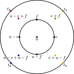
P¯¯𝑃\displaystyle\bar{P} supθ[0,2π)18[4+2|cos(θ2)|+2|sin(θ2)|]=12(1+12)absentsubscriptsupremum𝜃02𝜋18delimited-[]42𝜃22𝜃212112\displaystyle\leq\sup_{\theta\in[0,2\pi)}\frac{1}{8}\left[4+2\left|\cos\left(\frac{\theta}{2}\right)\right|+2\left|\sin\left(\frac{\theta}{2}\right)\right|\right]=\frac{1}{2}\left(1+\frac{1}{\sqrt{2}}\right)
Refer to caption
Figure 3. The optimal effects e=e0𝑒subscript𝑒0e=e_{0}, f=eθ𝑓subscript𝑒𝜃f=e_{\theta} and states t1=sφ1subscript𝑡1subscript𝑠subscript𝜑1t_{1}=s_{\varphi_{1}}, t2=sφ2subscript𝑡2subscript𝑠subscript𝜑2t_{2}=s_{\varphi_{2}}, t3=sφ3subscript𝑡3subscript𝑠subscript𝜑3t_{3}=s_{\varphi_{3}}, t4=sφ4subscript𝑡4subscript𝑠subscript𝜑4t_{4}=s_{\varphi_{4}} with θ=π/2𝜃𝜋2\theta=\pi/2, φ1=π/4subscript𝜑1𝜋4\varphi_{1}=\pi/4, φ2=3π/4subscript𝜑23𝜋4\varphi_{2}=3\pi/4, φ3=5π/4subscript𝜑35𝜋4\varphi_{3}=5\pi/4 and φ4=7π/4subscript𝜑47𝜋4\varphi_{4}=7\pi/4 for the maximal success probability (Eq. (15)) for the random access test in a rebit system as viewed from the positive z𝑧z-axis.

Furthermore, one can check that this bound is obtained with the following parameters: θ=π/2𝜃𝜋2\theta=\pi/2, φ1=π/4subscript𝜑1𝜋4\varphi_{1}=\pi/4, φ2=3π/4subscript𝜑23𝜋4\varphi_{2}=3\pi/4, φ3=5π/4subscript𝜑35𝜋4\varphi_{3}=5\pi/4 and φ4=7π/4subscript𝜑47𝜋4\varphi_{4}=7\pi/4. Thus, the optimal success probability of the random access test in rebit coincides with the corresponding optimal success probability in qubit. The optimal effects and states (up to rotational symmetry) are depicted in Fig. 3. We note that the optimal extreme effect f𝑓f aligns itself furthest away from both e𝑒e and ue𝑢𝑒u-e along the semicircle between them (this is because we are optimizing both e+f𝑒𝑓e+f and ue+f𝑢𝑒𝑓u-e+f at the same time) and the optimal states are uniquely determined by the sums e+f𝑒𝑓e+f, ue+f𝑢𝑒𝑓u-e+f, e+uf𝑒𝑢𝑓e+u-f and ue+uf𝑢𝑒𝑢𝑓u-e+u-f along the same directions in the (x,y)𝑥𝑦(x,y)-projection as is seen in Fig. 3.

7.3.2. Maximum success probability for polygons

Based on the rebit system we can compare the behaviour of the maximal success probability of RATs on polygons. In many ways polygons can be thought as discretized versions of the rebit system and depending on the coarseness of the discretization the studied properties may look a bit different or similar to the properties of the rebit. This is also the case with the optimal success probability of the random access test.
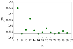
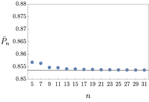
Refer to caption
Refer to caption
Figure 4. The maximum success probability P¯nsubscript¯𝑃𝑛\bar{P}_{n} of the random access test with two dichotomic measurements on even (above, green dots) and odd (below, blue dots) polygons as a function of the number of vertices n𝑛n of the polygon. The constant grey line is the maximum success probability of qubit (and rebit). From the even polygons we have excluded the case n=4𝑛4n=4 when P¯n=1subscript¯𝑃𝑛1\bar{P}_{n}=1.

As was established before, the maximum success probability for two dichotomic measurements on a regular polygon state space 𝒮nsubscript𝒮𝑛\mathcal{S}_{n}, denoted by P¯nsubscript¯𝑃𝑛\bar{P}_{n}, is maximized for some nontrivial extreme effects e,fext(𝒮n)𝑒𝑓superscript𝑒𝑥𝑡subscript𝒮𝑛e,f\in\mathcal{E}^{ext}(\mathcal{S}_{n}) and pure states t1,t2,t3,t4𝒮nextsubscript𝑡1subscript𝑡2subscript𝑡3subscript𝑡4subscriptsuperscript𝒮𝑒𝑥𝑡𝑛t_{1},t_{2},t_{3},t_{4}\in\mathcal{S}^{ext}_{n}. Because ext(𝒮n)={o,u,e1,,en}superscript𝑒𝑥𝑡subscript𝒮𝑛𝑜𝑢subscript𝑒1subscript𝑒𝑛\mathcal{E}^{ext}(\mathcal{S}_{n})=\{o,u,e_{1},\ldots,e_{n}\} when n𝑛n is even and ext(𝒮n)={o,u,g1,,gn,f1,,fn}superscript𝑒𝑥𝑡subscript𝒮𝑛𝑜𝑢subscript𝑔1subscript𝑔𝑛subscript𝑓1subscript𝑓𝑛\mathcal{E}^{ext}(\mathcal{S}_{n})=\{o,u,g_{1},\ldots,g_{n},f_{1},\ldots,f_{n}\} when n𝑛n is odd, so that ext(𝒮n)superscript𝑒𝑥𝑡subscript𝒮𝑛\mathcal{E}^{ext}(\mathcal{S}_{n}) (and 𝒮nextsubscriptsuperscript𝒮𝑒𝑥𝑡𝑛\mathcal{S}^{ext}_{n}) is finite in both cases, it is easy to calculate the maximum value for P¯nsubscript¯𝑃𝑛\bar{P}_{n} in the case of two dichotomic measurements for small values of n𝑛n. The results are shown in Fig. 4 for polygons with up to 303030 vertices.

From Fig. 4 we observe at least three interesting points. First, the maximum success probability is at least as high as that of the qubit (and the rebit) in every polygon state space, and in many of them it is higher. Second, as one would expect, in both cases P¯nsubscript¯𝑃𝑛\bar{P}_{n} seems to approach the maximum success probability of the qubit (and the rebit) as the number of vertices increase and the polygon starts to approximate the rebit system more closely geometrically. Third, the behaviour of P¯nsubscript¯𝑃𝑛\bar{P}_{n} is drastically different for even and odd n𝑛n: for even n𝑛n the maximum success probability P¯nsubscript¯𝑃𝑛\bar{P}_{n} seems to oscillate with decreasing amplitude whereas for odd n𝑛n it seems that P¯nsubscript¯𝑃𝑛\bar{P}_{n} approaches the qubit limit more monotonically. In the following we will analyse the results of Fig. 4 further by taking a closer look on the optimizing effects and states. We provide formulas for P¯nsubscript¯𝑃𝑛\bar{P}_{n} in every n𝑛n.

7.3.3. Optimality results for the maximum success probability in the even polygons

We will now look more closely on explaining Fig. 4 for even polygons. We will prove that the maximum success probability P¯nsubscript¯𝑃𝑛\bar{P}_{n} for two dichotomic measurements on even polygon state space 𝒮nsubscript𝒮𝑛\mathcal{S}_{n} depends on n𝑛n as follows:

P¯n=12(1+sec(πn)2)n=4m for odd msubscript¯𝑃𝑛121𝜋𝑛2n=4m for odd m\displaystyle\bar{P}_{n}=\frac{1}{2}\left(1+\frac{\sec\left(\frac{\pi}{n}\right)}{\sqrt{2}}\right)\quad\textrm{$n=4m$ for odd $m\in\mathbb{N}$ } (16)
P¯n=12(1+12)n=4m for even msubscript¯𝑃𝑛12112n=4m for even m\displaystyle\bar{P}_{n}=\frac{1}{2}\left(1+\frac{1}{\sqrt{2}}\right)\quad\textrm{$n=4m$ for even $m\in\mathbb{N}$} (17)
P¯n=14[2+rn2cos(mπn)+sin(mπn)]n=4m+2 for odd msubscript¯𝑃𝑛14delimited-[]2superscriptsubscript𝑟𝑛2𝑚𝜋𝑛𝑚𝜋𝑛n=4m+2 for odd m\displaystyle\bar{P}_{n}=\frac{1}{4}\left[2+r_{n}^{2}\cos\left(\frac{m\pi}{n}\right)+\sin\left(\frac{m\pi}{n}\right)\right]\quad\textrm{$n=4m+2$ for odd $m\in\mathbb{N}$} (18)
P¯n=14[2+cos(mπn)+rn2sin(mπn)]n=4m+2 for even msubscript¯𝑃𝑛14delimited-[]2𝑚𝜋𝑛superscriptsubscript𝑟𝑛2𝑚𝜋𝑛n=4m+2 for even m\displaystyle\bar{P}_{n}=\frac{1}{4}\left[2+\cos\left(\frac{m\pi}{n}\right)+r_{n}^{2}\sin\left(\frac{m\pi}{n}\right)\right]\quad\textrm{$n=4m+2$ for even $m\in\mathbb{N}$} (19)

(In the last two expressions rn=sec(πn)subscript𝑟𝑛𝜋𝑛r_{n}=\sqrt{\sec\left(\frac{\pi}{n}\right)} as before.) Thus, we will see that in the cases when n=4m+2𝑛4𝑚2n=4m+2, where m𝑚m is odd or even, or n=4m𝑛4𝑚n=4m, where m𝑚m is even, the maximum success probability is strictly larger than that of the qubit and the rebit, whereas for n=4m𝑛4𝑚n=4m, where m𝑚m is even, it is exactly the same as in qubit. In all cases the limit n𝑛n\to\infty matches the qubit value.

We start by deriving an upper for the maximum success probability P¯nsubscript¯𝑃𝑛\bar{P}_{n} similarly to how we did in the case of rebit. Let us consider the RAT for two dichotomic measurements as stated in Eq. (15). The polygons are symmetrical in the sense that we can fix the first extreme effect e𝑒e to be any of the nontrivial extreme effects and for even polygons we choose e=e1𝑒subscript𝑒1e=e_{1}. Furthermore, we have that f=ek𝑓subscript𝑒𝑘f=e_{k} for some k{1,,n}𝑘1𝑛k\in\{1,\ldots,n\} and ti=sjisubscript𝑡𝑖subscript𝑠subscript𝑗𝑖t_{i}=s_{j_{i}} for some ji{1,,n}subscript𝑗𝑖1𝑛j_{i}\in\{1,\ldots,n\} for all i{1,2,3,4}𝑖1234i\in\{1,2,3,4\}. With this notation we can write P¯nsubscript¯𝑃𝑛\bar{P}_{n} for even polygons as

P¯n=supk{1,,n}18[supj1{1,,n}(e1+ek)(sj1)+supj2{1,,n}(ue1+ek)(sj2)+supj3{1,,n}(ue1+uek)(sj3)+supj4{1,,n}(e1+uek)(sj4)].subscript¯𝑃𝑛subscriptsupremum𝑘1𝑛18subscriptsupremumsubscript𝑗11𝑛subscript𝑒1subscript𝑒𝑘subscript𝑠subscript𝑗1subscriptsupremumsubscript𝑗21𝑛𝑢subscript𝑒1subscript𝑒𝑘subscript𝑠subscript𝑗2subscriptsupremumsubscript𝑗31𝑛𝑢subscript𝑒1𝑢subscript𝑒𝑘subscript𝑠subscript𝑗3subscriptsupremumsubscript𝑗41𝑛subscript𝑒1𝑢subscript𝑒𝑘subscript𝑠subscript𝑗4\displaystyle\begin{split}\bar{P}_{n}&=\sup_{k\in\{1,\ldots,n\}}\frac{1}{8}\left[\sup_{j_{1}\in\{1,\ldots,n\}}(e_{1}+e_{k})(s_{j_{1}})+\sup_{j_{2}\in\{1,\ldots,n\}}(u-e_{1}+e_{k})(s_{j_{2}})\right.\\ &\ \ \ \left.+\sup_{j_{3}\in\{1,\ldots,n\}}(u-e_{1}+u-e_{k})(s_{j_{3}})+\sup_{j_{4}\in\{1,\ldots,n\}}(e_{1}+u-e_{k})(s_{j_{4}})\right].\end{split} (20)

First we note that we can restrict k{1,,n/2}𝑘1𝑛2k\in\{1,\ldots,n/2\} since otherwise we can just take f=uek=ek+n/2𝑓𝑢subscript𝑒𝑘subscript𝑒𝑘𝑛2f=u-e_{k}=e_{k+n/2} instead of f=ek𝑓subscript𝑒𝑘f=e_{k}. By expanding the previous expression and by using some trigonometric identities we can rewrite the previous equation as

P¯nsubscript¯𝑃𝑛\displaystyle\bar{P}_{n} =supk{1,,n/2}18[supj1{1,,n}(1+rn2cos((k1)πn)cos((k2j1)πn))\displaystyle=\sup_{k\in\{1,\ldots,n/2\}}\frac{1}{8}\left[\sup_{j_{1}\in\{1,\ldots,n\}}\left(1+r_{n}^{2}\cos\left(\frac{(k-1)\pi}{n}\right)\cos\left(\frac{(k-2j_{1})\pi}{n}\right)\right)\right.
+supj2{1,,n}(1rn2sin((k1)πn)sin((k2j2)πn))subscriptsupremumsubscript𝑗21𝑛1superscriptsubscript𝑟𝑛2𝑘1𝜋𝑛𝑘2subscript𝑗2𝜋𝑛\displaystyle\quad\quad\quad\quad\quad\ \ +\sup_{j_{2}\in\{1,\ldots,n\}}\left(1-r_{n}^{2}\sin\left(\frac{(k-1)\pi}{n}\right)\sin\left(\frac{(k-2j_{2})\pi}{n}\right)\right)
+supj3{1,,n}(1rn2cos((k1)πn)cos((k2j3)πn))subscriptsupremumsubscript𝑗31𝑛1superscriptsubscript𝑟𝑛2𝑘1𝜋𝑛𝑘2subscript𝑗3𝜋𝑛\displaystyle\quad\quad\quad\quad\quad\ \ +\sup_{j_{3}\in\{1,\ldots,n\}}\left(1-r_{n}^{2}\cos\left(\frac{(k-1)\pi}{n}\right)\cos\left(\frac{(k-2j_{3})\pi}{n}\right)\right)
+supj4{1,,n}(1+rn2sin((k1)πn)sin((k2j4)πn))].\displaystyle\left.\quad\quad\quad\quad\quad\ \ +\sup_{j_{4}\in\{1,\ldots,n\}}\left(1+r_{n}^{2}\sin\left(\frac{(k-1)\pi}{n}\right)\sin\left(\frac{(k-2j_{4})\pi}{n}\right)\right)\right].

Analogously to the rebit, we can upper bound the inner supremums by the terms 1+rn2|cos((k1)π/n)|1superscriptsubscript𝑟𝑛2𝑘1𝜋𝑛1+r_{n}^{2}|\cos((k-1)\pi/n)| and 1+rn2|sin((k1)π/n)|1superscriptsubscript𝑟𝑛2𝑘1𝜋𝑛1+r_{n}^{2}|\sin((k-1)\pi/n)| from which we can omit the absolute values since cos((k1)π/n)0𝑘1𝜋𝑛0\cos((k-1)\pi/n)\geq 0 and sin((k1)π/n)0𝑘1𝜋𝑛0\sin((k-1)\pi/n)\geq 0 for all k{1,,n/2}𝑘1𝑛2k\in\{1,\ldots,n/2\}. For the remaining (outer) supremum we can use the upper bound cos((k1)π/n)+sin((k1)π/n)2𝑘1𝜋𝑛𝑘1𝜋𝑛2\cos((k-1)\pi/n)+\sin((k-1)\pi/n)\leq\sqrt{2} so that in the end we get the following upper bound for P¯nsubscript¯𝑃𝑛\bar{P}_{n} for all even polygons:

P¯nsubscript¯𝑃𝑛\displaystyle\bar{P}_{n} supk{1,,n/2}18[4+2rn2cos((k1)πn)+2rn2sin((k1)πn)]absentsubscriptsupremum𝑘1𝑛218delimited-[]42superscriptsubscript𝑟𝑛2𝑘1𝜋𝑛2superscriptsubscript𝑟𝑛2𝑘1𝜋𝑛\displaystyle\leq\sup_{k\in\{1,\ldots,n/2\}}\frac{1}{8}\left[4+2r_{n}^{2}\cos\left(\frac{(k-1)\pi}{n}\right)+2r_{n}^{2}\sin\left(\frac{(k-1)\pi}{n}\right)\right]
12(1+rn22)=12(1+sec(πn)2).absent121superscriptsubscript𝑟𝑛22121𝜋𝑛2\displaystyle\leq\frac{1}{2}\left(1+\frac{r_{n}^{2}}{\sqrt{2}}\right)=\frac{1}{2}\left(1+\frac{\sec\left(\frac{\pi}{n}\right)}{\sqrt{2}}\right). (21)

One can confirm that the above bound is attained when we take k=1+n/4𝑘1𝑛4k=1+n/4, j1=k/2subscript𝑗1𝑘2j_{1}=k/2, j2=k/2+n/4subscript𝑗2𝑘2𝑛4j_{2}=k/2+n/4, j3=k/2+n/2subscript𝑗3𝑘2𝑛2j_{3}=k/2+n/2 and j4=k/2+3n/4subscript𝑗4𝑘23𝑛4j_{4}=k/2+3n/4. However, since k,j1,j2,j3,j4𝑘subscript𝑗1subscript𝑗2subscript𝑗3subscript𝑗4k,j_{1},j_{2},j_{3},j_{4} must be integers, this upper bound can be attained only in the case when n=4m𝑛4𝑚n=4m for some m𝑚m\in\mathbb{N} (so that k𝑘k is an integer) and m𝑚m is odd (so that k=1+m𝑘1𝑚k=1+m is even and j1,j2,j3,j4subscript𝑗1subscript𝑗2subscript𝑗3subscript𝑗4j_{1},j_{2},j_{3},j_{4} are integers). Thus, in this case we have that f=em+1𝑓subscript𝑒𝑚1f=e_{m+1}, t1=sm+12subscript𝑡1subscript𝑠𝑚12t_{1}=s_{\frac{m+1}{2}}, t2=s3m+12subscript𝑡2subscript𝑠3𝑚12t_{2}=s_{\frac{3m+1}{2}}, t3=s5m+12subscript𝑡3subscript𝑠5𝑚12t_{3}=s_{\frac{5m+1}{2}} and t4=s7m+12subscript𝑡4subscript𝑠7𝑚12t_{4}=s_{\frac{7m+1}{2}}.

From the previous result it becomes immediate that we must consider different cases also within the even polygons. Let us next consider the case when n=4m𝑛4𝑚n=4m but m𝑚m is even. As we saw above, we cannot saturate the previous bound for P¯nsubscript¯𝑃𝑛\bar{P}_{n} in this case because in this case the optimizing values for jisubscript𝑗𝑖j_{i}’s are not integers. However, the expressions for the inner supremums which we are upper bounding, namely cos((k2j1)π/n)𝑘2subscript𝑗1𝜋𝑛\cos((k-2j_{1})\pi/n), sin((k2j2)π/n)𝑘2subscript𝑗2𝜋𝑛-\sin((k-2j_{2})\pi/n), sin((k2j3)π/n)𝑘2subscript𝑗3𝜋𝑛\sin((k-2j_{3})\pi/n) and cos((k2j4)π/n)𝑘2subscript𝑗4𝜋𝑛-\cos((k-2j_{4})\pi/n), are discrete and of simple form so that we know that even if we cannot attain the optimal value 111 for these expressions with the optimal parameters, the actual supremums are attained with parameters close to the the ones presented above.

Let us consider separately two different cases when n=4m𝑛4𝑚n=4m and m𝑚m is even. First, let us consider the case that k𝑘k is even so that the optimal values for jisubscript𝑗𝑖j_{i}’s are integers and the first inequality in Eq. (21) is saturated, i.e., the inner supremums have the same optimal values as above. Again, in this case they are either of the form 1+rn2cos((k1)π/n)1superscriptsubscript𝑟𝑛2𝑘1𝜋𝑛1+r_{n}^{2}\cos((k-1)\pi/n) or 1+rn2sin((k1)π/n)1superscriptsubscript𝑟𝑛2𝑘1𝜋𝑛1+r_{n}^{2}\sin((k-1)\pi/n) and they are attained with j1=k/2subscript𝑗1𝑘2j_{1}=k/2, j2=k/2+msubscript𝑗2𝑘2𝑚j_{2}=k/2+m, j3=k/2+2msubscript𝑗3𝑘22𝑚j_{3}=k/2+2m and j4=k/2+3msubscript𝑗4𝑘23𝑚j_{4}=k/2+3m. However, the second inequality is saturated, i.e., the outer supremum attains the previous optimal value, only when k=m+1𝑘𝑚1k=m+1 which would make k𝑘k odd since m𝑚m is even. Therefore we cannot attain the previous bound in this case. Instead, for the outer supremum we must maximize cos((k1)π/n)+sin((k1)π/n)𝑘1𝜋𝑛𝑘1𝜋𝑛\cos((k-1)\pi/n)+\sin((k-1)\pi/n) for all even values of k{1,,n/2}𝑘1𝑛2k\in\{1,\ldots,n/2\}. From the form of this expression we see that the supremum must be attained with the closest even integer value to m+1𝑚1m+1, i.e., either with k=m𝑘𝑚k=m or k=m+2𝑘𝑚2k=m+2. We can verify that then for both of these values of k𝑘k we have that cos((k1)π/n)+sin((k1)π/n)=2/rn2𝑘1𝜋𝑛𝑘1𝜋𝑛2superscriptsubscript𝑟𝑛2\cos((k-1)\pi/n)+\sin((k-1)\pi/n)=\sqrt{2}/r_{n}^{2} and hence P¯n(e,f)=1/2(1+1/2)subscript¯𝑃𝑛𝑒𝑓12112\bar{P}_{n}(e,f)=1/2(1+1/\sqrt{2}) with the optimizing states t1=sm2subscript𝑡1subscript𝑠𝑚2t_{1}=s_{\frac{m}{2}}, t2=s3m2subscript𝑡2subscript𝑠3𝑚2t_{2}=s_{\frac{3m}{2}}, t3=s5m2subscript𝑡3subscript𝑠5𝑚2t_{3}=s_{\frac{5m}{2}} and t4=s7m2subscript𝑡4subscript𝑠7𝑚2t_{4}=s_{\frac{7m}{2}} for the optimizing effect f=em𝑓subscript𝑒𝑚f=e_{m}, and t1=sm2+1subscript𝑡1subscript𝑠𝑚21t_{1}=s_{\frac{m}{2}+1}, t2=s3m2+1subscript𝑡2subscript𝑠3𝑚21t_{2}=s_{\frac{3m}{2}+1}, t3=s5m2+1subscript𝑡3subscript𝑠5𝑚21t_{3}=s_{\frac{5m}{2}+1} and t4=s7m2+1subscript𝑡4subscript𝑠7𝑚21t_{4}=s_{\frac{7m}{2}+1} for the optimizing effect f=em+2𝑓subscript𝑒𝑚2f=e_{m+2}.

Second, let us assume that k𝑘k is odd so that the first inequality in Eq. (21) is not saturated, i.e., that the previously presented optimal values for jisubscript𝑗𝑖j_{i}’s are not integers. In this case the actual optimizing values for the inner supremums must then be the closest integers to the values considered before. Thus, the inner supremums must be attained with the following values: j±1=(k±1)/2subscript𝑗plus-or-minus1plus-or-minus𝑘12j_{\pm 1}=(k\pm 1)/2, j±2=(k±1)/2+msubscript𝑗plus-or-minus2plus-or-minus𝑘12𝑚j_{\pm 2}=(k\pm 1)/2+m, j±3=(k±1)/2+2msubscript𝑗plus-or-minus3plus-or-minus𝑘122𝑚j_{\pm 3}=(k\pm 1)/2+2m and j±4=(k±1)/2+3msubscript𝑗plus-or-minus4plus-or-minus𝑘123𝑚j_{\pm 4}=(k\pm 1)/2+3m. It is straightforward to verify that in both cases, i.e., when one uses either j+isubscript𝑗𝑖j_{+i}’s or jisubscript𝑗𝑖j_{-i}’s, the inner supremums take the values 1+cos((k1)π/n)1𝑘1𝜋𝑛1+\cos((k-1)\pi/n) or 1+sin((k1)π/n)1𝑘1𝜋𝑛1+\sin((k-1)\pi/n) depending on which expression we are evaluating. Now the outer supermum can attain the same optimal value as before with the parameter value k=m+1𝑘𝑚1k=m+1 (which is odd because m𝑚m is even). Finally we obtain that also in this case P¯n(e,f)=1/2(1+1/2)subscript¯𝑃𝑛𝑒𝑓12112\bar{P}_{n}(e,f)=1/2(1+1/\sqrt{2}) with the effect f=em+1𝑓subscript𝑒𝑚1f=e_{m+1} and optimizing states t1=sm2subscript𝑡1subscript𝑠𝑚2t_{1}=s_{\frac{m}{2}} or t1=sm2+1subscript𝑡1subscript𝑠𝑚21t_{1}=s_{\frac{m}{2}+1}, t2=s3m2subscript𝑡2subscript𝑠3𝑚2t_{2}=s_{\frac{3m}{2}} or t2=s3m2+1subscript𝑡2subscript𝑠3𝑚21t_{2}=s_{\frac{3m}{2}+1}, t3=s5m2subscript𝑡3subscript𝑠5𝑚2t_{3}=s_{\frac{5m}{2}} or t3=s5m2+1subscript𝑡3subscript𝑠5𝑚21t_{3}=s_{\frac{5m}{2}+1} and t4=s7m2subscript𝑡4subscript𝑠7𝑚2t_{4}=s_{\frac{7m}{2}} or t4=s7m2+1subscript𝑡4subscript𝑠7𝑚21t_{4}=s_{\frac{7m}{2}+1}.

To conclude, we have shown that the maximum success probability for an even polygon with n=4m𝑛4𝑚n=4m for some m𝑚m\in\mathbb{N} are given by Eqs. (16) and (17). All the optimal effects and states are explicitly expressed in Table 1.

n𝑛n 4m4𝑚4m
m𝑚m odd even
e𝑒e e1subscript𝑒1e_{1} e1subscript𝑒1e_{1}
f𝑓f em+1subscript𝑒𝑚1e_{m+1} emsubscript𝑒𝑚e_{m} em+1subscript𝑒𝑚1e_{m+1} em+2subscript𝑒𝑚2e_{m+2}
t1subscript𝑡1t_{1} sm+12subscript𝑠𝑚12s_{\frac{m+1}{2}} sm2subscript𝑠𝑚2s_{\frac{m}{2}} sm+1±12subscript𝑠plus-or-minus𝑚112s_{\frac{m+1\pm 1}{2}} sm2+1subscript𝑠𝑚21s_{\frac{m}{2}+1}
t2subscript𝑡2t_{2} s3m+12subscript𝑠3𝑚12s_{\frac{3m+1}{2}} s3m2subscript𝑠3𝑚2s_{\frac{3m}{2}} s3m+1±12subscript𝑠plus-or-minus3𝑚112s_{\frac{3m+1\pm 1}{2}} s3m2+1subscript𝑠3𝑚21s_{\frac{3m}{2}+1}
t3subscript𝑡3t_{3} s5m+12subscript𝑠5𝑚12s_{\frac{5m+1}{2}} s5m2subscript𝑠5𝑚2s_{\frac{5m}{2}} s5m+1±12subscript𝑠plus-or-minus5𝑚112s_{\frac{5m+1\pm 1}{2}} s5m2+1subscript𝑠5𝑚21s_{\frac{5m}{2}+1}
t4subscript𝑡4t_{4} s7m+12subscript𝑠7𝑚12s_{\frac{7m+1}{2}} s7m2subscript𝑠7𝑚2s_{\frac{7m}{2}} s7m+1±12subscript𝑠plus-or-minus7𝑚112s_{\frac{7m+1\pm 1}{2}} s7m2+1subscript𝑠7𝑚21s_{\frac{7m}{2}+1}
P¯nsubscript¯𝑃𝑛\bar{P}_{n} 12(1+rn22)121superscriptsubscript𝑟𝑛22\frac{1}{2}\left(1+\frac{r_{n}^{2}}{\sqrt{2}}\right) 12(1+12)12112\frac{1}{2}\left(1+\frac{1}{\sqrt{2}}\right)
Table 1. The optimal effects and states for the random access test with two dichotomic measurements on even polygon state spaces 𝒮nsubscript𝒮𝑛\mathcal{S}_{n}, where n=4m𝑛4𝑚n=4m for some m𝑚m\in\mathbb{N}. When m𝑚m is even, the optimizing effect f𝑓f is not unique and thus also the optimizing states are different for different choises of f𝑓f and furthermore they may not be unique even for a fixed choice of f𝑓f.

Let us then consider the case when n4m𝑛4𝑚n\neq 4m for any m𝑚m\in\mathbb{N} so that we must actually then have that n=4m+2𝑛4𝑚2n=4m+2 for some m𝑚m\in\mathbb{N}. In this case we can again distinguish two different cases: when m𝑚m is odd and when m𝑚m is even. To see the reason for this, let us consider the expression for P¯nsubscript¯𝑃𝑛\bar{P}_{n} when n=4m+2𝑛4𝑚2n=4m+2. In this case we see that the maximum possible value for the inner supremums can be attained if j1=k/2subscript𝑗1𝑘2j_{1}=k/2, j2=k/2+m+1/2subscript𝑗2𝑘2𝑚12j_{2}=k/2+m+1/2, j3=k/2+2msubscript𝑗3𝑘22𝑚j_{3}=k/2+2m and j4=k/2+3m+3/2subscript𝑗4𝑘23𝑚32j_{4}=k/2+3m+3/2. However, we see that these are not integers neither for odd or even k𝑘k.

If we assume that k𝑘k is even, then the closest integers with which we can attain the supremum are j1=k/2subscriptsuperscript𝑗1𝑘2j^{\prime}_{1}=k/2, j±2=(k±1)/2+m+1/2subscriptsuperscript𝑗plus-or-minus2plus-or-minus𝑘12𝑚12j^{\prime}_{\pm 2}=(k\pm 1)/2+m+1/2, j3=k/2+2msubscriptsuperscript𝑗3𝑘22𝑚j^{\prime}_{3}=k/2+2m and j±4=(k±1)/2+3m+3/2subscriptsuperscript𝑗plus-or-minus4plus-or-minus𝑘123𝑚32j^{\prime}_{\pm 4}=(k\pm 1)/2+3m+3/2. For these parameters we get that

P¯nsubscript¯𝑃𝑛\displaystyle\bar{P}_{n} =supk{1,,n/2}18[4+2rn2cos((k1)πn)+2sin((k1)πn)]absentsubscriptsupremum𝑘1𝑛218delimited-[]42superscriptsubscript𝑟𝑛2𝑘1𝜋𝑛2𝑘1𝜋𝑛\displaystyle=\sup_{k\in\{1,\ldots,n/2\}}\frac{1}{8}\left[4+2r_{n}^{2}\cos\left(\frac{(k-1)\pi}{n}\right)+2\sin\left(\frac{(k-1)\pi}{n}\right)\right]

It can be shown that in this case the optimizing value for k𝑘k can be restricted to be either m+1𝑚1m+1 or m+2𝑚2m+2. Since we are assuming that k𝑘k is even, this leads to two different considerations: when m𝑚m is even and when m𝑚m is odd. For odd m𝑚m we have that the optimal value is k=m+1𝑘𝑚1k=m+1 and in this case Eq. (18) holds. Similarly for even m𝑚m we have that the optimal value is k=m+2𝑘𝑚2k=m+2 and in this case Eq. (19) holds.

On the other hand, if we assume that k𝑘k is odd, then the optimizing values for jisubscript𝑗𝑖j_{i}’s are j±1′′=(k±1)/2subscriptsuperscript𝑗′′plus-or-minus1plus-or-minus𝑘12j^{\prime\prime}_{\pm 1}=(k\pm 1)/2, j2′′=k/2+m+1/2subscriptsuperscript𝑗′′2𝑘2𝑚12j^{\prime\prime}_{2}=k/2+m+1/2, j±3′′=(k±1)/2+2msubscriptsuperscript𝑗′′plus-or-minus3plus-or-minus𝑘122𝑚j^{\prime\prime}_{\pm 3}=(k\pm 1)/2+2m and j4′′=k/2+3m+3/2subscriptsuperscript𝑗′′4𝑘23𝑚32j^{\prime\prime}_{4}=k/2+3m+3/2. For these parameters we get that

P¯nsubscript¯𝑃𝑛\displaystyle\bar{P}_{n} =supk{1,,n/2}18[4+2cos((k1)πn)+2rn2sin((k1)πn)]absentsubscriptsupremum𝑘1𝑛218delimited-[]42𝑘1𝜋𝑛2superscriptsubscript𝑟𝑛2𝑘1𝜋𝑛\displaystyle=\sup_{k\in\{1,\ldots,n/2\}}\frac{1}{8}\left[4+2\cos\left(\frac{(k-1)\pi}{n}\right)+2r_{n}^{2}\sin\left(\frac{(k-1)\pi}{n}\right)\right]

Also in this case the optimizing value for k𝑘k can be shown to be either m+1𝑚1m+1 or m+2𝑚2m+2. Again we have different cases for even and odd m𝑚m. For odd m𝑚m we have that the optimal value is k=m+2𝑘𝑚2k=m+2 and then one can confirm that we get Eq. (18). Similarly for even m𝑚m we have that the optimal value is k=m+1𝑘𝑚1k=m+1 and then one can confirm that we get Eq. (19).

To conclude, the maximum success probabilities in the case n=4m+2𝑛4𝑚2n=4m+2 are given by Eq. (18) when m𝑚m is odd and by Eq. (19) when m𝑚m is even. One can show that both of these expressions are strictly between the qubit (and the rebit) value 1/2(1+1/2)121121/2(1+1/\sqrt{2}) and the upper bound given in Eq. (21) for all finite m𝑚m\in\mathbb{N}. In the limit m𝑚m\to\infty the maximum success probability approaches the qubit value. All the optimal effects and states are explicitly expressed in Table 2.

n𝑛n 4m+24𝑚24m+2
m𝑚m odd even
e𝑒e e1subscript𝑒1e_{1} e1subscript𝑒1e_{1}
f𝑓f em+1subscript𝑒𝑚1e_{m+1} em+2subscript𝑒𝑚2e_{m+2} em+1subscript𝑒𝑚1e_{m+1} em+2subscript𝑒𝑚2e_{m+2}
t1subscript𝑡1t_{1} sm+12subscript𝑠𝑚12s_{\frac{m+1}{2}} sm±12+1subscript𝑠plus-or-minus𝑚121s_{\frac{m\pm 1}{2}+1} sm+1±12subscript𝑠plus-or-minus𝑚112s_{\frac{m+1\pm 1}{2}} sm2+1subscript𝑠𝑚21s_{\frac{m}{2}+1}
t2subscript𝑡2t_{2} s3m±12+1subscript𝑠plus-or-minus3𝑚121s_{\frac{3m\pm 1}{2}+1} s3m+12+1subscript𝑠3𝑚121s_{\frac{3m+1}{2}+1} s3m2+1subscript𝑠3𝑚21s_{\frac{3m}{2}+1} s3m+1±12+1subscript𝑠plus-or-minus3𝑚1121s_{\frac{3m+1\pm 1}{2}+1}
t3subscript𝑡3t_{3} s5m+12+1subscript𝑠5𝑚121s_{\frac{5m+1}{2}+1} s5m±12+2subscript𝑠plus-or-minus5𝑚122s_{\frac{5m\pm 1}{2}+2} s5m+1±12+1subscript𝑠plus-or-minus5𝑚1121s_{\frac{5m+1\pm 1}{2}+1} s5m2+2subscript𝑠5𝑚22s_{\frac{5m}{2}+2}
t4subscript𝑡4t_{4} s7m±12+2subscript𝑠plus-or-minus7𝑚122s_{\frac{7m\pm 1}{2}+2} s7m+12+2subscript𝑠7𝑚122s_{\frac{7m+1}{2}+2} s7m2+2subscript𝑠7𝑚22s_{\frac{7m}{2}+2} s7m+1±12+2subscript𝑠plus-or-minus7𝑚1122s_{\frac{7m+1\pm 1}{2}+2}
P¯nsubscript¯𝑃𝑛\bar{P}_{n} 14[2+rn2cos(mπn)+sin(mπn)]14delimited-[]2superscriptsubscript𝑟𝑛2𝑚𝜋𝑛𝑚𝜋𝑛\frac{1}{4}\left[2+r_{n}^{2}\cos\left(\frac{m\pi}{n}\right)+\sin\left(\frac{m\pi}{n}\right)\right] 14[2+cos(mπn)+rn2sin(mπn)]14delimited-[]2𝑚𝜋𝑛superscriptsubscript𝑟𝑛2𝑚𝜋𝑛\frac{1}{4}\left[2+\cos\left(\frac{m\pi}{n}\right)+r_{n}^{2}\sin\left(\frac{m\pi}{n}\right)\right]
Table 2. The optimal effects and states for the random access test with two dichotomic measurements on even polygon state spaces 𝒮nsubscript𝒮𝑛\mathcal{S}_{n}, where n=4m+2𝑛4𝑚2n=4m+2 for some m𝑚m\in\mathbb{N}. For both even and odd m𝑚m the optimizing effect f𝑓f is not unique and thus also the optimizing states are different for different choices of f𝑓f and furthermore they may not be unique even for a fixed choice of f𝑓f.

7.3.4. Comparing rebit to the even polygon state spaces

As was established in the previous section, instead of having a single oscillatory upper bound that would explain the behaviour of the maximum success probability depicted in Fig. 4 we must in fact divide the even polygons in four distinct cases: i) n=4m𝑛4𝑚n=4m and m𝑚m is odd, ii) n=4m𝑛4𝑚n=4m and m𝑚m is even, iii) n=4m+2𝑛4𝑚2n=4m+2 and m𝑚m is odd, and iv) n=4m+2𝑛4𝑚2n=4m+2 and m𝑚m is even for some m𝑚m\in\mathbb{N}.

Refer to caption
Refer to caption
Refer to caption
Refer to caption
Figure 5. Some of the maximizing effects and states for the first four even polygons. The sums of the maximizing effects and their maximizing states are represented by the same colors as in Fig. 3. For comparison, the optimal effects and states in rebit are denoted in gray.

Regarding the geometry of the optimal effects and the states, as was explained previously, we can freely choose e=e1𝑒subscript𝑒1e=e_{1}. According to our analysis, similarly to the rebit case, the second extreme effect f𝑓f is aligned so that it is ‘furthest’ away from both e𝑒e and ue𝑢𝑒u-e along the circumsphere of the polygon, i.e., taking values f=ek𝑓subscript𝑒𝑘f=e_{k} where k{m,m+1,m+2}𝑘𝑚𝑚1𝑚2k\in\{m,m+1,m+2\} depending on the polygon. Finally, again just as in the rebit, the optimizing states t1,t2,t3,t4subscript𝑡1subscript𝑡2subscript𝑡3subscript𝑡4t_{1},t_{2},t_{3},t_{4} are (not necessarily uniquely) determined by the sums e+f𝑒𝑓e+f, ue+f𝑢𝑒𝑓u-e+f, e+uf𝑒𝑢𝑓e+u-f and ue+uf𝑢𝑒𝑢𝑓u-e+u-f as close to the same directions of these sums in the 2-dimensional (x,y)𝑥𝑦(x,y)-projections as possible.

We illustrate the previous properties along with pointing out the differences of the four aforementioned cases by depicting some of the optimal effects and states in the first four even polygons in Fig. 5. We see the first two cases when n=4m𝑛4𝑚n=4m with m=1𝑚1m=1 and m=2𝑚2m=2 depicted on the left, whereas the first two cases when n=4m+2𝑛4𝑚2n=4m+2 with m=1𝑚1m=1 and m=2𝑚2m=2 depicted on the right. Furthermore, the top figures are examples of the cases when m𝑚m is odd and the bottom ones are examples of the cases when m𝑚m is even. The depicted states and effects are chosen from Tables 1 and 2 in such a that we take f=em+1𝑓subscript𝑒𝑚1f=e_{m+1} for all of the different cases and if there are more than one optimizing state for these optimizing effects, then we take the equal convex mixture of such states for the reasons explained below.

From the figure we see that in the cases when n=4m𝑛4𝑚n=4m the alignment of the optimal effects e𝑒e and f𝑓f can be chosen to be just as in the rebit state space. However, the alignment of the optimal states differ for odd and even m𝑚m: if m𝑚m is odd, then the optimal states t1,t2,t3,t4subscript𝑡1subscript𝑡2subscript𝑡3subscript𝑡4t_{1},t_{2},t_{3},t_{4} are unique pure states and aligned in the same direction in the (x,y)𝑥𝑦(x,y)-projection as the sums of the optimal effects (just as in the rebit), but in the case that m𝑚m is even, the optimal states are not unique and they can be chosen from the corresponding 2-dimensional faces of the state space. In particular, for illustration purposes, for even m𝑚m we chose the optimal states to be of the form ti=1/2(sji+sji+1)subscript𝑡𝑖12subscript𝑠subscript𝑗𝑖subscript𝑠subscript𝑗𝑖1t_{i}=1/2(s_{j_{i}}+s_{j_{i}+1}) for some ji{1,,n}subscript𝑗𝑖1𝑛j_{i}\in\{1,\ldots,n\} for all i{1,2,3,4}𝑖1234i\in\{1,2,3,4\} so that they align in the same direction as the sums of the optimal effects e𝑒e and f𝑓f in the 2-dimensional (x,y)𝑥𝑦(x,y)-projection just as in the case of odd m𝑚m and the rebit. However, in the case that n=4m+2𝑛4𝑚2n=4m+2 already for m=1𝑚1m=1 and m=2𝑚2m=2 the situation differs from that of the rebit and the qubit since the effect f𝑓f cannot be chosen to be orthogonal to e𝑒e in the (x,y)𝑥𝑦(x,y)-projection in the z=1/2𝑧12z=1/2–plane as before. For this reason also the optimal states are determined differently: after fixing the effects e=e1𝑒subscript𝑒1e=e_{1} and f=em+1𝑓subscript𝑒𝑚1f=e_{m+1}, for odd m𝑚m we have that t1subscript𝑡1t_{1} and t3subscript𝑡3t_{3} are uniquely determined and t2subscript𝑡2t_{2} and t4subscript𝑡4t_{4} are not (and we choose them along the same direction with the sums of the respective optimizing effects), whereas for even m𝑚m it is the opposite.

7.3.5. Odd polygons

In odd polygons theories the maximum success probability P¯nsubscript¯𝑃𝑛\bar{P}_{n} for two dichotomic measurements depends on n𝑛n as follows:

P¯n=14[2+cos(mπn)+r2n2sin(mπn)] n=4m+1 for msubscript¯𝑃𝑛14delimited-[]2𝑚𝜋𝑛superscriptsubscript𝑟2𝑛2𝑚𝜋𝑛 n=4m+1 for m\displaystyle\bar{P}_{n}=\frac{1}{4}\left[2+\cos\left(\tfrac{m\pi}{n}\right)+r_{2n}^{2}\sin\left(\tfrac{m\pi}{n}\right)\right]\quad\textrm{ $n=4m+1$ for $m\in\mathbb{N}$} (22)
P¯n=14[2+cos((m+1)πn)+r2n2sin((m+1)πn)] n=4m+3 for m,subscript¯𝑃𝑛14delimited-[]2𝑚1𝜋𝑛superscriptsubscript𝑟2𝑛2𝑚1𝜋𝑛 n=4m+3 for m\displaystyle\bar{P}_{n}=\frac{1}{4}\left[2+\cos\left(\tfrac{(m+1)\pi}{n}\right)+r_{2n}^{2}\sin\left(\tfrac{(m+1)\pi}{n}\right)\right]\ \textrm{ $n=4m+3$ for $m\in\mathbb{N}$}, (23)

where r2n=sec(π2n)subscript𝑟2𝑛𝜋2𝑛r_{2n}=\sqrt{\sec\left(\frac{\pi}{2n}\right)}.

The proof of these results is similar to our previous proof in case of the even polygon theories. In Eq. (15) we can fix the first extreme effect e𝑒e to be any of the nontrivial extreme effects and for odd polygons we choose e=g1𝑒subscript𝑔1e=g_{1}. Furthermore, we have that we can choose f=gk𝑓subscript𝑔𝑘f=g_{k} for some k{1,,n}𝑘1𝑛k\in\{1,\ldots,n\} and ti=sjisubscript𝑡𝑖subscript𝑠subscript𝑗𝑖t_{i}=s_{j_{i}} for some ji{1,,n}subscript𝑗𝑖1𝑛j_{i}\in\{1,\ldots,n\} for all i{1,2,3,4}𝑖1234i\in\{1,2,3,4\}. We can write P¯nsubscript¯𝑃𝑛\bar{P}_{n} for odd polygons as

P¯nsubscript¯𝑃𝑛\displaystyle\bar{P}_{n} =supk{1,,n}18[supj1{1,,n}(g1+gk)(sj1)+supj2{1,,n}(ug1+gk)(sj2)\displaystyle=\sup_{k\in\{1,\ldots,n\}}\frac{1}{8}\left[\sup_{j_{1}\in\{1,\ldots,n\}}(g_{1}+g_{k})(s_{j_{1}})+\sup_{j_{2}\in\{1,\ldots,n\}}(u-g_{1}+g_{k})(s_{j_{2}})\right.
+supj3{1,,n}(ug1+ugk)(sj3)+supj4{1,,n}(g1+ugk)(sj4)].\displaystyle\ \ \ \left.+\sup_{j_{3}\in\{1,\ldots,n\}}(u-g_{1}+u-g_{k})(s_{j_{3}})+\sup_{j_{4}\in\{1,\ldots,n\}}(g_{1}+u-g_{k})(s_{j_{4}})\right].

By expanding the previous expression and by using some trigonometric identities we can rewrite the previous equation as

P¯nsubscript¯𝑃𝑛\displaystyle\bar{P}_{n} =supk{1,,n}18[supj1{1,,n}11+rn2(2+2rn2cos((k1)πn)cos((k+12j1)πn))\displaystyle=\sup_{k\in\{1,\ldots,n\}}\frac{1}{8}\left[\sup_{j_{1}\in\{1,\ldots,n\}}\frac{1}{1+r_{n}^{2}}\left(2+2r_{n}^{2}\cos\left(\tfrac{(k-1)\pi}{n}\right)\cos\left(\tfrac{(k+1-2j_{1})\pi}{n}\right)\right)\right.
+supj2{1,,n}11+rn2(1+rn22rn2sin((k1)πn)sin((k+12j2)πn))subscriptsupremumsubscript𝑗21𝑛11superscriptsubscript𝑟𝑛21superscriptsubscript𝑟𝑛22superscriptsubscript𝑟𝑛2𝑘1𝜋𝑛𝑘12subscript𝑗2𝜋𝑛\displaystyle\quad\quad\ \ +\sup_{j_{2}\in\{1,\ldots,n\}}\frac{1}{1+r_{n}^{2}}\left(1+r_{n}^{2}-2r_{n}^{2}\sin\left(\tfrac{(k-1)\pi}{n}\right)\sin\left(\tfrac{(k+1-2j_{2})\pi}{n}\right)\right)
+supj3{1,,n}11+rn2(2rn22rn2cos((k1)πn)cos((k+12j3)πn))subscriptsupremumsubscript𝑗31𝑛11superscriptsubscript𝑟𝑛22superscriptsubscript𝑟𝑛22superscriptsubscript𝑟𝑛2𝑘1𝜋𝑛𝑘12subscript𝑗3𝜋𝑛\displaystyle\quad\quad\ \ +\sup_{j_{3}\in\{1,\ldots,n\}}\frac{1}{1+r_{n}^{2}}\left(2r_{n}^{2}-2r_{n}^{2}\cos\left(\tfrac{(k-1)\pi}{n}\right)\cos\left(\tfrac{(k+1-2j_{3})\pi}{n}\right)\right)
+supj4{1,,n}11+rn2(1+rn2+2rn2sin((k1)πn)sin((k+12j4)πn))].\displaystyle\left.\quad\quad\ \ +\sup_{j_{4}\in\{1,\ldots,n\}}\frac{1}{1+r_{n}^{2}}\left(1+r_{n}^{2}+2r_{n}^{2}\sin\left(\tfrac{(k-1)\pi}{n}\right)\sin\left(\tfrac{(k+1-2j_{4})\pi}{n}\right)\right)\right].

Similarly to as we did in the even polygons we can confirm that the algebraic maximum, and thus and upper bound for the actual maximum success probability, can be attained with parameters k=1+n/4𝑘1𝑛4k=1+n/4, j1=(k+1)/2subscript𝑗1𝑘12j_{1}=(k+1)/2, j2=(k+1)/2+n/4subscript𝑗2𝑘12𝑛4j_{2}=(k+1)/2+n/4, j3=(k+1)/2+n/2subscript𝑗3𝑘12𝑛2j_{3}=(k+1)/2+n/2 and j4=(k+1)/2+3n/4subscript𝑗4𝑘123𝑛4j_{4}=(k+1)/2+3n/4 in which case we have that

P¯n12(1+2rn21+rn2)=12(1+21+cos(πn)).subscript¯𝑃𝑛1212superscriptsubscript𝑟𝑛21superscriptsubscript𝑟𝑛212121𝜋𝑛\displaystyle\bar{P}_{n}\leq\frac{1}{2}\left(1+\frac{\sqrt{2}r_{n}^{2}}{1+r_{n}^{2}}\right)=\frac{1}{2}\left(1+\frac{\sqrt{2}}{1+\cos\left(\frac{\pi}{n}\right)}\right).

We note that for any finite n𝑛n this bound is always larger than the maximum success probability in qubit and in the limit n𝑛n\to\infty the bound coincides with the qubit value. However, unlike in the even polygon case, we cannot attain this upper bound in any odd polygon since k=1+n/4𝑘1𝑛4k=1+n/4 will never be an integer for odd n𝑛n. But since the optimized expressions are of the similar form as for even polygons we again know that the actual supremum values will be attained for parameter values close to those that attain the algebraic maximum. All the optimizing effects and states are presented in Table 3. We depict some of these optimal effects and states in Fig. 6 in similar fashion as we did in Fig. 5 for even polygons.
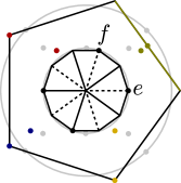
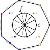
Refer to caption
Refer to caption
Refer to caption
Refer to caption
Figure 6. Some of the maximizing effects and states for the first four odd polygons. The sums of the maximizing effects and their maximizing states are represented by the same colors as in Fig. 3. For comparison, the optimal effects and states in rebit are denoted in gray.
n𝑛n 4m+14𝑚14m+1 4m+34𝑚34m+3
m𝑚m odd even odd even
e𝑒e g1subscript𝑔1g_{1} g1subscript𝑔1g_{1} g1subscript𝑔1g_{1} g1subscript𝑔1g_{1}
f𝑓f gm+1subscript𝑔𝑚1g_{m+1} gm+1subscript𝑔𝑚1g_{m+1} gm+2subscript𝑔𝑚2g_{m+2} gm+2subscript𝑔𝑚2g_{m+2}
t1subscript𝑡1t_{1} sm±12+1subscript𝑠plus-or-minus𝑚121s_{\frac{m\pm 1}{2}+1} sm2+1subscript𝑠𝑚21s_{\frac{m}{2}+1} sm+12+1subscript𝑠𝑚121s_{\frac{m+1}{2}+1} sm+1±12+1subscript𝑠plus-or-minus𝑚1121s_{\frac{m+1\pm 1}{2}+1}
t2subscript𝑡2t_{2} s3m+12+1subscript𝑠3𝑚121s_{\frac{3m+1}{2}+1} s3m2+1subscript𝑠3𝑚21s_{\frac{3m}{2}+1} s3m+12+2subscript𝑠3𝑚122s_{\frac{3m+1}{2}+2} s3m2+2subscript𝑠3𝑚22s_{\frac{3m}{2}+2}
t3subscript𝑡3t_{3} s5m+12+1subscript𝑠5𝑚121s_{\frac{5m+1}{2}+1} s5m+1±12+1subscript𝑠plus-or-minus5𝑚1121s_{\frac{5m+1\pm 1}{2}+1} s5m±12+3subscript𝑠plus-or-minus5𝑚123s_{\frac{5m\pm 1}{2}+3} s5m2+3subscript𝑠5𝑚23s_{\frac{5m}{2}+3}
t4subscript𝑡4t_{4} s7m+12+1subscript𝑠7𝑚121s_{\frac{7m+1}{2}+1} s7m2+2subscript𝑠7𝑚22s_{\frac{7m}{2}+2} s7m+12+3subscript𝑠7𝑚123s_{\frac{7m+1}{2}+3} s7m2+4subscript𝑠7𝑚24s_{\frac{7m}{2}+4}
P¯nsubscript¯𝑃𝑛\bar{P}_{n} 14[2+cos(mπn)+r2n2sin(mπn)]14delimited-[]2𝑚𝜋𝑛superscriptsubscript𝑟2𝑛2𝑚𝜋𝑛\frac{1}{4}\left[2+\cos\left(\frac{m\pi}{n}\right)+r_{2n}^{2}\sin\left(\frac{m\pi}{n}\right)\right] 14[2+cos((m+1)πn)+r2n2sin((m+1)πn)]14delimited-[]2𝑚1𝜋𝑛superscriptsubscript𝑟2𝑛2𝑚1𝜋𝑛\frac{1}{4}\left[2+\cos\left(\frac{(m+1)\pi}{n}\right)+r_{2n}^{2}\sin\left(\frac{(m+1)\pi}{n}\right)\right]
Table 3. The optimal effects and states for the random access test with two dichotomic measurements on odd polygon state spaces. For both cases n=4m+1𝑛4𝑚1n=4m+1 and n=4m+3𝑛4𝑚3n=4m+3 the optimizing states are different for odd and even m𝑚m and they may not be unique.

8. Conclusions

We introduced a generalization of the well-known quantum random access code (QRAC) information processing tasks, namely the random access tests (RATs), in the framework of general probabilistic theories. In particular, we formulated the random access tests to study the properties of the measurements that are used to decode the information in the test. We showed that the figure of merit of these tasks, the average success probability, is linked to the decoding power of the harmonic approximate joint measurement of the used measurements. We saw that in this way the harmonic approximate joint measurement, which can be defined for any set of measurements, can be used to give upper bounds for the maximum average success probability of the RAT of the given measurements.

In quantum theory it was previously known that one has to use incompatible measurements in order to obtain a quantum advantage in QRACs over the classical case. We generalized this result to show that in order to obtain an advantage in RATs compared to the classical case either the measurements have to be incompatible or the theory itself must possess a property which we call super information storability meaning that the information storability is strictly larger than the operational dimension of the theory. In the case of quantum and point-symmetric state spaces super information storability does not hold so that in these cases the violation of the classical bound implies incompatibility of the measurements. In general, our result can be used as a semi-device independent certification of incompatibility in GPTs. We showed that maximal incompatibility of two dichotomic measurements, i.e., maximal robustness under noise in the form of mixing, links to their performance in the RAT. More precisely, we proved that two dichotomic measurements are maximally incompatible if and only if they can be used to accomplish the RAT with certainty by using a set of affinely dependent states.

As examples of state spaces other than quantum and classical we considered the regular polygon theories in which we exhaustively examined the RATs with two dichotomic measurements (as their operational dimension is also two). The even polygons are point-symmetric so that in this case they do not have super information storability but for odd polygons we gave an explicit construction of compatible measurements that violate the classical bound, hence detecting the super information storability property of these theories. Furthermore, we solved the optimal success probabilities of these RATs in all polygons and saw that for incompatible measurements it is possible to violate the quantum bound as well, both in even and odd polygons.

References

  • [1] C.H. Bennett and S.J. Wiesner. Communication via one- and two-particle operators on Einstein-Podolsky-Rosen states. Phys. Rev. Lett., 69:2881–2884, 1992.
  • [2] N. Linden, S. Popescu, A. J. Short, and A. Winter. Quantum nonlocality and beyond: Limits from nonlocal computation. Phys. Rev. Lett., 99:180502, 2007.
  • [3] M. F. Almeida, J.-D. Bancal, N. Brunner, A. Acín, N. Gisin, and S. Pironio. Guess your neighbor’s input: A multipartite nonlocal game with no quantum advantage. Phys. Rev. Lett., 104:230404, 2010.
  • [4] S. Wiesner. Conjugate coding. SIGACT News, 15:78–88, 1983.
  • [5] A. Ambainis, D. Leung, L. Mancinska, and M. Ozols. Quantum random access codes with shared randomness. arXiv:0810.2937 [quant-ph], 2009.
  • [6] M. Pawłowski and M. Żukowski. Entanglement-assisted random access codes. Phys. Rev. A, 81:042326, 2010.
  • [7] E. A. Aguilar, J. J. Borkała, P. Mironowicz, and M. Pawłowski. Connections between mutually unbiased bases and quantum random access codes. Phys. Rev. Lett., 121:050501, 2018.
  • [8] A. Ambainis, M. Banik, A. Chaturvedi, D. Kravchenko, and A. Rai. Parity oblivious d𝑑d-level random access codes and class of noncontextuality inequalities. Quantum Inf. Process., 18:111, 2019.
  • [9] J.F. Doriguello and A. Montanaro. Quantum random access codes for Boolean functions. Quantum, 5:402, 2021.
  • [10] M. Farkas and J. Kaniewski. Self-testing mutually unbiased bases in the prepare-and-measure scenario. Phys. Rev. A, 99:032316, 2019.
  • [11] C. Carmeli, T. Heinosaari, and A. Toigo. Quantum random access codes and incompatibility of measurements. EPL, 130:50001, 2020.
  • [12] K. Matsumoto and G. Kimura. Information storing yields a point-asymmetry of state space in general probabilistic theories. arXiv:1802.01162 [quant-ph], 2018.
  • [13] P. Busch, T. Heinosaari, J. Schultz, and N. Stevens. Comparing the degrees of incompatibility inherent in probabilistic physical theories. EPL, 103:10002, 2013.
  • [14] M. Banik, M.R. Gazi, S. Ghosh, and G. Kar. Degree of complementarity determines the nonlocality in quantum mechanics. Phys. Rev. A, 87:052125, 2013.
  • [15] N. Stevens and P. Busch. Steering, incompatibility, and Bell inequality violations in a class of probabilistic theories. Phys. Rev. A, 89:022123, 2014.
  • [16] M. Banik. Measurement incompatibility and Schrödinger-Einstein-podolsky-rosen steering in a class of probabilistic theories. J. Math. Phys., 56:052101, 2015.
  • [17] S. Popescu and D. Rohrlich. Quantum nonlocality as an axiom. Found. Phys., 24:379–385, 1994.
  • [18] P. Janotta, C. Gogolin, J. Barrett, and N. Brunner. Limits on nonlocal correlations from the structure of the local state space. New J. Phys., 13:063024, 2011.
  • [19] L. Lami. Non-classical correlations in quantum mechanics and beyond. PhD Thesis. Universitat Autònoma de Barcelona., 2017.
  • [20] M. Plávala. General probabilistic theories: An introduction. arXiv:2103.07469 [quant-ph], 2021.
  • [21] G. Kimura, K. Nuida, and H. Imai. Distinguishability measures and entropies for general probabilistic theories. Rep. Math. Phys., 66:175–206, 2010.
  • [22] H. Martens and W.M. de Muynck. Nonideal quantum measurements. Found. Phys., 20:255–281, 1990.
  • [23] S.N. Filippov, T. Heinosaari, and L. Leppäjärvi. Simulability of observables in general probabilistic theories. Phys. Rev. A, 97:062102, 2018.
  • [24] T. Heinosaari and M. Ziman. The Mathematical Language of Quantum Theory. Cambridge University Press, Cambridge, 2012.
  • [25] P. Skrzypczyk and N. Linden. Robustness of measurement, discrimination games, and accessible information. Phys. Rev. Lett., 122:140403, 2019.
  • [26] M. Oszmaniec and T. Biswas. Operational relevance of resource theories of quantum measurements. Quantum, 3:133, 2019.
  • [27] Y. Kuramochi. Compact convex structure of measurements and its applications to simulability, incompatibility, and convex resource theory of continuous-outcome measurements. arXiv:2002.03504 [math.FA], 2020.
  • [28] S.N. Filippov, S. Gudder, T. Heinosaari, and L. Leppäjärvi. Operational restrictions in general probabilistic theories. Found. Phys., 50:850, 2020.
  • [29] M. Plávala. All measurements in a probabilistic theory are compatible if and only if the state space is a simplex. Phys. Rev. A, 94:042108, 2016.
  • [30] Y. Kuramochi. Compatibility of any pair of 2-outcome measurements characterizes the choquet simplex. Positivity, 24:1479–1486, 2020.
  • [31] S.N. Filippov, T. Heinosaari, and L. Leppäjärvi. Necessary condition for incompatibility of observables in general probabilistic theories. Phys. Rev. A, 95:032127, 2017.
  • [32] A. Ambainis, D. Kravchenko, and A. Rai. Optimal classical random access codes using single d-level systems. arXiv:1510.03045 [quant-ph], 2015.
  • [33] A. Tavakoli, A. Hameedi, B. Marques, and M. Bourennane. Quantum random access codes using single d𝑑d-level systems. Phys. Rev. Lett., 114:170502, 2015.
  • [34] M. Kleinmann and A. Cabello. Quantum correlations are stronger than all nonsignaling correlations produced by n𝑛n-outcome measurements. Phys. Rev. Lett., 117:150401, 2016.
  • [35] L. Guerini, J. Bavaresco, M. T. Cunha, and A. Acín. Operational framework for quantum measurement simulability. J. Math. Phys., 58:092102, 2017.
  • [36] X.-M. Hu, B.-H. Liu, Y. Guo, G.-Y. Xiang, Y.-F. Huang, C.-F. Li, G.-C. Guo, M. Kleinmann, T. Vértesi, and A. Cabello. Observation of stronger-than-binary correlations with entangled photonic qutrits. Phys. Rev. Lett., 120:180402, 2018.
  • [37] S. Designolle, M. Farkas, and J. Kaniewski. Incompatibility robustness of quantum measurements: a unified framework. New J. Phys., 21:113053, 2019.
  • [38] T. Heinosaari, J. Schultz, A. Toigo, and M. Ziman. Maximally incompatible quantum observables. Phys. Lett. A, 378:1695–1699, 2014.
  • [39] A. Jenčová and M. Plávala. Conditions on the existence of maximally incompatible two-outcome measurements in general probabilistic theory. Phys. Rev. A, 96:022113, 2017.
  • [40] T. Heinosaari, L. Leppäjärvi, and M. Plávala. No-free-information principle in general probabilistic theories. Quantum, 3:157, 2019.