Interpolating between BSDEs and PINNs:
deep learning for elliptic and parabolic boundary value problems

Abstract

Solving high-dimensional partial differential equations is a recurrent challenge in economics, science and engineering. In recent years, a great number of computational approaches have been developed, most of them relying on a combination of Monte Carlo sampling and deep learning based approximation. For elliptic and parabolic problems, existing methods can broadly be classified into those resting on reformulations in terms of backward stochastic differential equations (BSDEs) and those aiming to minimize a regression-type $L^{2}$-error (physics-informed neural networks, PINNs). In this paper, we review the literature and suggest a methodology based on the novel diffusion loss that interpolates between BSDEs and PINNs. Our contribution opens the door towards a unified understanding of numerical approaches for high-dimensional PDEs, as well as for implementations that combine the strengths of BSDEs and PINNs. The diffusion loss furthermore bears close similarities to (least squares) temporal difference objectives found in reinforcement learning. We also discuss eigenvalue problems and perform extensive numerical studies, including calculations of the ground state for nonlinear Schrödinger operators and committor functions relevant in molecular dynamics.

1 Introduction

In this article, we consider approaches towards solving high-dimensional partial differential equations (PDEs) that are based on minimizing appropriate loss functions in the spirit of machine learning. For example, we aim at identifying approximate solutions to nonlinear parabolic boundary value problems of the form

$$(\partial_{t}+L)V(x,t)+h(x,t,V(x,t),\sigma^{\top}\nabla V(x,t)) =0,\qquad (x,t)\in\Omega\times[0,T),$$ (1a)

$$V(x,T) =f(x),\qquad x\in\Omega,$$ (1b)

$$V(x,t) =g(x,t),\qquad (x,t)\in\partial\Omega\times[0,T],$$ (1c)

on a spatial domain $\Omega\subset\operatorname{\mathbb{R}}^{d}$ and time interval $[0,T]$, where $h\in C(\operatorname{\mathbb{R}}^{d}\times[0,T]\times\operatorname{\mathbb{R}}\times\operatorname{\mathbb{R}}^{d},\operatorname{\mathbb{R}})$ specifies the nonlinearity, and $f\in C(\operatorname{\mathbb{R}}^{d},\operatorname{\mathbb{R}})$ as well as $g\in C(\operatorname{\mathbb{R}}^{d}\times[0,T],\operatorname{\mathbb{R}})$ are given functions defining the terminal and boundary conditions. Moreover,

$$L=\frac{1}{2}\sum_{i,j=1}^{d}(\sigma\sigma^{\top})_{ij}(x,t)\partial_{x_{i}}\partial_{x_{j}}+\sum_{i=1}^{d}b_{i}(x,t)\partial_{x_{i}}$$ (2)

is an elliptic differential operator including the coefficient functions $b\in C(\operatorname{\mathbb{R}}^{d}\times[0,T],\operatorname{\mathbb{R}}^{d})$ and $\sigma\in C(\operatorname{\mathbb{R}}^{d}\times[0,T],\operatorname{\mathbb{R}}^{d\times d})$, with $\sigma$ assumed to be non-degenerate. We will later make use of the fact that $L$ is the infinitesimal generator of the diffusion process defined by the stochastic differential equation (SDE)

$$\mathrm{d}X_{s}=b(X_{s},s)\,\mathrm{d}s+\sigma(X_{s},s)\,\mathrm{d}W_{s},$$ (3)

where $W_{s}$ is a standard $d$-dimensional Brownian motion. Our approach exploiting the connection between (1) and (3) extends almost effortlessly to a wide range of nonlinear elliptic PDEs (see Section 4.1) and eigenvalue problems (see Section 4.2). We also note that the terminal condition (1b) can be replaced by an initial condition without loss of generality, using a time reversal transformation. Similarly, we may replace the Dirichlet boundary condition (1c) by its Neumann counterpart, that is, constraining the normal derivative $\partial_{\vec{n}}V$ on $\partial\Omega\times[0,T]$ in (1c).

A notorious challenge that appears in the numerical treatment of PDEs is the curse of dimensionality, suggesting that the computational complexity increases exponentially in the dimension of the state space. In recent years, however, multiple numerical [36, 72, 19] as well as theoretical studies [26, 41] have indicated that a combination of Monte Carlo methods and neural networks offers a promising way to overcome this problem. This paper centers around two strategies that allow for solving quite general nonlinear PDEs:

• PINNs (physics-informed neural networks) [72], also known under the name DGM (deep Galerkin method) [77] directly minimize the misfit between the left-hand sides and right-hand sides of (1), evaluated at appropriately chosen (random) points in the space-time domain $\Omega\times[0,T]$ and its boundary.

• deep BSDEs (backward stochastic differential equations) [19] rely on a reformulation of (1) in terms of stochastic forward-backward dynamics, explicitly making use of the connection between the PDE (1) and the SDE (3). Deep BSDEs minimize the misfit in the terminal condition associated to the backward SDE.

We review those approaches (see Section 2) and – motivated by Itô’s formula – introduce a novel optimization objective, called the diffusion loss $\mathcal{L}_{\mathrm{diffusion}}^{\mathfrak{t}}$ (see Section 3). Importantly, our construction depends on the auxiliary time parameter $\mathfrak{t}\in(0,\infty)$, allowing us to recover PINNs in the limit $\mathfrak{t}\rightarrow 0$ and deep BSDEs in the limit $\mathfrak{t}\rightarrow\infty$:

$$\text{PINNs}\xleftarrow{\quad\mathfrak{t}\rightarrow 0\quad}\mathcal{L}_{\mathrm{diffusion}}^{\mathfrak{t}}\xrightarrow{\quad\mathfrak{t}\rightarrow\infty\quad}\text{deep BSDEs}$$

As will become clear below, PINNs may therefore be thought of as accumulating derivative information on the PDE solution locally (in time), whereas deep BSDEs constitute global approximation schemes (relying on entire trajectories). Moreover, the diffusion loss is closely related to (least squares) temporal difference learning (see [78, Chapter 3] and Remark 3.3 below).

The diffusion loss provides an interpolation between seemingly quite distinct methods. Besides this theoretical insight, we show experimentally that an appropriate choice of $\mathfrak{t}$ can lead to a computationally favorable blending of PINNs and deep BSDEs, combining the advantages of both methods. In particular, the diffusion loss (with $\mathfrak{t}$ chosen to be of moderate size) appears to perform well in scenarios where the domain $\Omega$ has a (possibly complex) boundary and/or the PDE under consideration contains a large number of second order derivatives (for instance, when $\sigma$ is not sparse). We will discuss the trade-offs involved in Section 5.

The curse of dimensionality, BSDEs vs. PINNs. Traditional numerical methods for solving PDEs (such as finite difference and finite volume methods, see [1]) usually require a discretization of the domain $\Omega$, incurring a computational cost that for a prescribed accuracy is expected to grow linearly in the number of grid points, and hence exponentially in the number of dimensions. The recently developed approaches towards beating this curse of dimensionality – BSDEs and PINNs alike – replace the deterministic mesh by Monte Carlo sampling, in principle promising dimension-independent convergence rates [20]. Typically, the approximating function class is comprised of neural networks (expectantly providing adaptivity to low-dimensional latent structures [2]), although also tensor trains have shown to perform well [75]. In contrast to PINNs, methods based on BSDEs make essential use of the underlying diffusion (3) to generate the training data. According to our preliminary numerical experiments, it is not clear whether this use of structure indeed translates into computational benefits; we believe that additional research into this comparison is needed and likely to contribute both conceptually and practically to further advances in the field. The diffusion loss considered in this paper may be a first step in this direction, for a direct comparison between BSDEs and PINNs we refer to Table 1(a) and Table 1(b) below.

Previous works. Attempts to approximate PDE solutions by combining Monte Carlo methods with neural networks date back to the 1990s, where some variants of residual minimizations have been suggested [50, 51, 79, 52, 42]. Recently, this idea gained popularity under the names physics-informed neural networks (PINNs, [72, 71]) and deep Galerkin methods (DGMs, [77]). Let us further refer to a comparable approach that has been suggested in [9], and, for the special case of solving the dynamic Schrödinger equation, to [16]. For theoretical analyses we shall for instance mention [59], which provides upper bounds on the generalization error, [17], which states an error analysis for PINNs in the approximation of Kolmogorov-type PDEs, [61], which investigates convergences depending on whether using exact or penalized boundary terms, and [83, 82], which study convergence properties through the lens of neural tangent kernels. Some further numerical experiments have been conducted in [18, 57] and multiple algorithmic improvements have been suggested, e.g. in [81], which balances gradients during model training, [40], which considers adaptive activation functions to accelerate convergence, as well as [80], which investigates efficient weight-tuning.

BSDEs have first been introduced in the 1970s [11] and eventually studied more systematically in the 1990s [64]. For a comprehensive introduction elaborating on their connections to both elliptic and parabolic PDEs we refer for instance to [63]. Numerical attempts to exploit this connection aiming for approximations of PDE solutions have first been approached by backward-in-time iterations, originally relying on a set of basis functions and addressing parabolic equations on unbounded domains [63, 14, 23]. Those methods have been considered and further developed with neural networks in [36, 3] and endowed with tensor trains in [75]. A variational formulation termed deep BSDE has been first introduced in [19, 28], aiming at PDE solutions at a single point, with some variants following e.g. in [70, 62, 73]. For an analysis of the approximation error of the deep BSDE method we refer to [29] and for a fully nonlinear version based on second-order BSDEs to [5]. An extension to elliptic PDEs on bounded domains has been suggested in [48].

The diffusion loss as well as other methods that aim at solving high-dimensional PDEs can be related to well-known approaches in reinforcement learning and optimal control. In particular, the key definition (18a) below can be seen as a generalization of equation (2.27) in [87], derived in the context of (least squares) temporal difference learning [78, Chapter 3]. In contrast, the algorithms suggested in [31] and [58] are in the spirit of Monte Carlo reinforcement techniques [78, Section 3.1.2], relying on an averaged rather than a pathwise construction principle for optimization objectives. We would also like to point out that introducing the artificial time parameter $\mathfrak{t}$ is conceptually similar to the idea in [30] where the authors elevate an eigenvalue problem of elliptic type to a parabolic one using a related augmentation.

There are additional works aiming to solve linear PDEs specifically, mainly by exploiting the Feynman-Kac theorem and mostly considering parabolic equations [4, 10, 74]. For the special case of the Poisson equation, [24] considers an elliptic equation on a bounded domain. Linear PDEs often admit a variational formulation that suggests to minimize a certain energy functional – this connection has been used in [22, 45, 55] and we refer to [60] for some further analysis. Similar minimization strategies can be used when considering eigenvalue problems, where we mention [86] in the context of metastable diffusion processes. We also refer to [49, 43, 67, 34] for similar problems in quantum mechanics that often rest on particular neural network architectures. Nonlinear elliptic eigenvalue problems are addressed in [67, 30] by exploiting a connection to a parabolic PDE and a fixed point problem.

For rigorous results towards the capability of neural networks to overcome the curse of dimensionality we refer to [41, 25, 38], each analyzing certain special PDE cases. Adding to the methods referred to above, let us also mention [84] as an alternative approach exploiting weak PDEs formulations, as well as [54], which approximates operators by neural networks (however relying on training data from reference solutions), where a typical application is to map an initial condition to a solution of a PDE. For further references on approximating PDE solutions with neural networks we refer to the recent review articles [6, 12, 20, 44].

Outline of the article. In Section 2 we review PINN and BSDE based approaches towards solving high-dimensional (parabolic) PDEs. In Section 3 we introduce the diffusion loss, show its validity for solving PDEs of the form (1), and prove that it interpolates between the PINN and BSDE losses. Section 4 develops extensions of the proposed methodology to elliptic PDEs and eigenvalue problems. In Section 5, we discuss implementation details as well as some further modifications of the losses under consideration. In Section 6 we present numerical experiments, including a committor function example from molecular dynamics and a nonlinear eigenvalue problem motivated by quantum physics. Finally, Section 7 concludes the paper with a summary and outlook.

2 Variational formulations of boundary value problems

In this section we consider boundary value problems such as (1) in a variational formulation. That is, we aim at approximating the solution $V$ with some function $\varphi\in\mathcal{F}$ by minimizing suitable loss functionals

$$\mathcal{L}:\mathcal{F}\to\operatorname{\mathbb{R}}_{\geq 0},$$ (4)

which are zero if and only if the boundary value problem is fulfilled,

$$\mathcal{L}(\varphi)=0\iff\varphi=V.$$ (5)

Here $\mathcal{F}\subset C^{2,1}(\Omega\times[0,T],\operatorname{\mathbb{R}})\cap C(\overline{\Omega}\times[0,T],\operatorname{\mathbb{R}})$ refers to an appropriate function class, usually consisting of deep neural networks. With a loss function at hand we can apply gradient-descent type algorithms to minimize (estimator versions of) $\mathcal{L}$, keeping in mind that different choices of losses lead to different statistical and computational properties and therefore potentially to different convergence speeds and robustness behaviors [62].

Throughout, we will work under the following assumption:

Assumption 1.

The following hold:

1. The domain $\Omega$ is either bounded with piecewise smooth boundary, or $\Omega=\mathbb{R}^{d}$.

2. The boundary value problem (1) admits a unique classical solution $V\in C^{2,1}(\Omega\times[0,T],\operatorname{\mathbb{R}})\cap C(\overline{\Omega}\times[0,T],\operatorname{\mathbb{R}})$. Moreover, the gradient of $V$ satisfies a polynomial growth condition in $x$, that is,

   $$|\nabla V(x,t)|\leq C(1+|x|^{q}),\qquad\qquad(x,t)\in\Omega\times[0,T],$$ (6)

   for some $C,q>0$.

3. Complemented with a deterministic initial condition, the SDE (3) admits a unique strong solution, globally in time.

We note that the second assumption is trivially satisfied in the case when $\Omega$ is bounded.

2.1 The PINN loss

Losses based on PDE residuals go back to [50, 51] and have gained recent popularity under the name physics-informed neural networks (PINNs, [72]) or deep Galerkin methods (DGMs, [77]). The idea is to minimize an appropriate $L^{2}$-error between the left- and right-hand sides of (1a)-(1c), replacing $V$ by its approximation $\varphi$. The derivatives of $\varphi$ are computed analytically or via automatic differentiation and the data on which $\varphi$ is evaluated is distributed according to some prescribed probability measure (often a uniform distribution). A precise definition is as follows:

Definition 2.1 (PINN loss).

Let $\varphi\in\mathcal{F}$. The PINN loss consists of three terms,

$$\mathcal{L}_{\text{PINN}}(\varphi)=\alpha_{\text{int}}\mathcal{L}_{\text{PINN,int}}(\varphi)+\alpha_{\text{T}}\mathcal{L}_{\text{PINN,T}}(\varphi)+\alpha_{\text{b}}\mathcal{L}_{\text{PINN,b}}(\varphi),$$ (7)

where

$$\mathcal{L}_{\text{PINN,int}}(\varphi) =\operatorname{\mathbb{E}}\left[\left((\partial_{t}+L)\varphi(X,t)+h(X,t,\varphi(X,t),\sigma^{\top}\nabla\varphi(X,t))\right)^{2}\right],$$ (8a)

$$\mathcal{L}_{\text{PINN,T}}(\varphi) =\operatorname{\mathbb{E}}\left[\left(\varphi(X^{(T)},T)-f(X^{(T)})\right)^{2}\right],$$ (8b)

$$\mathcal{L}_{\text{PINN,b}}(\varphi) =\operatorname{\mathbb{E}}\left[\left(\varphi(X^{\text{b}},t^{\text{b}})-g(X^{\text{b}},t^{\text{b}})\right)^{2}\right].$$ (8c)

Here, $\alpha_{\text{int}},\alpha_{\text{T}},\alpha_{\text{b}}>0$ are suitable weights balancing the interior, terminal and boundary constraints, and $(X,t)\sim\nu_{\Omega\times[0,T]}$, $X^{(T)}\sim\nu_{\Omega}$ and $(X^{\text{b}},t^{\text{b}})\sim\nu_{\partial\Omega\times[0,T]}$ are distributed according to probability measures $\nu_{\Omega\times[0,T]}\in\mathcal{P}(\Omega\times[0,T])$, $\nu_{\Omega}\in\mathcal{P}(\Omega)$ and $\nu_{\partial\Omega\times[0,T]}\in\mathcal{P}(\partial\Omega\times[0,T])$ that are fully supported on their respective domains.

While uniform distributions are canonical choices for $\nu_{\Omega\times[0,T]}$, $\nu_{\Omega}$ and $\nu_{\partial\Omega\times[0,T]}$, further research might reveal promising (possibly adaptive) alternatives that focus the sampling on specific regions of interest.

Remark 2.2 (Generalizations).

Clearly, the loss contributions (8a)-(8c) represent in one-to-one correspondence the constraints in (1a)-(1c). By that principle, the PINN loss can straightforwardly be generalized to other types of PDEs, see [44] and references therein. Let us further already mention that choosing appropriate weights $\alpha_{\text{int}},\alpha_{\text{T}},\alpha_{\text{b}}>0$ is crucial for algorithmic performance, but not straightforward. We will elaborate on this aspect in Section 5.

Remark 2.3 (Unbounded domains).

In the case when $\Omega=\mathbb{R}^{d}$, the boundary contribution (8c) becomes obsolete and we set $\alpha_{\text{b}}=0$. Note that in this scenario, it is impossible to choose $\nu_{\Omega\times[0,T]}$ and $\nu_{\Omega}$ to be uniform, and a choice to prioritize certain regions of $\Omega$ needs to be made. Although in theory the loss function (7) still admits the solution to (1a) as its unique minimizer, the lack of uniform coverage will make it challenging to obtain accurate approximations on sets which have small probability under $\nu_{\Omega\times[0,T]}$ and $\nu_{\Omega}$. Solving PDEs on large (and, in principle, unbounded) domains using the PINN loss hence requires a commensurate computational budget to ensure sufficient sampling for the expectations in (8a)-(8c). Analogous remarks apply to the BSDE and diffusion losses introduced below.

2.2 The BSDE loss

The BSDE loss makes use of a stochastic representation of the boundary value problem (1) given by a backward stochastic differential equation (BSDE) that is rooted in the correspondence between the differential operator $L$ defined in (2) and the stochastic process $X$ defined in (3). Indeed, according to [63], the PDE (1) is related to the system

$$\mathrm{d}X_{s} =b(X_{s},s)\,\mathrm{d}s+\sigma(X_{s},s)\,\mathrm{d}W_{s},\qquad X_{t_{0}}=x_{\mathrm{init}},$$ (9a)

$$\mathrm{d}Y_{s} =-h(X_{s},s,Y_{s},Z_{s})\,\mathrm{d}s+Z_{s}\cdot\mathrm{d}W_{s},\qquad Y_{T\wedge\tau}=k(X_{T\wedge\tau},T\wedge\tau),$$ (9b)

where $\tau=\inf\{t>0:X_{t}\notin\Omega\}$ is the first exit time from $\Omega$ and $k$ subsumes the boundary conditions,

$$k(x,t)=\begin{cases}f(x),&t=T,\,\,x\in\Omega,\\ g(x,t),&t\leq T,\,\,x\in\partial\Omega.\end{cases}$$ (10)

Owing to the fact that $X$ in (9a) is constrained at initial time $t_{0}$ and $Y$ in (9b) at final time $T$, the processes $(X_{s})_{t_{0}\leq s\leq T}$ and $(Y_{s})_{t_{0}\leq s\leq T}$ are referred to as forward and backward, respectively. Given appropriate growth and regularity conditions on the coefficients $b$, $\sigma$, $h$ and $k$, Itô’s formula implies that the backward processes satisfy

$$Y_{s}=V(X_{s},s),\qquad Z_{s}=\sigma^{\top}\nabla V(X_{s},s),$$ (11)

that is, they provide the solution to (1) and its derivative along the trajectories of the forward process $(X_{s})_{t_{0}\leq s\leq T}$, see [85]. Aiming for the approximation $\varphi\approx V$, we substitute (11) into (9b) and replace $V$ by $\varphi$ to obtain

$$\widetilde{Y}_{T\wedge\tau}(\varphi)=\varphi(X_{t_{0}},t_{0})-\int_{0}^{T\wedge\tau}h(X_{s},s,\varphi(X_{s},s),\sigma^{\top}\nabla\varphi(X_{s},s))\,\mathrm{d}s+\int_{0}^{T\wedge\tau}\sigma^{\top}\nabla\varphi(X_{s},s)\cdot\mathrm{d}W_{s}.$$ (12)

Our notation $\widetilde{Y}_{T\wedge\tau}(\varphi)$ emphasizes the distinction from $Y_{T\wedge\tau}$ (which refers to the solution of (9)) and highlights the dependence on the particular choice $\varphi\in\mathcal{F}$. The key idea is now to penalize deviations from the terminal condition in (9b) via the loss

$$\mathcal{L}(\varphi)=\operatorname{\mathbb{E}}\left[\left(k(X_{T\wedge\tau},T\wedge\tau)-\widetilde{Y}_{T\wedge\tau}(\varphi)\right)^{2}\right],$$ (13)

see [28]. We summarize this construction as follows.

Definition 2.4 (BSDE loss).

Let $\varphi\in\mathcal{F}$. The BSDE loss is defined as

$$\begin{split}\mathcal{L}_{\text{BSDE}}(\varphi)=\mathbb{E}\Bigg{[}&\Bigg{(}f(X_{\tau\wedge T})\mathbbm{1}_{\{\tau\wedge T=T\}}+g(X_{\tau\wedge T},\tau\wedge T)\mathbbm{1}_{\{\tau\wedge T=\tau\}}-\varphi(X_{t_{0}},t_{0})-\int_{t_{0}}^{\tau\wedge T}\sigma^{\top}\nabla\varphi(X_{s},s)\cdot\mathrm{d}W_{s}\\ &\quad+\int_{t_{0}}^{\tau\wedge T}h(X_{s},s,\varphi(X_{s},s),\sigma^{\top}\nabla\varphi(X_{s},s))\,\mathrm{d}s\Bigg{)}^{2}\Bigg{]},\end{split}$$ (14)

where $(X_{t})_{t_{0}\leq t\leq\tau\wedge T}$ is a solution to (3) and $\tau=\inf\{t>0:X_{t}\notin\Omega\}$ is the first exit time from $\Omega$. Furthermore, the initial condition $(X_{0},t_{0})$ is distributed according to a prescribed probability measure $\nu_{\Omega\times[0,T]}$ with full support on $\Omega\times[0,T]$.

Remark 2.5 (BSDE versus PINN).

In contrast to the PINN loss (7), the BSDE loss (14) does not rely on a judicious tuning of the weights $\alpha_{\text{int}},\alpha_{\text{T}},\alpha_{\text{b}}$. On the other hand, implementations based on the BSDE loss face the challenge of simulating the hitting times $\tau=\inf\{t>0:X_{t}\notin\Omega\}$ efficiently and accurately. We shall elaborate on this aspect in Section 5.1.

Remark 2.6 (Neumann and periodic boundary conditions).

Instead of the Dirichlet boundary condition (1c), Neumann or periodic boundary conditions may be considered, and the generalization of the PINN loss (as well as the diffusion loss introduced below) is straightforward. In the case of periodic boundary conditions, for instance, (8c) may be replaced by

$$\mathcal{L}_{\text{b}}(\varphi)=\operatorname{\mathbb{E}}\left[\left(\varphi(X^{b})-\varphi(\overline{X}^{b})\right)^{2}\right]+\operatorname{\mathbb{E}}\left[\left|\nabla\varphi(X^{b})-\nabla\varphi(\overline{X}^{b})\right|^{2}\right],$$ (15)

where $X^{b}\sim\nu_{\partial\Omega}$, and $\overline{X}^{b}$ refers to the reflected/periodic counterpart. For the BSDE loss one could for instance incorporate homogeneous Neumann conditions by reflecting the stochastic process at the boundary [31], however, straightforward extensions to more general boundary conditions seem to be not available. We refer to [65], which might provide a starting point for the construction of further related BSDE based methods.

Remark 2.7 (Relationship to earlier work).

The idea of approximating solutions to PDEs by solving BSDEs has been studied extensively [14, 23, 63], where first approaches were regression based, relying on iterations backwards in time. These ideas do not seem to be straightforwardly applicable to the case when $\Omega$ is bounded, as the trajectories of the forward process (9a) are not all of the same length (but see [13] and [32]). A global variational strategy using neural networks has first been introduced in [19], where however in contrast to Definition 2.4, the initial condition $(X_{0},t_{0})$ is deterministic (and fixed) and only parabolic problems on $\Omega=\mathbb{R}^{d}$ are considered. Moreover, slightly different choices for the approximations are chosen, namely $V$ is only approximated at $t_{0}=0$ and $\nabla V$ instead of $V$ is learnt by one neural network per time point (instead of using only one neural network with $t$ as an additional input).

3 The diffusion loss

In this section we introduce a novel loss that interpolates between the PINN and BSDE losses from Section 2 using an auxiliary time parameter $\mathfrak{t}\in(0,\infty)$. As for the BSDE loss, the connection between the SDE (3) and its infinitesimal generator (2) plays a major role: Itô’s formula

$$V(X_{T},T)-V(X_{0},0)=\int_{0}^{T}\left(\partial_{s}+L\right)V(X_{s},s)\,\mathrm{d}s+\int_{0}^{T}\sigma^{\top}\nabla V(X_{s},s)\cdot\mathrm{d}W_{s}$$ (16)

motivates the following variational formulation of the boundary value problem (1).

Definition 3.1 (Diffusion loss).

Let $\varphi\in\mathcal{F}$ and $\mathfrak{t}\in(0,\infty)$. The diffusion loss consists of three terms,

$$\mathcal{L}_{\text{diffusion}}^{\mathfrak{t}}(\varphi)=\alpha_{\text{int}}\mathcal{L}_{\text{diffusion,int}}^{\mathfrak{t}}(\varphi)+\alpha_{\text{T}}\mathcal{L}_{\text{diffusion,T}}^{\mathfrak{t}}(\varphi)+\alpha_{\text{b}}\mathcal{L}_{\text{diffusion,b}}^{\mathfrak{t}}(\varphi),$$ (17)

where

$$\mathcal{L}_{\text{diffusion,int}}^{\mathfrak{t}}(\varphi) =\operatorname{\mathbb{E}}\Bigg{[}\Bigg{(}\varphi(X_{\mathcal{T}},\mathcal{T})-\varphi(X_{t_{0}},t_{0})-\int_{t_{0}}^{\mathcal{T}}\sigma^{\top}\nabla\varphi(X_{s},s)\cdot\mathrm{d}W_{s}$$ (18a)

$$\qquad\qquad+\int_{t_{0}}^{\mathcal{T}}h(X_{s},s,\varphi(X_{s},s),\sigma^{\top}\nabla\varphi(X_{s},s))\,\mathrm{d}s\Bigg{)}^{2}\Bigg{]},$$

$$\mathcal{L}_{\text{diffusion,T}}^{\mathfrak{t}}(\varphi) =\operatorname{\mathbb{E}}\left[\left(\varphi(X^{(T)},T)-f(X^{(T)})\right)^{2}\right],$$ (18b)

$$\mathcal{L}_{\text{diffusion,b}}^{\mathfrak{t}}(\varphi) =\operatorname{\mathbb{E}}\left[\left(\varphi(X^{\text{b}},t^{\text{b}})-g(X^{\text{b}},t^{\text{b}})\right)^{2}\right],$$ (18c)

encode the constraints (1a)-(1c), balanced by the weights $\alpha_{\text{int}},\alpha_{\text{T}},\alpha_{\text{b}}>0$. The process $(X_{t})_{t_{0}\leq t\leq\mathcal{T}}$ is a solution to (3) with initial condition $(X_{0},t_{0})\sim\nu_{\Omega\times[0,T]}$ and maximal trajectory length $\mathfrak{t}>0$. The stopping time $\mathcal{T}:=(t_{0}+\mathfrak{t})\wedge\tau\wedge T$ is a shorthand notation, referring to the (random) final time associated to a realization of the path $X$ as it either hits the parabolic boundary $\partial\Omega\times\{T\}$ or reaches the maximal time $t_{0}+\mathfrak{t}$. As in Definition 2.1, $\tau=\inf\{t>0:X_{t}\notin\Omega\}$ is the exit time from $\Omega$, and $(X^{\text{b}},t^{\text{b}})\sim\nu_{\partial\Omega\times[0,T]}$, $X^{(T)}\sim\nu_{\Omega}$ are distributed according to probability measures that are fully supported on their respective domains.

Remark 3.2 (Comparison to the BSDE and PINN losses).

In contrast to the PINN loss from Definition 2.1, the data inside the domain $\Omega$ is not sampled according to a prescribed probability measure $\nu_{\Omega}$, but along trajectories of the diffusion (3). Consequently, second derivatives of $\varphi$ do not have to be computed explicitly, but are approximated using the driving Brownian motion (and – implicitly – Itô’s formula). A main difference to the BSDE loss from Definition 2.4 is that the simulated trajectories have a maximal length $\mathfrak{t}$, which might be beneficial computationally if the final time $T$ or the exit time $\tau$ is large (with high probability). Additionally, the sampling of extra boundary data circumvents the problem of accurately simulating those exit times (see Remark 2.5). Both aspects will be further discussed in Section 5. We refer to Figure 1 for a graphical illustration of the data required to compute the three losses.

Remark 3.3 (Reinforcement learning).

The form of (18a) can directly be related to (least squares) temporal difference objectives [78, Section 3.2], the PDE (1a) being a continuous-time analog to the Bellman equation that governs optimal control. We refer to [87, Section 2] for a lucid exposition of the relevant ideas in the context of (elliptic) PDEs. Interestingly, however, the background on control and reinforcement learning (although providing further intuition) is not strictly necessary, as the diffusion loss applies to the general parabolic PDE in (1a). The diffusion loss can hence be thought of as a generalization of the approach in [87], see in particular equation (2.27) therein, with $\gamma=0$.

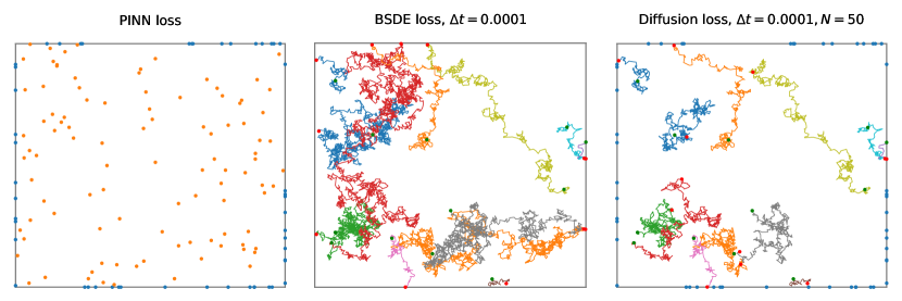
Figure 1: We illustrate the training data used for the three losses inside the unit square $\Omega=(0,1)^{2}$. The PINN loss in the left panel takes i.i.d. data points that are sampled from prescribed probability distributions in the domain $\Omega$ and on the boundary $\partial\Omega$ (in this case from uniform distributions). The BSDE loss (middle panel) uses trajectories associated to the SDE (3) that are started at random points $X_{0}$ (green points) and run until they hit the boundary (red points). The trajectories for the diffusion loss have a maximal length $\mathfrak{t}$ and therefore frequently start and end inside $\Omega$, as displayed in the right panel. The blue points for the PINN and diffusion losses indicate the additionally sampled boundary data.

The following proposition shows that the loss $\mathcal{L}_{\text{diffusion}}^{\mathfrak{t}}$ is indeed suitable for the boundary value problem (1).

Proposition 3.4.

Consider the diffusion loss as defined in (17), and assume that $b$ and $\sigma$ are globally Lipschitz continuous in $x$, uniformly in $t\in[0,T]$. Furthermore, assume the following Lipschitz and boundedness conditions on $f$, $g$ and $h$,

$$|f(x)| \leq C(1+|x|^{p}),$$

$$|g(x,t)| \leq C(1+|x|^{p}),$$

$$|h(t,x,y,z)| \leq C(1+|x|^{p}+|y|+|z|),$$

$$|h(t,x,y,z)-h(t,x,y^{\prime},z)| \leq C|y-y^{\prime}|,$$

$$|h(t,x,y,z)-h(t,x,y,z^{\prime})| \leq C|z-z^{\prime}|,$$

for appropriate constants $C,p\geq 0$ and all $x,y,z\in\Omega$, $t\in[0,T]$. Finally, assume that Assumption 1 is satisfied. Then for $\varphi\in\mathcal{F}$ the following are equivalent:

1. The diffusion loss vanishes on $\varphi$,

   $$\mathcal{L}_{\mathrm{diffusion}}^{\mathfrak{t}}(\varphi)=0.$$ (19)

2. $\varphi$ fulfills the boundary value problem (1).

Proof.

Denoting by $X_{s}$ the unique strong solution to (3), an application of Itô’s lemma to $\varphi(X_{s},s)$ yields

$$\varphi(X_{\mathcal{T}},\mathcal{T})=\varphi(X_{t_{0}},t_{0})+\int_{t_{0}}^{\mathcal{T}}(\partial_{s}+L)\varphi(X_{s},s)\,\mathrm{d}s+\int_{t_{0}}^{\mathcal{T}}\sigma^{\top}\nabla\varphi(X_{s},s)\cdot\mathrm{d}W_{s},$$ (20)

almost surely. Assuming that $\varphi$ fulfills the PDE (1a), it follows from the definition in (18a) that $\mathcal{L}_{\text{diffusion,int}}^{\mathfrak{t}}(\varphi)=0$. Similarly, the boundary conditions (1b) and (1c) imply that $\mathcal{L}_{\text{diffusion,T}}^{\mathfrak{t}}(\varphi)=\mathcal{L}_{\text{diffusion,b}}^{\mathfrak{t}}(\varphi)=0$. Consequently, we see that $\mathcal{L}_{\text{diffusion}}^{\mathfrak{t}}(\varphi)=0$.

For the converse direction, observe that $\mathcal{L}_{\text{diffusion}}^{\mathfrak{t}}(\varphi)=0$ implies that

$$\varphi(X_{\mathcal{T}},\mathcal{T})=\varphi(X_{t_{0}},t_{0})+\int_{t_{0}}^{\mathcal{T}}\sigma^{\top}\nabla\varphi(X_{s},s)\cdot\mathrm{d}W_{s}-\int_{t_{0}}^{\mathcal{T}}h(X_{s},s,\varphi(X_{s},s),\sigma^{\top}\nabla\varphi(X_{s},s))\,\mathrm{d}s,$$ (21)

almost surely, and that the same holds with $\varphi$ replaced by $V$. We proceed by defining the processes $\widetilde{Y}_{s}:=\varphi(X_{s},s)$ and $\widetilde{Z}_{s}:=\sigma^{\top}\nabla\varphi(X_{s},s)$, as well as $Y_{s}:=V(X_{s},s)$ and $Z_{s}:=\sigma^{\top}\nabla V(X_{s},s)$. By the assumptions on $\varphi$, $b$ and $\sigma$, the processes $Y$, $Z$, $\widetilde{Y}$ and $\widetilde{Z}$ are progressively measurable with respect to the filtration generated by $(W_{t})_{t\geq 0}$ and moreover square-integrable. Furthermore, the relation (21) shows that the pairs $(Y,Z)$ and $(\widetilde{Y},\widetilde{Z})$ satisfy a BSDE with terminal condition $\xi:=\varphi(X_{\mathcal{T}},\mathcal{T})$ on the random time interval $[t_{0},\mathcal{T}]$. Well-posedness of the BSDE (see [63, Theorems 1.2 and 3.2]) implies that $Y=\widetilde{Y}$ and $Z=\widetilde{Z}$, almost surely. Conditional on $t_{0}$ and $X_{t_{0}}$, we also have $V(X_{t_{0}},t_{0})=Y^{X_{t_{0}},t_{0}}=\widetilde{Y}^{X_{t_{0}},t_{0}}=\varphi(X_{t_{0}},t_{0})$, where the superscripts denote conditioning on the initial time $t_{0}$ and corresponding initial condition $X_{t_{0}}$, see [63, Theorems 2.4 and 4.3]. Hence, we conclude that $\varphi=V$, $\nu_{\Omega}\times[0,T]$-almost surely, and the result follows from the continuity of $\varphi$ and $V$ and the assumption that $\nu_{\Omega\times[0,T]}$ has full support. ∎

We have noted before that the diffusion loss combines aspects from the BSDE and PINN losses. In fact, it turns out that the diffusion loss can be interpreted as a specific type of interpolation between the two. The following proposition makes this observation precise.

Proposition 3.5 (Relation of the diffusion loss to the PINN and BSDE losses).

Let $\varphi\in\mathcal{F}$. Assuming that the measures $\nu_{\Omega\times[0,T]}$ in Definitions 2.1 and 3.1 coincide, we have that

$$\frac{\mathcal{L}_{\mathrm{diffusion,int}}^{\mathfrak{t}}(\varphi)}{\mathfrak{t}^{2}}\to\mathcal{L}_{\mathrm{PINN,int}}(\varphi),$$ (22)

as $\mathfrak{t}\to 0$. Moreover, if $\nu_{\Omega\times[0,T]}$ refers to the same measure in Definitions 2.1 and 2.4, then

$$\mathcal{L}_{\mathrm{diffusion,int}}^{\mathfrak{t}}(\varphi)\to\mathcal{L}_{\mathrm{BSDE}}(\varphi),$$ (23)

as $\mathfrak{t}\to\infty$.

Proof.

Itô’s formula shows that $\mathcal{L}_{\text{diffusion,int}}^{\mathfrak{t}}$ can be expressed as

$$\mathcal{L}_{\text{diffusion,int}}^{\mathfrak{t}}(\varphi) =\operatorname{\mathbb{E}}\left[\left(\int_{t_{0}}^{\mathcal{T}}(\partial_{s}+L)\varphi(X_{s},s)\,\mathrm{d}s+\int_{t_{0}}^{\mathcal{T}}h(X_{s},s,\varphi(X_{s},s),\sigma^{\top}\nabla\varphi(X_{s},s))\,\mathrm{d}s\right)^{2}\right],$$ (24)

which implies the limit (22) by dominated convergence, noting that $\mathcal{T}\to t_{0}$ as $\mathfrak{t}\to 0$, almost surely. The relation (23) follows immediately from the definition of $\mathcal{L}_{\mathrm{BSDE}}$ by noting that $\mathcal{T}\to\tau\wedge T$ as $\mathfrak{t}\to\infty$, almost surely. ∎

4 Extensions to elliptic PDEs and eigenvalue problems

In this section we show that the ideas reviewed and developed in the previous sections in the context of the parabolic boundary value problem (1) can straightforwardly be extended to the treatment of elliptic PDEs and certain eigenvalue problems (and in fact, the diffusion loss for parabolic problems could have been derived using [87, Section 2.2.3] as a starting point). To begin with, it is helpful to notice that the boundary value problem (1) can be written in the following slightly more abstract form:

Remark 4.1 (Compact notation).

Consider the operator $\mathcal{A}:=\partial_{t}+L$, the space-time domain $\Omega_{xt}:=\Omega\times[0,T)$ with (forward) boundary $\overrightarrow{\partial}\Omega_{xt}:=\Omega\times\{T\}\cup\partial\Omega\times[0,T]$, and the augmented variable $z=(x,t)^{\top}\in\Omega\times[0,T]$. Then problem (1) can be presented as

$$\mathcal{A}V(z)+h(z,V(z),\sigma^{\top}\nabla_{x}V(z)) =0,\qquad z\in\Omega_{xt},$$ (25a)

$$V(z) =k(z),\qquad z\in\overrightarrow{\partial}\Omega_{xt},$$ (25b)

with $k$ defined as in (10). Relying on (25), we can equivalently define the BSDE loss as

$$\mathcal{L}_{\text{BSDE}}(\varphi)=\mathbb{E}\Bigg{[} \Bigg{(}k(X_{\tau_{xt}},\tau_{xt})-\varphi(X_{t_{0}},t_{0})-\int_{t_{0}}^{\tau_{xt}}\sigma^{\top}\nabla\varphi(X_{s},s)\cdot\mathrm{d}W_{s}+\int_{t_{0}}^{\tau_{xt}}h(X_{s},s,\varphi(X_{s},s),\sigma^{\top}\nabla\varphi(X_{s},s))\,\mathrm{d}s\Bigg{)}^{2}\Bigg{]},$$ (26)

where $\tau_{xt}=\inf\{t>0:X_{t}\notin\Omega_{xt}\}$ is the first exit time from $\Omega_{xt}$. The PINN and diffusion losses can similarly be rewritten in terms of the space-time domain $\Omega_{xt}$ and exit time $\tau_{xt}$.

4.1 Elliptic boundary value problems

Removing the time dependence from the solution (and from the coefficients $b$ and $\sigma$ determining $L$) we obtain the elliptic boundary value problem

$$LV(x)+h(x,V(x),\sigma^{\top}\nabla V(x)) =0,\qquad x\in\Omega,$$ (27a)

$$V(x) =g(x),\qquad x\in\partial\Omega,$$ (27b)

with the nonlinearity $h\in C(\operatorname{\mathbb{R}}^{d}\times\operatorname{\mathbb{R}}\times\operatorname{\mathbb{R}}^{d},\operatorname{\mathbb{R}})$. In analogy to (9), the corresponding backward equation is given by

$$\mathrm{d}Y_{s}=-h(X_{s},Y_{s},Z_{s})\,\mathrm{d}s+Z_{s}\cdot\mathrm{d}W_{s},\qquad Y_{\tau}=g(X_{\tau}),$$ (28)

where $\tau=\{t>0:X_{t}\notin\Omega\}$ is the first exit time from $\Omega$. Given suitable boundedness and regularity assumptions on $h$ and assuming that $\tau$ is almost surely finite, one can show existence and uniqueness of solutions $Y$ and $Z$, which, as before, represent the solution $V$ and its gradient along trajectories of the forward process [63, Theorem 4.6].

Therefore, the BSDE, PINN and diffusion losses can be applied to (27) with minor modifications: Owing to the fact that there is no terminal condition, we set $f=0$ in (14), as well as $\alpha_{\text{T}}=0$ in (7) and (17), making (8b) and (18b) obsolete. With the same reasoning, we set $T=\infty$, incurring $\tau\wedge T=\tau$ and $\mathcal{T}=(t_{0}+\mathfrak{t})\wedge\tau$; these simplifications are relevant for the expressions (14) and (18a). Proposition 3.4 and its proof can straightforwardly be generalized to the elliptic setting. An algorithm for solving elliptic PDEs of the type (27) in the spirit of the BSDE loss has been suggested in [48], using the same approximation framework as in [19] (cf. Remark 2.7). We note that the solutions to linear elliptic PDEs often admit alternative variational characterizations in terms of energy functionals [22]. An approach using the Feynman-Kac formula has been considered in [24].

4.2 Elliptic eigenvalue problems

We can extend the algorithmic approaches from Sections 2 and 3 to eigenvalue problems of the form

$$LV(x) =\lambda V(x),\qquad x\in\Omega,$$ (29a)

$$V(x) =0,\qquad x\in\partial\Omega,$$ (29b)

corresponding to the choice $h(x,y,z)=-\lambda y$ in the elliptic PDE (27). Note, however, that $h$ now depends on the unknown eigenvalue $\lambda\in\operatorname{\mathbb{R}}$. Furthermore, we can consider nonlinear eigenvalue problems,

$$LV(x)+h(x,V(x),\sigma^{\top}\nabla V(x)) =\lambda V(x),\qquad x\in\Omega,$$ (30a)

$$V(x) =0,\qquad x\in\partial\Omega,$$ (30b)

with a general nonlinearity $h\in C(\operatorname{\mathbb{R}}^{d}\times\operatorname{\mathbb{R}}\times\operatorname{\mathbb{R}}^{d},\operatorname{\mathbb{R}})$.

For the linear problem (29) it is known that, given suitable boundedness and regularity assumption on $b$ and $\sigma$, there exists a unique principal eigenvalue with strictly positive eigenfunction in $\Omega$, see [8, Theorem 2.3]. This motivates us to consider the above losses, now depending on $\lambda$, as well as enhanced with an additional term, preventing the trivial solution $V\equiv 0$. We define

$$\mathcal{L}^{\mathrm{eigen}}(\varphi,\lambda)=\mathcal{L}_{\lambda}(\varphi)+\alpha_{\text{c}}\mathcal{L}_{\text{c}}(\varphi),$$ (31)

where $\mathcal{L}_{\lambda}(\varphi)$ stands for either the PINN, the BSDE, or the diffusion loss (with the nonlinearity $h$ depending on $\lambda$), $\mathcal{L}_{\text{c}}(\varphi)=(\varphi(x_{\text{c}})-1)^{2}$, and $\alpha_{\text{c}}>0$ is a weight. Here $x_{\text{c}}\in\Omega$ is chosen deterministically, preferably not too close to the boundary $\partial\Omega$. Clearly, the term $\mathcal{L}_{\text{c}}$ encourages $\varphi(x_{\text{c}})=1$, thus discouraging $\varphi\equiv 0$. We note that $V(x_{\text{c}})=1$ can be imposed on solutions to (29) without loss of generality, since the eigenfunctions are determined up to a multiplicative constant only. Avoiding $\phi\equiv 0$ for nonlinear eigenvalue problems of the form (30) needs to be addressed on a case-by-case basis; we present an example in Section 6.4.2.

The idea is now to minimize $\mathcal{L}^{\mathrm{eigen}}(\varphi,\lambda)$ with respect to $\varphi\in\mathcal{F}$ and $\lambda\in\operatorname{\mathbb{R}}$ simultaneously, while constraining the function $\varphi$ to be non-negative. According to the following proposition this is a valid strategy to determine the first eigenpair.

Proposition 4.2.

Let $\Omega$ be bounded, and assume that $L$ is uniformly elliptic, that is, there exist constants $c_{0},C_{0}>0$ such that

$$c_{0}|\xi|^{2}\leq\sum_{i,j=1}^{d}(\sigma\sigma^{\top})(x)\xi_{i}\xi_{j}\leq C_{0}|\xi|^{2},$$ (32)

for all $\xi\in\mathbb{R}^{d}$. Moreover, assume that $b$ is bounded. Let $\varphi\in\mathcal{F}$ with $\varphi\geq 0$ and assume that $\mathcal{L}_{\lambda}(\varphi)=0$ if and only if (29) is satisfied. Then the following are equivalent:

1. $\varphi$ is the principal eigenfunction for (29) with principal eigenvalue $\lambda$ and normalization $\varphi(x_{c})=1$.

2. $\mathcal{L}^{\mathrm{eigen}}(\varphi,\lambda)$ vanishes on the pair $(\varphi,\lambda)$,

   $$\mathcal{L}^{\mathrm{eigen}}(\varphi,\lambda)=0.$$ (33)

Remark 4.3.

The assumption that $\mathcal{L}_{\lambda}(\varphi)$ is equivalent to (29) is satisfied for any ‘reasonable’ loss function. For the diffusion loss, Proposition 3.4 establishes this condition whenever the coefficients in (29) are regular enough.

Proof.

It is clear that 1. implies 2. by the construction of (31). For the converse direction, notice that (33) implies $\varphi(x_{c})=1$ as well as (29), that is, $\varphi$ is an eigenfunction with eigenvalue $\lambda$. In conjunction with the constraint $\varphi\geq 0$, it follows by [8, Theorem 2.3] that $\varphi$ is the principal eigenfunction. ∎

An alternative approach towards (29) can be found in [30], where the eigenvalue problem is connected to a parabolic PDE and formulated as a fixed point problem.

5 From losses to algorithms

In this section we discuss some details regarding implementation aspects. For convenience, let us start by stating a prototypical algorithm based on the losses introduced in Sections 2 and 3:

Choose a parametrization $\mathbb{R}^{p}\ni\theta\mapsto\varphi_{\theta}$.

Initialize $\varphi_{\theta}$ (with a parameter vector $\theta\in\operatorname{\mathbb{R}}^{p}$).

Choose an optimization method descent, a batch size $K\in\mathbb{N}$ and a learning rate $\eta>0$. For PINN and diffusion losses choose weights $\alpha_{\text{int}},\alpha_{\text{b}},\alpha_{\text{T}}>0$ and batch sizes $K_{\text{b}},K_{\text{T}}\in\mathbb{N}$. For BSDE and diffusion losses choose a step-size $\Delta t>0$, for the diffusion loss choose a trajectory length $\mathfrak{t}>0$.

repeat

       Choose a loss function $\mathcal{L}$ from either (7), (14) or (17).

       Simulate data according to the chosen loss.

       Compute $\widehat{\mathcal{L}}(\varphi_{\theta})$ as a Monte Carlo version of $\mathcal{L}$.

       Compute $\nabla_{\theta}\widehat{\mathcal{L}}(\varphi_{\theta})$ using automatic differentiation.

       Update parameters: $\theta\leftarrow\theta-\eta\,\texttt{descent}(\nabla_{\theta}\widehat{\mathcal{L}}(\varphi_{\theta}))$.

until  convergence;

Result: $\varphi_{\theta}\approx V$.

Algorithm 1 Approximation of the solution $V$ to the boundary value problem (1).

Function approximation. In this paper, we rely on neural networks to provide the parametrization $\mathbb{R}^{p}\ni\theta\mapsto\varphi_{\theta}$ referred to in Algorithm 1 (but note that alternative function classes might offer specific benefits, see, for instance [75]). Standard feed-forward neural networks are given by

$$\varphi_{\theta}:\operatorname{\mathbb{R}}^{d}\to\operatorname{\mathbb{R}},\qquad\qquad\varphi_{\theta}(x)=A_{L}\varrho(A_{L-1}\varrho(\cdots\varrho(A_{1}x+b_{1})\cdots)+b_{L-1})+b_{L},$$ (34)

with a collection of matrices $A_{l}\in\operatorname{\mathbb{R}}^{n_{l}\times n_{l-1}}$ and vectors $b_{l}\in\operatorname{\mathbb{R}}^{n_{l}}$ comprising the learnable parameters, $\theta=(A_{l},b_{l})_{1\leq l\leq L}$. Here $L$ denotes the depth of the network, and we have $n_{0}=d$ as well as $n_{L}=1$. The nonlinear activation function $\varrho:\operatorname{\mathbb{R}}\to\operatorname{\mathbb{R}}$ is to be applied componentwise.

Additionally, we define the DenseNet [35, 22] as a variant of the feed-forward neural network (34), containing additional skip connections,

$$\varphi^{\mathrm{DenseNet}}_{\theta}(x)=A_{L}x_{L}+b_{L},$$ (35)

where $x_{L}$ is specified recursively as

$$y_{l+1}=\varrho(A_{l}x_{l}+b_{l}),\qquad x_{l+1}=(x_{l},y_{l+1})^{\top},\qquad x_{1}=x,$$ (36)

with $A_{l}\in\operatorname{\mathbb{R}}^{n_{l}\times\sum_{i=0}^{l-1}n_{i}}$ and $b_{l}\in\operatorname{\mathbb{R}}^{l}$ for $1\leq l\leq L-1$, $n_{0}=d$. Again, the collection of matrices $A_{l}$ and vectors $b_{l}$ comprises the learnable parameters.

Comparison of the losses (practical challenges). The PINN, BSDE and diffusion losses differ in the way training data is generated (see Figure 1 and Table 1(a)); hence, the corresponding implementations face different challenges (see Table 1(b)).

Table 1: Comparison of the different losses.

	PINN	BSDE	Diffusion
SDE simulation		✗	✗
boundary data	✗		✗

(a) The three losses can be characterized by how training data is generated.

	PINN	BSDE	Diffusion
Hessian computations	✗
exit time computations		✗
weight tuning	✗		✗
long runtimes		✗
discretization		✗	✗

(b) In this table we list potential challenges and drawbacks for the corresponding losses.

First, the BSDE and diffusion losses rely on trajectorial data obtained from the SDE (3), in contrast to the PINN loss (cf. the first row in Table 1(a)). As a consequence, the BSDE and diffusion losses do not require the computation of second-order derivatives, as those are approximated implicitly using Itô’s formula and the SDE (3), cf. the first row in Table 1(a). From a computational perspective, the PINN loss therefore faces a significant overhead in high dimensions when the diffusion coefficient $\sigma$ is not sparse (as the expression (8a) involves $d^{2}$ second-order partial derivatives). We notice in passing that an approach similar to the diffusion loss circumventing this problem has been proposed in [77, Section 3]. On the other hand, evaluating the BSDE and diffusion losses requires discretizing the SDE (3), incurring additional numerical errors (cf. the last row in Table 1(b) and the discussion below in Section 5.1).

Second, the PINN and diffusion losses incorporate boundary and final time constraints (see (1c) and (1b)) explicitly by sampling additional boundary data (see (8b), (8c), (18b), (18c) and cf. the second row in Table 1(a)). On the one hand, this approach necessitates choosing the weights $\alpha_{\text{int}},\alpha_{\text{b}},\alpha_{\text{T}}>0$; it is by now well established that while algorithmic performance depends quite sensitively on a judicious tuning of these weights, general and principled guidelines to address this issue are not straightforward (see, however, [80, 81, 82, 83]). Weight-tuning, on the other hand, is not required for implementations relying on the BSDE loss, as the boundary data is accounted for implicitly by the hitting event $\{(X_{t},t)\notin\Omega\times[0,T)\}$ and the corresponding first two terms on the right-hand side of (14). The hitting times $\tau=\inf\{t>0:X_{t}\notin\Omega\}$ may however be large, leading to a computational overhead in the generation of the training data (but see 5.2.1), and are generally hard to compute accurately (but see Section 5.1).

5.1 Simulation of diffusions and their exit times

The BSDE and diffusion losses rely on trajectorial data obtained from the stochastic process defined in (3). In practice, we approximate this SDE on a time grid $t_{0}\leq t_{1}\leq\dots\leq t_{N}$, for instance using the Euler-Maruyama scheme [47]

$$\widetilde{X}_{n+1}=\widetilde{X}_{n}+b(\widetilde{X}_{n},t_{n})\Delta t+\sigma(\widetilde{X}_{n},t_{n})\sqrt{\Delta t}\,\xi_{n+1},$$ (37)

or, to be precise, by its stopped version

$$\widehat{X}_{n+1}=\widehat{X}_{n}+\left(b(\widehat{X}_{n},t_{n})\Delta t+\sigma(\widehat{X}_{n},t_{n})\sqrt{\Delta t}\,\xi_{n+1}\right)\mathbbm{1}_{\mathcal{C}_{n+1}}$$ (38)

with step condition $\mathcal{C}_{n}:=\left\{\widetilde{X}_{n}\in\Omega\right\}\vee\left\{t_{n}\leq T\right\}$ and time-increment $t_{n+1}=t_{n}+\Delta t\,\mathbbm{1}_{\mathcal{C}_{n+1}}$, where $\Delta t$ is the step-size and $\xi_{n+1}\sim\mathcal{N}(0,\mathrm{Id}_{d\times d})$ are standard normally distributed random variables. We can then straightforwardly construct Monte Carlo estimator versions of either the BSDE or the diffusion loss. For example, the discrete version of the domain part of the diffusion loss (18a) reads

$$\widehat{\mathcal{L}}_{\mathrm{diffusion,int}}^{(K,N)}(\varphi) =\frac{1}{K}\sum_{k=1}^{K}\Bigg{(}\varphi(\widehat{X}_{N}^{(k)},t_{N}^{(k)})-\varphi(\widehat{X}_{0}^{(k)},t_{0}^{(k)})-\sum_{n=0}^{N-1}\sigma^{\top}\nabla\varphi(\widehat{X}_{n}^{(k)},t_{n}^{(k)})\cdot\xi_{n+1}^{(k)}\sqrt{\Delta t}\,\mathbbm{1}_{\mathcal{C}_{n}^{(k)}}$$ (39a)

$$\qquad\qquad\qquad+\sum_{n=0}^{N-1}h\left(\widehat{X}_{n}^{(k)},t_{n}^{(k)},\varphi(\widehat{X}_{n}^{(k)},t_{n}^{(k)}),\sigma^{\top}\nabla\varphi(\widehat{X}_{n}^{(k)},t_{n}^{(k)})\right)\Delta t\,\mathbbm{1}_{\mathcal{C}_{n}^{(k)}}\Bigg{)}^{2},$$ (39b)

where $K$ is the sample size, $N=\frac{\mathfrak{t}}{\Delta t}$ is the maximal discrete-time trajectory length, and $(\widehat{X}_{n}^{(k)})^{k=1...K}_{n=1...N}$ are independent copies of the iterates from (38). The Monte Carlo version of the BSDE loss can be formed analogously.

Given suitable growth and regularity assumptions on the coefficients, the discretization errors of the forward and backward processes are of order $\sqrt{\Delta t}$ [47, 85], cf. also [29] for a numerical analysis on the original version of the BSDE loss. However, the stopped Euler-Maruyama scheme (38) incurs additional errors due to the approximation of the first exit times from $\Omega$. In the two left panels of Figure 2 we illustrate this problem by displaying multiple “last locations” obtained according to (38), using two different step-sizes $\Delta t$. Clearly, all these points should in principle lie on the boundary, (naively) requiring a computationally costly small step-size.

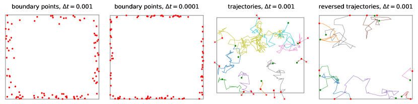
Figure 2: Illustration of the boundary data in the BSDE method.

Sophisticated approaches towards the accurate simulation of exit times for diffusions discretizing exit times have been put forward, see, e.g. [15, 58, 33]. For our purposes, however, it is not essential to compute the exit times, as long as the simulated trajectories are stopped accurately. We therefore suggest the following two attempts that aim at improving the sampling of boundary data:

1. Rescaling: Start $X_{0}$ randomly in $\Omega$, simulate the trajectory and stop once the boundary has been crossed, however scale the last time step in such a way that the trajectory exactly ends on $\partial\Omega$.

2. Time-reversal: Start $X_{0}$ on the boundary $\partial\Omega$ and simulate the trajectory for a given time $T$ (unless it hits the boundary again before time $T$, in this case stop the trajectory accordingly or resimulate). Then reverse the process such that the reversed process exactly ends on the boundary.

An illustration of these two strategies can be found in the two right panels of Figure 2. In our numerical experiments we have found that both rescaling and time-reversal improves the performance of the BSDE method somewhat, but further research is needed.

5.2 Further modifications of the losses

In the following we discuss modifications of the PINN, BSDE and diffusion losses, relating also to versions that have appeared in the literature before.

5.2.1 Forward control

We can modify the SDE-based BSDE and diffusion losses by including control terms $v\in C(\operatorname{\mathbb{R}}^{d}\times[0,T],\operatorname{\mathbb{R}}^{d})$ in the forward process (3), yielding the controlled diffusion

$$\mathrm{d}X^{v}_{s}=\left(b(X^{v}_{s},s)+\sigma(X^{v}_{s},s)v(X^{v}_{s},s)\right)\mathrm{d}s+\sigma(X^{v}_{s},s)\,\mathrm{d}W_{s}.$$ (40)

Applying Itô’s formula we may obtain losses similar to those considered in Section 2 and 3. For instance, alternative versions of the diffusion loss take the form

$$\begin{split}\mathcal{L}_{\text{diffusion,int}}^{\mathfrak{t},v}(\varphi)&=\operatorname{\mathbb{E}}\Bigg{[}\Bigg{(}\varphi(X^{v}_{\mathcal{T}},\mathcal{T})-\varphi(X^{v}_{t_{0}},t_{0})-\int_{t_{0}}^{\mathcal{T}}\sigma^{\top}\nabla\varphi(X_{s},s)\cdot\mathrm{d}W_{s}\\ &\qquad\qquad+\int_{t_{0}}^{\mathcal{T}}\left[h(X_{s}^{v},s,\varphi(X_{s}^{v},s),\sigma^{\top}\nabla\varphi(X_{s}^{v},s))-v(X^{v}_{s},s)\cdot\sigma^{\top}\nabla\varphi(X_{s}^{v},s)\right]\mathrm{d}s\Bigg{)}^{2}\Bigg{]},\end{split}$$ (41)

replacing (18a). We note in passing that Proposition 3.4 extends straightforwardly to $\mathcal{L}_{\text{diffusion,int}}^{\mathfrak{t},v}$ under the assumption that $v$ satisfies appropriate Lipschitz and growth conditions.

Similar considerations apply for the BSDE loss, noting that for solutions to the generalized BSDE system [62]

$$\mathrm{d}X^{v}_{s} =\left(b(X^{v}_{s},s)+\sigma(X^{v}_{s},s)v(X^{v}_{s},s)\right)\mathrm{d}s+\sigma(X^{v}_{s},s)\,\mathrm{d}W_{s},\qquad\qquad\qquad\qquad X^{v}_{t_{0}}=x_{\mathrm{init}},$$ (42a)

$$\mathrm{d}Y_{s}^{v} =-h(X^{v}_{s},s,Y^{v}_{s},Z^{v}_{s})\,\mathrm{d}s+v(X^{v}_{s},s)\cdot Z_{s}^{v}\,\mathrm{d}s+Z_{s}^{v}\cdot\mathrm{d}W_{s},\qquad\qquad Y_{T}^{v}=k(X^{v}_{T\wedge\tau},T\wedge\tau),$$ (42b)

we still have the relations

$$Y_{s}^{v}=V(X_{s}^{v},s),\qquad Z_{s}^{v}=\sigma^{\top}\nabla V(X_{s}^{v},s)$$ (43)

for suitable $v\in C(\operatorname{\mathbb{R}}^{d}\times[0,T],\operatorname{\mathbb{R}}^{d})$, analogously to (11). This immediately incurs the family of losses

$$\begin{split}\mathcal{L}_{\text{BSDE}}^{v}(\varphi)=\mathbb{E}\Bigg{[}&\Bigg{(}f(X^{v}_{\tau\wedge T})\mathbbm{1}_{\tau\wedge T=T}+g(X^{v}_{\tau\wedge T},\tau\wedge T)\mathbbm{1}_{\tau\wedge T=\tau}-\varphi(X^{v}_{t_{0}},t_{0})-\int_{t_{0}}^{\tau\wedge T}\sigma^{\top}\nabla\varphi(X^{v}_{s},s)\cdot\mathrm{d}W_{s}\\ &\quad+\int_{t_{0}}^{\tau\wedge T}\left(h(X^{v}_{s},s,\varphi(X_{s},s),\sigma^{\top}\nabla\varphi(X_{s},s))-v(X^{v}_{s},s)\cdot\sigma^{\top}\nabla\varphi(X_{s}^{v},s)\right)\mathrm{d}s\Bigg{)}^{2}\Bigg{]},\end{split}$$ (44)

parametrized by $v\in C(\operatorname{\mathbb{R}}^{d}\times[0,T],\operatorname{\mathbb{R}}^{d})$.

Adding a control to the forward process can be understood as driving the data generating process into regions of interest, for instance possibly alleviating the problem that exit times might be large (see Table 1(b) and the corresponding discussion). Identifying suitable forward controls might be an interesting topic for future research (we refer to [62] for some systematic approaches in this respect relating to Hamilton-Jacobi-Bellman PDEs).

5.2.2 Approximating the gradient of the solution

The constraints imposed by the BSDE system (9) can be enforced by losses that are slightly different from Definition 2.4. Going back to [19], we can for instance use the fact that the backward process $Y$ can be written in a forward way, yielding the discrete-time process

$$\widehat{Y}_{n+1}=\widehat{Y}_{n}-h(\widehat{X}_{n},t_{n},\widehat{Y}_{n},\widehat{Z}_{n})\Delta t+\widehat{Z}_{n}\cdot\xi_{n+1}\sqrt{\Delta t}.$$ (45)

The scheme (45) is explicit, the unknowns being $\widehat{Y}_{0}$ and $\widehat{Z}_{n}$, for $n\in\{0,\dots,N-1\}$. This motivates approximating the single parameter $y_{0}\approx\widehat{Y}_{0}\in\operatorname{\mathbb{R}}$ as well as the vector fields $\phi\approx\sigma^{\top}\nabla V\in C(\operatorname{\mathbb{R}}^{d}\times[0,T],\operatorname{\mathbb{R}}^{d})$, rather than $V$ directly. This approach gives rise to the loss

$$\begin{split}\mathcal{L}_{\mathrm{BSDE-2}}(\phi,y_{0})=\mathbb{E}\Bigg{[}&\Bigg{(}f(X_{\tau\wedge T})\mathbbm{1}_{\tau\wedge T=T}+g(X_{\tau\wedge T},\tau\wedge T)\mathbbm{1}_{\tau\wedge T=\tau}-y_{0}-\int_{0}^{\tau\wedge T}\phi(X_{s},s)\cdot\mathrm{d}W_{s}\\ &\qquad+\int_{0}^{\tau\wedge T}h(X_{s},s,Y_{s},\phi(X_{s},s))\,\mathrm{d}s\Bigg{)}^{2}\Bigg{]}.\end{split}$$ (46)

In this setting $X_{0}$ has to be chosen deterministically; we note that a potential drawback is thus that the solution is only expected to be approximated accurately in regions that can be reached by the forward process $X_{t}$ (starting at $X_{0}$) with sufficiently high probability. It has been shown in [62] that alternative losses (like the log-variance loss) can be considered whenever the nonlinearity $h$ only depends on the solution through its gradient, in which case the extra parameter $y_{0}$ can be omitted.

5.2.3 Penalizing deviations from the discrete scheme

Another approach that is rooted in the discrete-time backward process (45) has been suggested in [70] for problems on unbounded domains. It relies on the idea to penalize deviations from (45), for each $n\in\{0,\dots,N-1\}$ (cf. also [36, 75], where however an implicit scheme and backward iterations are used). Aiming for $\widehat{Y}_{n}\approx\varphi(\widehat{X}_{n},t_{n})$, $\widehat{Z}_{n}\approx\sigma^{\top}\nabla\varphi(\widehat{X}_{n},t_{n})$, this motivates the loss

$$\widehat{\mathcal{L}}^{(K,N)}_{\mathrm{BSDE-3}}(\varphi)=\alpha_{\text{int}}\widehat{\mathcal{L}}^{(K,N)}_{\mathrm{BSDE-3,int}}(\varphi)+\alpha_{\text{b}}\widehat{\mathcal{L}}^{(K,N)}_{\mathrm{BSDE-3,b}}(\varphi)$$ (47)

with interior part

$$\widehat{\mathcal{L}}^{(K,N)}_{\mathrm{BSDE-3,int}}(\varphi)=\frac{1}{K}\sum_{k=1}^{K}\sum_{n=0}^{N-1}\left(\varphi(\widehat{X}_{n+1}^{(k)})-\varphi(\widehat{X}_{n}^{(k)})+h\left(\widehat{X}_{n}^{(k)},\varphi(\widehat{X}_{n}^{(k)}),\sigma^{\top}\nabla\varphi(\widehat{X}_{n}^{(k)})\right)\Delta t-\sigma^{\top}\nabla\varphi(\widehat{X}_{n}^{(k)})\xi_{n+1}\sqrt{\Delta t}\right)^{2}$$ (48)

and boundary term

$$\widehat{\mathcal{L}}^{(K,N)}_{\mathrm{BSDE-3,b}}(\varphi)=\frac{1}{K}\sum_{k=1}^{K}\left(\varphi(\widehat{X}_{N}^{(k)})-g(\widehat{X}_{N}^{(k)})\right)^{2}.$$ (49)

A generalization to equations posed on bounded domains is straightforward. We also note that in contrast to the diffusion loss, (47) does not seem to naturally derive from a continuous-time formulation. Interestingly, $\widehat{\mathcal{L}}^{(K,N)}_{\mathrm{BSDE-3}}$ can be related to the diffusion loss via Jensen’s inequality,

$$\widehat{\mathcal{L}}_{\mathrm{diffusion,int}}^{(K,N)}(\varphi)\leq N\widehat{\mathcal{L}}^{(K,N)}_{\mathrm{BSDE-3,int}}(\varphi).$$ (50)

Yet another approach that is based on a discrete backward scheme is the following. Let us initialize $\widehat{Y}_{0}=\varphi(\widehat{X}_{0},0)$ and simulate

$$\widehat{Y}_{n+1}=\widehat{Y}_{n}-h(\widehat{X}_{n},\widehat{Y}_{n},\sigma^{\top}\nabla\varphi(\widehat{X}_{n},t_{n}))\Delta t+\sigma^{\top}\nabla\varphi(\widehat{X}_{n},t_{n})\cdot\xi_{n+1}\sqrt{\Delta t},$$ (51)

for $n\in\{0,\dots,N-1\}$, where, similarly to (46), but in in contrast to (48), only $\widehat{Z}_{n}$ is replaced by its approximation $\sigma^{\top}\nabla\varphi(\widehat{X}_{n},t_{n})$ while $\widehat{Y}_{n}$ is retained from previous iteration steps. Again penalizing deviations from the discrete-time scheme, we can now introduce the loss

$$\widehat{\mathcal{L}}^{(K,N)}_{\mathrm{BSDE-4}}(\varphi)=\frac{\alpha_{1}}{K}\sum_{k=1}^{K}\sum_{n=0}^{N}\left(\varphi(\widehat{X}_{n}^{(k)},t_{n})-\widehat{Y}_{n}^{(k)}\right)^{2}+\frac{\alpha_{2}}{K}\sum_{k=1}^{K}\left(\varphi(X_{b}^{(k)})-g(X_{b}^{(k)})\right)^{2}.$$ (52)

Both in $\mathcal{L}_{\mathrm{BSDE-3}}$ and $\mathcal{L}_{\mathrm{BSDE-4}}$ the deterministic initial condition $\widehat{X}_{0}$ at $t=0$ can be replaced by random choices $(\widehat{X}_{t_{0}},t_{0})\sim\nu_{\Omega\times[0,T]}$, adjusting the sums in (48) and (52) accordingly.

6 Numerical experiments

In this section we provide several numerical examples of high-dimensional parabolic and elliptic PDEs that shall demonstrate the performances of Algorithm 1 using the different loss functions introduced previously. We focus on the PINN, BSDE and diffusion losses from Sections 2 and 3 since their modified versions from Section 5.2 in general led to similar or worse performances. If not specified otherwise, the approximation of $\varphi$ relies on a DenseNet architecture defined in (35) with ReLU activation function and four hidden layers with $d+20$, $d$, $d$, $d$ units respectively (recall that $d$ specifies the dimension). The optimization is carried out using the Adam optimizer [46] with standard parameters and learning rate $\eta=0.001$. Throughout, we take $K_{\text{int}}=200$ samples inside the domain $\Omega$ and (for the PINN and diffusion losses) $K_{\text{b}}=50$ samples on the boundary, per gradient step. For the SDE discretization we choose a step-size of $\Delta t=0.001$. The weight configurations for the PINN and diffusion losses are optimized manually; we then only report the results for the optimal settings (see the discussion on weight-tuning in Section 5). We refer to the code at https://github.com/lorenzrichter/path-space-PDE-solver.

6.1 Nonlinear toy problems

Let us start with a nonlinear toy problem for which analytical reference solutions are available. Throughout this subsection, the domain of interest is taken to be the unit ball $\Omega=\{x\in\operatorname{\mathbb{R}}^{d}:|x|<1\}$.

6.1.1 Elliptic problem with Dirichlet boundary data

We first consider an elliptic boundary value problem of the form (27). Let $\gamma\in\operatorname{\mathbb{R}}$ and choose

$$b(x,t)=\mathbf{0},\qquad\sigma(x,t)=\sqrt{2}\,\mathrm{Id}_{d\times d},\qquad g(x)=e^{\gamma},\\$$ (53a)

$$h(x,y,z)=-2\gamma y(\gamma|x|^{2}+d)+\sin\left(e^{2\gamma|x|^{2}}-y^{2}\right).$$ (53b)

It is straightforward to verify that

$$V(x)=e^{\gamma|x|^{2}}$$ (54)

is the unique solution to (27).

We consider $d=50$ and set $\gamma=1$. For the PINN and diffusion losses the optimized weights are given by $\alpha_{\text{int}}=10^{-5}$, $\alpha_{\text{b}}=1$ and $\alpha_{\text{int}}=0.1$, $\alpha_{\text{b}}=1$, respectively. We sample the data uniformly and take a maximal (discrete-time) trajectory length of $N=20$ (i.e. $\mathfrak{t}=0.02$) for the diffusion loss. In Figure 3 (left panel) we display the average relative errors $\frac{|\varphi(x)-V(x)|}{V(x)}$ as a function of $r=|x|$. Due to volume distortion in high dimensions, very few samples are drawn close to the center of the ball, and hence the numerical results appear to be unreliable for $r\leq 0.8$. While this effect could be alleviated by changing the measure $\nu_{\Omega}$ accordingly, we content ourselves here with a comparison for $r\in[0.8,1]$. In the right panel we display the $L^{2}$ error during the training iterations evaluated on uniformly sampled test data. We observe that the PINN and diffusion losses yield similar results and that the BSDE loss performs worse, in particular close to the boundary. We attribute this effect to the challenges inherent in the simulation of hitting times, see Section 5.1.

Figure 3: Left: Average relative errors as a function of $r=|x|$ evaluated on uniformly sampled data for the three losses smoothed with a moving average over $500$ data points. For the training the diffusion loss relies on trajectory lengths of $\mathfrak{t}=0.02$. Right: $L^{2}$ error during the training iterations evaluated on uniformly sampled test data.

In the diffusion loss as stated in Definition 3.1 we are free to choose the length $\mathfrak{t}$ of the forward trajectories, which affects the generated training data. Let us therefore investigate how different choices of $\mathfrak{t}$ influence the performance of Algorithm 1. To this end, we consider again the elliptic problem from Section 6.1.1 and vary $\mathfrak{t}$. To be precise, let us fix different step-sizes $\Delta t$ and vary the Euler steps $N$ (recalling that $\mathfrak{t}=N\Delta t$), once choosing the weight $\alpha_{\text{int}}=0.1$, as before, and once by considering $\alpha_{\text{int}}=10$. For the former choice we can see in Figure 4(a) that larger trajectories tend to be better until a plateau is reached, whereas for the latter it turns out that there seems to be an optimal choice of the trajectory length, as displayed in Figure 4(b).

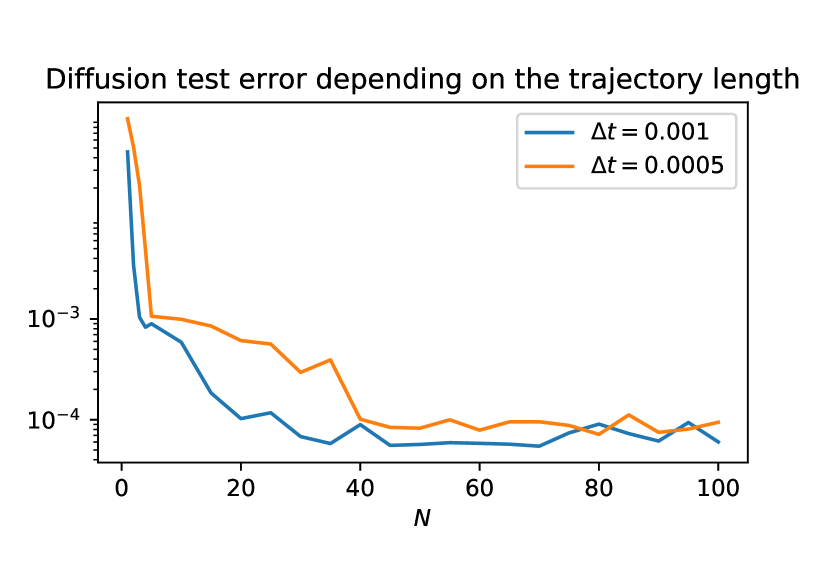
(a) Weight $\alpha_{\text{int}}=0.1$.

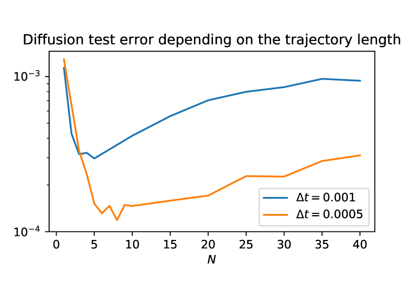
(b) Weight $\alpha_{\text{int}}=10$.

Figure 4: We display the $L^{2}$ error that one attains when using different choices of the maximal Euler steps $N$ in the diffusion loss for different discretization step-sizes $\Delta t$.

6.1.2 Elliptic problem requiring the full Hessian matrix

We consider the setting specified in (53), replacing however the diffusion coefficient and the nonlinearity by

$$\sigma(x,t)=\sqrt{\frac{2}{d}}\begin{pmatrix}1&\cdots&1\\ \vdots&\ddots&\vdots\\ 1&\cdots&1\end{pmatrix},\qquad h(x,y,z)=-2\gamma y\left(\gamma\sum_{i,j=1}^{d}x_{i}x_{j}+d\right)+\sin\left(e^{2\gamma|x|^{2}}-y^{2}\right),$$ (55)

respectively. Again, we can check that $V(x)=e^{\gamma|x|^{2}}$ is the unique solution to the corresponding boundary value problem. Since $\sigma$ is not diagonal anymore, the differential operator (2) contains the full Hessian matrix of second-order derivatives of the candidate solution $\varphi$. As discussed in Section 5 (see Table 1(b)) this particularly impacts the runtime of the PINN method since all derivatives need to be computed explicitly. For the BSDE and diffusion losses, on the other hand, second-order derivatives are implicitly approximated using the underlying Brownian motion and we therefore do not expect significantly longer runtimes.

Let us consider $d=20$ and $\gamma=1$ and as before choose $N=20$ (i.e. $\mathfrak{t}=0.02$) for the diffusion loss. In Figure 5 we display the $L^{2}$ error during the training process, plotted against the number of gradient steps (left panel) and against the runtime (right panel). As expected, the PINN loss takes significantly longer. This effect should become even more pronounced with growing state space dimension $d$.

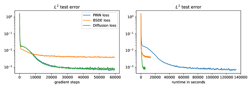
Figure 5: $L^{2}$ error during the training process evaluated on test data for the three losses, plotted against the number of gradient steps (left panel) and against the runtime (right panel). The diffusion loss relies on trajectory lengths of $\mathfrak{t}=0.02$.

6.1.3 Parabolic problem with Neumann boundary data

Let us now consider the parabolic problem (1), with the Dirichlet boundary condition (1c) replaced by its Neumann counterpart

$$\partial_{\vec{n}}V(x,t)=g^{N}(x,t),\qquad(x,t)\in\partial\Omega\times[0,T].$$ (56)

Here, $\partial_{\vec{n}}V:=\nabla V\cdot\vec{n}$ refers to the (outward facing) normal derivative at the boundary $\partial\Omega$. We take

$$b(x,t)=\mathbf{0},\qquad\sigma(x,t)=\sqrt{2}\,\mathrm{Id}_{d\times d},\qquad f(x)=e^{\gamma|x|^{2}+T},\qquad g^{N}(x,t)=2\gamma e^{\gamma+t},\\$$ (57a)

$$h(x,t,y,z)=-y(2\gamma(2\gamma|x|^{2}+d)+1)+\sin\left(e^{2\gamma|x|^{2}+2t}-y^{2}\right).$$ (57b)

In this case,

$$V(x,t)=e^{\gamma|x|^{2}+t}$$ (58)

provides the unique solution.

We choose $d=20$ and $\gamma=1$. For the diffusion loss we take $N=25$ (i.e. $\mathfrak{t}=0.025$) for the trajectory length. In the left and central panels of Figure 6 we display the approximated solutions along the curve $\left\{(\kappa,\dots,\kappa)^{\top}:\kappa\in[-1/\sqrt{d},1/\sqrt{d}]\right\}$ for two different times. We can see that both the diffusion and the PINN loss work well, with small advantages for the PINN loss. The right panel displays the $L^{2}$ test error over the iterations and confirms this observation.

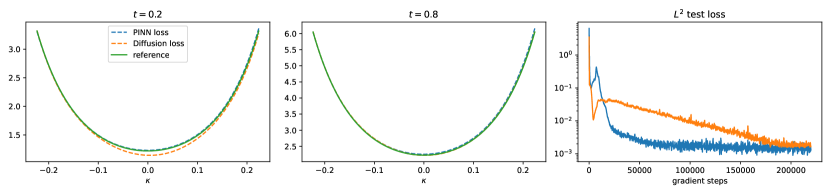
Figure 6: Left and central panel: Approximations along a curve for two different times using the diffusion and PINN losses. Right: $L^{2}$ test error along the training iterations.

6.2 Committor functions

Committor functions are important quantities in molecular dynamics as they specify likely transition pathways as well as transition rates between (potentially metastable) regions or conformations of interest [56, 21]. Since for most practical applications those functions are high-dimensional and hard to compute, there have been recent attempts to approach this problem using neural networks [45, 53, 76]. Based on the fact that committor functions fulfill elliptic boundary value problems, we can rely on the methods discussed in this paper.

For an $\mathbb{R}^{d}$-valued stochastic process $(X_{t})_{t\geq 0}$ with continuous sample paths and two disjoint open sets $A,B\subset\mathbb{R}^{d}$, the committor function $V$ computes the probability of $X$ hitting $A$ before $B$ when starting in $x\in\mathbb{R}^{d}$, that is,

$$V(x)=\mathbb{P}(\tau_{B}<\tau_{A}|X_{0}=x)=\operatorname{\mathbb{E}}[\mathbbm{1}_{B}(X_{\tau})|X_{0}=x].$$ (59)

Here, $\tau_{A}=\inf\{t>0:X_{t}\in A\}$ and $\tau_{B}=\inf\{t>0:X_{t}\in B\}$ refer to the hitting times corresponding to the sets $A$ and $B$. In the case when $(X_{t})_{t\geq 0}$ is given as the unique strong solution to the SDE (3), it can be shown via the Kolmogorov backward PDE [66, Section 2.5] that $V$ fulfills the elliptic boundary value problem

$$LV=0,\qquad V|_{\partial A}=0,\qquad V|_{\partial B}=1,$$ (60)

where $L$ as in (2) refers to the associated infinitesimal generator, see, for instance, [21]. In the notation of (27) we have $\Omega=\operatorname{\mathbb{R}}^{d}\setminus(A\cup B)$, $h=0$ and $g(x)=\mathbbm{1}_{B}(x)$.

Following [32, Section V.A], we consider $(X_{t})_{t\geq 0}$ to be a standard Brownian motion starting at $x\in\mathbb{R}^{d}$, that is, $X_{t}=x+W_{t}$, corresponding to $b=\mathbf{0}$ and $\sigma=\mathrm{Id}_{d\times d}$ in (3). The sets $A$ and $B$ are defined as

$$A=\{x\in{\operatorname{\mathbb{R}}}^{d}:|x|<a\},\qquad B=\{x\in{\operatorname{\mathbb{R}}}^{d}:|x|>b\},$$ (61)

with $b>a>0$. Hence, in this case the committor function describes the statistics of leaving a spherical shell through one of its boundaries. The solution takes the form

$$V(x)=\frac{a^{2}-|x|^{2-d}a^{2}}{a^{2}-b^{2-d}a^{2}},$$ (62)

for $d\geq 3$. Let us consider $d=10$ as well as $a=1$, $b=2$. We take a DenseNet with the $\tanh$ activation function and compare the three losses against each other. For the diffusion loss we take $N=50$ (i.e. $\mathfrak{t}=0.05$) for the trajectory length. In Figure 7 we display the approximated solutions along a curve $\left\{(\kappa,\dots,\kappa)^{\top}:\kappa\in[a/\sqrt{d},b/\sqrt{d}]\right\}$ in the left panel, realizing that in particular the PINN and diffusion losses lead to good approximations. This can also be observed in the right panel, where we plot a moving average of the $L^{2}$ error on test data based on a moving window of length $200$. The BSDE loss appears to be especially error-prone close to the left end-point of the curve displayed in Figure 7, that is, close to the inner shell. Due to the volume distortion in high dimensions, few samples are drawn according to $\nu_{\Omega}$ for small values of $|x|$, see Figure 8. We hence conclude that in this example, the BSDE loss suffers particularly from the relative sparsity of the samples, possibly in conjunction with numerical errors made while estimating the hitting times at the inner shell (see Section 5.1).

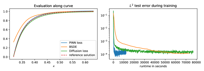
Figure 7: Left: approximations of the $10$-dimensional committor function evaluated along a curve. Right: moving average of the test $L^{2}$ error along the training iterations.

Figure 8: We plot the approximated committor functions evaluated at $10000$ points uniformly sampled from the domain $\Omega$ (blue dots) and compare those to the reference solution (orange line) as a function of $r=|x|$.

6.3 Parabolic Allen-Cahn equation on an unbounded domain

The Allen-Cahn equation in $d=100$ has been suggested as a benchmark problem in [19]. It is an example of a parabolic PDE posed on an unbounded domain,

$$(\partial_{t}+L)V(x,t)+V(x,t)-V^{3}(x,t) =0,\qquad (x,t)\in\operatorname{\mathbb{R}}^{d}\times[0,T],$$ (63a)

$$V(x,T) =f(x),\qquad x\in\operatorname{\mathbb{R}}^{d},$$ (63b)

with $f(x)=\left(2+\frac{2}{5}|x|^{2}\right)^{-1}$ and $T=\frac{3}{10}$. We restrict attention to the ball $\{x\in\operatorname{\mathbb{R}}^{d}:|x|<r\}$ with radius $r=7$, from which we sample the initial points of the trajectories for the BSDE and diffusion losses, or the training data for the PINN loss, respectively. Instead of using the uniform distribution on this set, we consider sampling uniformly on a box around the origin with side length $2$ and multiplying each data point $x$ by $\frac{r}{|x|}$. In contrast to uniform sampling, this approach generates more samples close to the origin, which we observe to slightly improve the accuracy of the obtained solutions. For the diffusion loss we choose $N=25$ (i.e. $\mathfrak{t}=0.025$) for the trajectory length. We compare our approximations to a reference solution at $x_{0}=(0,\dots,0)^{\top}$ for different times $t\in[0,T]$ that is provided by a branching diffusion method specified in [19]. In Figure 9 we see that all three attempts match this reference solution, with very minor advantages (for instance at the right end point) for the PINN and diffusion losses. In Table 2 we display the computation times until convergence, realizing that the BSDE loss needs significantly longer, which is in accordance with Remark 3.2 and might be explained by the fact that $\mathfrak{t}<T$. We note that the computation times are longer in comparison to e.g. [19] since we aim for a solution on a given domain, whereas other attempts only strive for approximating the solution at a single point.

Figure 9: Approximation of the solution to an Allen-Cahn equation in $d=100$ using different losses compared to a reference solution at $x_{0}=(0,\dots,0)^{\top}$ for different times $t\in[0,T]$.

Computation time
PINN loss	$325.46$ min
BSDE loss	$4280.68$ min
Diffusion loss	$194.38$ min

Table 2: Computation times until convergence.

6.4 Elliptic eigenvalue problems

In this section we provide two examples for the approximation of principal eigenvalues and corresponding eigenfunctions. The first one is a linear problem and therefore Proposition 4.2 assures that the minimization of an appropriate loss as in (31) leads to the desired solution. The second example is a nonlinear eigenvalue problem, for which we can numerically show that our algorithm still provides the correct solution.

6.4.1 Fokker-Planck equation

As suggested in [30], we aim at computing the principal eigenpair associated to a Fokker-Planck operator, defined by

$$LV=-\Delta V-\nabla\cdot(V\nabla\Psi),$$ (64)

for $V:\Omega\to\operatorname{\mathbb{R}}$ on the domain $\Omega=[0,2\pi]^{d}$, and where $\Psi(x)=\sin\left(\sum_{i=1}^{d}c_{i}\cos(x_{i})\right)$ is a potential with constants $c_{i}\in[0.1,1]$, assuming periodic boundary conditions. This results in the eigenvalue problem

$$\Delta V(x)+\nabla\Psi(x)\cdot\nabla V(x)+\Delta\Psi(x)V(x)=-\lambda V(x),$$ (65)

and

$$V(x)=e^{-\Psi(x)}$$ (66)

is an eigenfunction associated to the principal eigenvalue $\lambda=0$, see [66, Section 4.7]. We choose $c_{i}=0.1$, $i=1,\ldots,d$, and approach this problem in dimension $d=5$ following Section 4.2, i.e. by minimizing the loss (31), where for $\mathcal{L}$ we choose the diffusion loss with $N=20$ (i.e. $\mathfrak{t}=0.02$) and the periodic boundary condition is encoded via the term (15). Here and in the following eigenvalue problem the positivity of the approximating function is enforced by adding a ReLU function after the last layer of the DenseNet.

In the left panel of Figure 10 we display the approximated eigenfunction along the curve $\left\{(\kappa,\dots,\kappa)^{\top}:\kappa\in[0,2\pi]\right\}$ and compare it to the reference solution. In the central panel we show the $L^{2}$ error w.r.t. the reference solution evaluated on uniformly sampled test data along the training iterations. The right panel displays the moving average of the absolute value of the eigenvalue taken over a moving window of $100$ gradient steps (since the true value is $\lambda=0$ it is not possible to compute a relative error here). We see that both the eigenfunction and the eigenvalue are approximated sufficiently well.

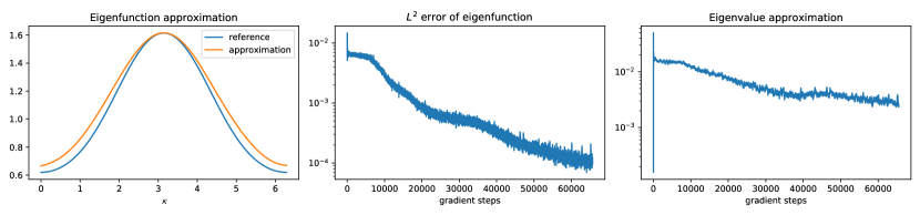
Figure 10: Left: Approximation and reference of the eigenfunction corresponding to the principal eigenvalue of the Fokker-Planck operator (64). Middle: $L^{2}$ error w.r.t. test data along the training iterations. Right: Moving average of the absolute value of the approximated eigenvalue along the gradient steps.

6.4.2 Nonlinear Schrödinger equation

Let us now consider a nonlinear eigenvalue problem. Again following [30], we consider the nonlinear Schrödinger operator including a cubic term that arises from the Gross-Pitaevskii equation for the single-particle wave function in a Bose-Einstein condensate [27, 69]. To be precise, we consider

$$\Delta V(x)-V^{3}(x)-\Psi(x)V(x)=-\lambda V(x),$$ (67)

where

$$\Psi(x)=-\frac{1}{c^{2}}\exp\left(\frac{2}{d}\sum_{i=1}^{d}\cos x_{i}\right)+\sum_{i=1}^{d}\left(\frac{\sin^{2}(x_{i})}{d^{2}}-\frac{\cos x_{i}}{d}\right)-3.$$ (68)

One can show that

$$V(x)=\frac{1}{c}\exp\left(\frac{1}{d}\sum_{i=1}^{d}\cos x_{i}\right)$$ (69)

is the eigenfunction corresponding to the principal eigenvalue $\lambda=-3$, where $c$ is determined from the normalization $\int_{\Omega}V^{2}(x)\,\mathrm{d}x=|\Omega|$. We add the latter constraint into the loss function by replacing the term $\mathcal{L}_{c}(\varphi)$ in (31) with $\mathcal{L}_{n}(\varphi)=\left(\operatorname{\mathbb{E}}\left[\varphi(X)^{2}\right]-1\right)^{2}$, where the distribution of $X$ is uniform on $\Omega=[0,2\pi]^{d}$. We again rely on the diffusion loss with a trajectory length of $N=20$ (i.e. $\mathfrak{t}=0.02$). Figure 11 shows the approximate solution of the eigenfunction in $d=5$ evaluated along the curve $\left\{(\kappa,\dots,\kappa)^{\top}:\kappa\in[0,2\pi]\right\}$ as well as its $L^{2}$ error and the relative error of the approximated eigenvalue along the training iterations. We observe that both the eigenfunction and the eigenvalue are approximated quite well.

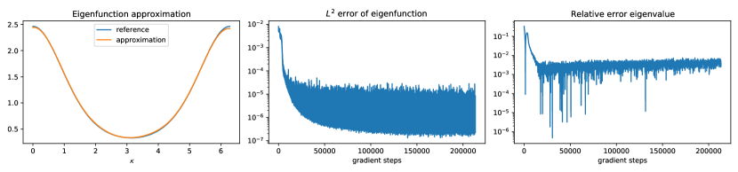
Figure 11: Left: Approximation and reference of the eigenfunction corresponding to the principal eigenvalue of the nonlinear Schrödinger operator in $d=5$. Middle: $L^{2}$ error w.r.t. test data along the training iterations. Right: Relative error of the approximated eigenvalue along the gradient steps.

We repeat the experiment in dimension $d=10$ and display the results in Figure 12. The optimization task gets slightly more difficult, but the resulting eigenfunction and eigenvalue still fit the reference solution reasonably well. Note that in both experiments no explicit boundary conditions, but only the norm constraint and the periodicity are imposed.

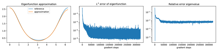
Figure 12: Same experiment as in Figure 11 in dimension $d=10$.

7 Conclusion and Outlook

In this paper, we have investigated the relationship between BSDE and PINN based approximation schemes for high-dimensional PDEs through the lens of the novel diffusion loss. In particular, we have shown that the diffusion loss provides an interpolation between the aforementioned methods and demonstrated its promising numerical performance in a range of experiments, allowing us to trade-off strengths and weaknesses of BSDEs and PINNs. Although we believe that the diffusion loss may be a stepping stone towards a unified understanding of computational approaches for high-dimensional PDEs, many questions remain open: First, there is a need for principled insights into the mechanisms with which BSDE, PINN and diffusion losses can or cannot overcome the curse of dimensionality. Second, it is of great practical interest to optimize the algorithmic details, preferably according to well-understood theoretical foundations. In this regard, we mention sophisticated (possibly adaptive) choices of the weights $\alpha_{\text{int}}$, $\alpha_{\text{b}}$, $\alpha_{\text{T}}$ and the measures $\nu_{\Omega\times[0,T]}$, $\nu_{\Omega}$, $\nu_{\partial\Omega\times[0,T]}$ as well as variance reduction techniques for estimator versions of the losses (see, for instance, [62, Remark 4.7]). Last but not least, we expect that the concepts explored in this paper may be fruitfully extended to the setting of parameter-dependent PDEs.

Acknowledgements. This research has been funded by Deutsche Forschungsgemeinschaft (DFG) through the grant CRC 1114 ‘Scaling Cascades in Complex Systems’ (projects A02 and A05, project number 235221301). We would like to thank Carsten Hartmann for many useful discussions.

References

- [1] William F Ames “Numerical methods for partial differential equations” Academic press, 2014
- [2] Francis Bach “Breaking the curse of dimensionality with convex neural networks” In The Journal of Machine Learning Research 18.1 JMLR. org, 2017, pp. 629–681
- [3] Christian Beck et al. “Deep splitting method for parabolic PDEs” In SIAM Journal on Scientific Computing 43.5 SIAM, 2021, pp. A3135–A3154
- [4] Christian Beck et al. “Solving stochastic differential equations and Kolmogorov equations by means of deep learning” In arXiv:1806.00421, 2018
- [5] Christian Beck, Weinan E and Arnulf Jentzen “Machine learning approximation algorithms for high-dimensional fully nonlinear partial differential equations and second-order backward stochastic differential equations” In Journal of Nonlinear Science 29.4 Springer, 2019, pp. 1563–1619
- [6] Christian Beck, Martin Hutzenthaler, Arnulf Jentzen and Benno Kuckuck “An overview on deep learning-based approximation methods for partial differential equations” In arXiv preprint arXiv:2012.12348, 2020
- [7] Sebastian Becker et al. “Numerical simulations for full history recursive multilevel Picard approximations for systems of high-dimensional partial differential equations” In arXiv preprint arXiv:2005.10206, 2020
- [8] Henri Berestycki, Louis Nirenberg and SR Srinivasa Varadhan “The principal eigenvalue and maximum principle for second-order elliptic operators in general domains” In Communications on Pure and Applied Mathematics 47.1 Wiley Online Library, 1994, pp. 47–92
- [9] Jens Berg and Kaj Nyström “A unified deep artificial neural network approach to partial differential equations in complex geometries” In Neurocomputing 317 Elsevier, 2018, pp. 28–41
- [10] Julius Berner, Philipp Grohs and Arnulf Jentzen “Analysis of the Generalization Error: Empirical Risk Minimization over Deep Artificial Neural Networks Overcomes the Curse of Dimensionality in the Numerical Approximation of Black–Scholes Partial Differential Equations” In SIAM Journal on Mathematics of Data Science 2.3 SIAM, 2020, pp. 631–657
- [11] Jean-Michel Bismut “Conjugate convex functions in optimal stochastic control” In Journal of Mathematical Analysis and Applications 44.2 Academic Press, 1973, pp. 384–404
- [12] Jan Blechschmidt and Oliver G Ernst “Three ways to solve partial differential equations with neural networks—A review” In GAMM-Mitteilungen Wiley Online Library, 2021, pp. e202100006
- [13] Bruno Bouchard and Stephane Menozzi “Strong approximations of BSDEs in a domain” In Bernoulli 15.4 Bernoulli Society for Mathematical StatisticsProbability, 2009, pp. 1117–1147
- [14] Bruno Bouchard and Nizar Touzi “Discrete-time approximation and Monte-Carlo simulation of backward stochastic differential equations” In Stochastic Processes and their applications 111.2 Elsevier, 2004, pp. 175–206
- [15] FM Buchmann and WP Petersen “Solving Dirichlet problems numerically using the Feynman-Kac representation” In BIT Numerical Mathematics 43.3 Springer, 2003, pp. 519–540
- [16] Giuseppe Carleo and Matthias Troyer “Solving the quantum many-body problem with artificial neural networks” In Science 355.6325 American Association for the Advancement of Science, 2017, pp. 602–606
- [17] Tim De Ryck and Siddhartha Mishra “Error analysis for physics informed neural networks (PINNs) approximating Kolmogorov PDEs” In arXiv preprint arXiv:2106.14473, 2021
- [18] Tim Dockhorn “A discussion on solving partial differential equations using neural networks” In arXiv preprint arXiv:1904.07200, 2019
- [19] Weinan E, Jiequn Han and Arnulf Jentzen “Deep learning-based numerical methods for high-dimensional parabolic partial differential equations and backward stochastic differential equations” In Communications in Mathematics and Statistics 5.4 Springer, 2017, pp. 349–380
- [20] Weinan E, Jiequn Han and Arnulf Jentzen “Algorithms for solving high dimensional PDEs: From nonlinear Monte Carlo to machine learning” In arXiv preprint arXiv:2008.13333, 2020
- [21] Weinan E and Eric Vanden-Eijnden “Towards a theory of transition paths” In Journal of statistical physics 123.3 Springer, 2006, pp. 503–523
- [22] Weinan E and Bing Yu “The deep Ritz method: a deep learning-based numerical algorithm for solving variational problems” In Communications in Mathematics and Statistics 6.1 Springer, 2018, pp. 1–12
- [23] Emmanuel Gobet, Jean-Philippe Lemor and Xavier Warin “A regression-based Monte Carlo method to solve backward stochastic differential equations” In The Annals of Applied Probability 15.3 Institute of Mathematical Statistics, 2005, pp. 2172–2202
- [24] Philipp Grohs and Lukas Herrmann “Deep neural network approximation for high-dimensional elliptic PDEs with boundary conditions” In arXiv preprint arXiv:2007.05384, 2020
- [25] Philipp Grohs, Fabian Hornung, Arnulf Jentzen and Philippe Von Wurstemberger “A proof that artificial neural networks overcome the curse of dimensionality in the numerical approximation of Black-Scholes partial differential equations” In arXiv preprint arXiv:1809.02362, 2018
- [26] Philipp Grohs, Arnulf Jentzen and Diyora Salimova “Deep neural network approximations for Monte Carlo algorithms” In arXiv:1908.10828, 2019
- [27] Eugene P Gross “Structure of a quantized vortex in boson systems” In Il Nuovo Cimento (1955-1965) 20.3 Springer, 1961, pp. 454–477
- [28] Jiequn Han, Arnulf Jentzen and Weinan E “Solving high-dimensional partial differential equations using deep learning” In Proceedings of the National Academy of Sciences 115.34 National Acad Sciences, 2018, pp. 8505–8510
- [29] Jiequn Han and Jihao Long “Convergence of the deep BSDE method for coupled FBSDEs” In Probability, Uncertainty and Quantitative Risk 5.1 Springer, 2020, pp. 1–33
- [30] Jiequn Han, Jianfeng Lu and Mo Zhou “Solving high-dimensional eigenvalue problems using deep neural networks: A diffusion Monte Carlo like approach” In Journal of Computational Physics 423 Elsevier, 2020, pp. 109792
- [31] Jihun Han, Mihai Nica and Adam R Stinchcombe “A derivative-free method for solving elliptic partial differential equations with deep neural networks” In Journal of Computational Physics 419 Elsevier, 2020, pp. 109672
- [32] Carsten Hartmann, Omar Kebiri, Lara Neureither and Lorenz Richter “Variational approach to rare event simulation using least-squares regression” In Chaos: An Interdisciplinary Journal of Nonlinear Science 29.6 AIP Publishing LLC, 2019, pp. 063107
- [33] ERIKA Hausenblas “A numerical scheme using Itô excursions for simulating local time resp. stochastic differential equations with reflection” In Osaka journal of mathematics 36.1 Osaka UniversityOsaka City University, Departments of Mathematics, 1999, pp. 105–137
- [34] Jan Hermann, Zeno Schätzle and Frank Noé “Deep-neural-network solution of the electronic Schrödinger equation” In Nature Chemistry 12.10 Nature Publishing Group, 2020, pp. 891–897
- [35] Gao Huang, Zhuang Liu, Laurens Van Der Maaten and Kilian Q Weinberger “Densely connected convolutional networks” In Proceedings of the IEEE conference on computer vision and pattern recognition, 2017, pp. 4700–4708
- [36] Côme Huré, Huyên Pham and Xavier Warin “Deep backward schemes for high-dimensional nonlinear PDEs” In Mathematics of Computation 89.324, 2020, pp. 1547–1579
- [37] Martin Hutzenthaler et al. “Overcoming the curse of dimensionality in the numerical approximation of semilinear parabolic partial differential equations” In Proceedings of the Royal Society A 476.2244 The Royal Society Publishing, 2020, pp. 20190630
- [38] Martin Hutzenthaler, Arnulf Jentzen, Thomas Kruse and Tuan Anh Nguyen “A proof that rectified deep neural networks overcome the curse of dimensionality in the numerical approximation of semilinear heat equations” In SN partial differential equations and applications 1.2 Springer, 2020, pp. 1–34
- [39] Martin Hutzenthaler, Arnulf Jentzen and Thomas Kruse “Multilevel Picard iterations for solving smooth semilinear parabolic heat equations” In arXiv preprint arXiv:1607.03295, 2016
- [40] Ameya D Jagtap, Kenji Kawaguchi and George Em Karniadakis “Adaptive activation functions accelerate convergence in deep and physics-informed neural networks” In Journal of Computational Physics 404 Elsevier, 2020, pp. 109136
- [41] Arnulf Jentzen, Diyora Salimova and Timo Welti “Proof that deep artificial neural networks overcome the curse of dimensionality in the numerical approximation of Kolmogorov partial differential equations with constant diffusion and nonlinear drift coefficients” In Communications in Mathematical Sciences 19.5 International Press of Boston, 2021, pp. 1167–1205
- [42] Li Jianyu, Luo Siwei, Qi Yingjian and Huang Yaping “Numerical solution of elliptic partial differential equation using radial basis function neural networks” In Neural Networks 16.5-6 Elsevier, 2003, pp. 729–734
- [43] Henry Jin, Marios Mattheakis and Pavlos Protopapas “Unsupervised Neural Networks for Quantum Eigenvalue Problems” In arXiv preprint arXiv:2010.05075, 2020
- [44] George Em Karniadakis et al. “Physics-informed machine learning” In Nature Reviews Physics 3.6 Nature Publishing Group, 2021, pp. 422–440
- [45] Yuehaw Khoo, Jianfeng Lu and Lexing Ying “Solving for high-dimensional committor functions using artificial neural networks” In Research in the Mathematical Sciences 6.1 Springer, 2019, pp. 1
- [46] Diederik P. Kingma and Jimmy Ba “Adam: A Method for Stochastic Optimization” In 3rd International Conference on Learning Representations, ICLR 2015, San Diego, CA, USA, May 7-9, 2015, Conference Track Proceedings, 2015 URL: http://arxiv.org/abs/1412.6980
- [47] Peter E Kloeden and Eckhard Platen “Stochastic differential equations” In Numerical Solution of Stochastic Differential Equations Springer, 1992, pp. 103–160
- [48] Stefan Kremsner, Alexander Steinicke and Michaela Szölgyenyi “A deep neural network algorithm for semilinear elliptic PDEs with applications in insurance mathematics” In Risks 8.4 Multidisciplinary Digital Publishing Institute, 2020, pp. 136
- [49] Isaac E Lagaris, Aristidis Likas and Dimitrios I Fotiadis “Artificial neural network methods in quantum mechanics” In Computer Physics Communications 104.1-3 Elsevier, 1997, pp. 1–14
- [50] Isaac E Lagaris, Aristidis Likas and Dimitrios I Fotiadis “Artificial neural networks for solving ordinary and partial differential equations” In IEEE transactions on neural networks 9.5 IEEE, 1998, pp. 987–1000
- [51] Isaac E Lagaris, Aristidis C Likas and Dimitris G Papageorgiou “Neural-network methods for boundary value problems with irregular boundaries” In IEEE Transactions on Neural Networks 11.5 IEEE, 2000, pp. 1041–1049
- [52] Hyuk Lee and In Seok Kang “Neural algorithm for solving differential equations” In Journal of Computational Physics 91.1 Elsevier, 1990, pp. 110–131
- [53] Qianxiao Li, Bo Lin and Weiqing Ren “Computing committor functions for the study of rare events using deep learning” In The Journal of Chemical Physics 151.5 AIP Publishing LLC, 2019, pp. 054112
- [54] Zongyi Li et al. “Fourier neural operator for parametric partial differential equations” In arXiv preprint arXiv:2010.08895, 2020
- [55] Jianfeng Lu and Yulong Lu “A Priori Generalization Error Analysis of Two-Layer Neural Networks for Solving High Dimensional Schrödinger Eigenvalue Problems” In arXiv preprint arXiv:2105.01228, 2021
- [56] Jianfeng Lu and James Nolen “Reactive trajectories and the transition path process” In Probability Theory and Related Fields 161.1 Springer, 2015, pp. 195–244
- [57] Martin Magill, Faisal Qureshi and Hendrick W Haan “Neural networks trained to solve differential equations learn general representations” In arXiv preprint arXiv:1807.00042, 2018
- [58] Cameron Martin et al. “Solving elliptic equations with Brownian motion: bias reduction and temporal difference learning” In Methodology and Computing in Applied Probability 24.3 Springer, 2022, pp. 1603–1626
- [59] Siddhartha Mishra and Roberto Molinaro “Estimates on the generalization error of physics informed neural networks (PINNs) for approximating PDEs” In arXiv preprint arXiv:2006.16144, 2020
- [60] Johannes Müller and Marius Zeinhofer “Deep Ritz revisited” In arXiv preprint arXiv:1912.03937, 2019
- [61] Johannes Müller and Marius Zeinhofer “Notes on Exact Boundary Values in Residual Minimisation” In arXiv preprint arXiv:2105.02550, 2021
- [62] Nikolas Nüsken and Lorenz Richter “Solving high-dimensional Hamilton–Jacobi–Bellman PDEs using neural networks: perspectives from the theory of controlled diffusions and measures on path space” In SN Partial Differential Equations and Applications 2.4 Springer, 2021, pp. 1–48
- [63] Étienne Pardoux “Backward stochastic differential equations and viscosity solutions of systems of semilinear parabolic and elliptic PDEs of second order” In Stochastic Analysis and Related Topics VI Springer, 1998, pp. 79–127
- [64] Etienne Pardoux and Shige Peng “Adapted solution of a backward stochastic differential equation” In Systems & Control Letters 14.1 Elsevier, 1990, pp. 55–61
- [65] Étienne Pardoux and Shuguang Zhang “Generalized BSDEs and nonlinear Neumann boundary value problems” In Probability Theory and Related Fields 110.4 Springer, 1998, pp. 535–558
- [66] Grigorios A Pavliotis “Stochastic processes and applications: diffusion processes, the Fokker-Planck and Langevin equations” Springer, 2014
- [67] David Pfau, James S Spencer, Alexander GDG Matthews and W Matthew C Foulkes “Ab initio solution of the many-electron Schrödinger equation with deep neural networks” In Physical Review Research 2.3 APS, 2020, pp. 033429
- [68] Huyên Pham “Continuous-time stochastic control and optimization with financial applications” Springer Science & Business Media, 2009
- [69] Lev P Pitaevskii “Vortex lines in an imperfect Bose gas” In Sov. Phys. JETP 13.2, 1961, pp. 451–454
- [70] Maziar Raissi “Forward-backward stochastic neural networks: Deep learning of high-dimensional partial differential equations” In arXiv preprint arXiv:1804.07010, 2018
- [71] Maziar Raissi, Paris Perdikaris and George E Karniadakis “Physics-informed neural networks: A deep learning framework for solving forward and inverse problems involving nonlinear partial differential equations” In Journal of Computational Physics 378 Elsevier, 2019, pp. 686–707
- [72] Maziar Raissi, Paris Perdikaris and George Em Karniadakis “Physics informed deep learning (part I): Data-driven solutions of nonlinear partial differential equations” In arXiv preprint arXiv:1711.10561, 2017
- [73] Lorenz Richter “Solving high-dimensional PDEs, approximation of path space measures and importance sampling of diffusions”, 2021
- [74] Lorenz Richter and Julius Berner “Robust SDE-based variational formulations for solving linear PDEs via deep learning” In International Conference on Machine Learning, 2022, pp. 18649–18666 PMLR
- [75] Lorenz Richter, Leon Sallandt and Nikolas Nüsken “Solving high-dimensional parabolic PDEs using the tensor train format” In Proceedings of the 38th International Conference on Machine Learning, ICML 2021, 18-24 July 2021, Virtual Event 139, Proceedings of Machine Learning Research PMLR, 2021, pp. 8998–9009 URL: http://proceedings.mlr.press/v139/richter21a.html
- [76] Grant M Rotskoff and Eric Vanden-Eijnden “Learning with rare data: Using active importance sampling to optimize objectives dominated by rare events” In arXiv preprint arXiv:2008.06334, 2020
- [77] Justin Sirignano and Konstantinos Spiliopoulos “DGM: A deep learning algorithm for solving partial differential equations” In Journal of computational physics 375 Elsevier, 2018, pp. 1339–1364
- [78] Csaba Szepesvári “Algorithms for reinforcement learning” In Synthesis lectures on artificial intelligence and machine learning 4.1 Morgan & Claypool Publishers, 2010, pp. 1–103
- [79] Tadasu Uchiyama and Noboru Sonehara “Solving inverse problems in nonlinear PDEs by recurrent neural networks” In IEEE International Conference on Neural Networks, 1993, pp. 99–102 IEEE
- [80] Remco Meer, Cornelis Oosterlee and Anastasia Borovykh “Optimally weighted loss functions for solving PDEs with Neural Networks” In arXiv preprint arXiv:2002.06269, 2020
- [81] Sifan Wang, Yujun Teng and Paris Perdikaris “Understanding and mitigating gradient flow pathologies in physics-informed neural networks” In SIAM Journal on Scientific Computing 43.5 SIAM, 2021, pp. A3055–A3081
- [82] Sifan Wang, Hanwen Wang and Paris Perdikaris “On the eigenvector bias of Fourier feature networks: From regression to solving multi-scale PDEs with physics-informed neural networks” In Computer Methods in Applied Mechanics and Engineering 384 Elsevier, 2021, pp. 113938
- [83] Sifan Wang, Xinling Yu and Paris Perdikaris “When and why PINNs fail to train: A neural tangent kernel perspective” In Journal of Computational Physics 449 Elsevier, 2022, pp. 110768
- [84] Yaohua Zang, Gang Bao, Xiaojing Ye and Haomin Zhou “Weak adversarial networks for high-dimensional partial differential equations” In Journal of Computational Physics 411 Elsevier, 2020, pp. 109409
- [85] Jianfeng Zhang “Backward stochastic differential equations” In Backward Stochastic Differential Equations Springer, 2017
- [86] Wei Zhang, Tiejun Li and Christof Schütte “Solving eigenvalue PDEs of metastable diffusion processes using artificial neural networks” In arXiv preprint arXiv:2110.14523, 2021
- [87] Mo Zhou, Jiequn Han and Jianfeng Lu “Actor-critic method for high dimensional static Hamilton–Jacobi–Bellman partial differential equations based on neural networks” In SIAM Journal on Scientific Computing 43.6 SIAM, 2021, pp. A4043–A4066