SalFBNet: Learning Pseudo-Saliency Distribution via Feedback Convolutional Networks

Abstract

Feed-forward only convolutional neural networks (CNNs) may ignore intrinsic relationships and potential benefits of feedback connections in vision tasks such as saliency detection, despite their significant representation capabilities. In this work, we propose a feedback-recursive convolutional framework (SalFBNet) for saliency detection. The proposed feedback model can learn abundant contextual representations by bridging a recursive pathway from higher-level feature blocks to low-level layers. Moreover, we create a large-scale Pseudo-Saliency dataset to alleviate the problem of data deficiency in saliency detection. We first use the proposed feedback model to learn saliency distribution from pseudo-ground-truth. Afterwards, we fine-tune the feedback model on existing eye-fixation datasets. Furthermore, we present a novel Selective Fixation and Non-Fixation Error (sFNE) loss to facilitate the proposed feedback model to better learn distinguishable eye-fixation-based features. Extensive experimental results show that our SalFBNet with fewer parameters achieves competitive results on the public saliency detection benchmarks, which demonstrate the effectiveness of proposed feedback model and Pseudo-Saliency data.

1 Introduction

Attention mechanism plays an important role in human visual system (HVS) by automatically focusing on the most relevant regions of observed scenes [1]. To better understand the attention mechanism of HVS, researchers often study human eye movement by recording a subject’s gaze while observing a stimuli (e.g. an image) [2], as shown in Figure 1 (a). In this way, the fixations collected from eye-tracker indicate the most attractive locations of a scene. Typically, saliency dense map is generated from fixation maps with a Gaussian kernel to further represent the salient locations. This pixel-wise dense map denotes the attentive regions of the stimuli [2] (see Figure 1 (a)). Saliency detection aims to find out the most informative and conspicuous fixations from a visual scene by simulating the similar attention mechanism of human eyes [3]. Saliency prediction on images/videos has been explored extensively in the past decades [2]. Fixation maps (fixation-based) collected from subjects and saliency maps (distribution-based) generated by the fixation maps are both regarded as the ground-truths (GTs) and used in the training and evaluation of saliency detection models [2, 3], as illustrated in Figure 1 (c).

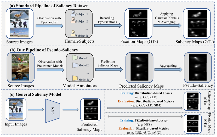
Figure 1: Pipelines of saliency annotation and general training/testing of saliency model. (a) Standard pipeline of eye-fixation dataset; (b) Our pipeline of pseudo saliency; (c) General training and testing of saliency models.

Saliency detection has been successfully applied to various computer vision tasks, such as compression [4] and image cropping [5]. Although great progress has been made in the field, there are still various challenges exist to be investigated and addressed. First, most existing CNN-based saliency models mainly utilize forward-only pathway to learn visual representations [3, 6], which ignores top-down connections of contextual features. In addition, some CNN-based saliency methods [7] employ large model size with high computational cost to improve representation learning capability. Moreover, the lack of manually-labeled annotations may hinder further performance boosts of existing models. However, the collection and annotation of human gaze from eye-tracker task is extremely time-consuming and labor-intensive.

To address the problem of insufficient training data for saliency prediction, we propose a similar pipeline of pseudo-saliency labelling motivated by the standard subjective experiments [2, 8] of human gaze collection from eye-tracker, as demonstrated in Figure 1 (b). In our pipeline, we use pre-trained CNN models to annotate saliency distribution of new RGB images. The well-known knowledge distillation (KD) method usually adopts teacher-student strategy to transfer softened knowledge from a large teacher network to a simple student model [9]. Inspired by knowledge distillation models, we believe that the saliency distribution knowledge learned from these pre-trained models can be transferred into pseudo-saliency annotations of new scenes. In this way, we can freely annotate saliency distribution of RGB images. These images and corresponding pseudo-annotations can be used for the training of saliency models.

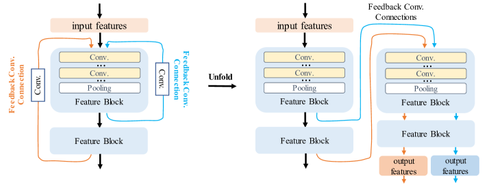
Figure 2: Simplified demonstration of feedback convolutional connections with two feature blocks.

In biology, feedback mechanism is usually used to maintain the balance of the system by amplifying or suppressing the feedback signal (e.g. positive or negative signal) [10]. Likewise, human brain and visual system also leverage feedback mechanisms to process complex cognitive behaviors [11]. Feedback convolutional networks have been introduced to learn abundant representations to mimic the feedback mechanism in various computer vision tasks [11, 12]. In our previous work [13], we explore an extremely lightweight feedback recursive model by linking the feature pathway from high-level blocks to low-level layer for saliency detection.

In this paper, we propose various model-based and experimental extensions to our previous work [13]. The contributions can be summarized as:

• First, we extend our previous work [13] in various ways: i) To be a more general framework, the encoder of the proposed model can be flexibly substituted by different popular backbones, such as ResNet [14], DenseNet [15], etc. ii) To achieve that, we adopt feedback convolutional connections to bridge the pathway of top-down representations, as shown in Figure 2. iii) Further, we utilize a new decoder with smoothing module as in [16] to incorporate the informative saliency scores from both forward- and feedback-streams.

• Second, we investigate the use of pseudo annotations for the training of proposed feedback framework. We found that the feedback models can learn rich representations from human-free annotated data, which demonstrates that the knowledge of saliency distribution can be transferred by model-annotators. Also, we compare the performance boost of different initialization ways for saliency prediction.

• Furthermore, we propose a novel Selective Fixation and Non-Fixation Error (sFNE) loss to make the proposed model better at learning eye-fixation-based features. Our sFNE loss not only considers the cost at fixation points, but also calculates the error at randomly selected non-fixation points.

Extensive experiments show the effectiveness of the proposed feedback framework and sFNE loss. Besides, we show that the feedback models can learn the information of saliency distribution from pseudo-saliency annotations.

2 Related Works

2.1 Saliency Detection on RGB Images

Saliency detection research is mainly classified into human eye fixation prediction (i.e. saliency map prediction) [2] and salient object detection (SOD) [17, 18]. Eye fixation prediction focuses on predicting human gazes on images where human eyes are most attracted to [2]. On the other hand, SOD aims to identify the regions of salient objects from an image [17, 18]. In this work, we focus on the prediction of human gaze from visual stimulus.

In the early ages, traditional saliency detection methods are usually developed based on bottom-up manner [1]. Recently, deep-learning based saliency methods [6, 19, 16] have achieved high performance through the superior capability of CNNs in feature representation. For example, Pan et al. introduce a generative adversarial model for visual saliency prediction [20]. Cornia et al. develop a CNN model to combine the multi-layer features for saliency detection [21]. Kummerer et al. propose a saliency detection model to explore the influence of low-level features (local intensity and contrast) and high-level features for eye-fixation prediction [22]. Droste et al. propose an unified saliency model based on domain adaptive for static images and dynamic videos [16]. Kroner et al. use a Atrous Spatial Pyramid Pooling (ASPP) module to capture multi-scale convolutional features for saliency detection [23]. Jia et al. establish an encoder-decoder-style network with expandable multi-layer for saliency prediction [24]. Fan et al. utilize a context adaptive saliency network to learn the spatial and semantic context for gaze prediction [25]. These models leverage a feed-forward-only architecture for saliency prediction, which may neglect the significant benefits of top-down features from feedback connection. In this work, we adopt feedback convolutional connections to bridge the feature pathway from high-level blocks to low-level layers to improve the representation ability.

2.2 Pseudo Labelling for Saliency Detection

The problem of insufficient training data in saliency detection urges the emergence of several previous works to reduce the dependency of human annotated ground-truths [17, 18, 2]. In the field of salient object detection (SOD), Nguyen et al. propose a self-supervised CNN model with conditional random field (CRF) to refine the noisy pseudo-labels generated from several handcrafted methods [26]. Different from the study [26], Zhang et al. propose a joint learning strategy for salient object detection and noise modelling [17]. Their hypothesis is that the pseudo-label of the input image can be represented as a combination of predicted saliency map and the noise map [17]. In the study [18], Zhang et al. propose a deep saliency model by learning the synthesized weak-supervision generated by unsupervised salient object detectors. It is mentioned in the study [27] that the backbone initialized by pre-trained weights on ImageNet [28] is not necessary for salient object detection (SOD). The authors state that saliency models require far fewer parameters than the classification approach [27]. In this work, we have reported similar findings in the field of eye fixation prediction.

However, to the best of our knowledge, there are a few works to address the problem of insufficient eye-fixation data due to the time-consuming gaze collection. Che et al. explore the influence of different distortions on gaze prediction [2]. They adopt several transformations, such as cropping/rotation, to augment existing saliency datasets (e.g. SALICON [29]). Then they collect eye-fixations of distorted image from eye tracker [2]. Although this method [2] augments SALICON [29], they still need to collect eye fixations from labor-intensive annotations. Besides, their method [2] does not provide data diversity from new visual scenes. Motivated by the standard subjective experiment of gaze collection, we annotate pseudo-labels by using pre-trained saliency models in this work.

2.3 Feedback Convolutional Networks

In recent years, feedback convolutional networks have been explored to learn top-down features in various computer vision applications [11, 12, 30, 31]. For example, Zamir et al. propose a feedback network based on convolutional LSTM for object recognition task [11]. They demonstrate that the feedback architecture can learn considerably different representations compared to the feed-forward counterpart [11]. Cao et al. establish a feedback convolutional model to learn top-down attentive visual features for image classification and recognition [12]. Stollenga et al. use feedback connections for deep selective attention networks to improve the performance of classification [32]. Li et al. propose to refine the low-level representation with high-level information by using a feedback convolutional network to improve the performance of image super-resolution [30]. Deng et al. introduce a deep-coupled feedback network for image exposure and super-resolution [31]. They use a multi-task learning strategy to optimize their feedback model [31]. In our previous work [13], we propose a lightweight feedback recursive network for image saliency prediction[13]. The works of [11, 12, 32] show that feedback convolutional network can learn rich representations for various vision tasks.

3 Proposed Method

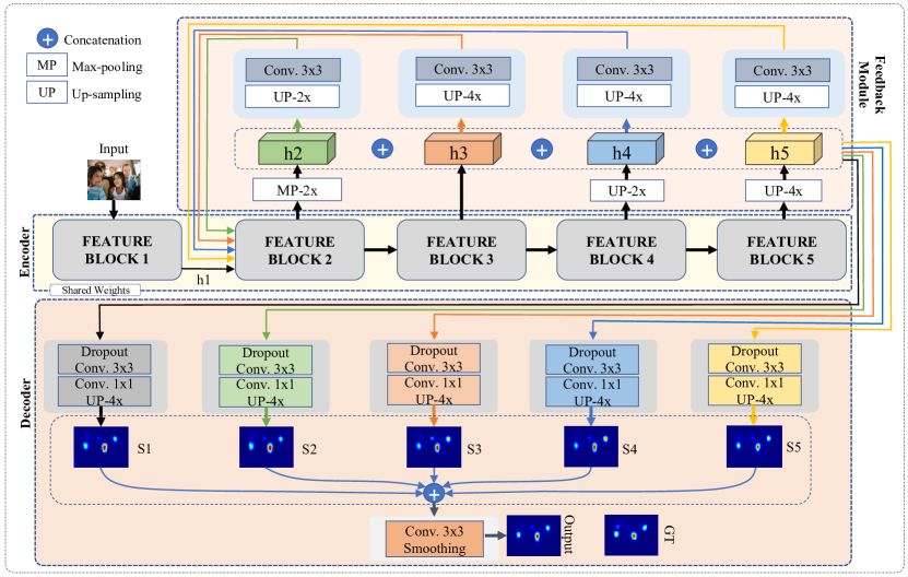
Figure 3: General architecture of proposed feedback convolutional network.

3.1 Feed-Forward Feature Learning

First, we build a feed-forward feature extractor with five CNN blocks to learn multi-scale representations from input images, as depicted in Figure 3. The encoder of the proposed model can be flexibly substituted by popular CNN backbones, such as ResNet [14], VGG [33], or DenseNet [15] (see Section 4.3.2). Afterwards, we fuse the multi-scale features {h2, h3, h4, h5} from all the other four CNN blocks. Then, the combined features are fed into the saliency decoder module to obtain the saliency score map (S1) of the forward pass. Finally, we calculate the loss between S1 and eye-fixation ground-truth.

3.2 Feature Feedback Module

Next, we feed back the learned multi-scale features from high-level CNN blocks to low-level convolutional layers with shared CNN parameters. To this end, our intuitive objective is to enable the network to recursively aggregate contextual information into a holistic description through feedback connections. Since the first block includes the input layer of color images, we select the first layer of the second CNN block as the input layer of feedback convolutional features, as shown in Figure 3.

We first extract the forward-feature h2 from feature block 2. After that, the h2 is fed back to the feed-forward feature extractor with a convolutional feedback connection and shared CNN weights. The feedback connection consists of an up-sampling layer and a convolutional layer with $3\times 3$ kernel. Thus, we can obtain the multi-scale feedback features (see the green arrows in Figure 3). The output feedback features $\hat{h}_{k}^{l}$ of $l$-th ($l\in\{2,3,4,5\}$) CNN block from $k$-th ($k\in\{2,3,4,5\}$) forward feature can be formulated as follows:

$$\hat{h}_{k}^{l}=f_{k}^{l}(\varphi(UP({h}_{k})*{W}_{k}^{fb}))$$ (1)

where ${W}_{k}^{fb}$ is the convolutional weights of $k$-th feedback connection; $h_{k}$ is the feed-forward feature of $k$-th CNN block; $*$ denotes the convolutional operation; the $UP$, $\varphi$, and $f_{k}^{l}$ represent the up-sampling, activation function, and the $l$-th convolutional block of $k$-th forward feature, respectively. Similar with the forward saliency head of the decoder, the saliency score S2 is predicted with feedback saliency head by using the feedback features $\hat{h}_{k}^{2}$.

Following the process in utilizing the forward feature h2, the forward feature h3 (orange arrows) from block 3, the forward feature h4 (blue arrows) from block 4, and the forward feature h5 (yellow arrows) from block 5 are also recursively fed back to the feed-forward feature extractor using feedback connections and the shared CNN weights, according to Equation 1. Hence, we obtain the enhanced informative feedback features $\hat{h}_{k}^{l}$ for each feed-forward feature ${h}_{k}$. Finally, the learned feedback features $\hat{h}_{k}^{l}$ are concatenated and passed to saliency heads of decoder for predicting the saliency scores S3, S4, and S5.

3.3 Saliency Feature Decoder

In the proposed feedback model, we utilize a feature decoder to aggregate the saliency scores from both forward and feedback pathways, as shown in Figure 3. The concatenated multi-scale features are used to predict the saliency score with individual saliency head in the decoder. The saliency scores $\{S_{n}|n\in\{1,2,3,4,5\}\}$ can be represented as:

$$S_{n}=UP(\varphi(\varphi(Dropout(H_{n})*{W}_{n}^{3\times 3})*{W}_{n}^{1\times 1})))$$ (2)

where $H_{n}$ denotes the fused features from encoder; ${W}_{n}^{3\times 3}$ and ${W}_{n}^{1\times 1}$ indicate the convolutional weights with $3\times 3$ and $1\times 1$ kernels for $n$-th saliency score, respectively; $Dropout$ is a dropout layer. Note that if $n=1$, the saliency score $S1$ is predicted by the forward pathway; otherwise, the saliency score is calculated by the feedback feature.

Next, we concatenate the informative saliency scores $S_{n}$ from a forward saliency head and four feedback saliency heads, as illustrated in Figure 3. Furthermore, we predict a final saliency map $\hat{\mathbf{S}}$ by using a fusion convolutional layer with $1\times 1$ kernel and a smoothing convolutional layer with $41\times 41$ kernel, which can be formulated as follows:

$$\hat{\mathbf{S}}=\varphi(Cat[S_{n}]*{W}^{fusion})*{W}^{smoothing}$$ (3)

where $n\in\{1,2,3,4,5\}$ denotes the indices of saliency scores; $Cat[~{}]$ is the concatenation operation; ${W}^{fusion}$ and ${W}^{smoothing}$ represent the convolutional weights of fusion and smoothing layer, respectively.

3.4 Loss Function

As stated in [34], normalized scanpath saliency (NSS) metric is often used to measure performance of a saliency model. NSS is generally calculated by averaging normalized saliency values at eye-fixation pixels. Typically, the higher the NSS value, the better the performance of a model. Thus, there are several works [4, 16] adopt negative NSS (i.e. -NSS) as loss function to train saliency models. However, the loss function of -NSS only considers the cost of normalized saliency at salient fixations, while ignoring the loss at non-salient fixations.

Inspired by NSS metric and variant NSS loss in the studies [24, 16], we introduce a novel fixation-based loss referred as Selective Fixation and Non-Fixation Error (sFNE) for training proposed feedback saliency model. We first randomly select the same number of non-fixations based on the fixations in the ground-truth map to ensure the balance between positive and negative samples in a normalized saliency map, as demonstrated in Figure 4. Our key idea is that the distribution between normalized prediction and ground-truth saliency map at both fixation and non-fixation locations should be as close as possible. To this end, we use sFNE to measure the difference of saliency distribution. Let $P,G,F,\bar{F}$ denote predicted saliency map, ground-truth saliency map, ground-truth fixation map, and selected non-fixation map, respectively. After normalization, we obtain normalized prediction $P^{\prime}$ and normalized label $G^{\prime}$. Then, the loss of fixation and non-fixation locations can be computed as:

$$\mathcal{L}_{fixation}=\frac{1}{N}\sum_{i=1}^{N}\|P^{\prime}_{i}\times F_{i}-G^{\prime}_{i}\times F_{i}\|^{2}$$ (4)

$$\mathcal{L}_{nonfixation}=\frac{1}{N}\sum_{j=1}^{N}\|P^{\prime}_{j}\times\bar{F}_{j}-G^{\prime}_{j}\times\bar{F}_{j}\|^{2}$$ (5)

where $F_{i}\in\{0,1\}$ and $\bar{F}_{j}\in\{0,1\}$; $N$ denotes the number of fixations, which can be written as:

$$N=\sum_{i}F_{i}=\sum_{j}\bar{F}_{j}$$ (6)

where $i,j$ represent the indices of fixation and non-fixations, respectively. Therefore, sFNE loss $\mathcal{L}_{sFNE}$ can be formulated as follows:

$$\mathcal{L}_{sFNE}=\alpha\mathcal{L}_{fixation}+\beta\mathcal{L}_{nonfixation}$$ (7)

where $\alpha,\beta$ are the weights of the fixation and non-fixation costs, respectively.

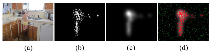
Figure 4: Illustration of Selective Fixation and Non-Fixation Error (sFNE) loss. From left to right: (a) image, (b) ground-truth fixation map, (c) ground-truth saliency map, (d) visualization of fixations (red points) in (b) and randomly-selected non-fixations (green points).

In addition to the fixation-based sFNE loss, we also combine other popular distribution-based loss [35, 4] in the field of saliency detection. In this work, we combine our sFNE loss with Correlation Coefficient (CC) loss and Kullback-Leibler Divergence (KLD) loss (see [36, 24] for formulations). Therefore, the combined loss of proposed feedback model can be represented as follows:

$$\mathcal{L}=\gamma\mathcal{L}_{KLD}+\delta\mathcal{L}_{CC}+\eta\mathcal{L}_{sFNE}$$ (8)

where $\gamma,\delta,\eta$ are the weighting constants of the three losses, respectively. Note that we utilize the $\mathcal{L}_{CC}=1-CC$ as CC loss to avoid the negative value.

Besides, we propose to deeply supervise the saliency scores from forward and feedback pathways with ground-truths. In this way, the proposed model can learn abundant enhanced multi-scale features for saliency prediction. More specifically, the total loss of the $n$ predicted saliency scores $\{S_{n},n\in\{1,2,3,4,5\}\}$ (i.e. saliency maps of the forward saliency head and four feedback saliency heads) can be represented as follows:

$$Loss_{score}=\frac{1}{N}\sum\mathcal{L}(S_{n},G,F,\bar{F})$$ (9)

where $n$ and $N$ are the index and number of the predicted saliency score, respectively. Finally, we measure the cost between the final fused saliency prediction $\hat{\mathbf{S}}$ and ground truth map by the following function:

$$Loss_{fuse}=\mathcal{L}(\hat{\mathbf{S}},G,F,\bar{F})$$ (10)

Thus, the overall loss for optimizing the proposed feedback saliency model can be calculated as:

$$Loss=\lambda_{1}Loss_{score}+\lambda_{2}Loss_{fuse}$$ (11)

where the hyper-parameters $\lambda_{1},\lambda_{2}$ are used for weighting the losses.

3.5 Saliency Knowledge Transferring

Motivated by the teacher-student strategy, we postulate that existing state-of-the-art pre-trained saliency models may have better initial knowledge of saliency distribution. Therefore, we conducted experiments to see if they can serve as better transmitters for transferring saliency knowledge to a new simple student model. To achieve this, starting with a set of images $\mathcal{X}=\{x_{i},i=1,...,N\}$, where $N$ is the number of images, we select arguably top five models from the benchmark lists of state-of-of-the-art methods in public databases. Then we use these $M$=5 pre-trained models to annotate the images $\mathcal{X}$. Similar with the standard subjective experiment of eye-fixation collection, we leverage these $M$ pre-trained models to generate the saliency probability maps $\mathcal{S}$ = $\{s_{i}^{j},i=1,...,N;j=1,...,M\}$, where $s_{i}^{j}$ denotes the predicted probability map of $i$-th image with $j$-th pre-trained model-annotator. In standard human gaze experiment, the ground-truth saliency map is calculated by recorded fixations with a Gaussian kernel to represent the saliency probability. However, since the pre-trained saliency model naturally predicts saliency probability of an input image, we directly aggregate the predictions of the pre-trained model-annotators to avoid the biases from various models. Specifically, the aggregated saliency map can be formulated as follows:

$${\bar{s}}_{i}=g(\sum_{j=1}^{M}\alpha{s}_{i}^{j})$$ (12)

where $\bar{s}_{i}$ denotes the aggregated prediction of the results from $M$ pre-trained models; $\alpha$ represents the weight for weighting the predicted distribution; $g$ is a normalization function. Here, $\alpha$=0.2 in this work. Thus, the assembled probability maps can be represented as $\mathcal{\bar{S}}=\{\bar{s}_{i},i=1,...,N\}$.

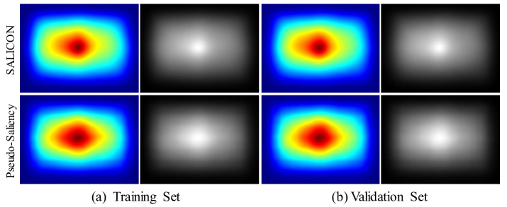
Figure 5: Illustration of saliency distribution. The top and bottom are averaged saliency distribution from SALICON [29] and our Pseudo-Saliency dataset, respectively.

To validate the aggregated pseudo-saliency probability map, we visualize the averaged saliency distribution and corresponding heat map on SALICON [29] in Figure 5. We observe that the pseudo-saliency distribution approximate to the distribution of human annotations. This validates our hypothesis that the saliency knowledge of the pre-trained models can be transferred to aggregated pseudo-labels. In this way, we can annotate the pseudo saliency of RGB image from any published datasets in a human-free manner. As proposed in this work, Pseudo-Saliency data can be an alternative way to train a new CNN model from scratch.

4 Experimental Results

4.1 Experimental Setup

In this work, we utilize six commonly-used saliency datasets, including SALICON [29], MIT1003 [37], MIT300 [8], DUT-OMRON [38], PASCAL-S [39], and TORONTO [40]. We show the detailed information of these datasets in Table 1. The large-scale SALICON [29] dataset officially contains training set, validation set, and testing set for saliency prediction. We randomly divide MIT1003 [37] into 900 images and 103 images for training set and validation set, respectively. After pre-training on Pesudo-Saliency dataset, we fine-tune our feedback models on SALICON [29] and MIT1003 [37]. Other datasets are used for performance testing, as illustrated in Table 1.

Table 1: Details of different saliency datasets.

Dataset	#Image	#Training	#Val.	#Testing	Size
MIT300 [8]	300	-	-	300	$\sim$ 44.4 MB
PASCAL-S [39]	850	-	-	850	$\sim$ 108.3 MB
DUT-OMRON [38]	5,168	-	-	5,168	$\sim$ 151.8 MB
TORONTO [40]	120	-	-	120	$\sim$ 92.3 MB
SALICON [29]	20,000	10,000	5,000	5,000	$\sim$ 4 GB
MIT1003 [37]	1003	900*	103*	-	$\sim$ 178.7 MB
Pseudo-Saliency (Ours)	176,880	150,000	26,880	-	$\sim$ 24.2 GB
*The training set and validation set are randomly split in this work.

The proposed feedback models are implemented with PyTorch library. We utilize SGD optimizer for optimization. Batch size, momentum and weight decay values are 10, 0.9 and 1e-4, respectively. The initial learning rates of pre-training and fine-tuning are 4e-2 and 1e-4, respectively. The learning rate decay value is set as 0.9. In our model, factor of dropout is 0.5 and activation function $\varphi$ is ReLU. In Equation (7) and (11), the weights of $\alpha,\beta,\lambda_{1},\lambda_{2}$ are set as 1. In Equation (8), we use $\gamma$=1, $\delta$=0.1, and $\eta$=0.025, respectively.

For pseudo-saliency annotation, we first select 150,000 color images from widely-used ImageNet [28] dataset and 26,880 color images from SOD datasets. In our experiment, SOD datasets include CSSD [41], ECSSD [42], HKU-IS[43], MSRA-B[44], MSRA10K[45], and THUR15K[46]. Afterwards, we choose M=5 pre-trained saliency models to annotate these images. The pre-trained models include DeepGazeIIE [19], UNISAL [16], MSINet [23], EMLNet [24], CASNetII [25]. We directly use their pre-trained weights and default settings for inference of saliency distribution. Therefore, we create a large-scale Pseudo-Saliency dataset containing 176,880 color images and corresponding pseudo-ground-truths. Our Pseudo-Saliency dataset is divided into training set and validation set, as shown in Table 1.

Similar with the studies [16, 34], we use popular metrics to report performance results, including linear correlation coefficient (CC), area under ROC curve (AUC), shuffled AUC (sAUC), normalized scanpath saliency (NSS), similarity (SIM), information gain (IG) and Kullback-Leibler divergence (KLdiv). Note that the larger the value of IG, CC, AUC, sAUC, and NSS, and the smaller the value of KLdiv, the better the performance of the saliency model (see the study [34] for more information about these metrics). For a fair comparison, we utilize same implementations of these metrics for performance evaluation.

4.2 Comparison with Existing Saliency Methods

In this experiment, we compare our feedback models with existing saliency prediction methods on 5 popular eye-fixation datasets, including SALICON [29], MIT300 [8], DUT-OMRON [38], PASCAL-S [39], and TORONTO [40].

Table 2: Quantitative comparison with 8 existing methods on SALICON [29] testing set. Pub. means the publication of the method. The best three results are respectively shown in red, blue, and green color.

Model	Pub.	AUC $\uparrow$	sAUC $\uparrow$	IG $\uparrow$	NSS $\uparrow$	CC $\uparrow$	SIM $\uparrow$	KLdiv $\downarrow$
MD-SEM [4]	CVPR2020	0.8640	0.7460	0.6600	2.0580	0.8680	0.7740	0.5680
EMLNet [24]	IVC2020	0.8660	0.7460	0.7360	2.0500	0.8860	0.7800	0.5200
SAM-Res [6]	TIP2018	0.8650	0.7410	0.5380	1.9900	0.8990	0.7930	0.6100
ACNet-V17 [47]	NC2021	0.8660	0.7390	0.8540	1.9480	0.8960	0.7860	0.2280
DI-Net [35]	TMM2019	0.8620	0.7390	0.1950	1.9590	0.9020	0.7950	0.8640
MSI-Net [23]	NN2020	0.8650	0.7360	0.7930	1.9310	0.8890	0.7840	0.3070
GazeGAN [2]	TIP2019	0.8640	0.7360	0.7200	1.8990	0.8790	0.7730	0.3760
FBNet [13]	MVA2021	0.8430	0.7060	0.3430	1.6870	0.7850	0.6940	0.7080
SalFBNet-Res18 (Ours)	-	0.8670	0.7330	0.8050	1.9500	0.8880	0.7730	0.3030
SalFBNet-Res18Fixed (Ours)	-	0.8680	0.7400	0.8390	1.9520	0.8920	0.7720	0.2360
Note that all the metric values are collected from the SALICON [29] leaderboard and the literature.

For SALICON [29] dataset, we evaluate the results of two feedback models: SalFBNet-Res18 and SalFBNet-Res18Fixed. The backbone of SalFBNet-Res18 is ResNet18 [14], while the backbone of SalFBNet-Res18Fixed is ResNet18 with fixed filter size of 128. After finetuning on SALICON [29], we submit our prediction results of the testing set to the official server of SALICON [29] for evaluation. We report the quantitative results of SALICON [29] in Table 2, including 8 existing saliency methods. We can see that our two feedback models rank in the top three for the most metrics and achieve competitive performances compared with the existing methods. Especially, the AUC value of SalFBNet-Res18Fixed achieves the best. Additionally, SalFBNet-Res18Fixed outperforms SalFBNet-Res18 on most metrics. These comparison results further verify the finding that the feedback model with few number of parameters can also learn rich representation for saliency prediction. Also, these two extended feedback models outperform our previous FBNet [13] model by a large margin. These results demonstrated the effectiveness of the feedback framework and our training scheme with pseudo-saliency data and sFNE loss.

Table 3: Quantitative comparison with 24 existing methods on MIT300 [8] testing set. D and T means the CNN-based and traditional-based method. Pub. means the publication of the method. The best three results are respectively shown in red, blue, and green color.

Model	Pub.	D/T	AUC $\uparrow$	sAUC $\uparrow$	NSS $\uparrow$	CC $\uparrow$	KLdiv $\downarrow$	SIM $\uparrow$
CovSal [48]	JoV2013	T	0.8116	0.5894	1.3362	0.5000	1.7220	0.5058
LDS [49]	TNNLS2016	T	0.8108	0.6020	1.3649	0.5177	1.0631	0.5222
Judd [37]	ICCV2009	T	0.8095	0.6003	1.1882	0.4664	1.1084	0.4182
GBVS [50]	NIPS2006	T	0.8062	0.6299	1.2457	0.4791	0.8878	0.4835
BMS [51]	ICCV2013	T	0.7718	0.6918	1.1512	0.4130	1.0235	0.4456
AIM [40]	JoV2007	T	0.7619	0.6647	0.8824	0.3419	1.2476	0.4096
CAS [52]	TPAMI2011	T	0.7581	0.6402	1.0186	0.3848	1.0723	0.4319
Itti98 [1]	TPAMI1998	T	0.5434	0.5357	0.4081	0.1307	1.4964	0.3378
CASNetII [25]	CVPR2018	D	0.8552	0.7398	1.9859	0.7054	0.5857	0.5806
SAM-Res [6]	TIP2018	D	0.8526	0.7396	2.0628	0.6897	1.1710	0.6122
SalGAN [20]	CVPRW2017	D	0.8498	0.7354	1.8620	0.6740	0.7574	0.5932
SAM-VGG [6]	TIP2018	D	0.8473	0.7305	1.9552	0.6630	1.2746	0.5986
DVA [3]	TIP2018	D	0.8430	0.7257	1.9305	0.6631	0.6293	0.5848
DeepGazeI [53]	ICLR2015	D	0.8427	0.7232	1.7234	0.6144	0.6678	0.5717
MLNet [54]	ICPR2016	D	0.8368	0.7399	1.9748	0.6633	0.8006	0.5819
ICF [22]	ICCV2017	D	0.8330	0.6957	1.6134	0.5876	0.7084	0.5576
eDN [55]	CVPR2014	D	0.8171	0.6180	1.1399	0.4518	1.1369	0.4112
SALICON [56]	ICCV2015	D	0.8171	0.6180	1.1399	0.4518	1.1369	0.4112
MSI-Net [23]	NN2020	D	0.8738	0.7787	2.3053	0.7790	0.4232	0.6704
DeepGazeII [22]	ICCV2017	D	0.8733	0.7759	2.3371	0.7703	0.4239	0.6636
GazeGAN [2]	TIP2019	D	0.8607	0.7316	2.2118	0.7579	1.3390	0.6491
EMLNet [24]	IVC2020	D	0.8762	0.7469	2.4876	0.7893	0.8439	0.6756
UNISAL [16]	ECCV2020	D	0.8772	0.7840	2.3689	0.7851	0.4149	0.6746
DeepGazeIIE [19]	ECCV2021	D	0.8829	0.7942	2.5265	0.8242	0.3474	0.6993
SalFBNet-Res18 (Ours)	-	D	0.8769	0.7858	2.4702	0.8141	0.4151	0.6933
Note that all the metric values are collected from the MIT300 [8] leaderboard.

Table 4: Quantitative comparison with 11 existing methods on testing sets of DUT-OMRON [38], PASCAL-S [39], and TORONTO [40]. The best three results are respectively shown in red, blue, and green color.

	Method	DUT-OMRON [38]						PASCAL-S [39]						TORONTO [40]
		AUC-J	AUC-B	sAUC	CC	NSS	SIM	AUC-J	AUC-B	sAUC	CC	NSS	SIM	AUC-J	AUC-B	sAUC	CC	NSS	SIM
Traditional	CAS [52]	0.8000	0.7900	0.7300	0.4000	1.4700	0.3700	0.7800	0.7500	0.6700	0.3600	1.1200	0.3400	0.7800	0.7800	0.6900	0.4500	1.2700	0.4400
	AIM [40]	0.7700	0.7500	0.6900	0.3000	1.0500	0.3200	0.7700	0.7500	0.6500	0.3200	0.9700	0.3000	0.7600	0.7500	0.6700	0.3000	0.8400	0.3600
	GBVS [50]	0.8700	0.8500	0.8100	0.5300	1.7100	0.4300	0.8400	0.8200	0.6500	0.4500	1.3600	0.3600	0.8300	0.8300	0.6400	0.5700	1.5200	0.4900
	Itti98 [1]	0.8300	0.8300	0.7800	0.4600	1.5400	0.3900	0.8200	0.8000	0.6400	0.4200	1.3000	0.3600	0.8000	0.8000	0.6500	0.4800	1.3000	0.4500
Deep-Learning-based	DVA [3]	0.9100	0.8600	0.8400	0.6700	3.0900	0.3900	0.8900	0.8600	0.7600	0.7200	2.1200	0.5800	0.8600	0.8600	0.7600	0.7200	2.1200	0.5800
	*MSI-Net [23]	0.9149	0.8947	0.8187	0.6613	2.9350	0.4920	0.8931	0.8541	0.7532	0.6603	2.2641	0.5264	0.8702	0.8263	0.7249	0.7419	2.1187	0.6253
	*DeepGazeIIE [22]	0.9044	0.8722	0.7647	0.6184	2.4690	0.4832	0.9125	0.8672	0.7338	0.7676	2.5401	0.6136	0.8805	0.8184	0.6964	0.8034	2.3019	0.6659
	*EMLNet [24]	0.9121	0.8628	0.8021	0.6620	3.1418	0.5281	0.8897	0.8249	0.7406	0.6636	2.3581	0.5464	0.8546	0.7818	0.6990	0.7291	2.1901	0.6142
	*CASNetII [25]	0.9003	0.8832	0.8024	0.6012	2.6105	0.4356	0.8856	0.8518	0.7473	0.6356	2.1741	0.4915	0.8629	0.8328	0.7175	0.6968	1.9447	0.5781
	*UNISAL [16]	0.8913	0.8413	0.7779	0.5577	2.7776	0.4235	0.8766	0.7997	0.7212	0.5763	2.0919	0.4766	0.8692	0.7785	0.7067	0.6965	2.2050	0.5953
	*FBNet [13]	0.9050	0.8928	0.8022	0.5848	2.5051	0.3959	0.8889	0.8685	0.7498	0.6121	2.0568	0.4540	0.8697	0.8467	0.7094	0.7141	1.9707	0.5759
Ours	SalFBNet-Res18	0.9118	0.8403	0.7740	0.6339	3.0879	0.4929	0.9043	0.7964	0.7155	0.6784	2.4997	0.5611	0.8794	0.7887	0.6942	0.7619	2.3314	0.6382
	SalFBNet-Res18Fixed	0.9144	0.8949	0.8179	0.6417	2.8716	0.4622	0.8943	0.8581	0.7523	0.6518	2.2429	0.5081	0.8756	0.8354	0.7264	0.7475	2.1340	0.6200
	$\dagger$SalFBNet-Res18	0.9269	0.8856	0.8145	0.7275	3.3439	0.5387	0.9072	0.8395	0.7434	0.7336	2.5808	0.5730	0.8824	0.8114	0.7015	0.8103	2.3647	0.6576
	$\dagger$SalFBNet-Res18Fixed	0.9250	0.8826	0.8092	0.7148	3.2755	0.5016	0.9060	0.8367	0.7382	0.7186	2.5271	0.5429	0.8782	0.8099	0.6948	0.7826	2.2666	0.6288
* denotes the results are generated by their source code with default settings. Others are collected from the study [3].
$\dagger$ denotes the model is finetuned on the mixture training set of Pseudo-Saliency (900 samples) and MIT1003 (900 samples).

For the evaluation of MIT300 [8] dataset, we first use MIT1003 [37] to fine-tune our feedback model, then submit our results to MIT300 [8] benchmark. In this work, we divide MIT1003 [37] into training set and validation set for fine-tuning, as shown in Table 1. We show the quantitative experimental results in Table 3 on MIT300 testing set, including 16 existing deep-learning-based and 8 traditional-based approaches over 6 commonly used evaluation metrics. Note that all metric values of Table 3 are collected from the benchmark leaderboard of MIT300. We can observe that the feedback model (SalFBNet-Res18) surpasses most existing saliency methods by a large margin. For example, the CC value and SIM value of our model achieve 0.8141 and 0.6933, respectively. For these two metrics, only our feedback model and DeepGazeIIE [19] obtain the performance of CC$\geq$0.81 and SIM$\geq$0.69. In addition, most metric values of our feedback model are ranked in the top three, and the performance gap between proposed model and the best model (DeepGazeIIE [19]) is very small (e.g. sAUC: 0.84%, CC: 1.01%, SIM: 0.6%).

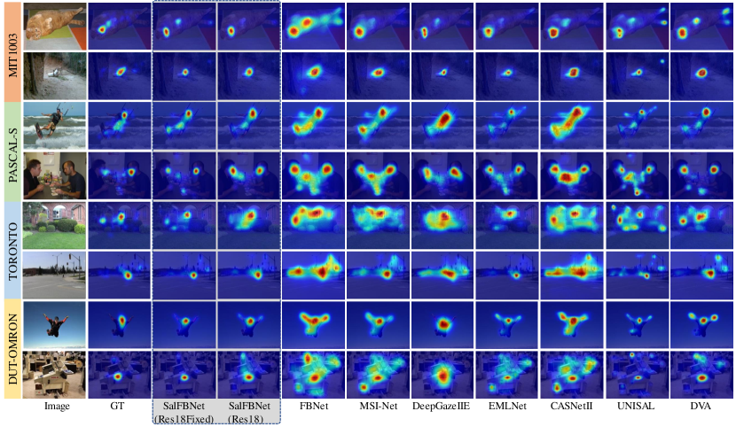
Figure 6: Visualization comparison on different datasets, including MIT1003 [37], PASCAL-S [39], TORONTO [40], and DUT-OMRON [38]. From left to right: Image, ground-truth (GT), SalFBNet-Res18Fixed128 (Ours), SalFBNet-Res18 (Ours), FBNet [13], MSI-Net [23], DeepGazeIIE [19], EMLNet [24], CASNetII [25], UNISAL [16], and DVA [3].

Moreover, we compare our feedback models with 11 existing saliency methods on other three popular benchmarks, including DUT-OMRON [38], PASCAL-S [39], and TORONTO [40]. These existing models contain 4 conventional-based methods and 7 deep-learning-based models. In Table 4, we show the quantitative comparison results. We first collect the available metric values from the study [3]. For other models, we use their released code for the inference of saliency prediction with the default settings. After that, we evaluate all models with the same evaluation implementation (see Section 4.1). In this experiment, we use a mixture training set with Pseudo-Saliency (900 samples) and MIT1003 (900 samples) for fine-tuning. From Table 4, we can find that our feedback models achieve competitive quantitative results on these three datasets. Our two feedback models are also ranked on the top three in most metrics. Besides, our previous extremely lightweight FBNet [13] achieves the second best performance in terms of AUC-B metric on TORONTO [40]. Furthermore, the feedback models finetuned with the mixture training set gain additional improvements and achieve the best performance. For instance, SalFBNet-Res18 achieves the best NSS performance on all three datasets after fine-tuning on the mixture training set. These results show that the performance can be further improved with the pseudo-saliency data. Finally, we visualize some challenging scenes and saliency predictions of different models in Figure 6. We can observe that our SalFBNet-Res18 and SalFBNet-Res18Fixed models can obtain better visual results in complex scenes compared with the state-of-the-art models.

4.3 Ablation Studies

In this section, we conduct extensive ablation studies to better understand the influence of various experimental settings in the proposed architecture.

Table 5: Quantitative performance of pseudo-annotators on SALICON [29] validation set. Pseudo-Saliency means the result of aggregated saliency prediction.

Metric	AUC-J $\uparrow$	AUC-B $\uparrow$	sAUC $\uparrow$	CC $\uparrow$	NSS $\uparrow$	KLdiv $\downarrow$	SIM $\uparrow$
MSINet [23]	0.8678	0.8332	0.7261	0.8886	1.9040	0.2752	0.7816
DeepGaze [19]	0.8559	0.7604	0.6572	0.7931	1.7258	0.5482	0.6927
EMLNet [24]	0.8665	0.7974	0.7129	0.8789	1.9924	0.7363	0.7691
CASNet [25]	0.8569	0.8283	0.7148	0.8416	1.7814	0.3523	0.7194
UNISAL [16]	0.8490	0.7656	0.6935	0.7710	1.8401	0.7479	0.6827
Pseudo-Saliency	0.8706	0.8315	0.7236	0.8961	1.9591	0.2555	0.7784

4.3.1 Analysis of Transferred Pseudo-Saliency

We first conduct experiments to evaluate the effectiveness of the pseudo-saliency knowledge transferred from model-annotators. We compare quantitative performance between Pseudo-Saliency and the five model-annotators on SALICON [29] validation set as shown in Table 5. In addition, we show several saliency prediction samples of different annotators in Figure 7. More detailed analysis on the selected saliency models and aggregated pseudo saliency results can be found in Figure 1 and Table 3 of Supplementary file. From these experiments, we verify the following observations:

i) All pseudo-annotators can predict roughly correct distribution by visually and quantitatively comparing with the ground-truth, but some predicted gazes are shifted and incomplete. For instance, the prediction of CASNetII [25] is shifted to the animal head in the third row of Figure 7.

Figure 7: Visualization results of different model-annotators. The results are collected from annotators including MSINet [23], DeepGazeIIE [19], EMLNet [24], CASNetII [25], and UNISAL [16]. PseudoSaliency means the aggregated pseudo-saliency in this work.

ii) These methods are able to predict similar saliency distributions. However, there are biases from different models due to various model settings and training strategies. Therefore, we aggregate predicted distributions of these models to alleviate deviations from different model-annotators.

iii) The aggregated pseudo-saliency not only combines the advantages of each annotator, but also suppresses some potential defective predictions. Quantitatively, the metric values of PseudoSaliency are always close to the best model among these model-annotators, and even achieve superior performance, such as AUC-J and KLdiv in Table 5.

4.3.2 Influences of backbones and training settings

We extend the feature extractor of the feedback model with different popular backbones to further demonstrate the flexibility, stability and consistency of the proposed framework, including ResNet [14], DenseNet [15]. We also modify a feedback model, namely Res18Fixed128, to compare with our previous work [13]. The backbone of Res18Fixed128 is ResNet18 [14] with fixed filter size of 128 in all convolution layers. In this work, we experimentally select 128 for the model with fixed filter size. The details and results of filter size selection experiments are given in Table 1 and Table 2 of Supplementary file. For training, we use different initialization settings to verify the pre-trained weights on ImageNet [28]. We first pre-train these feedback models on Pseudo-Saliency dataset without using any human annotated ground truth of public datasets. Extensive results with pre-trained performance of our proposed framework using various backbone models on SALICON [29] validation set are shown and compared in Table 4 of Supplementary file. We then finetune them on SALICON [29] with proposed loss in Equation (8). From Table 6, we can draw the following conclusions:

i) There is a slight influence between feedback models initialized by ImageNet [28] pre-trained weights and random initialization. In particular, the performance of some randomly initialized models even surpasses that of initialized by ImageNet [28] pre-trained weights.

Table 6: Comparison of finetuning performance of feedback models with different backbones and initialization strategies.

Backbone	Init.	Train	Eval.	AUC-J $\uparrow$	AUC-B $\uparrow$	sAUC $\uparrow$	CC $\uparrow$	NSS $\uparrow$	KLdiv $\downarrow$	SIM $\uparrow$
Densenet121	ImageNet	SALICON	SALICON	0.8395	0.8290	0.6914	0.7565	1.5184	0.4620	0.6608
Res18	ImageNet	SALICON	SALICON	0.8379	0.8221	0.6838	0.7460	1.5079	0.4984	0.6597
ResNet50	ImageNet	SALICON	SALICON	0.8509	0.8310	0.7058	0.8087	1.6853	0.4026	0.6835
Densenet121	Random	SALICON	SALICON	0.8392	0.8289	0.6882	0.7547	1.5121	0.4576	0.6595
ResNet18	Random	SALICON	SALICON	0.8340	0.8207	0.6782	0.7315	1.4643	0.5870	0.6537
ResNet50	Random	SALICON	SALICON	0.8538	0.8309	0.7110	0.8139	1.7054	0.4459	0.7098
Res18Fixed128	Random	SALICON	SALICON	0.8551	0.8341	0.7120	0.8234	1.7331	0.3996	0.6744
Densenet121	ImageNet + PseudoSal.	SALICON	SALICON	0.8670	0.8493	0.7314	0.8804	1.8584	0.2649	0.7559
ResNet18	ImageNet + PseudoSal.	SALICON	SALICON	0.8680	0.8467	0.7344	0.8851	1.8815	0.3014	0.7673
ResNet50	ImageNet + PseudoSal.	SALICON	SALICON	0.8676	0.8501	0.7338	0.8810	1.8616	0.2768	0.7480
Densenet121	Random + PseudoSal.	SALICON	SALICON	0.8660	0.8466	0.7297	0.8760	1.8542	0.2850	0.7556
ResNet18	Random + PseudoSal.	SALICON	SALICON	0.8682	0.8474	0.7337	0.8860	1.8778	0.2700	0.7675
ResNet50	Random + PseudoSal.	SALICON	SALICON	0.8673	0.8490	0.7347	0.8812	1.8620	0.2692	0.7480
Res18Fixed128	Random + PseudoSal.	SALICON	SALICON	0.8696	0.8421	0.7331	0.8917	1.9182	0.2361	0.7684

ii) Feedback models with fixed filter size achieve competitive performance despite their small number of parameters. Some metric values of these lightweight models even outperform those with popular backbones. These results reveal that the feedback model with fixed filter size can also capture plenty of informative representations for saliency prediction.

The above findings further validate conclusions of the study [27] that, it is not necessary to adopt the pre-trained weights of ImageNet [28] and a backbone with a large number of parameters for saliency detection.

4.3.3 Ablation study of hybrid loss

Moreover, we experimentally demonstrate the effectiveness of the proposed hybrid loss in this work. Specifically, we select the feedback model with ResNet18 backbone to investigate the influence of the combined loss in Equation (8) for saliency prediction. Here, we adopt the loss of the study [16] as a baseline. From Table 7, we can observe that the loss of the study [16] can achieve best NSS performance due to the combination of NSS loss (-NSS). However, it cannot obtain better results in terms of distribution-based metrics, such as CC and KLdiv. On the other hand, the 1-CC loss can compensate the performance degradation of saliency prediction to some extent. Also, the loss combined with the proposed sFNE significantly improves the performance of the feedback model in most metrics, as shown in Table 7. These experimental results show the effectiveness of the proposed sFNE loss, since it considers not only the distribution at fixations, but also covers the normalized saliency at non-fixations.

Table 7: Ablation studies of the hybrid loss.

Combined Loss	Stage	AUC-J $\uparrow$	AUC-B $\uparrow$	sAUC $\uparrow$	CC $\uparrow$	NSS $\uparrow$	KLdiv $\downarrow$	SIM $\uparrow$
1*KLD+0.1*(1-CC)+0.025*MSE	Pre-training	0.8641	0.8400	0.7176	0.8665	1.8483	0.3122	0.7209
1*KLD+0.1*(1-CC)+0.025*MSE	Finetuning	0.8667	0.8410	0.7269	0.8828	1.8746	0.2491	0.7594
1*KLD+0.1*(-CC)+0.1*(-NSS) [16]	Finetuning	0.8667	0.8077	0.7116	0.8657	1.9303	0.4157	0.7560
1*KLD+0.1*(1-CC)+0.1*(-NSS)	Finetuning	0.8644	0.8177	0.7149	0.8624	1.8904	0.3192	0.7500
1*KLD+0.1*(1-CC)+0.01*(-NSS)	Finetuning	0.8647	0.8342	0.7213	0.8712	1.8680	0.2735	0.7519
1*KLD+0.1*(1-CC)+0.025*sFNE	Finetuning	0.8682	0.8474	0.7337	0.8860	1.8778	0.2700	0.7675

4.4 Efficiency Comparison

In Table 8, we show efficiency comparison of different models. The values of model size and run-time of other works are taken from the literature [16]. From Table 8, we observe that our feedback models have fewer number of parameters and small model storage size. Also, it can achieve relatively high frame-per-second (i.e. around 20 fps ) processing during run-time.

Table 8: Efficiency comparison of saliency methods.

Model	Implem.	#Params (M)	#Trainable (M)	Size (MB)	Runtime (s)
ShallowNet [7]	Theano	-	-	2500	0.100
CASNetII [25]	Tensorflow	-	-	1100.0	1.220
SalGAN [20]	Theano	-	-	130.0	0.02
SALICON [56]	Caffe	-	-	117.0	0.500
DeepNet [7]	Caffe	-	-	103.0	0.080
DVA [3]	Caffe	-	-	96.0	0.100
MSI-Net [23]	Tensorflow	-	-	95.2	0.282
DeepGazeIIE [22]	PyTorch	75.88	3.06	401.0	5.943
EMLNet [24]	PyTorch	47.30	47.30	180.2	0.023
FBNet [13]	PyTorch	1.18	1.18	4.7	0.029
SalFBNet-Res18	PyTorch	17.26	17.26	67.9	0.049
SalFBNet-Res18Fixed	PyTorch	5.97	5.97	23.4	0.047

5 Conclusion

In this paper, we propose a novel feedback convolutional architecture to learn abundant contextual features for saliency prediction. The proposed feedback model bridges the pathways from high-level feature blocks to low-level layer with feedback convolutional connections. Besides, we propose a new fixation-based loss, namely Selective Fixation and Non-Fixation Error (sFNE), to facilitate the proposed feedback model to better learn distinguishable eye-fixation-based features. Furthermore, we propose a Pseudo-Saliency dataset to alleviate the problem of data deficiency in the field of image saliency detection. We experimentally show the effectiveness of the proposed sFNE loss and Pseudo-Saliency dataset. Extensive experimental evaluation on various benchmarks has promising results by giving performance better or on-par with the state-of-the-arts saliency prediction models. Additionally, we observe that it is not necessary to use the backbone with a large number of parameters and weights of the pre-trained models on ImageNet [28] for saliency prediction.

6 ACKNOWLEDGMENT

This paper is in part based on the results obtained from a project commissioned by the New Energy and Industrial Technology Development Organization (NEDO), Japan.

References

- [1] L. Itti, C. Koch, E. Niebur, A model of saliency-based visual attention for rapid scene analysis, IEEE Transactions on Pattern Analysis and Machine Intelligence 20 (11) (1998) 1254–1259.
- [2] Z. Che, A. Borji, G. Zhai, X. Min, G. Guo, P. Le Callet, How is gaze influenced by image transformations? dataset and model, IEEE Transactions on Image Processing 29 (2019) 2287–2300.
- [3] W. Wang, J. Shen, Deep visual attention prediction, IEEE Transactions on Image Processing 27 (5) (2017) 2368–2378.
- [4] C. Fosco, A. Newman, P. Sukhum, Y. B. Zhang, N. Zhao, A. Oliva, Z. Bylinskii, How much time do you have? modeling multi-duration saliency, in: Proceedings of the IEEE/CVF Conference on Computer Vision and Pattern Recognition, 2020, pp. 4473–4482.
- [5] J. Chen, G. Bai, S. Liang, Z. Li, Automatic image cropping: A computational complexity study, in: Proceedings of the IEEE Conference on Computer Vision and Pattern Recognition, 2016, pp. 507–515.
- [6] M. Cornia, L. Baraldi, G. Serra, R. Cucchiara, Predicting human eye fixations via an lstm-based saliency attentive model, IEEE Transactions on Image Processing 27 (10) (2018) 5142–5154.
- [7] J. Pan, E. Sayrol, X. Giro-i Nieto, K. McGuinness, N. E. O’Connor, Shallow and deep convolutional networks for saliency prediction, in: IEEE Conference on Computer Vision and Pattern Recognition, 2016, pp. 598–606.
- [8] T. Judd, F. Durand, A. Torralba, A benchmark of computational models of saliency to predict human fixations.
- [9] K. Kim, B. Ji, D. Yoon, S. Hwang, Self-knowledge distillation with progressive refinement of targets, in: Proceedings of the IEEE/CVF International Conference on Computer Vision, 2021, pp. 6567–6576.
- [10] C. Cosentino, D. Bates, Feedback control in systems biology, 2019.
- [11] A. R. Zamir, T.-L. Wu, L. Sun, W. B. Shen, B. E. Shi, J. Malik, S. Savarese, Feedback networks, in: Proceedings of the IEEE Conference on Computer Vision and Pattern Recognition, 2017, pp. 1308–1317.
- [12] C. Cao, X. Liu, Y. Yang, Y. Yu, J. Wang, Z. Wang, Y. Huang, L. Wang, C. Huang, W. Xu, et al., Look and think twice: Capturing top-down visual attention with feedback convolutional neural networks, in: Proceedings of the IEEE International Conference on Computer Vision, 2015, pp. 2956–2964.
- [13] G. Ding, N. İmamoğlu, A. Caglayan, M. Murakawa, R. Nakamura, FBNet: Feedback-recursive CNN for saliency detection, in: 17th International Conference on Machine Vision and Applications, IEEE, 2021, pp. 1–5.
- [14] K. He, X. Zhang, S. Ren, J. Sun, Deep residual learning for image recognition, in: Proceedings of the IEEE Conference on Computer Vision and Pattern Recognition, 2016, pp. 770–778.
- [15] G. Huang, Z. Liu, L. Van Der Maaten, K. Q. Weinberger, Densely connected convolutional networks, in: Proceedings of the IEEE Conference on Computer Vision and Pattern Recognition, 2017, pp. 4700–4708.
- [16] R. Droste, J. Jiao, J. A. Noble, Unified image and video saliency modeling, in: European Conference on Computer Vision, Springer, 2020, pp. 419–435.
- [17] J. Zhang, Y. Dai, T. Zhang, M. T. Harandi, N. Barnes, R. Hartley, Learning saliency from single noisy labelling: A robust model fitting perspective, IEEE Transactions on Pattern Analysis and Machine Intelligence.
- [18] D. Zhang, J. Han, Y. Zhang, D. Xu, Synthesizing supervision for learning deep saliency network without human annotation, IEEE Transactions on Pattern Analysis and Machine Intelligence 42 (7) (2019) 1755–1769.
- [19] A. Linardos, M. Kummerer, O. Press, M. Bethge, Deepgaze iie: Calibrated prediction in and out-of-domain for state-of-the-art saliency modeling, in: IEEE International Conference on Computer Vision, 2021, pp. 12919–12928.
- [20] J. Pan, E. Sayrol, X. G.-i. Nieto, C. C. Ferrer, J. Torres, K. McGuinness, N. E. OConnor, Salgan: Visual saliency prediction with adversarial networks, in: CVPR Scene Understanding Workshop (SUNw), 2017.
- [21] M. Cornia, L. Baraldi, G. Serra, R. Cucchiara, Multi-level net: A visual saliency prediction model, in: European Conference on Computer Vision, Springer, 2016, pp. 302–315.
- [22] M. Kummerer, T. S. Wallis, L. A. Gatys, M. Bethge, Understanding low-and high-level contributions to fixation prediction, in: Proceedings of the IEEE International Conference on Computer Vision, 2017, pp. 4789–4798.
- [23] A. Kroner, M. Senden, K. Driessens, R. Goebel, Contextual encoder–decoder network for visual saliency prediction, Neural Networks 129 (2020) 261–270.
- [24] S. Jia, N. D. Bruce, Eml-net: An expandable multi-layer network for saliency prediction, Image and Vision Computing 95 (2020) 103887.
- [25] S. Fan, Z. Shen, M. Jiang, B. L. Koenig, J. Xu, M. S. Kankanhalli, Q. Zhao, Emotional attention: A study of image sentiment and visual attention, in: Proceedings of the IEEE Conference on Computer Vision and Pattern Recognition, 2018, pp. 7521–7531.
- [26] D. T. Nguyen, M. Dax, C. K. Mummadi, T. P. N. Ngo, T. H. P. Nguyen, Z. Lou, T. Brox, Deepusps: deep robust unsupervised saliency prediction with self-supervision, in: Proceedings of the 33rd International Conference on Neural Information Processing Systems, 2019, pp. 204–214.
- [27] M.-M. Cheng, S. Gao, A. Borji, Y.-Q. Tan, Z. Lin, M. Wang, A highly efficient model to study the semantics of salient object detection, IEEE Transactions on Pattern Analysis and Machine Intelligence (2021) 1–1.
- [28] A. Krizhevsky, I. Sutskever, G. E. Hinton, Imagenet classification with deep convolutional neural networks, Advances in Neural Information Processing Systems 25 (2012) 1097–1105.
- [29] M. Jiang, S. Huang, J. Duan, Q. Zhao, Salicon: Saliency in context, in: Proceedings of the IEEE Conference on Computer Vision and Pattern Recognition, 2015, pp. 1072–1080.
- [30] Z. Li, J. Yang, Z. Liu, X. Yang, G. Jeon, W. Wu, Feedback network for image super-resolution, in: Proceedings of the IEEE/CVF Conference on Computer Vision and Pattern Recognition, 2019, pp. 3867–3876.
- [31] X. Deng, Y. Zhang, M. Xu, S. Gu, Y. Duan, Deep coupled feedback network for joint exposure fusion and image super-resolution, IEEE Transactions on Image Processing 30 (2021) 3098–3112.
- [32] M. F. Stollenga, J. Masci, F. Gomez, J. Schmidhuber, Deep networks with internal selective attention through feedback connections, Advances in Neural Information Processing Systems 27 (2014) 3545–3553.
- [33] K. Simonyan, A. Zisserman, Very deep convolutional networks for large-scale image recognition, in: International Conference on Learning Representations, 2015.
- [34] M. Kummerer, T. S. Wallis, M. Bethge, Saliency benchmarking made easy: Separating models, maps and metrics, in: Proceedings of the European Conference on Computer Vision (ECCV), 2018, pp. 770–787.
- [35] S. Yang, G. Lin, Q. Jiang, W. Lin, A dilated inception network for visual saliency prediction, IEEE Transactions on Multimedia 22 (8) (2019) 2163–2176.
- [36] Z. Bylinskii, T. Judd, A. Oliva, A. Torralba, F. Durand, What do different evaluation metrics tell us about saliency models?, IEEE Transactions on Pattern Analysis and Machine Intelligence 41 (3) (2018) 740–757.
- [37] T. Judd, K. Ehinger, F. Durand, A. Torralba, Learning to predict where humans look, in: IEEE 12th International Conference on Computer Vision, IEEE, 2009, pp. 2106–2113.
- [38] C. Yang, L. Zhang, H. Lu, X. Ruan, M.-H. Yang, Saliency detection via graph-based manifold ranking, in: Proceedings of the IEEE Conference on Computer Vision and Pattern Recognition, 2013, pp. 3166–3173.
- [39] Y. Li, X. Hou, C. Koch, J. M. Rehg, A. L. Yuille, The secrets of salient object segmentation, in: Proceedings of the IEEE Conference on Computer Vision and Pattern Recognition, 2014, pp. 280–287.
- [40] N. Bruce, J. Tsotsos, Attention based on information maximization, Journal of Vision 7 (9) (2007) 950–950.
- [41] Q. Yan, L. Xu, J. Shi, J. Jia, Hierarchical saliency detection, in: Proceedings of the IEEE Conference on Computer Vision and Pattern Recognition, 2013, pp. 1155–1162.
- [42] J. Shi, Q. Yan, L. Xu, J. Jia, Hierarchical image saliency detection on extended cssd, IEEE Transactions on Pattern Analysis and Machine Intelligence 38 (4) (2015) 717–729.
- [43] G. Li, Y. Yu, Visual saliency based on multiscale deep features, in: Proceedings of the IEEE Conference on Computer Vision and Pattern Recognition, 2015, pp. 5455–5463.
- [44] H. Jiang, J. Wang, Z. Yuan, Y. Wu, N. Zheng, S. Li, Salient object detection: A discriminative regional feature integration approach, in: Proceedings of the IEEE Conference on Computer Vision and Pattern Recognition, 2013, pp. 2083–2090.
- [45] M.-M. Cheng, N. J. Mitra, X. Huang, P. H. Torr, S.-M. Hu, Global contrast based salient region detection, IEEE Transactions on Pattern Analysis and Machine Intelligence 37 (3) (2014) 569–582.
- [46] M.-M. Cheng, N. J. Mitra, X. Huang, S.-M. Hu, Salientshape: group saliency in image collections, The Visual Computer 30 (4) (2014) 443–453.
- [47] P. Li, X. Xing, X. Xu, B. Cai, J. Cheng, Attention-aware concentrated network for saliency prediction, Neurocomputing 429 (2021) 199–214.
- [48] E. Erdem, A. Erdem, Visual saliency estimation by nonlinearly integrating features using region covariances, Journal of Vision 13 (4) (2013) 11–11.
- [49] S. Fang, J. Li, Y. Tian, T. Huang, X. Chen, Learning discriminative subspaces on random contrasts for image saliency analysis, IEEE Transactions on Neural Networks and Learning Systems 28 (5) (2016) 1095–1108.
- [50] J. Harel, C. Koch, P. Perona, Graph-based visual saliency, in: Proceedings of the 19th International Conference on Neural Information Processing Systems, 2006, pp. 545–552.
- [51] J. Zhang, S. Sclaroff, Saliency detection: A boolean map approach, in: Proceedings of the IEEE International Conference on Computer Vision, 2013, pp. 153–160.
- [52] S. Goferman, L. Zelnik-Manor, A. Tal, Context-aware saliency detection, IEEE Transactions on Pattern Analysis and Machine Intelligence 34 (10) (2011) 1915–1926.
- [53] M. Kümmerer, L. Theis, M. Bethge, Deep gaze i: Boosting saliency prediction with feature maps trained on imagenet, in: International Conference on Learning Representations, 2014, pp. 1–12.
- [54] M. Cornia, L. Baraldi, G. Serra, R. Cucchiara, A deep multi-level network for saliency prediction, in: International Conference on Pattern Recognition, IEEE, 2016, pp. 3488–3493.
- [55] E. Vig, M. Dorr, D. Cox, Large-scale optimization of hierarchical features for saliency prediction in natural images, in: IEEE Conference on Computer Vision and Pattern Recognition, 2014, pp. 2798–2805.
- [56] X. Huang, C. Shen, X. Boix, Q. Zhao, Salicon: Reducing the semantic gap in saliency prediction by adapting deep neural networks, in: Proceedings of the IEEE International Conference on Computer Vision, 2015, pp. 262–270.