Shrub Ensembles for Online Classification

Abstract

Online learning algorithms have become a ubiquitous tool in the machine learning toolbox and are frequently used in small, resource-constraint environments. Among the most successful online learning methods are Decision Tree (DT) ensembles. DT ensembles provide excellent performance while adapting to changes in the data, but they are not resource efficient. Incremental tree learners keep adding new nodes to the tree but never remove old ones increasing the memory consumption over time. Gradient-based tree learning, on the other hand, requires the computation of gradients over the entire tree which is costly for even moderately sized trees. In this paper, we propose a novel memory-efficient online classification ensemble called shrub ensembles for resource-constraint systems. Our algorithm trains small to medium-sized decision trees on small windows and uses stochastic proximal gradient descent to learn the ensemble weights of these ‘shrubs’. We provide a theoretical analysis of our algorithm and include an extensive discussion on the behavior of our approach in the online setting. In a series of 2 959 experiments on 12 different datasets, we compare our method against 8 state-of-the-art methods. Our Shrub Ensembles retain an excellent performance even when only little memory is available. We show that SE offers a better accuracy-memory trade-off in 7 of 12 cases, while having a statistically significant better performance than most other methods. Our implementation is available under https://github.com/sbuschjaeger/se-online.

1 Introduction

Many real-world applications rely on efficient online learning algorithms that are executed on small, resource-constraint devices (Da Xu, He, and Li 2014). In online learning, the algorithm must process large amounts of data with limited resources in a fast-paced way to provide predictions at any point in time. In addition, data streams often belong to long-running processes which naturally evolve over time and thereby introduce concept drift. Thus, the algorithm must also be able to adapt to new situations and changing data distributions.

Tree ensembles are one of the most popular choices for online learning due to their ability to cope with drift. There are two main strategies to train online tree ensembles. The first strategy uses incremental base-learners such as Hoeffding Trees (HT) (Domingos and Hulten 2000) or Hoeffding Anytime Trees (HTT) (Manapragada, Webb, and Salehi 2018) to incrementally grow individual trees on either different subsets of the data, different sets of features (e.g. as in Online Bagging and its variations (Oza 2005; Abdulsalam, Skillicorn, and Martin 2008; Gomes et al. 2017b; Gomes, Read, and Bifet 2019)), or on different targets (e.g. as in Online Boosting and its variations (Reichler, Harris, and Savchenko 2004; Oza 2005; Kolter and Maloof 2005; Pelossof et al. 2009; Chen, Lin, and Lu 2012; Beygelzimer et al. 2015)). The drawback of this strategy is that HT and HTT always keep adding new nodes to the tree without removing old ones. Thus, the size of the trees grows over time which is not suitable for applications on small devices. The second strategy is to use a fixed tree structure and to update the individual split nodes of the tree via (stochastic) gradient-descent (Irsoy, Yildiz, and Alpaydin 2012; Kontschieder et al. 2015; Seyedhosseini and Tasdizen 2015; Shen et al. 2018). While this approach uses a fixed amount of memory, it requires the costly computation of gradients by backpropagation through the entire tree, which is not suitable for the processing capabilities of small devices.

In this paper, we establish a third strategy. We propose to maintain a bounded but dynamic ensemble of so-called decision shrubs. Just as in botany, decision shrubs are small- to medium-sized trees which compete against each other. Our algorithm trains shrubs on small windows and uses stochastic proximal gradient descent to learn the weights of individual shrubs in the ensemble. Shrubs with sub-optimal performance are aggressively pruned from the ensemble while new shrubs are regularly introduced. This makes our algorithm fast and memory-efficient while it retains a high degree of adaptability to evolving data streams. In contrast to incremental learners, our trees never exceed a fixed size. In contrast to gradient-based approaches, we replace costly gradient-computations with a continuous re-training of trees on small batches. Our contributions are as follows:

• Shrub ensembles: We present a learning objective which enforces a small and effective ensemble. The Shrub Ensemble (SE) algorithm uses a variant of the theoretically well-founded proximal gradient descent, which introduces the training of new shrubs on small batches of the data and the automatic removal of sub-optimal trees from the ensemble.

• Theoretical analysis: We provide a theoretical analysis of the behavior of our algorithm and discuss under which conditions new shrubs are added and old shrubs are removed from the ensemble.

• Experimental analysis: In a series of 2 959 experiments on 12 different datasets we compare our method against 8 other state-of-the-art methods. Our Shrub Ensembles retain an excellent performance even when only little memory is available. We show that SE offers a better accuracy-memory trade-off in 7 of 12 cases, while having a statistically significant better performance than most other methods.

2 Related Work

Closely related to our approach are online learning algorithms of tree-based ensembles. Here we identify three general research directions: racing-based, gradient-based algorithms and window-based algorithms.

Racing-based algorithms

Racing-based algorithms propose multiple hypotheses and let them race each other for the best performance (Maron and Moore 1993, 1997; Loh and Nowozin 2013). (Domingos and Hulten 2000) applied this idea to decision tree (DT) induction and proposed the Hoeffding Tree (HT) algorithm. HT is an online version of the regular top-down induction of DTs. The induction starts with the root node and creates a list of split hypotheses. The performance of each hypothesis is measured while new items arrive and are compared against each other using Hoeffding’s inequality. Once Hoeffding’s bound yields that a split is significantly better than any other split, the split is integrated into the tree. Consecutively, new child nodes are introduced which receive a new list of candidate splits and the race continues. The vanilla HT algorithm is only able to handle categorical input variables and uses the classification error as a split criterion; multiple extensions have been proposed to generalize this approach (Hulten, Spencer, and Domingos 2001; Holmes, Kirkby, and Pfahringer 2005; Pfahringer, Holmes, and Kirkby 2007, 2008; Bifet and Gavalda 2009; Rutkowski et al. 2013; Mirkhan, Amir Haeri, and Meybodi 2019).

Most notably, the overall approach of HTs has been improved by Hoeffding Anytime Trees (HTT) (Manapragada, Webb, and Salehi 2018). HTTs greedily select the best split nodes after a few examples before Hoeffding’s bound deems it significantly better than the other splits, but keeps evaluating all split candidates in all nodes. Then, it re-orders the entire tree if the initial greedy choice becomes sub-optimal due to Hoeffding’s Bound. Given HT and its siblings, a multitude of different ensemble techniques have been proposed including online bagging variants (Kolter and Maloof 2005; Oza 2005; Abdulsalam, Skillicorn, and Martin 2008; Gomes et al. 2017b; Gomes, Read, and Bifet 2019) and online boosting variations (Reichler, Harris, and Savchenko 2004; Oza 2005; Pelossof et al. 2009; Chen, Lin, and Lu 2012; Beygelzimer et al. 2015). More specialized approaches, which are, e.g., specifically designed for concept drift data are also available (Abdulsalam, Skillicorn, and Martin 2008; Bifet, Holmes, and Pfahringer 2010; Hoens, Chawla, and Polikar 2011; Gomes et al. 2017b; Gomes, Read, and Bifet 2019). For an overview see (Gomes et al. 2017a; Krawczyk et al. 2017) and references therein.

Gradient-based algorithms

Gradient-based algorithms view the entire DT ensemble as a single model which is trained via (stochastic) gradient descent (Kontschieder et al. 2015; Seyedhosseini and Tasdizen 2015; Ahmetoğlu, İrsoy, and Alpaydın 2018; Shen et al. 2018; Irsoy and Alpaydın 2021). A single DT is represented by the function

$$h(x)=\sum_{i\in L}g_{i}(x)\prod_{j\in P_{i}}s_{j}(x),$$ (1)

where $L$ is the set of leaves, $P_{i}$ is the path from the root node to the $i$-th leaf node, $s_{j}\colon\mathbb{R}^{d}\to[0,1]$ is a split function and $g_{i}\colon\mathbb{R}^{d}\to\mathbb{R}^{C}$ is the leaf’s prediction function. The entire ensemble is then given by $f(x)=\frac{1}{M}\sum_{i=1}^{M}h_{i}(x)$ and the objective is to find the function $f$ that minimizes the loss $\ell(f(x),y)$. Regular DTs use axis-aligned splits $s(x)=\mathbbm{1}\{x_{i}\leq t\}$ in which $i$ is a pre-computed feature index and $t$ is a threshold. This function is not smooth which makes the optimization via gradient descent difficult. Thus, a soft DT with $s(x)=\sigma(z(x))$ (for the children at the right side) and $s(x)=1-\sigma(z(x))$ (for the children at the left side) is often used where $\sigma$ is the sigmoid function and $z\colon\mathbb{R}^{d}\to\mathbb{R}$ is another split function. A common example for the split function is a linear function $z(x)=\langle x,w\rangle$. The weight vector $w$ is thereby a part of the optimization objective and determines the features which are relevant in the corresponding split by its nonzero entries.

Some approaches introduce sparsity regularization terms for $w$ in order to enforce using fewer features in $z$ (Yildiz and Alpaydin 2014). Other approaches apply dropout to the tree edges during training (Irsoy and Alpaydın 2021), add the possibility to resize the tree during learning (Tanno et al. 2019) or map examples into a lower dimensional embedding space for smaller trees (Kumar, Goyal, and Varma 2017). Lastly, we want to note that soft decision trees can also be viewed as a specialized Deep Learning architecture, which has been explored to some extent (Frosst and Hinton 2017; Biau, Scornet, and Welbl 2019). While all these approaches have the advantage that the tree size is (relatively) fixed, they require the costly computation of gradients through backpropagation over the entire tree and suffer from the vanishing gradient problem, which additionally slows down convergence (Hochreiter 1998).

Window-based algorithms

Highly related to our approach are DTs which are learned on a window of the data. Training a single DT on a sliding window has already been proposed in the 80s (Kubat 1989). The FLORA method constructs logical formulas of the form $A_{1}\land A_{2}\land\dots\land A_{n}\implies B$ using so-called rough-sets (Pawlak 1982). Clearly, the above formula also represents a decision tree, even though the training of such a tree does not follow the more established CART or ID3 algorithm. Street and Kim extend this approach by introducing a heuristic which re-trains individual trees of the ensemble on small batches of the data whenever the performance of a classifier deteriorates(Street and Kim 2001). Unfortunately, we could not find any evidence that this simple baseline has been considered much beyond its original publication or the related variants FLORA2 - FLORA4 (Widmer and Kubat 1996). More ‘recent’ papers often train (batched) Naive Bayes, SVM or KNN over a fixed-sized window (Scholz and Klinkenberg 2005; Bifet and Gavalda 2007), while current work does not compare against fixed-sized windows at-all (Gomes et al. 2017b; Gomes, Read, and Bifet 2019).

Our approach extends the training of DTs over a fixed-sized window to learning an optimal combination of trees on the fly via proximal gradient descent.

3 Shrub Ensembles

We start by formalizing our problem setup. Let $\mathcal{S}=\{(x_{i},y_{i})|i\in\{0,\dots\}\}$ be an open-ended sequence of $d$-dimensional feature vectors $x_{i}\in\mathbb{R}^{d}$ and labels $y_{i}\in\mathcal{Y}\subseteq\mathbb{R}^{C}$. For classification problems with $C\geq 2$ classes we encode each label as a one-hot vector $y=(0,\dots,0,1,0,\dots,0)$, having $y_{c}=1$ for the assigned label $c\in\{0,\dots,C-1\}$; for regression problems we have $C=1$ and $\mathcal{Y}=\mathbb{R}$. In this paper, we focus on classification problems, even though the presented approach is directly applicable to regression, as well. Let $S[t:t+T]=\{(x_{t},y_{t}),\dots,(x_{t+T},y_{t+T})\}$ denote the sub-sequence of length $T$ starting at element $t$. Our goal is to maintain a suitable model $f\colon\mathbb{R}^{d}\to\mathcal{Y}$, which integrates the knowledge of previously observed examples $S[0:t-1]$, while also offering a good prediction $f(x_{t})$ for the next data point $x_{t}$ before the true label $y_{t}$ is known. There are three crucial challenges in this setting:

• Computational efficiency: The algorithm must process examples at least as fast as new examples arrive.

• Memory efficiency: The algorithm has only a limited budget of memory and fails if more memory is required.

• Evolving data streams: The underlying distribution of the data might change over time, e.g., in the form of concept drift, and the algorithm must adapt to new data trends to preserve its performance.

In this paper, we assume that $f$ is an additive ensemble of $K=|\mathcal{H}|$ base learners from some model class $\mathcal{H}=\{h\colon\mathbb{R}^{d}\to\mathbb{R}^{C}\}$, where $K$ is potentially very large or even infinite. Each of the $K$ learners $h_{i}\in\mathcal{H}$ is associated with a weight $w_{i}\geq 0$ and the ensemble is given by:

$$f(x)=\sum_{i=1}^{K}w_{i}h_{i}(x)$$ (2)

Now, assume that the set of models $\mathcal{H}$ is fixed to a finite set beforehand (we will discuss how to adapt $\mathcal{H}$ during optimization later). Then our goal is to learn the optimal weights $w_{i}$ for each base learner. Since we require a memory-efficient and adaptable algorithm, only $M\ll K$ trees should receive a nonzero weight and the remaining $K-M$ hypotheses should have a zero weight $w_{i}=0$. In this way, the computation of $f(x_{t})$ becomes very efficient since only $M$ instead of $K$ models must be executed for prediction. Additionally, we are free to select another set of $M$ hypotheses if there is a drift in the data, thus retaining the adaptability of the algorithm. Formally, we propose the following optimization objective

$$\begin{split}\operatorname*{arg\,min}_{w\in\mathbb{R}^{K}}\ &\sum_{t=1}^{T}\ell\left(f_{S[0:t-1]}(x_{t}),y_{t}\right)\\ \text{s.t.}\ &\lVert w\rVert_{0}\leq M,w_{i}\geq 0,\sum_{i=1}^{K}w_{i}=1\end{split}$$ (3)

where $M\geq 1$ is the maximum number of ensemble members, $\ell\colon\mathbb{R}^{C}\times\mathcal{Y}\to\mathbb{R}_{+}$ is a loss function, $\lVert w\rVert_{0}=\sum_{i=1}^{K}\mathbbm{1}\{w_{i}\not=0\}$ is the $0-$norm which counts the number of nonzero entries in $w$ and $f_{S[0:t-1]}\colon\mathbb{R}^{d}\to\mathbb{R}^{C}$ is the model at time $t$. For concreteness, we now focus on the (multi-class) MSE loss but note that our implementation also supports other loss functions such as the cross-entropy loss:

$$\ell(f_{S[0:t-1]}(x_{t}),y_{t})=\frac{1}{C}\lVert f_{S[0:t-1]}(x_{t})-y_{t}\rVert^{2}$$ (4)

Optimizing the weights when $\mathcal{H}$ is known

The direct minimization of $L(w,h)=\sum_{t=1}^{T}\ell(f_{S[0:t-1]}(x_{t}),y_{t})$ is infeasible, since $\mathcal{S}$ is open-ended and unknown beforehand. However, we can store small batches $\mathcal{B}=S[t-B:t]$ of the incoming data (e.g. a sliding window) and use them to approximate our objective via the sample mean

$$L_{\mathcal{B}}(w,h)=\frac{1}{BC}\sum_{(x,y)\in\mathcal{B}}\lVert f(x)-y\rVert^{2}.$$ (5)

The function $L$ is convex and smooth, and its global optimum can be easily derived via its stationary points. However, the feasible set

$$\Delta=\left\{w\in\mathbb{R}_{+}^{K}\middle|\sum_{i=1}^{K}w_{i}=1,\lVert w\rVert_{0}=M\right\}$$ (6)

is not convex, which makes the convex optimization problem to minimize $L(w,h)$ over $w\in\mathbb{R}^{d}$ a nonconvex problem, minimizing $L(w,h)$ over the feasible set $w\in\Delta$.

A popular choice to enable the integration of constraints into gradient-based optimization methods is to use proximal gradient descent. In particular, since we consider batch-wise updates of parameters, we discuss the application of Stochastic Proximal Gradient Descent (SPGD).

SPGD is an iterative algorithm, where every iteration consists of two steps: first, a gradient descent update of the objective function $L_{\mathcal{B}}(w,h)$ is performed without considering any constraint. Then, the prox-operator is applied to project its argument onto the feasible set $\Delta$. The proximal gradient update for every iteration is then given as

$$w\leftarrow\mathcal{P}\left(w-\alpha\nabla_{w}L_{\mathcal{B}}(w)\right),$$ (7)

where $\alpha\in\mathbb{R}_{+}$ is the step-size and $\mathcal{P}\colon\mathbb{R}^{K}\to\Delta$ is the corresponding prox-operator. For $\nabla_{w}L(w,h)=\nabla_{w}L_{\mathcal{B}}(w)$ (e.g. if $\mathcal{B}=\mathcal{S}$), we obtain the ‘regular’ proximal gradient descent algorithm. (Kyrillidis et al. 2013) study the computation of the prox-operator for the combination of sparsity requirements and simplex constraints, which define our feasible set. Assuming that the vector $w$ is decreasingly ordered, such that $w_{1}\geq\ldots\geq w_{K}$, they present an operator that sets the $K-M$ smallest entries in $w$ to zero and projects the $M$ largest values onto the probability simplex:

$$\begin{split}\mathcal{P}\left(w\right)_{i}&=\begin{cases}0&\text{if~{}}i>M\\ [w_{i}-\tau]_{+}&\text{otherwise~{}}\end{cases}\\ \text{where }\tau&=\frac{1}{\beta}\left(\sum_{i=1}^{\beta}w_{i}-1\right),\\ \beta&=\max\left\{j\middle|w_{j}>\frac{1}{j}\sum_{i=1}^{j}\left(w_{i}-1\right),j\leq M\right\}\end{split}$$ (8)

Optimizing $\mathcal{H}$ simultaneously with the weights

If the set of classifiers $\mathcal{H}$ is large, then the computation of the weight-gradient can be costly, even when the prox-operator ensures that only $M$ models receive a nonzero weight. In turn, a small candidate set $\mathcal{H}$ restricts the possibilities to adapt to the environment such that the model can not adequately react to concept drift. A natural solution to this problem is to drop the assumption that all models in $\mathcal{H}$ are known beforehand and to instead dynamically change $\mathcal{H}$ with new incoming data. To do so we maintain at most $M$ trees in the ensemble whose corresponding entries in $w$ are nonzero.

In every iteration we add a new tree to the ensemble and then update the $M+1$ weights of $w$. The update ensures that at least one of the $M+1$ trees obtain a weight of zero, which will be replaced in the subsequent step with a newly trained tree. The new tree will be a part of the ensemble as long as its weight is in subsequent updates not set to zero. The trees are trained on small batches and are thus comparably small.

Our method Shrub Ensembles (SE) is outlined in Algorithm 1. We start with an empty buffer $\mathcal{B}$ and an empty set of trees $\mathcal{H}$. For every new data item we update the sliding window buffer (line 3-4), train a new classifier (e.g., via CART) and initialize its weight with zero (line 6-8). Then, we perform the gradient step followed by the prox-operator (line 9-11). Finally, we remove classifiers with a weight of $0$ (line 12). The intuition of our approach is that a newly trained shrub which (significantly) improves the ensemble’s prediction will likely receive a large enough weight after the gradient update to survive the subsequent prox-operator. If, however, the tree does not improve the ensemble’s prediction much it might only receive little gradient-mass, such that the tree is removed from the ensemble immediately.

1:$w\leftarrow(0)$; $\mathcal{B}\leftarrow[~{}];\mathcal{H}\leftarrow[~{}]$ $\triangleright$ Init.

2:for next item $(x,y)$ do

3:     if $|\mathcal{B}|=B$ then $\triangleright$ Update batch

4:         $\mathcal{B}$.pop_first()      

5:     $\mathcal{B}$.append($(x,y)$)

6:     $h_{new}\leftarrow\texttt{train}(\mathcal{B})$ $\triangleright$ Add new classifier

7:     $\mathcal{H}$.append($h_{new}$)

8:     $w\leftarrow(w_{1},\dots,w_{M},0)$ $\triangleright$ Initialize weight

9:     $w\leftarrow w-\alpha\nabla_{w}L_{\mathcal{B}}(w)$ $\triangleright$ Gradient step

10:     $w,\mathcal{H}\leftarrow\texttt{sorted}(w,\mathcal{H})$ $\triangleright$ Sort decreasing order

11:     $w\leftarrow\mathcal{P}(w)$ $\triangleright$ Project on feasible set

12:     $w,\mathcal{H}\leftarrow\texttt{prune}(w,\mathcal{H})$ $\triangleright$ Remove zero weights

Algorithm 1 Shrub Ensembles.

Theoretical performance of Shrub Ensembles

Theorem 1 formalizes the theoretical behavior of Shrub Ensembles. It shows that whenever a new, previously unknown relationship (or concept) between observations and labels is discovered, then SE will include the newly trained tree in the ensemble, given an appropriate choice for the step size. In particular this means two things: first, when $M=1$ then SE resembles the continuous re-training of trees over a sliding window of fixed size, similar to the previously discussed FLORA algorithm. Second, SE will always incorporate a new concept into the ensemble while keeping track of past concepts, only replacing that tree with the smallest contribution to the entire ensemble. For large step sizes our approach is very aggressive as we introduce a new tree immediately in the ensemble when a single new concept arrives. For very fast changing data, this can be beneficial, but in some settings this can hurt the performance, e.g., if the data is very noisy.

Theorem 1 has two crucial assumptions. First, shrubs are assumed to be fully-grown so that they perfectly isolate the points in the current window. Second, the step size must be large enough. Turning this statement around, SE might decide not to include a new tree into the ensemble if the step size is smaller than $\frac{BC}{4m}$ or if trees are not perfectly fitting the current batch. In this case, the new concept $(x,y)$ might be ignored if it only appears a few times in the current window. If, however, the new concept appears multiple times in the window a newly trained tree will likely ‘overfit’ this new concept and therefore receive a big enough weight to replace one of the other trees. It follows that for large step sizes $\alpha>\frac{BC}{4m}$ and fully-grown trees SE will follow changes in the distribution very quickly, whereas for smaller step sizes and ‘weaker’ trees it will be more resilient to noise in the data.

Theorem 1.

Let $M\geq 1$ be the maximum ensemble size in the shrub ensembles (SE) algorithm and let $B$ be the buffer size. Consider a classification problem with $C$ classes. Further, let $m\leq M$ be the number of models in the ensemble. Now assume that a new observation $(x_{B},y_{B})$ arrives, which was previously unknown to the ensemble so that $\forall j=1,\dots,m\colon h_{j}(x_{B})\not=y_{B}$. Let SE train fully-grown trees with $h_{j}(x)\in\{0,1\}^{C}$ and let $h$ be the new tree, trained on the current window, such that $\forall i=1,\dots,B\colon h(x_{i})=y_{i}$. Then we have for $\alpha>\frac{BC}{4m}$ the following cases:

• (1) If $m<M$, then $h$ is added to the ensemble

• (2) If $m=M$, then $h$ replaces the tree with the smallest weight from the ensemble.

The proof is stated in the appendix.

Runtime and Memory of Shrub Ensembles

The continuous training of new models in SE might seem costly, but for reasonable choices of base learners and window sizes, the training is comparably quick. First, the regular CART or ID3 algorithm requires $\mathcal{O}(dN^{2}\log N)$ runtime where $N$ is the number of datapoints. In our case we have $N=B$, that is, the runtime of tree induction is limited by the window size. Second, there are many efficient heuristics and implementations available for decision tree induction that improve the theoretical and practical runtime of tree learning, e.g. by only considering a well-chosen subset of splits (Chen and Guestrin 2016; Ke et al. 2017; Prokhorenkova et al. 2018; Geurts, Ernst, and Wehenkel 2006). The computation of the prox-operator in Algorithm 1 is in $\mathcal{O}(M\log M)$ (Wang and Carreira-Perpinan 2013). The complexity is dominated by the sorting of $w$. To further decrease the runtime we can maintain a sorted list of $w$ and $\mathcal{H}$ instead of sorting them from scratch (line 10). This can efficiently be done via a binary search tree which only requires $\mathcal{O}(\log M)$ runtime for the insertion and deletion (line 12) of items. Hence the total complexity of SE is $\mathcal{O}\left(dB^{2}\log B+\log M\right)$.

Regarding the memory consumption, we note that the size of the trained trees are inherently limited by the window size – regardless of the specific training algorithm. A fully-grown tree that perfectly separates the observations in $\mathcal{B}$ requires at most $B$ leaf nodes. Therefore, the total number of nodes used by a tree is upper-bounded by the window size with $2^{\log_{2}B+1}-1=2\cdot B-1$. It follows that Algorithm 1 stores at most $B$ examples and $M+1$ models, each having at most $2\cdot B-1$ nodes. This makes our shrub ensembles an overall fast and memory efficient algorithm.

4 Experiments

In our experimental evaluation we are interested in the performance of our shrub ensembles in comparison to recent state-of-the-art methods. We are specifically interested in the accuracy-memory trade-off of these methods. For our analysis we adopt a hardware-agnostic view which assumes that we are given a fixed memory budget for our model, which should, naturally, maintain a state-of-the-art performance. For racing-based algorithms (cf. Section 2) we use Online Naive Bayes (NB), Hoeffding Trees (HT), Hoeffding Anytime Trees (HTT), Streaming Random Patches (SRP), Adaptive Random Forest (ARF), Online Bagging (Bag) and Smooth Boost (SB) implemented in MOA (Bifet et al. 2010). For gradient-based approaches (cf. Section 2) we implemented soft decision tree ensembles (SDT) using PyTorch (Paszke et al. 2019). For Shrub Ensembles (SE) we used our own C++ implementation. We compare the performance of each algorithm using the average test-then-train accuracy and the average model size (in kilobyte) on 12 different datasets depicted in the appendix. Our code is available under https://github.com/sbuschjaeger/se-online.

We measure the model size as the entire model, including any stored variables (e.g., including the sliding window). A careful reader might view this comparison as slightly biased against MOA since it is implemented in Java, whereas the other algorithms are implemented in C++ (with a Python interface). Unfortunately, there is currently no alternative, efficient MOA implementation available. Preliminary projects to implement MOA in C++ or Python have not been finalized, yet. Thus, we put effort in making this comparison fair by computing a reference size of each MOA model first (before it received any data points), which is then subtracted from the measurements. This way, we only account for changes in the model due to new items and do not include the ‘static’ overhead of Java.

To ensure a fair comparison between the hyperparameter choices of each individual algorithm, we follow the methodology presented in (Bergstra and Bengio 2012). In a series of preliminary experiments, we identify reasonable ranges for each hyperparameter and method (e.g., number of trees in an ensemble, window size, step sizes etc.). Then, for each method and dataset we sample at most $50$ random hyperparameter configurations from these ranges and evaluate their performance. An example of such a configuration can be found in the appendix and further details can be taken from the source code. To ensure timely and realistic results, we remove each configuration which took longer than two hours to complete or models which exceed $100$ MB in sizes. In summary, we test $312$ different configurations per dataset totaling to $3~{}744$ experiments of which we analyzed $2~{}786$ experiments. For the experiments we used a cluster node with 256 AMD EPYC 7742 CPUs and 1TB ram in total. An anonymized version of our source code is available in the appendix, and our source code as well as the additional results will be made public after acceptance.

Quantitative Analysis

As mentioned before, we are interested in the most accurate models with the smallest memory consumption. Clearly these two metrics can contradict each other. Hence we compute the Pareto front of each method which contains those parameter configurations that are not dominated across one or more dimensions. Then, we summarize the algorithm’s performance via the area-under the Pareto front (APF) normalized by the biggest model for the given dataset for comparison. For the individual accuracies of each method please consult the appendix.

Table 1: Normalized area under the Pareto front (APF) for each method and each dataset with models smaller than $100$ MB. Rounded to the fourth decimal digit. Larger is better. The best method is depicted in bold.

	ARF	Bag	HT	HTT	NB	SB	SDT	SE	SRP
agrawal_a	0.8259	0.8939	0.9145	0.9136	0.7429	0.9124	0.0977	0.9355	0.8877
agrawal_g	0.7738	0.8535	0.8601	0.8732	0.7427	0.8759	0.4548	0.9157	0.8571
airlines	0.5679	0.3461	0.5654	0.6588	0.6693	0.5048	0.3877	0.6818	0.5369
covtype	0.9274	0.8157	0.8487	0.8712	0.6458	0.8196	0.0374	0.9284	0.9285
elec	0.9081	0.8946	0.8641	0.8771	0.7616	0.8821	0.4251	0.9401	0.9091
gas-sensor	0.9238	0.9120	0.8474	0.9217	0.7287	0.7580	0.1716	0.9679	0.9537
led_a	0.7149	0.7050	0.6846	0.7095	0.6441	0.7199	0.1011	0.7233	0.7240
led_g	0.7085	0.7034	0.6825	0.7089	0.6439	0.7174	-	0.7144	0.7124
nomao	0.9793	0.9613	0.9443	0.9668	0.9277	0.9606	0.8863	0.9866	0.9752
rbf_f	0.7550	0.5171	0.3807	0.4014	0.2975	0.4217	0.0725	0.7302	0.7739
rbf_m	0.8541	0.7566	0.6262	0.6803	0.3295	0.6478	0.1667	0.7962	0.8479
weather	0.7788	0.7827	0.7510	0.7658	0.6958	0.7688	0.3287	0.7586	0.7895

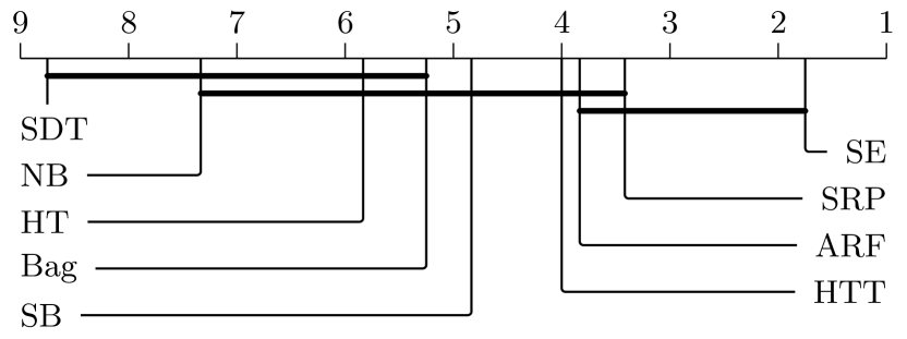
Figure 1: Critical Difference Diagram for the normalized area under the Pareto Front for different methods over multiple datasets. For all statistical tests $p=0.95$ was used. More to the right (lower rank) is better. Methods in connected cliques are statistically similar.

Table 1 shows the normalized area under the Pareto front. It can be seen that SE and SRP generally performs best followed by ARF. Our SE method ranks first on 7 datasets offering the best accuracy-memory trade-off followed by SRP which ranks first on 4 datasets. On the third place we find ARF which ranks first on the rbf_m dataset. SDT does not perform well. We hypothesize that this is due to the random initialization combined with the vanishing gradient problem. On the led_g dataset it did not finish the computation in under 2 hours and thus was removed for our evaluation. To give a statistical meaningful comparison we present the results in Table 1 as a CD diagram (Demšar 2006). In a CD diagram each method is ranked according to its performance and a Friedman-Test is used to determine if there is a statistical difference between the average rank of each method. If this is the case, then a pairwise Wilcoxon-Test between all methods checks whether there is a statistical difference between two classifiers. CD diagrams visualize this evaluation by plotting the average rank of each method on the x-axis and connect all classifiers whose performances are statistically similar via a horizontal bar. Figure 1 shows the corresponding CD diagram, where $p=0.95$ was used for all statistical tests. It can be seen that SE ranks first with an average rank between $1-2$ with some distance to SRP which – on average – ranks between $3-4$th place closely followed by ARF. Next, there is $\{SRP,ARF,HTT,SB,Bag,HT,NB\}$ which form a second clique and $\{Bag,HT,NB,SDT\}$ which forms the last clique. While all three methods $\{SE,SRP,ARF\}$ are in the same clique and hence offer similar performance, SE has some distance. It is only present in this clique meaning that it is statistically better than $\{HTT,SB,Bag,HT,NB,SDT\}$.

Qualitative Analysis

To gain a more complete picture we now inspect the iterative development of the test-then-train accuracy and the model size over the learning process for the best performing configuration of each algorithm without any memory constraints. Figures 2 and 3 plot the number of seen data points against the accuracy and memory requirement for the gas-sensor and led_a dataset. The gas-sensor dataset is interesting because it contains real-world data with a known time of drift whereas the led_a dataset contain artificial drift. Looking at the accuracy in Figure 2 (top row) we notice a rather chaotic behavior in the beginning, which can be attributed to the fact that in the first 10 months of measurements new classes appear for the first time. Once each class was presented at-least once to the algorithms, the accuracy approaches one, where SE has the highest accuracy, followed by SRP. After roughly $4,000$ datapoints we see a drop in the accuracy of ARF and NB which can be attributed to sudden changes in the distribution after roughly 20 month of measurements. Here, the number of measurements, as well as the class distribution heavily changes. We also observe that HTT seems to cope better with the dynamic changes in this dataset, compared to HT, which can be expected from the more greedy nature of the algorithm.

Figure 2: Accuracy and memory consumption over the number of items on the gas-sensor dataset. Best viewed in color.

Looking at the memory consumption in Figure 2 (bottom row) we notice an interesting behavior (note the logarithmic scale). We see that SE uses by far the fewest, strictly bounded resources whereas the other algorithm require at least a magnitude more memory. As expected, the memory consumption of HT and HTT monotonously rises over time as these algorithms never remove any internal node from the tree. Moreover, HTT must maintain the list of all possible splits at all times, thereby requiring more memory than HT. Likewise, the use of multiple HT(T)s as base learners of ARF, SRP, Bagging and SB is reflected in the plot. In addition, ARF and SRP both utilize the ADWIN drift detector (Bifet and Gavalda 2007) which uses a variable sized sliding window. The window size is computed by Hoeffding’s Bound which is ideally suited if no specific distribution can be assumed. On the downside, the window size convergences comparably slow. As a result, the algorithms store additional information for large windows to detect a possible drift further increasing the memory consumption. Naive Bayes (NB) is a strong competitor to SE, but also requires roughly a magnitude more memory. Last, we notice that the memory consumption of SDT increases over time due to a large sliding window in the hyperparameter settings. We conclude that our SE method offers the best predictive performance in the gas-sensor dataset while using the fewest resources making it an ideal algorithm for resource-constrained environments.

Figure 3: Accuracy and memory consumption over the number of items on the led_a dataset. Best viewed in color.

Figure 3 shows the test-then-train accuracy (top row) and average model size (bottom row) for the led_a dataset. While the accuracy is relatively stable in the beginning we can see a clear drop around the 250,000 item mark and a smaller drop later at around 500,000 items. NB and HT seem to suffer the most from this concept drift, but also the other algorithms lose some predictive power. Again, SDT does not seem to learn anything at-all. Looking at the memory consumption, we see a similar picture as before: HT(T) and ensembles of HT(T) learners steadily increase their memory consumption over time, requiring up to 100 MB. NB and SDT have the smallest memory consumption wheres SE ranks third in memory consumption in this setting. Again, we find that SE offers excellent performance while ranking among the most resource-friendly methods.

5 Conclusions

In this paper we introduced Shrub Ensembles (SE) as a tree ensemble which is able to process large amounts of data with limited resources in a fast-paced way, while adapting to new situations on the fly. We noticed, that incremental tree learner never remove any nodes from the tree slowly increasing the memory consumption over time. Gradient-based tree learning, on the other hand, requires the costly computation of gradients through backpropagation, making the overall algorithm slow. In contrast, Shrub Ensembles are ensembles of small- to medium sized trees which are aggressively pruned during optimization, such that sub-optimal shrubs are removed while new shrubs are regularly introduced. We theoretically showed that shrub ensembles will always add a new tree to the ensemble once a new, previously unknown concept is available (cf. Theorem 1). Further, we discussed the behavior of our algorithm on noisy data and the influence of its hyperparameters. Our Shrub Ensembles retain an excellent performance even when only little memory is available. In an extensive experimental study we showed that SE offers a better accuracy-memory trade-off in 7 of 12 cases, while having a statistically significant better performance than most other methods.

References

- Abdulsalam, Skillicorn, and Martin (2008) Abdulsalam, H.; Skillicorn, D. B.; and Martin, P. 2008. Classifying evolving data streams using dynamic streaming random forests. In International Conference on Database and Expert Systems Applications.
- Ahmetoğlu, İrsoy, and Alpaydın (2018) Ahmetoğlu, A.; İrsoy, O.; and Alpaydın, E. 2018. Convolutional Soft Decision Trees. In International Conference on Artificial Neural Networks, 134–141. Springer.
- Bergstra and Bengio (2012) Bergstra, J.; and Bengio, Y. 2012. Random search for hyper-parameter optimization. Journal of machine learning research, 13(2).
- Beygelzimer et al. (2015) Beygelzimer, A.; Hazan, E.; Kale, S.; and Luo, H. 2015. Online gradient boosting. NeurIPS, 2458–2466.
- Biau, Scornet, and Welbl (2019) Biau, G.; Scornet, E.; and Welbl, J. 2019. Neural Random Forests. Sankhya A.
- Bifet and Gavalda (2007) Bifet, A.; and Gavalda, R. 2007. Learning from time-changing data with adaptive windowing. In Proceedings of the 2007 SIAM international conference on data mining, 443–448. SIAM.
- Bifet and Gavalda (2009) Bifet, A.; and Gavalda, R. 2009. Adaptive learning from evolving data streams. In International Symposium on Intelligent Data Analysis, 249–260. Springer.
- Bifet et al. (2010) Bifet, A.; Holmes, G.; Kirkby, R.; and Pfahringer, B. 2010. MOA: Massive Online Analysis. J. Mach. Learn. Res., 11: 1601–1604.
- Bifet, Holmes, and Pfahringer (2010) Bifet, A.; Holmes, G.; and Pfahringer, B. 2010. Leveraging Bagging for Evolving Data Streams. In Machine Learning and Knowledge Discovery in Databases, 135–150. ISBN 978-3-642-15880-3.
- Chen, Lin, and Lu (2012) Chen, S.-t.; Lin, H.-t.; and Lu, C.-j. 2012. An Online Boosting Algorithm with Theoretical Justifications. ICML, 1007—-1014.
- Chen and Guestrin (2016) Chen, T.; and Guestrin, C. 2016. Xgboost: A scalable tree boosting system. In Proceedings of the 22nd acm sigkdd international conference on knowledge discovery and data mining, 785–794.
- Da Xu, He, and Li (2014) Da Xu, L.; He, W.; and Li, S. 2014. Internet of things in industries: A survey. IEEE Transactions on industrial informatics, 10(4): 2233–2243.
- Demšar (2006) Demšar, J. 2006. Statistical comparisons of classifiers over multiple data sets. The Journal of Machine Learning Research, 7: 1–30.
- Domingos and Hulten (2000) Domingos, P.; and Hulten, G. 2000. Mining high-speed data streams. In Proceeding of the Sixth ACM SIGKDD International Conference on Knowledge Discovery and Data Mining. ISBN 1581132336.
- Frosst and Hinton (2017) Frosst, N.; and Hinton, G. 2017. Distilling a neural network into a soft decision tree. arXiv.
- Geurts, Ernst, and Wehenkel (2006) Geurts, P.; Ernst, D.; and Wehenkel, L. 2006. Extremely randomized trees. Machine learning, 63(1): 3–42.
- Gomes et al. (2017a) Gomes, H. M.; Barddal, J. P.; Enembreck, F.; and Bifet, A. 2017a. A survey on ensemble learning for data stream classification.
- Gomes et al. (2017b) Gomes, H. M.; Bifet, A.; Read, J.; Barddal, J. P.; Enembreck, F.; Pfharinger, B.; Holmes, G.; and Abdessalem, T. 2017b. Adaptive random forests for evolving data stream classification. Machine Learning, 106(9): 1469–1495.
- Gomes, Read, and Bifet (2019) Gomes, H. M.; Read, J.; and Bifet, A. 2019. Streaming random patches for evolving data stream classification. In Proceedings - IEEE International Conference on Data Mining, ICDM. ISBN 9781728146034.
- Hochreiter (1998) Hochreiter, S. 1998. The vanishing gradient problem during learning recurrent neural nets and problem solutions. International Journal of Uncertainty, Fuzziness and Knowledge-Based Systems, 6(02): 107–116.
- Hoens, Chawla, and Polikar (2011) Hoens, T. R.; Chawla, N. V.; and Polikar, R. 2011. Heuristic updatable weighted random subspaces for non-stationary environments. In IEEE International Conference on Data Mining, 241–250.
- Holmes, Kirkby, and Pfahringer (2005) Holmes, G.; Kirkby, R.; and Pfahringer, B. 2005. Stress-testing hoeffding trees. In Lecture Notes in Computer Science. ISBN 3540292446.
- Hulten, Spencer, and Domingos (2001) Hulten, G.; Spencer, L.; and Domingos, P. 2001. Mining time-changing data streams. In Proceedings of the seventh ACM SIGKDD international conference on Knowledge discovery and data mining, 97–106.
- Irsoy and Alpaydın (2021) Irsoy, O.; and Alpaydın, E. 2021. Dropout regularization in hierarchical mixture of experts. Neurocomputing, 419: 148–156.
- Irsoy, Yildiz, and Alpaydin (2012) Irsoy, O.; Yildiz, O. T.; and Alpaydin, E. 2012. Soft decision trees. In International Conference on Pattern Recognition. ISBN 9784990644109.
- Ke et al. (2017) Ke, G.; Meng, Q.; Finley, T.; Wang, T.; Chen, W.; Ma, W.; Ye, Q.; and Liu, T.-Y. 2017. Lightgbm: A highly efficient gradient boosting decision tree. NeuIPS, 30: 3146–3154.
- Kolter and Maloof (2005) Kolter, J. Z.; and Maloof, M. A. 2005. Using additive expert ensembles to cope with concept drift. In Proceedings of the 22nd international conference on Machine learning, 449–456.
- Kontschieder et al. (2015) Kontschieder, P.; Fiterau, M.; Criminisi, A.; and Bulo, S. R. 2015. Deep neural decision forests. In Proceedings of the IEEE International Conference on Computer Vision. ISBN 9781467383912.
- Krawczyk et al. (2017) Krawczyk, B.; Minku, L. L.; Gama, J.; Stefanowski, J.; and Woźniak, M. 2017. Ensemble learning for data stream analysis: A survey. Information Fusion, 37: 132–156.
- Kubat (1989) Kubat, M. 1989. Floating approximation in time-varying knowledge bases. Pattern recognition letters, 10(4): 223–227.
- Kumar, Goyal, and Varma (2017) Kumar, A.; Goyal, S.; and Varma, M. 2017. Resource-efficient machine learning in 2 KB RAM for the Internet of Things. In 34th International Conference on Machine Learning, ICML 2017. ISBN 9781510855144.
- Kyrillidis et al. (2013) Kyrillidis, A.; Becker, S.; Cevher, V.; and Koch, C. 2013. Sparse projections onto the simplex. 30th International Conference on Machine Learning, ICML 2013, 28(PART 2): 894–902.
- Loh and Nowozin (2013) Loh, P.-L.; and Nowozin, S. 2013. Faster hoeffding racing: Bernstein races via jackknife estimates. In International Conference on Algorithmic Learning Theory, 203–217. Springer.
- Manapragada, Webb, and Salehi (2018) Manapragada, C.; Webb, G. I.; and Salehi, M. 2018. Extremely fast decision tree. In Proceedings of the ACM SIGKDD International Conference on Knowledge Discovery and Data Mining. ISBN 9781450355520.
- Maron and Moore (1993) Maron, O.; and Moore, A. W. 1993. Hoeffding races: Accelerating model selection search for classification and function approximation.
- Maron and Moore (1997) Maron, O.; and Moore, A. W. 1997. The racing algorithm: Model selection for lazy learners. Artificial Intelligence Review, 11(1): 193–225.
- Mirkhan, Amir Haeri, and Meybodi (2019) Mirkhan, M.; Amir Haeri, M.; and Meybodi, M. R. 2019. Analytical Split Value Calculation for Numerical Attributes in Hoeffding Trees with Misclassification-Based Impurity. Annals of Data Science.
- Oza (2005) Oza, N. C. 2005. Online bagging and boosting. In IEEE International Conference on Systems, Man and Cybernetics.
- Paszke et al. (2019) Paszke, A.; et al. 2019. PyTorch: An Imperative Style, High-Performance Deep Learning Library. In Advances in Neural Information Processing Systems 32, 8024–8035.
- Pawlak (1982) Pawlak, Z. 1982. Rough sets. International journal of computer & information sciences, 11(5): 341–356.
- Pelossof et al. (2009) Pelossof, R.; Jones, M.; Vovsha, I.; and Rudin, C. 2009. Online coordinate boosting. In 2009 IEEE 12th International Conference on Computer Vision Workshops, ICCV Workshops, 1354–1361. IEEE.
- Pfahringer, Holmes, and Kirkby (2007) Pfahringer, B.; Holmes, G.; and Kirkby, R. 2007. New Options for Hoeffding Trees. In AI 2007: Advances in Artificial Intelligence, 90–99. ISBN 978-3-540-76928-6.
- Pfahringer, Holmes, and Kirkby (2008) Pfahringer, B.; Holmes, G.; and Kirkby, R. 2008. Handling Numeric Attributes in Hoeffding Trees. In Advances in Knowledge Discovery and Data Mining, 296–307. ISBN 978-3-540-68125-0.
- Prokhorenkova et al. (2018) Prokhorenkova, L.; Gusev, G.; Vorobev, A.; Dorogush, A. V.; and Gulin, A. 2018. CatBoost: unbiased boosting with categorical features. In NeurIPS, volume 31.
- Reichler, Harris, and Savchenko (2004) Reichler, J. A.; Harris, H. D.; and Savchenko, M. A. 2004. Online parallel boosting. In AAAI, 366–371.
- Rutkowski et al. (2013) Rutkowski, L.; Pietruczuk, L.; Duda, P.; and Jaworski, M. 2013. Decision trees for mining data streams based on the mcdiarmid’s bound. IEEE Transactions on Knowledge and Data Engineering.
- Scholz and Klinkenberg (2005) Scholz, M.; and Klinkenberg, R. 2005. An ensemble classifier for drifting concepts. In Second International Workshop on Knowledge Discovery in Data Streams, volume 6, 53–64. Porto, Portugal.
- Seyedhosseini and Tasdizen (2015) Seyedhosseini, M.; and Tasdizen, T. 2015. Disjunctive normal random forests. Pattern Recognition.
- Shen et al. (2018) Shen, W.; Guo, Y.; Wang, Y.; Zhao, K.; Wang, B.; and Yuille, A. 2018. Deep Regression Forests for Age Estimation. In IEEE Computer Society Conference on Computer Vision and Pattern Recognition. ISBN 9781538664209.
- Street and Kim (2001) Street, W. N.; and Kim, Y. 2001. A streaming ensemble algorithm (SEA) for large-scale classification. In Proceedings of the seventh ACM SIGKDD international conference on Knowledge discovery and data mining, 377–382.
- Tanno et al. (2019) Tanno, R.; Arulkumaran, K.; Alexander, D. C.; Criminisi, A.; and Nori, A. 2019. Adaptive neural trees. In 36th International Conference on Machine Learning, ICML 2019. ISBN 9781510886988.
- Wang and Carreira-Perpinan (2013) Wang, W.; and Carreira-Perpinan, M. A. 2013. Projection onto the probability simplex: An efficient algorithm with a smple proof and an application.
- Widmer and Kubat (1996) Widmer, G.; and Kubat, M. 1996. Learning in the presence of concept drift and hidden contexts. Machine learning, 23(1): 69–101.
- Yildiz and Alpaydin (2014) Yildiz, O. T.; and Alpaydin, E. 2014. Regularizing soft decision trees. Lecture Notes in Electrical Engineering, 264 LNEE: 15–21.