IPPP/21/38, SI-HEP-2021-026, SFB-257-P3H-21-071

$SU(3)$ breaking effects in $B$ and $D$ meson lifetimes

Daniel King^(a), Alexander Lenz^(b) and Thomas Rauh^(c)
$(a)$ IPPP, Department of Physics, University of Durham,
DH1 3LE, United Kingdom
$(b)$ CPPS, Theoretische Physik 1, Department Physik, Universität Siegen, Walter-Flex-Straße 3, 57068 Siegen, Germany
$(c)$ Albert Einstein Center for Fundamental Physics,
Institute for Theoretical Physics, University of Bern,
Sidlerstrasse 5, CH-3012 Bern, Switzerland

Abstract

In the heavy quark expansion (HQE) of the total decay rates of $B_{s}$ and $D_{s}^{+}$ mesons non-perturbative matrix elements of four quark operators are arising as phase space enhanced contributions. We present the first determination of $m_{s}$ effects to the dimension six matrix elements of these four quark operators via a heavy quark effective theory (HQET) sum rule analysis. In addition we calculate for the first time eye contractions of the four quark operators as well as matrix elements of penguin operators. For the perturbative part we solve the 3-loop contribution to the sum rule and we evaluate condensate contributions. In this study we work in the strict HQET limit and our results can also be used to estimate the size of the matrix element of the Darwin operator via equations of motion.

1 Introduction

The theoretical predictions for $B$-meson lifetime ratios currently stand in close agreement with experimental results, see Table 1.

Lifetime Ratio	Experiment	Theory
$\frac{\tau(B^{+})}{\tau(B_{d})}$	$1.076\pm 0.004$ [1]	$1.078^{+0.021}_{-0.023}$[2]
$\frac{\tau(B_{s})}{\tau(B_{d})}$	$0.998\pm 0.005$ [1]	$1.0007\pm 0.0025$ [2]

Table 1: Experimental values (HFLAV [1]) of the lifetime ratio of $B$ mesons versus theoretical predictions based on the 2017 HQET sum rule prediction for the matrix elements of the four quark operators in the $\overline{MS}$ scheme [2].

The measurements of the $B_{s}$ lifetime have recently been updated by the LHCb collaboration [3, 4], the ATLAS collaboration [5] and by the CMS collaboration [6] and interestingly the value of ATLAS deviates from the other measurements [7]. In future we expect a further improvement of the experimental precision indicated in Table 1. On the theory side there has also been significant progress in the last years. According to the heavy quark expansion (HQE) [8, 9, 10, 11, 12, 13, 14, 15, 16] (see Ref. [17] for a recent review) the total decay rate of a hadron $H_{Q}$ containing a heavy quark $Q$ can be expanded in inverse powers of the heavy quark mass $m_{Q}$ and each term in the expansion is a product of a perturbative coefficient $\Gamma_{i}$ or $\tilde{\Gamma}_{i}$ and a non-perturbative matrix element of a $\Delta Q=0$ operator ${\cal O}_{D}$ or $\tilde{\cal O}_{D}$ of dimension $D$:

$$\Gamma = \Gamma_{3}\langle{\cal O}_{3}\rangle+\Gamma_{5}\frac{\langle{\cal O}_{5}\rangle}{m_{Q}^{2}}+\Gamma_{6}\frac{\langle{\cal O}_{6}\rangle}{m_{Q}^{3}}+...+16\pi^{2}\left[\tilde{\Gamma}_{6}\frac{\langle\tilde{{\cal O}}_{6}\rangle}{m_{Q}^{3}}+\tilde{\Gamma}_{7}\frac{\langle\tilde{{\cal O}}_{7}\rangle}{m_{Q}^{4}}+...\right]\,,$$ (1.1)

with $\langle{\cal O}_{D}\rangle=\langle H_{Q}|{\cal O}_{D}|H_{Q}\rangle/(2M_{H_{Q}})$. We denote with $\Gamma_{i}$ contributions related to two quark operators ${\cal O}_{i}$ and with $\tilde{\Gamma}_{i}$ contributions related to four quark operators $\tilde{\cal O}_{i}$. Each perturbative coefficient $\Gamma_{i}$ ($\tilde{\Gamma}_{i}$) can be further expanded in the strong coupling constant

$$\stackrel{{\scriptstyle\mathclap{\tiny\mbox{$(\sim)$}}}}{{\Gamma}}_{i}\,\,=\,\,{\stackrel{{\scriptstyle\mathclap{\tiny\mbox{$(\sim)$}}}}{{\Gamma}}_{i}}^{(0)}\!+\,\frac{\alpha_{s}}{4\pi}\,\,{\stackrel{{\scriptstyle\mathclap{\tiny\mbox{$(\sim)$}}}}{{\Gamma}}_{i}}^{(1)}\!+\left(\frac{\alpha_{s}}{4\pi}\right)^{2}\,{\stackrel{{\scriptstyle\mathclap{\tiny\mbox{$(\sim)$}}}}{{\Gamma}}_{i}}^{(2)}+\dots\,.$$ (1.2)

Traditionally the four quark contributions indicated by $\tilde{\Gamma}_{6}\langle\tilde{{\cal O}}_{6}\rangle$ are considered to give the dominant contributions to lifetimes ratios, because of the phase space enhancement factor $16\pi^{2}$, see e.g. Refs. [18, 19]. In these so-called spectator contributions, which are known to NLO-QCD accuracy [20, 21, 22, 23], the by far largest source of uncertainty resides in the non-perturbative hadronic matrix elements $\langle\tilde{{\cal O}}_{6}\rangle$. The most recent estimates for these parameters from lattice QCD [24] were carried out in 2001 and only made public in proceedings. In 2017 [2] a significant improvement to the precision of the dimension-6 matrix elements was achieved by means of a 3-loop HQET sum rule analysis. In that case, spectator mass effects in the sum rule were neglected. This is a sensible simplification for $B^{+}$ and $B_{d}$ mesons, where the spectator quark is an up or down quark. In the case of the $B_{s}$ meson however, $SU(3)_{F}$ breaking effects are not expected to be negligible. In this paper we present the first computation of the dimension-6 matrix elements of $\Delta Q=0$ four quark operators with a non-zero strange quark mass, following the method established in Ref. [25], where $m_{s}$ effects to the HQET sum rules for $B_{s}$ mixing were calculated. These efforts lead to results with a competitive precision for $B$ mixing observables, see Ref. [26], as modern lattice determinations [27, 28, 29] and to strong bounds on BSM models that try to explain the flavour anomalies, see e.g. Refs. [26, 30]. In addition we determine for the first time eye contractions of the $\Delta Q=0$ four quark operators as well as matrix elements of penguin operators.
Very recently the Darwin term $\Gamma_{6}\langle{\cal O}_{6}\rangle$ was calculated for the first time for non-leptonic decays and found to be very large [31, 32, 33]. For the lifetime ratio $\tau(B^{+})/\tau(B_{d})$ this contribution will cancel due to isospin symmetry. However, for a precise calculation of the ratio $\tau(B_{s})/\tau(B_{d})$ the $SU(3)_{F}$ breaking contribution of the form $\Gamma_{6}(\langle{\cal O}_{6}\rangle_{B_{d}}-\langle{\cal O}_{6}\rangle_{B_{s}})$ has to be determined. The matrix element $\langle{\cal O}_{6}\rangle_{B_{d}}$ is known quite well from fits of the inclusive semileptonic $B$ meson decays, see e.g. Refs. [34, 35], unfortunately a corresponding analysis has not been performed for the $B_{s}$ meson, thus $\langle{\cal O}_{6}\rangle_{B_{s}}$ is largely unknown. However, the Darwin operator can be related to four quark operators via equations of motion (see e.g. [32, 36]) and thus our results can also be used to estimate the size of the matrix element of the Darwin operator for the $B_{s}$ meson.
In the following sections, we will restrict our discussion to the calculation of the hadronic matrix elements themselves and reserve a full analysis of the $B$ lifetimes for a subsequent paper in which the results presented here will be used alongside other recent developments in the HQE [31, 32, 33].
Since we work here in the strict HQET limit our results can also be applied to the charm sector, where sizeable lifetime differences have been found experimentally [37, 38]:

$$\frac{\tau(D^{+})}{\tau(D_{0})}=2.54\pm 0.02\,,\hskip 28.45274pt\frac{\tau(D_{s}^{+})}{\tau(D_{0})}=1.20\pm 0.01\,.$$ (1.3)

As the expansion parameter $\alpha_{s}(m_{c})$ and $\Lambda/m_{c}$ where $\Lambda$ is a hadronic scale are quite sizeable, a study of charm lifetimes can shed light on the convergence radius of the HQE [36].
Our results can of course also be used for an analysis of spectator effects in inclusive semi-leptonic $B$ and $D$ meson decays, where the same matrix elements will appear, see e.g. Ref. [36].
The rest of this paper is arranged as follows: Section 2 consists of the sum rule setup and a collection of the analytic results. We introduce the operator basis and the parameterisation of the matrix elements in Section 2.1, while Section 2.2 is devoted to the presentation of the sum rule itself. The perturbative part of the sum rule is discussed in Section 2.3 including a brief overview of the determination of $m_{s}$ corrections as well as the introduction of the eye-contractions. Condensate contributions will be revisited in Section 2.4 and in Section 2.5 we present analytic results. In Section 3 we summarise the findings of our numerical analysis, and in Section 4 we conclude.

2 Setup and calculation

2.1 Operator Basis

We carry out the sum rule in the exact HQET limit in order to avoid mixing between operators of different mass dimensions. The basis we use coincides with that of Ref. [21], except for the naming of the colour-octett operators. In the HQET limit (denoted by the tilde) we get

$$\tilde{Q}_{1}^{q} = \bar{h}\gamma_{\mu}(1-\gamma^{5})q\cdot\bar{q}\gamma^{\mu}(1-\gamma^{5})h,\hskip 28.45274pt\tilde{T}_{1}^{q}=\bar{h}\gamma_{\mu}(1-\gamma^{5})T^{A}q\cdot\bar{q}\gamma^{\mu}(1-\gamma^{5})T^{A}h,$$

$$\tilde{Q}_{2}^{q} = \bar{h}(1-\gamma^{5})q\cdot\bar{q}(1+\gamma^{5})h,\hskip 52.63777pt\tilde{T}_{2}^{q}=\bar{h}(1-\gamma^{5})T^{A}q\cdot\bar{q}(1+\gamma^{5})T^{A}h,$$ (2.1)

where $h$ denotes the HQET field describing the heavy quark $Q$ with mass $m_{Q}$, the light quark fields are denoted by $q$. In addition we use the same evanescent operators as in Ref. [2] (choosing $a_{1}=a_{2}=-8$). A full description of SU(3) flavour-breaking contributions at NLO in QCD also requires us to consider the QCD penguin operators

$$\tilde{Q}_{P}^{q}=\bar{h}\gamma_{\mu}T^{A}h\cdot\bar{q}\gamma^{\mu}T^{A}q\,.$$ (2.2)

Note, that differing from the definition in Ref. [21] we need the flavour specific contribution of the penguins, thus we are not summing over the light quark flavour $q$. Inspired by Refs. [39, 21] we parametrize the matrix elements of the above operators as,

$$\braket{{\mathbf{B}}_{q}}{\tilde{Q}_{i}^{q}(\mu)}{{\mathbf{B}}_{q}} =A_{\tilde{Q}_{i}}F_{q}^{2}(\mu)\tilde{B}_{i}^{q}(\mu)\, \braket{{\mathbf{B}}_{q}}{\tilde{Q}_{i}^{q^{\prime}}(\mu)}{{\mathbf{B}}_{q}} =A_{\tilde{Q}_{i}}F_{q}^{2}(\mu)\tilde{\delta}_{i}^{q^{\prime}q}(\mu)\,,$$

$$\braket{{\mathbf{B}}_{q}}{\tilde{T}_{i}^{q}(\mu)}{{\mathbf{B}}_{q}} =A_{\tilde{T}_{i}}F_{q}^{2}(\mu)\tilde{\epsilon}_{i}^{q}(\mu) \braket{{\mathbf{B}}_{q}}{\tilde{T}_{i}^{q^{\prime}}(\mu)}{{\mathbf{B}}_{q}} =A_{\tilde{T}_{i}}F_{q}^{2}(\mu)\tilde{\delta}_{i+2}^{q^{\prime}q}(\mu)\,,$$

$$\braket{{\mathbf{B}}_{q}}{\tilde{Q}_{P}^{q}(\mu)}{{\mathbf{B}}_{q}} =A_{\tilde{Q}_{P}}F_{q}^{2}(\mu)\tilde{B}_{P}^{q}(\mu) \braket{{\mathbf{B}}_{q}}{\tilde{Q}_{P}^{q^{\prime}}(\mu)}{{\mathbf{B}}_{q}} =A_{\tilde{Q}_{P}}F_{q}^{2}(\mu)\tilde{\delta}_{P}^{q^{\prime}q}(\mu)\,,$$ (2.3)

for which the colour factors correspond to,

$$A_{\tilde{Q}_{i}}=A_{\tilde{T}_{i}}=1\hskip 28.45274ptA_{\tilde{Q}_{P}}=-\frac{C_{F}}{2N_{c}}\,,$$ (2.4)

with the HQET decay constant $F_{q}$, the bag parameters $\tilde{B}_{i}^{q}$, $\tilde{B}_{P}^{q}$ and $\tilde{\epsilon}_{i}^{q}$ and the non-valence contribution $\tilde{\delta}_{i}^{q^{\prime}q}$, for $q\neq q^{\prime}$. Note that differing from Refs. [21] and [39] we have included in $\tilde{B}_{i}^{q}$, $\tilde{B}_{P}^{q}$ and $\tilde{\epsilon}_{i}^{q}$ also the non-valence contributions with $q=q^{\prime}$. As usual $\mu$ denotes the renormalisation scale dependence. In addition the heavy $|{\mathbf{B}}_{q}\rangle$ meson states (consisting of a heavy anti-quark $\overline{Q}$ and a light quark ${q}$ ) are considered in the strict HQET limit and thus our expressions hold both for $B$ and $D$ mesons.

2.2 The Sum Rule

The HQET Borel sum rule for the decay constant $F_{q}$, as derived in Refs. [40, 41, 42, 43], is well studied. The starting point for its derivation is the 2-point correlator,

$$\Pi(\omega)=\int\;d^{d}xe^{ip\cdot x}\Braket{0}{\text{T}\left\{\tilde{j}_{q}(0)\tilde{j}_{q}^{\dagger}(x)\right\}}{0}$$ (2.5)

for a heavy meson with the momentum $p_{M}=m_{Q}v+p$, where $v$ is the four-velocity of the meson and $p$ the residual momentum. The residual energy is denoted by $\omega=p\cdot v$. The interpolating heavy meson current used in Eq.(2.5) is defined as,

$$\tilde{j}_{q}=\bar{q}\gamma^{5}h.$$ (2.6)

The sum rule for $F_{q}$ then takes the form of,

$$F^{2}_{q}(\mu)=\int\limits_{0}^{\omega_{c}}d\omega\;e^{\frac{\overline{\Lambda}_{q}-\omega}{t}}\rho_{\Pi}(\omega)$$ (2.7)

for which $\rho_{\Pi}(\omega)$ is defined as the discontinuity of Eq.(2.5), $\overline{\Lambda}_{q}$ is the meson mass-difference, the Borel parameter $t$ determines the degree to which continuum states of the hadronic spectral function are exponentially suppressed, and where we have introduced a cutoff of $\omega_{c}$.

In order to build a sum rule for the bag parameters however, the central object of the calculation is the 3-point correlator,

$$K_{\tilde{\mathcal{O}}^{q^{\prime}}}^{q}(\omega_{1},\omega_{2})=\int d^{d}x_{1}d^{d}x_{2}e^{i(p_{1}\cdot x_{1}-p_{2}\cdot x_{2})}\braket{0}{\text{T}\left\{\tilde{j}_{q}(x_{2})\tilde{\mathcal{O}}^{q^{\prime}}(0)\tilde{j}_{q}^{\dagger}(x_{1})\right\}}{0},$$ (2.8)

where $p_{i}$ corresponds to the residual momentum of the incoming and outgoing states respectively, each with velocity $v$, and residual energy $\omega_{1,2}=p_{1,2}\cdot v$, and in addition to the heavy quark currents there is now also the insertion of a four quark operator.

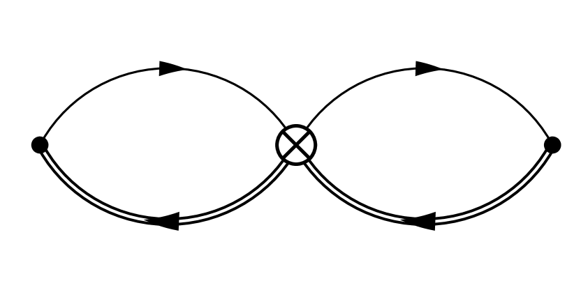
(a) LO Factorisable

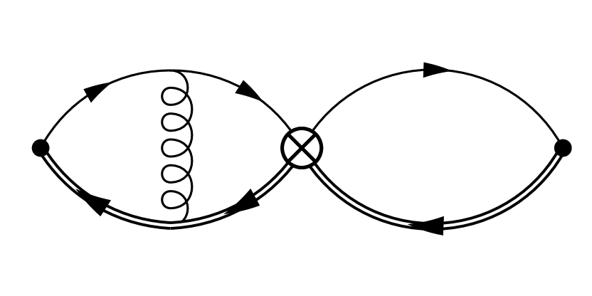
(b) NLO Factorisable

(c) NLO Nonfactorisable

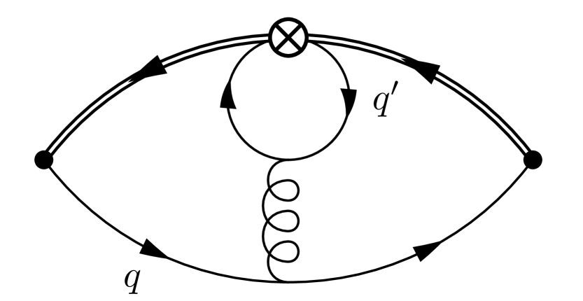
(d) NLO Non-Valence

Figure 1: Some of the diagrams contributing to the correletor in Eq.(2.8). Non-valence type diagrams like that shown in (d) only appear at NLO.

As in Refs. [2, 25] we categorise the possible field contractions of Eq.(2.8) into factorisable and non-factorisable contributions. Examples of the corresponding Feynman diagrams are found in Fig.1. This separation of contributions allows us to formulate a sum rule for the deviation of the bag parameter $\Delta B$ from its vacuum saturation approximation (VSA) value.

$$\tilde{B}_{i}^{q}(\mu) = 1+\Delta B^{q}_{\tilde{Q}_{i}^{q}}(\mu)\,,$$ (2.9)

$$\tilde{\epsilon}_{i}^{q}(\mu) = 0+\Delta B^{q}_{\tilde{T_{i}^{q}}}(\mu)\,,$$ (2.10)

$$\tilde{B}_{P}^{q}(\mu) = 1+\Delta B^{q}_{\tilde{Q}_{P}^{q}}(\mu)\,.$$ (2.11)

We find the following finite energy Borel sum rules,

$$\Delta B^{q}_{\tilde{\mathcal{O}}^{q}}(\mu)=\frac{1}{A_{\mathcal{O}}F_{q}^{4}(\mu)}\int\limits_{0}^{\omega_{c}}d\omega_{1}d\omega_{2}e^{\frac{\overline{\Lambda}_{q}-\omega_{1}}{t}+\frac{\overline{\Lambda}_{q}-\omega_{2}}{t}}\Delta\rho_{\tilde{\mathcal{O}}^{q}}^{q}(\omega_{1},\omega_{2})$$ (2.12)

in which the term $\Delta\rho_{\tilde{\mathcal{O}}^{q}}^{q}(\omega_{1},\omega_{2})$ corresponds to the non-factorisable part of the double discontinuity of Eq.(2.8). Looking at the whole double discontinuity of the 3-point correlator it is useful to separate out the various contributions further as,

$$\begin{split}\rho_{\tilde{\mathcal{O}}^{q}}^{q}(\omega_{1},\omega_{2})&=\delta_{\tilde{\mathcal{O}}\tilde{Q}}\rho_{\Pi}(\omega_{1})\rho_{\Pi}(\omega_{2})+\Delta\rho_{\tilde{\mathcal{O}}^{q}}^{q}(\omega_{1},\omega_{2})\\ &=\delta_{\tilde{\mathcal{O}}\tilde{Q}}\rho_{\Pi}(\omega_{1})\rho_{\Pi}(\omega_{2})+\Delta_{\text{tree}}\rho_{\tilde{\mathcal{O}}^{q}}^{q}(\omega_{1},\omega_{2})+\Delta_{\text{peng}}\rho_{\tilde{\mathcal{O}}^{q}}^{q}(\omega_{1},\omega_{2})\;,\end{split}$$ (2.13)

for which $\delta_{\tilde{\mathcal{O}}\tilde{Q}}$ is equal to 1 for the colour singlet and penguin operators and 0 for the colour octet operators. In Eq.(2.13), the first term corresponds to factorisable contributions, whilst $\Delta_{\text{tree}}\rho$ corresponds to the first set of non-factorisbale contractions (see Fig.1(c)). The term denoted by $\Delta_{\text{peng}}\rho$, stems from ‘eye-contraction’ diagrams like that of the example illustrated in Fig.1(d) and was not considered in [2] as these diagrams only become necessary when taking into account SU(3) flavour breaking effects. Note also, that these contributions first appear at NLO in QCD. The presence of the non-valence terms also forces us to expand our basis of operators to include the penguin operator defined in Eq.(2.2), which arises in renormalisation and thus mixes with the original basis under renormalisation group (RG) running. Details of the correlator renormalisation and the resulting structure of the renormalisation group equations (RGE) are presented in Appendix A. For the matrix elements of operators with a different light-quark flavour to that of the external meson state, only these ‘eye-contraction’ diagrams contribute and so the sum-rule has the form,

$$\delta^{q^{\prime}q}_{\tilde{\mathcal{O}}^{q^{\prime}}}(\mu)=\frac{1}{A_{\mathcal{O}}F_{q}^{4}(\mu)}\int\limits_{0}^{\omega_{c}}{d\omega_{1}d\omega_{2}e^{\frac{\overline{\Lambda}_{q}-\omega_{1}}{t}+\frac{\overline{\Lambda}_{q}-\omega_{2}}{t}}\Delta_{\text{peng}}\rho_{\tilde{\mathcal{O}}^{q^{\prime}}}^{q}(\omega_{1},\omega_{2})}$$ (2.14)

We further split the non-factorisables part into perturbative and condensate contributions

$$\Delta_{\text{tree/peng}}\rho_{\tilde{\mathcal{O}}^{q^{\prime}}}^{q}(\omega_{1},\omega_{2})=\Delta_{\text{tree/peng}}^{\text{pert}}\rho_{\tilde{\mathcal{O}}^{q^{\prime}}}^{q}(\omega_{1},\omega_{2})+\Delta_{\text{tree/peng}}^{\text{cond}}\rho_{\tilde{\mathcal{O}}^{q^{\prime}}}^{q}(\omega_{1},\omega_{2})\,,$$ (2.15)

where the tree contribution vanishes if $q\neq q^{\prime}$. Those will be discussed in greater depth in Section 2.3 and 2.4 and we show the results of our calculations in Section 2.5.

2.3 Perturbative contributions

As already mentioned, the eye-contraction diagrams represent a new contribution, not previously calculated, to our sum rule analysis of the $B_{s}$ lifetime matrix elements. The procedure for computing them however, is unchanged from that of the standard tree-contraction terms, which was performed and described in detail in Ref. [2, 25]. So here we will only briefly summarise our approach.
The three-point correlators were calculated using two separate implementations. In one, the amplitudes of the 3-loop processes were generated manually and the Dirac algebra was computed using Tracer [44], treating $\gamma^{5}$ in accordance with the Larin scheme [45]. Alternatively, the amplitudes were generated using QGRAF [46] and the Dirac algebra computed using a private implementation in the ‘NDR’ scheme. We found full agreement between both computations. An ‘Integration by Parts’ [47] reduction of the amplitudes was carried out using FIRE5 [48]. The resulting master integrals are already known [49] to all orders in $\epsilon$ and we expanded these to the required order using the HypExp package [50]. These master integrals describe the massless spectator quark scenario. In order to compute the $m_{s}$ corrections, an ‘expansion by regions’ approach was taken [51, 52] and leads to a Taylor expansion in $m_{s}/\omega$, allowing us to ‘recycle’ the master integrals of the massless case.
In this work, it became apparent that when considering $m_{s}$ corrections to the eye-contractions, these contributions could only be treated consistently within the traditional sum rule approach and not with the weight function method used in Refs. [2, 25]. Therefore in this work we explicitly evaluate the integrals in Eq.(2.12) and Eq.(2.14) in the traditional sum rule framework. However, when applicable we compare the results of both methods and show that we find them to be consistent. This will be discussed further in Sections 2.5 and 3. There are two major consequences resulting from shifting towards a traditional sum rule approach. The first is that when also using the HQET sum rule result for the decay constant (as shown in Eq.(2.7)), the dependency of the bag parameter on $\overline{\Lambda}_{q}$ drops out. The second is that there is now an explicit dependence of the bag parameter on both the cut-off $\omega_{c}$ and the Borel parameter $t$. In our implementation, these parameters were set by fixing the HQET sum rules for $F_{q}$ and $\overline{\Lambda}_{q}$ to values found in the literature. Details of this procedure can be found in Appendix D.

2.4 Condensate contributions

We also carried out an independent analysis of the condensate contributions, that have previously been determined for the massless case in Refs. [53, 54] for the $Q_{i}$ and $T_{i}$ operators, but not for $Q_{P}$. Whenever appropriate we compare our results with the literature in Section 2.5.
We use the standard approach of the background field method [55, 56, 57]. Since, in calculating the deviation of the bag parameters from their VSA values, we are only concerned with non-factorisable contributions, the only diagrams that need to be considered are those found in Fig. 2 along with their symmetric counterparts. These represent the only condensate corrections up to dimension-6 and leading order in $\alpha_{s}$, assuming that the quark condensate factorises and thus leads to no correction to the non-factorisable contribution.
With regards to the non-valence terms, there is no dimension three quark condensate contribution at the leading order in $\alpha_{s}$ from the diagrams in Fig. 3. The left diagram vanishes because the quark condensate flips the chirality and the Dirac structure $\Gamma_{1}\langle\bar{q}^{\prime}q^{\prime}\rangle\Gamma_{2}$ vanishes for all the combinations of currents $\Gamma_{1,2}$ appearing in the considered operators. The $\langle\bar{q}^{\prime}q^{\prime}\rangle$ condensate is therefore suppressed by an additional $\alpha_{s}m_{q^{\prime}}/\overline{\Lambda}$. The right diagram is scaleless. The $\langle\bar{q}q\rangle$ condensate is therefore suppressed by at least an extra $\alpha_{s}$. There is also no dimension four gluon condensate $\langle\alpha_{s}G^{2}\rangle$ contribution at leading order in $\alpha_{s}$ because the penguin loop is scaleless without an extra gluon. Similar arguments lead us to conclude that the dimension five quark gluon condensate $\langle\bar{q}^{(^{\prime})}\sigma_{\mu\nu}G^{\mu\nu}q^{(^{\prime})}\rangle$ and the dimension six quark condensate $\langle\bar{q}^{\prime}q^{\prime}\bar{q}q\rangle$ do not contribute at leading order in $\alpha_{s}$. Therefore, condensate contributions to the eye-contractions are suppressed with respect to the perturbative contribution at first order in the strong coupling and are not taken into account.

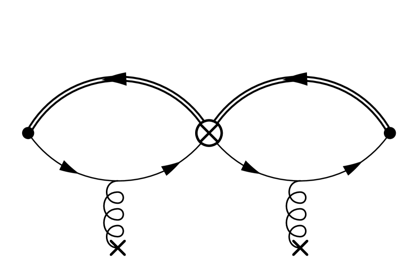
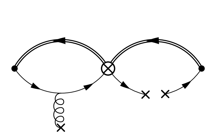
Figure 2: Condensate corrections corresponding to $\braket{\frac{\alpha_{s}}{4\pi}GG}$ and $\braket{g_{s}\overline{q}\sigma_{\mu\nu}G^{\mu\nu}q}$ respectively.

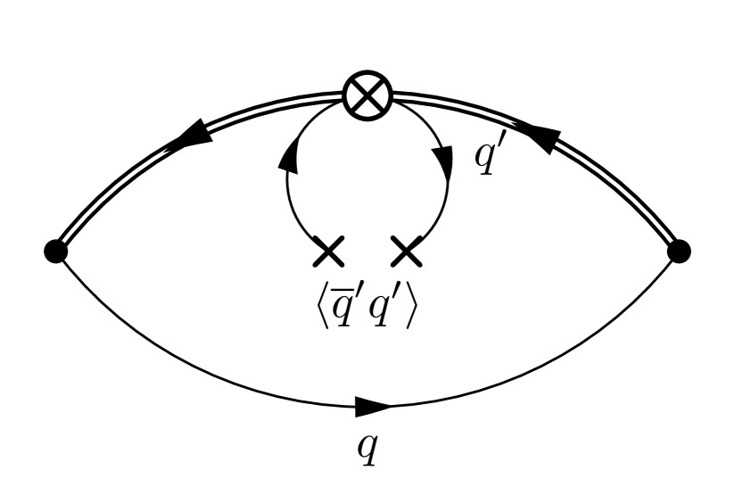
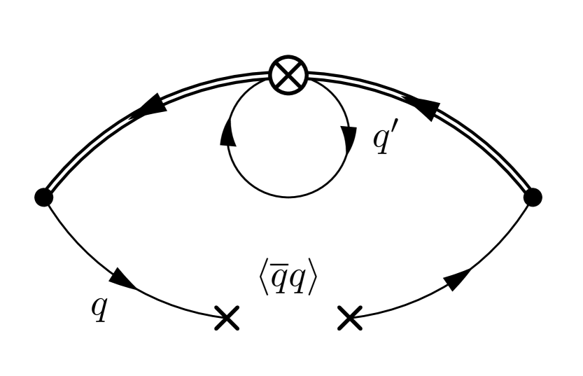
Figure 3: Quark condensate contributions to the eye contractions at leading order in $\alpha_{s}$.

2.5 Analytic results

In this section we present the analytic expressions of our calculation. Beginning with the perturbative contribution, the double discontinuities defined in Eq.(2.13) can be expressed in terms of their $m_{s}$ (generally denoted as $m_{q}$ below) expansion as,

$$\Delta_{\text{tree}}^{\text{pert}}\rho_{\tilde{\mathcal{O}}^{q}}^{q}(\omega_{1},\omega_{2})\equiv\, \frac{N_{c}C_{F}}{4}\frac{\omega_{1}^{2}\omega_{2}^{2}}{\pi^{4}}\frac{\alpha_{s}}{4\pi}\Bigg{[}r_{\tilde{\mathcal{O}}}^{(0)}(x,L_{\omega})+\left(\frac{m_{q}}{\omega_{1}}+\frac{m_{q}}{\omega_{2}}\right)r_{\tilde{\mathcal{O}}}^{(1)}(x,L_{\omega})$$

$$+\left(\frac{m_{q}^{2}}{\omega_{1}^{2}}+\frac{m_{q}^{2}}{\omega_{2}^{2}}\right)r_{\tilde{\mathcal{O}}}^{(2)}(x,L_{\omega})+\dots\Bigg{]}\,\theta(\omega_{1}-m_{q})\theta(\omega_{2}-m_{q}),$$ (2.16)

for $x=\omega_{2}/\omega_{1}$ and $L_{\omega}=\ln(\mu^{2}/(4\omega_{1}\omega_{2}))$.
The non-factorisable tree contributions for the colour singlet operators at order $\alpha_{s}$ have a vanishing color factor, yielding $r_{\tilde{Q}_{i}}^{(j)}=0$. In the massless limit we find [2]

$$r_{\tilde{T}_{1}}^{(0)} = -8+\frac{a_{1}}{8}+\frac{2\pi^{2}}{3}-\frac{3}{2}L_{\omega}-\frac{1}{4}\phi(x)\,,$$

$$r_{\tilde{T}_{2}}^{(0)} = -\frac{29}{4}+\frac{a_{2}}{8}+\frac{2\pi^{2}}{3}-\frac{3}{2}L_{\omega}-\frac{1}{4}\phi(x)\,,$$ (2.17)

and

$$r_{\tilde{Q}_{P}}^{(0)}=\frac{1}{8N_{c}}\left[-30+\frac{8\pi^{2}}{3}-6L_{\omega}-\phi(x)\right]\,,$$ (2.18)

for the penguin operator, where

$$\phi(x)=\begin{cases}x^{2}-8x+6\ln(x),\hskip 28.45274ptx\leq 1,\\ \frac{1}{x^{2}}-\frac{8}{x}-6\ln(x),\hskip 34.14322ptx>1.\end{cases}$$ (2.19)

The linear terms in the strange quark mass read

$$r_{\tilde{T}_{1}}^{(1)} = \frac{a_{1}}{8}+\frac{2\pi^{2}}{3}-\frac{3}{2}L_{\omega}-\begin{cases}\frac{2(36+9x+x^{2})}{9(1+x)}+\frac{9+9x-2x^{2}}{6(1+x)}\ln(x),&x\leq 1,\\ \frac{2(1+9x+36x^{2})}{9x(1+x)}+\frac{2-9x-9x^{2}}{6x(1+x)}\ln(x),&x>1,\end{cases}$$

$$r_{\tilde{T}_{2}}^{(1)} = \frac{a_{2}}{8}+\frac{2\pi^{2}}{3}-\frac{3}{2}L_{\omega}+\begin{cases}-\frac{29+11x-2x^{2}}{4(1+x)}-\frac{3}{2}\ln(x),&x\leq 1,\\ \frac{2-11x-29x^{2}}{4x(1+x)}+\frac{3}{2}\ln(x),&x>1,\end{cases}$$ (2.20)

$$r_{\tilde{Q}_{P}}^{(1)} = \frac{1}{36N_{c}}\Bigg{[}-12\pi^{2}+27L_{\omega}+\begin{cases}\frac{135+81x-22x^{2}}{1+x}+\frac{3(9+9x+2x^{2})}{1+x}\ln(x),&x\leq 1,\\ -\frac{22-81x-135x^{2}}{x(1+x)}-\frac{3(2+9x+9x^{2})}{x(1+x)}\ln(x),&x>1,\end{cases}\Bigg{]}$$

and for the corrections quadratic in $m_{s}$ we find

$$r_{\tilde{T}_{1}}^{(2)} = \frac{1}{1+x^{2}}\left[-\frac{(1-x)^{2}a_{1}}{16}+\frac{3(1-x)^{2}}{4}L_{\omega}-\frac{x}{4}\psi(x)\left(1+\frac{3(1+x)}{1-x}\ln(x)\right)\right.$$

$$\left.+\begin{cases}\frac{\pi^{2}(1+8x-5x^{2})}{12}+\frac{24-48x+16x^{2}+x^{3}}{6}+\frac{1+x^{2}}{2}\ln(x)&\\ +\frac{1-x^{2}}{2}\ln^{2}(x)+\frac{5(1-x^{2})}{2}\text{Li}_{2}\left(1-\frac{1}{x}\right),&x\leq 1,\\ \\ \frac{\pi^{2}(-5+8x+x^{2})}{12}+\frac{1+16x-48x^{2}+24x^{3}}{6x}-\frac{1+x^{2}}{2}\ln(x)&\\ -\frac{1-x^{2}}{2}\ln^{2}(x)-\frac{5(1-x^{2})}{2}\text{Li}_{2}(1-x),&x>1,\end{cases}\right],$$

$$r_{\tilde{T}_{2}}^{(2)} = \frac{1}{1+x^{2}}\left[-\frac{a_{2}(1-x)^{2}}{16}-\frac{\pi^{2}(1-4x+x^{2})}{6}+\frac{3(1-x)^{2}}{4}L_{\omega}\right.$$ (2.21)

$$+\frac{29-62x+29x^{2}}{8}-\frac{x}{2}\psi(x)\left(1+\frac{1+x}{1-x}\ln(x)\right)$$

$$\left.+\begin{cases}\frac{(1-x)^{2}}{4}\ln(x)+(1-x^{2})\text{Li}_{2}\left(1-\frac{1}{x}\right),&x\leq 1,\\ -\frac{(1-x)^{2}}{4}\ln(x)-(1-x^{2})\text{Li}_{2}\left(1-x\right),&x>1,\end{cases}\right],$$

$$r_{\tilde{Q}_{P}}^{(2)} = \frac{1}{24N_{c}(1+x^{2})}\left[9(1-x)^{2}L_{\omega}-9x\psi(x)\left(1+\frac{1+x}{3(1-x)}\ln(x)\right)\right.$$

$$\left.+\begin{cases}45-102x+61x^{2}-2x^{3}-(5-8x-x^{2})\pi^{2}-12x\ln(x)&\\ -6(1-x^{2})\ln^{2}(x)-6(1-x^{2})\text{Li}_{2}\left(1-\frac{1}{x}\right),&x\leq 1,\\ \\ -\frac{2-61x+102x-45x^{3}}{x}+(1+8x-5x^{2})\pi^{2}+12x\ln(x)&\\ +6(1-x^{2})\ln^{2}(x)+6(1-x^{2})\text{Li}_{2}\left(1-x\right),&x>1,\end{cases}\right]$$

with

$$\psi(x)=\begin{cases}\frac{(1-x)^{2}}{x}\left[2\ln(1-x)-\ln(x)\right],\hskip 28.45274ptx\leq 1,\\ \frac{(1-x)^{2}}{x}\left[2\ln(x-1)-\ln(x)\right],\hskip 28.45274ptx>1.\end{cases}$$ (2.22)

The perturbative contribution to the double discontinuities of the eye-contractions, defined in Eq.(2.13), can be expressed in terms of their $m_{s}$ (generally denoted as $m_{q}$ and $m_{q^{\prime}}$ below) expansion as

$$\Delta_{\text{peng}}^{\text{pert}}\rho_{\tilde{\mathcal{O}}^{q^{\prime}}}^{q}(\omega_{1},\omega_{2})\equiv\, \frac{N_{c}C_{F}}{4}\frac{\omega_{1}^{2}\omega_{2}^{2}}{\pi^{4}}\frac{\alpha_{s}}{4\pi}\Bigg{[}s_{\tilde{\mathcal{O}}}^{(0)}(x,L_{\omega})+\left(\frac{m_{q}}{\omega_{1}}+\frac{m_{q}}{\omega_{2}}\right)s_{\tilde{\mathcal{O}}}^{(1)}(x,L_{\omega})$$

$$+\left(\frac{1}{\omega_{1}^{2}}+\frac{1}{\omega_{2}^{2}}\right)\left[m_{q}^{2}s_{\tilde{\mathcal{O}}}^{(2)}(x,L_{\omega})+m_{q^{\prime}}^{2}t_{\tilde{\mathcal{O}}}^{(2)}(x,L_{\omega})\right]+\dots\Bigg{]}$$

$$\times\theta(\omega_{1}-m_{q})\theta(\omega_{2}-m_{q}).$$ (2.23)

For the non-valence expression Eq.(2.23), $s_{\tilde{\mathcal{O}}}^{(i)}$ corresponds to $m_{s}$ corrections of order $i$ stemming from a non-zero $q$ quark mass (see Fig.1), whereas $m_{s}$ corrections attributed to the $q^{\prime}$ quark are contained within the $t_{\tilde{\mathcal{O}}}^{(2)}$ term. It is also worth noting that there is no $t_{\tilde{\mathcal{O}}}^{(1)}$ in Eq.(2.23) since the double discontinuity evaluates to zero.

At the considered order the eye contributions for the color singlet and octet operators differ only by their color factors

$$s_{\tilde{T}_{i}}^{(j)}=\frac{-1}{2N_{c}}\,s_{\tilde{Q}_{i}}^{(j)},\hskip 28.45274ptt_{\tilde{T}_{i}}^{(2)}=\frac{-1}{2N_{c}}\,t_{\tilde{Q}_{i}}^{(2)}.$$ (2.24)

Our results for the singlet and penguin operators are in the massless case

$$s_{\tilde{Q}_{1}}^{(0)} = \frac{20}{9}+\frac{2}{3}L_{\omega}+\frac{1}{9}\phi(x),$$

$$s_{\tilde{Q}_{2}}^{(0)} = -\frac{13}{9}-\frac{1}{3}L_{\omega}-\frac{1}{18}\phi(x),$$

$$s_{\tilde{Q}_{P}}^{(0)} = \frac{13}{9}+\frac{1}{3}L_{\omega}+\frac{1}{18}\phi(x).$$ (2.25)

The corrections proportional to the strange quark mass read

$$s_{\tilde{Q}_{1}}^{(1)} = \frac{2}{3}L_{\omega}+\begin{cases}\frac{2(10+x-x^{2})}{9(1+x)}+\frac{2}{3}\ln(x),&x\leq 1,\\ -\frac{2(1-x-10x^{2})}{9x(1+x)}-\frac{2}{3}\ln(x),&x>1,\end{cases},$$

$$s_{\tilde{Q}_{2}}^{(1)} = -\frac{1}{3}L_{\omega}+\begin{cases}-\frac{13+4x-x^{2}}{9(1+x)}-\frac{1}{3}\ln(x),&x\leq 1,\\ \frac{1-4x-13x^{2}}{9x(1+x)}+\frac{1}{3}\ln(x),&x>1,\end{cases},$$

$$s_{\tilde{Q}_{P}}^{(1)} = -\frac{1}{3}L_{\omega}+\begin{cases}-\frac{13+4x-x^{2}}{9(1+x)}-\frac{1}{3}\ln(x),&x\leq 1,\\ \frac{1-4x-13x^{2}}{9x(1+x)}+\frac{1}{3}\ln(x),&x>1,\end{cases}$$ (2.26)

while the corrections quadratic in $m_{s}$ are given by

$$s_{\tilde{Q}_{1}}^{(2)} = \frac{1}{1+x^{2}}\left[-\frac{10(1-x)^{2}}{9}-\frac{(1-x)^{2}}{3}L_{\omega}+\frac{x}{3}\psi(x)\right],$$

$$s_{\tilde{Q}_{2}}^{(2)} = \frac{1}{1+x^{2}}\left[\frac{13(1-x)^{2}}{18}+\frac{(1-x)^{2}}{6}L_{\omega}-\frac{x}{6}\psi(x)\right],$$

$$s_{\tilde{Q}_{P}}^{(2)} = \frac{1}{1+x^{2}}\left[-\frac{13(1-x)^{2}}{18}-\frac{(1-x)^{2}}{6}L_{\omega}+\frac{x}{6}\psi(x)\right],$$ (2.27)

$$t_{\tilde{Q}_{1}}^{(2)} = \frac{1}{1+x^{2}}\left[\frac{2x^{2}}{(1-x)^{2}}\psi(x)-\begin{cases}2x^{2}-2x\ln(x),&x\leq 1,\\ 2+2x\ln(x),&x>1,\end{cases}\right],$$

$$t_{\tilde{Q}_{2}}^{(2)} = \frac{1}{1+x^{2}}\left[-\frac{x^{2}}{(1-x)^{2}}\psi(x)+\begin{cases}x^{2}-x\ln(x),&x\leq 1,\\ 1+x\ln(x),&x>1,\end{cases}\right],$$

$$t_{\tilde{Q}_{P}}^{(2)} = \frac{1}{1+x^{2}}\left[\frac{x^{2}}{(1-x)^{2}}\psi(x)-\begin{cases}x^{2}-x\ln(x),&x\leq 1,\\ 1+x\ln(x),&x>1,\end{cases}\right].$$ (2.28)

It can be clearly seen from Eq.(2.28) that the expressions for $t^{(2)}_{\mathcal{O}}$ logarithmically diverge at the point $x=1$. For this reason, the weight function method is not applicable here since it requires the discontinuity $t_{\mathcal{O}}^{(2)}$ to be directly evaluated at the point $\omega_{1}=\omega_{2}=\overline{\Lambda}_{s}$. We briefly discuss the origin of this divergence in Appendix C.
For the condensates, we find the following expressions up to contributions of dimension six:

$$\Delta_{\text{tree}}^{\text{cond}}\rho_{\tilde{Q}_{i}^{q}}^{q}(\omega_{1},\omega_{2}) = 0+\dots\,,$$

$$\Delta_{\text{tree}}^{\text{cond}}\rho_{\tilde{T}_{1}^{q}}^{q}(\omega_{1},\omega_{2}) = -\frac{\Braket{\frac{\alpha_{s}}{\pi}G^{2}}}{64\pi^{2}}\left(1+\frac{m_{s}}{\omega_{1}}+\frac{m_{s}}{\omega_{2}}\right)\theta(\omega_{1}-m_{s})\,\theta(\omega_{2}-m_{s})$$

$$+\frac{\Braket{g_{s}\bar{q}\sigma_{\mu\nu}G^{\mu\nu}q}}{64\pi^{2}}\left[\delta(\omega_{1})\,\theta(\omega_{2}-m_{s})+\delta(\omega_{2})\,\theta(\omega_{1}-m_{s})\right]+\dots\,,$$

$$\Delta_{\text{tree}}^{\text{cond}}\rho_{\tilde{T}_{2}^{q}}^{q}(\omega_{1},\omega_{2}) = 0+\dots\,,$$ (2.29)

$$\Delta_{\text{tree}}^{\text{cond}}\rho_{\tilde{Q}_{P}^{q}}^{q}(\omega_{1},\omega_{2}) = \frac{\Braket{\frac{\alpha_{s}}{\pi}G^{2}}}{384\pi^{2}}\left(1+\frac{m_{s}}{\omega_{1}}+\frac{m_{s}}{\omega_{2}}\right)\theta(\omega_{1}-m_{s})\,\theta(\omega_{2}-m_{s})$$

$$-\frac{\Braket{g_{s}\bar{q}\sigma_{\mu\nu}G^{\mu\nu}q}}{384\pi^{2}}\left[\delta(\omega_{1})\,\theta(\omega_{2}-m_{s})+\delta(\omega_{2})\,\theta(\omega_{1}-m_{s})\right]+\dots\,,$$

from which only the bag parameters $\epsilon_{1}$ and $B_{P}$ receive non-vanishing contributions, while

$$\Delta_{\text{peng}}^{\text{cond}}\rho_{\tilde{Q}_{i}^{q^{\prime}}}^{q}(\omega_{1},\omega_{2})=0+\dots\,,$$ (2.30)

as discussed above and therefore there are no condensate corrections to the $\delta$s at this order. Considering the case $m_{s}=0$ we find perfect agreement with the results found in Ref. [53]. The analysis by Ref. [54] chooses instead an axial-vector interpolating current, $\overline{q}\gamma_{\alpha}\gamma^{5}h$, and therefore their results differ from our own in addition to the inconsistency mentioned in Section 2.4. As pointed out in Ref. [53], this choice means that states of quantum number $J^{P}=1^{+}$ are also being considered by the correlation function.

3 Results

Two methods of carrying out the sum rule are available to us: the weight-function-method described in Ref. [2] and the traditional sum rule approach in which we explicitly evaluate Eq.(2.12) and Eq.(2.14). Since having a non-zero strange quark mass in the eye contraction terms and the use of the weight function method are incompatible with one another, we choose to use a traditional approach for the main numerical results presented in this section. However, where applicable a direct comparison of both methods was also carried out in which we find a reassuring level of consistency, see Fig. 4.

In our analysis the continuum cut-off $\omega_{c}$, and the Borel parameter $t$ are fixed for the cases of the $B_{d}$ (because of isospin in our analysis $B_{u}=B_{d}$) and $B_{s}$ mesons separately through a sum rule analysis of their respective decay constants and mass differences. From this analysis we find,

$$B_{d}:\;\;w_{c}=0.90\,\text{GeV},\;\;t=1\,\text{GeV},$$ (3.1)

$$B_{s}:\;\;w_{c}=0.95\,\text{GeV},\;\;t=1\,\text{GeV}.$$ (3.2)

We evaluate the sum rules for the HQET bag parameters at the scale $\mu=1.5$ GeV. For the strange quark mass, we use the $\overline{\text{MS}}$ scheme value at the scale $\mu=1.5$ GeV after running [58] from $\overline{m_{s}}$(2GeV)$=95^{+9}_{-3}$ MeV. As in the analysis of Ref. [25], we expand the range of uncertainty to $95\pm 30$ MeV in order to account for the missing terms after our truncation of the $m_{s}$ expansion and scheme dependencies. After inspecting the range of stability in the HQET sum rules of $F_{d/s}$ and $\overline{\Lambda}$, we chose to vary $t$ by $\pm 0.4$ and to vary $\omega_{c}$ by $\pm 0.2$ in our error analysis. The uncertainty associated with the sum rule scale is estimated by varying $\mu$ between 1-2 GeV, running back to the central value of 1.5 GeV and then scaling the resulting uncertainty by a factor of 2. A list of the other parameters used in this work is presented in Table 2 and includes the values used for the condensates which are quoted at the scale 2 GeV.
We use the relation, $\Braket{g_{s}\bar{q}\sigma_{\mu\nu}G^{\mu\nu}q}=m_{0}^{2}\Braket{\overline{q}q}$ at the scale 2 GeV with $m_{0}^{2}=0.8$ GeV² [59] in order to determine the value of the mixed quark-gluon condensate. The renormalisation group equations describing the running of the condensates down to the sum rule scale can be found in Appendix D. In our analysis, a more conservative estimate for their individual uncertainties of $\pm 30\%$ was chosen over the values quoted in Table 2 in order to account for the accuracy in $m_{0}^{2}$.

$\overline{m_{s}}$(2GeV)		$95^{+9}_{-3}$	MeV	[60]
$\braket{\frac{\alpha_{s}}{\pi}G^{2}}$		$0.012\pm 0.006$	GeV4	[61]
$\braket{\overline{d}d}$(2GeV)		$(-0.283\pm 0.002)^{3}$	GeV3	[62]
$\braket{\overline{s}s}$(2GeV)		$(-0.296\pm 0.002)^{3}$	GeV3	[63]
$\overline{m_{b}}(\overline{m_{b}})$		$4.203^{+0.016}_{-0.034}$	GeV	[64, 65]
$M_{Z}$		$91.1876$	GeV	[37]
$\alpha_{s}(M_{Z})$		$0.1181\pm 0.0011$		[60]

Table 2: Values of input parameter used in our numerical analysis.

Our numerical results for the bag parameters $B_{i}$, $\epsilon_{i}$ and $B_{P}$ for the $B^{d}$ and $B^{s}$ systems can be found in Table 3 and Table 4 respectively, where the total estimated uncertainty is denoted by $\alpha$. The contribution to the uncertainty associated with variations of the sum rule scale is denoted by $\alpha_{\mu}$, whereas $\alpha_{P}$ represents the combined parametric uncertainty of $m_{s}$, the Borel parameter, the sum rule cut-off, and the condensates. We stress again that these parameters are taken in the strict HQET limit $m_{b}\rightarrow\infty$ and therefore we do not quote an uncertainty associated with $1/m_{b}$ corrections.
Evidently, the dominant source of uncertainty arises from scale variations. The parametric uncertainty seems negligible in comparison, with the exception of $\epsilon_{1}$ and $B_{P}$. Unlike the other bag parameters, these receive non-vanishing condensate contributions (see Eq.(2.5)) and as a consequence are found to have a greater dependence on the cut-off $\omega_{c}$ and are sensitive to the numerical input of the condensates themselves. It should be noted that in our analysis we found that dependence on the Borel parameter was weak.

$B_{i}^{d}$	TSR	$\alpha$	$\phantom{-}\mathcal{O}(m_{d}^{0})$	$\phantom{-}\mathcal{O}(m_{d}^{1})$	$\phantom{-}\mathcal{O}(m_{d}^{2})$	$\alpha_{\mu}$	$\alpha_{P}$
$B_{1}^{d}$	$\phantom{-}1.0026$	${}^{+0.0198}_{-0.0106}$	$\phantom{-}1.0026$	$-$	$-$	${}^{+0.0197}_{-0.0105}$	${}^{+0.0005}_{-0.0007}$
$B_{2}^{d}$	$\phantom{-}0.9982$	${}^{+0.0052}_{-0.0066}$	$\phantom{-}0.9982$	$-$	$-$	${}^{+0.0051}_{-0.0066}$	${}^{+0.0005}_{-0.0004}$
$\epsilon_{1}^{d}$	$-0.0165$	${}^{+0.0209}_{-0.0346}$	$-0.0165$	$-$	$-$	${}^{+0.0191}_{-0.0310}$	${}^{+0.0084}_{-0.0153}$
$\epsilon_{2}^{d}$	$-0.0004$	${}^{+0.0200}_{-0.0326}$	$-0.0004$	$-$	$-$	${}^{+0.0200}_{-0.0326}$	${}^{+0.0010}_{-0.0006}$
$B_{P}^{d}$	$\phantom{-}0.9807$	${}^{+0.0072}_{-0.0119}$	$\phantom{-}0.9807$	$-$	$-$	${}^{+0.0053}_{-0.0077}$	${}^{+0.0049}_{-0.0091}$

Table 3: Bag parameter results for the $B_{d}$ system using the traditional sum rule ‘TSR’.

$B_{i}^{s}$	TSR	$\alpha$	$\phantom{-}\mathcal{O}(m_{s}^{0})$	$\phantom{-}\mathcal{O}(m_{s}^{1})$	$\phantom{-}\mathcal{O}(m_{s}^{2})$	$\alpha_{\mu}$	$\alpha_{P}$
$B_{1}^{s}$	$\phantom{-}1.0022$	${}^{+0.0185}_{-0.0099}$	$\phantom{-}1.0019$	$\phantom{-}0.0006$	$-0.0003$	${}^{+0.0185}_{-0.0099}$	${}^{+0.0004}_{-0.0005}$
$B_{2}^{s}$	$\phantom{-}0.9983$	${}^{+0.0052}_{-0.0067}$	$\phantom{-}0.9986$	$-0.0004$	$\phantom{-}0.0001$	${}^{+0.0052}_{-0.0067}$	${}^{+0.0004}_{-0.0003}$
$\epsilon_{1}^{s}$	$-0.0104$	${}^{+0.0202}_{-0.0330}$	$-0.0097$	$-0.0008$	$\phantom{-}0.0002$	${}^{+0.0195}_{-0.0319}$	${}^{+0.0051}_{-0.0084}$
$\epsilon_{2}^{s}$	$\phantom{-}0.0001$	${}^{+0.0199}_{-0.0324}$	$-0.0001$	$\phantom{-}0.0002$	$\phantom{-}0.0001$	${}^{+0.0199}_{-0.0324}$	${}^{+0.0010}_{-0.0008}$
$B_{P}^{s}$	$\phantom{-}0.9895$	${}^{+0.0053}_{-0.0077}$	$\phantom{-}0.9873$	$\phantom{-}0.0016$	$\phantom{-}0.0006$	${}^{+0.0043}_{-0.0059}$	${}^{+0.0031}_{-0.0050}$

Table 4: Bag parameter results for the $B_{s}$ system using the traditional sum rule ‘TSR’.

We find very good convergence properties in the $m_{s}$ expansion suggesting that we can be confident in the validity of the ‘expansion by regions’ method and in a sufficient accuracy when working up to order $m_{s}^{2}$. Numerical differences between the $\mathcal{O}(m_{s}^{0})$ term of the $B^{s}$ bag parameters and those of $B^{d}$ come from 3 sources: different input for the condensates, the lower cut of the sum rule integral (see Eq.(2.12) and Eq.(2.14)), and a different value of the decay constant in the denominator since we do not expand the ratio in $m_{s}$.
At NLO in $\alpha_{s}$, the only contribution to the bag parameters of the colour singlet operators comes from eye-contraction diagrams and therefore the deviation from their VSA value is suppressed in comparison to the bag parameters for the colour octet and penguin operators.
Our numerical findings for the non-valence bag parameters are presented in Tables 5-7. Again no significant shift away from the VSA values was found. Additionally, flavour breaking effects in the form of $m_{s}$ corrections are small. The first non-vanishing corrections from the strange quark mass in the operator of an eye contraction diagram appear at $\mathcal{O}(m_{s}^{2})$. This corresponds with the results for $\delta_{i}^{sd}$ shown in Table 7.

$\delta_{i}^{ud}$	TSR	$\alpha$	$\phantom{-}\mathcal{O}(m_{d}^{0})$	$\phantom{-}\mathcal{O}(m_{d}^{1})$	$\phantom{-}\mathcal{O}(m_{d}^{2})$	$\alpha_{\mu}$	$\alpha_{P}$
$\delta_{1}^{ud}$	$\phantom{-}0.0026$	${}^{+0.0142}_{-0.0092}$	$\phantom{-}0.0026$	$-$	$-$	${}^{+0.0142}_{-0.0092}$	${}^{+0.0005}_{-0.0007}$
$\delta_{2}^{ud}$	$-0.0018$	${}^{+0.0047}_{-0.0072}$	$-0.0018$	$-$	$-$	${}^{+0.0046}_{-0.0071}$	${}^{+0.0005}_{-0.0004}$
$\delta_{3}^{ud}$	$-0.0004$	${}^{+0.0015}_{-0.0024}$	$-0.0004$	$-$	$-$	${}^{+0.0015}_{-0.0024}$	${}^{+0.0001}_{-0.0001}$
$\delta_{4}^{ud}$	$\phantom{-}0.0003$	${}^{+0.0012}_{-0.0008}$	$\phantom{-}0.0003$	$-$	$-$	${}^{+0.0012}_{-0.0008}$	${}^{+0.0001}_{-0.0001}$
$\delta_{P}^{ud}$	$-0.0083$	${}^{+0.0209}_{-0.0322}$	$-0.0083$	$-$	$-$	${}^{+0.0208}_{-0.0322}$	${}^{+0.0025}_{-0.0017}$

Table 5: Non-valence bag parameters for the case $q=q^{\prime}=u,d$ (note $\delta^{ud}=\delta^{du}$ ) using the traditional sum rule ‘TSR’.

$\delta_{i}^{ds}$	TSR	$\alpha$	$\phantom{-}\mathcal{O}(m_{s}^{0})$	$\phantom{-}\mathcal{O}(m_{s}^{1})$	$\phantom{-}\mathcal{O}(m_{s}^{2})$	$\alpha_{\mu}$	$\alpha_{P}$
$\delta_{1}^{ds}$	$\phantom{-}0.0025$	${}^{+0.0144}_{-0.0093}$	$\phantom{-}0.0019$	$\phantom{-}0.0006$	$-0.0000$	${}^{+0.0144}_{-0.0093}$	${}^{+0.0004}_{-0.0005}$
$\delta_{2}^{ds}$	$-0.0018$	${}^{+0.0047}_{-0.0072}$	$-0.0014$	$-0.0004$	$\phantom{-}0.0000$	${}^{+0.0047}_{-0.0072}$	${}^{+0.0004}_{-0.0003}$
$\delta_{3}^{ds}$	$-0.0004$	${}^{+0.0015}_{-0.0024}$	$-0.0003$	$-0.0001$	$\phantom{-}0.0000$	${}^{+0.0015}_{-0.0024}$	${}^{+0.0001}_{-0.0001}$
$\delta_{4}^{ds}$	$\phantom{-}0.0003$	${}^{+0.0012}_{-0.0008}$	$\phantom{-}0.0002$	$\phantom{-}0.0001$	$-0.0000$	${}^{+0.0012}_{-0.0008}$	${}^{+0.0001}_{-0.0001}$
$\delta_{P}^{ds}$	$-0.0041$	${}^{+0.0217}_{-0.0338}$	$-0.0062$	$\phantom{-}0.0020$	$\phantom{-}0.0001$	${}^{+0.0217}_{-0.0338}$	${}^{+0.0018}_{-0.0015}$

Table 6: Non-valence bag parameters with a strange spectator quark using the traditional sum rule ‘TSR’.

$\delta_{i}^{sd}$	TSR	$\alpha$	$\phantom{-}\mathcal{O}(m_{s}^{0})$	$\phantom{-}\mathcal{O}(m_{s}^{1})$	$\phantom{-}\mathcal{O}(m_{s}^{2})$	$\alpha_{\mu}$	$\alpha_{P}$
$\delta_{1}^{sd}$	$\phantom{-}0.0023$	${}^{+0.0140}_{-0.0091}$	$\phantom{-}0.0026$	$-$	$-0.0004$	${}^{+0.0140}_{-0.0090}$	${}^{+0.0005}_{-0.0007}$
$\delta_{2}^{sd}$	$-0.0017$	${}^{+0.0046}_{-0.0070}$	$-0.0018$	$-$	$\phantom{-}0.0002$	${}^{+0.0046}_{-0.0070}$	${}^{+0.0006}_{-0.0004}$
$\delta_{3}^{sd}$	$-0.0004$	${}^{+0.0015}_{-0.0023}$	$-0.0004$	$-$	$\phantom{-}0.0001$	${}^{+0.0015}_{-0.0023}$	${}^{+0.0001}_{-0.0001}$
$\delta_{4}^{sd}$	$\phantom{-}0.0003$	${}^{+0.0012}_{-0.0008}$	$\phantom{-}0.0003$	$-$	$-0.0000$	${}^{+0.0012}_{-0.0008}$	${}^{+0.0001}_{-0.0001}$
$\delta_{P}^{sd}$	$-0.0074$	${}^{+0.0207}_{-0.0316}$	$-0.0083$	$-$	$\phantom{-}0.0008$	${}^{+0.0205}_{-0.0315}$	${}^{+0.0025}_{-0.0017}$

Table 7: Non-valence bag parameters considering a strange light quark in the operator using the traditional sum rule ‘TSR’.

The plots in Fig. 4 show the dependence of the colour octet and penguin bag parameters on the sum rule scale and the continuum cutoff for the $B_{d}$ meson as calculated using the traditional sum rule method. Also indicated on the plots is an alternative result for which the perturbative tree contribution has been evaluated using the weight function analysis. Comparing the two methods we observe that the predictions lie within the range of uncertainties of each other and therefore demonstrate a sound level of consistency which provides us with further confidence in the validity of the results presented in this paper.

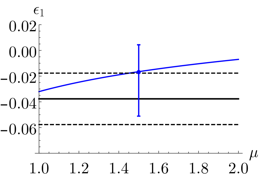
(a)

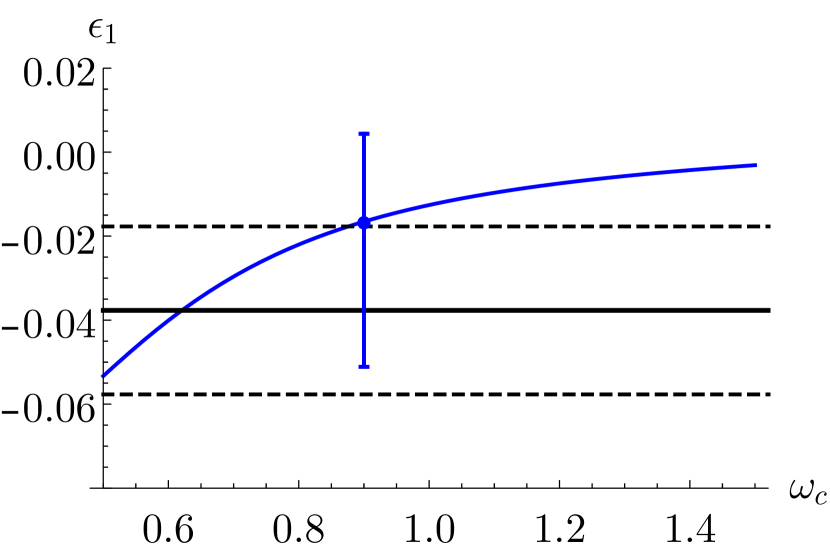
(b)

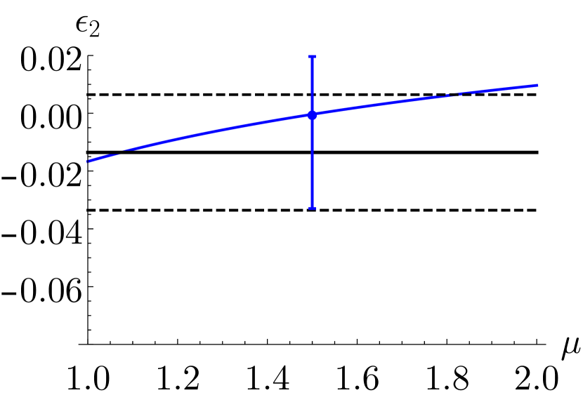
(c)

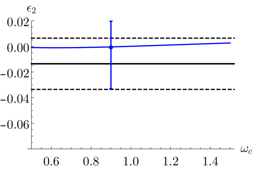
(d)

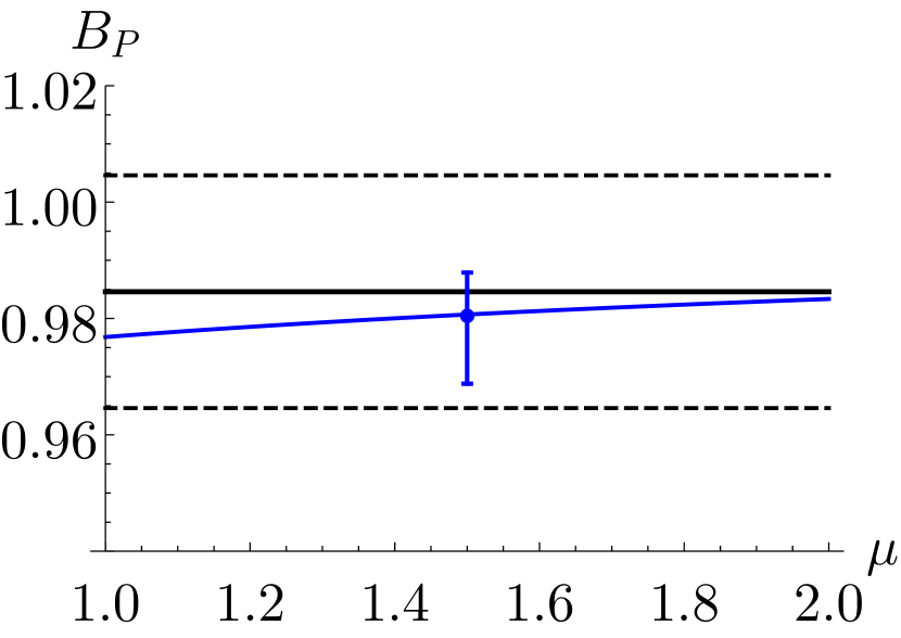
(e)

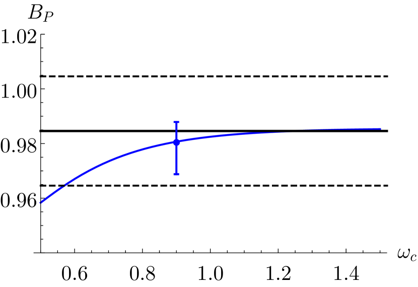
(f)

Figure 4: Comparison of the weight function method (shown in black) to the traditional sum rule approach (shown in blue) for the case of a $B_{d}$ meson. The plots illustrate how the traditional result varies with respect to $\mu$ and $\omega_{c}$ on the left and right respectively. The dashed lines indicate the range of uncertainty in the weight function result, being set to $\pm 0.02$. The blue vertical line indicates our final quoted error for the traditional sum rule method.

Finally we can compare our results with other sum rule analyses of the bag parameters that are available in the literature. The treatment in Ref. [53] shows several key differences compared to ours: in that study, the necessary tools to calculate the dominant perturbative 3-loop non-factorisable contributions shown in Fig. 1 were not yet available. However, additional non-factorisable effects do arise from their procedure for extracting the continuum cut-off, which in their case is not treated as common between the 3-point and 2-point correlators. The main result of that paper is quoted at the scale $m_{b}$, for which there is significant mixing between the bag parameters after running from the hadronic scale. It should also be noted that their results differ from our own by a factor of $F^{2}(m_{b})/F^{2}(\mu)$ due to different conventions in our definition of the matrix elements, (see Eq.(2.3)).

The latest preliminary estimates of the lifetime bag parameters with lattice QCD were obtained 20 years ago in Ref. [24] and so an updated analysis would be greatly appreciated. Comparing those values to our own we find a similar degree of precision for the $\epsilon_{i}$ parameters, while our predictions for the $B_{i}$ have a much smaller range of uncertainty and we disagree with the low value quoted for $B_{2}$.

4 Conclusion

In this work, we have presented an updated sum rule analysis of the $\Delta B=0$ bag parameters in the HQET limit which includes SU(3) flavour breaking effects for the first time, relying on the expansion by regions approach we introduced in our earlier work [25] in the context of $B$-meson mixing. The presence of the eye-contraction diagrams and the mixing between operators of different dimensions in full QCD however poses an additional challenge. For this reason, we work exclusively in HQET where no such mixing occurs. Therefore, the results presented here are also applicable to the $\Delta D=0$ matrix elements (see Ref. [36] for a recent update of $D$ meson lifetimes). In addition, taking this limit leads us to find relatively small uncertainties for the bag parameters themselves since all $1/m_{Q}$ corrections reside in $\tilde{\Gamma}_{7}$ of Eq.(1.1).

The eye contractions are first addressed in this work and also lead to a number of new effects. First of all, their renormalization requires the inclusion of the penguin operator $Q_{P}$ in our operator basis. Furthermore, since the light-quarks $q^{\prime}$ in the operators are not contracted with the light valence quarks $q$ in the mesons, they generate non-valence matrix elements $\delta_{i}^{q^{\prime}q}$ for $q\neq q^{\prime}$. We find that the weight-function method we employed in [25] cannot be used with the non-valence matrix elements due to logarithmic divergences whose origin is discussed in Appendix C. Thus, we adopted the traditional sum rule approach where the Borel parameter and the continuum cutoff are varied in our analysis. We note however that we obtain good consistency between the two methods when they are applied to the tree contractions as shown in Figure 4.

Numerically, we find that deviations from the VSA at the hadronic scale are generally small. The $\mathcal{O}(1)$ uncertainties in the sum rule for the deviations are therefore quite small in absolute terms and sufficient for a phenomenological analysis of the $\tau(B_{s})/\tau(B_{d})$ lifetime ratio, which also requires taking into account the contribution of the Darwin operator [31, 32, 33] and is thus beyond the scope of this work.

Appendix A RGE

To determine the counterterm contribution to the three-point correlator (2.8) we require the one-loop renormalization of the operators (2.1). We obtain the structure

$$\gamma_{\tilde{O}^{q^{\prime}}\tilde{O}^{q}}=\delta_{qq^{\prime}}\gamma_{\tilde{O}\tilde{O}}+\gamma_{\tilde{O}^{\prime}\tilde{O}}$$ (A.1)

with

$$\tilde{\gamma}_{\tilde{O}\tilde{O}}^{(0)}=\left(\begin{array}[]{ccccc}\frac{3}{N_{c}}-3N_{c}&0&6&0&0\\ \vspace*{0.1cm}\par 0&\frac{3}{N_{c}}-3N_{c}&0&6&0\\ \vspace*{0.1cm}\par\frac{3}{2}-\frac{3}{2N_{c}^{2}}&0&-\frac{3}{N_{c}}&0&0\\ \vspace*{0.1cm}\par 0&\frac{3}{2}-\frac{3}{2N_{c}^{2}}&0&-\frac{3}{N_{c}}&0\\ \vspace*{0.1cm}\par 0&0&0&0&-3N_{c}\end{array}\right),$$ (A.2)

and

$$\tilde{\gamma}_{\tilde{O}^{\prime}\tilde{O}}^{(0)}=\left(\begin{array}[]{ccccc}0&0&0&0&\frac{8}{3}\\ \vspace*{0.1cm}\par 0&0&0&0&-\frac{4}{3}\\ \vspace*{0.1cm}\par 0&0&0&0&-\frac{4}{3N_{c}}\\ \vspace*{0.1cm}\par 0&0&0&0&\frac{2}{3N_{c}}\\ \vspace*{0.1cm}\par 0&0&0&0&\frac{4}{3}\par\end{array}\right),$$ (A.3)

The renormalized correlator then takes the form

$$K_{\tilde{Q}_{i}^{q^{\prime}}}^{q,(1)}=K_{\tilde{Q}_{i}^{q^{\prime}}}^{q,(1),\text{bare}}+\frac{1}{2\epsilon}\left[\left(2\tilde{\gamma}_{\tilde{j}}^{(0)}\delta_{ij}+\tilde{\gamma}_{\tilde{Q}_{i}\tilde{Q}_{j}}^{(0)}\right)K_{\tilde{Q}_{j}^{q^{\prime}}}^{q,(0)}+\tilde{\gamma}_{\tilde{Q}_{i}\tilde{E}_{j}}^{(0)}K_{\tilde{E}_{j}^{q^{\prime}}}^{q,(0)}\right]+\frac{1}{2\epsilon}\tilde{\gamma}_{\tilde{Q}_{i}^{\prime}\tilde{Q}_{P}}^{(0)}K_{\tilde{Q}_{P}^{q}}^{q,(0)},$$ (A.4)

where the second term is the counterterm for the tree-level contractions and the third term is the counterterm for the eye contractions.

Now, we consider the RGE for the Bag parameters. We have

$$\frac{d\tilde{\mathbf{O}}^{q^{\prime}}}{d\ln\mu}=-\sum_{q}\tilde{\gamma}_{\tilde{O}^{q^{\prime}}\tilde{O}^{q}}\tilde{\mathbf{O}}^{q}\,,\hskip 28.45274pt\frac{dF_{q}(\mu)}{d\ln\mu}=-\tilde{\gamma}_{\tilde{j}}F_{q}(\mu)\,,$$ (A.5)

and thus obtain the following RGE for the Bag parameters in the case with two light-quark flavors $q$ and $s$:

$$\frac{d}{d\ln\mu}\left(\begin{array}[]{c}\tilde{\mathcal{B}}_{i}^{q}\\ \tilde{\delta}_{i}^{qs}\end{array}\right)=-\frac{\tilde{A}_{j}}{\tilde{A}_{i}}\left(\begin{array}[]{cc}\tilde{\gamma}_{\tilde{O}_{i}\tilde{O}_{j}}+\tilde{\gamma}_{\tilde{O}_{i}^{\prime}\tilde{O}_{j}}-2\tilde{\gamma}_{\tilde{j}}\delta_{ij}&\tilde{\gamma}_{\tilde{O}_{i}^{\prime}\tilde{O}_{j}}\\ \tilde{\gamma}_{\tilde{O}_{i}^{\prime}\tilde{O}_{j}}&\tilde{\gamma}_{\tilde{O}_{i}^{\prime}\tilde{O}_{j}}-2\tilde{\gamma}_{\tilde{j}}\delta_{ij}\end{array}\right)\left(\begin{array}[]{c}\tilde{\mathcal{B}}_{j}^{q}\\ \tilde{\delta}_{j}^{qs}\end{array}\right)\,,$$ (A.6)

which can be easily generalised to more than two quark flavours.

Appendix B Condensate Calculation

Here we lay out as an example our steps to derive the double discontinuity of the non-factorisable gluon-gluon condensate term. Specifically, this example concerns the case of the 3-point function with a penguin operator insertion but, other than alterations to the Dirac structure stemming from the choice of operator, the process is identical for the rest of the operator basis. For the sake of brevity, we take the case of a massless light quark. Following from the procedure described in Ref. [55] we work in the Fock-Schwinger gauge [66, 67],

$$(x-x_{0})A_{\mu}^{a}=0$$ (B.1)

where $x_{0}$ can be set to zero without loss of generality as its dependence drops out of any gauge-invariant quantity. After Wick contracting the fields, the correlator in Eq.(2.8) takes the form,

$$K_{\tilde{Q}_{P}}(\omega_{1},\omega_{2})=-\int[dk]\frac{\text{Tr}\left[\gamma^{5}(1+\not{v})\gamma_{\mu}(1+\not{v})\gamma^{5}S_{ij}(-k_{2})\gamma^{\mu}S_{kl}(-k_{1})\right]}{(-2(k_{1}\cdot v+\omega_{1}))(-2(k_{2}\cdot v+\omega_{1}))}\,T^{a}_{jk}T^{a}_{li}$$ (B.2)

where we define our integral measure as $[dk]\equiv d^{d}k_{1}d^{d}k_{2}/(2\pi)^{2d}$ and it is explicit that we choose to work in momentum space. In Eq.(B.2) we have ignored the contribution from the eye-contraction term since condensate corrections to such diagrams are vanishing at the order considered in this paper (see discussion in Section 2.4). Furthermore, in Eq.(B.2) and in what follows, we drop the notation indicating the flavour of the light quarks appearing in the operator and in the pseudoscalar currents since for this example we take $q=q^{\prime}$ and without mass corrections the result for $u/d$ is identical. The appearance of the gluon-gluon condensate arises from the next to leading order terms in the expansion of the the light quark propagators,

$$\begin{split}S_{ij}(-k)&=S^{(0)}(-k)\delta_{ij}+\frac{ig}{2}\int d^{4}p\,S^{(0)}(-k)G^{b}_{\rho\alpha}(0)T^{b}_{ij}\gamma^{\alpha}\frac{\partial}{\partial p_{\rho}}\delta^{(4)}(p)S^{(0)}(-k-p)+\mathcal{O}(g^{2})\\ &\simeq S^{(0)}(-k)+\frac{ig}{2}S^{(0)}(-k)G^{b}_{\rho\alpha}(0)T^{b}_{ij}\gamma^{\alpha}\left.\frac{\partial S^{(0)}(-k-p)}{\partial p_{\rho}}\right|_{p=0}\end{split}$$ (B.3)

Inserting Eq.(B.3) into Eq.(B.2) and isolating the term in the correlator containing a double insertion of the gluon field strength tensor $G_{\alpha\beta}$, corresponds to the Feynman diagram shown on the left of Fig.2. Applying the partial derivatives,

$$\begin{split}\left.\frac{\partial S^{(0)}(-k-p)}{\partial p_{\rho}}\right|_{p=0}&=\left.\frac{\partial}{\partial p_{\rho}}\frac{-\not{k}-\not{p}}{(k+p)^{2}}\right|_{p=0}\\ &=\frac{2k^{\rho}\not{k}}{k^{4}}-\frac{\gamma^{\rho}}{k^{2}}\end{split}$$ (B.4)

and using the relation,

$$\begin{split}G^{b}_{\rho\alpha}(0)\,G^{c}_{\sigma\beta}(0)&=\delta^{bc}\,\frac{(g_{\rho\sigma}g_{\alpha\beta}-g_{\rho\beta}g_{\alpha\sigma})}{d(d-1)(N_{c}^{2}-1)}\,G^{d}_{\mu\nu}(0)G^{d}_{\mu\nu}(0)\end{split}$$ (B.5)

the calculation is then straight forward. After taking the trace we used FIRE [48] and ran an IBP reduction. The latter step is not necessary but it does provide us with the compact result,

$$K^{\braket{GG}}_{\tilde{Q}_{P}}(\omega_{1},\omega_{2})=-\frac{4(-3+d)^{2}(2-3d+d^{2})}{\omega_{1}\omega_{2}}I(\omega_{1})I(\omega_{2})\frac{1}{4N_{c}\,d(d-1)}\braket{\frac{\alpha_{s}}{\pi}GG}$$ (B.6)

where $I(\omega)$ is a 1-loop HQET integral expressible in terms of Gamma functions,

$$I(\omega)=\frac{i}{(4\pi)^{d/2}}\,(2\omega)^{1-2\epsilon}\Gamma(1-\epsilon)\Gamma(2\epsilon-1)$$ (B.7)

In order to use this in our calculation of the bag parameters, we then take the double discontinuity of the correlator and arrive at,

$$\begin{split}\rho^{\braket{GG}}_{\tilde{Q}_{P}}&=(e^{4\pi i\epsilon}+e^{-4\pi i\epsilon}-2)\frac{K^{\braket{GG}}_{\tilde{Q}_{P}}(\omega_{1},\omega_{2})}{(2\pi i)^{2}}\\ &=\frac{\braket{\frac{\alpha_{s}}{\pi}GG}}{384\pi^{2}}\end{split}$$ (B.8)

Appendix C On the logarithmic divergence at $x=1$

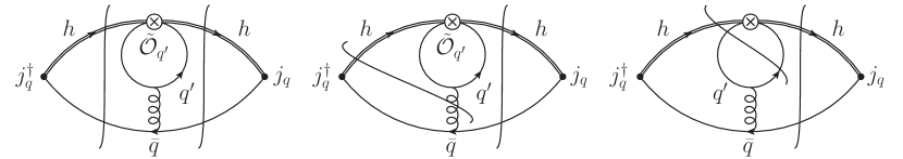
Figure 5: Cuts which yield contributions to the double discontinuity. Symmetric diagrams are not shown.

To investigate the origin of the logarithmic divergences in the results (2.28) for the eye contractions, we study the cuts of the relevant diagram which are contributing to the double discontinuity (see Figure 5). To simplify the discussion in this appendix we only consider the scalar diagram and only work to the first order in $\epsilon$ where such a logarithm appears, but we retain the full strange-quark mass dependence in the penguin loop. Our results for the cuts (assuming $\omega_{2}>\omega_{1}$, denoted by $S_{l}$, $S_{m}$ and $S_{r}$ in this order for the three diagrams) are

$$S_{l}={} \prod_{j=1}^{3}\left(\int\frac{d^{d}k_{j}}{i\pi^{d/2}}\right)\frac{(-2\pi i)^{4}\delta(2\omega_{1}-2v\cdot k_{1})\delta(2\omega_{2}-2v\cdot k_{2})\delta_{+}(k_{1}^{2})\delta_{+}(k_{2}^{2})}{(k_{1}-k_{2})^{2}[k_{3}^{2}-m_{s}^{2}][(k_{3}+k_{2}-k_{1})^{2}-m_{s}^{2}]}$$

$$={} \frac{2\pi^{3}\Gamma(\epsilon)\Gamma(-\epsilon)}{\Gamma(1/2-\epsilon)\Gamma(1-\epsilon)\Gamma(3/2-\epsilon)\omega_{1}^{2\epsilon}\omega_{2}^{2\epsilon}m_{s}^{2\epsilon}}+\mathcal{O}(\epsilon^{0})\,,$$ (C.1)

$$S_{m}={} \prod_{j=1}^{3}\left(\int\frac{d^{d}k_{j}}{i\pi^{d/2}}\right)\frac{(-2\pi i)^{4}\delta(2\omega_{1}-2v\cdot k_{1})\delta(2\omega_{2}-2v\cdot(k_{1}+k_{2}))\delta_{+}(k_{1}^{2})\delta_{+}(k_{2}^{2})}{(k_{1}+k_{2})^{2}[k_{3}^{2}-m_{s}^{2}][(k_{3}+k_{2})^{2}-m_{s}^{2}]}$$

$$={} -\frac{2\pi^{3}\Gamma(\epsilon)\Gamma(-\epsilon)}{\Gamma(1/2-\epsilon)\Gamma(1-\epsilon)\Gamma(3/2-\epsilon)\omega_{1}^{2\epsilon}(\omega_{2}-\omega_{1})^{2\epsilon}m_{s}^{2\epsilon}}\,,$$ (C.2)

$$S_{r}={} \prod_{j=1}^{3}\left(\int\frac{d^{d}k_{j}}{i\pi^{d/2}}\right)\frac{(-2\pi i)^{5}\delta(2\omega_{1}-2v\cdot k_{1})\delta(2\omega_{2}-2v\cdot(k_{1}+k_{2}))}{k_{2}^{2}(k_{1}+k_{2})^{2}}$$

$$\times\delta_{+}(k_{1}^{2})\delta_{+}(k_{3}^{2}-m_{s}^{2})\delta_{+}((k_{2}+k_{3})^{2}-m_{s}^{2})$$

$$={} \mathcal{O}(\epsilon^{0})\,.$$ (C.3)

Summing up these contributions, we find at the first non-vanishing order

$$\left.S_{l}+S_{m}+S_{r}\right|_{\omega_{2}>\omega_{1}}=-\frac{8\pi^{2}}{\epsilon}\ln\left(1-\frac{\omega_{1}}{\omega_{2}}\right)+\mathcal{O}(\epsilon^{0})\,,$$ (C.4)

which diverges logarithmically as $\omega_{1}\to\omega_{2}$. We reproduced this result by using our setup described in Section 2.3 to first compute the scalar diagram and then taking its double discontinuity. To understand this behaviour, we first note that the external momentum $p_{2}-p_{1}$ at the four-quark operator is assumed to be light-like and thus vanishes when $\omega_{1}=\omega_{2}$. Thus, in this limit the process between the two cuts in the diagram in the middle of Figure 5 therefore reduces to the amplitude with two external eikonal lines and one massless line which are all on-shell and is not kinematically allowed. On the other hand the processes between the two cuts of the other diagrams reduce to amplitudes with four external on-shell legs, which are kinematically possible. We further note that both the left and middle diagrams contain collinear divergences which cancel between the leading poles of both contributions, but generate the logarithms at sub-leading orders. Examining the diagrams in the ’tree’ contributions, we find that there are no double-cuts which yield processes that are kinematically forbidden in the limit $\omega_{1}\to\omega_{2}$, which explains why the logarithmic divergences are only found in the ’eye’ contributions. This behaviour is reminiscent of large threshold logarithms that e.g. arise in Higgs production, where infrared $1/\epsilon$ poles cancel in the sum of real and virtual corrections, but large logarithms appear because the real corrections are phase-space suppressed near the threshold. Interestingly though, the logarithms we observe here appear to be of collinear rather than soft origin.

Appendix D $F_{q}$ and $\overline{\Lambda}_{q}$ analysis

For the discontinuity $\rho_{\Pi}(\omega)$ needed to form the sum rule of the HQET decay constant, we use the NLO result computed in Ref. [42] along with the $m_{s}$ expanded result computed in Ref. [25],

$$\rho_{\Pi}(\omega) \equiv \frac{\Pi(\omega+i0)-\Pi(\omega-i0)}{2\pi i}$$

$$= \frac{N_{c}\omega^{2}}{2\pi^{2}}\,\theta(\omega-m_{s})\Bigg{\{}1+\frac{m_{s}}{\omega}-\frac{1}{2}\,\left(\frac{m_{s}}{\omega}\right)^{2}+\dots$$

$$+\frac{\alpha_{s}C_{F}}{4\pi}\,\Bigg{[}17+\frac{4\pi^{2}}{3}+3\ln\frac{\mu_{\rho}^{2}}{4\omega^{2}}+\left(20+\frac{4\pi^{2}}{3}+6\ln\frac{\mu_{\rho}^{2}}{4\omega^{2}}-3\ln\frac{\mu_{\rho}^{2}}{m_{s}^{2}}\right)\,\frac{m_{s}}{\omega}$$

$$+\left(1-\frac{9}{2}\ln\frac{\mu_{\rho}^{2}}{4\omega^{2}}+3\ln\frac{\mu_{\rho}^{2}}{m_{s}^{2}}\right)\,\left(\frac{m_{s}}{\omega}\right)^{2}+\dots\Bigg{]}+\mathcal{O}(\alpha_{s}^{2})\Bigg{\}}$$

$$-\frac{\langle\bar{s}s\rangle}{2}\delta(\omega)\left[1+6\frac{\alpha_{s}C_{F}}{4\pi}+\mathcal{O}(\alpha_{s}^{2})\right]+\frac{\langle\bar{s}i\sigma_{\mu\nu}G^{\mu\nu}s\rangle}{32}\delta^{\prime\prime}(\omega)\left[1+\mathcal{O}(\alpha_{s})\right]+\mathcal{O}(\Lambda^{6}).$$

After plugging Eq.(D) into Eq.(2.7), logarithmic terms of the form $\log(\mu^{2}/m_{s}^{2})$ can be resummed by switching to the $\overline{\text{MS}}$ scheme,

$$m_{s}=\bar{m}_{s}(\mu_{\rho})\left[1+\frac{\alpha_{s}(\mu_{\rho})C_{F}}{4\pi}\left(4+3\log\left(\frac{\mu_{\rho}^{2}}{\bar{m}_{s}^{2}(\mu_{\rho})}\right)\right)+\dots\right]\,.$$ (D.3)

We also note that $m_{s}$ terms arising from the lower integration cut in Eq.(2.7) were not expanded in $m_{s}$.

The running of the quark condensates takes the form [see Ref. [41]]

$$\langle\bar{s}s\rangle(\mu_{\rho}) =\langle\bar{s}s\rangle(\mu_{0})\left[\frac{\alpha_{s}(\mu_{\rho})}{\alpha_{s}(\mu_{0})}\right]^{\frac{\gamma_{0}^{(3)}}{2\beta_{0}}}\times\left[1+\frac{\alpha_{s}(\mu_{\rho})-\alpha_{s}(\mu_{0})}{4\pi}\frac{\gamma_{0}^{(3)}}{2\beta_{0}}\left(\frac{\gamma_{1}^{(3)}}{\gamma_{0}^{(3)}}-\frac{\beta_{1}}{\beta_{0}}\right)\right]\,,$$

$$\langle\bar{s}i\sigma_{\mu\nu}G^{\mu\nu}s\rangle(\mu_{\rho}) =\langle\bar{s}i\sigma_{\mu\nu}G^{\mu\nu}s\rangle(\mu_{0})\left[\frac{\alpha_{s}(\mu_{\rho})}{\alpha_{s}(\mu_{0})}\right]^{\frac{\gamma_{0}^{(5)}}{2\beta_{0}}}\,,$$ (D.4)

with $\gamma_{0}^{(3)}=-8$, $\gamma_{0}^{(5)}=-4/3$, $\gamma_{1}^{(3)}=-404/3+40n_{f}/9$, $\beta_{0}=11-2n_{f}/3$ and $\beta_{1}=102-38n_{f}/3$. The logarithmic derivative of Eq.(2.7) furthermore gives us a sum rule for the mass difference $\overline{\Lambda}_{s}$ in the form [see Ref. [41]]

$$\overline{\Lambda}=t^{2}\frac{\frac{d}{dt}\int\limits_{0}^{\omega_{c}}d\omega\,e^{-\frac{\omega}{t}}\rho_{\Pi}(\omega)}{\int\limits_{0}^{\omega_{c}}d\omega\,e^{-\frac{\omega}{t}}\rho_{\Pi}(\omega)}=\frac{\int\limits_{0}^{\omega_{c}}d\omega\,\omega\,e^{-\frac{\omega}{t}}\rho_{\Pi}(\omega)}{\int\limits_{0}^{\omega_{c}}d\omega\,e^{-\frac{\omega}{t}}\rho_{\Pi}(\omega)}\,.$$ (D.5)

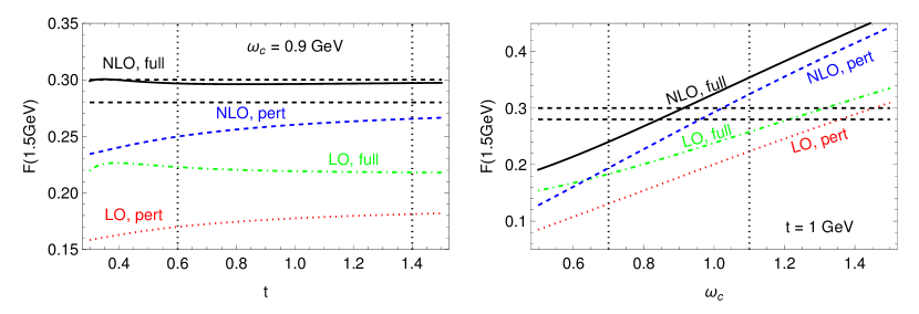
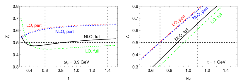
Figure 6: Dependence of the sum rule results for $F(\mu)$ (top) and $\overline{\Lambda}$ (bottom) on the Borel parameter $t$ (left) and the continuum cutoff $\omega_{c}$ (right) in the $B_{q}$ system.

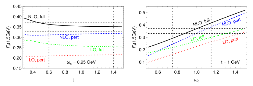
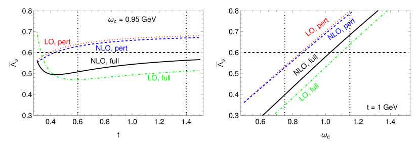
Figure 7: Dependence of the sum rule results for $F_{s}(\mu)$ (top) and $\overline{\Lambda}_{s}$ (bottom) on the Borel parameter $t$ (left) and the continuum cutoff $\omega_{c}$ (right) in the $B_{s}$ system.

To determine the appropriate ranges for the Borel parameters $t_{i}$ and the continuum cutoff $\omega_{c}$ in our bag parameter analysis, we consider the sum rules for the meson-heavy quark mass difference $\overline{\Lambda}_{q}$ and the HQET decay constant $F$ and compare with the values found in the literature. The values of the HQET decay constants,

$$F(1.5\,\text{GeV})=(0.29\pm 0.01)\,\text{GeV}\,,\hskip 28.45274ptF_{s}(1.5\,\text{GeV})=(0.35\pm 0.02)\,\text{GeV}\,,$$ (D.6)

are determined from the static results of the ALPHA collaboration from Ref. [68] by matching at the scale $\bar{m}_{b}(\bar{m}_{b})$ and evolving the HQET decay constants down to the scale 1.5GeV. For the mass differences we use, $\overline{\Lambda}_{q}=0.5$ and $\overline{\Lambda}_{s}=0.6$ for the $B_{q}$ and $B_{s}$ mesons respectively. We find the behaviour shown in Figures 6 and 7 from which we determine the following intervals:

$$B_{q}: \hskip 28.45274ptt=(1.0\pm 0.4)\,\text{GeV}\,,\hskip 14.22636pt\omega_{c}=(0.90\pm 0.2)\,\text{GeV}\,,$$

$$B_{s}: \hskip 28.45274ptt=(1.0\pm 0.4)\,\text{GeV}\,,\hskip 14.22636pt\omega_{c}=(0.95\pm 0.2)\,\text{GeV}\,.$$ (D.7)

References

- [1] HFLAV collaboration, Y. S. Amhis et al., Averages of -hadron, -hadron, and -lepton properties as of 2018, 1909.12524.
- [2] M. Kirk, A. Lenz and T. Rauh, Dimension-six matrix elements for meson mixing and lifetimes from sum rules, JHEP 12 (2017) 068, [1711.02100].
- [3] LHCb collaboration, R. Aaij et al., Measurement of the -violating phase from decays in 13 TeV collisions, Phys. Lett. B 797 (2019) 134789, [1903.05530].
- [4] LHCb collaboration, R. Aaij et al., Updated measurement of time-dependent CP-violating observables in decays, Eur. Phys. J. C 79 (2019) 706, [1906.08356].
- [5] ATLAS collaboration, G. Aad et al., Measurement of the -violating phase in decays in ATLAS at 13 TeV, Eur. Phys. J. C 81 (2021) 342, [2001.07115].
- [6] CMS collaboration, A. M. Sirunyan et al., Measurement of the -violating phase in the B J(1020) K+K- channel in proton-proton collisions at 13 TeV, Phys. Lett. B 816 (2021) 136188, [2007.02434].
- [7] A. Lenz, Theory Motivation: What measurements are needed?, in 15th International Conference on Heavy Quarks and Leptons, 10, 2021. 2110.01662.
- [8] V. A. Khoze and M. A. Shifman, HEAVY QUARKS, Sov. Phys. Usp. 26 (1983) 387.
- [9] M. A. Shifman and M. B. Voloshin, Preasymptotic Effects in Inclusive Weak Decays of Charmed Particles, Sov. J. Nucl. Phys. 41 (1985) 120.
- [10] I. I. Y. Bigi and N. G. Uraltsev, Gluonic enhancements in non-spectator beauty decays: An Inclusive mirage though an exclusive possibility, Phys. Lett. B 280 (1992) 271–280.
- [11] I. I. Y. Bigi, N. G. Uraltsev and A. I. Vainshtein, Nonperturbative corrections to inclusive beauty and charm decays: QCD versus phenomenological models, Phys. Lett. B 293 (1992) 430–436, [hep-ph/9207214].
- [12] B. Blok and M. A. Shifman, The Rule of discarding 1/N(c) in inclusive weak decays. 1., Nucl. Phys. B 399 (1993) 441–458, [hep-ph/9207236].
- [13] B. Blok and M. A. Shifman, The Rule of discarding 1/N(c) in inclusive weak decays. 2., Nucl. Phys. B 399 (1993) 459–476, [hep-ph/9209289].
- [14] J. Chay, H. Georgi and B. Grinstein, Lepton energy distributions in heavy meson decays from QCD, Phys. Lett. B 247 (1990) 399–405.
- [15] M. E. Luke, Effects of subleading operators in the heavy quark effective theory, Phys. Lett. B 252 (1990) 447–455.
- [16] I. I. Y. Bigi, B. Blok, M. A. Shifman, N. G. Uraltsev and A. I. Vainshtein, A QCD ’manifesto’ on inclusive decays of beauty and charm, in 7th Meeting of the APS Division of Particles Fields, pp. 610–613, 11, 1992. hep-ph/9212227.
- [17] A. Lenz, Lifetimes and heavy quark expansion, Int. J. Mod. Phys. A 30 (2015) 1543005, [1405.3601].
- [18] N. G. Uraltsev, On the problem of boosting nonleptonic b baryon decays, Phys. Lett. B 376 (1996) 303–308, [hep-ph/9602324].
- [19] M. Neubert and C. T. Sachrajda, Spectator effects in inclusive decays of beauty hadrons, Nucl. Phys. B 483 (1997) 339–370, [hep-ph/9603202].
- [20] M. Beneke, G. Buchalla, C. Greub, A. Lenz and U. Nierste, The Lifetime Difference Beyond Leading Logarithms, Nucl. Phys. B 639 (2002) 389–407, [hep-ph/0202106].
- [21] E. Franco, V. Lubicz, F. Mescia and C. Tarantino, Lifetime ratios of beauty hadrons at the next-to-leading order in QCD, Nucl. Phys. B 633 (2002) 212–236, [hep-ph/0203089].
- [22] M. Ciuchini, E. Franco, V. Lubicz and F. Mescia, Next-to-leading order QCD corrections to spectator effects in lifetimes of beauty hadrons, Nucl. Phys. B 625 (2002) 211–238, [hep-ph/0110375].
- [23] Y.-Y. Keum and U. Nierste, Probing penguin coefficients with the lifetime ratio tau (B-s) / tau (B-d), Phys. Rev. D 57 (1998) 4282–4289, [hep-ph/9710512].
- [24] D. Becirevic, Theoretical progress in describing the B meson lifetimes, PoS HEP2001 (2001) 098, [hep-ph/0110124].
- [25] D. King, A. Lenz and T. Rauh, Bs mixing observables and —Vtd/Vts— from sum rules, JHEP 05 (2019) 034, [1904.00940].
- [26] L. Di Luzio, M. Kirk, A. Lenz and T. Rauh, theory precision confronts flavour anomalies, JHEP 12 (2019) 009, [1909.11087].
- [27] Fermilab Lattice, MILC collaboration, A. Bazavov et al., -mixing matrix elements from lattice QCD for the Standard Model and beyond, Phys. Rev. D 93 (2016) 113016, [1602.03560].
- [28] RBC/UKQCD collaboration, P. A. Boyle, L. Del Debbio, N. Garron, A. Juttner, A. Soni, J. T. Tsang et al., SU(3)-breaking ratios for and mesons, 1812.08791.
- [29] R. J. Dowdall, C. T. H. Davies, R. R. Horgan, G. P. Lepage, C. J. Monahan, J. Shigemitsu et al., Neutral B-meson mixing from full lattice QCD at the physical point, Phys. Rev. D 100 (2019) 094508, [1907.01025].
- [30] L. Di Luzio, M. Kirk and A. Lenz, Updated -mixing constraints on new physics models for anomalies, Phys. Rev. D 97 (2018) 095035, [1712.06572].
- [31] A. Lenz, M. L. Piscopo and A. V. Rusov, Contribution of the Darwin operator to non-leptonic decays of heavy quarks, JHEP 12 (2020) 199, [2004.09527].
- [32] T. Mannel, D. Moreno and A. Pivovarov, Heavy quark expansion for heavy hadron lifetimes: completing the corrections, JHEP 08 (2020) 089, [2004.09485].
- [33] D. Moreno Torres, Completing corrections to non-leptonic bottom-to-up-quark decays, JHEP 01 (2021) 051, [2009.08756].
- [34] A. Alberti, P. Gambino, K. J. Healey and S. Nandi, Precision Determination of the Cabibbo-Kobayashi-Maskawa Element , Phys. Rev. Lett. 114 (2015) 061802, [1411.6560].
- [35] M. Bordone, B. Capdevila and P. Gambino, Three loop calculations and inclusive Vcb, Phys. Lett. B 822 (2021) 136679, [2107.00604].
- [36] D. King, A. Lenz, M. L. Piscopo, T. Rauh, A. V. Rusov and C. Vlahos, Revisiting Inclusive Decay Widths of Charmed Mesons, 2109.13219.
- [37] Particle Data Group collaboration, P. A. Zyla et al., Review of Particle Physics, PTEP 2020 (2020) 083C01.
- [38] Belle-II collaboration, F. Abudinén et al., Precise measurement of the and lifetimes at Belle II, 2108.03216.
- [39] A. Lenz and T. Rauh, D-meson lifetimes within the heavy quark expansion, Phys. Rev. D 88 (2013) 034004, [1305.3588].
- [40] M. Neubert, Heavy meson form-factors from QCD sum rules, Phys. Rev. D 45 (1992) 2451–2466.
- [41] E. Bagan, P. Ball, V. M. Braun and H. G. Dosch, QCD sum rules in the effective heavy quark theory, Phys. Lett. B 278 (1992) 457–464.
- [42] D. J. Broadhurst and A. G. Grozin, Operator product expansion in static quark effective field theory: Large perturbative correction, Phys. Lett. B 274 (1992) 421–427, [hep-ph/9908363].
- [43] E. V. Shuryak, Hadrons Containing a Heavy Quark and QCD Sum Rules, Nucl. Phys. B 198 (1982) 83–101.
- [44] M. Jamin and M. E. Lautenbacher, TRACER: Version 1.1: A Mathematica package for gamma algebra in arbitrary dimensions, Comput. Phys. Commun. 74 (1993) 265–288.
- [45] S. A. Larin, The Renormalization of the axial anomaly in dimensional regularization, Phys. Lett. B 303 (1993) 113–118, [hep-ph/9302240].
- [46] P. Nogueira, Automatic Feynman graph generation, J. Comput. Phys. 105 (1993) 279–289.
- [47] K. G. Chetyrkin and F. V. Tkachov, Integration by Parts: The Algorithm to Calculate beta Functions in 4 Loops, Nucl. Phys. B 192 (1981) 159–204.
- [48] A. V. Smirnov, FIRE5: a C++ implementation of Feynman Integral REduction, Comput. Phys. Commun. 189 (2015) 182–191, [1408.2372].
- [49] A. G. Grozin and R. N. Lee, Three-loop HQET vertex diagrams for B0 - anti-B0 mixing, JHEP 02 (2009) 047, [0812.4522].
- [50] T. Huber and D. Maitre, HypExp 2, Expanding Hypergeometric Functions about Half-Integer Parameters, Comput. Phys. Commun. 178 (2008) 755–776, [0708.2443].
- [51] M. Beneke and V. A. Smirnov, Asymptotic expansion of Feynman integrals near threshold, Nucl. Phys. B 522 (1998) 321–344, [hep-ph/9711391].
- [52] B. Jantzen, Foundation and generalization of the expansion by regions, JHEP 12 (2011) 076, [1111.2589].
- [53] H.-Y. Cheng and K.-C. Yang, Nonspectator effects and meson lifetimes from a field theoretic calculation, Phys. Rev. D 59 (1999) 014011, [hep-ph/9805222].
- [54] M. S. Baek, J. Lee, C. Liu and H. S. Song, Four quark operators relevant to B meson lifetimes from QCD sum rules, Phys. Rev. D 57 (1998) 4091–4096, [hep-ph/9709386].
- [55] V. A. Novikov, M. A. Shifman, A. I. Vainshtein and V. I. Zakharov, Calculations in External Fields in Quantum Chromodynamics. Technical Review, Fortsch. Phys. 32 (1984) 585.
- [56] L. J. Reinders, H. Rubinstein and S. Yazaki, Hadron Properties from QCD Sum Rules, Phys. Rept. 127 (1985) 1.
- [57] P. Pascual and R. Tarrach, QCD: RENORMALIZATION FOR THE PRACTITIONER, vol. 194. 1984.
- [58] F. Herren and M. Steinhauser, Version 3 of RunDec and CRunDec, Comput. Phys. Commun. 224 (2018) 333–345, [1703.03751].
- [59] V. M. Belyaev and B. L. Ioffe, Determination of Baryon and Baryonic Resonance Masses from QCD Sum Rules. 1. Nonstrange Baryons, Sov. Phys. JETP 56 (1982) 493–501.
- [60] Particle Data Group collaboration, M. Tanabashi et al., Review of Particle Physics, Phys. Rev. D 98 (2018) 030001.
- [61] P. Ball, V. M. Braun and A. Lenz, Higher-twist distribution amplitudes of the K meson in QCD, JHEP 05 (2006) 004, [hep-ph/0603063].
- [62] C. McNeile, A. Bazavov, C. T. H. Davies, R. J. Dowdall, K. Hornbostel, G. P. Lepage et al., Direct determination of the strange and light quark condensates from full lattice QCD, Phys. Rev. D 87 (2013) 034503, [1211.6577].
- [63] HPQCD collaboration, C. T. H. Davies, K. Hornbostel, J. Komijani, J. Koponen, G. P. Lepage, A. T. Lytle et al., Determination of the quark condensate from heavy-light current-current correlators in full lattice QCD, Phys. Rev. D 100 (2019) 034506, [1811.04305].
- [64] M. Beneke, A. Maier, J. Piclum and T. Rauh, The bottom-quark mass from non-relativistic sum rules at NNNLO, Nucl. Phys. B 891 (2015) 42–72, [1411.3132].
- [65] M. Beneke, A. Maier, J. Piclum and T. Rauh, NNNLO determination of the bottom-quark mass from non-relativistic sum rules, PoS RADCOR2015 (2016) 035, [1601.02949].
- [66] V. Fock, Proper time in classical and quantum mechanics, Phys. Z. Sowjetunion 12 (1937) 404–425.
- [67] J. S. Schwinger, On gauge invariance and vacuum polarization, Phys. Rev. 82 (1951) 664–679.
- [68] ALPHA collaboration, F. Bernardoni et al., Decay constants of B-mesons from non-perturbative HQET with two light dynamical quarks, Phys. Lett. B 735 (2014) 349–356, [1404.3590].