Understanding Square Loss in Training Overparametrized Neural Network Classifiers

Abstract

Deep learning has achieved many breakthroughs in modern classification tasks. Numerous architectures have been proposed for different data structures but when it comes to the loss function, the cross-entropy loss is the predominant choice. Recently, several alternative losses have seen revived interests for deep classifiers. In particular, empirical evidence seems to promote square loss but a theoretical justification is still lacking. In this work, we contribute to the theoretical understanding of square loss in classification by systematically investigating how it performs for overparametrized neural networks in the neural tangent kernel (NTK) regime. Interesting properties regarding the generalization error, robustness, and calibration error are revealed. We consider two cases, according to whether classes are separable or not. In the general non-separable case, fast convergence rate is established for both misclassification rate and calibration error. When classes are separable, the misclassification rate improves to be exponentially fast. Further, the resulting margin is proven to be lower bounded away from zero, providing theoretical guarantees for robustness. We expect our findings to hold beyond the NTK regime and translate to practical settings. To this end, we conduct extensive empirical studies on practical neural networks, demonstrating the effectiveness of square loss in both synthetic low-dimensional data and real image data. Comparing to cross-entropy, square loss has comparable generalization error but noticeable advantages in robustness and model calibration.

1 introduction

The pursuit of better classifiers has fueled the progress of machine learning and deep learning research. The abundance of benchmark image datasets, e.g., MNIST, CIFAR, ImageNet, etc., provides test fields for all kinds of new classification models, especially those based on deep neural networks (DNN). With the introduction of CNN, ResNets, and transformers, DNN classifiers are constantly improving and catching up to the human-level performance. In contrast to the active innovations in model architecture, the training objective remains largely stagnant, with cross-entropy loss being the default choice. Despite its popularity, cross-entropy has been shown to be problematic in some applications. Among others, Yu et al. [1] argued that features learned from cross-entropy lack interpretability and proposed a new loss aiming for maximum coding rate reduction. Pang et al. [2] linked the use of cross-entropy to adversarial vulnerability and proposed a new classification loss based on latent space matching. Guo et al. [3] discovered that the confidence of most DNN classifiers trained with cross-entropy is not well-calibrated.

Recently, several alternative losses have seen revived interests for deep classifiers. In particular, many existing works have presented empirical evidence promoting the use of square loss over cross-entropy. Hui and Belkin [4] conducted large-scale experiments comparing the two and found that square loss tends to perform better in natural language processing related tasks while cross-entropy usually yields slightly better accuracy in image classification. Similar comparisons are also made in Demirkaya et al. [5]. Kornblith et al. [6] compared a variety of loss functions and output layer regularization strategies on the accuracy and out-of-distribution robustness, and found that square loss has greater class separation and better out-of-distribution robustness.

In comparison to the empirical investigation, theoretical understanding of square loss in training deep learning classifiers is still lacking. Through our lens, square loss has its uniqueness among classic classification losses, and we argue that it has great potentials for modern classification tasks. Below we list our motivations and reasons why.

Explicit feature modeling Deep learning’s success can be largely attributed to its superior ability as feature extractors. For classification, the ideal features should be separated between classes and concentrated within classes. However, when optimizing cross-entropy loss, it’s not obvious what the learned features should look like [1]. In the terminal stage of training, [7] proved that when cross-entropy is sufficiently minimized, the penultimate layers features will collapse to the scaled simplex structure. Knowing this, would it be better to directly enforce the terminal solution by using square loss with the simplex coding [8]? Unlike cross-entropy, square loss uses the label codings (one-hot, simplex etc.) as features, which can be modeled explicitly to control class separations.

Model Calibration An ideal classifier should not only give the correct class prediction, but also with the correct confidence. Calibration error measures the closeness of the predicted confidence to the underlying conditional probability $\eta$. Using square loss in classification can be essentially viewed as regression where it treats discrete labels as continuous code vectors. It can be shown that the optimal classifier under square loss is $2\eta-1$, linear with the ground truth. This distinguishing property allows it to easily recover $\eta$. In comparison, the optimal classifiers under the hinge loss and cross-entropy are sign$(2\eta-1)$ and $\log(\frac{\eta}{1-\eta})$, respectively. Therefore, hinge loss doesn’t provide reliable information on the prediction confidence, and cross-entropy can be problematic when $\eta$ is close to 0 or 1 [9]. Hence, in terms of model calibration, square loss is a natural choice.

Connections to popular approaches Mixup [10] is a popular data augmentation technique where augmented data are constructed via convex combinations of inputs and their labels. Like in square loss, mixup treats labels as continuous and is shown to improve the generalization of DNN classifiers. In knowledge distillation [11], where a student classifier is trying to learn from a trained teacher, Menon et al. [12] proved that the “optimal" teacher with the ground truth conditional probabilities provides the lowest variance in student learning. Since classifiers trained using square loss is a natural consistent estimator of $\eta$, one can argue that it is a better teacher. In supervised contrastive learning [13], the optimal features are the same as those from square loss with simplex label coding [14] (details in Section 4).

Despite its lack of popularity in practice, square loss has many advantages that can be easily overlooked. In this work, we systematically investigate from a statistical estimation perspective, the properties of deep learning classifiers trained using square loss. The neural networks in our analysis are required to be sufficiently overparametrized in the neural tangent kernel (NTK) regime. Even though this restricts the implication of our results, it is a necessary first step towards a deeper understanding. In summary, our main contributions are:

• Generalization error bound: We consider two cases, according to whether classes are separable or not. In the general non-separable case, we adopt the classical binary classification setting with smooth conditional probability. Fast rate of convergence is established for overparametrized neural network classifiers with Tsybakov’s noise condition. If two classes are separable with positive margins, we show that overparametrized neural network classifiers can provably reach zero misclassification error with probability exponentially tending to one. To the best of our knowledge, this is the first such result for separable but not linear separable classes. Furthermore, we bridge these two cases and offer a unified view by considering auxiliary random noise injection.

• Robustness (margin property): When two classes are separable, the decision boundary is not unique and large-margin classifiers are preferred. In the separable case, we further show that the decision boundary of overparametrized neural network classifiers trained by square loss cannot be too close to the data support and the resulting margin is lower bounded away from zero, providing theoretical guarantees for robustness.

• Calibration error: We show that classifiers trained using square loss are inherently well-calibrated, i.e., the trained classifier provides consistent estimation of the ground-truth conditional probability in $L_{\infty}$ norm. Such property doesn’t hold for cross-entropy.

• Empirical evaluation: We corroborate our theoretical findings with empirical experiments in both synthetic low-dimensional data and real image data. Comparing to cross-entropy, square loss has comparable generalization error but noticeable advantages in robustness and model calibration.

This work contributes to the theoretical understanding of deep classifiers, from a nonparametric estimation point of view, which has been a classic topic in statistics literature. Among others, Mammen and Tsybakov [15] established the optimal convergence rate for 0-1 loss excess risk when the decision boundary is smooth. Zhang [9], Bartlett et al. [16] extended the analysis to various surrogate losses. Audibert and Tsybakov [17], Kohler and Krzyzak [18] studied the convergence rates for plug-in classifiers from local averaging estimators. Steinwart et al. [19] investigated the convergence rate for support vector machine using Gaussian kernels. We build on and extend classic results to neural networks in the NTK regime. There are existing nonparametric results on deep classifiers, e.g., Kim et al. [20] derived fast convergence rates of DNN classifiers that minimize the empirical hinge loss, [21] considered a family of CNN-inspired classifiers and developed similar results for the empirical cross-entropy minimizer, etc. Unlike aforementioned works that only concern the existence of a good classifier (with theoretical worst-case guarantee), in ignorance of the tremendous difficulty of neural network optimization, our results further incorporate the training algorithm and apply to trained classifiers, which relates better to practice. To the best of the authors’ knowledge, similar attainable fast rates (faster than $n^{-\frac{1}{2}}$) have never been established for neural network classifiers.

We require the neural network to be overparametrized, which has been extensively studied recently, under the umbrella term NTK. Most such results are in the regression setting with a handful of exceptions. Ji and Telgarsky [22] showed that only polylogarithmic width is sufficient for gradient descent to overfit the training data using logistic loss. Hu et al. [23] proved generalization error bound for regularized NTK in classification. Cao and Gu [24; 25] provided optimization and generalization guarantees for overparametrized network trained with cross-entropy. In comparison, our results are sharper in the sense that we take the ground truth data assumptions into consideration. This allows a faster convergence rate, especially when the classes are separable, where the exponential convergence rate is attainable. The NTK framework greatly reduces the technical difficulty for our theoretical analysis. However, our results are mainly due to properties of the square loss itself and we expect them to hold for a wide range of classifiers.

There are other works investigating the use of square loss for training (deep) classifiers. Han et al. [26] uncovered that the “neural collapse" phenomenon also occurs under square loss where the last-layer features eventually collapse to their simplex-style class-means. Muthukumar et al. [27] compared classification and regression tasks in the overparameterized linear model with Gaussian features, illustrating different roles and properties of loss functions used at the training and testing phases. Poggio and Liao [28] made interesting observations on effects of popular regularization techniques such as batch normalization and weight decay on the gradient flow dynamics under square loss. These findings support our theoretical results’ implication, which further strengthens our beliefs that the essence comes from the square loss and our analysis can go beyond NTK regime.

The rest of this paper is arranged as follows. Section 2 presents some preliminaries. Main theoretical results are in Section 3. The simplex label coding is discussed in Section 4 followed by numerical studies in Section 5 and conclusions in Section 6. Technical proofs and details of the numerical studies can be found in the Appendix.

2 Preliminaries

Notation For a function $f:\Omega\to\mathbb{R}$, let $\left\lVert f\right\rVert_{\infty}=\sup_{\bm{x}\in\Omega}|f(\bm{x})|$ and $\left\lVert f\right\rVert_{p}=(\int_{\Omega}|f(\bm{x})|^{p}d\bm{x})^{1/p}$. For a vector $\bm{x}$, $\left\lVert\bm{x}\right\rVert_{p}$ denotes its $p$-norm, for $1\leq p\leq\infty$. $L_{p}$ and $l_{p}$ are used to distinguish function norms and vector norms. For two positive sequences $\{a_{n}\}_{n\in\mathbb{N}}$ and $\{b_{n}\}_{n\in\mathbb{N}}$, we write $a_{n}\lesssim b_{n}$ if there exists a constant $C>0$ such that $a_{n}\leq Cb_{n}$ for all sufficiently large $n$. We write $a_{n}\asymp b_{n}$ if $a_{n}\lesssim b_{n}$ and $b_{n}\lesssim a_{n}$. Let $[N]=\{1,\dots,N\}$ for $N\in\mathbb{N}$, $\mathbb{I}$ be the indicator function, and $\bm{I}_{d}$ be the $d\times d$ identity matrix. $N(\mu,\mathbf{\Sigma})$ represents Gaussian distribution with mean $\mu$ and covariance $\mathbf{\Sigma}$.

Classification problem settings Let $P$ be an underlying probability measure on $\Omega\times\bm{Y}$, where $\Omega\subset\mathbb{R}^{d}$ is compact and ${\bm{Y}}=\{1,-1\}$. Let $(X,Y)$ be a random variable with respect to $P$. Suppose we have observations $\{(\bm{x}_{i},y_{i})\}_{i=1}^{n}\subset(\Omega\times Y)^{n}$ i.i.d. sampled according to $P$. The classification task is to predict the unobserved label $y$ given a new input $\bm{x}\in\Omega$. Let $\eta$ defined on $\Omega$ denote the conditional probability, i.e., $\eta(\bm{x})=\mathbb{P}(y=1|\bm{x})$. Let $P_{X}$ be the marginal distribution of $P$ on $X$. The key quantity of interest is the misclassification error, i.e., 0-1 loss. In the population level, the 0-1 loss can be written as

$$L(f)=\mathbb{E}_{(X,Y)\sim P}\mathbb{I}\{{\rm sign}(f(X))\neq Y\}= \mathbb{E}_{X\sim P_{X}}[(1-\eta(X))\mathbb{I}\{f(X)\geq 0\}+\eta(X)\mathbb{I}\{f(X)<0\}],$$ (2.1)

where the expectation is taken with respect to the probability measure $P$. Clearly, an optimal classifier with the minimal 0-1 loss is $2\eta-1$.

According to whether labels are deterministic, there are two scenarios of interest. If $\eta$ only takes values from $\{0,1\}$, i.e., labels are deterministic, we call this case the separable case. Let $\Omega_{1}=\{\bm{x}|\eta(\bm{x})=1\}$, $\Omega_{2}=\{\bm{x}|\eta(\bm{x})=0\}$ and $\Omega=\Omega_{1}\cup\Omega_{2}$. If the probability measure of $\{\bm{x}|\eta(\bm{x})\in(0,1)\}$ is non-zero, i.e., the labels contain randomness, we call this case the non-separable case. In the separable case, we further assume that there exists a positive margin, i.e., dist$(\Omega_{1},\Omega_{2})\geq 2\gamma>0$, where $\gamma$ is a constant, and dist$(\Omega_{1},\Omega_{2})=\inf_{\bm{x}\in\Omega_{1},\bm{x}^{\prime}\in\Omega_{2}}\left\lVert\bm{x}-\bm{x}^{\prime}\right\rVert_{2}$. In the non-separable case, to quantify the difficulty of classification, we adopt the well-established Tsybakov’s noise condition [17], which measures how large the “difficult region” is where $\eta(\bm{x})\approx 1/2$.

Definition 2.1 (Tsybakov’s noise condition).

Let $\kappa\in[0,\infty]$. We say $P$ has Tsybakov noise exponent $\kappa$ if there exists a constant $C,T>0$ such that for all $0<t<T$, $P_{X}(|2\eta(X)-1|<t)\leq C\cdot t^{\kappa}.$

A large value of $\kappa$ implies the difficult region to be small. It is expected that a larger $\kappa$ leads to a faster convergence rate of a neural network classifier. This intuition is verified for the overparametrized neural network classifier trained by square loss and $\ell_{2}$ regularization. See Section 3 for more details.

Neural network setup We mainly focus on the one-hidden-layer ReLU neural network family $\mathcal{F}$ with $m$ nodes in the hidden layer, denoted by

$$f_{\bm{W},\bm{a}}(\bm{x})=\frac{1}{\sqrt{m}}\sum_{r=1}^{m}a_{r}\sigma(\bm{W}_{r}^{\top}\bm{x}),$$

where $\bm{x}\in\Omega$, $\bm{W}=(\bm{W}_{1},\cdots,\bm{W}_{m})\in\mathbb{R}^{d\times m}$ is the weight matrix in the hidden layer, $\bm{a}=(a_{1},\cdots,a_{m})^{\top}\in\mathbb{R}^{m}$ is the weight vector in the output layer, $\sigma(z)=\max\{0,z\}$ is the rectified linear unit (ReLU). The initial values of the weights are independently generated from

$$\bm{W}_{r}(0)~{}\sim~{}N(\mathbf{0},\xi^{2}\bm{I}_{m}),~{}~{}a_{r}~{}\sim~{}\mathrm{unif}\{-1,1\},~{}~{}\forall r\in[m].$$

Based on the observations $\{(\bm{x}_{i},y_{i})\}_{i=1}^{n}$, the goal of training a neural network is to find a solution to

$$\min_{\bm{W}}\sum_{i=1}^{n}l(f_{\bm{W},\bm{a}}(\bm{x}_{i}),y_{i})+\mu\mathcal{R}(\bm{W},\bm{a}),$$ (2.2)

where $l$ is the loss function, $\mathcal{R}$ is the regularization, and $\mu\geq 0$ is the regularization parameter. Note in Equation 2.2 that we only consider training the weights $\bm{W}$. This is because $a\cdot\sigma(z)=\mbox{sign}(a)\cdot\sigma(|a|z)$, which allows us to reparametrize the network to have all $a_{i}$’s to be either $1$ or $-1$. In this work, we consider square loss associated with $\ell_{2}$ regularization, i.e., $l(f_{\bm{W},\bm{a}}(\bm{x}_{i}),y_{i})=(f_{\bm{W},\bm{a}}(\bm{x}_{i})-y_{i})^{2}$ and $\mathcal{R}(\bm{W},\bm{a})=\left\lVert\bm{W}\right\rVert_{2}^{2}$.

A popular way to train the neural network is via gradient based methods. It has been shown that the training process of DNNs can be characterized by the neural tangent kernel (NTK) [29]. As is usually assumed in the NTK literature [30, 23, 31, 32], we consider data on the unit sphere $\mathbb{S}^{d-1}$, i.e., $\left\lVert\bm{x}_{i}\right\rVert_{2}=1,\forall i\in[n]$, and the neural network is highly overparametrized ($m\gg n$) and trained by gradient descent (GD). For details about NTK and GD in one-hidden-layer ReLU neural networks, we refer to Appendix A. In the rest of this work, we use $f_{\bm{W}(k),\bm{a}}$ to denote the GD-trained neural network classifier under square loss associated with $\ell_{2}$ regularization, where $k$ is the iteration number satisfying Assumption D.1 and $\bm{W}(k)$ is the weight matrix after $k$-th iteration.

3 Theoretical Results

In this section, we present our main theoretical results. Throughout the analysis, we assume that the overparametrized neural network $f_{\bm{W},\bm{a}}$ and the training process via GD satisfy Assumption D.1 (see Appendix D), which essentially requires the neural network to be sufficiently overparametrized (with a finite width), and imposes conditions on the learning rate and iteration number. Our theoretical results consist of three parts: generalization error, robustness, and calibration error.

3.1 Generalization error bound

In classification, the generalization error is typically referred to as the misclassification error, which can be quantified by $L(f)$ defined in Equation 2.1. In the non-separable case, the excess risk, defined by $L(f)-L^{*}$, is used to evaluate the quality of a classifier $f$, where $L^{*}=L(2\eta-1)$, which minimizes the 0-1 loss. The following theorem states that the overparametrized neural network with GD and $\ell_{2}$ regularization can achieve a small excess risk in the non-separable case.

Theorem 3.1 (Excess risk in the non-separable case).

Suppose Assumptions D.1, D.2, and D.4 hold. Assume the conditional probability $\eta(\bm{x})$ satisfies Tsybakov’s noise condition with component $\kappa$. Let $\mu\asymp n^{\frac{d-1}{2d-1}}$. Then

$$L(f_{\bm{W}(k),\bm{a}})=L^{*}+O_{\mathbb{P}}(n^{-\frac{d(\kappa+1)}{(2d-1)(\kappa+2)}}).$$ (3.1)

From Theorem 3.1, we can see that as $\kappa$ becomes larger, the convergence rate becomes faster, which is intuitively true. Generalization error bounds in this setting is scarce. To the best of the authors’ knowledge, Hu et al. [23] is the closest work (the labels are randomly flipped), where the bound is in the order of $O_{\mathbb{P}}(1/\sqrt{n})$. Our bound is faster, especially with larger $\kappa$. It is known that the optimal convergence rate under Assumptions D.2 and D.4 is $O_{\mathbb{P}}(n^{-\frac{d(\kappa+1)}{d\kappa+4d-2}})$ [17]. The differences between Equation 3.1 and the optimal convergence rate is that there is an extra $(d-1)\kappa$ in the denominator of the convergence rate in Equation 3.1 (since $n^{-\frac{d(\kappa+1)}{(2d-1)(\kappa+2)}}=n^{-\frac{d(\kappa+1)}{(d-1)\kappa+d\kappa+4d-2}}$). If the conditional probability $\eta$ has a bounded Lipschitz constant, then Kohler and Krzyzak [18] showed that the convergence rate based on the plug-in kernel estimate is $O_{\mathbb{P}}(n^{-\frac{\kappa+1}{\kappa+3+d}})$, which is slower than the rate in Equation 3.1 if $d$ is large.

Now we turn to the separable case. Since $\eta$ only takes value from $\{0,1\}$ in the separable case, $\eta$ is bounded away from 1/2. Therefore, one can trivially take $\kappa\rightarrow\infty$ in Equation 3.1 and obtain the convergence rate $O_{\mathbb{P}}(n^{-d/(2d-1)})$. However, this rate can be significantly improved in the separable case, as stated in the following theorem.

Theorem 3.2 (Generalization error in the separable case).

Suppose Assumptions D.1, D.3, and D.5 hold. Let $\mu=o(1)$. There exist positive constants $C_{1},C_{2}$ such that the misclassification rate is 0% with probability at least $1-\delta-C_{1}\exp(-C_{2}n)$, and $\delta$ can be arbitrarily small by enlarging the neural network’s width.

Note that in Theorem 3.2, the regularization parameter can take any rate that converges to zero. In particular, $\mu$ can be zero, and the corresponding classifier overfits the training data. Theorem 3.2 states that the convergence rate in the separable case is exponential, if a sufficiently wide neural network is applied. This is because the observed labels are not corrupted by noise, i.e., $\mathbb{P}(y=1|\bm{x})$ is either one or zero. Therefore, it is easier to classify separable data, which is intuitively true.

3.2 Robustness and calibration error

If two classes are separable with positive margin, the decision boundary is not unique. Practitioners often prefer the decision boundary with large margins, which are robust against possible perturbation on input points [33, 34]. The following theorem states that the square loss trained margin can be lower bounded by a positive constant. Recall that in the separable case, $\Omega=\Omega_{1}\cup\Omega_{2}$, where $\Omega_{1}=\{\bm{x}|\eta(\bm{x})=1\}$ and $\Omega_{2}=\{\bm{x}|\eta(\bm{x})=0\}$.

Theorem 3.3 (Robustness in the separable case).

Suppose the assumptions of Theorem 3.2 are satisfied. Let $\mu=o(1)$. Then there exist positive constants $C,C_{1},C_{2}$ such that for all $n$,

$$\min_{{\bm{x}}\in\mathcal{D}_{T},{\bm{x}}^{\prime}\in\Omega_{1}\cup\Omega_{2}}\left\lVert{\bm{x}}-{\bm{x}}^{\prime}\right\rVert_{2}\geq C,$$

and the misclassification rate is 0% with probability at least $1-\delta-C_{1}\exp(-C_{2}n)$, where $\mathcal{D}_{T}$ is the decision boundary, and $\delta$ is as in Theorem 3.2.

Remark 1.

Note that $\left\lVert{\bm{x}}-{\bm{x}}^{\prime}\right\rVert_{\infty}\geq\sqrt{d}\left\lVert{\bm{x}}-{\bm{x}}^{\prime}\right\rVert_{2}$, thus Theorem 3.3 also indicates $l_{\infty}$ robustness.

In the non-separable case, $\eta(\bm{x})$ varies within (0,1) and practitioners may not only want a classifier with a small excess risk, but also want to recover the underlying conditional probability $\eta$. Therefore, square loss is naturally preferred since it treats the classification problem as a regression problem. The following theorem states that, one can recover the conditional probability $\eta$ by using an overparametrized neural network with $\ell_{2}$ regularization and GD training.

Theorem 3.4 (Calibration error).

Suppose the conditions in Theorem 3.1, Assumption D.3 and D.4 are fulfilled. Let $\mu\asymp n^{\frac{d-1}{2d-1}}$. Then

$$\left\lVert(f_{\bm{W}(k),\bm{a}}+1)/2-\eta\right\rVert_{L_{\infty}}=O_{\mathbb{P}}(n^{-\frac{1}{4d-2}}).$$ (3.2)

Theorem 3.4 states that the underlying conditional probability in the non-separable case can be recovered by $(f_{\bm{W}(k),\bm{a}}+1)/2$. The form $(f_{\bm{W}(k),\bm{a}}+1)/2$ is to account for the $\{-1,1\}$ label coding. Under {0,1} coding, the estimator would be $f_{\bm{W}(k),\bm{a}}$ itself. The $L_{\infty}$ consistency doesn’t hold for cross-entropy trained neural networks, due to the form of the optimal solution $\log(\frac{\eta}{1-\eta})$. With limited capacity, the network’s confidence prediction is bounded away from 0 and 1 [9]. In practice, we want to control the complexity of the neural network thus it is usually the case that $\left\lVert f_{\bm{W}(k),\bm{a}}\right\rVert_{\infty}<C$ for some constant $C$. Hence, it cannot accurately estimate $\eta(\bm{x})$ when $\eta(\bm{x})>\frac{e^{C}}{1+e^{C}}$ or $\eta(\bm{x})<\frac{1}{1+e^{C}}$, which makes the calibration error under the cross-entropy loss always bounded away from zero. However, square loss does not have such a problem.

Notice that the calibration error bound in Theorem 3.4 does not depend on the Tsybakov’s noise condition, and is slower than the excess risk. This is because, a small calibration error is much stronger than a small excess risk, since the former requires the conditional probability estimation to be uniformly accurate, not just matching the sign of $\eta(\bm{x})-1/2$. To be more specific, a good estimated $\widehat{\eta}$ can always result in a low risk plug-in classifier $\widehat{f}(\bm{x})=2\widehat{\eta}(\bm{x})-1$, but not vice versa.

Remark 2 (Technical challenge).

Despite the similar forms of regression and classification using square loss, most of the regression analysis techniques cannot be directly applied to the classification problem, even if the supports of two classes are non-separable. Moreover, it is clear that classification problems in the separable case are completely different with regression problems.

Remark 3 (Extension on NTK).

Although our analysis only concerns overparametrized one-hidden-layer ReLU neural networks, it can potentially apply to other types of neural networks in the NTK regime. Recently, it has been shown that overparametrized multi-layer networks correspond to the Laplace kernel [35, 36]. As long as the trained neural networks can approximate the classifier induced by the NTK, our results can be naturally extended.

3.3 Transition from separable to non-separable

The general non-separable case and the special separable case can be connected via Gaussian noise injection. In practice, data augmentation is an effective way to improve robustness and the simplest way is Gaussian noise injection [37]. In this section, we only consider it as an auxiliary tool for theoretical analysis purpose and not for actual robust training. Injecting Gaussian noise amounts to convoluting a Gaussian distribution $N(0,\upsilon^{2}\bm{I}_{d})$ to the marginal distribution $P_{X}$, which enlarges both $\Omega_{1}$ and $\Omega_{2}$ to $\mathbb{R}^{d}$ and a unique decision boundary $\mathcal{D}_{\upsilon}$ can be induced. Correspondingly, the “noisy" conditional probability, denoted as $\widetilde{\eta}_{\upsilon}$, is also smoothed to be continuous on $\mathbb{R}^{d}$. As $\upsilon\to 0$, $\left\lVert\widetilde{\eta}_{\upsilon}-\eta\right\rVert_{\infty}\to 0$ on $\Omega_{1}$ and $\Omega_{2}$ and the limiting $\widetilde{\eta}_{0}$ is a piecewise constant function with discontinuity at the induced decision boundary.

Lemma 3.5 (Tsybakov’s noise condition under Gaussian noises).

Let the margin be $2\gamma>0$, the noise be $N(0,\upsilon^{2}\bm{I}_{d})$. Then there exist some constants $T,C>0$ such that for any $0<t<T$,

$$P_{X}(|2\widetilde{\eta}_{\upsilon}(X)-1|<t)\leq\frac{C\upsilon^{2}}{\gamma}\exp\left({-\frac{\gamma^{2}}{2\upsilon^{2}}}\right)\cdot t.$$

Theorem 3.6 (Exponential convergence rate).

Suppose the classes are separable with margin $2\gamma>0$. No matter how complicated $\Omega_{1}\cup\Omega_{2}$ are, the excess risk of the over parameterized neural network classifier satisfying Assumptions D.1 and D.4 has the rate $O_{\mathbb{P}}(e^{-n\gamma/7})$.

The proof of Theorem 3.6 involves taking the auxiliary noise to zero, e.g., $v=v_{n}\asymp 1/\sqrt{n}$. The exponential convergence rate is a direct outcome of Lemma 3.5 and Theorem 3.1. Note that our exponential convergence rate is much faster than existing ones under the similar separable setting [22, 24, 25], which are all polynomial with $n$, e.g., $O_{\mathbb{P}}(1/\sqrt{n})$.

Remark 4.

Theorems 3.4 and 3.6 share the same gist that the over parameterized neural network classifiers can have exponential convergence rate when data are separable with positive margin, while the result of Theorem 3.6 is weaker than that of Theorem 3.4, but with milder conditions. Nevertheless, Theorem 3.6 bridges the non-separable case and separable case.

4 Multiclass Classification

In binary classification, the labels are usually encoded as $-1$ and $1$. When there are $K>2$ classes, the default label coding is one-hot. However, it is empirically observed that this vanilla square loss struggles when the number of classes are large, for which scaling tricks have been proposed [4, 5]. Another popular coding scheme is the simplex coding [8], which takes maximally separated $K$ points on the sphere as label features. When $K=2$, this reduces to the typical $-1,1$ coding. Many advantages of the simplex coding have been discussed, including its relationship with cross-entropy loss and supervised contrastive learning [7, 26, 14, 38].

In this work, we adopt the simplex coding. More discussion and empirical comparison about the coding choices can be found in Appendix G.2. Given the label coding, one can easily generalize the theoretical development in Section 3 by employing the following objective function

$$\min_{\bm{W}}\sum_{j=1}^{K}\sum_{i=1}^{n}(f_{j,\bm{W},\bm{a}}(\bm{x}_{i})-y_{i,j})^{2}+\mu\left\lVert\bm{W}\right\rVert_{2}^{2},$$

where $f_{\bm{W},\bm{a}}:\Omega\mapsto\mathbb{R}^{K}$, and $\bm{y}_{i}=(y_{i,1},...,y_{i,K})^{\top}$ is the label of $i$-th observation.

The following proposition states a relationship between the simplex coding scheme and the conditional probability.

Proposition 4.1 (Conditional probability).

Let $f^{*}:\Omega\to\mathbb{R}^{K}$ minimize the mean square error $\mathbb{E}_{X}(f^{*}(X)-\bm{v}_{y})^{2},$ where $\bm{v}_{y}$ is the simplex coding vector of label $y$. Then we have

$$\eta_{k}(\bm{x}):=\mathbb{P}\left(y=k|\bm{x}\right)=\left((K-1)f^{*}(\bm{x})^{\top}\bm{v}_{k}+1\right)/K.$$ (4.1)

Unlike the softmax function when using cross entropy, the estimated conditional probability using square loss is not guaranteed to be within 0 and 1. This will cause issues for adversarial attacks, which will be discussed in detail in Appendix G.2.

5 NUMERICAL STUDIES

Although our theoretical results are for overparametrized neural network in the NTK regime, we expect our conclusions to generalize to practical network architectures. The focus of this section is not on improving the state-of-the-art performance for deep classifiers, but to illustrate the difference between cross-entropy and square loss. We provide experiment results on both synthetic and real data, to support our theoretical findings and illustrate the practical benefits of square loss in training overparametrized DNN classifiers. Compared with cross-entropy, the square loss has comparable generalization performance, but with stronger robustness and smaller calibration error.

5.1 Synthetic Data

We consider the square loss based and cross-entropy based overparametrized neural networks (ONN) with $\ell_{2}$ regularization, denoted as SL-ONN + $\ell_{2}$ and CE-ONN + $\ell_{2}$, respectively. The chosen ONNs are two-hidden-layer ReLU neural networks with 500 neurons for each layer, and the parameter $\mu$ is selected via a validation set. More implementation details are in Appendix G.1.

Separable case We consider two separated classes with spiral curve like supports. We also present the performance of the cross-entropy based ONN without $\ell_{2}$ regularization (CE-ONN). Figure 1 shows one instance of the test misclassification rate and decision boundaries attained by SL-ONN + $\ell_{2}$ (Left), CE-ONN + $\ell_{2}$ (Center), and CE-ONN (Right). From this example and other examples in Appendix G.1, it can be seen that SL-ONN + $\ell_{2}$ has a smaller test misclassification rate and a much smoother decision boundary. In particular, in the red region, where the training data are sparse, SL-ONN + $\ell_{2}$ fits the correct data distribution best.

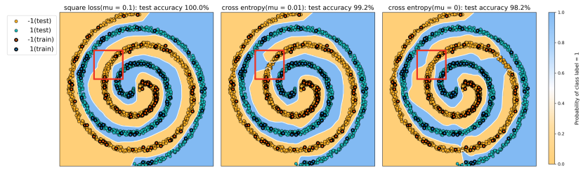
Figure 1: Test misclassification rates and decision boundaries predicted by: SL-ONN + $\ell_{2}$ (Left); CE-ONN + $\ell_{2}$ (Center); CE-ONN (Right) for the separable case.

Non-separable case We consider the conditional probability $\eta(\bm{x})=\sin(\sqrt{2}\pi||\bm{x}||_{2}),\bm{x}\in[-1,1]^{2}$, and the calibration performance of SL-ONN + $\ell_{2}$ and CE-ONN + $\ell_{2}$, where the classifiers are denoted by $\widehat{f}_{l2}$ and $\widehat{f}_{ce}$, respectively. The results are presented in Figure G.8 in the Appendix. The error bar plot of the test calibration error shows that $\widehat{f}_{l2}$ has the smaller mean and standard deviation than $\widehat{f}_{ce}$. It suggests that square loss generally outperforms cross entropy in calibration. The histogram and kernel density estimation of the test calibration errors for one case show that the pointwise calibration errors on the test points of $\widehat{f}_{l2}$ are more concentrated around zero than those of $\widehat{f}_{ce}$. Moreover, despite a comparable misclassification rate with $\widehat{f}_{ce}$, $\widehat{f}_{l2}$ has a smaller calibration error. Figure G.8 demonstrates that SL-ONN + $\ell_{2}$ recovers $\eta$ much better than CE-ONN + $\ell_{2}$.

5.2 Real Data

To make a fair comparison, we adopt popular architectures, ResNet [39] and Wide ResNet [40] and evaluate them on the CIFAR image classification datasets, with only the training loss function changed, from cross-entropy (CE) to square loss with simplex coding (SL). Further, we don’t employ any large scale hyper-parameter tuning and all the parameters are kept as default except for the learning rate (lr) and batch size (bs), where we are choosing from the better of (lr=0.01, bs=32) and (lr=0.1, bs=128). Each experiment setting is replicated 5 times and we report the average performance followed by its standard deviation in the parenthesis. (lr=0.01, bs=32) works better for the most cases except for square loss trained WRN-16-10 on CIFAR-100. More experiment details and additional results can be found in Appendix G.2.

Generalization In both CIFAR-10 and CIFAR-100, the performance of cross-entropy and square loss with simplex coding are quite comparable, as observed in [4]. Cross-entropy tends to perform slightly better for ResNet, especially on CIFAR-100 with an advantage of less than 1%. There is a more significant gap with Wide ResNet where square loss outperforms cross-entropy by more than 1% on both CIFAR-10 and CIFAR-100. The details can be found in Table 1.

Table 1: Test accuracy on CIFAR datasets. Average accuracy larger than 0 but less than 0.1 is denoted as 0^∗ without standard deviation.

Dataset	Network	Loss	Clean acc %	PGD-100 ($l_{\infty}$-strength)			AutoAttack ($l_{\infty}$-strength)
				${2}/{255}$	$4/255$	$8/255$	$2/255$	$4/255$	$8/255$
CIFAR-10	ResNet-18	CE	95.15 (0.11)	8.81 (1.61)	0.65 (0.24)	0	2.74 (0.09)	$0$	0
		SL	95.04 (0.07)	30.53 (0.92)	6.64 (0.67)	0.86 (0.24)	4.10 (0.50)	0∗	0
	WRN-16-10	CE	93.94 (0.16)	1.04 (0.10)	0	0	0.33 (0.06)	0	0
		SL	95.02 (0.11)	37.47 (0.61)	23.16 (1.28)	7.88 (0.72)	5.37 (0.50)	0∗	0
CIFAR-100	ResNet-50	CE	79.82 (0.14)	2.31 (0.07)	0∗	0	0.99 (0.10)	0∗	0
		SL	78.91 (0.14)	13.76 (1.30)	4.63 (1.20)	1.21 (0.80)	3.67 (0.60)	0.16 (0.05)	0
	WRN-16-10	CE	77.89 (0.21)	0.83 (0.07)	0∗	0	0.42 (0.07)	0	0
		SL	79.65 (0.15)	6.48 (0.40)	0.42 (0.04)	0∗	2.73 (0.20)	0∗	0

Adversarial robustness Naturally trained deep classifiers are found to be adversarially vulnerable and adversarial attacks provide a powerful tool to evaluate classification robustness. For our experiment, we consider the black-box Gaussian noise attack, the classic white-box PGD attack [41] and the state-of-the-art AutoAttack [42], with attack strength level 2/255, 4/255, 8/255 in $l_{\infty}$ norm. AutoAttack contains both white-box and black-box attacks and offers a more comprehensive evaluation of adversarial robustness. The Gaussian noises results are presented in Table G.3 in the Appendix. At different noise levels, square loss consistently outperforms cross-entropy, especially for WRN-16-10, with around 2-4% accuracy improvement. More details can be found in Appendix G.2. The PGD and AutoAttack results are reported in Table 1. Even though classifiers trained with square loss is far away from adversarially robust, it consistently gives significantly higher adversarial accuracy. The same margin can be carried over to standard adversarial training as well. Table 2 lists results from standard PGD adversarial training with CE and SL. By substituting cross-entropy loss to square loss, the robust accuracy increased around 3% while maintaining higher clean accuracy.

One thing to notice is that when constructing white-box attacks, square loss will not work well since it doesn’t directly reflect the classification accuracy. More specifically, for a correctly classified image $(\bm{x},y)$, maximizing the square loss may result in linear scaling of the classifier $f(\bm{x})$, which doesn’t change the predicted class (see Appendix G.2 for more discussion). To this end, we consider a special attack for classifiers trained by square loss by maximizing the cosine similarity between $f(\bm{x})$ and $\bm{v}_{y}$. We call this angle attack and also utilize it for the PGD adversarial training paired with square loss in Table 2. In our experiments, this special attack rarely outperforms the standard PGD with cross-entropy and the reported PGD accuracy are from the latter settings. This property of square loss may be an advantage in defending adversarial attacks.

Table 2: Performance on CIFAR-10 dataset for ResNet-18 under standard PGD adversarial training.

CIFAR10	Loss	Acc (%)	PGD steps	Strength($l_{\infty}$)	Autoattack
ResNet-18	CE	86.87	3	8/255	37.08
		84.50	7	8/255	41.88
ResNet-18	SL	87.31	3	8/255	40.46
		84.52	7	8/255	44.76

Model calibration The predicted class probabilities for square loss can be obtained from Equation 4.1. Expected calibration error (ECE) measures the absolute difference between predicted confidence and actual accuracy. Deep classifiers are usually found to be over-confident [43]. Using ResNet as an example, we report the typical reliability diagram in Figure 2. On CIFAR-10 with ResNet-18, the average ECE for cross-entropy is 0.028 (0.002) while that for square loss is 0.0097 (0.001). On CIFAR-100 with ResNet-50, the average ECE for cross-entropy is 0.094 (0.005) while that for square loss is 0.068 (0.005). Square loss results are much more calibrated with significantly smaller ECE.

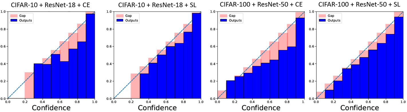
Figure 2: Reliability diagrams of ResNet-18 on CIFAR-10 and ResNet-50 on CIFAR-100. Square loss trained models behave more well-calibrated while cross-entropy trained ones tend to be visibly more over-confident.

6 Conclusions

Classification problems are ubiquitous in deep learning. As a fundamental problem, any progress in classification can potentially benefit numerous relevant tasks. Despite its lack of popularity in practice, square loss has many advantages that can be easily overlooked. Through both theoretical analysis and empirical studies, we identify several ideal properties of using square loss in training neural network classifiers, including provable fast convergence rates, strong robustness, and small calibration error. We encourage readers to try square loss in your own application scenarios.

Appendix A Gradient Descent and Neural Tangent Kernel

Gradient Descent

Since we consider the square loss and $\ell_{2}$ regularization, the optimization problem in Equation 2.2 becomes

$$\min_{\bm{W}}\sum_{i=1}^{n}(f_{\bm{W},\bm{a}}(\bm{x}_{i})-y_{i})^{2}+\mu\left\lVert\bm{W}\right\rVert_{2}^{2}.$$ (A.1)

We consider the GD training of Equation A.1. Let

$$\Phi(\bm{W})=\sum_{i=1}^{n}(f_{\bm{W},\bm{a}}(\bm{x}_{i})-y_{i})^{2}+\mu\left\lVert\bm{W}\right\rVert_{2}^{2}$$

be the objective function in Equation A.1. The gradient of $\Phi$ with respect to $\bm{w}_{r}$ can be written as [30]

$$\frac{\partial\Phi(\bm{W})}{\partial\bm{w}_{r}}=\frac{2}{\sqrt{m}}a_{r}\sum_{i=1}^{n}(u_{i}-y_{i})\mathbb{I}_{r,i}\bm{x}_{i}+2\mu\bm{w}_{r},\quad r\in[m],$$

where $u_{i}=f_{\bm{W},\bm{a}}(\bm{x}_{i})$ and $\mathbb{I}_{r,i}=\mathbb{I}\{\bm{w}_{r}^{\top}\bm{x}_{i}\geq 0\}$. Then the GD update rule is

$$\bm{w}_{r}(k+1)=\bm{w}_{r}(k)-\zeta\frac{\partial\Phi(\bm{W})}{\partial\bm{w}_{r}}\biggm{|}_{\bm{W}=\bm{W}(k)},$$

where $\bm{W}(k)$ is the weight matrix at iteration $k$, and $\zeta$ is the learning rate. Define $\mathbb{I}_{r,i}(k)=\mathbb{I}\{\bm{w}_{r}(k)^{\top}\bm{x}_{i}\geq 0\}$, $\bm{Z}(k)\in\mathbb{R}^{md\times n}$ as

$$\bm{Z}(k)=\frac{1}{\sqrt{m}}\begin{pmatrix}a_{1}\mathbb{I}_{1,1}(k)\bm{x}_{1}&\dots&a_{1}\mathbb{I}_{1,n}(k)\bm{x}_{n}\\ \vdots&dots&\vdots\\ a_{m}\mathbb{I}_{m,1}(k)\bm{x}_{1}&\dots&a_{m}\mathbb{I}_{m,n}(k)\bm{x}_{n}\end{pmatrix},$$

$\bm{H}(k)=\bm{Z}(k)^{\top}\bm{Z}(k)$, and $\bm{u}(k)=(\bm{u}_{1}(k),...,\bm{u}_{n}(k))^{\top}$ with $\bm{u}_{i}(k)=f_{\bm{W}(k),\bm{a}}(\bm{x}_{i})$. Then the GD update rule with respect to $\bm{W}$ can be written as

$${\rm vec}(\bm{W}(k+1))= {\rm vec}(\bm{W}(k))-2\zeta\big{(}\bm{Z}(k)(\bm{u}(k)-\bm{y})+\mu{\rm vec}(\bm{W}(k))\big{)},$$ (A.2)

where $\mathrm{vec}(\bm{W})=(\bm{w}_{1}^{\top},\cdots,\bm{w}_{m}^{\top})^{\top}\in\mathbb{R}^{md\times 1}$ is the vectorized weight matrix and $\bm{y}=(y_{1},...,y_{n})^{\top}$.

Neural Tangent Kernel (NTK)

It has been shown that the following NTK

$$h(\bm{s},\bm{t})= \mathbb{E}_{\bm{w}\sim N(0,\bm{I}_{d})}\left(\bm{s}^{\top}\bm{t}\ \mathbb{I}\{\bm{w}^{\top}\bm{s}\geq 0,\bm{w}^{\top}\bm{t}\geq 0\}\right)=\frac{\bm{s}^{\top}\bm{t}(\pi-\arccos(\bm{s}^{\top}\bm{t}))}{2\pi}$$ (A.3)

plays an important role in the study of one-hidden-layer ReLU neural networks, where $\bm{s},\bm{t}$ are $d$-dimensional vectors [44, 32]. Since $h$ is positive definite on the unit sphere $\mathbb{S}^{d-1}$ [31], by Mercer’s theorem, it possesses a Mercer decomposition as $h(\bm{s},\bm{t})=\sum_{j=0}^{\infty}\lambda_{j}\varphi_{j}(\bm{s})\varphi_{j}(\bm{t}),$ where $\lambda_{1}\geq\lambda_{2}\geq...\geq 0$ are the eigenvalues, and $\{\varphi_{j}\}_{j=1}^{\infty}$ is an orthonormal basis. The asymptotic behavior of the eigenvalues is described in the following lemma.

Lemma A.1 (Lemma 3.1 of Hu et al. [32]).

Let $\lambda_{j}$ be the eigenvalues of NTK $h$ defined above. Then we have $\lambda_{j}\asymp j^{-\frac{d}{d-1}}$.

Let $\mathcal{N}$ denote the reproducing kernel Hilbert space (RKHS) generated by $h$ on $\mathbb{S}^{d-1}$, equipped with norm $\left\lVert\cdot\right\rVert_{\mathcal{N}}$. As a corollary of Lemma A.1, it can be shown that the ($L_{\infty}$) entropy number of a unit ball in $\mathcal{N}$, denoted by $\mathcal{N}(1)$, can be controlled. The relationship between the eigenvalues and entropy numbers has been well studied; see [45].

Lemma A.2.

The entropy number of $\mathcal{N}(1)$, denoted by $H(\mathcal{N}(1),\delta,\left\lVert\cdot\right\rVert_{L_{\infty}})$, is bounded by $H(\mathcal{N}(1),\delta,\left\lVert\cdot\right\rVert_{L_{\infty}})\lesssim\delta^{-2(d-1)/d}$.

There are extensive works studying the generalization error bounds under NTK regime. For regression, Nitanda and Suzuki [46], Hu et al. [32] show the optimal convergence rates when using overparametrized one-hidden-layer neural networks, where the square loss is used. Arora et al. [30] provides generalization error bounds and provable learning scenarios for noiseless data. In the NTK regime, the neural network as a regressor is linked with the nonparametric regression via NTK. There are also other works studying the generalization performance of the neural network as a nonparametric regressor, out of the NTK regime; see [47, 48]. For classification, most of the existing results are established based on the separable data; see [22, 24, 49] and references therein. In particular, Hu et al. [23] consider classification with noisy labels (labels are randomly flipped) and propose to use the square loss with $\ell_{2}$ regularization. Besides the generalization error bounds, another important research direction is to bridge the gap between NTK and finite-width overparametrized neural networks via GD training; see [44, 30, 50, 32], among others.

Appendix B Overview of Reproducing Kernel Hilbert Space

We provide here a brief overview of reproducing kernel Hilbert space (RKHS).

Definition B.1 (Positive Definite Kernel).

A function $k:\Omega\times\Omega\mapsto\mathbb{R}$ is said to be a positive definite kernel, if $k(\bm{x},\widetilde{\bm{x}})=k(\widetilde{\bm{x}},\bm{x})$ for all $\bm{x},\widetilde{\bm{x}}\in\Omega$, and

$$\sum_{i=1}^{n}\sum_{j=1}^{n}\beta_{i}\beta_{j}k(\bm{x}_{i},\bm{x}_{j})>0,$$

for all $n\in\mathbb{N}$, $\beta_{1},\ldots,\beta_{n}\in\mathbb{R}$ such that at least one $\beta_{j}\neq 0$, and $\bm{x}_{1},\ldots,\bm{x}_{n}\in\Omega$.

For a positive definite kernel $k$, define a linear space

$$\mathcal{N}^{0}_{k}:=\left\{\sum_{i=1}^{n}\beta_{i}k(\cdot,\bm{x}_{i}):n\in\mathbb{N},\;\beta_{1},\ldots,\beta_{n}\in\mathbb{R},\;\bm{x}_{1},\ldots,\bm{x}_{n}\in\Omega\right\},$$

and equip this space with an inner product $\langle\cdot,\cdot\rangle_{\mathcal{N}^{0}_{k}}$ by

$$\left\langle\sum_{i=1}^{n}\beta_{i}k(\cdot,\bm{x}_{i}),\sum_{j=1}^{\widetilde{n}}\widetilde{\beta}_{j}k(\cdot,\widetilde{\bm{x}}_{i})\right\rangle_{\mathcal{N}^{0}_{k}}:=\sum_{i=1}^{n}\sum_{j=1}^{\widetilde{n}}\beta_{i}\widetilde{\beta}_{j}k(\bm{x}_{i},\widetilde{\bm{x}}_{j}).$$

The norm of $g\in\mathcal{N}^{0}_{k}$ is defined by $\left\lVert g\right\rVert_{\mathcal{N}^{0}_{k}}^{2}:=\langle g,g\rangle_{\mathcal{N}^{0}_{k}}$. Then the RKHS induced by $k$, denoted by $\mathcal{N}_{k}(\Omega)$, is defined as the closure of $\mathcal{N}^{0}_{k}(\Omega)$ with respect to the norm $\left\lVert\cdot\right\rVert_{\mathcal{N}^{0}_{k}(\Omega)}$.

For a subset $\Omega_{0}\subset\Omega$, define the restriction of $\mathcal{N}_{k}$ on $\Omega_{0}$ as

$$\mathcal{N}_{k}(\Omega_{0}):=\left\{g:\Omega_{0}\mapsto\mathbb{R}:g=h|_{\Omega_{0}}\mbox{ for some }h\in\mathcal{N}_{k}\right\},$$

where $g=h|_{\Omega_{0}}$ means $g(\bm{x})=h(\bm{x})$ for all $\bm{x}\in\Omega_{0}$. We equip $\mathcal{N}_{k}(\Omega_{0})$ with norm

$$\left\lVert g\right\rVert_{\mathcal{N}_{k}(\Omega_{0})}:=\inf_{\{h\in\mathcal{N}_{k}:h|_{\Omega_{0}}=g\}}\left\lVert h\right\rVert_{\mathcal{N}_{k}}.$$

Then, $\mathcal{N}_{k}(\Omega_{0})$ is a RKHS with norm $\left\lVert\cdot\right\rVert_{\mathcal{N}_{k}(\Omega_{0})}$ (see Aronszajn 51, page 351).

Appendix C Simplex Coordinates

In simplex label coding, the one-hot labels are replaced by the simplex vertices of a $(K-1)$-simplex. The vertices of a regular $(K-1)$-simplex centered on the origin can be written as:

$$\bm{v}_{0}=\frac{1}{{\sqrt{2K}}}\cdot(1,\dots,1)$$

and for $1\leq i\leq K-1$,

$$\bm{v}_{i}=\frac{1}{\sqrt{2}}\bm{e}_{i}-\frac{1}{(K-1){\sqrt{2}}}\left(1+\frac{1}{\sqrt{K}}\right)\cdot(1,\dots,1).$$

The pairwise angle between vertices is $\arccos(-1/(K-1))$ and as $K\to\infty$, the angle converges to $90^{\circ}$.

The vertices of a $(K-1)$-simplex can be viewed as maximally separated $K$ points on a sphere. In theory, the radius of the sphere doesn’t matter but in practice, we recommend scaling it for larger number of classes, e.g., radius = $K$ for $K$-class classification. We find that such scaling empirically outperforms the default radius 1 in our experiments. More details can be found in Appendix G.2.

Appendix D Assumptions

In this work, we impose the following assumptions. In the rest of the Appendix, we use ${\rm poly}(t_{1},t_{2},\ldots)$ to denote some polynomial function with arguments $t_{1},t_{2},\ldots$.

Assumption D.1.

Let $\lambda_{\min}(\bm{H}^{\infty})$ be the minimum eigenvalue of the symmetric matrix $\bm{H}^{\infty}$, where $\bm{H}^{\infty}=\left(h(\bm{x}_{i},\bm{x}_{j})\right)_{n\times n}$ ($\bm{H}^{\infty}$ is usually called the NTK matrix). Let $\lambda_{0}$ be the largest number such that with probability at least $1-\delta_{n}$, $\lambda_{\min}(\bm{H}^{\infty})\geq\lambda_{0}$, and $\delta_{n}\rightarrow 0$ as $n$ goes to infinity. For sufficiently large $n$, the regularization parameter $\mu\asymp n^{\frac{d-1}{2d-1}}$, the learning rate $\zeta=o(n^{-\frac{3d-1}{2d-1}})$, the variance of initialization $\xi^{2}=O(1)$, the number of nodes in the hidden layer $m\geq\xi^{-2}{\rm ploy}(n,\lambda_{0}^{-1})$, and the iteration number $k$ satisfies $\log\left({\rm ploy}_{1}(n,\xi,1/\lambda_{0})\right)\lesssim\zeta\mu k\lesssim\log\left({\rm ploy}_{2}(\xi,1/n,\sqrt{m})\right).$

Assumption D.2.

The conditional probability in the non-separable case satisfies $\eta\in\mathcal{N}$.

Assumption D.3.

The solution to Equation 2.2 satisfies $\left\lVert f_{\bm{W}(k),\bm{a}}\right\rVert_{\mathcal{N}}\leq C$, where $C$ is a constant not depending on $n$.

Remark 5.

Assumption D.3 can be replaced by a stronger assumption, that is, $f_{\bm{W}(k),\bm{a}}$ has a bounded Lipschitz constant, and the constant does not depend on $n$.

Assumption D.4.

The probability density function of the marginal distribution $P_{X}$, denoted by $p({\bm{x}})$, is continuous on $\Omega$, and there exists a positive constant $c_{0}$ such that

$$p({\bm{x}})\leq c_{0},\forall{\bm{x}}\in\Omega.$$

Assumption D.5.

The probability density function of the marginal distribution $p({\bm{x}})$ is continuous on $\Omega$, and there exist positive constants $c_{1}\leq c_{2}$ such that

$$c_{1}\leq p({\bm{x}})\leq c_{2},\forall{\bm{x}}\in\Omega.$$

Assumption D.1 is related to the neural network and GD training, where similar settings have been adopted by Arora et al. [30], Hu et al. [32]. From the results in [30, 32], the width of the neural network depends on the minimum eigenvalue of the NTK matrix $\lambda_{\min}(\bm{H}^{\infty})$, where a smaller $\lambda_{\min}(\bm{H}^{\infty})$ leads to a wider neural network. Therefore, it is desired that $\lambda_{0}$ is as large as possible. However, the consistency requires that the probability is tending to one; thus, we require $\delta_{n}\rightarrow 0$ as $n\rightarrow\infty$. As $n$ becomes larger, with probability tending to one, the distance of the two nearest points in $n$ input points converges to zero, thus making $\bm{H}^{\infty}$ close to a degenerate matrix, and the minimum eigenvalue of $\bm{H}^{\infty}$ converges to zero. Therefore, inevitably, $\lambda_{0}\rightarrow 0$ (but $\lambda_{\min}(\bm{H}^{\infty})$ is strictly larger than 0 for all $n$ with probability one). The requirements of the regularization parameter, the learning rate, the variance of initialization, the number of nodes in the hidden layer and the iteration number are all the same as those in [32].

Assumption D.2 imposes conditions on the underlying true conditional probability in the non-separable case. This assumption basically requires that the conditional probability is within the function class generated by the GD-trained neural networks we consider (thus can be calibrated). Given that the neural networks are highly flexible, we believe that most of the functions are within the function class generated by the neural networks. As a simple example, any Lipschitz functions are within this function class.

Assumption D.3 requires that the solution to Equation 2.2 is well-behaved, i.e., the solution is within a ball in $\mathcal{N}$ with a certain radius. Roughly speaking, Assumption D.3 requires that the complexity of the neural network estimator generated by the GD training is controlled. Since the step size is relatively small and the iteration number is not large (only $\log({\rm poly}(n,\xi,,\lambda_{0}^{-1})$), we believe it is a mild assumption.

Assumption D.4 only requires the probability to be upper bounded from infinity, while Assumption D.5 requires the probability to be upper bounded from infinity and lower bounded away from zero on the support $\Omega$. They are standard assumptions used in the classical analysis of classification in statistics; see Audibert and Tsybakov [17], Kohler and Krzyzak [18] for example. Clearly, uniform distribution satisfies Assumptions D.4 and D.5. In Audibert and Tsybakov [17], Assumption D.4 is called mild density assumption and Assumption D.5 is called strong density assumption.

Appendix E Proofs of Main Results

This section includes the proofs of main results in the paper.

E.1 Proof of Theorem 3.1

We first introduce some lemmas that are used in the proof of Theorem 3.1.

Let $l_{1}(y_{i},f(\bm{x}_{i}))=(1-y_{i}f(\bm{x}_{i}))^{2}=(y_{i}-f(\bm{x}_{i}))^{2}$ be the square loss on a training point $(\bm{x}_{i},y_{i})$, the $l_{1}$-risk of $f$ be $\mathcal{R}_{l_{1}}(f)=\mathbb{E}_{X,Y\sim P}l_{1}(Y,f(X))$, and $\mathcal{R}_{l_{1}}=\min_{f\in\mathcal{N}}\mathbb{E}_{X,Y\sim P}l_{1}(Y,f(X))$. Let $L_{1}(f,\bm{x},y)=\mu\left\lVert f\right\rVert_{\mathcal{N}}^{2}+l_{1}(y,f(\bm{x}))$ and the $L_{1}$-risk of $f$ be $\mathcal{R}_{L_{1}}(f)=\mathbb{E}_{X,Y\sim P}L_{1}(f,X,Y)$. Let $f_{n}=\mathop{\mathrm{argmin}}_{f\in\mathcal{N}}\mathcal{R}_{L_{1}}(f)$.

Lemma E.1 is (a weaker version of) Theorem 5.6 of Steinwart et al. [19], which provides a bound on the deviation between the empirical minimizer and true minimizer. Lemma E.2 is used to verify that one of the conditions of Lemma E.1 is fulfilled. Lemma E.3 shows that under certain conditions, the solution to

$$\min_{f\in\mathcal{N}}\frac{1}{n}\sum_{i=1}^{n}(y_{i}-f(\bm{x}_{i}))^{2}+\frac{\mu}{n}\left\lVert f\right\rVert_{\mathcal{N}}^{2}$$ (E.1)

is closely related to the estimator given by the overparameterized neural networks $f_{\bm{W}(k),\bm{a}}$. Lemma E.3 can be obtained by merely repeating the proof of Theorem 5.2 of Hu et al. [32], since we require that the probability density function $p({\bm{x}})$ of $P_{X}$ is upper bounded by a positive constant by Assumption D.4. Therefore, the only difference is that we replace $\left\lVert\cdot\right\rVert_{2}$ (which corresponds to the uniform distribution) to the $L_{2}$ norm corresponding to the probability measure $P_{X}$; thus the proof is omitted. Note also that the second statement of Lemma E.3 corresponds to the noiseless case.

Lemma E.1.

Let $Z=\Omega\times\{-1,1\}$. Let $\mathcal{F}$ be a convex set of bounded measurable functions from $Z$ to $\mathbb{R}$ and let $L:\mathcal{F}\times Z\rightarrow[0,\infty)$ be a convex and continuous loss function. For a probability measure $P$ on $Z$, define

$$\mathcal{G}:=\{L\circ f-L\circ{f}_{P,\mathcal{F}}:f\in\mathcal{F}\},$$

where ${f}_{P,\mathcal{F}}$ is a minimizer of $\mathbb{E}_{Z\sim P}L(f,Z)$. Suppose that there are constants $c\geq 0$, $0<\alpha\leq 1$, $\delta\leq 0$ and $B>0$ such that $\mathbb{E}_{Z\sim P}{g}^{2}\leq c(\mathbb{E}_{Z\sim P}g)^{\alpha}+\delta$ and $||g||_{\infty}\leq B$ for all $g\in\mathcal{G}$. Furthermore, assume that $\mathcal{G}$ is separable with respect to $\left\lVert\cdot\right\rVert_{\infty}$ and that there are constants $a\geq 1$ and $0<\alpha<2$ with

$$\sup_{T\in Z^{n}}H(B^{-1}\mathcal{G},\epsilon,\left\lVert\cdot\right\rVert_{L_{2}(T)})\leq a\epsilon^{-\beta}$$ (E.2)

for all $\epsilon>0$, where $H(B^{-1}\mathcal{G},\epsilon,\left\lVert\cdot\right\rVert_{L_{2}(T)})$ is the entropy number of the set $B^{-1}\mathcal{G}$, and $\left\lVert f\right\rVert_{L_{2}(T)}^{2}=\frac{1}{n}\sum_{i=1}^{n}f({\bm{x}}_{i},y_{i})^{2}$ is the empirical norm. Then there exists a constant $c_{\beta}>0$ depending only on $\beta$ such that for all $n\geq 1$ and all $t\geq 1$ we have

$$\mathbb{P}(T\in Z^{n}:\mathcal{R}_{L,P}(f_{T,\mathcal{F}})>\mathcal{R}_{L,P}(f_{P,\mathcal{F}})+c_{\beta}\varepsilon(n,a,B,c,\delta,t))\leq e^{-t},$$

where

$$\varepsilon(n,a,B,c,\delta,t)$$

$$= B^{2\beta/(4-2\alpha+\alpha p)}c^{(2-\beta)/(4-2\alpha+\alpha\beta)}\left(\frac{a}{n}\right)^{2/(4-2\alpha+\alpha\beta)}+B^{\beta/2}\delta^{(2-\beta)/4}\left(\frac{a}{n}\right)^{1/2}$$

$$+B\left(\frac{a}{n}\right)^{2/(2+\beta)}+\sqrt{\frac{\delta t}{n}}+\left(\frac{ct}{n}\right)^{1/(2-\alpha)}+\frac{Bt}{n},$$ (E.3)

and $f_{T,\mathcal{F}}$ is the minimizer with respect to the empirical measure.

Lemma E.2.

Assume the conditions of Theorem 3.1 hold. Define $C:=8||(2\eta-1)^{-1}||_{\kappa,\infty}+32$, where $\left\lVert\cdot\right\rVert_{\kappa,\infty}$ is the norm of Lorentz space $L_{\kappa,\infty}$ [52]. Let $\mu>0$ and $0<\gamma\leq n^{1/2}\mu^{-1/2}$, then for all $f\in\gamma\mathcal{N}(1)$ we have

$$\mathbb{E}_{X,Y\sim P}(L_{1}\circ f-L_{1}\circ f_{n})^{2}\leq C(K\gamma+1)^{2}(\mathbb{E}_{X,Y\sim P}(L_{1}\circ f-L_{1}\circ f_{n}))+2C(K\gamma+1)^{2}a(\mu),$$

where $a(\mu)$ is the approximation error function given by

$$a(\mu)=\inf_{f\in\mathcal{N}}(n^{-1}\mu||f||_{\mathcal{N}}^{2}+\mathcal{R}_{l_{1}}(f)-\mathcal{R}_{l_{1}}).$$

Lemma E.3.

Suppose Assumptions D.1 and D.4 hold. Then we have

$$\mathbb{E}_{X\sim P_{X}}(f_{\bm{W}(k),\bm{a}}(X)-\widehat{f}(X))^{2}=O_{\mathbb{P}}(n^{-\frac{d}{2d-1}}),$$

where $\widehat{f}$ is the solution to Equation E.1. Furthermore, if there exists a function $f\in\mathcal{N}$ that does not depend on $n$ and $f({\bm{x}}_{i})=y_{i}$ for all $i=1,...,n$, then we can set $\mu=o(1)$ and obtain

$$\mathbb{E}_{X\sim P_{X}}(f_{\bm{W}(k),\bm{a}}(X)-\widehat{f}(X))^{2}=o_{\mathbb{P}}(1).$$

Remark 6.

According to the proof in [32], the probability in $o_{\mathbb{P}}(1)$ of Lemma E.3 only relates to the width of the one-hidden-layer neural network, which can be arbitrarily small by enlarging the neural network’s width.

Now we are ready to prove Theorem 3.1. Let $L=L_{1}$ in Lemma E.1, which is clearly continuous. Let $\widehat{f}$ be the solution to Equation E.1. The key idea in this proof is using $\widehat{f}$ to bridge two functions $2\eta-1$ and $f_{\bm{W}(k),\bm{a}}$.

Since $\widehat{f}$ is the solution to Equation E.1, it can be seen that

$$\frac{1}{n}\sum_{i=1}^{n}(y_{i}-\widehat{f}({\bm{x}}_{i}))^{2}+\frac{\mu}{n}\left\lVert\widehat{f}\right\rVert_{\mathcal{N}}^{2}\leq \frac{1}{n}\sum_{i=1}^{n}(y_{i}-(2\eta({\bm{x}}_{i})-1))^{2}+\frac{\mu}{n}\left\lVert 2\eta({\bm{x}}_{i})-1\right\rVert_{\mathcal{N}}^{2}$$

$$\leq \frac{2}{n}\sum_{i=1}^{n}(y_{i}^{2}+(2\eta({\bm{x}}_{i})-1)^{2})+\frac{\mu}{n}\left\lVert 2\eta({\bm{x}}_{i})-1\right\rVert_{\mathcal{N}}^{2}$$

$$\leq C_{1},$$ (E.4)

where the second inequality is by the Cauchy-Schwarz inequality, and the third inequality is because $y_{i}^{2}=1$ and $\eta({\bm{x}})$ is bounded.

The reproducing property implies that

$$\widehat{f}({\bm{x}})=\langle\widehat{f},h({\bm{x}},\cdot)\rangle_{\mathcal{N}}\leq\left\lVert\widehat{f}\right\rVert_{\mathcal{N}}\left\lVert h({\bm{x}},\cdot)\right\rVert_{\mathcal{N}}=\left\lVert\widehat{f}\right\rVert_{\mathcal{N}}\sqrt{h({\bm{x}},{\bm{x}})},\forall{\bm{x}}\in\Omega,$$

which yields

$$\left\lVert\widehat{f}\right\rVert_{L_{\infty}}\leq C_{2}\left\lVert\widehat{f}\right\rVert_{\mathcal{N}}.$$

Together with Equation E.1, we obtain

$$\left\lVert\widehat{f}\right\rVert_{L_{\infty}}\leq C_{3}\left\lVert\widehat{f}\right\rVert_{\mathcal{N}}\leq C_{4}(\mu/n)^{-1/2}.$$ (E.5)

Thus, we can take $B=C_{4}(\mu/n)^{-1/2}$ in Lemma E.1. The entropy condition can be verified via Lemma A.2, which allows us to take $\beta=2(d-1)/d$. Equation E.5, together with Lemma E.2, also suggests that we can take $c=C(KB+1)^{2}$, $\alpha=1$, and $\delta=2C(KB+1)^{2}a(\mu)$.

Next, we provide an upper bound on $a(\mu)$. The definition of $a(\mu)$ implies

$$a(\mu)= n^{-1}\mu\left\lVert f_{n}\right\rVert_{\mathcal{N}}^{2}+R_{l_{1}}(f_{n})-R_{l_{1}}$$

$$= n^{-1}\mu\left\lVert f_{n}\right\rVert_{\mathcal{N}}^{2}+\mathbb{E}_{X\sim P_{X}}(2\eta(X)-1-f_{n}(X))^{2}$$

$$\leq n^{-1}\mu\left\lVert 2\eta-1\right\rVert_{\mathcal{N}}^{2},$$ (E.6)

where we use the relationship $\mathcal{R}_{l_{1},P}(f)-\mathcal{R}_{l_{1},P}=\mathbb{E}_{X\sim P_{X}}(2\eta(X)-1-f(X))^{2}$.

Plugging all the terms into Equation E.1, together with Lemma E.1, yields that

$$\mathcal{R}_{L_{1},P}(\widehat{f})=\mathcal{R}_{L_{1},P}(f_{n})+O_{\mathbb{P}}(\varepsilon(n,a,B,c,\delta)),$$ (E.7)

where

$$\varepsilon(n,a,B,c,\delta)= B^{\frac{4}{2+\beta}}n^{-\frac{2}{2+\beta}}+B(\mu/n)^{\frac{2-\beta}{4}}n^{-\frac{1}{2}}\left\lVert 2\eta-1\right\rVert_{\mathcal{N}}^{\frac{2-\beta}{2}}+B^{2}n^{-1}$$

$$= B^{\frac{4d}{4d-2}}n^{-\frac{2d}{4d-2}}+B\mu^{\frac{1}{2d}}n^{-\frac{1}{2}-\frac{1}{2d}}\left\lVert 2\eta-1\right\rVert_{\mathcal{N}}^{\frac{1}{d}}+B^{2}n^{-1}.$$ (E.8)

Since $\mathcal{R}_{l_{1},P}(f)-\mathcal{R}_{l_{1},P}=\mathbb{E}_{X\sim P_{X}}(2\eta(X)-1-f(X))^{2}$, we subtract $\mathcal{R}_{l_{1},P}$ on both sides of Equation E.7 and get

$$\mathbb{E}_{X\sim P_{X}}(2\eta(X)-1-\widehat{f}(X))^{2}+n^{-1}\mu\left\lVert\widehat{f}\right\rVert_{\mathcal{N}}^{2}$$

$$= \mathbb{E}_{X\sim P_{X}}(2\eta(X)-1-f_{n}(X))^{2}+n^{-1}\mu\left\lVert f_{n}\right\rVert_{\mathcal{N}}^{2}+O_{\mathbb{P}}(\varepsilon(n,a,B,c,\delta))$$

$$= O_{\mathbb{P}}(n^{-1}\mu\left\lVert 2\eta-1\right\rVert_{\mathcal{N}}^{2}+\varepsilon(n,a,B,c,\delta)),$$ (E.9)

where the last equality (with big $O$ notation) is by Equation E.1. Combining Equation E.1 and Equation E.5 implies

$$\left\lVert\widehat{f}\right\rVert_{L_{\infty}}^{2}\leq C_{3}^{2}\left\lVert\widehat{f}\right\rVert_{\mathcal{N}}^{2}=O_{\mathbb{P}}(1+n\mu^{-1}\varepsilon(n,a,B,c,\delta)).$$

In the following, we will show that by taking $\mu\asymp n^{\frac{d-1}{2d-1}}$,

$$\mathbb{E}_{X\sim P_{X}}(2\eta(X)-1-\widehat{f}(X))^{2}+n^{-1}\mu\left\lVert\widehat{f}\right\rVert_{\mathcal{N}}^{2}=O_{\mathbb{P}}(n^{-\frac{d}{2d-1}}\max(1,\left\lVert 2\eta-1\right\rVert_{\mathcal{N}}^{\frac{2}{d}}))=O_{\mathbb{P}}(n^{-\frac{d}{2d-1}}).$$ (E.10)

If $n\mu^{-1}\varepsilon(n,a,B,c,\delta)\lesssim 1$, then $\varepsilon(n,a,B,c,\delta)\lesssim\mu/n$, and Equation E.10 holds. Otherwise, we can replace $B^{2}$ by its upper bound $O_{\mathbb{P}}(n\mu^{-1}\varepsilon(n,a,B,c,\delta))$ in Equation E.1 and obtain that

$$\varepsilon=O_{\mathbb{P}}(\varepsilon^{\frac{d}{2d-1}}\mu^{-\frac{d}{2d-1}}+\varepsilon^{\frac{1}{2}}\mu^{-\frac{d-1}{2d}}n^{-\frac{1}{2d}}\left\lVert 2\eta-1\right\rVert_{\mathcal{N}}^{\frac{1}{d}}),$$

where we set $\varepsilon=\varepsilon(n,a,B,c,\delta)$ for notational simplicity. Let us hereby denote $I_{1}=\varepsilon^{\frac{d}{2d-1}}\mu^{-\frac{d}{2d-1}}$ and $I_{2}=\varepsilon^{\frac{1}{2}}\mu^{-\frac{d-1}{2d}}n^{-\frac{1}{2d}}\left\lVert 2\eta-1\right\rVert_{\mathcal{N}}^{\frac{1}{d}}$, and consider the following two cases.

Case 1: $I_{1}\geq I_{2}$, then we have

$$\varepsilon=O_{\mathbb{P}}(\varepsilon^{\frac{d}{2d-1}}\mu^{-\frac{d}{2d-1}}).$$

Solving this equality leads to

$$\varepsilon=O_{\mathbb{P}}(\mu^{-\frac{d}{d-1}}).$$ (E.11)

Plugging Equation E.11 into Equation E.1 and minimize the right-hand side of Equation E.1 with respect to $\mu$ gives us $\mu\asymp n^{\frac{d-1}{2d-1}}$; thus Equation E.10 holds.

Case 2: $I_{1}<I_{2}$, then we have

$$\varepsilon=O_{\mathbb{P}}(\varepsilon^{\frac{1}{2}}\mu^{-\frac{d-1}{2d}}n^{-\frac{1}{2d}}\left\lVert 2\eta-1\right\rVert_{\mathcal{N}}^{\frac{1}{d}}),$$

which leads to

$$\varepsilon=O_{\mathbb{P}}(\mu^{-\frac{d-1}{d}}n^{-\frac{1}{d}}\left\lVert 2\eta-1\right\rVert_{\mathcal{N}}^{\frac{2}{d}}).$$ (E.12)

Similarly, we plug Equation E.12 into Equation E.1 and minimize the right-hand side of Equation E.1 with respect to $\mu$ and obtain $\mu\asymp n^{\frac{d-1}{2d-1}}$, which also leads to Equation E.10.

Now we can obtain an upper bound on the excess risk. For the notation simplicity, let $f=f_{\bm{W}(k),\bm{a}}$. The excess risk can be bounded by

$$L(f)-L^{*}\leq \mathbb{E}_{X\sim P_{X}}\mathbb{I}\{(2\eta(X)-1)f(X)\leq 0,|\eta(X)-0.5|<\delta\}|2\eta(X)-1|$$

$$+\mathbb{E}_{X\sim P_{X}}\mathbb{I}\{(2\eta(X)-1)f(X)\leq 0,|\eta(X)-0.5|\geq\delta\}|2\eta(X)-1|.$$ (E.13)

The first term can be bounded via Tsybakov’s noise condition as

$$\mathbb{E}_{X\sim P_{X}}\mathbb{I}\{(2\eta(X)-1)f(X)\leq 0,|\eta(X)-0.5|<\delta\}|2\eta(X)-1|\leq 2\delta\mathbb{E}[\mathbb{I}\{|\eta(X)-0.5|<\delta\}]$$

$$= 2\delta\mathbb{P}(|\eta(X)-0.5|<\delta)\leq 2C\delta^{\kappa+1}.$$ (E.14)

It remains to bound the second term in Equation E.1. If $p(\bm{x})$ is continuous, then by the fact that $|2\eta(X)-1|\leq|2\eta(X)-1-f(X)|$ if $(2\eta(X)-1)f(X)\leq 0$, we have

$$\mathbb{E}_{X\sim P_{X}}\mathbb{I}\{(2\eta(X)-1)f(X)\leq 0,|\eta(X)-0.5|\geq\delta\}|2\eta(X)-1|$$

$$\leq 2\delta^{-1}\mathbb{E}_{X\sim P_{X}}\mathbb{I}\{(2\eta(X)-1)f(X)\leq 0,|\eta(X)-0.5|\geq\delta\}|2\eta(X)-1|^{2}$$

$$\leq 2\delta^{-1}\mathbb{E}_{X\sim P_{X}}\mathbb{I}\{|\eta(X)-0.5|\geq\delta\}(2\eta(X)-1-f(X))^{2}$$

$$\leq 2\delta^{-1}\mathbb{E}_{X\sim P_{X}}(2\eta(X)-1-f(X))^{2}$$

$$\leq 4\delta^{-1}\mathbb{E}_{X\sim P_{X}}(2\eta(X)-1-\widehat{f}(X))^{2}+4\delta^{-1}\mathbb{E}_{X\sim P_{X}}(f(X)-\widehat{f}(X))^{2}$$

$$= O_{\mathbb{P}}(\delta^{-1}n^{-\frac{d}{2d-1}}),$$ (E.15)

where the fourth inequality is by the Cauchy-Schwarz inequality, and the last equality (with big $O$ notation) is by Equation E.10 and Lemma E.3. Taking $\delta=n^{-\frac{d}{(2d-1)(\kappa+2)}}$, and plugging Equation E.1 and Equation E.1 into Equation E.1 leads to

$$L(f)=L^{\star}+O_{\mathbb{P}}(n^{-\frac{d(\kappa+1)}{(2d-1)(\kappa+2)}}).$$

This finishes the proof.

E.2 Proof of Theorem 3.2

We first present a lemma.

Lemma E.4.

Suppose two sets are separable with a positive margin $\gamma>0$. Then there exists a function $f_{T}$ satisfying

$$f_{T}({\bm{x}})=1,\forall{\bm{x}}\in\Omega_{1},\quad f_{T}({\bm{x}})=-1,\forall{\bm{x}}\in\Omega_{2}.$$

Proof of Theorem 3.2. By the equivalence of the RKHS generated by the Laplace kernel and $\mathcal{N}$ [35, 36], it can be shown that $\mathcal{N}$ can be embedded into the Sobolev space $W_{2}^{\nu}$ for some $\nu>d/2$. Consider the Hölder space $C^{0,\alpha}_{b}$ for $0<\alpha\leq 1$ equipped with the norm

$$\left\lVert f\right\rVert_{C_{b}^{0,\alpha}}:=\sup_{{\bm{x}},{\bm{x}}^{\prime}\in\Omega,{\bm{x}}\neq{\bm{x}}^{\prime}}\frac{|f({\bm{x}})-f({\bm{x}}^{\prime})|}{\left\lVert{\bm{x}}-{\bm{x}}^{\prime}\right\rVert_{2}^{\alpha}}.$$ (E.16)

By the Sobolev embedding theorem, we have the embedding relationship

$$\left\lVert f\right\rVert_{C_{b}^{0,\tau}}\leq C_{1}\left\lVert f\right\rVert_{W^{\nu}_{2}}\leq C_{2}\left\lVert f\right\rVert_{\mathcal{N}}$$ (E.17)

for all $f\in\mathcal{N}$, where $\tau=\min(\nu-d/2,1)$.

Without loss of generality, let us consider ${\bm{x}}\in\Omega_{1}$. The case of ${\bm{x}}\in\Omega_{2}$ can be proved similarly. For any ${\bm{x}}\in\Omega_{1}$, take ${\bm{x}}^{\prime}=\mathop{\mathrm{argmin}}_{{\bm{x}}_{i}}\left\lVert{\bm{x}}_{i}-{\bm{x}}\right\rVert_{2}$. Thus, the definition of the Hölder space and Equation E.17 imply

$$|f_{\bm{W}(k),\bm{a}}({\bm{x}})-f_{\bm{W}(k),\bm{a}}({\bm{x}}^{\prime})|\leq C_{2}\left\lVert f_{\bm{W}(k),\bm{a}}\right\rVert_{\mathcal{N}}\left\lVert{\bm{x}}^{\prime}-{\bm{x}}\right\rVert_{2}^{\tau}\leq C_{3}\left\lVert{\bm{x}}^{\prime}-{\bm{x}}\right\rVert_{2}^{\tau},$$ (E.18)

where the last inequality is by Assumption D.3.

Let $\widehat{f}$ be the solution to Equation E.1, and let $\widehat{f}_{1}$ be the solution to Equation E.1 with $\mu=0$. Let $f_{T}$ be as in Lemma E.4. Note that $\widehat{f}_{1}$ satisfies $\widehat{f}_{1}({\bm{x}}_{i})=f_{T}({\bm{x}}_{i})$. Thus, by the identity $\left\lVert\widehat{f}_{1}\right\rVert_{\mathcal{N}}^{2}+\left\lVert\widehat{f}_{1}-f_{T}\right\rVert_{\mathcal{N}}^{2}=\left\lVert\widehat{f}_{T}\right\rVert_{\mathcal{N}}^{2}$ [53], we have $\left\lVert\widehat{f}_{1}\right\rVert_{\mathcal{N}}\leq\left\lVert f_{T}\right\rVert_{\mathcal{N}}$. Since $\widehat{f}$ is the solution to Equation E.1, we have

$$\frac{1}{n}\sum_{i=1}^{n}(y_{i}-\widehat{f}({\bm{x}}_{i}))^{2}+\frac{\mu}{n}\left\lVert\widehat{f}\right\rVert_{\mathcal{N}}^{2}\leq \frac{1}{n}\sum_{i=1}^{n}(y_{i}-f_{T}({\bm{x}}_{i}))^{2}+\frac{\mu}{n}\left\lVert f_{T}\right\rVert_{\mathcal{N}}^{2}=\frac{\mu}{n}\left\lVert f_{T}\right\rVert_{\mathcal{N}}^{2},$$ (E.19)

which implies $\left\lVert\widehat{f}\right\rVert_{\mathcal{N}}\leq\left\lVert f_{T}\right\rVert_{\mathcal{N}}$, where we utilize $y_{i}=f_{T}({\bm{x}}_{i})$ in the separable case.

Direct computation shows

$$f_{\bm{W}(k),\bm{a}}({\bm{x}}^{\prime})= \widehat{f}_{1}({\bm{x}}^{\prime})-(\widehat{f}_{1}({\bm{x}}^{\prime})-\widehat{f}({\bm{x}}^{\prime}))-(\widehat{f}({\bm{x}}^{\prime})-f_{\bm{W}(k),\bm{a}}({\bm{x}}^{\prime}))$$

$$= 1-I_{1}-I_{2},$$ (E.20)

where we use $\widehat{f}_{1}({\bm{x}}_{i})=1$ for any ${\bm{x}}_{i}\in\Omega$; thus $\widehat{f}_{1}({\bm{x}}^{\prime})=1$.

By the representer theorem, $\widehat{f}$ and $\widehat{f}_{1}$ can be expressed as

$$\widehat{f}_{1}({\bm{x}})=h(\bm{x},\bm{X})(\bm{H}^{\infty}+\mu\bm{I}_{n})^{-1}\bm{y},\widehat{f}({\bm{x}})=h(\bm{x},\bm{X})(\bm{H}^{\infty})^{-1}\bm{y},$$

where $h(\bm{x},\bm{X})=(h(\bm{x},\bm{x}_{1}),...,h(\bm{x},\bm{x}_{n}))\in\mathbb{R}^{1\times n}$, $\bm{H}^{\infty}=\left(h(\bm{x}_{i},\bm{x}_{j})\right)_{n\times n}$, and $\bm{y}=(y_{1},...,y_{n})^{\top}=(f_{T}({\bm{x}}_{1}),...,f_{T}({\bm{x}}_{n}))^{\top}$. Thus, the first term $I_{1}$ in Equation E.2 can be bounded by

$$|I_{1}|= |\widehat{f}_{1}({\bm{x}}^{\prime})-\widehat{f}({\bm{x}}^{\prime})|=|h(\bm{x}^{\prime},\bm{X})(\bm{H}^{\infty})^{-1}\bm{y}-h(\bm{x}^{\prime},\bm{X})(\bm{H}^{\infty}+\mu\bm{I}_{n})^{-1}\bm{y}|$$

$$= |\mu h(\bm{x}^{\prime},\bm{X})(\bm{H}^{\infty})^{-1}(\bm{H}^{\infty}+\mu\bm{I}_{n})^{-1}\bm{y}|$$

$$\leq \mu\sqrt{h(\bm{x}^{\prime},\bm{X})(\bm{H}^{\infty})^{-1}(\bm{H}^{\infty}+\mu\bm{I}_{n})^{-1}(\bm{H}^{\infty})^{-1}h(\bm{x}^{\prime},\bm{X})^{\top}\bm{y}^{\top}(\bm{H}^{\infty}+\mu\bm{I}_{n})^{-1}\bm{y}}$$

$$= \mu\sqrt{h(\bm{x}^{\prime},\bm{X})(\bm{H}^{\infty})^{-1}(\bm{H}^{\infty}+\mu\bm{I}_{n})^{-1}(\bm{H}^{\infty})^{-1}h(\bm{x}^{\prime},\bm{X})^{\top}}\left\lVert\widehat{f}_{1}\right\rVert_{\mathcal{N}}$$

$$\leq \sqrt{\mu}\sqrt{h(\bm{x}^{\prime},\bm{X})(\bm{H}^{\infty})^{-2}h(\bm{x}^{\prime},\bm{X})^{\top}}\left\lVert f_{T}\right\rVert_{\mathcal{N}}=\sqrt{\mu}\left\lVert f_{T}\right\rVert_{\mathcal{N}},$$ (E.21)

where the first inequality is by the Cauchy-Schwarz inequality, the second inequality is because $(\bm{H}^{\infty}+\mu\bm{I}_{n})^{-1}\preceq\mu^{-1}\bm{I}_{n}$, and the last equality is because for any ${\bm{x}}_{i}$, $(\bm{H}^{\infty})^{-1}h(\bm{x}_{i},\bm{X})^{\top}=\bm{e}_{i}$. Therefore, $I_{1}$ converges to zero as $n\rightarrow\infty$ since $\mu=o(1)$. Specifically, there exists an $n_{1}$ such that when $n\geq n_{1}$, $|I_{1}|\leq 1/4$.

The second term $I_{2}$ in Equation E.2 can be bounded by

$$|I_{2}|\leq \left\lVert\widehat{f}-f_{\bm{W}(k),\bm{a}}\right\rVert_{\infty}\leq C_{4}\left\lVert\widehat{f}-f_{\bm{W}(k),\bm{a}}\right\rVert_{\mathcal{N}}^{\frac{d-1}{d}}\left\lVert\widehat{f}-f_{\bm{W}(k),\bm{a}}\right\rVert_{2}^{\frac{1}{d}}$$

$$\leq C_{4}(\left\lVert\widehat{f}\right\rVert_{\mathcal{N}}+\left\lVert f_{\bm{W}(k),\bm{a}}\right\rVert_{\mathcal{N}})^{\frac{d-1}{d}}\left\lVert\widehat{f}-f_{\bm{W}(k),\bm{a}}\right\rVert_{2}^{\frac{1}{d}}$$

$$\leq C_{5}\left(\mathbb{E}_{X\sim P_{X}}(\widehat{f}(X)-f_{\bm{W}(k),\bm{a}}(X))^{2}\right)^{\frac{1}{2d}},$$ (E.22)

which converges to zero by Lemma E.3. In Equation E.2, the second inequality is by the interpolation inequality, the third inequality is by the triangle inequality, and the last inequality is because of Assumption D.5. Therefore, there exists an $n_{2}$ such that when $n\geq n_{2}$, with probability at least $1-\delta$, $|I_{2}|\leq 1/4$.

Take $n_{0}=\max(n_{1},n_{2})$. For $n\geq n_{0}$, Equation E.2 gives us $f_{\bm{W}(k),\bm{a}}({\bm{x}}^{\prime})\geq 1/2$ with probability at least $1-\delta$. Therefore, by Equation E.18, as long as

$$\left\lVert{\bm{x}}^{\prime}-{\bm{x}}\right\rVert_{2}=\min_{\bm{x}_{i}}\left\lVert{\bm{x}}_{i}-{\bm{x}}\right\rVert_{2}\leq(4C_{3})^{-1/\tau}:=C_{6},\forall{\bm{x}}\in\Omega_{1},$$ (E.23)

we have $f_{\bm{W}(k),\bm{a}}({\bm{x}})\geq 1/4$ for all $\bm{x}\in\Omega_{1}$, which implies that the missclassification rate is zero.

Let ${\rm N}(\delta,\Omega_{1},\left\lVert\cdot\right\rVert_{2})$ be the covering number of $\Omega_{1}$ and ${\rm N}_{0}={\rm N}(C_{6}/2,\Omega_{1},\left\lVert\cdot\right\rVert_{2})$. Since $\Omega_{1}$ is compact and $C_{6}>0$, ${\rm N}_{0}$ is finite (and is a constant). Therefore, $\Omega_{1}$ can be covered by ${\rm N}_{0}$ balls with radius $C_{6}/2$ (denoted by $\mathbf{B}$), and as long as for each ball, there exists one point ${\bm{x}}_{j}$ in this ball, Equation E.23 is satisfied. Since ${\bm{x}}_{k}$ has a probability density function with lower bound $c_{1}$, it remains to upper bound the probability that there exists one ball such that there is no point in it. Define this event as $\mathcal{A}$. The union bound of probability implies that for $n>n_{0}$,

$$\mathbb{P}(\mathcal{A})\leq{\rm N}_{0}\left(1-\frac{c_{1}Vol(\mathbf{B})}{Vol(\Omega_{1})}\right)^{n}\leq{\rm N}_{0}\exp(-C_{7}n),$$

where $C_{7}=-\log\left(1-\frac{c_{1}Vol(\mathbf{B})}{Vol(\Omega_{1})}\right)$ is a positive constant. Clearly, we can adjust the constants such that the results in Theorem 3.2 holds for all $n$. This finishes the proof.

E.3 Proof of Theorem 3.3

Note that $f_{\bm{W}(k),\bm{a}}$ is a classifier, and the decision boundary is defined by $\mathcal{D}_{T}:=\{{\bm{x}}|f_{\bm{W}(k),\bm{a}}({\bm{x}})=0\}$. Take any point ${\bm{x}}^{\prime}$ in $\mathcal{D}_{T}$. The definition of the Hölder space and Equation E.17 imply

$$\frac{|f_{\bm{W}(k),\bm{a}}({\bm{x}})-f_{\bm{W}(k),\bm{a}}({\bm{x}}^{\prime})|}{\left\lVert{\bm{x}}-{\bm{x}}^{\prime}\right\rVert_{2}^{\tau}}\leq C_{2}\left\lVert f_{\bm{W}(k),\bm{a}}\right\rVert_{\mathcal{N}}\leq C_{3},\forall{\bm{x}}\in\Omega,$$ (E.24)

which is the same as

$$\left\lVert{\bm{x}}-{\bm{x}}^{\prime}\right\rVert_{2}^{\tau}\geq|f_{\bm{W}(k),\bm{a}}({\bm{x}})|/C_{3},\forall{\bm{x}}\in\Omega,$$ (E.25)

where the last inequality in Equation E.24 is because of Assumption D.3. Therefore, it suffices to provide a lower bound of $|f_{\bm{W}(k),\bm{a}}({\bm{x}})|$. Without loss of generality, let ${\bm{x}}\in\Omega_{1}$, because the case ${\bm{x}}\in\Omega_{2}$ can be proved similarly. However, this has already been proved in the proof of Theorem 3.2, where we showed that with probability at least $1-\delta-C_{4}\exp(-C_{5}n)$, $f_{\bm{W}(k),\bm{a}}({\bm{x}})\geq 1/4$ for all $\bm{x}\in\Omega_{1}$.

E.4 Proof of Theorem 3.4

By applying the interpolation inequality, the $L_{\infty}$ norm of $2\eta-1-f_{\bm{W}(k),\bm{a}}$ can be bounded by

$$\left\lVert 2\eta-1-f_{\bm{W}(k),\bm{a}}\right\rVert_{\infty}\leq C_{0}\left\lVert 2\eta-1-f_{\bm{W}(k),\bm{a}}\right\rVert_{2}^{\frac{1}{d}}\left\lVert 2\eta-1-f_{\bm{W}(k),\bm{a}}\right\rVert_{W^{\nu}}^{\frac{d-1}{d}}$$

$$\leq C_{1}\left\lVert 2\eta-1-f_{\bm{W}(k),\bm{a}}\right\rVert_{2}^{\frac{1}{d}}\left\lVert 2\eta-1-f_{\bm{W}(k),\bm{a}}\right\rVert_{\mathcal{N}}^{\frac{d-1}{d}}$$

$$\leq C_{2}\left\lVert 2\eta-1-f_{\bm{W}(k),\bm{a}}\right\rVert_{2}^{\frac{1}{d}}\left(\left\lVert 2\eta-1\right\rVert_{\mathcal{N}}+\left\lVert f_{\bm{W}(k),\bm{a}}\right\rVert_{\mathcal{N}}\right)^{\frac{d-1}{d}}$$

$$\leq C_{3}\left\lVert 2\eta-1-f_{\bm{W}(k),\bm{a}}\right\rVert_{2}^{\frac{1}{d}}$$

$$\leq C_{4}\left(\mathbb{E}_{X\sim P_{X}}(2\eta(X)-1-f_{\bm{W}(k),\bm{a}}(X))^{2}\right)^{\frac{1}{2d}}=O_{\mathbb{P}}(n^{-\frac{1}{4d-2}})$$ (E.26)

where the second equality is by the equvilance of the Sobolev space $W^{\nu}$ and the RKHS $\mathcal{N}$; the third inequality is by the triangle inequality; the fourth inequality is by Assumptions D.2 and D.3; the fifth inequality is because of Assumption D.5; and the last equality (with big $O$ notation) is because of Equation E.1. This finishes the proof.

E.5 Proof of Lemma 3.5

Let’s first consider the simplest $d=1$ case where $\Omega_{1}=\{\gamma\}$ and $\Omega_{2}=\{-\gamma\}$. Let $\phi$ denote the standard normal $N(0,1)$ density. By injecting Gaussian noises $N(0,\upsilon^{2})$, the induced conditional probability can be written as

$$\widetilde{\eta}_{\upsilon}(x)=\frac{\phi(\frac{x-\gamma}{\upsilon})}{\phi(\frac{x-\gamma}{\upsilon})+\phi(\frac{x+\gamma}{\upsilon})}=\frac{1}{1+\exp(-\frac{2\gamma x}{\upsilon^{2}})}.$$

For small enough $1/2>t>0$, direct calculation yields $\{x\in\mathbb{R}:|2\widetilde{\eta}_{\upsilon}(x)-1|<t\}=(-x_{t},x_{t})$ where

$$x_{t}=\frac{\upsilon^{2}}{2\gamma}\log\left(\frac{1+t}{1-t}\right)\leq\frac{2\upsilon^{2}}{\gamma}t.$$

Hence,

$$P_{X}(|2\widetilde{\eta}_{\upsilon}(x)-1|<t) =P_{X}(-x_{t}<x<x_{t})\leq 2x_{t}\phi((\gamma+x_{t})/\upsilon)$$

$$\leq\frac{C\upsilon^{2}}{\gamma}\exp\left({-\frac{\gamma^{2}}{2\upsilon^{2}}}\right)\cdot t.$$

In general cases, notice that Tsybakov’s noise condition measures the separation between classes. Therefore, the bottleneck for the inequality is where $\Omega_{1}$ and $\Omega_{2}$ are the closest, i.e., where margin $2\gamma$ is attained. Let $\bm{x}_{+}\in\Omega_{1}$ and $\bm{x}_{-}\in\Omega_{2}$ satisfy $\left\lVert\bm{x}_{+}-\bm{x}_{-}\right\rVert_{2}=2\gamma$ (which can be attained since $\Omega$ is compact). Consider the delta distribution at $\bm{x}_{+}$ and $\bm{x}_{-}$, which is less separated than the original distribution. Then, it reduces to the simplest case.

E.6 Proof of Theorem 3.6

A closer look at the proof of Theorem 3.1 reveals that the convergence rate depends polynomially on the constant in Tsybakov’s noise condition. Specifically, it can be checked that $\left\lVert\widetilde{\eta}_{\upsilon}\right\rVert_{\mathcal{N}}$ converges to infinity and $\mu$ converges to zero polynomially with $\upsilon\to 0$. Under Tsybakov’s noise condition, the convergence rate can be obtained via the proof of Theorem 3.1 as

$$L(\widehat{f})-L^{*}=O_{\mathbb{P}}(C^{\frac{1}{\kappa+2}}n^{-\frac{d(\kappa+1)}{(2d-1)(\kappa+2)}})=O_{\mathbb{P}}\left({\rm poly}\left(\frac{1}{\upsilon}\right)C^{\frac{1}{\kappa+2}}n^{-\frac{d(\kappa+1)}{(2d-1)(\kappa+2)}}\right).$$

In the Gaussian noise injection case, if we choose $\upsilon=\upsilon_{n}=n^{-1/2}$, applying Lemma 3.5 yields

$$L(\widehat{f})-L^{*}=O_{\mathbb{P}}(e^{-n\gamma/6}{\rm poly}\left(n\right))=O_{\mathbb{P}}(e^{-n\gamma/7}).$$

E.7 Proof of Theorem 4.1

Direct computation implies that

$$f_{i}^{*}({\bm{x}})=\sum_{j=1}^{K}\eta_{j}({\bm{x}})v_{ji},$$

which implies

$$f^{*}({\bm{x}})=({\bm{v}}_{1},...,{\bm{v}}_{K})\eta({\bm{x}}),$$ (E.27)

where $v_{ji}$ is the $i$-th element of $\bm{v}_{j}$. Let $\bm{V}=(\bm{v}_{1},...,\bm{v}_{K})$. Multiplying $\bm{V}^{\top}$ on both sides of Equation E.27 leads to

$$\bm{V}^{\top}f^{*}({\bm{x}})= \bm{V}^{\top}({\bm{v}}_{1},...,{\bm{v}}_{K})\eta({\bm{x}})=\left(\frac{K}{K-1}\bm{I}-\frac{1}{K-1}\mathbf{1}\mathbf{1}^{\top}\right)\eta({\bm{x}})$$

$$= \frac{K}{K-1}\eta({\bm{x}})-\frac{1}{K-1}\mathbf{1}\mathbf{1}^{\top}\eta({\bm{x}})$$

$$= \frac{K}{K-1}\eta({\bm{x}})-\frac{1}{K-1}\mathbf{1},$$ (E.28)

where $\mathbf{1}=(1,...,1)^{\top}$. In Equation E.7, the second equality is because ${\bm{v}}_{i}^{\top}{\bm{v}}_{j}=-1/(K-1)$ if $i\neq j$ and ${\bm{v}}_{i}^{\top}{\bm{v}}_{i}=1$; and the last equality is because $\sum_{i=1}^{n}\eta_{i}({\bm{x}})=1$. By Equation E.7, it can be seen that

$$\eta_{j}({\bm{x}})=\frac{(K-1){\bm{v}}_{j}^{\top}f^{*}({\bm{x}})+1}{K},$$

which finishes the proof.

Appendix F Proof of Lemmas in the Appendix

F.1 Proof of Lemma E.2

We follow the approach in the proof of Lemma 6.1 and Proposition 6.3 in [19]. Note that $f_{l,P}=2p-1$ minimizes $\mathcal{R}_{l,P}$. We first show that for all $f\in\mathcal{F}$ and all $\alpha\geq 0$,

$$\mathbb{E}_{X,Y\sim P}(l_{1}\circ f-l_{1}\circ f_{l,P})^{2}\leq C_{\eta,\kappa}(\left\lVert f\right\rVert_{\infty}+1)^{\frac{2\kappa+4\alpha}{\kappa+\alpha}}\left\lVert(2\eta-1)^{-1}\right\rVert_{q,\infty}^{\frac{\alpha}{\kappa+\alpha}}\mathbb{E}_{X,Y\sim P}(l_{1}\circ f-l_{1}\circ f_{l,P})^{\frac{\kappa}{\kappa+\alpha}},$$ (F.1)

where $C_{\eta,\kappa}:=||(2\eta-1)^{-1}||_{\kappa,\infty}+4$. In particular, one can take $\alpha=0$ and obtain

$$\mathbb{E}_{X,Y\sim P}(l_{1}\circ f-l_{1}\circ f_{l,P})^{2}\leq C_{\eta,\kappa}(\left\lVert f\right\rVert_{\infty}+1)^{2}\mathbb{E}_{X,Y\sim P}(l_{1}\circ f-l_{1}\circ f_{l,P}).$$ (F.2)

Clearly, Tsybakov’s noise condition implies that $\left\lVert(2\eta-1)^{-1}\right\rVert_{\kappa,\infty}$ exists. For $\bm{x}\in\Omega$, let $p:=\mathbb{P}(Y=1|\bm{x})$ and $t:=f(\bm{x})$. Without loss of generality, let $p>1/2$. Additionally, we denote

$$v(p,t)= p\left(l(1,t)-l\left(1,f_{l,P}(\bm{x})\right)\right)^{2}+(1-p)\left(l(-1,t)-l\left(-1,f_{l,P}(\bm{x})\right)\right)^{2},$$

$$m(p,t)= p\left(l(1,t)-l\left(1,f_{l,P}(\bm{x})\right)\right)+(1-p)\left(l(-1,t)-l\left(-1,f_{l,P}(\bm{x})\right)\right).$$ (F.3)

Note $f_{l,P}=2p-1$ implies $l\left(1,f_{l,P}(\bm{x})\right)=4(p-1)^{2}$ and $l\left(-1,f_{l,P}(\bm{x})\right)=4p^{2}$. Plugging them into Equation F.1, it can be checked that

$$m(p,t)= 1+t^{2}+2(1-2p)t-4p(1-p)=(1+t-2p)^{2},$$

$$v(p,t)= (1+t-2p)^{2}((t+1)^{2}+12p-4pt-12p^{2}).$$

By taking

$$\alpha\geq\frac{\log 4-\log(12p-12p^{2}-4pt+2-(t-1)^{2})}{\log|2p-1|},$$ (F.4)

it can be shown that

$$v(p,t)\leq\left(2t^{2}+\frac{4}{|2p-1|^{\alpha}}\right)m(p,t).$$ (F.5)

Since

$$\frac{\log 4-\log(12p-12p^{2}-4pt+2-(t-1)^{2})}{\log|2p-1|}\leq\frac{\log 4-\log(-\frac{2}{3}t^{2}+4)}{\log|2p-1|}\leq 0,$$

it suffices to take $\alpha\geq 0$. We further define

$$g(y,\bm{x}) :=l(y,f(\bm{x}))-l(y,f_{l,P}(\bm{x})),$$

$$h_{1}(\bm{x}) :=\eta(\bm{x})g(1,\bm{x})+(1-\eta(\bm{x}))g(-1,\bm{x}),$$

$$h_{2}(\bm{x}) :=\eta(\bm{x})g^{2}(1,\bm{x})+(1-\eta(\bm{x}))g^{2}(-1,\bm{x}).$$

Therefore, Equation F.5 implies $h_{2}(\bm{x})\leq(2\left\lVert f\right\rVert_{\infty}^{2}+\frac{4}{|2\eta(\bm{x})-1|^{\alpha}})h_{1}(\bm{x})$ for all $\bm{x}$ with $\eta(\bm{x})\neq 1/2$. Hence, we obtain

$$\mathbb{E}_{X,Y\sim P}g^{2}= \int_{\{{\bm{x}}||2\eta({\bm{x}})-1|^{-1}<t\}}h_{2}({\bm{x}})dP_{X}+\int_{\{{\bm{x}}|\infty>|2\eta({\bm{x}})-1|^{-1}\geq t\}}h_{2}({\bm{x}})dP_{X}$$

$$\leq (2\left\lVert f\right\rVert_{\infty}^{2}+4t^{\alpha})\int_{\{{\bm{x}}||2\eta({\bm{x}})-1|^{-1}<t\}}h_{1}({\bm{x}})dP_{X}+\int_{\{{\bm{x}}|\infty>|2\eta({\bm{x}})-1|^{-1}\geq t\}}(\left\lVert f\right\rVert_{\infty}+1)^{4}dP_{X}$$

$$\leq 4(\left\lVert f\right\rVert_{\infty}^{2}+t^{\alpha})\mathbb{E}_{X,Y\sim P}g+(\left\lVert f\right\rVert_{\infty}+1)^{4}\left\lVert(2\eta-1)^{-1}\right\rVert_{q,\infty}t^{-\kappa}$$

$$\leq 4t^{\alpha}(\left\lVert f\right\rVert_{\infty}+1)^{2}\mathbb{E}_{X,Y\sim P}g+(\left\lVert f\right\rVert_{\infty}+1)^{4}\left\lVert(2\eta-1)^{-1}\right\rVert_{q,\infty}t^{-\kappa}$$

$$\leq 4t^{\alpha}(\left\lVert f\right\rVert_{\infty}+1)^{2}\mathbb{E}_{X,Y\sim P}g+(\left\lVert f\right\rVert_{\infty}+1)^{4}\left\lVert(2\eta-1)^{-1}\right\rVert_{\kappa,\infty}t^{-\kappa}$$

$$\leq C_{\eta,\kappa}(\left\lVert f\right\rVert_{\infty}+1)^{\frac{2\kappa+4\alpha}{\kappa+\alpha}}\left\lVert(2\eta-1)^{-1}\right\rVert_{\kappa,\infty}^{\frac{\alpha}{\kappa+\alpha}}\mathbb{E}_{X,Y\sim P}g^{\frac{\kappa}{\kappa+\alpha}},$$

where the last equality is implied by taking $t^{\kappa+\alpha}:=(||f||_{\infty}+1)^{2}(\mathbb{E}_{X,Y\sim P}g)^{-1}$. This shows Equation F.1 holds.

Based on Equation F.1, we can show that Lemma E.1 holds. To see this, let $\widehat{C}:=(K\gamma+1)^{(2\kappa+4\alpha)/(\kappa+\alpha)}$ and fix an $f\in\gamma B_{\mathcal{N}}$. The term $\mathbb{E}_{X,Y\sim P}(L_{1}\circ f-L_{1}\circ f_{n})^{2}$ can be bounded by

$$\mathbb{E}_{X,Y\sim P}(L_{1}\circ f-L_{1}\circ f_{n})^{2}$$

$$\leq 2\mu^{2}n^{-2}||f||^{4}+2\mu^{2}n^{-2}||f_{n}||^{4}+2\mathbb{E}_{X,Y\sim P}(l_{1}\circ f-l_{1}\circ f_{n})^{2}$$

$$\leq 4\mathbb{E}_{X,Y\sim P}(l_{1}\circ f-l_{1}\circ f_{l,P})^{2}+4\mathbb{E}_{X,Y\sim P}(l_{1}\circ f_{l,P}-l_{1}\circ f_{n})^{2}+2\mu^{2}n^{-2}||f||^{4}+2\mu^{2}n^{-2}||f_{n}||$$

$$\leq 8C_{\eta,\kappa}\widehat{C}(\mathbb{E}_{X,Y\sim P}(l_{1}\circ f-l_{1}\circ f_{l,P})+\mathbb{E}_{X,Y\sim P}(l\circ f_{n}-l\circ f_{l,P}))^{\kappa/(\kappa+\alpha)}+2\mu^{2}n^{-2}||f||^{4}+2\mu^{2}||f_{n}||^{4}$$

$$\leq C\widehat{C}(\mathbb{E}_{X,Y\sim P}(l\circ f-l\circ f_{l,P})+\mathbb{E}_{X,Y\sim P}(l\circ f_{n}-l\circ f_{l,P})+\mu^{2}n^{-2}||f||^{4}+\mu^{2}n^{-2}||f_{n}||^{4})^{\kappa/(\kappa+\alpha)}$$

$$\leq C\widehat{C}(\mathbb{E}_{X,Y\sim P}(L_{1}\circ f-L_{1}\circ f_{n})+2\mathbb{E}_{X,Y\sim P}(l\circ f_{n}-l\circ f_{l,P})+2\mu n^{-1}||f_{n}||^{2})^{\kappa/(\kappa+\alpha)}$$

$$\leq C\widehat{C}(\mathbb{E}_{X,Y\sim P}(L_{1}\circ f-L_{1}\circ f_{n}))^{\kappa/(\kappa+\alpha)}+2C\widehat{C}a^{\kappa/(\kappa+\alpha)}(\mu).$$ (F.6)

In Equation F.1 the first and second inequalities is because of the Cauchy-Schwarz inequality; the third inequality is because of Equation F.1 and $a^{p}+b^{p}<2(a+b)^{p}$ for all $a,b\geq 0,0<p\leq 1$; the fourth inequality follows from $a^{p}+b^{p}<2(a+b)^{p}$ for all $a,b\geq 0,0<p\leq 1$; the fifth inequality is because $n^{-1}\mu||f||^{2}\leq 1$ and $n^{-1}\mu||f_{n}||^{2}\leq 1$; the last inequality follows $(a+b)^{p}<a^{p}+b^{p}$ for all $a,b\geq 0,0<p\leq 1$. This finishes the proof of Lemma E.1.

F.2 Proof of Lemma E.4

Since there is a positive margin between $\Omega_{1}$ and $\Omega_{2}$, we can always find two sets $\widetilde{\Omega}_{1}$ and $\widetilde{\Omega}_{2}$ with infinitely smooth boundaries such that $\Omega_{1}\subset\widetilde{\Omega}_{1}$, and $\Omega_{2}\subset\widetilde{\Omega}_{2}$. Then the result follows from the Sobolev extension theorem.

Appendix G Appendix for Detailed Experiments

G.1 Synthetic Data

During the neural network training, we use the popular RMSProp optimizer with the default settings, and select the tuning parameter $\mu$ for SL-ONN + $\ell_{2}$ and CE-ONN + $\ell_{2}$ by a validation set.

Separable case In the separable case, we consider a two-dimension distribution $P=(\rho\sin\theta+0.04,\rho\cos\theta)$ where $\rho={(\theta/4\pi)}^{4/5}+\epsilon$ with selected $\theta$ from $(0,4\pi]$ and $\epsilon\sim\text{unif}([-0.03,0.03])$. We draw 100 positive and 100 negative training samples from $-P$ and $P$, respectively. We select the tuning parameter $\mu$ for SL-ONN + $\ell_{2}$ and CE-ONN + $\ell_{2}$ by minimizing the validation misclassification rate, where the candidate set of $\mu$ is $\{0,0.001,0.01,0.1,1\}$. For each $\mu$, we generate 40 replications to estimate the mean and standard deviation of validation misclassification rate. We observe that SL-ONN + $\ell_{2}$ and CE-ONN + $\ell_{2}$ have the least mean and least standard deviation for the validation misclassification rate at $\mu=0.1$ and $\mu=0.01$, respectively. The errorbar plot for each $\mu$ is shown in Figure G.3.

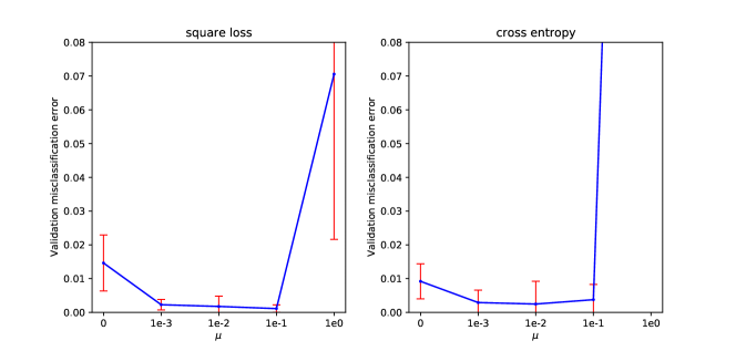
Figure G.3: The errorbar plot of validation misclassification rate with respect to different $\mu$ in the separable case.

Figure G.4: An instance about the training process of SL-ONN + $\ell_{2}$ (Left), CE-ONN + $\ell_{2}$ (Center)  and CE-ONN (Right).

As mentioned in Section 5, we also consider the cross-entropy loss based ONN without $\ell_{2}$ regularization (CE-ONN). All three models are trained for 10000 iterations and achieve 0% training misclassification rate. In Figure G.5, we present five more examples about the decision boundary prediction and test accuracy of SL-ONN + $\ell_{2}$, CE-ONN + $\ell_{2}$ and CE-ONN. We can find that SL-ONN + $\ell_{2}$ still beats CE-ONN + $\ell_{2}$ and CE-ONN in almost all the cases. SL-ONN + $\ell_{2}$ attains the smallest misclassification rate and depicts the largest margin decision boundary which separates the positive and negative samples best. In addition, we can observe that CE-ONN + $\ell_{2}$ outperforms CE-ONN in all cases, although the $\ell_{2}$ regularization term bring some oscillation to the training of CE-ONN + $\ell_{2}$, as shown in Figure G.4.

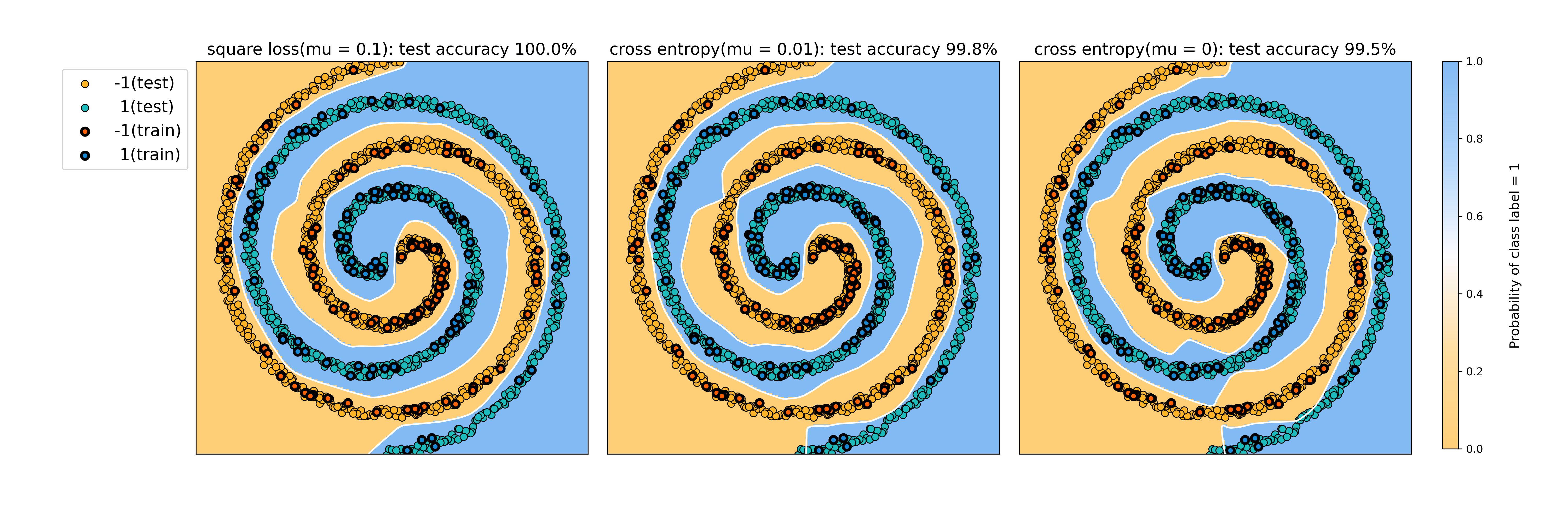
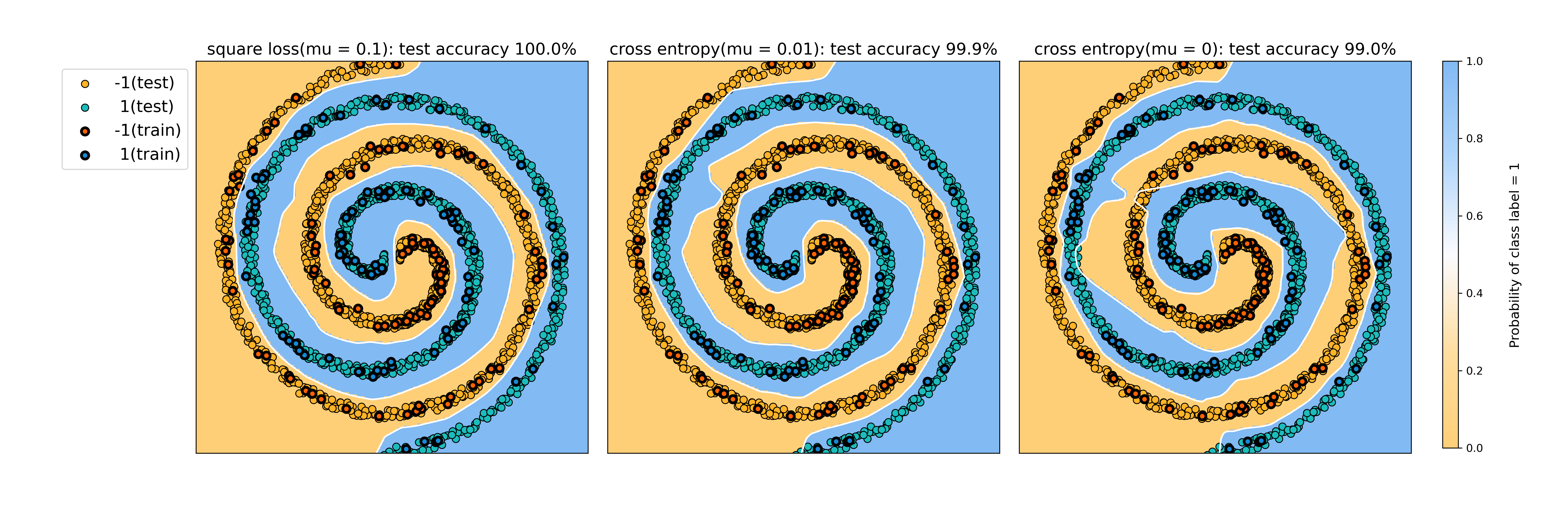
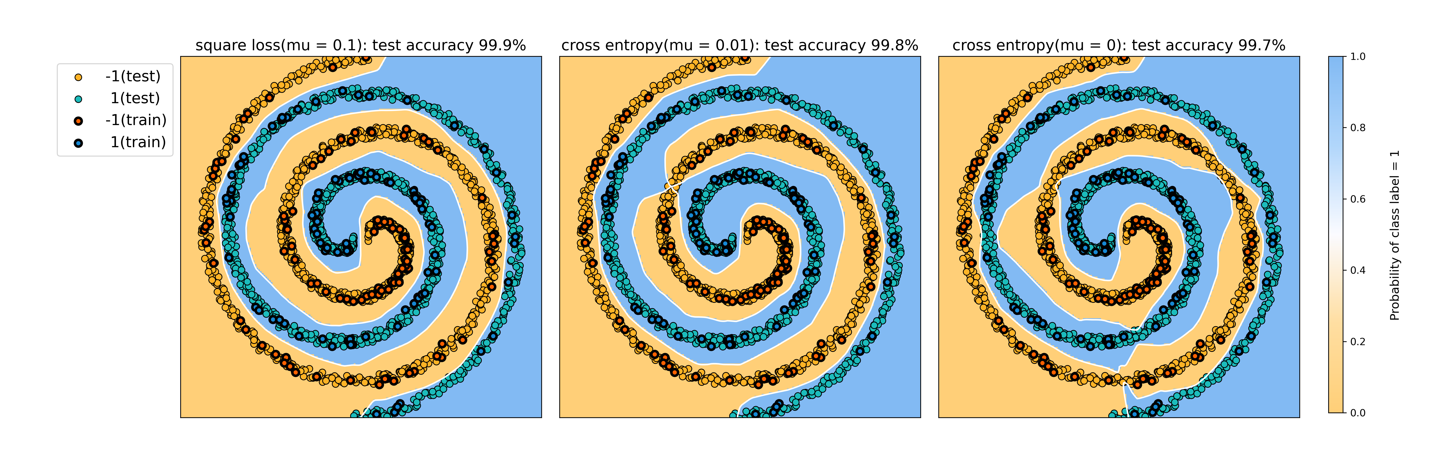
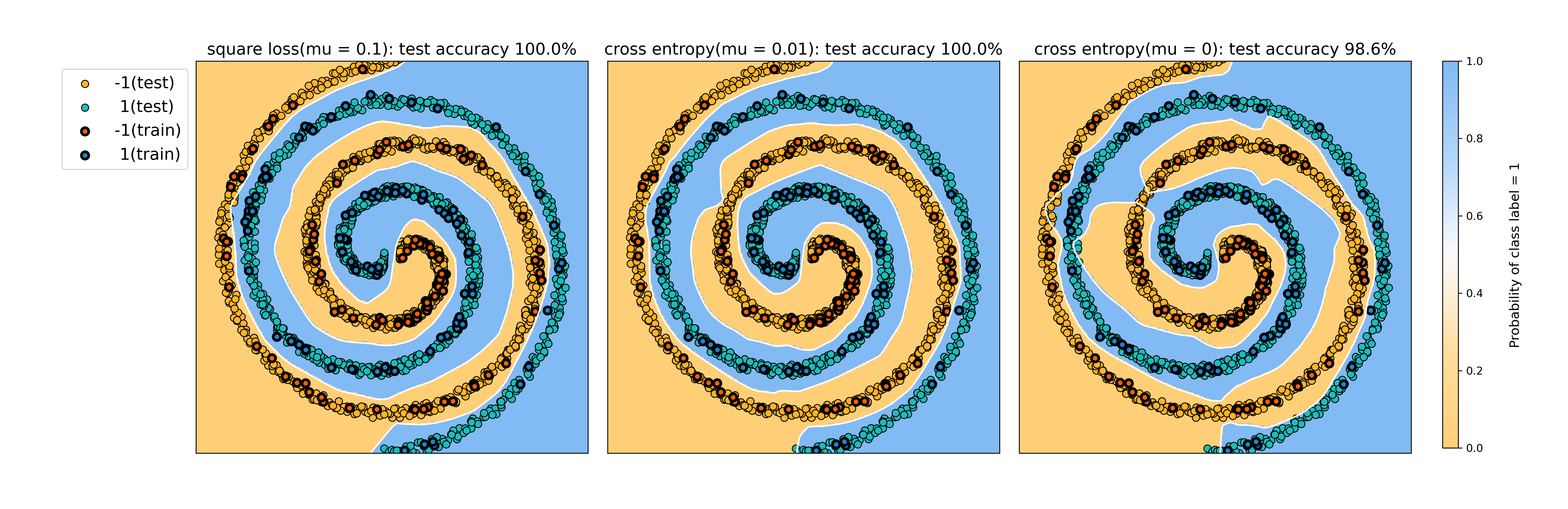
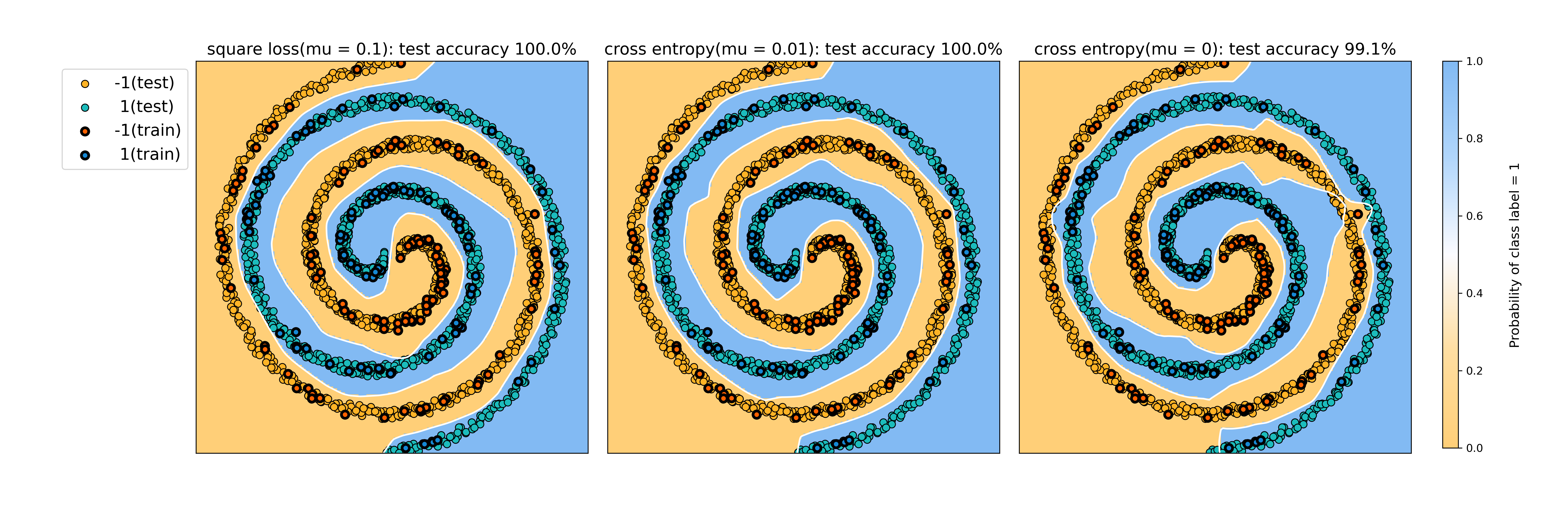
Figure G.5: Five examples of the separable case.

Non-separable case In the non-separable case, the training data points ${\bm{x}}_{1},\cdots,{\bm{x}}_{n}$ are i.i.d. sampled from unif$([-1,1]^{2})$ and the training labels ${y}_{1},\cdots,{y}_{n}$ are sampled according to $Bernoulli(\eta({\bm{x}}_{i}))$, where $\eta(\bm{x})=\sin(\sqrt{2}\pi||\bm{x}||_{2})$, and $n=8000$. The 3-dimensional plot of $\eta({\bm{x}})$ is presented in Figure G.6.

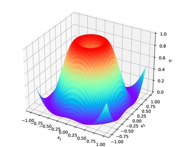
Figure G.6: The 3-dimensional plot of $\eta(\bm{x})$ in the non-separable case.

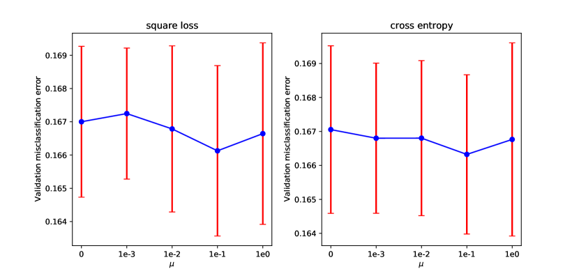
Figure G.7: The errorbar plot of validation misclassification rate with respect to different $\mu$ in the non-separable case.

We select the tuning parameter $\mu$ for SL-ONN + $\ell_{2}$ and CE-ONN + $\ell_{2}$ via a validation set, and the candidate set of $\mu$ is $\{0,0.001,0.01,0.1,1\}$. For each $\mu$, we run 40 replications to estimate the mean and standard deviation of validation misclassification rate. The iteration number of training is 2000. We find SL-ONN + $\ell_{2}$ and CE-ONN + $\ell_{2}$ have the smallest mean and standard deviation for the validation misclassification rate at $\mu=0.1$ and $\mu=0.1$, respectively. The error bar plot for $\mu$ equaling to 0, 0.001, 0.01, 0.1 and 1 is shown in Figure G.7.

The calibration error results are presented in Figure G.8. The error bar plot of the test calibration error shows that $\widehat{f}_{l2}$ has the smaller mean and standard deviation than $\widehat{f}_{ce}$.

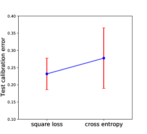
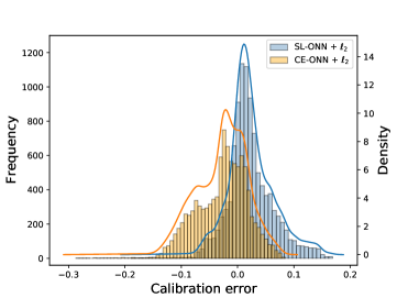
Figure G.8: (Left) The error bar plot of test calibration errors for the 40 replicated runs. (Right) The histogram and kernel density estimation of test calibration errors in one instance from 40 replications. In this instance, $||(\widehat{f}_{l2}+1)/2-\eta||_{L_{\infty}}$ = 0.188, $||(\widehat{f}_{ce}+1)/2-\eta||_{L_{\infty}}$ = 0.287, and the test misclassification rate for $\widehat{f}_{l2}$ and $\widehat{f}_{ce}$ are 0.167 and 0.164, respectively.

G.2 Real Data

Data and network architecture

We use the popular CIFAR-10 and CIFAR-100 datasets, with training and testing split of 50000 and 10000. The data loader is from torch.utils.data. As typically employed in practice, our training includes data augmentations, a composition of random crop and horizontal flip. We trained two types of neural networks, ResNet [39] and Wide ResNet [40]. To be more specific, we used the default ResNet-18 and ResNet-50 for CIFAR-10 and CIFAR-100 respectively, and the default WRN-16-10 for both CIFAR-10 and CIFAR-100. All experiments are run in PyTorch version 1.9.0 and cuda 10.2.

Training details

The training algorithm is the default SGD with momentum ($0.9$) and weight decay ($0.0005$). The learning rate scheduler is the StepLR() from torch.optim.lr_scheduler with step size 50. In our experiment, the only parameters that we tuned are the learning rate (lr) and batch size (bs), with only two options, (lr=0.01, bs=32) and (lr=0.1, bs=128). We find that (lr=0.01, bs=32) performs better for most cases except for square loss trained WRN-16-10 on CIFAR-100, where the average accuracy for (lr=0.01, bs=32) is 77.96%, around 1.5% less than that for (lr=0.1, bs=128). Meanwhile, for cross-entropy trained WRN-16-10, (lr=0.1, bs=128) yields an average accuracy of 76.83%, around 1% less than that for (lr=0.01, bs=32). The two training settings perform quite comparable for WRN-16-10 on CIFAR-10. For consistency, we stick with (lr=0.01, bs=32) in this case.

Adversarial robustness

For square loss, training deep classifiers is the same as regression. When attacking classifiers trained with square loss, the default way of constructing adversarial examples doesn’t work well. To be more specific, for a correctly classified training image $(\bm{x},y)$, the adversarial examples are typically generated by

$$\max_{\left\lVert\bm{\delta}\right\rVert_{\infty}=\alpha}L(f(\bm{x}+\bm{\delta}),y).$$

Such an attacking scheme works fine for cross-entropy, where

$$L(f(\bm{x}),y)=-\log(\mathrm{softmax}(f(\bm{x})))=-\log\left(\frac{\exp(f_{y}(\bm{x}))}{\sum_{k\neq y}\exp(f_{k}(\bm{x}))}\right),$$

but is problematic for regression losses such as square loss. The fundamental reason lies in Proposition 4.1 and its proof. Recall that the conditional probability for square loss consists of projections of the classifier outputs to all the simplex vertices, some of which are sure to be non-positive. The sum of the class probabilities from Equation 4.1 is always 1 but unlike that from softmax function, the summand can be negative. By maximizing the square loss, the resulting “adversarial" image can stay the same class but more confidently. To illustrate, if $f(\bm{x})=\bm{v}_{y}$, the predicted confidence for label $y$ will be 100% and 0 for other classes. The “adversarial" image may be such that $f(\bm{x}+\delta)=2\bm{v}_{y}$, where the predicted label remains unchanged but with an updated confidence of $2-1/K$ for label $y$ and $(1/K-1)/(K-1)<0$ for all other classes. This is obviously not a successful attack.

To this end, we devise a special attacking scheme for classifier trained with square loss and simplex coding. The key idea is to choose attack directions tangent to the sphere inscribed by the simplex. Instead of

$$L(f(\bm{x}),y)=\left\lVert f(\bm{x})-\bm{v}_{y}\right\rVert_{2}^{2},$$

we choose

$$L(f(\bm{x}),y)=\theta(f(\bm{x}),\bm{v}_{y}),$$

where $\theta(\bm{v}_{1},\bm{v}_{2})$ denotes the cosine similarity between $\bm{v}_{1}$ and $\bm{v}_{2}$. We refer to this attack as angle attack.

Empirically, we found our angle attack to significantly outperform the naive attack by maximizing the square loss. For square loss, let the predicted probabilities from Equation 4.1 be $\widehat{\bm{p}}$. Similar to cross entropy, we have also tried two cases of $L(f(\bm{x}),y)$, which corresponds to

$$L_{1}(f(\bm{x}),y)=-\log(\mathrm{softmax}(\widehat{p}_{y}(\bm{x})))\quad\mbox{and}\quad L_{2}(f(\bm{x}),y)=-\log(\widehat{p}_{y}(\bm{x})).$$

Interestingly for PGD-100, $L_{1}$ performs the best, beating angle attack for the majority cases, except for attacking WRN-16-10 on CIFAR-100 with strength 2/255. The reported adversarial accuracy for square loss trained classifiers in Table 1 is by $L_{1}(f(\bm{x}),y)=-\log(\mathrm{softmax}(\widehat{p}_{y}(\bm{x})))$.

The PGD attack results may be further improved for square loss. Nonetheless, the AutoAttack still provides convincing results, as it includes both white-box and black-box attacks. We used the standard version which includes 4 types of attacks, APGD-CE, APGD-DLR, FAB and Square Attack as in [42].

Robustness to Gaussian Noise

To make the robustness evaluation more comprehensive, beyond the adversarial robustness, we also investigate the classifier’s robustness to Gaussian noise injections. With the image pixels’ value normalized to 0 and 1, we consider injecting Gaussian noises to test images and report the test accuracy. The noise standard deviation ranges from 0.1 to 0.4. The test accuracy results for both CIFAR-10 and CIFAR-100 are listed in Table G.3.

Table G.3: Black-box Gaussian noise robustness results. The reported accuracy is the average of 5 replications.

Dataset	Network	Loss	Gaussian noise standard deviation
			0.00	0.10	0.20	0.30	0.40
CIFAR-10	ResNet-18	SL	95.04	90.07	70.16	42.13	25.38
		CE	95.15	90.03	69.71	41.08	24.66
	WRN-16-10	SL	95.02	88.49	60.91	35.78	24.04
		CE	93.94	84.78	56.63	33.70	22.41
CIFAR-100	ResNet-50	SL	78.91	63.06	36.64	17.78	9.47
		CE	79.82	62.72	34.42	16.69	9.11
	WRN-16-10	SL	79.65	62.01	30.69	15.11	8.88
		CE	77.89	60.14	26.47	10.26	5.57

Simplex coding vs. one-hot coding

The one-hot coding is the usual choice for applying square loss to classification. However, it is empirically observed to struggle when the number of classes are large. For a single training data point $\bm{x}$ and label $k$, Hui and Belkin [4] proposed to modify the training objective from the typical $(f_{k}({\bm{x}})-1)^{2}+\sum_{i\neq k}f_{i}({\bm{x}})^{2}$ to $J\cdot(f_{k}({\bm{x}})-M)^{2}+\sum_{i\neq k}f_{i}({\bm{x}})^{2}$, where $J,M$ are hyperparameters to make $f_{k}$ more prominent in the loss. Similar modification is also proposed in [5]. The scaling trick involves two hyperparameters, which can be hard to tune. We evaluate the two coding schemes in our experiment setting and the results are summarized in Table G.4. The test accuracy for scaled one-hot coding scheme performs comparably for ResNet-18 on CIFAR-10 and ResNet-50 on CIFAR-100. For WRN-16-10, the simplex coding performs better.

Table G.4: Test accuracy for square loss with one-hot coding (scaled) (OC) vs. simplex coding (SC). Accuracy with an asteroid sign (^∗) denotes cases where the training accuracy doesn’t overfit after 200 training epochs.

Dataset	Network	One-hot scaling	SGD parameters	OC clean acc(%)	SC clean acc(%)
CIFAR-10	ResNet-18	k=1, M=1	lr=0.01, bs=32	94.95	95.04
			lr=0.1, bs=128	10${}^{*}~{}~{}~{}$	10${}^{*}~{}~{}~{}$
	WRN-16-10	k=1,M =1	lr=0.01, bs=32	89.75∗	95.02
			lr=0.1, bs=128	88.43∗	95.03
CIFAR-100	ResNet-50	k=5, M=15	lr=0.01, bs=32	79.06	78.91
			lr=0.1, bs=128	$1^{*}~{}$	1${}^{*}~{}$
	WRN-16-10	k=5, M=15	lr=0.01, bs=32	78.42	78.06
			lr=0.1, bs=128	78.39	79.65

References

- Yu et al. [2020] Yaodong Yu, Kwan Ho Ryan Chan, Chong You, Chaobing Song, and Yi Ma. Learning diverse and discriminative representations via the principle of maximal coding rate reduction. Advances in Neural Information Processing Systems, 33, 2020.
- Pang et al. [2019] Tianyu Pang, Kun Xu, Yinpeng Dong, Chao Du, Ning Chen, and Jun Zhu. Rethinking softmax cross-entropy loss for adversarial robustness. arXiv preprint arXiv:1905.10626, 2019.
- Guo et al. [2017] Chuan Guo, Geoff Pleiss, Yu Sun, and Kilian Q Weinberger. On calibration of modern neural networks. In International Conference on Machine Learning, pages 1321–1330. PMLR, 2017.
- Hui and Belkin [2020] Like Hui and Mikhail Belkin. Evaluation of neural architectures trained with square loss vs cross-entropy in classification tasks. arXiv preprint arXiv:2006.07322, 2020.
- Demirkaya et al. [2020] Ahmet Demirkaya, Jiasi Chen, and Samet Oymak. Exploring the role of loss functions in multiclass classification. In 2020 54th Annual Conference on Information Sciences and Systems (CISS), pages 1–5. IEEE, 2020.
- Kornblith et al. [2020] Simon Kornblith, Honglak Lee, Ting Chen, and Mohammad Norouzi. Demystifying loss functions for classification. 2020.
- Papyan et al. [2020] Vardan Papyan, XY Han, and David L Donoho. Prevalence of neural collapse during the terminal phase of deep learning training. Proceedings of the National Academy of Sciences, 117(40):24652–24663, 2020.
- Mroueh et al. [2012] Youssef Mroueh, Tomaso Poggio, Lorenzo Rosasco, and Jean-Jacques Slotine. Multiclass learning with simplex coding. arXiv preprint arXiv:1209.1360, 2012.
- Zhang [2004] Tong Zhang. Statistical behavior and consistency of classification methods based on convex risk minimization. The Annals of Statistics, pages 56–85, 2004.
- Zhang et al. [2017] Hongyi Zhang, Moustapha Cisse, Yann N Dauphin, and David Lopez-Paz. mixup: Beyond empirical risk minimization. arXiv preprint arXiv:1710.09412, 2017.
- Hinton et al. [2015] Geoffrey Hinton, Oriol Vinyals, and Jeff Dean. Distilling the knowledge in a neural network. arXiv preprint arXiv:1503.02531, 2015.
- Menon et al. [2021] Aditya K Menon, Ankit Singh Rawat, Sashank Reddi, Seungyeon Kim, and Sanjiv Kumar. A statistical perspective on distillation. In International Conference on Machine Learning, pages 7632–7642. PMLR, 2021.
- Khosla et al. [2020] Prannay Khosla, Piotr Teterwak, Chen Wang, Aaron Sarna, Yonglong Tian, Phillip Isola, Aaron Maschinot, Ce Liu, and Dilip Krishnan. Supervised contrastive learning. arXiv preprint arXiv:2004.11362, 2020.
- Graf et al. [2021] Florian Graf, Christoph Hofer, Marc Niethammer, and Roland Kwitt. Dissecting supervised constrastive learning. In International Conference on Machine Learning, pages 3821–3830. PMLR, 2021.
- Mammen and Tsybakov [1999] Enno Mammen and Alexandre B Tsybakov. Smooth discrimination analysis. The Annals of Statistics, 27(6):1808–1829, 1999.
- Bartlett et al. [2006] Peter L Bartlett, Michael I Jordan, and Jon D McAuliffe. Convexity, classification, and risk bounds. Journal of the American Statistical Association, 101(473):138–156, 2006.
- Audibert and Tsybakov [2007] Jean-Yves Audibert and Alexandre B Tsybakov. Fast learning rates for plug-in classifiers. The Annals of statistics, 35(2):608–633, 2007.
- Kohler and Krzyzak [2007] Michael Kohler and Adam Krzyzak. On the rate of convergence of local averaging plug-in classification rules under a margin condition. IEEE Transactions on Information Theory, 53(5):1735–1742, 2007.
- Steinwart et al. [2007] Ingo Steinwart, Clint Scovel, et al. Fast rates for support vector machines using Gaussian kernels. The Annals of Statistics, 35(2):575–607, 2007.
- Kim et al. [2018] Yongdai Kim, Ilsang Ohn, and Dongha Kim. Fast convergence rates of deep neural networks for classification. arXiv preprint arXiv:1812.03599, 2018.
- Kohler and Langer [2020] Michael Kohler and Sophie Langer. Statistical theory for image classification using deep convolutional neural networks with cross-entropy loss. arXiv preprint arXiv:2011.13602, 2020.
- Ji and Telgarsky [2019] Ziwei Ji and Matus Telgarsky. Polylogarithmic width suffices for gradient descent to achieve arbitrarily small test error with shallow ReLU networks. arXiv preprint arXiv:1909.12292, 2019.
- Hu et al. [2020] Wei Hu, Zhiyuan Li, and Dingli Yu. Simple and effective regularization methods for training on noisily labeled data with generalization guarantee. In International Conference on Learning Representations, 2020.
- Cao and Gu [2019] Yuan Cao and Quanquan Gu. Generalization bounds of stochastic gradient descent for wide and deep neural networks. Advances in Neural Information Processing Systems, 32:10836–10846, 2019.
- Cao and Gu [2020] Yuan Cao and Quanquan Gu. Generalization error bounds of gradient descent for learning over-parameterized deep relu networks. In Proceedings of the AAAI Conference on Artificial Intelligence, volume 34, pages 3349–3356, 2020.
- Han et al. [2021] XY Han, Vardan Papyan, and David L Donoho. Neural collapse under mse loss: Proximity to and dynamics on the central path. arXiv preprint arXiv:2106.02073, 2021.
- Muthukumar et al. [2020] Vidya Muthukumar, Adhyyan Narang, Vignesh Subramanian, Mikhail Belkin, Daniel Hsu, and Anant Sahai. Classification vs regression in overparameterized regimes: Does the loss function matter? arXiv preprint arXiv:2005.08054, 2020.
- Poggio and Liao [2019] Tomaso Poggio and Qianli Liao. Generalization in deep network classifiers trained with the square loss. Technical report, CBMM Memo No, 2019.
- Jacot et al. [2018] Arthur Jacot, Franck Gabriel, and Clément Hongler. Neural tangent kernel: Convergence and generalization in neural networks. In Advances in Neural Information Processing Systems, pages 8571–8580, 2018.
- Arora et al. [2019] Sanjeev Arora, Simon S Du, Wei Hu, Zhiyuan Li, and Ruosong Wang. Fine-grained analysis of optimization and generalization for overparameterized two-layer neural networks. arXiv preprint arXiv:1901.08584, 2019.
- Bietti and Mairal [2019] Alberto Bietti and Julien Mairal. On the inductive bias of neural tangent kernels. arXiv preprint arXiv:1905.12173, 2019.
- Hu et al. [2021] Tianyang Hu, Wenjia Wang, Cong Lin, and Guang Cheng. Regularization matters: A nonparametric perspective on overparametrized neural network. In International Conference on Artificial Intelligence and Statistics, pages 829–837. PMLR, 2021.
- Elsayed et al. [2018] Gamaleldin F Elsayed, Dilip Krishnan, Hossein Mobahi, Kevin Regan, and Samy Bengio. Large margin deep networks for classification. arXiv preprint arXiv:1803.05598, 2018.
- Ding et al. [2018] Gavin Weiguang Ding, Yash Sharma, Kry Yik Chau Lui, and Ruitong Huang. Mma training: Direct input space margin maximization through adversarial training. arXiv preprint arXiv:1812.02637, 2018.
- Geifman et al. [2020] Amnon Geifman, Abhay Yadav, Yoni Kasten, Meirav Galun, David Jacobs, and Ronen Basri. On the similarity between the Laplace and neural tangent kernels. arXiv preprint arXiv:2007.01580, 2020.
- Chen and Xu [2020] Lin Chen and Sheng Xu. Deep neural tangent kernel and Laplace kernel have the same RKHS. arXiv preprint arXiv:2009.10683, 2020.
- He et al. [2019] Zhezhi He, Adnan Siraj Rakin, and Deliang Fan. Parametric noise injection: Trainable randomness to improve deep neural network robustness against adversarial attack. In Proceedings of the IEEE/CVF Conference on Computer Vision and Pattern Recognition, pages 588–597, 2019.
- Fang et al. [2021] Cong Fang, Hangfeng He, Qi Long, and Weijie J Su. Exploring deep neural networks via layer-peeled model: Minority collapse in imbalanced training. Proceedings of the National Academy of Sciences, 118(43), 2021.
- He et al. [2016] Kaiming He, Xiangyu Zhang, Shaoqing Ren, and Jian Sun. Deep residual learning for image recognition. In Proceedings of the IEEE Conference on Computer Vision and Pattern Recognition, pages 770–778, 2016.
- Zagoruyko and Komodakis [2016] Sergey Zagoruyko and Nikos Komodakis. Wide residual networks. arXiv preprint arXiv:1605.07146, 2016.
- Madry et al. [2017] Aleksander Madry, Aleksandar Makelov, Ludwig Schmidt, Dimitris Tsipras, and Adrian Vladu. Towards deep learning models resistant to adversarial attacks. arXiv preprint arXiv:1706.06083, 2017.
- Croce and Hein [2020] Francesco Croce and Matthias Hein. Reliable evaluation of adversarial robustness with an ensemble of diverse parameter-free attacks. In International Conference on Machine Learning, pages 2206–2216. PMLR, 2020.
- Vaicenavicius et al. [2019] Juozas Vaicenavicius, David Widmann, Carl Andersson, Fredrik Lindsten, Jacob Roll, and Thomas Schön. Evaluating model calibration in classification. In The 22nd International Conference on Artificial Intelligence and Statistics, pages 3459–3467. PMLR, 2019.
- Du et al. [2018] Simon S Du, Xiyu Zhai, Barnabas Poczos, and Aarti Singh. Gradient descent provably optimizes over-parameterized neural networks. arXiv preprint arXiv:1810.02054, 2018.
- Edmunds and Triebel [2008] David Eric Edmunds and Hans Triebel. Function Spaces, Entropy Numbers, Differential Operators, volume 120. Cambridge University Press, 2008.
- Nitanda and Suzuki [2020] Atsushi Nitanda and Taiji Suzuki. Optimal rates for averaged stochastic gradient descent under neural tangent kernel regime. arXiv preprint arXiv:2006.12297, 2020.
- Schmidt-Hieber [2020] Johannes Schmidt-Hieber. Nonparametric regression using deep neural networks with relu activation function. The Annals of Statistics, 48(4):1875–1897, 2020.
- Farrell et al. [2021] Max H Farrell, Tengyuan Liang, and Sanjog Misra. Deep neural networks for estimation and inference. Econometrica, 89(1):181–213, 2021.
- Nitanda et al. [2019] Atsushi Nitanda, Geoffrey Chinot, and Taiji Suzuki. Gradient descent can learn less over-parameterized two-layer neural networks on classification problems. arXiv preprint arXiv:1905.09870, 2019.
- Li and Liang [2018] Yuanzhi Li and Yingyu Liang. Learning overparameterized neural networks via stochastic gradient descent on structured data. In Advances in Neural Information Processing Systems, pages 8157–8166, 2018.
- Aronszajn [1950] N. Aronszajn. Theory of reproducing kernels. Trans. Amer. Math. Soc., 68(3):337–404, 1950.
- Bennett and Sharpley [1988] Colin Bennett and Robert C Sharpley. Interpolation of Operators. Academic press, 1988.
- Wendland [2004] Holger Wendland. Scattered Data Approximation. Cambridge University Press, 2004.