Scaling Structured Inference with Randomization

Abstract

Deep discrete structured models have seen considerable progress recently, but traditional inference using dynamic programming (DP) typically works with a small number of states (less than hundreds), which severely limits model capacity. At the same time, across machine learning, there is a recent trend of using randomized truncation techniques to accelerate computations involving large sums. Here, we propose a family of randomized dynamic programming (RDP) algorithms for scaling structured models to tens of thousands of latent states. Our method is widely applicable to classical DP-based inference (partition function, marginal, reparameterization, entropy) and different graph structures (chains, trees, and more general hypergraphs). It is also compatible with automatic differentiation: it can be integrated with neural networks seamlessly and learned with gradient-based optimizers. Our core technique approximates the sum-product by restricting and reweighting DP on a small subset of nodes, which reduces computation by orders of magnitude. We further achieve low bias and variance via Rao-Blackwellization and importance sampling. Experiments over different graphs demonstrate the accuracy and efficiency of our approach. RDP can also be used to learn a structured variational autoencoder with a scaled inference network which outperforms baselines in terms of test likelihood and successfully prevents collapse.

1 Introduction

Table 1: Dynamic programming algorithms for different inference over different graphs. Our randomization technique covers a spectrum of classical DP algorithms on different graphs. Scaled algorithms shown in red are randomized in this work.

Graph	Model	Partition & Marginal	Entropy	Sampling & Reparameterization
Chains	HMM, CRF, Semi-Markov	Forward-Backward	Backward Entropy	Gumbel Sampling (Fu et al., 2020)
Hypertrees	PCFG, Dependency CRF	Inside-Outside	Outside Entropy	Stochastic Softmax (Paulus et al., 2020)
General graph	General Exponential Family	Sum-Product	Bethe Entropy	Stochastic Softmax (Paulus et al., 2020)

Deep discrete structured models (Martins et al., 2019; Rush, 2020) have enjoyed great progress recently, improving performance and interpretability in a range of tasks including sequence tagging (Ma & Hovy, 2016), parsing (Zhang et al., 2020; Yang et al., 2021), and text generation (Wiseman et al., 2018). However, their capacity is limited by issues of scaling (Sun et al., 2019; Chiu & Rush, 2020; Yang et al., 2021; Chiu et al., 2021). Traditional dynamic programming based inference for exponential families has limited scalability with large combinatorial spaces. When integrating exponential families with neural networks (e.g., a VAE with a CRF inference network, detailed later), the small latent combinatorial space severely restricts model capacity. Existing work has already observed improved performance by scaling certain types of structures (Yang et al., 2021; Li et al., 2020; Chiu & Rush, 2020), and researchers are eager to know if there are general techniques for scaling classical structured models.

Challenges in scaling structured models primarily come from memory complexity. For example, consider linear-chain CRFs (Sutton & McCallum, 2006), the classical sequence model that uses the Forward algorithm, a dynamic programming algorithm, for computing the partition function exactly. This algorithm requires $O(TN^{2})$ computation where $N$ is the number of latent states and $T$ is the length of the sequence. It is precisely the $N^{2}$ term that is problematic in terms of memory and computation. This limitation is more severe under automatic differentiation (AD) frameworks as all intermediate DP computations are stored for gradient construction. Generally, DP-based inference algorithms are not optimized for modern computational hardware like GPUs and typically work under small-data regimes, with $N$ in the range [10, 100] (Ma & Hovy, 2016; Wiseman et al., 2018). With larger $N$, inference becomes intractable since the computation graph does not easily fit into GPU memory (Sun et al., 2019).

Aligning with a recent trend of exploiting randomization techniques for machine learning problems (Oktay et al., 2020; Potapczynski et al., 2021; Beatson & Adams, 2019), this work proposes a randomization framework for scaling structured models, which encompasses a family of randomized dynamic programming algorithms with a wide coverage of different structures and inference (Table 1). Within our randomization framework, instead of summing over all possible combinations of latent states, we only sum over paths with the most probable states and sample a subset of less likely paths to correct the bias according to a reasonable proposal. Since we only calculate the chosen paths, memory consumption can be reduced to a reasonably small budget. We thus recast the computation challenge into a tradeoff between memory budget, proposal accuracy, and estimation error. In practice, we show RDP scales existing models by two orders of magnitude with memory complexity as small as one percent.

In addition to the significantly increased scale, we highlight the following advantages of RDP: (1) applicability to different structures (chains, trees, and hypergraphs) and inference operations (partition function, marginal, reparameterization, and entropy); (2) compatibility with automatic differentiation and existing efficient libraries (like Torch-Struct in Rush, 2020); and (3) statistically principled controllability of bias and variance. As a concrete application, we show that RDP can be used for learning a structured VAE with a scaled inference network. In experiments, we first demonstrate that RDP algorithms estimate partition function and entropy for chains and hypertrees with lower mean square errors than baselines. Then, we show their joint effectiveness for learning the scaled VAE. RDP outperforms baselines in terms of test likelihood and successfully prevents posterior collapse. Our implementation is at https://github.com/FranxYao/RDP.

2 Background and Preliminaries

Problem Statement We start with a widely-used structured VAE framework. Let ${\bm{y}}$ be an observed variable. Let ${\bm{X}}$ be any latent structure (sequences of latent tags, parse trees, or general latent graphs, see Table 1) that generates ${\bm{y}}$. Let $p_{\psi}$ denote the generative model, and $q_{\theta}$ the inference model. We optimize:

$$\mathcal{L}=\mathbb{E}_{q_{\theta}({\bm{X}}|{\bm{y}})}[\log p_{\psi}({\bm{X}},{\bm{y}})-\log q_{\theta}({\bm{X}}|{\bm{y}})]$$ (1)

where the inference model $q_{\theta}$ takes the form of a discrete undirected exponential family (e.g., linear-chain CRFs in Fu et al., 2020). Successful applications of this framework include sequence tagging (Mensch & Blondel, 2018), text generation (Li & Rush, 2020), constituency parsing (Kim et al., 2019), dependency parsing (Corro & Titov, 2018), latent tree induction (Paulus et al., 2020), and so on. Our goal is to learn this model with a scaled latent space (e.g., a CRF encoder with tens of thousands of latent states).

Sum-Product Recap Learning models in Eq. 1 usually requires classical sum-product inference (and its variants) of $q_{\theta}$, which we now review. Suppose $q_{\theta}$ is in standard overparameterization of a discrete exponential family (Wainwright & Jordan, 2008):

$$q_{\theta}({\bm{X}})\propto\exp\left\{\sum_{s\in V}\phi_{s}(x_{s})+\sum_{(s,t)\in E}\phi_{st}(x_{s},x_{t})\right\}$$ (2)

where ${\bm{X}}=[X_{1},...,X_{M}]$ is a random vector of nodes in a graphical model with each node taking discrete values $X_{i}\in\{1,2,...,N\}$, $N$ is the number of states, $\phi_{st}$ is the edge potential, and $\phi_{s}$ is the node potential. Here, we use a general notation of nodes $V$ and edges $E$. We discuss specific structures later. Suppose we want to compute its marginals and log partition function. The solution is the sum-product algorithm that recursively updates the message at each edge:

$$\mu_{ts}(x_{s})\propto\sum_{x_{t}^{\prime}=1}^{N}\Big{\{}\phi_{st}(x_{s},x_{t}^{\prime})\phi_{t}(x_{t}^{\prime})\prod_{u\in V_{t}^{s}}\mu_{ut}(x_{t}^{\prime})\Big{\}}$$ (3)

where $\mu_{ts}(x_{s})$ denotes the message from node $t$ to node $s$ evaluated at $X_{s}=x_{s}$, $V_{t}^{s}$ denotes the set of neighbor nodes of $t$ except $s$. Upon convergence, it gives us the Bethe approximation (if the graph is loopy) of the marginal, partition function, and entropy (as functions of the edge marginals $\mu_{ts}$). These quantities are then used in gradient based updates of the potentials $\phi$ (detailed in Sec. 4). When the underlying graph is a tree, this approach becomes exact and convergence is linear in the number of edges.

Challenges in Scaling The challenge is how to scale the sum-product computation for $q_{\theta}$. Specifically, gradient-based learning requires three types of inference: (a) partition estimation (for maximizing likelihood); (b) re-parameterized sampling (for gradient estimation); and (c) entropy estimation (for regularization). Existing sum-product variants (Table 1) provide exact solutions, but only for a small latent space (e.g., a linear-chain CRF with state number smaller than 100). Since the complexity of DP-based inference is usually at least quadratic to the size of the latent states, it would induce memory overflow if we wanted to scale it to tens of thousands.

Restrictions from Automatic Differentiation At first sight, one may think the memory requirement for some algorithms is not so large. For example, the memory complexity of a batched forward sum-product (on chains) is $O(BTN^{2})$. Consider batch size $B=10$, sequence length $T=100$, number of states $N=1000$, then the complexity is $O(10^{9})$, which seems acceptable, especially given multiple implementation tricks (e.g., dropping the intermediate variables). However, this is not the case under automatic differentiation, primarily because AD requires storing all intermediate computations for building the adjacent gradient graph. This not only invalidates tricks like dropping intermediate variables (because they should be stored) but also multiplies memory complexity when building the adjacent gradient graph (Eisner, 2016). This problem is more severe if we want to compute higher-order gradients, or if the underlying DP has higher-order complexity (e.g., the Inside algorithm of cubic complexity $O(T^{2}N^{3})$). Since gradient-based optimization requires AD-compatibility, scaling techniques are under similar restrictions, namely storing all computations to construct the adjacent gradient graph.

Previous Efforts Certainly there exist several excellent scaling techniques for structured models, though most come with some intrinsic limitations that we hope to alleviate. In addition to AD-compatibility restrictions, many existing techniques either require additional assumptions (e.g., sparsity in Lavergne et al., 2010; Sokolovska et al., 2010; Correia et al., 2020, pre-clustering in Chiu & Rush, 2020, or low-rank in Chiu et al., 2021), rely on handcrafted heuristics for bias correction (Jeong et al., 2009), or cannot be easily adapted to modern GPUs with tensorization and parallelization (Klein & Manning, 2003). As a result, existing methods apply to a limited range of models: Chiu & Rush (2020) only consider chains and Yang et al. (2021) only consider probabilistic context-free grammars (PCFGs).

One notably promising direction comes from Sun et al. (2019), where they consider topK computation and drop all low probability states. NEURIPS2018_6211080f also considered topK inference in a smoothed setting (where they have more theoretical analytics but are less about memory efficiency) and their topK inference also points to efficiency improvements. While intuitively sensible (indeed we build on this idea here), their deterministic truncation induces severe bias (later shown in our experiments). As we will discuss, this bias can be effectively mitigated by randomization.

Randomization of Sums in Machine Learning Randomization is a long-standing technique in machine learning (Mahoney, 2011; Halko et al., 2011) and has been applied to dynamic programs before the advent of deep learning (Bouchard-côté et al., 2009; Blunsom & Cohn, 2010). Notably, works like koller1999general; pmlr-v5-ihler09a also consider sampling techniques for sum-product inference. However, since these methods are proposed before deep learning, their differentiability remain untested. More recently, randomization has been used in the context of deep learning, including density estimation (Rhodes et al., 2020), Gaussian processes (Potapczynski et al., 2021), automatic differentiation (Oktay et al., 2020), gradient estimation (Correia et al., 2020), and optimization (Beatson & Adams, 2019). The foundation of our randomized DP also lies in speeding up summation by randomization. To see the simplest case, consider the sum of a sorted list ${\bm{a}}$ of positive numbers: $S=\sum_{i=1}^{N}a_{i}$. This requires $N-1$ additions, which could be expensive when $N$ is large. Suppose one would like to reduce the number of summands to $K$, Liu et al. (2019) discusses the following sum-and-sample estimator for gradient estimation:

$$\hat{S} =\sum_{i=1}^{K_{1}}a_{i}+\frac{1}{K_{2}}\sum_{j=1}^{K_{2}}\frac{a_{\delta_{j}}}{q_{\delta_{j}}}$$ (4)

where $K_{1}+K_{2}=K$ and $\delta_{j}\sim{\bm{q}}=[q_{K_{1}+1},...,q_{N}]$, ${\bm{q}}$ is a proposal distribution upon the tail summands $[a_{K_{1}+1},...,a_{N}]$. This estimator is visualized in Fig. 1A. One can show that it is unbiased: $\mathbb{E}_{\bm{q}}[\hat{S}]=S$, irrespective of how we choose the proposal ${\bm{q}}$. The oracle proposal ${\bm{q}}^{\star}$is the normalized tail summands: $q_{i}^{\star}=a_{i}/\sum_{j=K_{1}+1}^{N}a_{j}$, under which the estimate becomes exact: $\hat{S}\equiv S$. Note that the bias is corrected by dividing the proposal probability.

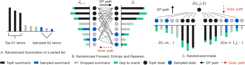
Figure 1: Scaling inference by randomization. (A): randomized summation (Eq.4). (B): Randomized Forward (Alg. 1) recursively applies randomized summation at each DP step. Memory reduction is achieved by restricting computation on edges linking the sampled nodes. Second-order randomized DPs (Entropy and Reparameterization, Alg. 3 and 4) reuse this graph and share the same path as the gradients. (C): Randomized Inside (Alg. 2) applies randomized summation twice at each DP step. All algorithms in our randomized DP family are compatible to automatic differentiation, the direction of the gradient is shown by red dashed arrows.

3 Scaling Inference with Randomization

In this section, we introduce our randomized dynamic programming algorithms. We first introduce a generic randomized sum-product framework for approximating the partition function of any graph structure. Then we instantiate this framework on two classical structures, chains and hypertrees, respectively. When running the randomized sum-product in a left-to-right (or bottom-up) order, we get a randomized version of the classicial Forward (or Inside) algorithm for estimating the partition function for chains like HMMs and Linear-chain CRFs (or hypertrees like PCFGs and Dependency CRFs in Kim et al., 2019). We call these two algorithms first-order RDPs because they run the computation graph in one pass. Next, we generalize RDP to two more inference operations (beyond partition estimation): entropy estimation (for the purposes of regularized training) and reparameterization (for gradient-based optimization). We collectively use the term second-order RDPs to refer to entropy and reparameterization algorithms because they call first-order RDPs as a subroutine and run a second pass of computation upon the first-order graphs. We will compose these algorithms into a structured VAE in Sec. 4.

3.1 Framework: Randomized Sum-Product

Our key technique for scaling the sum-product is a randomized message estimator. Specifically, for each node $X_{t}$, given a pre-constructed proposal ${\bm{q}}_{t}=[q_{t}(1),...,q_{t}(N)]$ (we discuss how to construct a correlated proposal later because it depends on the specific neural parameterization), we retrieve the top $K_{1}$ index $\{\sigma_{t,i}\}_{i=1}^{K_{1}}$ from ${\bm{q}}_{t}$, and get a $K_{2}$-sized sample $\{\delta_{t,i}\}_{i=1}^{K_{2}}$ from the rest of ${\bm{q}}_{t}$:

$$[\sigma_{t,1},...,\sigma_{t,K_{1}},...,\sigma_{t,N}]=\arg\text{sort}\{q_{t}(i)\}_{i=1}^{N}$$ (5)

$$\delta_{t,j}\overset{\text{i.i.d.}}{\sim}\text{Categorical}\{q_{t}(\sigma_{t,K_{1}+1}),...,q_{t}(\sigma_{t,N})\}$$ (6)

$$\Omega_{t}^{K_{1}}=\{\sigma_{t,i}\}_{i=1}^{K_{1}}\quad\quad\Omega_{t}^{K_{2}}=\{\delta_{t,j}\}_{j=1}^{K_{2}}$$ (7)

Then, we substitute the full index $\{1,...,N\}$ with the the top $\Omega_{t}^{K_{1}}$ and the sampled index $\Omega_{t}^{K_{2}}$:

$$\hat{\mu}_{ts}(x_{s})\propto\sum_{\sigma_{t}\in\Omega_{t}^{K_{1}}}\Big{\{}\phi_{st}(x_{s},\sigma_{t})\phi_{t}(\sigma_{t})\prod_{u\in V_{t}^{s}}\hat{\mu}_{ut}(\sigma_{t})\Big{\}}+$$

$$\sum_{\delta_{t}\in\Omega_{t}^{K_{2}}}\Big{\{}\frac{1}{K_{2}q_{t}(\delta_{t})}\phi_{st}(x_{s},\delta_{t})\phi_{t}(\delta_{t})\prod_{u\in V_{t}^{s}}\hat{\mu}_{ut}(\delta_{t})\Big{\}}$$ (8)

where the oracle proposal is proportional to the actual summands (Eq. 3). Here indices are pre-computed outside DP. This means the computation of Eq. 5–7 can be moved outside the AD engine (e.g., in Pytorch, under the no_grad statement) to further save GPU memory usage.

We now show that estimator Eq. 8 can be interpreted as a combination of Rao-Blackwellization (RB) and importance sampling (IS). Firstly, RB says that a function $J(X,Y)$ depending on two random variables $X,Y$ has larger variance than its conditional expectation $\hat{J}(X)=\mathbb{E}[J(X,Y)|X]$ (Ranganath et al., 2014):

$$\mathbb{V}[\hat{J}(X)] =\mathbb{V}[J(X,Y)]-\mathbb{E}[(J(X,Y)-\hat{J}(X))^{2}]$$ (9)

$$\leq\mathbb{V}[J(X,Y)]$$ (10)

This is because $Y$ has been integrated out and the source of randomness is reduced to $X$. Now let $\delta_{1},\delta_{2}$ be uniform random indices taking values from $\Omega_{t}^{K_{1}}$ and $\Omega_{t}^{K_{2}}$, respectively. Consider a simple unbiased estimate $S$ for the message $\mu_{st}$:

$$m_{st}(i) =\phi_{st}(x_{s},i)\phi_{t}(i)\prod_{u\in V_{t}^{s}}\mu_{ut}(i)$$ (11)

$$S(\delta_{1},\delta_{2}) =K_{1}m_{st}(\delta_{1})+(N-K_{1})m_{st}(\delta_{2})$$ (12)

The conditional expectation $\hat{S}(\delta_{2})=\mathbb{E}[S(\delta_{1},\delta_{2})|\delta_{2}]$ is:

$$\hat{S}(\delta_{2})=\sum_{\sigma_{t}\in\Omega_{t}^{K_{1}}}m_{st}(\sigma_{t})+(N-K_{1})m_{st}(\delta_{2})$$ (13)

Plugging $S(\delta_{1},\delta_{2}),\hat{S}(\delta_{2})$ in Eq. 10, we get variance reduction: $\mathbb{V}[\hat{S}(\delta_{2})]\leq\mathbb{V}[S(\delta_{1},\delta_{2})]$. Note that the variance will becomes smaller as $K_{1}$ becomes larger. Now change $\delta_{2}$ in Eq. 13 to from the proposal in Eq. 6 then take expectation:

$$\mathbb{E}_{\delta_{2}\sim\text{Uniform}(\Omega_{t}^{K_{2}})}[(N-K_{1})m_{st}(\delta_{2})]$$ (14)

$$=\mathbb{E}_{\delta_{2}\sim{\bm{q}}_{t}}[\frac{1}{q_{t}(\delta_{2})(N-K_{1})}(N-K_{1})m_{st}(\delta_{2})]$$ (15)

$$=\mathbb{E}_{\delta_{2}\sim{\bm{q}}_{t}}[\frac{1}{q_{t}(\delta_{2})}m_{st}(\delta_{2})]$$ (16)

This is an instance of importance sampling where the importance weight is $\frac{1}{q_{t}(\delta_{2})(N-K_{1})}$. Variance can be reduced if ${\bm{q}}_{t}$ is correlated with the summands (Eq. 11). Finally, combining Eq. 16 and 13 and increasing the number of sampled index $\delta_{2}$ to $K_{2}$ will recover our full message estimator in Eq. 8.

Algorithm 1 Randomized Forward

  Input: potentials $\phi(x_{t-1},x_{t},y_{t})$, top $K_{1}$ index set $\Omega_{t}^{K_{1}}$, sampled $K_{2}$ index set $\Omega_{t}^{K_{2}}$

  Initialize $\alpha_{1}(i)=\phi(x_{0}=\emptyset,x_{1}=i,y_{t})$

  For $t=2$ to $T$, compute recursion:

$$\hat{\alpha}_{t}(i) =\sum_{\sigma\in\Omega_{t-1}^{K_{1}}}\hat{\alpha}_{t-1}(\sigma)\phi(\sigma,i,y_{t})+$$

$$\sum_{\delta\in\Omega_{t-1}^{K_{2}}}\frac{1}{K_{2}q_{t}(\delta)}\hat{\alpha}_{t-1}(\delta)\phi(\delta,i,y_{t})$$ (17)

  Return $\hat{Z}=\sum_{\sigma\in\Omega_{T}^{K_{1}}}\hat{\alpha}_{T}(\sigma)+\sum_{\delta\in\Omega_{T}^{K_{2}}}\frac{1}{K_{2}q_{T}(\delta)}\hat{\alpha}_{T}(\delta)$ and $\{\hat{\alpha}_{t}\}_{t=1}^{T}$

3.2 First-Order Randomized DP

Now we instantiate this general randomized message passing principle for chains (on which sum-product becomes the Forward algorithm) and tree-structured hypergraphs (on which sum-product becomes the Inside algorithm). When the number of states $N$ is large, exact sum-product requires large GPU memory when implemented with AD libraries like Pytorch. This is where randomization comes to rescue.

3.2.1 Randomized Forward

Algorithm 1 shows our randomized Forward algorithm for approximating the partition function of chain-structured graphs. The core recursion in Eq. 17 estimates the alpha variable $\hat{\alpha}_{t}(i)$ as the sum of all possible sequences up to step $t$ at state $i$. It corresponds to the Eq. 8 applied to chains (Fig. 1B). Note how the term $K_{2}q_{t}(\delta)$ is divided in Eq. 17 to correct the estimation bias. Also note that all computation in Alg. 1 are differentiable w.r.t. the factors $\phi$. We can recover the classical Forward algorithm by changing the chozen index set $\Omega_{t}^{K}$ to the full index $[1,..,N]$. In Appendix A, we prove the unbiasedness by induction.

As discussed in the above section, we reduce the variance of the randomized Forward by (1) Rao-Blackwellization (increasing $K_{1}$ to reduce randomness); and (2) importance sampling (to construct a proposal correlated to the actual summands). The variance comes from the gap between the proposal and the oracle (only accessible with a full DP), as shown in the green bars in Fig 1B. Variance is also closely related to how long-tailed the underlying distribution is: the longer the tail, the more effective Rao-Blackwellization will be. More detailed variance analysis is presented in Appendix B. In practice, we implement the algorithm in log space (for numerical stability). which has two implications: (a). the estimate becomes a lower bound due to Jensen’s inequality; (b). the variance is exponentially reduced by the $\log(\cdot)$ function (in a rather trivial way).

Essentially, the Sampled Forward restricts the DP computation from the full graph to a subgraph with chosen nodes ($\Omega_{t}^{K_{1}}$ and $\Omega_{t}^{K_{2}}$ for all $t$), quadratically reducing memory complexity from $O(TN^{2})$ to $O(TK^{2})$. Since all computations in Alg. 1 are differentiable, one could directly compute gradients of the estimated partition function with any AD library, thus enabling gradient-based optimization. Back-propagation shares the same DP graph as the Randomized Forward, but reverses its direction (Fig. 1B).

Algorithm 2 Randomized Inside

  Input: potentials $\phi(i,j,k)$, top $K_{1}$ index set $\Omega_{i,j}^{K_{1}}$, sampled $K_{2}$ index set $\Omega_{i,j}^{K_{2}}$

  Initialize $\alpha(i,i,k)=\phi(i,i,k)$.

  For $l=1$ to $T-1$, let $j=i+l$, compute recursion:

$$\hat{\alpha} (i,j,k)=\phi(i,j,k)\sum_{m=i}^{j-1}\big{\{}$$

$$\sum_{\sigma_{1}\in\Omega_{i,m}^{K_{1}},\sigma_{2}\in\Omega_{m+1,j}^{K_{1}}}\hat{\alpha}(i,m,\sigma_{1})\cdot\hat{\alpha}(m+1,j,\sigma_{2})+$$

$$\sum_{\delta_{1}\in\Omega_{i,m}^{K_{2}},\delta_{2}\in\Omega_{m+1,j}^{K_{2}}}\frac{1}{K_{2}q_{i,m}(\delta_{1})}\hat{\alpha}(i,m,\delta_{1})\cdot$$

$$\quad\quad\quad\quad\quad\frac{1}{K_{2}q_{m+1,j}(\delta_{2})}\hat{\alpha}(m+1,j,\delta_{2})\big{\}}$$ (18)

  Return $\hat{Z}=\sum_{\sigma\in\Omega_{1,T}^{K_{1}}}\hat{\alpha}(1,T,\sigma)+$ $\quad\quad\quad\quad\quad\;\sum_{\delta\in\Omega_{1,T}^{K_{2}}}\frac{1}{K_{2}q_{T}(\delta)}\hat{\alpha}(1,T,\delta)$ $\quad\quad\quad\text{and}\;\;\{\hat{\alpha}_{i,j}\},i,j\in\{1,...,T\}$

3.2.2 Randomized Inside

We now turn to our Randomized Inside algorithm for approximating the partition function of tree-structured hypergraphs (Alg. 2). It recursively estimates the inside variables $\hat{\alpha}(i,j,k)$ which sum over all possible tree branchings (index $m$ in Eq. 18) and chosen state combinations (index $\sigma_{1},\sigma_{2},\delta_{1},\delta_{2}$, Fig 1C). Index $i,j$ denotes a subtree spanning from location $i$ to $j$ in a given sequence, and $k$ denotes the state. Different from the Forward case, this algorithm computes the product of two randomized sums that represent two subtrees, i.e., $(i,m)$ and $(m+1,j)$. The proposal is constructed for each subtree. i.e., $q_{i,m}$ and $q_{m+1,j}$, and are both divided in Eq. 18 for correcting the estimation bias.

The Randomized Inside restricts computation to the sampled states of subtrees, reducing the complexity from $O(T^{2}N^{3})$ to $O(T^{2}K^{3})$. The output partition function is again differentiable and the gradients reverse the computation graph. Similar to the Forward case, unbiasedness can be proved by induction. The variance can be decreased by increasing $K_{1}$ to reduce randomness and constructing a correlated proposal. In Fig. 1C, green bars represent gaps to the oracle proposal, which is a major source of estimation error.

Algorithm 3 Randomized Entropy DP

  Input: potentials $\phi(x_{t-1},x_{t},y_{t})$, top $K_{1}$ index set $\Omega_{t}^{K_{1}}$, sampled $K_{2}$ index set $\Omega_{t}^{K_{2}}$

  Initialize $H_{1}(i)=0$; call Randomized Forward to get $\hat{Z},\hat{\alpha}$

  For $t=1$ to $T-1$, compute recursion:

$$\hat{p}_{t}(i,j)=\phi(i,j,x_{t})\hat{\alpha}_{t}(i)/\hat{\alpha}_{t+1}(j)$$ (19)

$$\hat{H}_{t+1}(j)=\sum_{\sigma\in\Omega_{t}^{K_{1}}}\hat{p}_{t}(\sigma,j)[\hat{H}_{t}(\sigma)-\log\hat{p}_{t}(\sigma,j)]+$$

$$\;\;\sum_{\delta\in\Omega_{t}^{K_{2}}}\frac{1}{K_{2}q_{t}(\delta)}\hat{p}_{t}(\delta,j)[\hat{H}_{t}(\delta)-\log\hat{p}_{t}(\delta,j)]$$ (20)

  Return $\hat{H}$ where:

$$\hat{p}_{T}(i)=\hat{\alpha}_{T}(i)/\hat{Z}$$ (21)

$$\hat{H}=\sum_{\sigma\in\Omega_{T}^{K_{1}}}\hat{p}_{T}(\sigma)[\hat{H}_{T}(\sigma)-\log\hat{p}_{T}(\sigma)]+$$

$$\quad\sum_{\delta\in\Omega_{T}^{K_{2}}}\frac{1}{K_{2}q_{T}(\delta)}\hat{p}_{T}(\delta)[\hat{H}_{T}(\delta)-\log\hat{p}_{T}(\delta)]$$ (22)

Algorithm 4 Randomized Gumbel Backward Sampling

  Input: potentials $\phi(x_{t-1},x_{t},y_{t})$, top $K_{1}$ index set $\Omega_{t}^{K_{1}}$, sampled $K_{2}$ index set $\Omega_{t}^{K_{2}}$, gumble noise $g_{t}(i)\sim\text{Gumbel}(0,1)$

  Initialize: call Randomized Forward to get $\hat{Z},\hat{\alpha}$, then:

$$\hat{p}_{T}(i)=\hat{\alpha}_{T}(i)/\hat{Z},\;\;i\in\Omega_{T}^{K_{1}}\cup\Omega_{T}^{K_{2}}$$ (23)

$$\tilde{{\bm{x}}}_{T}=\text{softmax}_{i}(\log\hat{p}_{T}(i)+g_{T}(i))$$ (24)

$$\hat{x}_{T}=\text{argmax}_{i}\tilde{{\bm{x}}}_{T}(i)$$ (25)

  For $t=T-1$ to $1$, compute recursion:

$$\hat{p}_{t}(i,j)=\phi(i,j,y_{t})\hat{\alpha}_{t}(i)/\hat{\alpha}_{t+1}(j)$$

$$\quad\quad\quad\quad i\in\Omega_{t}^{K_{1}}\cup\Omega_{t}^{K_{2}},j\in\Omega_{t+1}^{K_{1}}\cup\Omega_{t+1}^{K_{2}}$$ (26)

$$\tilde{{\bm{x}}}_{t}=\text{softmax}_{i}(\log\hat{p}_{t}(i,\hat{x}_{t+1})+g_{t}(i))$$ (27)

$$\hat{x}_{t}=\text{argmax}_{i}\tilde{{\bm{x}}}_{t}(i)$$ (28)

  Return relaxed sample $\{\tilde{{\bm{x}}}_{t}\}_{t=1}^{T}$, hard sample $\{\hat{x}_{t}\}_{t=1}^{T}$

3.3 Second-Order Randomized DP

We now generalize RDP from partition function estimation to two more inference operations: entropy and reparameterized sampling. When composing graphical models with neural networks, entropy is usually required for regularization, and reparameterized sampling is required for Monte-Carlo gradient estimation (Mohamed et al., 2020). Again, we call our methods second-order because they reuse the computational graph and intermediate outputs of first-order RDPs. We focus on chain structures (HMMs and linear-chain CRFs) for simplicity.

3.3.1 Randomized Entropy DP

Algorithm 3 shows the randomized entropy DP. It reuses the chosen index $\Omega_{t}^{K}$ (thus the computation graph) and the intermediate variables $\hat{\alpha}_{t}$ of the randomized Forward, and recursively estimates the conditional entropy $\hat{H}_{t}(j)$ which represents the entropy of the chain ending at step $t$, state $j$. Unbiasedness can be similarly proved by induction. Note that here the estimate is biased because of the $\log(\cdot)$ in Eq. 20 (yet in the experiments we show its bias is significantly less than the baselines). Also note that the proposal probability $q_{t}(\delta)$ should be divided for bias correction (Eq. 20). Again, all computation is differentiable, which means that the output entropy can be directly differentiated by AD engines.

3.3.2 Randomized Gumbel Backward Sampling

When training VAEs with a structured inference network, one usually requires differentiable samples from the inference network. Randomized Gumbel backward sampling (Alg. 4) provides differentiable relaxed samples from HMMs and Linear-chain CRFs. Our algorithm is based on the recently proposed Gumbel Forward-Filtering Backward-Sampling (FFBS) algorithm for reparameterized gradient estimation of CRFs (see more details in  Fu et al., 2020), and scales it to CRFs with tens of thousands of states. It reuses DP paths of the randomized Forward and recursively computes hard sample $\hat{x}_{t}$ and soft sample $\tilde{{\bm{x}}}_{t}$ (a relaxed one-hot vector) based on the chosen index $\Omega_{t}^{K}$. When differentiating these soft samples for training structured VAEs, they induce biased but low-variance reparameterized gradients.

Table 2: Mean square error comparison between RDP algorithms v.s. TopK approximation. D = Dense, I = intermediate, L = Long-tailed distributions. $\log Z$ denotes log partition function. Our method outperforms the baseline on all unit cases with significantly less memory.

	Linear-chain $\log Z$			Hypertree $\log Z$			Linear-chain Entropy
$N=2000$	D	I	L	D	I	L	D	I	L
TopK 20%$N$	3.874	1.015	0.162	36.127	27.435	21.78	443.7	84.35	8.011
TopK 50%$N$	0.990	0.251	0.031	2.842	2.404	2.047	131.8	22.100	1.816
RDP 1%$N$ (ours)	0.146	0.066	0.076	26.331	37.669	48.863	5.925	1.989	0.691
RDP 10%$N$ (ours)	0.067	0.033	0.055	1.193	1.530	1.384	2.116	1.298	0.316
RDP 20%$N$ (ours)	0.046	0.020	0.026	0.445	0.544	0.599	1.326	0.730	0.207
$N=10000$	D	I	L	D	I	L	D	I	L
TopK 20%$N$	6.395	6.995	6.381	78.632	63.762	43.556	227.36	171.97	141.91
TopK 50%$N$	2.134	2.013	1.647	35.929	26.677	17.099	85.063	59.877	46.853
RDP 1%$N$ (ours)	0.078	0.616	0.734	3.376	5.012	7.256	6.450	6.379	4.150
RDP 10%$N$ (ours)	0.024	0.031	0.024	0.299	0.447	0.576	0.513	1.539	0.275
RDP 20%$N$ (ours)	0.004	0.003	0.003	0.148	0.246	0.294	0.144	0.080	0.068

Table 3: Bias-Variance decomposition of Randomized Forward.

	Dense		Long-tail
	Bias	Var.	Bias	Var.
TopK 20%$N$	-1.968	0	-0.403	0
TopK 50%$N$	-0.995	0	-0.177	0
RDP 1%$N$ (ours)	-0.066	0.141	-0.050	0.074
RDP 10%$N$ (ours)	-0.030	0.066	-0.027	0.054
RDP 20%$N$ (ours)	-0.013	0.046	-0.003	0.026

4 Scaling Structured VAE with RDP

We study a concrete structured VAE example that uses our RDP algorithms for scaling. We focus on the language domain, however our method generalizes to other types of sequences and structures. We will use the randomized Gumbel backward sampling algorithm for gradient estimation and the randomized Entropy DP for regularization.

Generative Model Let ${\bm{x}}=[x_{1},...,x_{T}]$ be a sequence of discrete latent states, and ${\bm{y}}=[y_{1},...,y_{T}]$ a sequence of observed words (a word is an observed categorical variable). We consider an autoregressive generative model parameterized by an LSTM decoder:

$$p_{\psi}({\bm{x}},{\bm{y}})=\prod_{t}p_{\psi}(x_{t}|x_{<t},y_{<t})\cdot p_{\psi}(y_{t}|x_{t},x_{<t},y_{<t})$$

$$p_{\psi}(x_{t}|x_{<t},y_{<t})=\mathrm{softmax}(\text{MLP}(\text{LSTM}(x_{<t},y_{<t})))$$

$$p_{\psi}(y_{t}|x_{t},x_{<t},y_{<t})=\mathrm{softmax}(\text{MLP}(\text{LSTM}(x_{1:t},y_{<t})))$$

Inference Model Since the posterior is intractable, we use a structured inference model parameterized by a CRF with a neural encoder:

$$q_{\theta}({\bm{x}}|{\bm{y}})=\prod_{t}\Phi(x_{t-1},x_{t})\phi(x_{t},y_{t})/Z$$ (29)

where $\Phi$ is the $N\times N$ transition potential matrix and $\phi$ is the emission potential. This formulation has been previously used in sequence tagging and sentence generation (Ammar et al., 2014; Li & Rush, 2020) for a small $N$. With large $N$, parametrization and inference require careful treatment. Specifically, we firstly use a neural encoder to map ${\bm{y}}$ to a set of contextualized representations:

$$[{\bm{r}}_{1},...,{\bm{r}}_{T}]=\text{Enc}(y_{1},...,y_{t})$$ (30)

As direct parametrization of an $N\times N$ transition matrix would be memory expensive when $N$ is large (e.g., when $N=10^{5}$), we decompose it by associating each state $i$ with a state embedding ${\bm{e}}_{i}$. Then, the potentials are:

$$\Phi(x_{t-1},x_{t})={\bm{e}}_{x_{t-1}}^{\intercal}{\bm{e}}_{x_{t}}\quad\quad\phi(x_{t},y_{t})={\bm{e}}_{x_{t}}^{\intercal}{\bm{r}}_{t}$$ (31)

Training uses the following format of ELBO:

$$\mathcal{L}=\mathbb{E}_{q_{\theta}({\bm{x}}|{\bm{y}})}[\log p_{\psi}({\bm{x}},{\bm{y}})]+H(q_{\theta}({\bm{x}}|{\bm{y}}))$$ (32)

where the entropy (and its gradients) is estimated by Alg. 3. Stochastic gradients of the first term is obtained by differentiating samples from randomized gumbel sampling:

$$\nabla_{\theta}\mathbb{E}_{q_{\theta}}[\log p_{\psi}({\bm{x}},{\bm{y}})]\approx\nabla_{\theta}\log p_{\psi}(\tilde{{\bm{x}}}(\theta),{\bm{y}}),\tilde{{\bm{x}}}(\theta)\sim\text{Alg.~{}\ref{alg:gumbel_ffbs}}$$ (33)

note that the reparameterized sample $\tilde{{\bm{x}}}(\theta)$ is a function of $\theta$. Equation 33 gives low-variance gradients of the inference network, which is ready for gradient-based optimization.

Table 4: Proposal effect on Randomized Forward.

	Dense	Interm.	Long-tail
Uniform	0.655	11.05	0.160
Local	2.908	9.171	0.481
Global	0.453	0.096	0.100
Local + Global	0.028	0.017	0.022

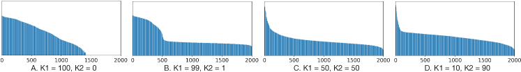
Figure 2: Modulating the posterior by controlling $K_{1}/K_{2}$. The topK only appproach leads to a collapsed posterior, which is overcome by $K_{2}$ randomization. Increasing $K_{2}$ encourages exploring less certain states, and consequently leads to an increasingly heavier tail.

Proposal Construction we consider the following:

$$q_{t}(i)=\frac{\phi(i,y_{t})}{2\sum_{j=1}^{N}\phi(j,y_{t})}+\frac{\left\lVert{\bm{e}}_{i}\right\rVert_{1}}{2\sum_{j=1}^{N}\left\lVert{\bm{e}}_{j}\right\rVert_{1}}$$ (34)

which consists of: (a). local weights (the first term is the normalized local emissions) where the intuitions is that states with larger local weights are more likely to be observed and (b). a global prior (the second term) where the intuition is that larger norms are usually associated with large dot products, and thus larger potentials. Note that there is no single fixed recipe of proposal construction since it is usually related to specific parameterization. For general structured models, we recommend considering utilizing any information that is potentially correlated with the actual summands, like the local and global weights we consider here.

Exploration-Exploitation Tradeoff It is important to note that gradients only pass through the top $K_{1}$ indices $\Omega_{t}^{K_{1}}$ and tail samples $\Omega_{t}^{K_{2}}$ during training. This means that increasing $K_{1}$ leads to exploiting states that are already confident enough while increasing $K_{2}$ leads to exploring less confident states. So the ratio $K_{1}/K_{2}$ also represents an exploration-exploitation tradeoff when searching for meaningful posterior structures. We will further see its effect in the experiments.

5 Experiments

We first evaluate the estimation error of individual RDP algorithms for three unit cases, namely when the underlying distributions are long-tail, intermediate level, or dense. Then we evaluate RDP for training the structured VAE.

5.1 Evaluation of RDP Algorithms

Experimental Setting We evaluate the mean square error (MSE) for the estimation of linear-chain log partition (Alg. 1), hypertree log partition (Alg. 2), and linear-chain entropy (Alg. 3) on the three types of distributions. We simulate the distributions by controlling their entropy: the smaller the entropy, the more long-tailed the underlying distribution is. We set $N$, the number of states, to be 2,000 and 10,000, which is orders of magnitudes larger than previous work (Wiseman et al., 2018; Yang et al., 2021). We run RDPs 100 times and calculate their MSE against the exact results from the full DP. For all estimators, we set $K_{2}=1$ and $K_{1}=K-1$, and control $K$ to be [1, 10, 20] percent of $N$. Also note that $K$ is independent of $N$ and we recommend adjusting it according to the computation budget. For linear-chains, we use the proposal discussed in Eq. 34. For hypertrees, we use a uniform proposal.

Comparison Models Since there is only a handful of methods that apply to this range of structures and inference, we choose topK summation (Sun et al., 2019) as our baseline. This method was originally developed for linear-chain partition function approximation, and can be viewed as setting $K_{2}=0$ in our case (topK summation only, no sample). This method is also used in Correia et al. (2020), however, they only consider sparse underlying distributions. It is important to differentiate between long-tailed and sparse distributions. While in both cases head elements consume a large portion of the probability mass, sparse means that tail elements have no probability while long-tailed means that tail elements have non-negligible probability. This entails that the topK approach (Sun et al., 2019; Correia et al., 2020) may significantly underestimate the partition function and entropy.

Table 5: Negative Log Likelihood comparison.

	Dev NLL	Test NLL
Full-100	39.64 $\pm$ 0.06	39.71 $\pm$ 0.07
TopK-100	39.71 $\pm$ 0.13	39.76 $\pm$ 0.11
RDP-100 (ours)	39.59 $\pm$ 0.10	39.59 $\pm$ 0.08
TopK-2000 (ours)	39.81 $\pm$ 0.30	39.84 $\pm$ 0.31
RDP-2000 (ours)	39.47 $\pm$ 0.11	39.48 $\pm$ 0.14

Results Table 2 shows the MSE results. Our method outperforms the topK baseline on all distributions with significantly less memory budgets. We highlight two important observations: (1) since TopK summation requires sparsity, it consistently underestimates the partition and entropy, particularly on dense distributions, while RDP does not have this limitation; and (2) by choosing only 1 percent of the full index, we are able to outperform TopK summation in many cases and obtain decent estimates.

Table 3 further shows how the computation budget of the randomized Forward algorithm can be used to control the bias-variance tradeoff. As can be seen, By increasing the computation budget $K$ (which is still smaller than full size), we are able to simultaneously reduce bias and variance. Table 4 shows different proposals influence the randomized Forward algorithm. We observe that a correlated proposal (as introduced in Eq. 34) indeed improves estimates of the randomized Forward. In general, scaled models typically require certain types of decomposition (see examples in Chiu et al. (2021) and Yang et al. (2021)) and proposals are closely related to a specific parametrization. For general structures, one can follow the local-global principle to construct proposals, or retreat to a uniform proposal.

5.2 Evaluation of the Structured VAE

We now use RDP to scale the latent space of the structured VAE. This experiment primarily tests the performance of the randomized Gumbel backward sampling algorithm (Alg. 4), which is used as a reparameterized gradient estimator for training the VAE.

Experimental Setting We use an LSTM with 256 dimensional hidden states for the generative model. For the inference model, we use a pretrained GPT2 (base size) to show our method’s compatibility with pretrained language models. We follow Fu et al. (2020) and use the MSCOCO dataset and reuse their processed data for simplicity. Our setting scales the original Gumbel-CRF paper (Fu et al., 2020). Specifically, we set $N=[100,2,000]$. With $N=100$ we can perform full DP which still gives biased gradients due to the continuous relaxation. With $N=2,000$, full DP gives memory overflow on a 16G GPU, so we only compare to the TopK approach. We use $K_{1}=K_{2}=10\%N$. We follow standard practice and report negative log likelihood estimated by importance sampling (Kim et al., 2019).

Results Table 5 shows the performance of Latent Variable Model training with varying $N$ size. We observe that RDP outperforms the baselines for both $N=100$ and $N=2,000$, which demonstrates its effectiveness for training VAEs. Furthermore, the overall NLL decreases as $N$ increases from 100 to 2,000, which underscores the advantage of scaling. We further show that the ratio of $K_{1}/K_{2}$ can be used for modulating the posterior and prevent posterior collapse. Specifically, we draw the frequency of states of the aggregated posterior. Recall that the aggregated posterior is obtained by sampling the latent states from the inference network for all training instances, then calculating the overall frequency (Mathieu et al., 2019). Figure 2 shows that topK summation leads to the posterior collapse as there exist multiple inactive states (frequency = 0). Here it is important to note that gradients only pass through the top $K_{1}$ indices $\Omega_{t}^{K_{1}}$ and tail samples $\Omega_{t}^{K_{2}}$ during training. This means that increasing $K_{1}$ leads to exploiting states that are already confident enough during training, while increasing $K_{2}$ leads to exploring less confident states, which consequently leads to increased tail frequency of the aggregated posterior (after convergence).

6 Conclusion

This work proposes the randomized sum-product algorithms for scaling structured models to tens of thousands of latent states. Our method is widely applicable to classical DP-based inference and different graph structures. Our methods reduce computation complexity by orders of magnitude compared to existing alternatives and is compatible with automatic differentiation and modern neural networks. We hope this method will open new possibilities of large-scale deep structured prediction models.

Appendix A Biasedness Analysis of Randomized Forward

In this section, we discuss the unbiasedness and variance of the Randomized Forward algorithm. We first show that Randomized Forward gives an unbiased estimator of the partition function.

Theorem A.1 (Unbiasedness).

For all $t\in[1,2,...,T]$, the sampled sum $\hat{\alpha}_{t}$ (Eq. 17) is an unbiased estimator of the forward variable $\alpha_{t}$. The final sampled sum $\hat{Z}$ is an unbiased estimator of the partition function $Z$.

Proof.

By the Second Principle of Mathematical Induction. Assume initialization $\alpha_{1}(i)=\phi(x_{1},i)$. Firstly at $t=2$, for all $i$, we have:

$$\mathbb{E}_{q_{1}}[\hat{\alpha}_{2}(i)]=\sum_{j=1}^{K_{1}}\alpha_{1}(\sigma_{1,j})\Phi(\sigma_{1,j},i)\phi(x_{2},i)+\frac{1}{K_{2}}\underbrace{\sum_{j=1}^{K_{2}}\mathbb{E}_{q_{1}}\bigg{[}\frac{\tilde{Z}_{1}}{\tilde{q}_{1}(\delta_{1,j})}\alpha_{1}(\delta_{1,j})\Phi(\delta_{1,j})\phi(x_{2},i)}_{=A}\bigg{]}$$ (35)

where the second term can be expanded as a masked summation with the index rearranged from $\sigma_{2,K_{1}+1}$ to $\sigma_{2,N}$:

$$A =\sum_{j=1}^{K_{2}}\mathbb{E}_{q_{1}}\bigg{[}\frac{\tilde{Z}_{1}}{\tilde{q}_{1}(\delta_{1,j})}\alpha_{1}(\delta_{1,j})\Phi(\delta_{1,j})\phi(x_{2},i)\bigg{]}$$ (36)

$$=\sum_{k=1}^{K_{2}}\sum_{j=K_{1}+1}^{N}\mathbb{E}_{q_{1}}\bigg{[}\frac{1}{q_{1}(\delta_{1,k})}\mathbbm{1}(\delta_{1,k}=j)\alpha_{1}(\sigma_{1,j})\Phi(\sigma_{1,j})\phi(x_{2},i)\bigg{]}$$ (37)

$$=\sum_{k=1}^{K_{2}}\sum_{j=K_{1}+1}^{N}\underbrace{\mathbb{E}_{q_{1}}\bigg{[}\frac{1}{q_{1}(\delta_{1,k})}\mathbbm{1}(\delta_{1,k}=j)\bigg{]}}_{=1}\alpha_{1}(\sigma_{1,j})\Phi(\sigma_{1,j})\phi(x_{2},i)$$ (38)

$$=K_{2}\sum_{j=K_{1}+1}^{N}\alpha_{1}(\sigma_{1,j})\Phi(\sigma_{1,j})\phi(x_{2},i)$$ (39)

Notice how we re-index the sum. Now put it back to Eq. 35 to get:

$$\mathbb{E}_{q_{1}}[\hat{\alpha}_{2}(i)] =\sum_{j=1}^{K_{1}}\alpha_{1}(\sigma_{1,j})\Phi(\sigma_{1,j},i)\phi(x_{2},i)+\frac{1}{K_{2}}\cdot K_{2}\sum_{j=K_{1}+1}^{N}\alpha_{1}(\sigma_{1,j})\Phi(\sigma_{1,j})\phi(x_{2},i)$$ (40)

$$=\sum_{j=1}^{N}\alpha_{1}(\sigma_{1,j})\Phi(\sigma_{,j},i)\phi(x_{2},i)$$ (41)

$$=\sum_{j=1}^{N}\alpha_{1}(j)\Phi(j,i)\phi(x_{2},i)$$ (42)

$$=\alpha_{2}(i)$$ (43)

This verifies the induction foundation that $\mathbb{E}_{q_{1}}[\hat{\alpha}_{2}(i)]=\alpha_{2}(i)$ for all $i$.

Now assume for all time index up to $t$ we have:

$$\forall i,\mathbb{E}_{q_{1:t-1}}[\hat{\alpha}_{t}(i)]=\alpha_{t}(i)$$ (44)

Consider $t+1$, we have:

$$\mathbb{E}_{1:q_{t}}[\hat{\alpha}_{t+1}(i)] =\sum_{j=1}^{K_{1}}\mathbb{E}_{q_{1:{t-1}}}\big{[}\hat{\alpha}_{t}(\sigma_{t,j})\big{]}\Phi(\sigma_{t,j},i)\phi(x_{t+1},i)$$ (45)

$$\quad\quad+\frac{1}{K_{2}}\sum_{j=1}^{K_{2}}\mathbb{E}_{q_{1:t-1}}\big{[}\hat{\alpha}_{t}(\delta_{t,j})\big{]}\cdot\mathbb{E}_{q_{t}}\big{[}\frac{\tilde{Z}_{t}}{\tilde{q}_{t}(\delta_{t,j})}\Phi(\delta_{t,j})\phi(x_{t+1},i)]\big{]}$$ (46)

$$=\sum_{j=1}^{K_{1}}\alpha_{t}(\sigma_{t,j})\Phi(\sigma_{t,j},i)\phi(x_{t+1},i)$$ (47)

$$\quad\quad+\frac{1}{K_{2}}\underbrace{\sum_{j=1}^{K_{2}}\alpha_{t}(\sigma_{t,j})\cdot\mathbb{E}_{q_{t}}\big{[}\frac{\tilde{Z}_{t}}{\tilde{q}_{t}(\delta_{t,j})}\Phi(\delta_{t,j})\phi(x_{t+1},i)]\big{]}}_{=A^{\prime}}$$ (48)

Note how we decompose the expectation by using the independence: $q_{1:t}=q_{1:t-1}\cdot q_{t}$ With a similar masked summation trick as $A$, we have:

$$A^{\prime}=K_{2}\sum_{j=K_{1}+1}^{N}\alpha_{t}(\sigma_{t,j})\Phi(\sigma_{t,j},i)\phi(x_{t+1},i)$$ (49)

This gives us:

$$\mathbb{E}_{1:q_{t}}[\hat{\alpha}_{t+1}(i)] =\sum_{j=1}^{K_{1}}\alpha_{t}(\sigma_{t,j})\Phi(\sigma_{t,j},i)\phi(x_{t+1},i)+\frac{1}{K_{2}}\cdot K_{2}\sum_{j=K_{1}+1}^{N}\alpha_{t}(\sigma_{t,j})\Phi(\sigma_{t,j},i)\phi(x_{t+1},i)$$ (50)

$$=\sum_{j=1}^{N}\alpha_{t}(\sigma_{t,j})\Phi(\sigma_{t,j},i)\phi(x_{t+1},i)$$ (51)

$$=\sum_{j=1}^{N}\alpha_{t}(j)\Phi(j,i)\phi(x_{t+1},i)$$ (52)

$$=\alpha_{t+1}(i)$$ (53)

Thus showing $\hat{\alpha}_{t+1}$ is also an unbiased estimator for $\alpha_{t+1}$ at each step $t+1$. Setting $t=T$, the last step, gives us $\mathbb{E}[\hat{Z}]=Z$ (details similar to the above). ∎

Corollary A.2.

When we change the (sum, product) semiring to the (log-sum-exp, sum) semiring, the expectation of the estimator will become a lower bound of $\log\alpha_{t}$ and $\log Z$.

Proof.

Denote $l_{t}(i)=\log\alpha_{t}(i)$ and $\Omega$ the set of sampled indices where $|\Omega|=K_{2}$. For simplicity, we omit the top $K_{1}$ summation and only show the summation of the sample. Cases where $t>2$ can be derived similarly as following:

$$\hat{l}_{2}(i) =\log\sum_{j\in\Omega}\exp(l_{1}(j)+\log\Phi(j,i)+\log\phi(x_{t},i))-\log K_{2}$$ (54)

$$\mathbb{E}[\hat{l}_{2}(i)] =\mathbb{E}\bigg{[}\log\sum_{j\in\Omega}\exp(l_{1}(j)+\log\Phi(j,i)+\log\phi(x_{t},i))\bigg{]}-\log K_{2}$$ (55)

$$\leq\log\mathbb{E}\bigg{[}\sum_{j\in\Omega}\exp(l_{1}(j)+\log\Phi(j,i)+\log\phi(x_{t},i))\bigg{]}-\log K_{2}$$ (56)

$$=\log K_{2}-\log K_{2}+\log\sum_{j\in\Omega}\exp(l_{1}(j)+\log\Phi(j,i)+\log\phi(x_{t},i))$$ (57)

$$=l_{2}(i)$$ (58)

where Eq. 56 comes from Jensen’s inequality. Then by induction one can show at everystep, we have $\mathbb{E}[\hat{l}_{t}(i)]\leq l_{t}(i)$. ∎

Although implementation in the log space makes the estimate biased, it reduces the variance exponentially in a rather trivial way. It also provides numerical stability. So, in practice we use it for training.

Appendix B Variance Analysis of Randomized Forward

Now we analyze variance. We start with the estimator $a_{\delta}/q_{\delta}$, $\delta\sim\text{Categorical}\{q_{K_{1}+1},...q_{K_{N}}\}$ in Eq. 4. Firstly, this is an unbiased estimator of the tail sum:

$$\mathbb{E}[a_{\delta}/q_{\delta}]=\sum_{i=K_{1}+1}^{N}a_{i}$$ (59)

We have the folling variance arguments:

Theorem B.1 (Variance of the tail estimator).

$$\mathbb{V}[a_{\delta}/q_{\delta}] =\sum_{i=K_{1}+1}^{N}a_{i}^{2}/q_{i}-(\sum_{i=K_{1}+1}^{N}a_{i})^{2}$$ (60)

$$=S_{K_{1}}^{2}(\sum_{i=K_{1}+1}^{N}\epsilon_{i}^{2}/q_{i}+2\epsilon_{i})$$ (61)

where

$$S_{K_{1}}=\sum_{i=K_{1}+1}^{N}a_{i}\quad\quad\quad\quad\epsilon_{i}=a_{i}/S_{K_{1}}-q_{i}$$ (62)

which says the variance is:

• quadratic to the tail sum $S_{K_{1}}$, which will can be reduced by increasing $K_{1}$ as the effect of Rao-Blackwellization.

• approximately quadratic to the gap $\epsilon_{i}$, as the differences between the proposal $q_{i}$ and the oracle $a_{i}/S_{K_{1}}$, which can be reduced by choosing a correlated proposal as the effect of importance sampling.

Optimal zero variance is achieved on

$$q_{i}^{*}=a_{i}/S_{K_{1}}$$ (63)

Proof.

The variance is then:

$$\mathbb{V}[a_{\delta}/q_{\delta}]=\mathbb{E}[(a_{\delta}/q_{\delta})^{2}]-\mathbb{E}[a_{\delta}/q_{\delta}]^{2}$$ (64)

where the first term is the second moment:

$$(a_{\delta}/q_{\delta})^{2} =(\sum_{i=K_{1}+1}^{N}a_{i}\mathbbm{1}[\delta=i]/q_{i})^{2}$$ (65)

$$=\sum_{i=K_{1}+1}^{N}a_{i}^{2}\mathbbm{1}[\delta=i]/q_{i}^{2}+\underbrace{2\sum_{i=K_{1}+1}^{N}\sum_{j=K_{1}+1}^{N}\frac{a_{i}a_{j}\mathbbm{1}[\delta=i]\mathbbm{1}[\delta=j]}{q_{i}q_{j}}}_{=0}$$ (66)

$$=\sum_{i=K_{1}+1}^{N}a_{i}^{2}\mathbbm{1}[\delta=i]/q_{i}^{2}$$ (67)

taking the expection of it we get:

$$\mathbb{E}[(a_{\delta}/q_{\delta})^{2}] =\mathbb{E}[\sum_{i=K_{1}+1}^{N}a_{i}^{2}\mathbbm{1}[\delta=i]/q_{i}^{2}]$$ (68)

$$=\sum_{i=K_{1}+1}^{N}a_{i}^{2}/q_{i}$$ (69)

Plug this back, variance is:

$$\mathbb{V}[a_{\delta}/q_{\delta}]=\sum_{i=K_{1}+1}^{N}a_{i}^{2}/q_{i}-(\sum_{i=K_{1}+1}^{N}a_{i})^{2}$$ (70)

To get the optimal proposal, we solve the constrained optimization problem:

$$\min_{q_{i}}\sum_{i=K_{1}+1}^{N}a_{i}^{2}/q_{i}-(\sum_{i=K_{1}+1}^{N}a_{i})^{2}$$ (71)

$$s.t.\sum_{i=K_{1}+1}^{N}q_{i}=1$$ (72)

By solving the corresponding Lagrangian equation system (omitted here), we get the optimal value achieved at:

$$q_{i}^{*}=\frac{a_{i}}{\sum_{i=K_{1}+1}^{N}a_{i}} \sum_{i=K_{1}+1}^{N}a_{i}^{2}/q_{i}^{*}-(\sum_{i=K_{1}+1}^{N}a_{i})^{2}=0$$ (73)

This says zero variance is achieved by a proposal equal to the normalized summands.

Then define the gap between the proposal and the normalized summands as:

$$\epsilon_{i}=\frac{a_{i}}{S_{K_{1}}}-q_{i}$$ (74)

Plug this to the variance expression we get:

$$\mathbb{V}[a_{\delta}/q_{\delta}]=S_{K_{1}}^{2}(\sum_{i=K_{1}+1}^{N}\epsilon_{i}^{2}/q_{i}+2\epsilon_{i})$$ (75)

∎

Corollary B.2.

When increasing the sample size to $K_{2}$, the variance will reduce to

$$\mathbb{V}[\frac{1}{K_{2}}\sum_{j=1}^{N}\frac{a_{\delta_{j}}}{q_{\delta_{j}}}]=\frac{1}{K_{2}}S_{K_{1}}^{2}(\sum_{i=K_{1}+1}^{N}\epsilon_{i}^{2}/q_{i}+2\epsilon_{i})$$ (76)

Now we consider the variance of the Sampled Forward algorithm. An exact computation would give complicated results. For simplification, we give an asymptotic argument with regard to Rao-Blackwellization and importance sampling:

Theorem B.3 (Single Step Asymptotic Variance of Sampled Forward).

At each step, the alpha varible estimator has the following asymptotic variance:

$$\mathbb{V}[\hat{\alpha}_{t}(i)]=O\Big{(}\frac{1}{K_{2}}\alpha^{2}_{t,K_{1}}(i)\cdot\epsilon^{2}_{t}(i)\Big{)}$$ (77)

where:

• $\alpha_{t+1,K_{1}}(i)=\sum_{j=K_{1}+1}^{N}\tilde{\alpha}_{t}(j,i)=\sum_{j=K_{1}+1}^{N}\sqrt{\mathbb{E}_{q_{1:t-1}}[\hat{\alpha}^{2}_{t}(j)]}\Phi(j,i)\phi(x_{t},i)$ is a tail sum after the top $K_{1}$ summands. This term will reduce if we increase $K_{1}$, as an instance of Rao-Blackwellization.

• $\epsilon^{2}_{t}(i)=\sum_{j=K_{1}+1}^{N}\epsilon^{2}_{t-1}(j,i)/q_{t-1}(j)$ and $\epsilon_{t-1}(j,i)$ is the difference between the proposal $q_{t-1}(j)$ and the oracle proposal. This term will reduce if the proposal is more correlated to the oracle, as an instance of Importance Sampling.

Proof.

We start with a simple setting where $K_{2}=1$. At step $t+1$ we have the following variance recursion:

$$\mathbb{E}_{q_{1:t}}[\hat{\alpha}^{2}_{t+1}(i)]=\sum_{j=K_{1}+1}^{N}\frac{\Phi^{2}(j,i)\phi^{2}(x_{t+1},i)}{q_{t}(j)}\cdot\mathbb{E}_{q_{1:t-1}}[\hat{\alpha}_{t}^{2}(j)]$$ (78)

This is derived by plugging estimator 17 to the variance Eq. 60 we have just derived. Denote:

$$\alpha_{t+1,K_{1}}(i)=\sum_{j=K_{1}+1}^{N}\tilde{\alpha}_{t}(j,i)=\sum_{j=K_{1}+1}^{N}\sqrt{\mathbb{E}_{q_{1:t-1}}[\hat{\alpha}^{2}_{t}(j)]}\Phi(j,i)\phi(x_{t+1},i)$$ (79)

Then we have

$$\mathbb{V}_{q_{1:t}}[\hat{\alpha}_{t+1}(i)]=\alpha^{2}_{t+1,K_{1}}(i)\big{(}\sum_{j=K_{1}+1}^{N}\frac{\epsilon_{t}^{2}(j,i)}{q_{t}(i)}+2\epsilon_{t}(j,i)\big{)}$$ (80)

where $\epsilon_{t}(j,i)$ is the differences between the proposal and the normalized exact summands at step $t$ state $i$:

$$\epsilon_{t}(j,i)=\frac{\tilde{\alpha}_{t}(j,i)}{\sum_{j=K_{1}=1}^{N}\tilde{\alpha}_{t}(j,i)}-q_{t}(j)$$ (81)

Dropping out the first order errors and increasing the number of sample to $K_{2}$, we have the asymptotics:

$$\mathbb{V}[\hat{\alpha}_{t}(i)]=O\Big{(}\frac{1}{K_{2}}\alpha^{2}_{t,K_{1}}(i)\cdot\epsilon^{2}_{t}(i)\Big{)}$$ (82)

∎

Theorem B.4 (Asymptotic Variance of Sampled Forward Partition Estimation).

The alpha variable estimators has the following asymptotic variance recurrsion:

$$\mathbb{V}[\hat{\alpha}_{t+1}(i)]=O(\frac{1}{K_{2}}\cdot\phi_{t,K_{1}}^{2}\cdot\epsilon_{t,K_{1}}^{2}\cdot\mathbb{V}[\hat{\alpha}_{t}])$$ (83)

Compared with Eq. 77, this expression:

• Uses the product of the factors $\phi_{t,K_{1}}$ (a function of the sum-prod of the factor at step $t$) and the previous step variance $\mathbb{V}[\hat{\alpha}_{t}]$ to substitute the $\alpha_{t,K_{1}}$ in equation 77. Again, this term will decrease with a larger $K_{1}$ (Rao-Blackwellization).

• $\epsilon^{2}_{t,K_{1}}(i)=\sum_{j=K_{1}+1}^{N}\epsilon^{2}_{t-1}(j,i)/q_{t-1}(j)$ and $\epsilon_{t-1}(j,i)$ is the difference between the proposal $q_{t-1}(j)$ and the oracle proposal. This term will reduce if the proposal is more correlated to the oracle, as an instance of Importance Sampling (same as Eq. 77).

Consequently, the partition function has the following asymptotic variance:

$$\mathbb{V}[\hat{Z}]=O(\prod_{t=1}^{T}\frac{1}{K_{2}}\cdot\phi_{t,K_{1}}^{2}\cdot\epsilon_{t,K_{1}}^{2})$$ (84)

When implemented in the log space, the variance is trivially reduced exponentially:

$$\mathbb{V}[\log\hat{Z}]=O(\sum_{t=1}^{T}\log\frac{1}{K_{2}}+2\log\phi_{t,K_{1}}+2\log\epsilon_{t,K_{1}})$$ (85)

Proof.

Firstly for simplcity we assume $K_{1}=0$ and $K_{2}=1$. The the estimator variance is:

$$\mathbb{V}[\hat{\alpha}_{t+1}(i)] =\mathbb{E}_{q_{1:t}}[\hat{\alpha}_{t+1}^{2}(i)]-\alpha_{t+1}^{2}(i)$$ (86)

$$=\mathbb{E}_{q_{1:t-1}}\bigg{[}\sum_{j=1}^{N}\frac{\hat{\alpha}_{t}^{2}(j)\Phi^{2}(j,i)\phi^{2}(x_{t},i)}{q_{t}(j)}\cdot\frac{\alpha_{t}^{2}(j)}{\alpha_{t}^{2}(j)}\bigg{]}-\alpha_{t+1}^{2}(i)$$ (87)

Recall:

$$\alpha_{t+1}(i)=\sum_{j=1}^{N}\alpha_{t}(j)\phi(j,i)\phi(x_{t},i)$$ (88)

Let:

$$\epsilon_{t}(j,i)=\underbrace{\frac{\alpha_{t}(j)\phi(j,i)\phi(x_{t},i)}{\alpha_{t+1}(i)}}_{=q(z_{t}=j|z_{t+1}=i)}-q_{t}(j)$$ (89)

Then:

$$\mathbb{V}[\hat{\alpha}_{t+1}(i)] =\mathbb{E}_{q_{1:t-1}}\bigg{[}\sum_{j=1}^{N}\alpha_{t+1}^{2}(i)\big{(}\frac{\epsilon_{t}^{2}(j,i)}{q_{t}(j)}+2\epsilon_{t}(j,i)+q_{t}(j)\big{)}\frac{\hat{\alpha}_{t}^{2}(j)}{\alpha_{t}^{2}(j)}\bigg{]}-\alpha_{t+1}^{2}(i)$$ (90)

$$=\alpha_{t+1}^{2}(i)\bigg{(}\sum_{j=1}^{N}\big{(}\frac{\mathbb{E}_{q_{1:t-1}}[\hat{\alpha}_{t}^{2}(j)]}{\alpha_{t}^{2}(j)}q_{t}(j)\big{)}+\sum_{j=1}^{N}\big{(}\frac{\epsilon_{t}^{2}(j,i)}{q_{t}(j)}+2\epsilon_{t}(j,i)\big{)}\frac{\mathbb{E}_{q_{1:t-1}}[\hat{\alpha}_{t}^{2}(j)]}{\alpha_{t}^{2}(j)}\bigg{)}$$ (91)

$$\quad-\alpha_{t+1}^{2}(i)$$ (92)

Note that there exist $J_{t}$ such that:

$$\frac{\mathbb{E}_{q_{1:t-1}}[\hat{\alpha}_{t}^{2}(j)]}{\alpha_{t}^{2}(j)}<=J_{t}$$ (93)

This is because of the bounded gap of the Jensen’s inequality. Also recall:

$$\sum_{j=1}^{N}q_{t}(j)=1$$ (94)

So we get:

$$\mathbb{V}[\hat{\alpha}_{t+1}(i)] <=\alpha_{t+1}^{2}(i)\bigg{(}J_{t}-1+\sum_{j=1}^{N}\big{(}\frac{\epsilon_{t}^{2}(j,i)}{q_{t}(j)}+2\epsilon_{t}(j,i)\big{)}\cdot\big{(}\frac{\mathbb{V}[\hat{\alpha}_{t}(j)]}{\alpha_{t}^{2}(j)}-1\big{)}\bigg{)}$$ (95)

$$=\alpha_{t+1}^{2}(i)\bigg{(}J_{t}-1-\sum_{j=1}^{N}\big{(}\frac{\epsilon_{t}^{2}(j,i)}{q_{t}(j)}+2\epsilon_{t}(j,i)\big{)}\bigg{)}$$ (96)

$$\quad+\alpha_{t+1}^{2}(i)\bigg{(}\sum_{j=1}^{N}\big{(}\frac{\epsilon_{t}^{2}(j,i)}{q_{t}(j)}+2\epsilon_{t}(j,i)\big{)}\cdot\big{(}\frac{\mathbb{V}[\hat{\alpha}_{t}(j)]}{\alpha_{t}^{2}(j)}\big{)}\bigg{)}$$ (97)

empirically $J_{t}$ is not the dominate source of variance (but could be in the worst case, depending on the tightness of Jensen’s inequality). We focus on the second term:

$$\mathbb{V}[\hat{\alpha}_{t+1}(i)] =O\bigg{(}\alpha_{t+1}^{2}(i)\bigg{(}\sum_{j=1}^{N}\big{(}\frac{\epsilon_{t}^{2}(j,i)}{q_{t}(j)}+2\epsilon_{t}(j,i)\big{)}\cdot\big{(}\frac{\mathbb{V}[\hat{\alpha}_{t}(j)]}{\alpha_{t}^{2}(j)}\big{)}\bigg{)}$$ (98)

$$=O\bigg{(}\Big{(}\sum_{j=1}^{N}\alpha_{t}(j)\underbrace{\Phi(j,i)\phi(x_{t},j)}_{O(\phi_{t}^{2})}\Big{)}^{2}\cdot\Big{(}\underbrace{\sum_{j=1}^{N}\big{(}\frac{\epsilon_{t}^{2}(j,i)}{q_{t}(j)}+2\epsilon_{t}(j,i)\big{)}}_{O(\epsilon_{t}^{2})}\cdot\frac{1}{\alpha_{t}^{2}(j)}\cdot\underbrace{\mathbb{V}[\hat{\alpha}_{t}(j)]}_{O(\mathbb{V}[\alpha_{t}])}\Big{)}\bigg{)}$$ (99)

$$=O(\phi_{t}^{2}\cdot\epsilon_{t}^{2}\cdot\mathbb{V}[\alpha_{t}])$$ (100)

Note that a lot of higher-order sum-products are simplified here. Adding top $K_{1}$ summation and increasing the sample size to $K_{2}$ leads to variance reduction as:

$$\mathbb{V}[\hat{\alpha}_{t+1}(i)] =O(\frac{1}{K_{2}}\cdot\phi_{t,K_{1}}^{2}\cdot\epsilon_{t,K_{1}}^{2}\cdot\mathbb{V}[\alpha_{t}])$$ (101)

Recursively expand this equation we get:

$$\mathbb{V}[\hat{Z}]=O(\prod_{t=1}^{T}\frac{1}{K_{2}}\cdot\phi_{t,K_{1}}^{2}\cdot\epsilon_{t,K_{1}}^{2})$$ (102)

Chaning the implementation to the log space we reduce the variance exponentially:

$$\mathbb{V}[\log\hat{Z}]=O(\sum_{t=1}^{T}\log\frac{1}{K_{2}}+2\log\phi_{t,K_{1}}+2\log\epsilon_{t,K_{1}})$$ (103)

∎

References

- Ammar et al. (2014) Ammar, W., Dyer, C., and Smith, N. A. Conditional random field autoencoders for unsupervised structured prediction. In Advances in Neural Information Processing Systems, pp. 3311–3319, 2014.
- Beatson & Adams (2019) Beatson, A. and Adams, R. P. Efficient optimization of loops and limits with randomized telescoping sums. In Chaudhuri, K. and Salakhutdinov, R. (eds.), Proceedings of the 36th International Conference on Machine Learning, volume 97 of Proceedings of Machine Learning Research, pp. 534–543. PMLR, 09–15 Jun 2019. URL https://proceedings.mlr.press/v97/beatson19a.html.
- Blunsom & Cohn (2010) Blunsom, P. and Cohn, T. Inducing synchronous grammars with slice sampling. In Human Language Technologies: The 2010 Annual Conference of the North American Chapter of the Association for Computational Linguistics, pp. 238–241, Los Angeles, California, June 2010. Association for Computational Linguistics. URL https://aclanthology.org/N10-1028.
- Bouchard-côté et al. (2009) Bouchard-côté, A., Petrov, S., and Klein, D. Randomized pruning: Efficiently calculating expectations in large dynamic programs. In Bengio, Y., Schuurmans, D., Lafferty, J., Williams, C., and Culotta, A. (eds.), Advances in Neural Information Processing Systems, volume 22. Curran Associates, Inc., 2009. URL https://proceedings.neurips.cc/paper/2009/file/e515df0d202ae52fcebb14295743063b-Paper.pdf.
- Chiu & Rush (2020) Chiu, J. and Rush, A. M. Scaling hidden markov language models. In Proceedings of the 2020 Conference on Empirical Methods in Natural Language Processing (EMNLP), pp. 1341–1349, 2020.
- Chiu et al. (2021) Chiu, J. T., Deng, Y., and Rush, A. M. Low-rank constraints for fast inference in structured models. In Thirty-Fifth Conference on Neural Information Processing Systems, 2021. URL https://openreview.net/forum?id=Mcldz4OJ6QB.
- Correia et al. (2020) Correia, G., Niculae, V., Aziz, W., and Martins, A. Efficient marginalization of discrete and structured latent variables via sparsity. Advances in Neural Information Processing Systems, 33, 2020.
- Corro & Titov (2018) Corro, C. and Titov, I. Differentiable perturb-and-parse: Semi-supervised parsing with a structured variational autoencoder. arXiv preprint arXiv:1807.09875, 2018.
- Eisner (2016) Eisner, J. Inside-outside and forward-backward algorithms are just backprop (tutorial paper). In Proceedings of the Workshop on Structured Prediction for NLP, pp. 1–17, Austin, TX, November 2016. Association for Computational Linguistics. doi: 10.18653/v1/W16-5901. URL https://aclanthology.org/W16-5901.
- Fu et al. (2020) Fu, Y., Tan, C., Bi, B., Chen, M., Feng, Y., and Rush, A. M. Latent template induction with gumbel-crf. In NeurIPS, 2020.
- Halko et al. (2011) Halko, N., Martinsson, P. G., and Tropp, J. A. Finding structure with randomness: Probabilistic algorithms for constructing approximate matrix decompositions. SIAM Review, 53(2):217–288, 2011. doi: 10.1137/090771806. URL https://doi.org/10.1137/090771806.
- Jeong et al. (2009) Jeong, M., Lin, C.-Y., and Lee, G. G. Efficient inference of crfs for large-scale natural language data. In Proceedings of the ACL-IJCNLP 2009 Conference Short Papers, pp. 281–284, 2009.
- Kim et al. (2019) Kim, Y., Rush, A. M., Yu, L., Kuncoro, A., Dyer, C., and Melis, G. Unsupervised recurrent neural network grammars. In Proceedings of the 2019 Conference of the North American Chapter of the Association for Computational Linguistics: Human Language Technologies, Volume 1 (Long and Short Papers), pp. 1105–1117, 2019.
- Klein & Manning (2003) Klein, D. and Manning, C. D. A* parsing: Fast exact viterbi parse selection. In Proceedings of the 2003 Human Language Technology Conference of the North American Chapter of the Association for Computational Linguistics, pp. 119–126, 2003.
- Lavergne et al. (2010) Lavergne, T., Cappé, O., and Yvon, F. Practical very large scale crfs. In Proceedings of the 48th Annual Meeting of the Association for Computational Linguistics, pp. 504–513, 2010.
- Li et al. (2020) Li, C., Gao, X., Li, Y., Peng, B., Li, X., Zhang, Y., and Gao, J. Optimus: Organizing sentences via pre-trained modeling of a latent space. In Proceedings of the 2020 Conference on Empirical Methods in Natural Language Processing (EMNLP), pp. 4678–4699, 2020.
- Li & Rush (2020) Li, X. L. and Rush, A. Posterior control of blackbox generation. In Proceedings of the 58th Annual Meeting of the Association for Computational Linguistics, pp. 2731–2743, Online, July 2020. Association for Computational Linguistics. doi: 10.18653/v1/2020.acl-main.243. URL https://aclanthology.org/2020.acl-main.243.
- Liu et al. (2019) Liu, R., Regier, J., Tripuraneni, N., Jordan, M., and Mcauliffe, J. Rao-blackwellized stochastic gradients for discrete distributions. In International Conference on Machine Learning, pp. 4023–4031. PMLR, 2019.
- Ma & Hovy (2016) Ma, X. and Hovy, E. End-to-end sequence labeling via bi-directional LSTM-CNNs-CRF. In Proceedings of the 54th Annual Meeting of the Association for Computational Linguistics (Volume 1: Long Papers), pp. 1064–1074, Berlin, Germany, August 2016. Association for Computational Linguistics. doi: 10.18653/v1/P16-1101. URL https://aclanthology.org/P16-1101.
- Mahoney (2011) Mahoney, M. W. Randomized algorithms for matrices and data. Found. Trends Mach. Learn., 3(2):123–224, feb 2011. ISSN 1935-8237. doi: 10.1561/2200000035. URL https://doi.org/10.1561/2200000035.
- Martins et al. (2019) Martins, A. F. T., Mihaylova, T., Nangia, N., and Niculae, V. Latent structure models for natural language processing. In Proceedings of the 57th Annual Meeting of the Association for Computational Linguistics: Tutorial Abstracts, pp. 1–5, Florence, Italy, July 2019. Association for Computational Linguistics. doi: 10.18653/v1/P19-4001. URL https://aclanthology.org/P19-4001.
- Mathieu et al. (2019) Mathieu, E., Rainforth, T., Siddharth, N., and Teh, Y. W. Disentangling disentanglement in variational autoencoders. In International Conference on Machine Learning, pp. 4402–4412. PMLR, 2019.
- Mensch & Blondel (2018) Mensch, A. and Blondel, M. Differentiable dynamic programming for structured prediction and attention. In International Conference on Machine Learning, pp. 3462–3471. PMLR, 2018.
- Mohamed et al. (2020) Mohamed, S., Rosca, M., Figurnov, M., and Mnih, A. Monte carlo gradient estimation in machine learning. J. Mach. Learn. Res., 21(132):1–62, 2020.
- Oktay et al. (2020) Oktay, D., McGreivy, N., Aduol, J., Beatson, A., and Adams, R. P. Randomized automatic differentiation. In International Conference on Learning Representations, 2020.
- Paulus et al. (2020) Paulus, M. B., Choi, D., Tarlow, D., Krause, A., and Maddison, C. J. Gradient estimation with stochastic softmax tricks. arXiv preprint arXiv:2006.08063, 2020.
- Potapczynski et al. (2021) Potapczynski, A., Wu, L., Biderman, D., Pleiss, G., and Cunningham, J. P. Bias-free scalable gaussian processes via randomized truncations. In Meila, M. and Zhang, T. (eds.), Proceedings of the 38th International Conference on Machine Learning, volume 139 of Proceedings of Machine Learning Research, pp. 8609–8619. PMLR, 18–24 Jul 2021. URL https://proceedings.mlr.press/v139/potapczynski21a.html.
- Ranganath et al. (2014) Ranganath, R., Gerrish, S., and Blei, D. Black Box Variational Inference. In Kaski, S. and Corander, J. (eds.), Proceedings of the Seventeenth International Conference on Artificial Intelligence and Statistics, volume 33 of Proceedings of Machine Learning Research, pp. 814–822, Reykjavik, Iceland, 22–25 Apr 2014. PMLR. URL https://proceedings.mlr.press/v33/ranganath14.html.
- Rhodes et al. (2020) Rhodes, B., Xu, K., and Gutmann, M. U. Telescoping density-ratio estimation. In Larochelle, H., Ranzato, M., Hadsell, R., Balcan, M. F., and Lin, H. (eds.), Advances in Neural Information Processing Systems, volume 33, pp. 4905–4916. Curran Associates, Inc., 2020. URL https://proceedings.neurips.cc/paper/2020/file/33d3b157ddc0896addfb22fa2a519097-Paper.pdf.
- Rush (2020) Rush, A. M. Torch-struct: Deep structured prediction library. In Proceedings of the 58th Annual Meeting of the Association for Computational Linguistics: System Demonstrations, pp. 335–342, 2020.
- Sokolovska et al. (2010) Sokolovska, N., Lavergne, T., Cappé, O., and Yvon, F. Efficient learning of sparse conditional random fields for supervised sequence labeling. IEEE Journal of Selected Topics in Signal Processing, 4:953–964, 2010.
- Sun et al. (2019) Sun, Z., Li, Z., Wang, H., He, D., Lin, Z., and Deng, Z. Fast structured decoding for sequence models. Advances in Neural Information Processing Systems, 32:3016–3026, 2019.
- Sutton & McCallum (2006) Sutton, C. and McCallum, A. An introduction to conditional random fields for relational learning. Introduction to statistical relational learning, 2:93–128, 2006.
- Wainwright & Jordan (2008) Wainwright, M. J. and Jordan, M. I. Graphical models, exponential families, and variational inference. Now Publishers Inc, 2008.
- Wiseman et al. (2018) Wiseman, S., Shieber, S., and Rush, A. Learning neural templates for text generation. In Proceedings of the 2018 Conference on Empirical Methods in Natural Language Processing, pp. 3174–3187, Brussels, Belgium, October-November 2018. Association for Computational Linguistics. doi: 10.18653/v1/D18-1356. URL https://aclanthology.org/D18-1356.
- Yang et al. (2021) Yang, S., Zhao, Y., and Tu, K. Pcfgs can do better: Inducing probabilistic context-free grammars with many symbols. arXiv preprint arXiv:2104.13727, 2021.
- Zhang et al. (2020) Zhang, Y., Li, Z., and Zhang, M. Efficient second-order treecrf for neural dependency parsing. arXiv preprint arXiv:2005.00975, 2020.