Applications of the Frenet Frame to Electric Circuits

Abstract

The paper discusses the relationships between electrical quantities, such as voltages, currents, and frequency, and geometrical ones, namely curvature and torsion. The proposed approach is based on the Frenet frame utilized in differential geometry and provides a general framework for the definition of the time derivative of electrical quantities in stationary as well as transient conditions. As a byproduct, the proposed approach unifies and generalizes the time- and phasor-domain frameworks. Other noteworthy results are a new interpretation of the link between frequency and the time derivatives of voltage and current; and a definition of the rate of change of frequency that includes the novel concept of “torsional frequency.” Several numerical examples based on balanced, unbalanced, harmonically-distorted and transient voltages illustrate the findings of the paper.

I Notation

In this paper, scalars are indicated with normal font, e.g. $x$, whereas vectors are indicated in bold face, e.g. $\boldsymbol{x}=(x_{1},x_{2},x_{3})$. All vectors have order 3, unless otherwise indicated.

Scalars

• length of a curve

• time

• voltage magnitude

• angular frequency

• symmetric part of the geometric RoCoF

• voltage phase angle

• curvature

• torsional frequency

• symmetric part of the geometric frequency

• torsion

• magnitude of vector $\boldsymbol{\omega}$

Vectors

• null vector

• binormal vector of the Frenet frame

• $i$-th vector of an orthonormal basis

• current vector

• normal vector before normalization

• normal vector of the Frenet frame

• electric charge vector

• tangent vector of the Frenet frame

• voltage vector

• magnetic flux vector

• antisymmetric part of the geometric frequency

Derivatives

• derivative of a scalar/vector with respect to $t$

• derivative of a scalar/vector with respect to $s$

• time derivative operator applied to vector $\boldsymbol{x}$

II Introduction

II-A Motivation

The study and simulation of circuit dynamics has traditionally been approached using different frameworks. Stationary AC circuits are conveniently studied using quantities such as phasors and impedances; circuits with harmonic contents are studied using Fourier analysis or similar frequency-domain approaches; rotating machines and power electronic devices are often studied using Park and/or Clarke transforms; generic transients are studied using a time-domain analysis [1]. In this paper, we propose an approach based on differential geometry, more specifically on the Frenet frame [2]. This approach leads to the definition of a framework that admits, as special cases, the circuit analysis transformations mentioned above.

II-B Literature Review

Differential geometry finds applications in several fields of science and engineering. Some examples are the use of differential geometric properties, such as that of curvature, in image segmentation and three-dimensional object description [3], as well as in robotic control along geodesic paths [4]. Another relevant example are the utilities of the Frenet frame in the area of autonomous vehicle driving [5, 6]. Moreover, there is a number of applications that are based on the theory of geometric algebra, for example the use of quaternions in computer graphics and visualization [7, 8] and in the control of multi-agent networked systems [9].

The utilization of concepts of geometric algebra in circuit and power system analysis is limited. There is a group of works that elaborate on the concept of instantaneous power [10, 11, 12, 13, 14, 15] that provide an interpretation of the active and reactive power as the inner and cross (or wedge in the polyphase case) products, respectively, of voltage and currents. More recently, some studies, including [16, 17, 18, 19, 20], have attempted to extend the instantaneous power theory to a systematic study of electrical quantities or circuits in the framework of geometric algebra. In the same vein, but using a novel perspective, [21] makes an additional step by proposing to interpret voltages and currents as the time derivative of a multi-dimensional curve. This interpretation allows the definition of the “geometric frequency” as the result of an inner and an outer product.

In this work, we exploit differential geometry rather than geometric algebra. We are interested in the geometrical “meaning” of the time derivative of electrical quantities such as voltage, current and frequency. With this aim, the formulas obtained in the paper are deduced through the Frenet frame [2]. The importance in circuit analysis of the time derivatives of voltages and currents is apparent as they are required in the constitutive equations of capacitors and inductors. The relevance of the Rate of Change of Frequency (RoCoF), on the other hand, is due to the increasing penetration, in the electric grid all around the world, of renewable energy sources and the consequent shift from synchronous to non-synchronous generation. The RoCoF is, in turn, strictly related to the amount of available inertia in the system [22]. The ability to estimate accurately the RoCoF is thus becoming an important aspect of the measurements utilized by system operators. As a matter of fact, several works discuss the estimation of the RoCoF from an instrumentation point of view [23, 24, 25, 26, 27].

II-C Contributions

We apply differential geometry to define a general framework for the definition of electrical quantities and their time derivatives. The specific contributions of the paper are the following.

• The derivation of the expressions of the tangent, normal and binormal vectors of the Frenet frame in terms of the voltage (or current) of an electrical circuit.

• A novel interpretation of the time derivative of any order of voltage and current in electrical circuits.

• An expression of the RoCoF which involves the definition of the novel concept of “torsional frequency,” which is also proposed and defined in the paper.

• An example that shows that analytic signals commonly utilized in signal processing are a special case of the proposed framework in two dimensions.

The meaning and derivation of the vectors of the Frenet frame when applied to electric quantities such as voltage, current and frequency are duly discussed in the paper.

II-D Organization

The remainder of the paper is organized as follows. Section III outlines the concepts of differential geometry that are needed for the derivations of the theoretical results of this work, which are given in Section IV. Section V illustrates the formulas of the time derivatives through a series of examples. The examples are aimed at showing that the formulas derived in Section IV admit as special cases widely utilized frameworks such as DC circuits, phasors and Park transform, as well as illustrate the formulas in unbalanced cases that lead to the birth of time-variant curvature and torsion. Section VI draws conclusions and outlines future work.

III Frenet Frame of Space Curves

Let us consider a space curve $\boldsymbol{x}:[0,+\infty)\rightarrow\mathbb{R}^{3}$ with $\boldsymbol{x}=(x_{1},x_{2},x_{3})$. Where $x_{1}=x_{1}(t)$, $x_{2}=x_{2}(t)$, $x_{3}=x_{3}(t)$, is the set of parametric equations for the curve. Equivalently:

$$\boldsymbol{x}=x_{1}\,\boldsymbol{\rm e}_{\rm 1}+x_{2}\,\boldsymbol{\rm e}_{\rm 2}+x_{3}\,\boldsymbol{\rm e}_{\rm 3}\,,$$ (1)

where $(\boldsymbol{\rm e}_{\rm 1},\boldsymbol{\rm e}_{\rm 2},\boldsymbol{\rm e}_{\rm 3})$ is an orthonormal basis. The length $s$ of the curve is defined as:

$$s=\int_{0}^{t}\sqrt{\boldsymbol{x}^{\prime}(r)\cdot\boldsymbol{x}^{\prime}(r)}\,dr+s_{0}\,,$$ (2)

from which one obtains the expression:

$$s^{\prime}=\frac{ds}{dt}=\sqrt{\boldsymbol{x}^{\prime}\cdot\boldsymbol{x}^{\prime}}=|\boldsymbol{x}^{\prime}|\,,$$ (3)

where

$$\boldsymbol{x}^{\prime}=\frac{d}{dt}(x_{1}\,\boldsymbol{\rm e}_{\rm 1})+\frac{d}{dt}(x_{2}\,\boldsymbol{\rm e}_{\rm 2})+\frac{d}{dt}(x_{3}\,\boldsymbol{\rm e}_{\rm 3})\,,$$ (4)

and $\cdot$ represents the inner product of two vectors, which in three dimensions, for $\boldsymbol{a}=(a_{1},a_{2},a_{3})$, $\boldsymbol{b}=(b_{1},b_{2},b_{3})$, becomes:

$$\boldsymbol{a}\cdot\boldsymbol{b}=a_{1}b_{1}+a_{2}b_{2}+a_{3}b_{3}\,.$$ (5)

The length $s$ is an invariant of the curve. It is relevant to observe that, according to the chain rule, the derivative of $\boldsymbol{x}$ with respect to $s$ can be written as:

$$\dot{\boldsymbol{x}}=\frac{d\boldsymbol{x}}{ds}=\frac{d\boldsymbol{x}}{dt}\frac{dt}{ds}=\frac{\boldsymbol{x}^{\prime}}{s^{\prime}}=\frac{\boldsymbol{x}^{\prime}}{|\boldsymbol{x}^{\prime}|}\,.$$ (6)

The vector $\dot{\boldsymbol{x}}$ has magnitude 1 and is tangent to the curve $\boldsymbol{x}$.

The Frenet frame is defined by the tangent vector $\boldsymbol{\rm T}$, the normal vector $\boldsymbol{\rm N}$ and the binormal vector $\boldsymbol{\rm B}$, as follows:

$$\boldsymbol{\rm T} =\dot{\boldsymbol{x}}\,,$$ (7)

$$\boldsymbol{\rm N} =\frac{\ddot{\boldsymbol{x}}}{|\ddot{\boldsymbol{x}}|}\,,$$

$$\boldsymbol{\rm B} =\boldsymbol{\rm T}\times\boldsymbol{\rm N}\,,$$

where $\times$ represents the cross product, which in three dimensions can be written as the determinant of a matrix, as follows:

$$\boldsymbol{a}\times\boldsymbol{b}=\left|\begin{matrix}\boldsymbol{\rm e}_{\rm 1}&\boldsymbol{\rm e}_{\rm 2}&\boldsymbol{\rm e}_{\rm 3}\\ a_{1}&a_{2}&a_{3}\\ b_{1}&b_{2}&b_{3}\\ \end{matrix}\right|\,.$$ (8)

The vectors in (7) are orthonormal, i.e. $\boldsymbol{\rm T}=\boldsymbol{\rm N}\times\boldsymbol{\rm B}$ and $\boldsymbol{\rm N}=\boldsymbol{\rm B}\times\boldsymbol{\rm T}$, and have relevant properties, which can be expressed as follows [2]:

$$\dot{\boldsymbol{\rm T}} =\phantom{-}\kappa\boldsymbol{\rm N}\,,$$ (9)

$$\dot{\boldsymbol{\rm N}} =-\kappa\boldsymbol{\rm T}+\tau\boldsymbol{\rm B}\,,$$

$$\dot{\boldsymbol{\rm B}} =-\tau\boldsymbol{\rm N}\,,$$

where $\kappa$ and $\tau$ are the curvature and the torsion, respectively, which are given by:

$$\kappa=|\ddot{\boldsymbol{x}}|=\frac{|\boldsymbol{x}^{\prime}\times\boldsymbol{x}^{\prime\prime}|}{|\boldsymbol{x}^{\prime}|^{3}}\,,$$ (10)

and

$$\tau=\frac{\dot{\boldsymbol{x}}\cdot\ddot{\boldsymbol{x}}\times\dddot{\boldsymbol{x}}}{\kappa^{2}}=\frac{\boldsymbol{x}^{\prime}\cdot\boldsymbol{x}^{\prime\prime}\times\boldsymbol{x}^{\prime\prime\prime}}{|\boldsymbol{x}^{\prime}\times\boldsymbol{x}^{\prime\prime}|^{2}}\,.$$ (11)

The quantities defined above, namely $\kappa$ and $\tau$, as well as (9), are utilized in the following section.

IV Electrical Quantities in the Frenet Frame

This section presents the main theoretical results of the paper. In particular, the Frenet frame as well as of the curvature and torsion of a space curve are expressed in terms of electrical quantities. Then the expressions of the time derivatives of the vectors of voltage, current as well as the frequency of these quantities are derived based on the Frenet frame. A general expression for higher-order derivatives is also presented at the end of the section.

IV-A Voltage and its Time Derivative in the Frenet Frame

The starting assumption of the discussion given in this section is that the vector of the voltage, $\boldsymbol{v}$, is the time derivative of a space curve. From a physical point of view, this means assuming that the vector that describes the magnetic flux, say $\boldsymbol{\varphi}$, is formally defined as:

$$\boldsymbol{\varphi}=-\boldsymbol{x}\,.$$ (12)

Then, Faraday’s law gives:

$$\boldsymbol{v}=-\boldsymbol{\boldsymbol{\varphi}}^{\prime}=\boldsymbol{x}^{\prime}\,.$$ (13)

Then one can rewrite the expressions of the vectors $\boldsymbol{\rm T}$, $\boldsymbol{\rm N}$ and $\boldsymbol{\rm B}$ of the Frenet frame in terms of the vector for the voltage and its derivatives.

Let us observe first that the derivative of the length $s$, according to (3) and (13), becomes [21]:

$$s^{\prime}=|\boldsymbol{v}|=v\,,$$ (14)

and, then

$$\dot{\boldsymbol{x}}=-\dot{\boldsymbol{\boldsymbol{\varphi}}}=-\frac{\boldsymbol{\boldsymbol{\varphi}}^{\prime}}{s^{\prime}}=\frac{\boldsymbol{v}}{v}\,,$$ (15)

and:

$$\ddot{\boldsymbol{x}}=-\ddot{\boldsymbol{\boldsymbol{\varphi}}}=\frac{\boldsymbol{v}^{\prime}}{v^{2}}-\frac{v^{\prime}\,\boldsymbol{v}}{v^{3}}\,,$$ (16)

and:

$$\dddot{\boldsymbol{x}}=-\dddot{\boldsymbol{\boldsymbol{\varphi}}}=\frac{\boldsymbol{v}^{\prime\prime}}{v^{3}}-3\frac{v^{\prime}\,\boldsymbol{v}^{\prime}}{v^{4}}+3\frac{(v^{\prime})^{2}\,\boldsymbol{v}}{v^{5}}-\frac{v^{\prime\prime}\,\boldsymbol{v}}{v^{4}}\,,$$ (17)

where $v^{\prime}=\frac{d}{dt}(v)$ and $v^{\prime\prime}=\frac{d^{2}}{dt^{2}}(v)$. It is relevant to observe that, from the property $\dot{\boldsymbol{x}}\cdot\ddot{\boldsymbol{x}}=0$, as these vectors are orthogonal by construction, and from (15) and (16), one obtains [21]:

$$\rho=\frac{v^{\prime}}{v}\,.$$ (18)

As it is well known, in time-frequency analysis and signal processing, the quantity $\rho$ is defined as the instantaneous bandwidth [28]. In this work, however, we rather use the interpretation of $\rho$ given in [21], namely, the symmetric part of the geometric frequency. It is also relevant to note that, from a geometrical point of view, $\rho\,v=v^{\prime}$ can be viewed as the “radial” component of the velocity $\boldsymbol{v}$. In this vein, $\rho$ can be defined as radial frequency.

On the other hand, from (10), (13) and (15)-(18), one has:

$$\boxed{\kappa=\frac{|\boldsymbol{v}\times\boldsymbol{v}^{\prime}|}{v^{3}}=\frac{|\boldsymbol{\omega}|}{v}=\frac{\omega}{v}}\,,$$ (19)

where the vector $\boldsymbol{\omega}$ is defined as the antisymmetric component of the geometric frequency, as follows [21]:

$$\boldsymbol{\omega}=\frac{\boldsymbol{v}\times\boldsymbol{v}^{\prime}}{v^{2}}\,.$$ (20)

From a geometrical point of view, in 3 dimensions, $\omega\,v=|\boldsymbol{\omega}|\,v$ can be interpreted as the azimuthal component of the velocity $\boldsymbol{v}$. Then, $\omega$ can be defined as azimuthal frequency.

Then, using the definition of $\boldsymbol{\omega}$ above, the torsion given in (11) can be rewritten as:

$$\boxed{\tau=\frac{\boldsymbol{v}\cdot\boldsymbol{v}^{\prime}\times\boldsymbol{v}^{\prime\prime}}{\omega^{2}\,v^{4}}}\,.$$ (21)

The vectors of the Frenet frame can be written as:

$$\boldsymbol{\rm T}=\frac{\boldsymbol{v}}{v}\,,\qquad\boldsymbol{\rm N}=\frac{\boldsymbol{n}}{n}\,,\qquad\boldsymbol{\rm B}=\frac{\boldsymbol{\omega}}{\omega}\,,$$ (22)

where $\boldsymbol{n}$ is the normal vector before normalization, as follows:

$$\boldsymbol{n} =\boldsymbol{v}^{\prime}-\rho\boldsymbol{v}\,,$$ (23)

$$n =|\boldsymbol{n}|=\sqrt{|\boldsymbol{v}^{\prime}|^{2}-(\rho v)^{2}}\,.$$

Note that, from the following property of the scalar triple product:

$$\boldsymbol{a}\cdot\boldsymbol{b}\times\boldsymbol{c}=\boldsymbol{c}\cdot\boldsymbol{a}\times\boldsymbol{b}\,,$$ (24)

the expression of the torsion can be rewritten as follows:

$$\tau=\frac{\boldsymbol{v}^{\prime\prime}\cdot\boldsymbol{v}\times\boldsymbol{v}^{\prime}}{\omega^{2}v^{4}}=\frac{\boldsymbol{v}^{\prime\prime}\cdot\boldsymbol{\omega}}{\kappa^{2}}\,,$$ (25)

which indicates that the torsion is null, apart from the obvious cases $\boldsymbol{v}^{\prime\prime}=\boldsymbol{0}$ and $\boldsymbol{\omega}=\boldsymbol{0}$, if $\boldsymbol{v}^{\prime\prime}$ is perpendicular to $\boldsymbol{\omega}$. This happens if the voltage vector is unbalanced, as illustrated in Section V.

We are now ready to present one of the main results of this paper. Recalling that the Frenet vectors are orthonormal and, in particular, $\boldsymbol{\rm N}=\boldsymbol{\rm B}\times\boldsymbol{\rm T}$, one has:

$$\frac{\boldsymbol{n}}{n}=\frac{\boldsymbol{\omega}}{\omega}\times\frac{\boldsymbol{v}}{v}\,.$$ (26)

Noting that $n$ is equal to the azimuthal speed, i.e. $n=\omega v$ (see the proof in the Appendix), the expression above can be simplified as:

$$\boldsymbol{n}=\boldsymbol{\omega}\times\boldsymbol{v}\,,$$ (27)

and, from (23):

$$\boxed{\boldsymbol{v}^{\prime}=\rho\,\boldsymbol{v}+\boldsymbol{\omega}\times\boldsymbol{v}}\,.$$ (28)

The previous expression is relevant as it allows the definition of a time derivative operator. Equation (28) can be, in fact, written as:

$$\left(\frac{d}{dt}-[\rho+\boldsymbol{\omega}\times]\right)\boldsymbol{v}=\boldsymbol{0}\,,$$ (29)

which leads to define the operator:

$$D_{t}^{\boldsymbol{v}}:=\frac{d}{dt}-[\rho+\boldsymbol{\omega}\times]\,.$$ (30)

In (30), the upper symbol $\boldsymbol{x}$ in the notation $D^{\boldsymbol{x}}_{t}$ indicates the vector upon which the operator is applied, whereas the subindex $t$ indicates the independent variable with respect to which the operator is calculated, i.e. time.

Equation (28) and the operator (30) can be interpreted as follows: the time derivative of a vector can be split into two components, one symmetric ($\rho$) and one antisymmetric ($\boldsymbol{\omega}\times$). This operator has been obtained without any assumption on the time dependence of $\boldsymbol{v}$ nor on its dimension. For dimensions greater than 3, in fact, it is sufficient to substitute the cross product with the wedge product [21].

While it has been obtained considering the vector of the voltage, the time derivative operator defined in (30) can be applied to any vector that represents the first time derivative of a space curve. In particular, if one considers the vector of the current $\boldsymbol{\imath}=\boldsymbol{q}^{\prime}$, being $\boldsymbol{q}$ the vector of the electric charge in a given point of a circuit [21], then:

$$D_{t}^{\boldsymbol{\imath}}\,\boldsymbol{\imath}=\boldsymbol{0}\,.$$ (31)

For simplicity, in the remainder of this work, we focus exclusively on the voltage. However, all examples provided in Section V can be equivalently applied to currents.

IV-B Derivative of the Vector Frequency in the Frenet Frame

To obtain an expression of $\boldsymbol{\omega}^{\prime}$, we start with (9) and rewrite the vectors in terms of the derivative with respect to time, recalling that, for the chain rule:

$$\boldsymbol{\rm T}^{\prime}=v\dot{\boldsymbol{\rm T}}\,,\qquad\boldsymbol{\rm N}^{\prime}=v\dot{\boldsymbol{\rm N}}\,,\qquad\boldsymbol{\rm B}^{\prime}=v\dot{\boldsymbol{\rm B}}\,.$$ (32)

Then, one obtains:

$$\boldsymbol{\rm T}^{\prime} =\phantom{-}\omega\boldsymbol{\rm N}\,,$$ (33)

$$\boldsymbol{\rm N}^{\prime} =-\omega\boldsymbol{\rm T}+\xi\boldsymbol{\rm B}\,,$$

$$\boldsymbol{\rm B}^{\prime} =-\xi\boldsymbol{\rm N}\,,$$

where $\omega=v\kappa$ from (19) and:

$$\xi=v\tau\,,$$ (34)

where $\xi$ can be defined as the torsional frequency and has the unit of s^-1, as $\omega$ and $\rho$. From (22) and letting $\omega^{\prime}=\frac{d}{dt}\omega$, the third equation of (33) can be rewritten as follows:

$$\frac{d}{dt}\frac{\boldsymbol{\omega}}{\omega}=\frac{\boldsymbol{\omega}^{\prime}}{\omega}-\frac{\boldsymbol{\omega}\omega^{\prime}}{\omega^{2}}=-\xi\frac{\boldsymbol{n}}{n}\,,$$ (35)

or, equivalently,

$$\boldsymbol{\omega}^{\prime}=\omega^{\prime}\frac{\boldsymbol{\omega}}{\omega}-\omega\xi\frac{\boldsymbol{n}}{n}\,,$$ (36)

or, equivalently,

$$\boxed{\boldsymbol{\omega}^{\prime}=\eta\,\boldsymbol{\omega}+\tau\,\boldsymbol{v}\times\boldsymbol{\omega}}\,,$$ (37)

where $\eta=\omega^{\prime}/\omega$ and $[\tau\boldsymbol{v}\times]$ are the symmetric and antisymmetric parts, respectively, of the time derivative of $\boldsymbol{\omega}$.

Equation (37) expresses the generalization of the RoCoF, commonly utilized in power system studies as a metric of the severity of a transient following a contingency or a power imbalance. For a balanced system, $\tau$ is null and, thus, (36) leads to:

$$|\boldsymbol{\omega}^{\prime}|=\omega^{\prime}\,,$$ (38)

which represents the conventional definition of RoCoF. However, (36) shows that, when the torsion is not null, e.g., in unbalanced cases, $\boldsymbol{\omega}^{\prime}$ is a vector with richer information than the usual understanding of the RoCoF. Section V illustrates (36) through numerical examples.

Finally, the time derivative of the symmetric part of the geometric frequency defined in [21] is:

$$\rho^{\prime}=\frac{\boldsymbol{v}\cdot\boldsymbol{v}^{\prime\prime}}{v^{2}}+\omega^{2}-\rho^{2}=\frac{v^{\prime\prime}}{v}-\rho^{2}\,,$$ (39)

which is obtained from the first equation of (20) and (18).

IV-C Higher-Order Time Derivatives

The vectors of the Frenet frame constitute a basis for 3-dimensional systems, hence any vector, including any time derivatives of the voltage, current, and frequency can be written in terms of $\boldsymbol{\rm N}$, $\boldsymbol{\rm T}$ and $\boldsymbol{\rm B}$. This can be deduced from (33). For example, the second time derivative of $\boldsymbol{\rm T}$ becomes:

$$\boldsymbol{\rm T}^{\prime\prime}=\omega^{\prime}\,\boldsymbol{\rm N}+\omega\,\boldsymbol{\rm N}^{\prime}=\omega^{\prime}\,\boldsymbol{\rm N}-\omega^{2}\,\boldsymbol{\rm T}+\omega\xi\,\boldsymbol{\rm B}\,,$$ (40)

or, equivalently, in terms of $(\boldsymbol{v},\boldsymbol{n},\boldsymbol{\omega})$:

$$\boldsymbol{v}^{\prime\prime}=(\rho^{\prime}+\rho^{2}-\omega^{2})\,\boldsymbol{v}-(2\rho-\eta)\,\boldsymbol{n}-v\xi\,\boldsymbol{\omega}\,.$$ (41)

While the complexity of the expressions of the coefficients of higher-order derivatives increases, the following general expression for the $r$-th derivative holds:

$$\boxed{\boldsymbol{v}^{(r)}=a_{r}\,\boldsymbol{v}+b_{r}\,\boldsymbol{n}+c_{r}\,\boldsymbol{\omega}}\,.$$ (42)

For example, for the first two derivatives, one has:

$$a_{1} =\rho\,, b_{1} =1\,, c_{1} =0\,,$$

$$a_{2} =\rho^{\prime}+\rho^{2}-\omega^{2}\,, b_{2} =2\rho-\eta\,, c_{2} =v\xi\,.$$

The following remarks are relevant.

• Expressions with the same structure as (42) can be written also for $\boldsymbol{n}^{(r)}$ and $\boldsymbol{\omega}^{(r)}$.

• Since $\boldsymbol{n}=\boldsymbol{\omega}\times\boldsymbol{v}$, equation (42) is, in turn, a function exclusively of $\boldsymbol{v}$ and $\boldsymbol{\omega}$.

V Examples

This section illustrates the theoretical results above through special cases that are relevant in circuit and power system analysis. The first two examples are aimed at illustrating the properties of (30) in the special cases of DC circuits and stationary AC circuits. The subsequent examples show the effect of imbalances and harmonics on the various components of the frequency of three-phase voltages, as well as on the time derivative of the frequency itself. In all examples below, we assume that voltages are curves in three dimensions, where the basis, unless otherwise stated, is given by the following orthonormal vectors:

$$\boldsymbol{\rm e}_{\rm 1} =(1,0,0)\,,$$ (43)

$$\boldsymbol{\rm e}_{\rm 2} =(0,1,0)\,,$$

$$\boldsymbol{\rm e}_{\rm 3} =(0,0,1)\,.$$

As already said in the theoretical sections, systems with dimensions higher than 3 can be also considered by using the wedge product rather than the cross product and the generalization of the Frenet-Serret formulas. However, the study of voltages with dimensions higher than three is beyond the scope of this paper.

In Sections V-C to V-E, we show state-space three-dimensional plots of the voltage $\boldsymbol{v}$ as this quantity has a clear physical meaning and it is widely used in practice. However, it is important to keep in mind that, in the proposed framework, the voltage is, in effect, the time derivative of a position (flux) vector $\boldsymbol{x}=-\boldsymbol{\varphi}$. The curvature and torsion, thus, are those of such a flux vector, not of the voltage.

In the following, we do not discuss explicitly the behavior of the vectors $\boldsymbol{\rm T}$, $\boldsymbol{\rm N}$ and $\boldsymbol{\rm B}$. However, it is relevant to observe that the voltage vector $\boldsymbol{v}$ and the antisymmetric part of the geometric frequency $\boldsymbol{\omega}$, are the tangent and binormal vectors, namely $\boldsymbol{\rm T}$ and $\boldsymbol{\rm B}$, of the Frenet frame before normalization. Moreover, $\boldsymbol{n}$, which is the normal vector $\boldsymbol{\rm N}$ of the Frenet frame before normalization, has an important role in the definition of the time derivative of the voltage, $\boldsymbol{v}^{\prime}$, as it is the antisymmetric part of such a derivative. Thus, the discussions on the behavior of $\boldsymbol{v}$, $\boldsymbol{v}^{\prime}$ and $\boldsymbol{\omega}$ in the examples below are, indirectly, also discussions of the behavior of the vectors of the Frenet frame.

V-A DC Voltage

As a first example, we show the effect of (30) on DC voltages. From the geometrical point of view, a DC voltage is equivalent to the time derivative of a curve with one dimension, i.e. a straight line. Using the vector notation, in DC, the voltage is a curve that has only one component along one direction, say $\boldsymbol{\rm e}_{\rm 1}$ of the basis. Then:

$$\boldsymbol{v}=v_{\rm dc}\,\boldsymbol{\rm e}_{\rm 1}+0\,\boldsymbol{\rm e}_{\rm 2}+0\,\boldsymbol{\rm e}_{\rm 3}\,.$$ (44)

It is immediate to show that, for a curve in one dimension, $\kappa=\tau=0$, $\boldsymbol{\omega}=\boldsymbol{0}$ and, the operator (30) is reformulated as:

$$D^{\boldsymbol{v}}_{t}=\frac{d}{dt}-\rho\,.$$ (45)

Thinking in terms of curves, this result comes with no surprise, as a straight line cannot rotate or twist. Only the radial component of the velocity, thus, can be nonnull. It is also relevant to note that, according to (30), expression (45) states that the antisymmetric component of the time derivative of DC quantities is always null.

V-B Stationary Single-Phase AC Voltage

Let us consider a stationary single-phase voltage with constant angular frequency $w_{o}$ and magnitude $V$. Then the voltage vector can be written as:

$$\boldsymbol{v}=V\cos(w_{o}t+\alpha)\,\boldsymbol{\rm e}_{\rm 1}+V\sin(w_{o}t+\alpha)\,\boldsymbol{\rm e}_{\rm 2}+0\,\boldsymbol{\rm e}_{\rm 3}\,,$$ (46)

where $\alpha$ is a constant phase shift.

Note that the representation of the voltage in (46) is that of an analytic signal, that is, the first component is the signal itself, namely $u(t)=V\cos(w_{o}t+\alpha)$, whereas the second component is the Hilbert transform of the signal, i.e., $\mathcal{H}[u(t)]=V\sin(w_{o}t+\alpha)$ [29, 30]. It is important to note that analytic signals are defined as complex quantities rather than vectors but, nonetheless, they are intrinsically two dimensional quantities. The utilization of the Frenet framework and the interpretation of the signal as a curve is more general and, as shown in this example, admits analytic signals as a special case.

It is also relevant to note that, a single phase AC voltage represents, from the geometric point of view, a plane curve. This is also consistent with the fact that an AC signal requires two independent quantities to be defined, e.g., magnitude and phase angle and, hence, the coordinate basis requires two dimensions to be complete. Applying the definitions given in the previous section, one can easily find that:

$$\begin{aligned} \rho&=0\,,&\qquad\boldsymbol{\omega}&=w_{o}\,\boldsymbol{\rm e}_{\rm 3}\,,\qquad\xi=0\,.\end{aligned}$$ (47)

These results were expected for a plane curve, which can rotate ($\kappa=w_{o}/V\neq 0$) but cannot twist ($\tau=\xi/V=0$). On the other hand, $\rho=0$ is a consequence of the fact that $V=\rm const$. Moreover, from (30), one obtains:

$$D^{\boldsymbol{v}}_{t}=\frac{d}{dt}-w_{o}\,[\boldsymbol{\rm e}_{\rm 3}\times]\,.$$ (48)

It is worth to further elaborate on (48). We note first that, since $\rho$, $\kappa$ and $\tau$ are geometric invariants, same results can be obtained using any other orthonormal basis. In particular, if one chooses a basis that rotates at constant angular speed $w_{o}$:

$$\hat{\boldsymbol{\rm e}}_{\rm 1} =(\cos(w_{o}t),0,0)\,,$$ (49)

$$\hat{\boldsymbol{\rm e}}_{\rm 2} =(0,\sin(w_{o}t),0)\,,$$

$$\hat{\boldsymbol{\rm e}}_{\rm 3} =(0,0,1)\,,$$

then the voltage vector becomes:

$$\boldsymbol{v}=V\cos(\alpha)\,\hat{\boldsymbol{\rm e}}_{\rm 1}+V\sin(\alpha)\,\hat{\boldsymbol{\rm e}}_{\rm 2}=v_{1}\,\hat{\boldsymbol{\rm e}}_{\rm 1}+v_{2}\,\hat{\boldsymbol{\rm e}}_{\rm 2}\,,$$

with $v=|\boldsymbol{v}|=V$ and:

$$\boldsymbol{v}^{\prime}=w_{o}\,\hat{\boldsymbol{\rm e}}_{\rm 3}\times\boldsymbol{v}=-w_{o}v_{2}\,\hat{\boldsymbol{\rm e}}_{\rm 1}+w_{o}v_{1}\,\hat{\boldsymbol{\rm e}}_{\rm 2}\,,$$ (50)

where we have used the identities:

$$-\hat{\boldsymbol{\rm e}}_{\rm 1}=\hat{\boldsymbol{\rm e}}_{\rm 3}\times\hat{\boldsymbol{\rm e}}_{\rm 2}\,,\qquad\hat{\boldsymbol{\rm e}}_{\rm 2}=\hat{\boldsymbol{\rm e}}_{\rm 3}\times\hat{\boldsymbol{\rm e}}_{\rm 1}\,.$$

Equation (50) has a striking formal similarity with the well-known expression in phasor-domain where the derivative is given by $\jmath\,w_{o}$, where $\jmath$ is the imaginary unit. As a matter of fact, in $\mathbb{R}^{2}$, the cross (wedge) vector is isomorphic to complex numbers. Thus, one can define the following correspondences:

$$\hat{\boldsymbol{\rm e}}_{\rm 1} \Rightarrow 1\,,$$ (51)

$$\hat{\boldsymbol{\rm e}}_{\rm 2} \Rightarrow\jmath\,,$$

$$w_{o}[\hat{\boldsymbol{\rm e}}_{\rm 3}\times] \Rightarrow\jmath\,w_{o}\,,$$

which leads to rewrite the vector $\boldsymbol{v}$ as the well-known phasors, namely $\bar{v}=v_{1}+\jmath\,v_{2}$. We note also that, in two dimensions, $|\boldsymbol{\omega}|=w_{o}$ hence the azimuthal frequency coincides with the well-known angular frequency of circuit analysis and with the instantaneous frequency as commonly defined in time-frequency analysis and signal processing based on analytic signals [28, 29].

Noteworthy, this observation can be generalized for any signal $u(t)$ for which the Hilbert transforms $\mathcal{H}[u(t)]$ exists. With this assumption, the analytic signal associated with $u(t)$ is the following complex quantity:

$$\bar{u}(t)=u(t)+j\mathcal{H}[u(t)]=u(t)+j\hat{u}(t)\,,$$ (52)

the instantaneous frequency of which is defined as [28]:

$$\phi^{\prime}(t)=\frac{\hat{u}^{\prime}(t)u(t)-u^{\prime}(t)\hat{u}(t)}{u^{2}(t)+\hat{u}^{2}(t)}\,,$$ (53)

where

$$\phi(t)={\rm arctan}\left(\frac{\hat{u}(t)}{u(t)}\right)$$ (54)

is the phase angle of $\bar{u}(t)$. Using the approach proposed in this work, on the other hand, we define the vector:

$$\boldsymbol{u}(t)=u(t)\,\boldsymbol{\rm e}_{\rm 1}+\hat{u}(t)\,\boldsymbol{\rm e}_{\rm 2}+0\,\boldsymbol{\rm e}_{\rm 3}\,,$$ (55)

which leads to:

$$\begin{aligned} \rho&=\frac{u^{\prime}u+\hat{u}^{\prime}\hat{u}}{u^{2}+\hat{u}^{2}}\,,&\quad\boldsymbol{\omega}&=\frac{\hat{u}^{\prime}u-u^{\prime}\hat{u}}{u^{2}+\hat{u}^{2}}\,\boldsymbol{\rm e}_{\rm 3}\,,&\quad\xi&=0\,,\end{aligned}$$ (56)

where the time dependency has been omitted for simplicity. Both formulations, thus, leads to the same expression for the instantaneous frequency, i.e., $\phi^{\prime}=|\boldsymbol{\omega}|$. However, the proposed vector-based approach is more general as it allows defining the quantities $\rho$ and $\xi$ and is not limited to two dimensions.

V-C Three-Phase AC Voltages

In this section, we consider a three-phase AC system. A possible approach is to utilize the same coordinates that we have considered for the single-phase AC voltage of the previous example. This approach is the one commonly utilized in circuit analysis. In this section, however, we show that choosing as coordinates the voltages of each phase leads to interesting results. Hence, we define the voltage vector as:

$$\boldsymbol{v}=v_{a}\,\boldsymbol{\rm e}_{\rm 1}+v_{b}\,\boldsymbol{\rm e}_{\rm 2}+v_{c}\boldsymbol{\rm e}_{\rm 3}\,.$$ (57)

Let us first consider the case of voltages represented by a single harmonic:

$$v_{a} =V_{a}\,\sin(\theta_{a})\,,$$ (58)

$$v_{b} =V_{b}\,\sin(\theta_{b})\,,$$

$$v_{c} =V_{c}\,\sin(\theta_{c})\,.$$

The expressions of $\rho$, $\boldsymbol{\omega}$ and $\xi$ for (58) are:

$$\rho=\frac{\sum_{i}V_{i}^{2}\theta^{\prime}_{i}\sin(2\theta_{i})+V_{i}V^{\prime}_{i}(1-\cos(2\theta_{i}))}{v^{2}}\,,$$ (59)

$$\boldsymbol{\omega}=\frac{\sum_{ijk}(r_{jk}+u_{jk})\,\boldsymbol{\rm e}_{i}}{v^{2}}\,,$$ (60)

$$\xi=\frac{v\,\sum_{i}(p_{i}\sin(\theta_{i})+q_{i}\cos(\theta_{i}))\,\omega_{i}}{\sum_{jk}(r_{jk}+u_{jk})^{2}}\,,$$ (61)

where $i\in\{a,b,c\}$, $ijk\in\{abc,bca,cab\}$, $jk\in\{bc,ca,ab\}$ and:

$$v =\sqrt{\textstyle\sum_{i}V_{i}^{2}(1-\cos(2\theta_{i}))}\,,$$

$$r_{jk} =(V_{j}V^{\prime}_{k}-V_{k}V^{\prime}_{j})\sin(\theta_{j})\sin(\theta_{k})\,,$$

$$u_{jk} =V_{j}V_{k}(\theta^{\prime}_{k}\sin(\theta_{j})\cos(\theta_{k})-\theta^{\prime}_{j}\sin(\theta_{k})\cos(\theta_{j}))\,,$$

$$p_{i} =V_{i}V_{i}^{\prime\prime}+(V^{\prime}_{i})^{2}-V_{i}(\theta^{\prime}_{i})^{2}\,,$$

$$q_{i} =V^{\prime}_{i}\theta^{\prime}_{i}-V_{i}\theta_{i}^{\prime\prime}\,.$$

The following remarks are relevant.

Remark 1

In general, $\rho$, $\boldsymbol{\omega}$ and $\xi$ depend on the time derivatives of both the magnitudes and the phase angles of the three-phase voltages. This result is counter-intuitive. In the common understanding, in fact, the angular frequency is defined as the time derivative of the sole phase angle of the voltage (see [31]). The conventional expression of the angular frequency is obtained if $V^{\prime}_{i}=0$. This result reiterates that the common definition of “frequency” is, in effect, a special case of the framework proposed in this paper.

Remark 2

It is possible to have $\rho=0$ and $\boldsymbol{\omega}\neq\boldsymbol{0}$ (for example, the obvious case of balanced and stationary three-phase voltages, which is illustrated below) but also $\rho\neq 0$ and $\boldsymbol{\omega}=\boldsymbol{0}$ (for example a balanced voltage with $V_{i}^{\prime}\neq 0$).

Remark 3

The torsional frequency $\xi$ is non-null if and only if $\boldsymbol{\omega}\neq\boldsymbol{0}$. This is consequence of the expression of the torsion given in (25). The condition $\xi\neq 0$ holds for $V_{i}^{\prime\prime}\neq 0$ and/or $\theta_{i}^{\prime\prime}\neq 0$.

Remark 4

A question might arise on why the base considered in Section V-B for the single-phase AC system is not also utilized for the three-phase system. One can, of course, consider each phase of the three-phase system separately, effectively considering each phase as a single-phase system as in the previous example. This is the common approach in three-phase circuit analysis based on phasors. However, in this and in the following examples, the three-phase voltages are assumed to form a three-dimensional vector. It is relevant to note that, since $\rho$, $\kappa$ and $\tau$ are geometric invariants, it does not matter which coordinates one chooses as long as these coordinates form a complete basis for the system.

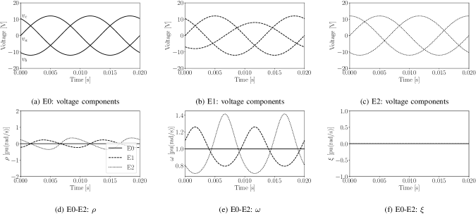
Figure 1: E0-E2: Three-phase AC voltage components, and geometric invariants $\rho$, $\omega$ and $\xi$.

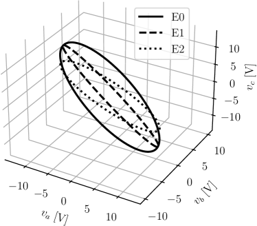
Figure 2: Three-phase voltage in the space $(v_{a},v_{b},v_{c})$, E0-E2.

Stationary Voltages

Assuming that the voltage is stationary with constant angular frequency $w_{o}$, the three components of the vector are:

$$v_{a} =V_{a}\sin(w_{o}t+\theta_{ao})\,,$$ (62)

$$v_{b} =V_{b}\sin(w_{o}t+\theta_{bo})\,,$$

$$v_{c} =V_{c}\sin(w_{o}t+\theta_{co})\,,$$

where $V_{i}$ is the voltage magnitude of phase $i$; and $\theta_{io}$ denotes the voltage angle of phase $i$ at $t=0$ s. Let $w_{o}=100\pi$ rad/s, $\theta_{ao}=0$ rad. Next, we consider relevant special cases of (58).

Positive and negative sequence voltages

From (59)-(61), one has for the stationary positive sequence with $V_{a}=V_{b}=V_{c}=\rm const.$ and $\theta_{bo}=-\theta_{co}=-{2\pi}/{3}$ rad:

$$\rho=\xi=0\,,\quad\boldsymbol{\omega}=\frac{w_{o}}{\sqrt{3}}(\boldsymbol{\rm e}_{\rm 1}+\boldsymbol{\rm e}_{\rm 2}+\boldsymbol{\rm e}_{\rm 3})\,.$$

Analogously, the stationary negative sequence, namely $V_{a}=V_{b}=V_{c}=\rm const.$ and $\theta_{bo}=-\theta_{co}={2\pi}/{3}$ rad, leads to:

$$\rho=\xi=0\,,\quad\boldsymbol{\omega}=-\frac{w_{o}}{\sqrt{3}}(\boldsymbol{\rm e}_{\rm 1}+\boldsymbol{\rm e}_{\rm 2}+\boldsymbol{\rm e}_{\rm 3})\,.$$

Hence, for the stationary positive and negative sequences, the time derivative operator (30) becomes:

$$D^{\boldsymbol{v}}_{t}=\frac{d}{dt}\mp\frac{w_{o}}{\sqrt{3}}[(\boldsymbol{\rm e}_{\rm 1}+\boldsymbol{\rm e}_{\rm 2}+\boldsymbol{\rm e}_{\rm 3})\times]\,,$$ (63)

and, as in the example of Section V.B, $\omega=|\boldsymbol{\omega}|=w_{o}$, namely the azimuthal and angular frequencies coincide.

Unbalanced voltage

Unbalanced voltages are characterized by $V_{a}\neq V_{b}\neq V_{c}$ and/or $\theta_{bo}\neq-\theta_{co}\neq-2\pi/3$ rad. Then, assuming that the voltage magnitudes and phase shifts are constants, from (59)-(61), one has:

$$\rho =\frac{w_{o}\sum_{i}V_{i}^{2}\sin(2\theta_{i})}{v^{2}}\,,\quad \xi=0\,,$$

$$\boldsymbol{\omega} =\frac{w_{o}\sum_{ijk}V_{j}V_{k}\sin(\theta_{j}-\theta_{k})\boldsymbol{\rm e}_{\rm i}}{v^{2}}\,.$$

In this case, thus, the components of the time derivative in (28) depend on the parameters of the voltage.

Zero-sequence voltage

This example allows us discussing the issue of the choice of the basis for the voltage vector. A zero-sequence voltage is composed of three equal AC voltages. In this case, thus, we cannot utilize the same coordinates we have used in the previous two examples, namely $(v_{a},v_{b},v_{c})$, as these are linearly dependent and do not form a basis. One has to proceed as discussed in Section V-B for a single-phase AC voltage, for which $\boldsymbol{\omega}=w_{o}\,\boldsymbol{\rm e}_{\rm 3}$. Thus, when considering three-phase voltages, one should thus first remove the zero-sequence from the voltage signals. This is common practice, anyway, for the zero-sequence to be generally treated separately or simply just removed from the positive and negative ones in power system measurements and protections.

Next, we illustrate (62) through the following examples.

$$\rm{E0:}\quad V_{a}=V_{b}=V_{c}=12~{}{\rm V}\,,$$

$$\theta_{bo}=-\theta_{co}=-{2\pi}/{3}~{}{\rm rad}\,.$$

$$\rm{E1:}\quad V_{a}=12~{}{\rm V}\,,\ \ V_{b}=8~{}{\rm V}\,,\ \ V_{c}=12~{}{\rm V}\,,$$

$$\theta_{bo}=-\theta_{co}=-{2\pi}/{3}~{}{\rm rad}\,.$$

$$\rm{E2:}\quad V_{a}=V_{b}=V_{c}=12~{}{\rm V}\,,$$

$$\theta_{bo}=-{2\pi}/{3}~{}{\rm rad}\,,\ \ \theta_{co}={1.5\pi}/{3}~{}{\rm rad}\,.$$

Figure 1 shows the phase voltages as well as the symmetric component of the geometric frequency ($\rho$), the Euclidean norm of the vector component ($\omega$), and the torsional frequency ($\xi$) for examples E0 to E2. Figure 2 illustrates the curve formed by the three-phase voltage in the space $(v_{a},v_{b},v_{c})$. Notice that $\xi=0$ holds for the three cases. This is consistent with the fact that each curve in Fig. 2 lies in a plane.

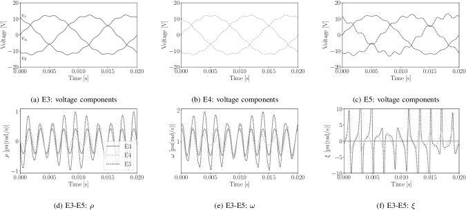
Figure 3: Three-phase voltage components, and geometric invariants $\rho$, $\omega$ and $\xi$, E3-E5.

V-D Three-Phase AC Voltages with Harmonics

In this section, we consider the case of three-phase voltages with harmonics. The conventional Fourier analysis define a basis that consists of as many dimensions as harmonics. While the proposed approach can be also utilized in an arbitrary $n$-dimensional space, we illustrate the consequences of the proposed approach in the same three-dimensional space we have utilized in the previous section.

Let the voltage vector in (57) also include a harmonic voltage component. Then, the three-phase voltage becomes:

$$v_{a} =V_{a}{\sin}(w_{o}t+\theta_{ao})+V_{a,h}{\sin}(hw_{o}t+\theta_{ao,h})\,,$$ (64)

$$v_{b} =V_{b}{\sin}(w_{o}t+\theta_{bo})+V_{b,h}{\sin}(hw_{o}t+\theta_{bo,h})\,,$$

$$v_{c} =V_{c}{\sin}(w_{o}t+\theta_{co})+V_{c,h}{\sin}(hw_{o}t+\theta_{co,h})\,,$$

where $V_{i,h}$ is the magnitude of the $h$-th harmonic of phase $i$; $\theta_{io,h}$ is the angle of the $h$-th harmonic of phase $i$ at $t=0$ s. Let $V_{a}=V_{b}=V_{c}=12$ V, $\theta_{bo}=-\theta_{co}=-{2\pi}/{3}$ rad. For the sake of example, we consider the following cases of (64): E3, balanced voltage; E4, phase imbalance in the harmonic; E5, magnitude imbalance in the harmonic. The following values are used.

$${\rm E3}:\quad V_{a,11}=V_{b,11}=V_{c,11}=0.5~{}{\rm V}\,,$$

$$\theta_{bo,11}=-\theta_{co,11}=-{2\pi}/{3}~{}{\rm rad}\,.$$

$${\rm E4}:\quad V_{a,11}=V_{b,11}=V_{c,11}=0.5~{}{\rm V}\,,$$

$$\theta_{bo,11}=-{2.7\pi}/{3}~{}{\rm rad}\,\ \ \theta_{co,11}={2.7\pi}/{3}~{}{\rm rad}\,.$$

$${\rm E5}:\quad V_{a,11}=0.5~{}{\rm V}\,,\ \ V_{b,11}=0.9~{}{\rm V}\,,\ \ V_{c,11}=1.3~{}{\rm V}\,,$$

$$\theta_{bo,11}=-\theta_{co,11}=-{2\pi}/{3}~{}{\rm rad}\,.$$

The phase voltages for cases E3-E5 as well as the trajectories of $\rho$, $\omega$ and $\xi$ are shown in Fig. 3, while the curve that the vector $\boldsymbol{v}$ forms in the $(v_{a},v_{b},v_{b})$ space is illustrated for each case in Fig. 4. For the balanced case, i.e. E3, a plane curve is obtained which implies a null torsion, whereas the curves in E4 and E5 are three-dimensional and thus the torsion in these cases is non-zero. It is relevant to note that the proposed approach, differently from Fourier analysis or any other approach based on the projections of the signal on a kernel function (e.g., the periodic small-signal stability analysis [32], wavelets and the Hilbert-Huang transform [33]), does not need to increase the size of the basis to take into account harmonics.

Figure 4: Three-phase voltage in the $(v_{a},v_{b},v_{c})$ space, E3-E5.

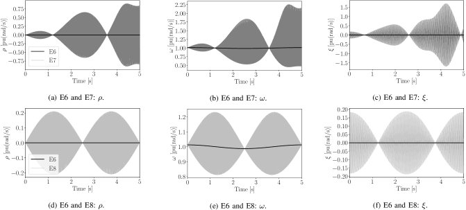
Figure 5: Geometric frequency components and torsional frequency, E6-E8.

V-E Three-Phase AC Voltages with Time-Variant Angular Frequency

In the previous section, we have discussed the difference between the Fourier approach and the proposed geometric approach. The latter utilizes a space that has always same dimensions regardless the number of harmonics present in the voltage. In this section, we further illustrate the benefit of this frugality of dimensions. We consider in fact a three-phase voltage with time-varying angular frequency. In this case, the Fourier transform would require a basis with infinitely many dimensions as the angular frequency varies continuously. The geometric approach, on the other hand, retains the three dimensions.

Let us consider that each component of the voltage vector in (57) has a time-varying frequency $w_{i}$, $i=\{a,b,c\}$. Then, the three AC voltage components are:

$$v_{a} =V_{a}\,{\sin}(w_{o}t+\theta_{a}(t)+\theta_{ao})\,,$$ (65)

$$v_{b} =V_{b}\,{\sin}(w_{o}t+\theta_{b}(t)+\theta_{bo})\,,$$

$$v_{c} =V_{c}\,{\sin}(w_{o}t+\theta_{c}(t)+\theta_{co})\,.$$

Let $V_{a}=V_{b}=V_{c}=12$ V, $w_{o}=100\pi$ rad/s, $\theta_{bo}=-\theta_{co}=-{2\pi}/{3}$ rad. As an example, we consider the following cases of (65): E6, balanced $\theta_{i}$; E7, frequency imbalance in $\theta_{i}$; and E8, magnitude imbalance in $\theta_{i}$. The following values are assumed.

$${\rm E6}:\quad \theta_{a}=\theta_{b}=\theta_{c}=\pi\sin(0.4\pi t)\,.$$

$${\rm E7}:\quad \theta_{a}=\theta_{b}=\pi\sin(0.4\pi t)\,,$$

$$\theta_{c}=\pi\sin(0.44\pi t)\,.$$

$${\rm E8}:\quad \theta_{a}=\theta_{b}=\pi\sin(0.4\pi t)\,,$$

$$\theta_{c}=1.1\pi\sin(0.4\pi t)\,.$$

Example E6 is representative of the transient following a contingency in a power system, where the oscillations of the phase angles of the voltages are due to the electro-mechanical swings of the synchronous machines. On the other hand, examples E7 and E8 do not represent a situation that can occur in a power system but are nevertheless relevant to show the effects of the torsional frequency.

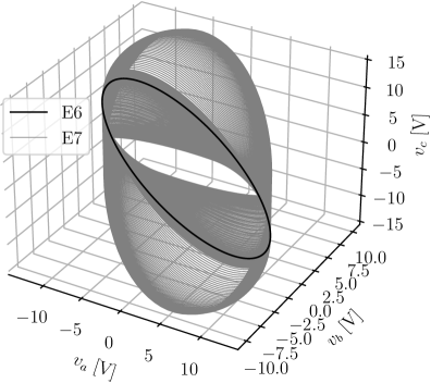
Figure 6: Three-phase voltage in $(v_{a},v_{b},v_{c})$ space, E6 and E7.

Figure 5 shows $\rho$, $\omega$ and $\xi$ for cases E6-E8. In the balanced case, i.e. E6, the three-phase voltages show the same frequency variation and null $\rho$ and $\xi$. The three-dimensional representation of $\boldsymbol{v}$ in the space $v_{a}$-$v_{b}$-$v_{c}$ is shown in Figs. 6 and 7. For E7 and E8, the period of the voltage is varying with time yet not in the same way in all three phases, thus leading to the curves shown in Figs. 6 and 7.

Figure 8 shows how the magnitude of the rate of change of the vector frequency ($|\boldsymbol{\omega}^{\prime}|$) compares to the magnitude of its symmetric component, i.e. $|\eta{\boldsymbol{\omega}}|$ (see equation (36)) for the three examples E6-E8. These two quantities are equal only at the time instants when the torsion is null or, equivalently, when $\xi=0$ (see Fig. 5f). It is also interesting to observe how unbalanced harmonics lead to large variations of $|\boldsymbol{\omega}^{\prime}|$.

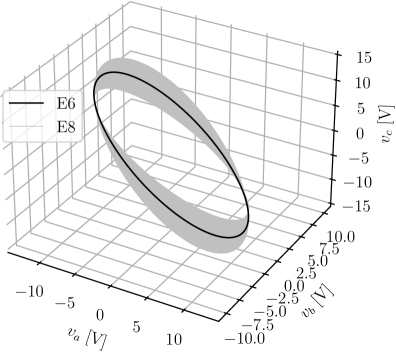
Figure 7: Three-phase voltage in $(v_{a},v_{b},v_{c})$ space, E6 and E8.

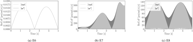
Figure 8: Magnitudes of $\boldsymbol{\omega}^{\prime}$ and its symmetrical component $\omega^{\prime}=|\eta\boldsymbol{\omega}|$, E6-E8.

V-F Park Transform

In this final example, we consider the time derivative of the voltage in the Park reference frame. Let us consider a voltage vector in the $\rm dqo$ coordinates:

$$\boldsymbol{v}=v_{\rm d}\,\boldsymbol{\rm e}_{\rm d}+v_{\rm q}\,\boldsymbol{\rm e}_{\rm q}+v_{\rm o}\,\boldsymbol{\rm e}_{\rm o}\,.$$ (66)

The time derivative of this vector in the “inertial” reference is given by:

$$\boldsymbol{v}^{\prime}=(v^{\prime}_{\rm d}-w_{\rm dq}v_{\rm q})\,\boldsymbol{\rm e}_{\rm d}+(v^{\prime}_{\rm q}+w_{\rm dq}v_{\rm d})\,\boldsymbol{\rm e}_{\rm q}+v^{\prime}_{\rm o}\,\boldsymbol{\rm e}_{\rm o}\,,$$ (67)

where $w_{\rm dq}$ is the angular speed of the Park reference frame and we have assumed a choice of the $\rm dqo$-axis such that $\boldsymbol{\rm e}^{\prime}_{\rm d}=w_{\rm dq}\boldsymbol{\rm e}_{\rm q}$, $\boldsymbol{\rm e}^{\prime}_{\rm q}=-w_{\rm dq}\boldsymbol{\rm e}_{\rm d}$, and $\boldsymbol{\rm e}^{\prime}_{\rm o}=\boldsymbol{0}$ [1].

The time derivative in the inertial reference in (67) is composed of two parts, namely the derivative in the rotating $\rm dqo$-axis frame plus the effect of rotation:

$$\boldsymbol{v}^{\prime}=\hat{\boldsymbol{v}}^{\prime}+\boldsymbol{r}\times\boldsymbol{v}\,,$$ (68)

where:

$$\hat{\boldsymbol{v}}^{\prime}=v^{\prime}_{\rm d}\,\boldsymbol{\rm e}_{\rm d}+v^{\prime}_{\rm q}\,\boldsymbol{\rm e}_{\rm q}+v^{\prime}_{\rm o}\,\boldsymbol{\rm e}_{\rm o}\,,$$ (69)

and

$$\boldsymbol{r}=w_{\rm dq}\,\boldsymbol{\rm e}_{\rm o}\,.$$ (70)

Next, we apply (28) and show that the proposed approach leads to the same results as (67) but with a different structure of the components of $\boldsymbol{v}^{\prime}$ with respect to (68). The quantities $\rho$ and $\boldsymbol{\omega}$ are:

$$\rho=\frac{v_{\rm d}v^{\prime}_{\rm d}+v_{\rm q}v^{\prime}_{\rm q}+v_{\rm o}v^{\prime}_{\rm o}}{v^{2}}\,,$$ (71)

and

$$\boldsymbol{\omega}= \frac{v_{\rm q}v^{\prime}_{\rm o}-v_{\rm o}v^{\prime}_{\rm q}-w_{\rm dq}v_{\rm o}v_{\rm d}}{v^{2}}\,\boldsymbol{\rm e}_{\rm d}+$$ (72)

$$\frac{v_{\rm o}v^{\prime}_{\rm d}-v_{\rm d}v^{\prime}_{\rm o}-w_{\rm dq}v_{\rm o}v_{\rm q}}{v^{2}}\,\boldsymbol{\rm e}_{\rm q}+$$

$$\frac{v_{\rm d}v^{\prime}_{\rm q}-v_{\rm q}v^{\prime}_{\rm d}+w_{\rm dq}(v_{\rm d}^{2}+v_{\rm q}^{2})}{v^{2}}\,\boldsymbol{\rm e}_{\rm o}\,,$$

where $v^{2}=v_{\rm d}^{2}+v_{\rm q}^{2}+v_{o}^{2}$. Although requiring some tedious algebraic manipulations, it is not difficult to show that, in fact, $\rho\boldsymbol{v}+\boldsymbol{\omega}\times\boldsymbol{v}$ is equal to the right-hand side of (67). On the other hand, it is straightforward to observe that:

$$\hat{\boldsymbol{v}}^{\prime}\neq\rho\boldsymbol{v}\,,\qquad\boldsymbol{r}\times\boldsymbol{v}\neq\boldsymbol{\omega}\times\boldsymbol{v}\,,$$ (73)

i.e., $\hat{\boldsymbol{v}}^{\prime}$ is not equal to the symmetric component of the time derivative and the term $\boldsymbol{r}\times\boldsymbol{v}$ is not equal to the antisymmetric component of the time derivative.

A relevant case is for $v_{o}=0$, namely balanced conditions, which leads to:

$$\rho=\frac{v_{\rm d}v_{\rm d}^{\prime}+v_{\rm q}v_{\rm q}^{\prime}}{v^{2}}\,,\quad\boldsymbol{\omega}=\frac{v_{\rm d}v^{\prime}_{\rm q}-v_{\rm q}v^{\prime}_{\rm d}+w_{\rm dq}v^{2}}{v^{2}}\,\boldsymbol{\rm e}_{\rm o}\,,$$ (74)

where $v^{2}=v_{\rm d}^{2}+v_{\rm q}^{2}$. We note that $\rho=v^{\prime}/v$, as expected, and:

$$\frac{v_{\rm d}v^{\prime}_{\rm q}-v^{\prime}_{\rm d}v_{\rm q}}{v^{2}}=\frac{d}{dt}\arctan\left(\frac{v_{\rm q}}{v_{\rm d}}\right)=\Delta\omega\,,$$ (75)

which is the deviation of the angular frequency of $\boldsymbol{v}$ with respect to $w_{\rm dq}$. Hence the inertial- and rotating-frame time derivatives of the voltage can be written as:

$$\boldsymbol{v}^{\prime}=\rho\boldsymbol{v}+(w_{\rm dq}+\Delta\omega)\,\boldsymbol{\rm e}_{\rm o}\times\boldsymbol{v}\,,$$ (76)

and:

$$\hat{\boldsymbol{v}}^{\prime}=\rho\boldsymbol{v}+\Delta\omega\,\boldsymbol{\rm e}_{\rm o}\times\boldsymbol{v}\,.$$ (77)

The following remarks are relevant.

Remark 5

The only case for which $\rho\boldsymbol{v}=\hat{\boldsymbol{v}}^{\prime}$ and $\boldsymbol{r}\times\boldsymbol{v}=\boldsymbol{\omega}\times\boldsymbol{v}$ is if the angular speed of the Park transform is the actual frequency of $\boldsymbol{v}$. In this case, in fact, $\Delta\omega=0$. This result is consistent with the commonly-used Park-Concordia model of the synchronous machine [34].

Remark 6

The Clarke transform can be viewed as a special case of the Park transform, with $w_{\rm dq}=0$. In this case (68) leads to $\boldsymbol{v}^{\prime}=\hat{\boldsymbol{v}}^{\prime}$. This result is consistent with (76).

Remark 7

In stationary conditions, i.e., for $v^{\prime}_{\rm d}=v^{\prime}_{\rm q}=0$, (76) leads to the same expression as (50), thus confirming that balanced stationary three-phase voltages are equivalent to a single-phase phasor.

V-G IEEE 39-Bus System

This example shows the application of the proposed formulas to estimate $\omega$, $\rho$, and $\xi$ at a bus of a power system following a contingency. To this aim, we use the model of the IEEE 39-bus system for Electro-Magnetic Transient (EMT) simulations provided by DIgSILENT PowerFactory. The system model is based on the original IEEE 39-bus benchmark network, which has been modified to capture the behavior during EMTs of the power network, namely, the frequency dependency of transmission lines and the non-linear saturation of transformers.

The system is numerically integrated assuming a phase-to-phase fault between phases $a$ and $b$ at terminal bus 3 of the system at $t=0.2$ s. The fault is cleared at $t=0.3$ s. The integration time step considered is $10^{-5}$ s. The phase voltages at bus 26 following the contingency are shown in Fig. 9, while the curve formed by the three-phase voltage in the space $(v_{a},v_{b},v_{c})$ is illustrated in Fig. 10. Figure 11 shows $\omega$, $\rho$, and $\xi$ following the contingency, where first-order filtering has been applied to smooth the numerical noise in the calculation of the voltage vector time derivatives. Before the occurrence of the fault, the three phases are balanced and thus, the corresponding part of the curve in Fig. 10 is circular and lies in a plane. The same holds after the fault clearance. Results also indicate that before the occurrence and after the clearance of the fault, both $\rho$ and $\xi$ are null, which is consistent to the discussion of Section V-E (e.g., example E6). On the other hand, the voltage phases are unbalanced during the fault, which gives rise to the non-circular and non-planar sections observed in Fig. 10. For this part, both $\rho$ and $\xi$ are non-zero as shown in Fig. 11. This is again consistent with Section V-E and in particular with the discussion of example E8. Furthermore, $\omega$ accurately captures the primary frequency response at bus 26 following the contingency (see Fig. 11b).

Finally, for the sake of comparison, we mention that the differences of the IEEE 39-bus system with respect to the results of E8 are that (i) the frequency oscillation is damped and reaches a new steady state condition, whereas this does not hold for E8, and (ii) the imbalance occurs only for few voltage cycles, whereas in E8 voltages are unbalanced during the whole simulation, which is the reason why the curve in Fig. 10 does not appear like a compact three-dimensional object as is the case in Fig. 7.

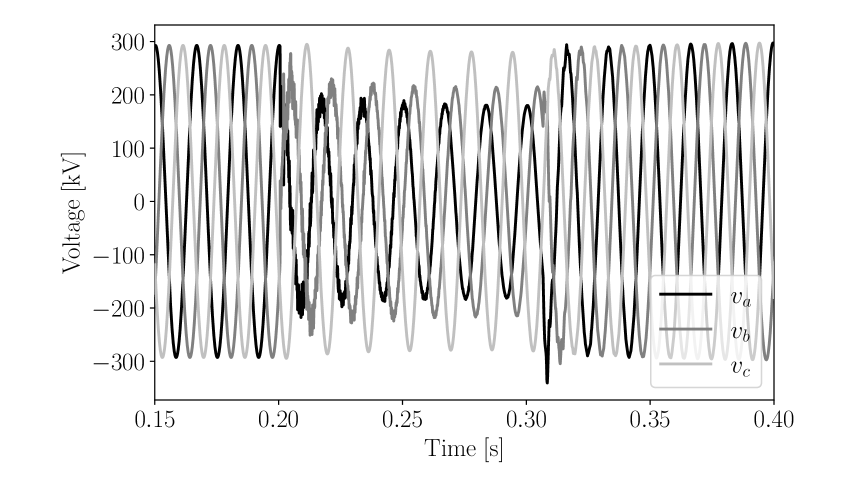
Figure 9: Three-phase voltage at bus 26, IEEE 39-bus system.

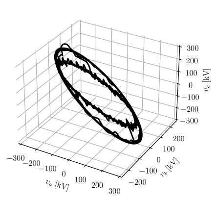
Figure 10: Three-phase voltage at bus 26 in the space $(v_{a},v_{b},v_{c})$, IEEE 39-bus system.

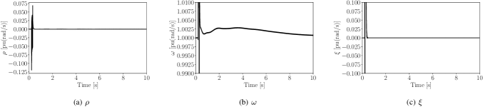
Figure 11: Geometric invariants $\rho$, $\omega$ and $\xi$ at bus 26, IEEE 39-bus system.

VI Conclusions

The paper elaborates on the geometrical interpretation of electric quantities and deduces several expressions that link the time derivatives of the voltage, current and frequency in electrical circuits with the Frenet frame. Among these expressions, we mention in particular (28) and (37). Equation (28) indicates that the time derivative of the voltage (and the current) is composed of two parts, one symmetric, that depends only on the magnitude, and one antisymmetric that depends on the “rotation” of the quantity itself. Equation (37) shows that the time derivative of the vector frequency is more complex than the common notion of RoCoF and includes a “rotational” and a “torsional” component. The latter is defined in this paper for the first time. It is interesting to note that the antisymmetric component of the RoCoF may affect the implementation and/or performance of existing controllers. Since the proposed approach allows separating the symmetric and antisymmetric terms, it appears as a useful tool for the study of power system transients and the design of controllers. More in general, we believe that the proposed approach may find relevant applications in estimation, control and stability analysis of power systems.

The proposed theory is certainly more complex than the current conventional approach based on phasors. However, it shows added values from the theoretical point of view, as follows.

• It is a generalization of the conventional approach. The conventional approach, in fact, appears to be a special case of the proposed theory.

• It is an example of interdisciplinary approach. Differential geometry and the Frenet frame, in fact, were originally developed for mechanical systems. Their applications, under certain hypotheses, to electrical circuits appears as an interesting advance which paves the way to several further developments.

An interesting byproduct of the latter point is that the proposed theory allows “visualizing” electrical quantities. This is important, as, in the experience of the first author, students always struggle with the lack of visual aid when studying circuit theory. Such a support is a given in mechanical engineering. Thus, the ability to re-utilize well-known concepts such as curvature and torsion also adds a didactic value to the proposed approach.

We anticipate several future work directions. Among these, we mention the development of a geometric framework for circuit analysis; the applications of the formulas to estimate unbalanced conditions in three-phase circuits as well as to circuits with more than three phases using Cartan’s extensions of the Frenet framework (see, e.g., [35]); and the development of active controllers to reduce the effect of harmonics and imbalances.

In this appendix, we prove the identity $n=\omega v$. From (20) on has:

$$\omega=\frac{|\boldsymbol{\omega}|}{v^{2}}=\frac{|\boldsymbol{v}\times\boldsymbol{v}^{\prime}|}{v^{2}}\,.$$ (78)

Let us focus on the term $|\boldsymbol{v}\times\boldsymbol{v}^{\prime}|$. This can be written as:

$$|\boldsymbol{v}\times\boldsymbol{v}^{\prime}|=\sqrt{(\boldsymbol{v}\times\boldsymbol{v}^{\prime})\cdot(\boldsymbol{v}\times\boldsymbol{v}^{\prime})}\,.$$ (79)

From the following identity of the triple scalar product:

$$\boldsymbol{a}\cdot\boldsymbol{b}\times\boldsymbol{c}=\boldsymbol{b}\cdot\boldsymbol{c}\times\boldsymbol{a}\,,$$ (80)

equation (79) can be rewritten as:

$$|\boldsymbol{v}\times\boldsymbol{v}^{\prime}|=\sqrt{\boldsymbol{v}\cdot\boldsymbol{v}^{\prime}\times(\boldsymbol{v}\times\boldsymbol{v}^{\prime})}\,.$$ (81)

Then, from the following identity of the triple vector product:

$$(\boldsymbol{a}\times\boldsymbol{b})\times\boldsymbol{c}=(\boldsymbol{a}\cdot\boldsymbol{c})\,\boldsymbol{b}-(\boldsymbol{b}\cdot\boldsymbol{c})\,\boldsymbol{a}\,,$$ (82)

equation (81) can be rewritten as:

$$|\boldsymbol{v}\times\boldsymbol{v}^{\prime}|=\sqrt{\boldsymbol{v}\cdot[(\boldsymbol{v}^{\prime}\cdot\boldsymbol{v}^{\prime})\boldsymbol{v}-(\boldsymbol{v}^{\prime}\cdot\boldsymbol{v})\boldsymbol{v}^{\prime}]}\,.$$ (83)

From (20) and (18), the previous expression is equivalent to:

$$|\boldsymbol{v}\times\boldsymbol{v}^{\prime}| =\sqrt{(\boldsymbol{v}^{\prime}\cdot\boldsymbol{v}^{\prime})(\boldsymbol{v}\cdot\boldsymbol{v})-(\boldsymbol{v}\cdot\boldsymbol{v}^{\prime})^{2}}$$ (84)

$$=\sqrt{|\boldsymbol{v}^{\prime}|^{2}v^{2}-\rho^{2}v^{4}}\,,$$

and, hence, (78) becomes:

$$\omega=\frac{\sqrt{|\boldsymbol{v}^{\prime}|^{2}-\rho^{2}v^{2}}}{v}\,,$$ (85)

which, recalling the definition of $n$ given in (23), demonstrates that $n=\omega v$ and, hence, $\boldsymbol{n}=\boldsymbol{\omega}\times\boldsymbol{v}$. From this relationship and the properties of the vectors of the Frenet frame, the following relationships follow:

$$\boldsymbol{v}=\frac{\boldsymbol{n}\times\boldsymbol{\omega}}{\omega^{2}}\,,\qquad\boldsymbol{\omega}=\frac{\boldsymbol{v}\times\boldsymbol{n}}{v^{2}}\,.$$ (86)

Federico Milano (F’16) received from the Univ. of Genoa, Italy, the ME and Ph.D. in Electrical Engineering in 1999 and 2003, respectively. From 2001 to 2002 he was with the University of Waterloo, Canada, as a Visiting Scholar. From 2003 to 2013, he was with the Universtiy of Castilla-La Mancha, Spain. In 2013, he joined the University College Dublin, Ireland, where he is currently Professor of Power Systems Protection and Control. He is an IEEE PES Distinguished Lecturer, an editor of the IEEE Transactions on Power Systems and an IET Fellow. He is the chair of the IEEE Power System Stability Controls Subcommittee. His research interests include power system modelling, control and stability analysis.

Georgios Tzounas (M’21) received from National Technical University of Athens, Greece, the Diploma (ME) in Electrical and Computer Engineering in 2017, and the Ph.D. in Electrical Engineering from University College Dublin, Ireland, in 2021. He is currently a post doctoral researcher with University College Dublin, working on the Horizon 2020 project edgeFLEX. His research interests include modelling, stability analysis, and automatic control of power systems.

Ioannis Dassios received his Ph.D. in Applied Mathematics from the Dpt of Mathematics, Univ. of Athens, Greece, in 2013. He worked as a Postdoctoral Research and Teaching Fellow in Optimization at the School of Mathematics, Univ. of Edinburgh, UK. He also worked as a Research Associate at the Modelling and Simulation Centre, University of Manchester, UK, and as a Research Fellow at MACSI, Univ. of Limerick, Ireland. He is currently a UCD Research Fellow at UCD, Ireland.

Taulant Kërçi (S’18) received from the Polytechnic University of Tirana, Albania, the BSc. and MSc. degree in Electrical Engineering in 2011 and 2013, respectively. From June 2013 to October 2013, he was with the Albanian DSO at the metering and new connection department. From November 2013 to January 2018, he was with the TSO at the SCADA/EMS office. Since February 2018, he is a Ph.D. candidate with UCD, Ireland. In September 2021, he joined the Irish TSO, EirGrid. His research interests include power system dynamics and co-simulation of power systems and electricity markets.

References

- [1] F. Milano and Á. Ortega, Frequency Variations in Power Systems: Modeling, State Estimation, and Control. Hoboken, NJ: Wiley, 2020.
- [2] J. J. Stoker, Differential Geometry. New York: Wiley, 1969.
- [3] N. Yokoya and M. Levine, “Range image segmentation based on differential geometry: a hybrid approach,” IEEE Trans. on Pattern Analysis and Machine Intelligence, vol. 11, no. 6, pp. 643–649, 1989.
- [4] J. Selig, Geometric Fundamentals of Robotics, 2nd ed. New York: Springer, 2005.
- [5] L. Lapierre, D. Soetanto, and A. Pascoal, “Nonlinear path following with applications to the control of autonomous underwater vehicles,” in 42nd IEEE Int. Conf. on Decision and Control, vol. 2, 2003, pp. 1256–1261.
- [6] M. Werling, J. Ziegler, S. Kammel, and S. Thrun, “Optimal trajectory generation for dynamic street scenarios in a Frenét frame,” in IEEE Int. Conf. on Robotics and Automation, 2010, pp. 987–993.
- [7] A. Hanson and H. Ma, “Quaternion frame approach to streamline visualization,” IEEE Trans. on Visualization and Computer Graphics, vol. 1, no. 2, pp. 164–174, 1995.
- [8] J. Selig, Quaternions for Computer Graphics. New York: Springer, 2011.
- [9] S. P. Talebi, S. Werner, and D. P. Mandic, “Quaternion-valued distributed filtering and control,” IEEE Trans. on Automatic Control, vol. 65, no. 10, pp. 4246–4257, 2020.
- [10] J. L. Willems, “Mathematical foundations of the instantaneous power concepts: A geometrical approach,” European Trans. on Electrical Power, vol. 6, no. 5, pp. 299–304, 1996.
- [11] X. Dai, G. Liu, and R. Gretsch, “Generalized theory of instantaneous reactive quantity for multiphase power system,” IEEE Trans. on Power Delivery, vol. 19, no. 3, pp. 965–972, 2004.
- [12] A. Menti, T. Zacharias, and J. Milias-Argitis, “Geometric algebra: A powerful tool for representing power under nonsinusoidal conditions,” IEEE Trans. on Circuits and Systems - I: Regular Papers, vol. 54, no. 3, pp. 601–609, 2007.
- [13] M. Castilla, J. C. Bravo, M. Ordonez, and J. C. Montano, “Clifford theory: A geometrical interpretation of multivectorial apparent power,” IEEE Trans. on Circuits and Systems - I: Regular Papers, vol. 55, no. 10, pp. 3358–3367, 2008.
- [14] H. Lev-Ari and A. M. Stankovic, “Instantaneous power quantities in polyphase systems – A geometric algebra approach,” in IEEE Energy Conversion Congress and Exposition, 2009, pp. 592–596.
- [15] H. Akagi, E. H. Watanabe, and M. Aredes, Instantaneous Power Theory and Applications to Power Conditioning, 2nd ed. New York: Wiley IEEE Press, 2017.
- [16] F. G. Montoya, R. Baños, A. Alcayde, F. M. Arrabal-Campos, and J. Roldán-Pérez, “Vector geometric algebra in power systems: An updated formulation of apparent power under non-sinusoidal conditions,” Mathematics, vol. 9, no. 11, 2021.
- [17] M. Castro-Núñez and R. Castro-Puche, “Advantages of geometric algebra over complex numbers in the analysis of networks with nonsinusoidal sources and linear loads,” IEEE Trans. on Circuits and Systems - I: Regular Papers, vol. 59, no. 9, pp. 2056–2064, 2012.
- [18] N. Barry, “The application of quaternions in electrical circuits,” in 2016 27th Irish Signals and Systems Conference (ISSC), 2016, pp. 1–9.
- [19] V. d. P. Brasil, A. de Leles Ferreira Filho, and J. Y. Ishihara, “Electrical three phase circuit analysis using quaternions,” in 18th Int. Conf. on Harmonics and Quality of Power (ICHQP), 2018, pp. 1–6.
- [20] S. P. Talebi and D. P. Mandic, “A quaternion frequency estimator for three-phase power systems,” in IEEE Int. Conf. on Acoustics, Speech and Signal Processing (ICASSP), 2015, pp. 3956–3960.
- [21] F. Milano, “A geometrical interpretation of frequency,” 2021, submitted to IEEE PESL, available at https://arxiv.org/abs/2105.07762.
- [22] F. Milano, F. Dörfler, G. Hug, D. J. Hill, and G. Verbič, “Foundations and challenges of low-inertia systems (invited paper),” in 2018 Power Systems Computation Conference (PSCC), 2018, pp. 1–25.
- [23] P. Castello, R. Ferrero, P. A. Pegoraro, and S. Toscani, “Effect of unbalance on positive-sequence synchrophasor, frequency, and rocof estimations,” IEEE Trans. on Instrumentation and Measurement, vol. 67, no. 5, pp. 1036–1046, 2018.
- [24] G. Frigo, A. Derviškadić, Y. Zuo, and M. Paolone, “Pmu-based rocof measurements: Uncertainty limits and metrological significance in power system applications,” IEEE Trans. on Instrumentation and Measurement, vol. 68, no. 10, pp. 3810–3822, 2019.
- [25] A. K. Singh and B. C. Pal, “Rate of change of frequency estimation for power systems using interpolated dft and kalman filter,” IEEE Trans. on Power Systems, vol. 34, no. 4, pp. 2509–2517, 2019.
- [26] G. Rietveld, P. S. Wright, and A. J. Roscoe, “Reliable rate-of-change-of-frequency measurements: Use cases and test conditions,” IEEE Trans. on Instrumentation and Measurement, vol. 69, no. 9, pp. 6657–6666, 2020.
- [27] S. Azizi, M. Sun, G. Liu, and V. Terzija, “Local frequency-based estimation of the rate of change of frequency of the center of inertia,” IEEE Trans. on Power Systems, vol. 35, no. 6, pp. 4948–4951, 2020.
- [28] L. Cohen, Time Frequency Analysis: Theory and Applications. Upper Saddle River, NJ: Prentice-Hall Signal Processing, 1995.
- [29] S. L. Hahn, Hilbert Transforms in Signal Processing. Boston: Artech House, 1996.
- [30] K. Strunz, R. Shintaku, and F. Gao, “Frequency-adaptive network modeling for integrative simulation of natural and envelope waveforms in power systems and circuits,” IEEE Trans. on Circuits and Systems - I: Regular Papers, vol. 53, no. 12, pp. 2788–2803, 2006.
- [31] “IEEE/IEC International Standard - Measuring relays and protection equipment - Part 118-1: Synchrophasor for power systems - Measurements,” pp. 1–78, 2018.
- [32] F. Bizzarri, A. Brambilla, and F. Milano, “Analytic and numerical study of TCSC devices: Unveiling the crucial role of phase-locked loops,” IEEE Trans. on Circuits and Systems - I: Regular Papers, vol. 65, no. 6, pp. 1840–1849, 2018.
- [33] N. E. Huang and S. S. P. Shen, Hilbert-Huang Transform and its Applications. Hackensack, NJ: World Scientific, 2014.
- [34] P. W. Sauer and M. A. Pai, Power System Dynamics and Stability. Upper Saddle River, NJ: Prentice Hall, 1998.
- [35] P. Griffiths, “On Cartan’s method of Lie groups and moving frames as applied to uniqueness and existence questions in differential geometry,” Duke Mathematical Journal, vol. 41, no. 4, pp. 775 – 814, 1974.