Symmetry-dependent exciton-exciton interaction and intervalley biexciton in monolayer transition metal dichalcogenides

Abstract

The multivalley band structure of monolayer transition metal dichalcogenides (TMDs) gives rise to intravalley and intervalley excitons. Much knowledge of these excitons has been gained, but fundamental questions remain, such as how to describe them all in a unified picture with their correlations, how are those from different valleys coupled to form the intervalley biexciton? To address the issues, we derive an exciton Hamiltonian from interpair correlations between the constituent carriers-fermions of two excitons. Identifying excitons by irreducible representations of their point symmetry group, we find their pairwise interaction depending on interacting excitons’ symmetry. It is generally repulsive, except for the case excitons from different valleys, which attract each other to form the intervalley biexciton. We establish a semianalytical relationship between the biexciton binding energy with exciton mass and dielectric characteristics of the material and surroundings. Overall, by providing insight into the nature of diverse excitons and their correlations, our theoretical model captures the exciton interaction properties permitting an inclusive description of the structure and energy features of the intervalley biexciton in monolayer TMDs.

I INTRODUCTION

Monolayer (ML) group-VI transition metal dichalcogenides (TMDs), such as MoS₂, MoSe₂, WS₂ and WSe₂, are two-dimensional (2D) semiconductors with direct band gaps at the edges $K$ and $K^{\prime}$ of the hexagonal Brillouin zone (BZ).^1,2 The reduced dielectric screening of the Coulomb interaction³ results in the formation of tightly bound excitons at the $K$ and $K^{\prime}$ valleys, dominating the optical response of the materials.^4,5 Besides the optically accessible bright excitons, the electronic structure of ML TMDs gives rice to inaccessible dark excitons, affecting different optical processes near the exciton resonance.^6-8 Despite numerous works on exciton physics, a unified picture of diverse excitons with their quantum correlations is still lacking. Thus the understanding of such an exciton fundamental feature as the exciton-exciton interaction remains limited. Scarce theoretical studies consider only the intravalley interaction between identical bright excitons, showing that it is repulsive in the exciton ground state.^9,10 Meanwhile, experiments report signatures of the intervalley biexciton in various ML TMDs^11-18 indicating an intervalley attractive exciton-exciton interaction. The attraction between excitons from opposite valleys certainly has a connection with the intervalley coupling between their constituent charge carriers via the Coulomb interaction. Several authors groups have attempted to model the intervalley biexciton.^19-23 However, without the intervalley carrier-carrier interaction taken into consideration, they have not succeeded. In particular, their calculations give for the biexciton binding energy in different freestanding MLTMDs comparable values around 20 meV, whereas experimental reports are markedly diverse. Experiments show that the exciton-exciton interaction in ML TMDs is enhanced, offering perspectives for engineering exciton-mediated optical nonlinearities.²⁴ It qualitatively changes the physical picture of the coherent light-matter interaction in the optical Stark effect.^25-27 Especially, involvement of the intervalley biexciton makes this effect valley-dependent, giving a possibility for coherent manipulation of the exciton valley degree of freedom in quantum information.^28,29 Thus a comprehensive study of the exciton-exciton interaction and the intervalley biexciton is of necessity not only for fundamentals of many-body physics but also for promising quantum technologies applications.

To address the elusive issue, we derive an exciton Hamiltonian from correlations between the constituent charge carriers-fermions of two excitons, mediated by the electrostatic carrier-carrier interaction and the Pauli exclusion principle. Identifying each exciton by an irreducible representation of their point symmetry group, we find the exciton-exciton interaction depending on the interacting excitons’ symmetry. It is generally repulsive, except for the case excitons from different valleys, which attract each other. We elucidate the microscopic mechanism underlying the intervalley exciton-exciton attraction. We ascertain a substantial dependence of the intervalley interaction on the exciton radius, determining the overlap degree of the wave functions of distant excitons in the momentum space. Adopting the Kedysh potential for the carrier-carrier interaction,³ we have the exciton radius as the variational parameter.^30,31 We find it from a function established between the exciton binding energy with its mass and the material and environment dielectric characteristics. With values of the latter as input variables taken from experimental measures,^32,33 we find the intervalley interaction potential sufficiently weak to be considered a perturbation. As a result, the estimated biexciton binding energy has the form of an exponential function of the exciton mass and intervalley interaction energy.³⁴ Its sensitivity to every input variable can help understanding discrepancies between different experimental measurements.^11-18 In freestanding tungsten-based MLs with light excitons, the estimated binding energy is under 20 meV, while in ML MoSe₂ and MoS₂ with heavier excitons, it is about 65 meV and 53 meV, respectively. The last number is near the appropriate experimental measurement of Sie et al.¹² Studying the reduction of the biexciton binding energy with increasing environment screening, we find, e.g. that the biexciton binding energy in hBN encapsulated ML MoSe₂ falls to the range of 24 meV, going along with recent experimental findings.²⁷ The obtained dependence of the biexciton binding energy in ML TMDs on the average dielectric constant of their immediate surroundings might serve as guidelines for future experiments to study the biexciton feature in various dielectric environments. On the other hand, our symmetry-dependent exciton Hamiltonian would form a baseline for theoretical research on valley selective nonlinear effects in a coherently driven ML TMD.

RESULTS

Valley single-particle states and their interaction

We consider an ML TMD having direct band gaps with the conduction and valence band extrema at the $K$ and $K^{\prime}$ valleys. The point symmetry group of the material is $D_{3h}$, but at the valleys the wave vector group is $C_{3h}$. To exploit the group theoretical algebra elaborated for the point group, we classify the valley Bloch states by one-dimensional spinor (double-valued) representations of the $C_{3h}$ double group in Koster et al. notations.³⁵ Each spinor representation corresponds to a definite half-integral angular momentum value including the momentum $j$ and its projection $j_{z}$ on the $z$-axis. Thus the valley states can be alternatively identified by those of their angular momentum $|\,j,j_{z}\,\rangle$, which we will refer to shortly as spin and spin projection. Thanks to large valence band splittings,^36,37 we can exclude the lower spin-orbit split valence band from consideration by considering the selective excitation of the ground state A exciton. Under this condition, we sketch the band structure of ML TMDs at the $K$ and $K^{\prime}$ valleys in Fig. 1, where we take the tungsten-based (WX₂) subgroup with the order of conduction bands reverse to that in molybdenum-based (MoX₂) subgroup, X = S, Se.³⁸

A resonant light field applied to a direct-gap semiconductor raises electrons from the filled valence band into the empty conduction band. The promotion of an electron creates a pair of electronic states, including the conduction band electron and the empty state that it leaves in the valence band, as schematically shown in Fig. 1. The electric dipole interaction of a polarized light field propagating along axis $z$ with the system of created pair states is defined by the product $\mathbf{E}_{\lambda}\mathbf{d}$ with $\mathbf{d}$ the system electric dipole momentum and $\mathbf{E_{\lambda}\,}$the electric field of photons with spin projection $\lambda$ on the $z$-axis. The field $\mathbf{E_{\lambda}\propto\varepsilon}_{\lambda}$, where $\mathbf{\varepsilon}_{\lambda}$ is the polarization vector orthogonal to the direction of the light propagation. For the circularly polarized $\sigma_{+}$ and $\sigma_{-}$ light with $\lambda=1$ and $\lambda=-1$ respectively, the polarization vector $\mathbf{\varepsilon}_{\lambda}\propto(1+\lambda i)$.³⁹ Thus at normal incidence, the coupling of the optical field to the electronic system is determined by the matrix element of the dipole momentum $d_{\pm}=(d_{x}\pm id_{y})$ between the valence and conduction bands. Composing of components of a polar vector, $d_{+}$ and $d_{-}$ are transformed according to the representation $\Gamma_{2}$ and $\Gamma_{3}$ of the $C_{3h}$ group, respectively.³⁵ According to the group theory selection rules⁴⁰ and multiplication table of irreducible representations of the $C_{3h}$ double group, one has interband matrix elements $\left\langle\Gamma_{11}|d_{+}|\Gamma_{7}\right\rangle\neq 0$ and $\left\langle\Gamma_{12}|d_{-}|\Gamma_{8}\right\rangle\neq 0$, and $\left\langle\Gamma_{9}|d_{+}|\Gamma_{7}\right\rangle=\left\langle\Gamma_{10}|d_{-}|\Gamma_{8}\right\rangle=0$. In this way, direct transitions to the $\Gamma_{11}$ ($\Gamma_{9}$) conduction band at the $K\$valley and to $\Gamma_{12}$ ($\Gamma_{10}$) one at the $K^{\prime}\$valley from the respective valence band are dipole allowed (forbidden). The light of $\sigma_{+}$ circular polarization can create pair states exclusively at $K$ valley, while that of $\sigma_{-}$ polarization can do this only at $K^{\prime}\$valley. This is the valley-dependent optical selection rule.^36,41,42 To focus on the intervalley interaction between excitons, hereafter we will leave aside the split-off conduction bands that are connected with the intravalley dipole forbidden excitons (the lower bands in Fig. 1). Thus, we limit ourselves in this paper to a simplified model with two-band schemes at the $K$ and $K^{\prime}$ valleys. Because excitons are Coulomb-bound electron-hole pairs, we begin by considering the pairwise interaction among carriers. In the second quantization representation, the system of these single-particle states is described by Heisenberg creation and annihilation field operators $\Phi^{\dagger}(\mathbf{r})$ and $\Phi(\mathbf{r})$. The operator of any macroscopic physical quantity of the many-electron system, in particular the number of pair states and Hamiltonian, is presented in terms of $\Phi^{\dagger}(\mathbf{r})$ and $\Phi(\mathbf{r})$,⁴³

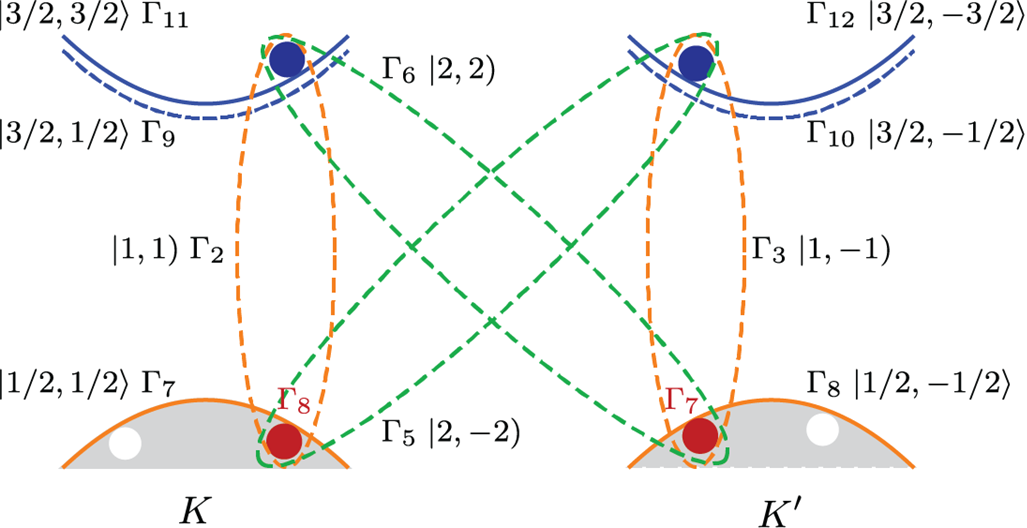
Figure 1: Sketch of the band structure of ML tungsten dichalcogenides at the $K$ and $K^{\prime}$ valleys and related excitons. Valley states and excitons are denoted by irreducible representations of the $C_{3h}$ double group with the corresponding spin states shown beside. Blue, white, and dark red balls depict conduction electrons, missing valence band electrons, and holes, respectively. Bright and dark excitons are represented by orange and green dashed ovals, respectively, incorporating corresponding electrons and holes.

$$N=\int d^{2}r\,\Phi^{\dagger}(\mathbf{r})\,\Phi(\mathbf{r})$$ (1)

$$H=\int d^{2}r\,\Phi^{\dagger}(\mathbf{r})\,\mathcal{H}_{c}\,\Phi(\mathbf{r})+\frac{1}{2}\int\int d^{2}r_{1}\,d^{2}r_{2}\,\Phi^{\dagger}(\mathbf{r}_{1})\Phi^{\dagger}(\mathbf{r}_{2})\,V_{K}(|\mathbf{r}_{1}-\mathbf{r}_{2}|)\,\Phi(\mathbf{r}_{2})\Phi(\mathbf{r}_{1})$$ (2)

where $\mathcal{H}_{c}$ is the Hamiltonian of a single crystal electron in the periodic lattice potential and $V(r)$ – nonlocally screened Coulomb potential describing the symmetric pairwise interaction between in-plain carriers. We adopt the Keldysh potential,³ which can be presented in the form

$$V_{K}(r)\simeq\frac{e^{2}}{\varepsilon_{0}r_{0}}\frac{\pi}{2}\left[H_{0}\left(\frac{\kappa r}{r_{0}}\right)-Y_{0}\left(\frac{\kappa r}{r_{0}}\right)\right]$$ (3)

where $e$ is the electron charge, $\varepsilon_{0}$ – the vacuum permittivity, $r_{0}$ – the effective screening length characterizing dielectric properties of an ML TMD, $\kappa=\left(\varepsilon_{t}+\varepsilon_{b}\right)/2$ with $\varepsilon_{t}$ and $\varepsilon_{b}$ the dielectric constants of the encapsulating materials above and below the ML, respectively, and $H_{0}$ and $Y_{0}$ – Struve and Bessel functions of the second kind. The screening length of an ML having width $d$ and dielectric constant $\varepsilon$ is defined as $r_{0}=d\varepsilon/\left(\varepsilon_{t}+\varepsilon_{b}\right)$ with $\varepsilon_{t}=\varepsilon_{b}=1$ (vacuum). In the strictly 2D limit $r_{0}=2\pi\chi_{2D}$, where $\chi_{2D}$ is the 2D polarizability of the planar material.⁴⁴ An inspection of Eq. (3) shows that the carrier-carrier interaction in ML TMDs weakens with increasing screening, either the ML screening ($r_{0}$) or that from the environment ($\kappa$). Thus the interaction can be ’tuned’ by selecting different immediate surroundings for the ML.

We expand field operators into the complete set of orthonormal Bloch functions – the eigenstates of $\mathcal{H}_{c}$,⁴⁵ $\phi_{\Gamma,\mathbf{k}}(\mathbf{r})=u_{\Gamma,\mathbf{k}}(\mathbf{r})\exp[i\mathbf{kr}]/\sqrt{S}$ with $S$ the sample area and $\Gamma$ the band states symmetry. With the assumption that under resonant excitation crystal electrons are accummulated primarily near $K$ and $K^{\prime}$ valleys, we can limit the expansion to the wave vectors around the valleys,

$$\Phi(\mathbf{r})\simeq\sum\limits_{\begin{subarray}{c}\Gamma=\Gamma_{11},\,\Gamma_{7}\\ \mathbf{p}\end{subarray}}{\large{e}_{\Gamma,\,\mathbf{p}}\,}\phi_{\Gamma,\,\mathbf{p}}(\mathbf{r})+\sum\limits_{\begin{subarray}{c}\Gamma=\Gamma_{12},\,\Gamma_{8}\\ \mathbf{p}^{\prime}\end{subarray}}{\large{e}_{\Gamma,\,\mathbf{p}^{\prime}}\,}\phi_{\Gamma,\,\mathbf{p}^{\prime}}(\mathbf{r})$$ (4)

where the sums are running over $\mathbf{p=k-K}$ and $\mathbf{p}^{\prime}\mathbf{=k-K}^{\prime}$, $p,p^{\prime}\ll\left|\mathbf{K}\right|,\left|\mathbf{K}^{\prime}\right|$, with $\mathbf{K}$ and $\mathbf{K}^{\prime}$ the positions of the BZ corner points in the k-space,

$$\mathbf{K=}\frac{2\pi}{3a}\left(1,\frac{1}{\sqrt{3}}\right),\qquad\mathbf{K}^{\prime}\mathbf{=}\frac{2\pi}{3a}\left(1,-\frac{1}{\sqrt{3}}\right)$$ (5)

($a$ is the lattice constant).⁴⁶ Putting $\hbar=1$, we call vectors $\mathbf{p}$ and $\mathbf{p}^{\prime}$ and also any their linear combination the valley momenta of quasiparticles distinguising them from their crystal momenta. In Eq. (4) ${\large e}_{\Gamma,\mathbf{p}}$ is the annihilation operator for an electronic state with symmetry $\Gamma$ and valley momentum $\mathbf{p}$ obeing fermionic anticommutation relations. By inserting Eq. (4) to Eqs (1) and (2) we obtain the number operator and Hamiltonian in terms of creation and annihilation operators of electronic states. It is conventional to describe an empty electron state in valence bands as a hole related to the state by the time-reversal transformation. The hole charge is $-e$, its wave vector is opposite to that of the missing valence band electron, and its symmetry notation is complex conjugate to that of the last. In this way, the hole going in pair with a conduction electron at the $K$ valley has wave vector $\mathbf{k}_{h}=\mathbf{-K-p}$ and notated by $\Gamma_{7}^{\ast}=\Gamma_{8}$. In Fig. 1 and others, we mark the hole symmetry notations by dark red color. Further, as $\mathbf{p}$ and $\mathbf{p}^{\prime}$ are running vector-index over valence bands, which are assumed isotropic, we can write the hole’s wave vector in the form $\mathbf{k}_{h}=\mathbf{-K+p}_{h}$ at $K$ and $\mathbf{k}_{h}=\mathbf{-K}^{\prime}\mathbf{+p}_{h}^{\prime}$ at $K^{\prime}$.

As a result, we obtain the Hamiltonian of the system of electron-hole pairs in the form

$$H \rightarrow \mathcal{\mathcal{H}}_{eh}=\sum\limits_{\mathbf{p}}\left[E_{e}(p){\large e}_{\mathbf{\Gamma}_{11}\mathbf{,\,p}}^{+}{\large e}_{\mathbf{\Gamma}_{11}\mathbf{,\,p}}+E_{h}(p){\large h}_{\mathbf{\Gamma}_{8}\mathbf{,\,p}}^{+}{\large h}_{\mathbf{\Gamma}_{8}\mathbf{,\,p}}\right]$$ (6)

$$+\sum\limits_{\mathbf{p}^{\prime}}\left[E_{e}(p^{\prime}){\large e}_{\mathbf{\Gamma}_{12}\mathbf{,\,p}^{\prime}}^{+}{\large e}_{\mathbf{\Gamma}_{12}\mathbf{,\,p}^{\prime}}+E_{h}(p){\large h}_{\mathbf{\Gamma}_{7}\mathbf{,\,p}^{\prime}}^{+}{\large h}_{\mathbf{\Gamma}_{7}\mathbf{,\,p}^{\prime}}\right]$$

$$+\frac{1}{2}\sum\limits_{\mathbf{q\neq 0}}V_{q}\left\{\sum\limits_{\mathbf{p}_{1}\mathbf{,\,p}_{2}}\left[{\large e}_{\mathbf{\Gamma}_{11},\,\mathbf{p}_{1}+\mathbf{q}}^{+}{\large e}_{\mathbf{\Gamma}_{11},\,\mathbf{p}_{2}-\mathbf{q}}^{+}{\large e}_{\mathbf{\Gamma}_{11},\,\mathbf{p}_{2}}{\large e}_{\mathbf{\Gamma}_{11},\,\mathbf{p}_{1}}\right.\right.$$

$$\left.+{\large h}_{\mathbf{\Gamma}_{8}\mathbf{,\,p}_{1}+\mathbf{q}}^{+}{\large h}_{\mathbf{\Gamma}_{8}\mathbf{,\,p}_{2}-\mathbf{q}}^{+}{\large h}_{\mathbf{\Gamma}_{8}\mathbf{,\,p}_{2}}{\large h}_{\mathbf{\Gamma}_{8}\mathbf{,\,p}_{1}}-2\,{\large e}_{\mathbf{\Gamma}_{11},\,\mathbf{p}_{1}+\mathbf{q}}^{+}{\large h}_{\mathbf{\Gamma}_{8}\mathbf{,\,p}_{2}-\mathbf{q}}^{+}{\large h}_{\mathbf{\Gamma}_{8},\,\mathbf{p}_{2}}{\large e}_{\mathbf{\Gamma}_{11}\mathbf{,\,p}_{1}}\right]$$

$$+\sum\limits_{\mathbf{p}_{1}^{\prime}\mathbf{,\,p}_{2}^{\prime}}\left[{\large e}_{\mathbf{\Gamma}_{12},\,\mathbf{p}_{1}^{\prime}+\mathbf{q}}^{+}{\large e}_{\mathbf{\Gamma}_{12},\,\mathbf{p}_{2}^{\prime}-\mathbf{q}}^{+}{\large e}_{\mathbf{\Gamma}_{12},\,\mathbf{p}_{2}^{\prime}}{\large e}_{\mathbf{\Gamma}_{12},\,\mathbf{p}_{1}^{\prime}}+{\large h}_{\mathbf{\Gamma}_{7}\mathbf{,\,p}_{1}^{\prime}+\mathbf{q}}^{+}{\large h}_{\mathbf{\Gamma}_{7}\mathbf{,\,p}_{2}^{\prime}-\mathbf{q}}^{+}{\large h}_{\mathbf{\Gamma}_{7}\mathbf{,\,p}_{2}^{\prime}}{\large h}_{\mathbf{\Gamma}_{7}\mathbf{,\,p}_{1}^{\prime}}\right.$$

$$\left.-2\,{\large e}_{\mathbf{\Gamma}_{12},\,\mathbf{p}_{1}^{\prime}+\mathbf{q}}^{+}{\large h}_{\mathbf{\Gamma}_{7}\mathbf{,\,p}_{2}^{\prime}-\mathbf{q}}^{+}{\large h}_{\mathbf{\Gamma}_{7},\,\mathbf{p}_{2}^{\prime}}{\large e}_{\mathbf{\Gamma}_{12}\mathbf{,\,p}_{1}^{\prime}}\right]$$

$$+2\sum\limits_{\mathbf{p,\,p}^{\prime}}\left[{\large e}_{\mathbf{\Gamma}_{11},\,\mathbf{p}+\mathbf{q}}^{+}{\large e}_{\mathbf{\Gamma}_{12},\,\mathbf{p}^{\prime}-\mathbf{q}}^{+}{\large e}_{\mathbf{\Gamma}_{12},\,\mathbf{p}^{\prime}}{\large e}_{\mathbf{\Gamma}_{11},\,\mathbf{p}}+{\large h}_{\mathbf{\Gamma}_{8}\mathbf{,\,p}+\mathbf{q}}^{+}{\large h}_{\mathbf{\Gamma}_{7}\mathbf{,\,p}^{\prime}-\mathbf{q}}^{+}{\large h}_{\mathbf{\Gamma}_{7}\mathbf{,\,p}^{\prime}}{\large h}_{\mathbf{\Gamma}_{8}\mathbf{,\,p}}\right.$$

$$\left.\left.-\left({\large e}_{\mathbf{\Gamma}_{11},\,\mathbf{p}+\mathbf{q}}^{+}{\large h}_{\mathbf{\Gamma}_{7}\mathbf{,\,p}^{\prime}-\mathbf{q}}^{+}{\large h}_{\mathbf{\Gamma}_{7},\,\mathbf{p}^{\prime}}{\large e}_{\mathbf{\Gamma}_{11}\mathbf{,\,p}}+{\large e}_{\mathbf{\Gamma}_{12},\,\mathbf{p}^{\prime}+\mathbf{q}}^{+}{\large h}_{\mathbf{\Gamma}_{8}\mathbf{,\,p}-\mathbf{q}}^{+}{\large h}_{\mathbf{\Gamma}_{8}\mathbf{,\,p}}{\large e}_{\mathbf{\Gamma}_{12},\,\mathbf{p}^{\prime}}\right)\right]+h.c.\right\},$$

where $V_{q}$ is the Fourier transform of the Keldysh potential, and $E_{e}(p)$ and $E_{h}(p)$ – the single-particle electron and hole energies, which are renormalized due to the interaction with the valence band electrons. In the effective mass approximation and with the energy zero chosen at the top of the valence bands, $E_{e}(p)=E_{g}+p^{2}/2\mu_{e}$ ($E_{g}$ is the band gap) and $E_{h}(p)=p^{2}/2\mu_{h}$, where $\mu$_e ($\mu_{h}$) is the electron (hole) effective mass. To arrive at Eq. (6), the Wannier simplifying assumptions justified for pair states with small relative momenta and large space extent⁴⁷ have been used, along with the orthonormal properties of the Bloch functions and periodicity of its amplitudes. Yet, we restrict ourselves to the pairwise interaction processes, which conserve the number of electron-hole pairs. As expected, the electrostatic interaction among valley carriers includes their intravalley and intervalley interactions.

Diverse excitons and their pairwise interaction

Assuming that the main contribution to excitons is from the band states in the vicinity of the $K$ and $K^{\prime}$ points, we have four symmetry types of the ground state exciton in the model under consideration according to the multiplication table of irreducible representations of the $C_{3h}$ double group.³⁵ That is two intravalley excitons, $\Gamma_{2}=\Gamma_{11}\otimes\Gamma_{8}$ at the $K$ valley and $\Gamma_{3}=\Gamma_{12}\otimes\Gamma_{7}$ at the $K^{\prime}$ valley, and two intervalley excitons, $\Gamma_{6}=\Gamma_{11}\otimes\Gamma_{7}$ and $\Gamma_{5}=\Gamma_{12}\otimes\Gamma_{8}$, depicted respectively by orange and green dashed ovals in Fig. 1. An exciton with symmetry $\Gamma_{x}=\Gamma_{e}\otimes\Gamma_{h}$ and center-of-mass (total) valley momentum $\mathbf{\mathcal{K}}$ is defined as a superposition of the pair states having the same total valley momentum with electrons and holes from the band of symmetry $\Gamma_{e}\$and $\Gamma_{h}$, respectively. From the relationship between basis functions of relevant irreducible representations, we have the relation between exciton symmetry states and those of corresponding electron-hole pairs,

$$A_{\Gamma_{2},\mathbf{\mathcal{K}}}^{+}\,|\,\mathbf{0\,)} = \frac{1}{\sqrt{S}}\sum_{\mathbf{p}_{e},\,\mathbf{p}_{h}}{\large\delta}(\mathbf{p}_{e}+\mathbf{p}_{h},\mathbf{\mathcal{K}})\,\digamma(\alpha\mathbf{p}_{h}-\beta\mathbf{p}_{e})\,{\large{e}_{\Gamma_{11},\mathbf{p}_{e}}^{+}{h}_{\Gamma_{8},\mathbf{p}_{h}}^{+}}\,|\,0\,\rangle\,,$$

$$A_{\Gamma_{3},\mathbf{\mathcal{K}}}^{+}|\,\mathbf{0\,)}\, = \frac{1}{\sqrt{S}}\sum_{\mathbf{p}_{e}^{\prime},\,\mathbf{p}_{h}^{\prime}}{\large\delta}(\mathbf{p}_{e}^{\prime}+\mathbf{p}_{h}^{\prime},\mathbf{\mathcal{K}})\,\digamma(\alpha\mathbf{p}_{e}^{\prime}-\beta\mathbf{p}_{h}^{\prime})\,{\large{e}_{\Gamma_{12},\mathbf{p}_{e}^{\prime}}^{+}{h}_{\Gamma_{7},\mathbf{p}_{h}^{\prime}}^{+}}\,|\,0\,\rangle,$$

$$A_{\Gamma_{6},\mathbf{\mathcal{K}}}^{+}\,|\,\mathbf{0\,)} = \frac{1}{\sqrt{S}}\sum_{\mathbf{p},\,\mathbf{p}^{\prime}}{\large\delta}(\mathbf{p}+\mathbf{p}^{\prime},\mathbf{\mathcal{K}})\,\digamma(\alpha\mathbf{p}^{\prime}-\beta\mathbf{p})\,{\large{e}_{\Gamma_{11},\mathbf{p}}^{+}{h}_{\Gamma_{7},\mathbf{p}^{\prime}}^{+}}\,|\,0\,\rangle,$$

$$A_{\Gamma_{5},\mathbf{\mathcal{K}}}^{+}|\,\mathbf{0\,)}\, = -\frac{1}{\sqrt{S}}\sum_{\mathbf{p},\,\mathbf{p}^{\prime}}{\large\delta}(\mathbf{p}^{\prime}+\mathbf{p},\mathbf{\mathcal{K}})\,\digamma(\alpha\mathbf{p}-\beta\mathbf{p}^{\prime})\,{\large{e}_{\Gamma_{12},\mathbf{p}^{\prime}}^{+}{h}_{\Gamma_{8},\mathbf{p}}^{+}}\,|\,0\,\rangle.$$ (7)

Here $|\,0\,\rangle$ denotes the semiconductor ground state in the electron-hole presentation with the valence bands filled and the conduction bands empty, $|\,\mathbf{0\,)}$ – that of the exciton space, $A_{\Gamma,\mathbf{\mathcal{K}}}^{+}$ – the creation operator for the exciton with symmetry $\Gamma$ and valley total momentum $\mathbf{\mathcal{K}}$, $\digamma(\mathbf{p})$ – the momentum space wave function of the electron-hole relative motion in the ground state exciton, and $\alpha=\mu_{e}/\mu_{x}$ ($\beta=\mu_{h}/\mu_{x}$) – the electron-to-exciton (hole-to-exciton) mass ratio ($\mu_{x}=\mu_{e}+\mu_{h}$). We see that the relation of the exciton valley total momentum, $\mathbf{\mathcal{K=}}$ $\mathbf{p}_{e}+\mathbf{p}_{h}$, and relative one, $\alpha\mathbf{p}_{h}-\beta\mathbf{p}_{e}$, to their crystal counterparts depends on the symmetry type. The valley relative momentum differs from its crystal counterpart by vector $\mathbf{K}$, $\mathbf{K}^{\prime}$, $\alpha\mathbf{K}+\beta\mathbf{K}^{\prime}$ and $\alpha\mathbf{K}^{\prime}+\beta\mathbf{K}$ for the symmetry $\Gamma_{2}$, $\Gamma_{3}$, $\Gamma_{5}$ and $\Gamma_{6}$, respectively. Regarding the total momentum, the valley and crystal counterparts are the same for the intravalley excitons, while for the intervalley $\Gamma_{5}$ and $\Gamma_{6}$ ones they differ from each other by vector $\mathbf{K-K}^{\prime}$and $\mathbf{K}^{\prime}-\mathbf{K}$, respectively. With such large crystal momenta, the intervalley excitons cannot be optically accessible, referred to as momentum-dark excitons. By symmetry, they are not dipole allowed either. In fact, in line with the group theory selection rules, under excitation by the $\sigma_{+}$ ($\sigma_{-}$) light, the transition from the ground state $|\,\mathbf{0\,)}$ (described by the unit representation) is possible only to the exciton state with the symmetry as that of the dipole momentum $d_{+}$ ($d_{-}$). Thus, under the $\sigma_{+}$ light, only the $\Gamma_{2}$ exciton at the $K$ valley is dipole active (bright), while under the $\sigma_{-}$ light such is the $\Gamma_{3}$ exciton at the $K^{\prime}$ valley. In this way, the symmetry notation of a bright exciton incorporates both its spin and valley index: the $\Gamma_{2}$ ($\Gamma_{3}$) exciton is the $K$ ($K^{\prime}$) valley exciton with spin projection $1$ ($-1$) as that of the photon with whom it interacts. We note that excitons, consisting of two half-integral spin carriers, are characterized by single-valued representations of the $C_{3h}$ group corresponding to integral spin states $|\,J,J_{z}\mathbf{\,)}$. Thus, the bright $\Gamma_{2}$ and $\Gamma_{3}$ (dark $\Gamma_{6}$ and $\Gamma_{5}$) excitons are the spin $1$ ($2$) ones with spin projection $1$ and $-1$ ($2$ and $-2$), respectively (see Fig. 1). The heavy hole exciton in III-V quantum wells has the same spin states.^48,49 In conventional 2D and 3D direct gap semiconductors with two simple (only twofold spin-degenerate) bands, there are four states of spin 1 and spin 0 excitons.^50-52 The last can be well separated in energy, e.g. in bulk Cu₂O, then they are called ortho- and paraexciton, respectively. With the dipole allowed, or quadrupole allowed in Cu₂O, interband transition, states $|\,1,1\mathbf{\,)}$ and $|\,1,-1\mathbf{\,)}$ are bright and $|\,1,0\mathbf{\,)}$ and $|\,0,0\mathbf{\,)}$ are dark. The difference is, in conventional semiconductors, excitons are all intravalley with comparable crystal momenta near the BZ center. While keeping symmetry notations for consistency, we will refer to excitons in ML TMDs by their spin as the need arises for drawing an analogy with their traditional counterparts.

It is straightforward to obtain the reverse to relations of Eq. (7) by the use of the orthonormalization and completeness of the system of the exciton envelope functions. In the case of selective excitation of the lowest exciton under consideration, to each pair state there corresponds an exciton in the following way,

$${\large{e}_{\Gamma_{11},\,\mathbf{p}_{1}}^{+}\,{h}_{\Gamma_{8},\,\mathbf{p}_{2}}^{+}}|\,0\,\rangle = \frac{1}{\sqrt{S}}\digamma(\alpha\mathbf{p}_{2}-\beta\mathbf{p}_{1})A_{\Gamma_{2},\,\mathbf{p}_{1}+\mathbf{p}_{2}}^{+}|\,0\,),$$

$${\large{e}_{\Gamma_{12},\,\mathbf{p}_{1}^{\prime}}^{+}\,{h}_{\Gamma_{7},\,\mathbf{p}_{2}^{\prime}}^{+}}|\,0\,\rangle = \frac{1}{\sqrt{S}}\digamma\left(\alpha\mathbf{p}_{2}^{\prime}-\beta\mathbf{p}_{1}^{\prime}\right)\,A_{\Gamma_{3},\,\mathbf{p}_{1}^{\prime}+\mathbf{p}_{2}^{\prime}}^{+}|\,0\,),$$

$${\large{e}_{\Gamma_{11},\,\mathbf{p}}^{+}\,{h}_{\Gamma_{7},\,\mathbf{p}^{\prime}}^{+}}|\,0\,\rangle = \frac{1}{\sqrt{S}}\digamma\left(\alpha\mathbf{p}^{\prime}-\beta\mathbf{p}\right)\,\,A_{\Gamma_{6},\,\mathbf{p}+\mathbf{p}^{\prime}}^{+}|\,0\,),$$

$${\large{e}_{\Gamma_{12},\,\mathbf{p}^{\prime}}^{+}\,{h}_{\Gamma_{8},\,\mathbf{p}}^{+}}|\,0\,\rangle = -\frac{1}{\sqrt{S}}\digamma\left(\alpha\mathbf{p}-\beta\mathbf{p}^{\prime}\right)\,A_{\Gamma_{5},\,\mathbf{p}+\mathbf{p}^{\prime}}^{+}|\,0\,).$$ (8)

Let us consider an ML TMD excited at the lowest exciton energy by an ultrashort $\sigma_{+}$ circularly polarized laser pulse. The pulse excitation generates coherent superpositions of electron-hole pairs corresponding to the $\Gamma_{2}$ exciton with their population described by function $\left|\digamma\left(\mathbf{p}\right)\right|^{2}$ [see Eq. (7)]. The excitation is assumed to be sufficiently weak that pairs density $n$ remains low, $na_{x}^{2}\ll 1$ ($a_{x}$ is the exciton radius). As extended quasiparticles, the carriers created predominantly in the $K$ valley undergo rapid scattering among themselves via the carrier-carrier interaction spreading in the $\mathbf{k}$ space.⁵³ In a time of tens to hundreds of femtoseconds, which is typical for the carrier-carrier scattering,⁵⁴ carrier populations in nonequivalent valleys might be equalized. In parallel with the carriers’ pairwise scattering, the exciton formation takes place. Strong Coulomb correlations among carriers due to reduced screening leading to stable excitons in ML TMDs must also result in their mutual interaction already at low density. Strictly speaking, the exciton-exciton interaction arises when there are two electron-hole pairs in the system because of interpair correlations. These correlations produce two qualitative changes to excitons system, considered noninteracting bosons in the linear approximation. First, one can check by the use of Eq. (7) that they give rise to a non-bosonic correction of order $na_{x}^{2}$ to the commutator of exciton operators. Secondly, they produce an effective exciton-exciton interaction of the order $E_{b}na_{x}^{2}$, $E_{b}$ is the exciton binding energy.⁹ In the first nonlinear approximation in $na_{x}^{2}$ relevant to the low-density limit under consideration, one can still treat excitons as bosons interacting via the effective two-body interaction.^48,52

To formulate an exciton Hamiltonian, we start from the fermionic electron-hole Hamiltonian $\mathcal{H}_{eh}$. We adopt here the method of Haug and Schmitt-Rink that consists in a low-density expansion of the electron and hole density and pair operators into products of exciton operators.⁵⁵ We begin with the linear approximation, which is justified for infinitesimally small $na_{x}^{2}$. Accurately, excitons are ideal quasiparticles only in the hypothetical case when there is one electron-hole pair in the system,

$$N=\sum\limits_{\mathbf{p}}\left({\large e}_{\mathbf{\Gamma}_{11}\mathbf{,\,p}}^{+}{\large e}_{\mathbf{\Gamma}_{11}\mathbf{,\,p}}+{\large h}_{\mathbf{\Gamma}_{8}\mathbf{,\,p}}^{+}{\large h}_{\mathbf{\Gamma}_{8}\mathbf{,\,p}}\right)+\sum\limits_{\mathbf{p}^{\prime}}\left({\large e}_{\mathbf{\Gamma}_{12}\mathbf{,\,p}^{\prime}}^{+}{\large e}_{\mathbf{\Gamma}_{12}\mathbf{,\,p}^{\prime}}+{\large h}_{\mathbf{\Gamma}_{7}\mathbf{,\,p}^{\prime}}^{+}{\large h}_{\mathbf{\Gamma}_{7}\mathbf{,\,p}^{\prime}}\right)=1.$$ (9)

Under such a condition, $\mathcal{H}_{eh}$ is reduced to a Hamiltonian obtained from Eq. (6) by dropping the terms presenting the electron-electron and hole-hole interactions, which can take place only when $N\geq 2$. By inserting the unit operator from Eq. (9) into the kinetic energy terms and then applying Eqs. (8) and their hermitic conjugates to the obtained product of four operators and also to the electron-hole interaction terms, we recast Hamiltonian $\mathcal{H}_{eh}$ of the electron-hole system in the linear approximation into the exciton representation, $\mathcal{H}_{0}=\sum\limits_{\Gamma,\mathbf{\mathcal{K}}}E_{x}(\Gamma,\mathbf{\mathcal{K}})A_{\Gamma,\,\mathbf{\mathcal{K}}}^{+}\,A_{\Gamma,\,\mathbf{\mathcal{K}}}$. Here and in the following the sum variable $\Gamma$ runs over four exciton symmetry states $\Gamma_{2},\Gamma_{3},\Gamma_{5},\Gamma_{6}$, unless noted otherwise. To obtain $\mathcal{H}_{0}$ in the form of the sum of energies of four excitons, we have passed from the electron and hole momenta to the exciton center-of-mass (total) and relative momenta, then used the completeness property of the system of the exciton envelope functions. The symmetry dependence of the exciton energy $E_{x}(\Gamma,\mathbf{\mathcal{K}})=E_{g}-E_{b}+\mathbf{\mathcal{K}}^{2}/2\mu_{x}$ is connected with that of $\mathbf{\mathcal{K}}$, defining the kinetic energy of the exciton center-of-mass free motion. Meanwhile, energy $-E_{b}$ of the internal relative electron-hole motion in the exciton, which is the solution of the effective mass approximation equation,

$$\frac{\mathbf{p}^{2}}{2\mu_{r}}\digamma(\mathbf{p})-\sum\limits_{\mathbf{q\neq 0}}\,V_{\mathbf{q}}\,\digamma(\mathbf{p}-\mathbf{q})=-E_{b}\digamma(\mathbf{p})$$ (10)

is the same for all exciton symmetry types ($\mu_{r}$ is the exciton reduced mass). The modification of the Coulomb interaction to the Keldysh form results in the deviation of the exciton spectrum from the usual hydrogenic one.^30,31 Presenting the real space variational exciton envelope function in the conventional form $f(r)=\left[2/(\pi a_{x}^{2})\right]^{1/2}\exp[-r/a_{x}]$, we obtain the kinetic and interaction energies of the relative electron-hole motion in the exciton, and with them the exciton binding energy, in an analytical form,

$$E_{b}(a_{x}) = -\frac{1}{2\mu_{r}a_{x}^{2}}+\frac{e^{2}}{\varepsilon_{0}r_{0}}\frac{2r_{0}}{\kappa a_{x}}\left\{\frac{\left(1-2r_{0}/\kappa a_{x}\right)}{\left[1+\left(2r_{0}/\kappa a_{x}\right)^{2}\right]}\right.$$ (11)

$$\left.+\frac{\left(2r_{0}/\kappa a_{x}\right)^{2}}{\left[1+\left(2r_{0}/\kappa a_{x}\right)^{2}\right]^{3/2}}\ln\left[\left(1+\frac{\kappa a_{x}}{2r_{0}}\right)\left(1+\sqrt{1+\left(\frac{2r_{0}}{\kappa a_{x}}\right)^{2}}\right)+\frac{2r_{0}}{\kappa a_{x}}\right]\right\}.$$

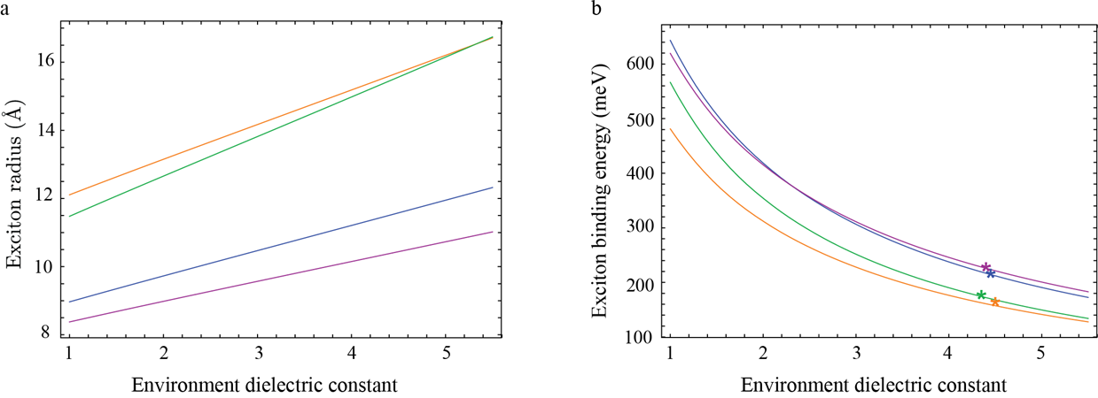
Figure 2: Variation of the exciton radius (a) and binding energy (b) in ML TMDs with the environment average dielectric constant. The orange lines are for ML WSe₂ ($\mu_{r}=0.2m_{0},r_{0}=45$ Å), green lines – for ML WS₂ ($\mu_{r}=0.175m_{0},r_{0}=34$ Å), blue lines – for ML MoS₂ ($\mu_{r}=0.275m_{0},r_{0}=34$ Å), and purple lines – for ML MoSe₂ ($\mu_{r}=0.35m_{0},r_{0}=39$ Å). The small stars with the respective colors depict the corresponding experimental amounts for $E_{b}$.³³

From here, one can find the exciton radius as the variational parameter and the corresponding exciton binding energy for any set of input variables, including exciton mass $\mu_{r}$ and dielectric characteristics $r_{0}$ and $\kappa$. Unlike $\mu_{r}$ and $r_{0}$ as inherent features of an ML TMD, the environment average dielectric constant can be tuned by changing encapsulating materials above and below the ML. Thus Eq. (11) provides the possibility to adjust exciton binding energy and space extent, which is an advantage of ML TMDs compared to conventional 2D semiconductors. In the last, with the regular Coulomb carrier-carrier interaction, the exciton binding energy and radius are related to each other as $E_{b}a_{x}=e^{2}/\varepsilon_{0}\varepsilon$,⁵⁶ and the kinetic and electron-hole interaction energies equal $E_{b}$ and $-2E_{b}$, respectively, independent of the material. With the Keldysh potential, the electron-hole interaction energy can be regulated by tuning the potential strength, ceasing to be commensurate with $E_{b}$. The ratio between its absolute quantity and the kinetic energy considerably increases, depending on the mass and dielectric screening parameters. For freestanding ML TMDs, the ratio varies in the interval 4 – 5 in different ML TMDs, indicating the exciton robustness due to reduced screening. Naturally, excitons are stronger bound in a sample with shorter $r_{0}$ and an environment with smaller $\kappa$, wherein the Keldysh potential is more effective. As Eq. (11) shows, in the same dielectric screening conditions, heavier excitons with lesser kinetic energy are more robust with more binding energy and correspondingly smaller radius. We put in Figure 2 the variation of these exciton features with $\kappa$ in four ML TMDs, whose inherent chracteristics $\mu_{r}$ and $r_{0}$ are taken from experiments.^32,33 Experimentally, the reduction of the exciton size with environment screening is reported in ref. 57 and the increase of the exciton binding energy – ref 58. Moreover, Hsu et al. observe a close agreement of their findings with the description of the Keldysh potential.⁵⁸ As one sees from Fig. 2b, the Keldysh potential also gives for $E_{b}$ in hBN encapsulated ML TMDs the amounts close to experimental ones, though with slight underestimates.^32,33

In the first nonlinear approximation, two-pair correlations give rise to the exciton-exciton interaction. They are mediated by the interaction terms in Hamiltonian (6) with interacting carriers belonging to two different electron-hole pairs. We show these correlations in detail in the Supplementary Note, where one can see the mechanism of various components of the exciton-exciton interaction. In particular, the interaction between identical bright excitons and between those from opposite valleys. As expected, the carrier-carrier interaction within a single valley mediates the correlations leading to the interaction between excitons in this valley. Meanwhile, as one can see from Supplementary Fig. 2, the intervalley exciton-exciton coupling is induced not only by the intervalley carrier-carrier interactions of all types, but also by the intravalley electron-hole interactions. As a result, we obtain a Hamiltonian of the effective exciton-exciton interaction in the form,

$$\mathcal{H}_{x-x} = \frac{1}{2S}\sum\limits_{\mathbf{\mathcal{K}}_{1},\mathbf{\mathcal{K}}_{2},\mathbf{Q}}\left\{\sum\limits_{\Gamma}\left[U^{d}(\mathbf{Q})+U^{ex}(\mathbf{\mathcal{K}},\mathbf{Q})\right]A_{\Gamma,\mathbf{\mathcal{K}}_{1}+\mathbf{Q}}^{+}A_{\Gamma,\mathbf{\mathcal{K}}_{2}-\mathbf{Q}}^{+}A_{\Gamma,\mathbf{\mathcal{K}}_{2}}A_{\Gamma,\mathbf{\mathcal{K}}_{1}}\right.$$ (12)

$$+2\sum\limits_{\begin{subarray}{c}\Gamma=\Gamma_{2},\Gamma_{3}\\ \Gamma^{\prime}=\Gamma_{5},\Gamma_{6}\end{subarray}}\left[U^{d}(\mathbf{Q})+U^{ex}(\mathbf{\mathcal{K}},\mathbf{Q})\right]A_{\Gamma,\mathbf{\mathcal{K}}_{1}+\mathbf{Q}}^{+}A_{\Gamma^{\prime},\mathbf{\mathcal{K}}_{2}-\mathbf{Q}}^{+}A_{\Gamma^{\prime},\mathbf{\mathcal{K}}_{2}}A_{\Gamma,\mathbf{\mathcal{K}}_{1}}$$

$$+2U^{d}(\mathbf{Q})\left[A_{\Gamma_{2},\mathbf{\mathcal{K}}_{1}+\mathbf{Q}}^{+}A_{\Gamma_{3},\mathbf{\mathcal{K}}_{2}-\mathbf{Q}}^{+}A_{\Gamma_{3},\mathbf{\mathcal{K}}_{2}}A_{\Gamma_{2},\mathbf{\mathcal{K}}_{1}}+A_{\Gamma_{5},\mathbf{\mathcal{K}}_{1}+\mathbf{Q}}^{+}A_{\Gamma_{6},\mathbf{\mathcal{K}}_{2}-\mathbf{Q}}^{+}A_{\Gamma_{6},\mathbf{\mathcal{K}}_{2}}A_{\Gamma_{5},\mathbf{\mathcal{K}}_{1}}\right]$$

$$-\left.2U^{ex}(\mathbf{\mathcal{K}},\mathbf{Q})\left[A_{\Gamma_{2},\mathbf{\mathcal{K}}_{1}+\mathbf{Q}}^{+}A_{\Gamma_{3},\mathbf{\mathcal{K}}_{2}-\mathbf{Q}}^{+}A_{\Gamma_{6},\mathbf{\mathcal{K}}_{2}}A_{\Gamma_{5},\mathbf{\mathcal{K}}_{1}}+A_{\Gamma_{5},\mathbf{\mathcal{K}}_{1}+\mathbf{Q}}^{+}A_{\Gamma_{6},\mathbf{\mathcal{K}}_{2}-\mathbf{Q}}^{+}A_{\Gamma_{3},\mathbf{\mathcal{K}}_{2}}A_{\Gamma_{2},\mathbf{\mathcal{K}}_{1}}\right]\right\},$$

where $U^{d}(\mathbf{Q})$ and $U^{ex}(\mathbf{\mathcal{K}},\mathbf{Q})$ ($\mathbf{\mathcal{K}}=\mathbf{\mathcal{K}}_{1}-\mathbf{\mathcal{K}}_{2}$) denote the direct and exchange interaction energy densities. They are functions of the Keldysh potential and four envelope functions of two interacting excitons before and after the interaction,

$$U^{d}\left(\mathbf{Q}\right) = \frac{V_{\mathbf{Q}}}{S^{2}}\left\{\sum_{\mathbf{p}_{1}}\digamma\left(\mathbf{p}_{1}+\alpha\mathbf{Q}\right)\digamma(\mathbf{p}_{1})^{\ast}\sum_{\mathbf{p}_{2}}\digamma\left(\mathbf{p}_{2}-\alpha\mathbf{Q}\right)\digamma\left(\mathbf{p}_{2}\right)^{\ast}\right.$$ (13)

$$+\sum_{\mathbf{p}_{1}}\digamma\left(\mathbf{p}_{1}-\beta\mathbf{Q}\right)\digamma(\mathbf{p}_{1})^{\ast}\sum_{\mathbf{p}_{2}}\digamma\left(\mathbf{p}_{2}+\beta\mathbf{Q}\right)\digamma\left(\mathbf{p}_{2}\right)^{\ast}$$

$$\left.-2\sum_{\mathbf{p}_{1}}\digamma\left(\mathbf{p}_{1}+\alpha\mathbf{Q}\right)\digamma(\mathbf{p}_{1})^{\ast}\sum_{\mathbf{p}_{2}}\digamma\left(\mathbf{p}_{2}+\beta\mathbf{Q}\right)\digamma\left(\mathbf{p}_{2}\right)^{\ast}\right\},$$

$$U^{ex}\left(\mathbf{\mathcal{K}},\mathbf{Q}\right) = -\frac{1}{S^{2}}\sum\limits_{\mathbf{p}_{1},\,\mathbf{p}_{2}}V_{p_{1}}\left\{\digamma\left(\mathbf{p}_{2}+\alpha\mathbf{Q}\right)\digamma\left(\mathbf{p}_{2}\right)^{\ast}\right.$$ (14)

$$\times\digamma\left(\mathbf{p}_{2}-\mathbf{p}_{1}+\beta\mathbf{\mathcal{K+}}\beta\mathbf{Q}\right)\,\digamma\left(\mathbf{p}_{2}-\mathbf{p}_{1}+\beta\mathbf{\mathcal{K+}Q}\right)^{\ast}$$

$$+\digamma\left(\mathbf{p}_{2}-\beta\mathbf{Q}\right)\digamma\left(\mathbf{p}_{2}\right)^{\ast}\digamma\left(\mathbf{p}_{2}-\mathbf{p}_{1}-\alpha\mathbf{\mathcal{K}}-\alpha\mathbf{Q}\right)\digamma\left(\mathbf{p}_{2}-\mathbf{p}_{1}-\alpha\mathbf{\mathcal{K-}Q}\right)^{\ast}$$

$$-2\digamma\left(\mathbf{p}_{2}-\mathbf{p}_{1}+\alpha\mathbf{Q}\right)\digamma\left(\mathbf{p}_{2}\right)^{\ast}$$

$$\left.\times\digamma\left(\mathbf{p}_{2}-\mathbf{p}_{1}+\beta\mathbf{\mathcal{K+}}\beta\mathbf{Q}\right)\,\digamma\left(\mathbf{p}_{2}-\mathbf{p}_{1}+\beta\mathbf{\mathcal{K+}Q}\right)^{\ast}\right\}.$$

The first, second, and last terms in braces on the right hand side (rhs) of these equations stand for the energy density of the direct [Eq. (13)] and exchange [Eq. (14)] exciton-exciton interaction induced by the electron-electron, hole-hole, and electron-hole interaction, respectively. The opposite sign of $U^{ex}$ is caused by the exchange of two carriers-fermions belonging to two interacting excitons. In the case of the intervalley interaction between the bright excitons, the respective terms are visualized in Supplementary Fig. 2. Equation (12) formulates the whole picture of the pairwise interaction between diverse excitons in the model under consideration, including three types. That is the interaction between identical excitons, between bright and dark excitons, and between bright excitons from opposite valleys, presented respectively by the first sum, second sum, and the last two terms in the braces in rhs of the equation. It is worth noting that only in terms of excitons valley momenta $\mathcal{H}_{x-x}$ has such a relatively compact form as Eqs. (12) – (14). In terms of their crystal momenta, each term of $\mathcal{H}_{x-x}$ has its respective form with the corresponding $U^{d}(\mathbf{Q})$ and $U^{ex}(\mathbf{\mathcal{K}},\mathbf{Q})$ [see Supplementary Eqs. (6) – (10)]. Equation (13) shows that the direct interaction disappears in the limit of small momentum transfer and the case of equal electron and hole masses. Therefore this part matters only at relatively far distances and when one of the exciton constituents is much heavier than the other. In ML TMDs, the electron and hole masses are comparable,^19,30,36,37 so we will put $\alpha\simeq\beta\simeq 1/2$ and consider the exciton-exciton interaction exclusively of the exchange nature. Description of the exchange exciton-exciton interaction is a problematic issue because of its nonlocality.⁵² We will draw the interaction’s qualitative features from basic symmetry principles and perform an approximate quantitative analysis relying on calculations for limiting cases. As a result of the Pauli exclusion principle, the exchange exciton-exciton interaction is short-range, repulsive between identical excitons and between bright and dark ones. We see from Supplementary Fig. 1 that a correlated structure of two identical (or one bright and one dark) excitons incorporate two (or one) couples of indistinguishable carriers-fermions. The last repel each other at distances, where their wave functions overlap,⁵⁹ resulting in a repulsive interaction between excitons. Meantime, Supplementary Fig. 2 shows that all carriers are distinguishable in a two-exciton structure incorporating different bright excitons, which can be on equal terms presented as a pair of dark ones. As $\Gamma_{2}\otimes\Gamma_{3}=\Gamma_{5}\otimes\Gamma_{6}=\Gamma_{1}$, such a structure is symmetric corresponding to the zero spin. Symmetric configurations are known to produce attractive forces.⁵⁹ Identical carriers in these structures have opposite spins compensating each other to the total spin 0, so the attraction is analogous to a chemical valence bond.³⁴

Thus, the exciton-exciton interaction in ML TMDs shares the same dependence on the interacting excitons’ symmetry, or spin, as in 2D or 3D conventional semiconductors with two simple bands and dipole allowed interband transition.^49-51 It is repulsive in all symmetry combinations of interacting excitons except for the case they together form a fully symmetric two-exciton structure (with total spin 0) when the interaction is attractive. As to the bright excitons, their interaction is repulsive for parallel spins and attractive for opposite ones.⁴⁹

Intravalley and intervalley exciton interaction potentials

Let us take a closer look at the intravalley and intervalley interaction energy. Consider first energy $E_{xx}\left(\Gamma_{2},\mathbf{\mathcal{K}}_{1},\mathbf{\mathcal{K}}_{2}\right)$ of two correlated bright $\Gamma_{2}$ excitons with momenta $\mathbf{\mathcal{K}}_{1}$ and $\mathbf{\mathcal{K}}_{2}$ in a structure of the type depicted in Supplementary Fig. 1a, d. Presenting the structure in the zeroth order approximation simply as $A_{\Gamma_{2},\mathbf{\mathcal{K}}_{1}}^{+}A_{\Gamma_{2},\mathbf{\mathcal{K}}_{2}}^{+}|\,\mathbf{0\,)}\diagup\sqrt{2}$, we get the average of the exciton Hamiltonian $\mathcal{H}_{x}=\sum\limits_{\Gamma,\,\mathbf{\mathcal{K}}}E_{x}(\Gamma,\mathbf{\mathcal{K}})A_{\Gamma,\,\mathbf{\mathcal{K}}}^{+}\,A_{\Gamma,\,\mathbf{\mathcal{K}}}+\mathcal{H}_{x-x}$ over it in the form of the sum of energies of two excitons and of their interaction, $E_{x}\left(\Gamma_{2},\mathbf{\mathcal{K}}_{1}\right)+E_{x}\left(\Gamma_{2},\mathbf{\mathcal{K}}_{2}\right)+\left[U_{\Gamma_{2}-\Gamma_{2}}^{ex}(\mathbf{\mathcal{K}},0)+U_{\Gamma_{2}-\Gamma_{2}}^{ex}(\mathbf{\mathcal{K}},-\mathbf{\mathcal{K}})\right]\diagup 2S$. In the expression for $U_{\Gamma_{2}-\Gamma_{2}}^{ex}(\mathbf{\mathcal{K}},0)$ and $U_{\Gamma_{2}-\Gamma_{2}}^{ex}(\mathbf{\mathcal{K}},-\mathbf{\mathcal{K}})$ in terms of excitons’ crystal momenta [see Supplementary Eq. (7)], in the place of Fourier images $V_{k}$ of the Keldysh potential and of exciton wave functions we insert their Fourier transformations by definition. After some elementary transfigurations, we get the integral representation of the intravalley interaction energy of two excitons with crystal momenta $\mathbf{k}_{1}$ and $\mathbf{k}_{2}$,

$$\frac{2}{S}\int\!d^{2}r\,\exp[i\alpha\mathbf{kr}]\int\!d^{2}r_{1}\,f(r_{1})\,f\left(\left|\mathbf{r}_{1}+\mathbf{r}\right|\right)$$ (15)

$$\times\int\!d^{2}r_{2}\,\,f(r_{2})\,f\left(\left|\mathbf{r}_{2}-\mathbf{r}\right|\right)\left\{V_{K}\left(\left|\mathbf{r}_{2}-\mathbf{r}\right|\right)-V_{K}\left(r\right)\right\}$$

$$\equiv \frac{1}{S}\int\!d^{2}r\,\exp[i\mathbf{kr}]\,\mathcal{U}_{\Gamma-\Gamma}(r)$$

where $\mathbf{k\equiv k}_{1}-\mathbf{k}_{2}$. Function of distance $\mathcal{U}_{\Gamma-\Gamma}(r)$ ($\Gamma=\Gamma_{2},\Gamma_{3}$) defines the intravalley interaction potential between identical bright excitons in the limit of vanishing momentum transfer. For $\mathbf{k}=0$, the integral of $\mathcal{U}_{\Gamma-\Gamma}(r)$ over 2D space gives us the intravalley interaction energy in the limit of equal momenta of interacting excitons, $U_{{}_{\Gamma-\Gamma}}^{ex}(0,0)\equiv U_{{}_{\Gamma-\Gamma}}^{ex}$ ($\Gamma=\Gamma_{2},\Gamma_{3}$). Independent of the valley position, $\mathcal{U}_{\Gamma-\Gamma}(r)$ is closely similar to its counterpart in conventional semiconductors: each of its terms is a product of two two-center integrals met in theory of diatomic molecules.^52,60 The difference is, the carrier-carrier interaction has the form of the Keldysh potential and the consequent exciton wave function is a variational one instead of the hydrogenic function.

As to the intervalley interaction energy of different bright excitons, let us present a symmetric two-exciton structure of the type in Supplementary Fig. 2 in the form $\left[A_{\Gamma_{2},\mathbf{\mathcal{K}}_{1}}^{+}A_{\Gamma_{3},\mathbf{\mathcal{K}}_{2}}^{+}+A_{\Gamma_{5},\mathbf{\mathcal{K}}_{1}}^{+}A_{\Gamma_{6},\mathbf{\mathcal{K}}_{2}}^{+}\right]|\,\mathbf{0\,)}\diagup\sqrt{2}$, which diagonalizes the exciton Hamiltonian average. In terms of excitons’ crystal momenta [see Supplementary Eqs. (9), (10)], the structure energy has the form

$$E_{x}\left(k_{1}\right)+E_{x}\left(k_{2}\right)-\frac{2}{S}U_{\Gamma_{2}-\Gamma_{3}}^{ex}(\mathbf{k},0)$$

$$+E_{x}\left(\mathbf{k}_{1}+\mathbf{K-K}^{\prime}\right)+E_{x}\left(\mathbf{k}_{2}+\mathbf{K}^{\prime}\mathbf{-K}\right)-\frac{2}{S}U_{\Gamma_{5}-\Gamma_{6}}^{ex}(\mathbf{k}+2\mathbf{K}-2\mathbf{K}^{\prime},0)$$ (16)

where the excitons intervalley interaction energy reads

$$\frac{1}{S}U_{\Gamma_{2}-\Gamma_{3}}^{ex}(\mathbf{k},0) = \frac{1}{S}U_{\Gamma_{5}-\Gamma_{6}}^{ex}(\mathbf{k},0)^{\ast}$$ (17)

$$= \frac{2}{S}\int\!d^{2}r\,\exp[i\alpha\mathbf{kr}]\int\int\!d^{2}r_{1}d^{2}r_{2}\exp\left[i\alpha\left(\mathbf{K-K}^{\prime}\right)\left(\mathbf{r}_{1}-\mathbf{r}_{2}\right)\right]$$

$$\times f(r_{1})\,f(|\mathbf{r}_{1}+\mathbf{r}|)\,f(r_{2})\,f(|\mathbf{r}_{2}-\mathbf{r}|)\left[V_{K}\left(|\mathbf{r}_{2}-\mathbf{r}|\right)-V_{K}(r)\right]$$

$$\equiv -\frac{1}{S}\int\!d^{2}r\,\exp[i\mathbf{kr}]\,\mathcal{U}_{\Gamma_{2}-\Gamma_{3}}(r)$$

Here $\mathcal{U}_{\Gamma_{2}-\Gamma_{3}}(r)$ is an attractive interaction potential that outlines the interaction potential between $\Gamma_{2}$ and $\Gamma_{3}$ excitons in the limit of vanishing momentum transfer. Similarly to $U_{{}_{\Gamma-\Gamma}}^{ex}$ ($\Gamma=\Gamma_{2},\Gamma_{3}$), we quantify the intervalley interaction potential by the value of the integral of $\left|\mathcal{U}_{\Gamma_{2}-\Gamma_{3}}(r)\right|$ over 2D space that we denote by $U_{\Gamma_{2}-\Gamma_{3}}^{ex}$. We will refer to the quantity as the intervalley interaction energy (in the limit of equal momenta). Comparing Eqs. (17) and (15) we see that the interaction between distant $\Gamma_{2}$ and $\Gamma_{3}$ excitons in the momentum space is described by an oscillating exponent in the inner two-center integrals (over $\mathbf{r}_{1}$ and $\mathbf{r}_{2}$). From Eq. (5) and the form of the exciton wave function, we have the oscillation frequency $2\pi/(3\sqrt{3})a_{x}/a$, which roughly varies between 3.5 and 6.5 for $a\sim 3$ Å and $a_{x}$ in the range $9-17$ Å (see Fig. 2a). Consequently, the intervalley interaction potential is much weaker compared to its intravalley counterpart. Essentially, the potential depends substantially on the exciton extent defining the overlap degree of the wave functions of interacting excitons from $K$ and $K^{\prime}$ valleys in the momentum space. As expected, the smaller the exciton radius (the more extended the exciton wave function $\digamma(\mathbf{k})$) is, the stronger the intervalley interaction potential.

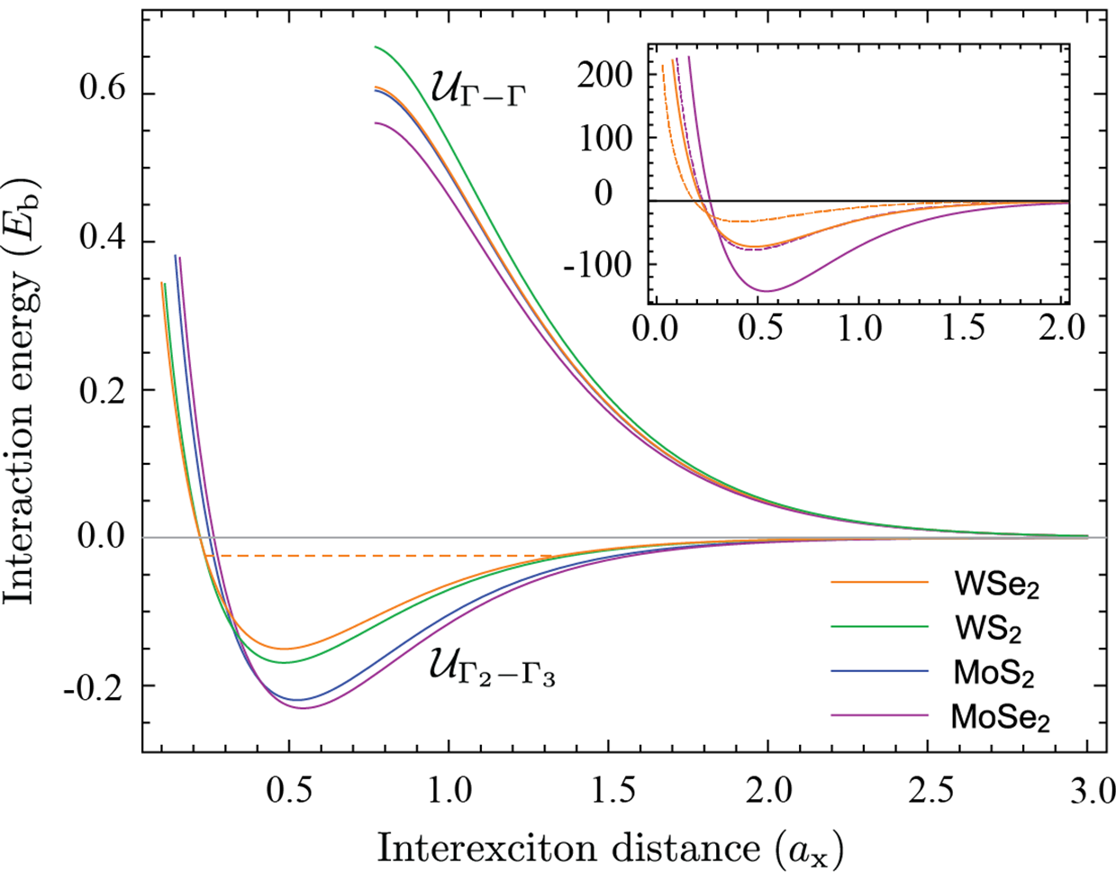
Figure 3: Intravalley $\mathcal{U}_{\Gamma-\Gamma}$ ($\Gamma=\Gamma_{2},\Gamma_{3}$) and intervalley exciton interaction potential $\mathcal{U}_{\Gamma_{2}-\Gamma_{3}}$ in the limit of vanishing momentum transfer in different freestanding ML TMDs. The dashed line inside the intervalley potential in ML WSe₂ depicts the approximate position of the intervalley biexciton energy. We put lattice constant $a=3.3$ Å for ML MoSe₂ and WSe₂, and $a=3.2$ Å for ML MoS₂ and WS₂.³⁷ Inset: The intervalley interaction potential in ML MoSe₂ and WSe₂ in vacuum (solid lines) and hBN encapsulation (dashed lines) in the unit of millielectronvolt.

With the particular experimental value of $\mu_{r}$ and $r_{0}$ for different ML TMDs,³³ the exciton radius, binding energy, and interaction energies $U_{\Gamma-\Gamma}^{ex}$ and $U_{\Gamma_{2}-\Gamma_{3}}^{ex}$ obtained for freestanding ML TMDs are shown in the upper part of Table 1, and potentials $\mathcal{U}_{\Gamma-\Gamma}(r)$ and $\mathcal{U}_{\Gamma_{2}-\Gamma_{3}}(r)$ as functions of relative distance $r/a_{x}$ – in Fig. 3. The interaction potentials (energies) computed for a ML TMD are expressed in the unit of $E_{b}$ ($E_{b}a_{x}^{2}$) found for the material. As the electron-hole interaction energy [see Eq. (11)], the intravalley interaction potential in its absolute quantity weakens with increasing ratio $r_{0}/\kappa a_{x}$. For $\kappa=1$ this trend is seen from amounts of $r_{0},a_{x}$ and $U_{{}_{\Gamma-\Gamma}}^{ex}$ in the upper part of Table 1 and Fig. 3. Meanwhile, the potential shape remains the same for all ML TMDs with a repulsive wall at small distances and an exponential fall at larger ones. These features are characteristic of the interaction between excitons,^52,60 resembling that between atoms in diatomic molecules.³⁴ Further, for freestanding ML TMDs, the intravalley interaction strength is somewhat above $2E_{b}\,a_{x}^{2}$. On the scale $\sim 2E_{b}\,a_{x}^{2}$ it has been guesstimated in ref. 9 for ML WS₂. If in Eq. (15) replace $V_{K}(r)$ by the Coulomb potential, the integral gives the known result $U^{ex}|_{C}=8\pi E_{b}\,a_{x}^{2}\left(1-315\pi^{2}/2^{12}\right)\approx 6E_{b}\,a_{x}^{2}$.^48,51 Thus, reduced screening makes the relative exciton-exciton interaction energy nearly thrice less compared to its amount in the limit of Coulomb potential $V_{C}(r)$. The exciton-exciton interaction terms mediated respectively by the electron-hole, electron-electron, and hole-hole interactions become more with the reduced screening. However, their magnitudes are closer to each other, so their difference decreases, involving lesser exciton-exciton interaction relative to the exciton binding energy. The result means high stability of valley excitons relative to their pairwise interaction and a wide valid range of the low-density limit. We should note that as $E_{b}$ in ML TMDs is by orders more than in conventional semiconductors, in its absolute quantity, the exciton-exciton interaction in the former is enhanced, compared to that in the latter.^9,24

Table 1: Experimental values of input variables in different ML TMDs and resultant calculated exciton binding energy and radius, intravalley and intervalley exciton interaction energies, and biexciton binding energy. Available appropriate experimental measurements of the exciton and biexciton binding energies are shown in parentheses for comparison.

	MoSe2	MoS2	WS2	WSe2
$\mu_{r}$ ($m_{0}$)33	0.350	0.275	0.175	0.200
$r_{0}$ (Å)33	39	34	34	45
		Freestanding
$E_{b}$ (meV)	620	644	566	481
$a_{x}$ (Å)	8.38	8.96	11.48	12.11
$U_{\Gamma-\Gamma}^{ex}$ ($E_{b}a_{x}^{2}$)	2.043	2.173	2.341	2.187
$U_{\Gamma_{2}-\Gamma_{3}}^{ex}$ ($E_{b}a_{x}^{2}$)	0.952	0.863	0.602	0.539
$\mathcal{E}_{0}$ (meV)	64.9	53.4 (6012)	18.5	12.9
		hBN encapsulated
$\kappa^{33}$	4.4	4.45	4.35	4.5
$E_{b}$ (meV)	226 (23133)	215 (22133)	174 (18033)	157 (16732)
$a_{x}$ (Å)	10.38	11.53	15.39	15.69
$U_{\Gamma-\Gamma}^{ex}$ ($E_{b}a_{x}^{2}$)	3.355	3.584	3.826	3.620
$U_{\Gamma_{2}-\Gamma_{3}}^{ex}$ ($E_{b}a_{x}^{2}$)	1.177	0.996	0.642	0.615
$\mathcal{E}_{0}$ (meV)	24.0 (2127)	13.2	1.5	1.4 (16 – 1718)

As to the intervalley interaction, the weakening with increasing exciton size can be seen from Table 1 and Fig. 3. The intervalley interaction energy $U_{\Gamma_{2}-\Gamma_{3}}^{ex}$ is one half of the intravalley counterpart $U_{\Gamma-\Gamma}^{ex}$ in freestanding ML MoSe₂ with the smallest exciton, but just a fourth of $U_{\Gamma-\Gamma}^{ex}$ in ML WSe₂ with the largest one. Figure 3 shows that $\mathcal{U}_{\Gamma_{2}-\Gamma_{3}}(r)$ is very short-range with its depth increasing with the decrease of $a_{x}$. Meantime, the potential width $a_{w}$ (width at half minimum) decreases in absolute quantity remaining in a narrow interval $0.65a_{x}-0.67a_{x}$ in freestanding ML TMDs. In the presence of environment dielectric screening, the potential width increases with $a_{x}$ in absolute quantity though it slightly decreases in the unit of $a_{x}$. Examinations show that even for the most strong potential $\mathcal{U}_{\Gamma_{2}-\Gamma_{3}}^{m}(r)$ in freestanding ML MoSe₂, its average value (the value at half minimum) meets the inequality $\left|\overline{\mathcal{U}_{\Gamma_{2}-\Gamma_{3}}^{m}(r)}\right|\ll 2\diagup\mu_{x}a_{w}^{2}$. Thus for any possible value of the input variables, the intervalley interaction potential can be considered as a perturbation³⁴ to the free relative motion of $\Gamma_{2}$ and $\Gamma_{3}$ excitons in their correlated symmetric structures. Clearly, the shallower the potential is, the better the perturbation criterion is fulfilled. To the detail, the criterion inequality corresponds to the ratio of 1 to 5, 1 to 6, and 1 to 9 for freestanding ML MoSe₂, MoS₂, and both members of MoX₂ subgroup, respectively, while in an hBN encapsulation it is correspondingly 1 to 7, 1 to 8, and 1 to 14.

Intervalley biexciton

Let us consider a superposition of correlated symmetric structures of two bright excitons from opposite valleys having a definite valley momentum $\mathbf{\mathcal{P}}$

$$|\Gamma_{1},\mathbf{\mathcal{P}}\,) = \frac{1}{\sqrt{2S}}\sum\limits_{\mathbf{\mathcal{K}}}\Psi(\mathbf{\mathcal{K}})\left[A_{\Gamma_{2},\,\mathbf{\mathcal{K}+\mathcal{P}}/2\,}^{+}A_{\Gamma_{3},\mathbf{-\mathcal{K}+\mathcal{P}}/2}^{+}+A_{\Gamma_{5},\mathbf{\mathcal{K}+\mathcal{P}}/2\,}^{+}A_{\Gamma_{6},\mathbf{-\mathcal{K}+\mathcal{P}}/2}^{+}\right]\,|\,0\,)$$ (18)

$$\equiv B_{\mathbf{\mathcal{P}}}^{+}\,|\,0\,)$$

It is straightforward to examine, that this two-exciton entity, whose valley momentum equals its crystal momentum, is an eigenstate of Hamiltonian $\mathcal{H}_{x}$ of the exciton system with effective exciton-exciton interaction,

$$\mathcal{H}_{x}|\Gamma_{1},\mathbf{\mathcal{P}}\,)=E_{xx}(\mathcal{P})|\Gamma_{1},\mathbf{\mathcal{P}}\,)$$ (19)

with energy $E_{xx}(\mathbf{\mathcal{P}})=2E_{x}+\mathbf{\mathcal{P}}^{2}/4\mu_{x}+\mathcal{E}_{xx}$ and the envelope function $\Psi(\mathbf{\mathcal{K}})$ obeying the equation

$$\frac{\mathcal{K}^{2}}{\mu_{x}}\Psi(\mathbf{\mathcal{K}})-\frac{2}{S}\sum\limits_{\mathbf{\mathcal{Q}}}U_{\Gamma_{2}-\Gamma_{3}}^{ex}(2\mathbf{\mathcal{K}},\mathbf{\mathcal{Q}})\Psi(\mathbf{\mathcal{K}}+\mathbf{\mathcal{Q}})=\mathcal{E}_{xx}\Psi(\mathbf{\mathcal{K}})$$ (20)

We see, that $|\Gamma_{1},\mathbf{\mathcal{P}}\,)$ is a correlated two-exciton entity with total mass $2\mu_{x}$ and reduced mass $\mu_{x}/2$, whose energy includes the kinetic energy of its free motion as a whole and internal energy $\mathcal{E}_{xx}$ of the excitons relative motion in the field of their mutual attractive interaction. The internal energy is positive for the scattering states and negative for bound states with binding energy $\mathcal{E}_{b}=-\mathcal{E}_{b,xx}>0$. We call $|\Gamma_{1},\mathbf{\mathcal{P}}\,)$ the intervalley biexciton in the broad sense of the word though conventionally it is used to refer to the bound state only. As a nonlocal function of two vectors-variables, $U_{\Gamma_{2}-\Gamma_{3}}^{ex}(2\mathbf{\mathcal{K}},\mathbf{\mathcal{Q}})$ is presented in the real space by a nonlocal potential $\mathcal{U}_{\Gamma_{2}-\Gamma_{3}}(r,r^{\prime})^{60}$ and Eq. (20) is therefore an integrodifferential equation. It cannot be analyzed with usual methods of nonlinear dynamics and bound to be reduced by approximations. The approach proposed in ref. 52, which consists in expanding the exchange interaction energy density into a series of powers of $\alpha$, can be applied. However, with $\alpha\approx\beta\approx 1/2$, one has to retain a large number of the series terms yielding a high order differential equation. Dealing with such an approximate solution of Eq. (20) is itself a demanding issue that is beyond the scope of this paper. We note only that i) $\mathcal{U}_{\Gamma_{2}-\Gamma_{3}}(r)$ comes from the main zero-order term of the mentioned series, ii) the intervalley interaction energy is that of the real nonlocal potential, $U_{\Gamma_{2}-\Gamma_{3}}^{ex}=\int d^{2}r\left|\mathcal{U}_{\Gamma_{2}-\Gamma_{3}}(r)\right|=\int d^{2}r\,d^{2}r^{\prime}\left|\mathcal{U}_{\Gamma_{2}-\Gamma_{3}}(r,r^{\prime})\right|$, and iii) $\mathcal{U}_{\Gamma_{2}-\Gamma_{3}}(r)$ in combination with the first and second-order terms of the series corresponds to an equivalent energy-dependent local potential of the same range ($a_{w}$), which is slightly deeper with minimum shifted towards a larger distance. Therefore binding energy $\mathcal{E}_{0}$ of the bound state supported by $\mathcal{U}_{\Gamma_{2}-\Gamma_{3}}(r)$ can be considered a lower bound for the biexciton binding energy, i.e. the minimal amount $\mathcal{E}_{b}$ can have for a set of input variables values, $\mathcal{E}_{0}\lesssim\mathcal{E}_{b}$. Because we can acquire $\mathcal{E}_{0}$ just approximately as one can see later, it indicates a narrow range, wherein the biexciton binding energy might be. Thus we will refer to this quantity approximately as biexciton binding energy. Presenting the envelope function of the bound state as $\psi(\mathbf{r})=R(r)\exp[im\varphi]/2\pi$ with $m$ an integer, we have the equation for its radial part,

$$-\frac{1}{\mu_{x}}\frac{1}{r}\frac{d}{dr}\left[r\frac{d}{dr}R(r)\right]+\left[\mathcal{U}_{\Gamma_{2}-\Gamma_{3}}(r)+\frac{m^{2}}{\mu_{x}r^{2}}\right]R(r)=-\mathcal{E}_{0}\,R(r)$$ (21)

Detailed checking shows that already for $m=1$ the centrifugal term predominates in strength over $\mathcal{U}_{\Gamma_{2}-\Gamma_{3}}^{m}(r)$. Hence for any realistic amount of input parameters, Eq. (21) with a repulsive effective potential has no negative solution. Thus the intervalley interaction potential can support only bound states with $m=0$. Moreover, our calculations using Eq. (30) in ref. 61 for the number of such bound states in a 2D potential show that for realistic amounts of the input parameters, $\mathcal{U}_{\Gamma_{2}-\Gamma_{3}}(r)$ can host only one bound state. Its binding energy can be estimated in a perturbation theory manner as shown by Landau and Lifshitz,³⁴

$$\mathcal{E}_{0}\sim\frac{2}{\mu_{x}a_{w}^{2}}\exp\left\{-\frac{2}{\mu_{x}}\frac{2\pi}{U_{\Gamma_{2}-\Gamma_{3}}^{ex}}\right\}$$ (22)

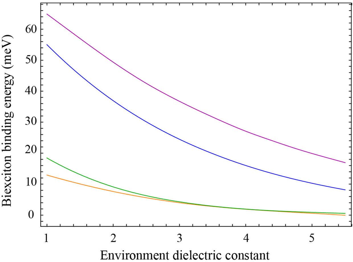
Figure 4: Variation of the intervalley biexciton binding energy with environment screening in four ML TMDs. The lines come from the interpolation between multiple points calculated with the use of Eqs. (22) and (17). As in Figs. 2 and 3, the orange line is for ML WSe₂, green line – ML WS₂, blue line – ML MoS₂, and purple line – ML MoSe₂.

We see an exponential increase of the biexciton binding energy with the exciton mass and intervalley interaction energy $U_{\Gamma_{2}-\Gamma_{3}}^{ex}$ that itself rises with increasing mass and decreasing screening. Consequently, $\mathcal{E}_{0}$ is sensitive to any variation of the input variables, which might help explaining disagreement between the reported experimental measurements.^11-18 The sensitivity is most relevant to the exciton mass, which enters the exponent’s degree in Eq. (22), and is one of the variables determining $U_{\Gamma_{2}-\Gamma_{3}}^{ex}$. Therefore the biexciton binding energy in ML MoX₂ with heavier excitons is much more than in ML WX₂. One can see from Table 1 that the ratio between the amounts of $\mathcal{E}_{0}$ in two groups is several times in freestanding samples. We note that the number we obtain for freestanding ML MoS₂ is near the measurement of Sie et al.¹² To our knowledge, experimental data of the biexciton binding energy in remaining ML TMDs in a vacuum is not available. As to the other inherent parameter, the dependence of $\mathcal{E}_{0}$ on $r_{0}$ is through $a_{x}$, whereon $U_{\Gamma_{2}-\Gamma_{3}}^{ex}$ strongly depends. We see from Fig. 2a that in any environment, the exciton is largest in ML WSe₂ with longest $r_{0}$, though $\mu_{r}$ in ML WS₂ is a little lighter. The exciton extent determines the intervalley interaction strength, so the biexciton binding energy in ML WSe₂ is least, as seen from Fig. 4, where we put the variation of $\mathcal{E}_{0}$ with $\kappa$ in all four ML TMDs. In light of our results for ML WS₂ and WSe₂ shown in the figure, it is unlikely the intervalley biexciton binding energy in the range of 45–65 meV, which has been deduced from observed resonances in early experiments on SiO₂ substrated ML WSe₂ and WS₂.^13-15 Doubts have been raised recently about the nature of those resonances with different mechanisms suggested for their origin.^8.62 As one can see from Fig. 1, in ML WX₂ the energy of the spin-dark excitons is below that of the bright ones. Therefore the part of their optical spectra below the exciton resonance is much richer than in ML MoX₂. The physical origin of different experimentally observed peaks in the low-energy part of spectra of ML WX₂ is still not clear,⁸ so their misinterpretation seems a common practice. Encapsulation by hBN flakes often used lately^7,27,32,33 considerably improves the spectra by reducing excitonic linewidths to $\sim$ 2–4 meV at 4 K [7]. The marked increase of $a_{x}$ at $\kappa\sim 4.5$ (see Table 1) leads to a sharp decline of the intervalley interaction (see Fig. 3, the Inset) involving a striking decrease of the biexciton binding energy. We find that $\mathcal{E}_{0}$ goes down to the range of 24 meV in hBN encapsulated ML MoSe₂, which agrees with the recent measurement of Yong et al.²⁷ In hBN encapsulated ML WX₂, the exciton radius becomes about five times larger than the lattice constant. The oscillating factor with a frequency of about 6 in rhs of Eq. (17) severely diminishes the intervalley interaction potential. Quantum mechanically speaking, the exciton wave functions at the $K$ and $K^{\prime}$ valleys become so small and localized in the momentum space that they can hardly overlap. As a result, $\mathcal{E}_{0}$ dramatically falls off to values less than excitonic linewidths. In this connection, an amount in the range 16–17 meV reported for the biexciton binding energy in hBN encapsulated ML WSe₂ [18] appears to be a misinterpretation. It is not convincing that the authors claim about the agreement of their measurement with those of refs. 16 and 17, and also with theoretical results of refs. 19–22. First, experiments in refs. 16 and 17 are on sapphire substrates, and in the latter, the sample is ML MoSe₂. Taking high-frequency dielectric constant of sapphire substrates $\varepsilon_{b}=9.3$,⁶³ we get numbers about 19 meV and 0.4 meV for $\mathcal{E}_{0}$ in ML MoSe₂ and WSe₂, respectively. The former agrees with the experimental measurement of Hao et al.,¹⁶ giving another example, that Eq. (22) provides reasonable judgment of $\mathcal{E}_{0}$ in ML MoX₂. Meantime, the obtained number for ML WSe₂ is even smaller than the smallest ($3\pm 0.5$ meV), not mentioning the largest ($18\pm 0.5$ meV), among three values for $\mathcal{E}_{0}$ the authors of ref. 17 infer from their time-resolved differential absorption data. For $\kappa\approx 5.15$, potential $\mathcal{U}_{\Gamma_{2}-\Gamma_{3}}(r)$ is still shallower than it is in the case of $\kappa=4.5$ shown in the Inset of Fig. 3, with an average value of about $-15$ meV. The potential fine meets the perturbation criterion, so estimation by Eq. 22 is credible.

Concerning theoretical works on the biexciton,^19-23 we should note the following. The starting intervalley biexciton model in these works is the same as ours. That is a 2D two-pair structure with indentical carriers having opposite spins and the Keldysh carrier-carrier interaction. However, the fact that the two electron-hole pairs forming the intervalley biexciton come from different edges of BZ has not been taken into consideration. Besides, the exchange interaction that is the primary part of the interaction between excitons has been coped with inadequately. Further, with the Keldysh carrier-carrier interaction, the relationship between the exciton binding energy and radius is determined by its reduced mass and dielectric parameters, as described by Eq. (11). By assuming the hydrogenic model relationship $E_{b}a_{x}=e^{2}/\varepsilon_{0}\varepsilon$, the authors exclude the exciton mass from their examinations. As a result, their biexciton binding energy depends only on the screening length and electron-hole mass ratio. With values of the last differing not much, the obtained amounts for $\mathcal{E}_{0}$ in different ML TMDs are close to each other.^19-22 Overall, that seems the biexciton model considered in those works has little in common with the intervalley biexciton in a real ML TMD.

Undoubtedly, our theoretical model involving approximations contains inaccuracies, and the used experimental measurements of input parameters entail uncertainties. In connection with the sensitivity of the biexciton binding energy to the input variables, they might bring about considerable uncertainty of the result for $\mathcal{E}_{0}$. This concerns first the perturbation theory estimate in the form of Eq. (22). The better potential $\mathcal{U}_{\Gamma_{2}-\Gamma_{3}}(r)$ fulfills the perturbation criterion, the closer $\mathcal{E}_{0}$ is to the exact value. Details on the fulfillment in different ML TMDs listed earlier show that the approximation is good for the ML WX₂ in any environment and ML MoX₂ in the presence of environment screening. For freestanding ML MoSe₂, it is a rather crude approximation needing further improvement. Secondly, our model relies on the exciton effective mass description and Keldysh form of the carrier-carrier interaction leading to Eq. (11). By comparing the amount of $E_{b}$ following from the equation and its experimental value in hBN encapsulated ML TMDs (see Fig. 2b and Table 1, the lower part), we see that Eq. (11) slightly underestimates $E_{b}$, by 5 – 10 meV. The difference between the two amounts is most (about six percent) for ML WSe₂. By fitting Eq. (11) to 167 meV, we get either $\mu_{r}=0.21m_{0}$, taking into account the experimental uncertainty pointed out in ref. 32, and $r_{0}=42$ Å, or $\mu_{r}=0.22m_{0}$, as suggested by the authors’ group earlier in ref. 57, and $r_{0}=44$ Å. The two alternatives yield $\mathcal{E}_{0}$ approximately 19 meV in a vacuum and 2.5 meV in an hBN encapsulation. The relative change in both cases is sizeable, but in the latter, it does not change the fact that the biexciton is hard to observe in hBN encapsulated ML WSe₂, and in general, in an environment with $\kappa>3$ as one can see from Fig. 4. Thirdly, from Eq. (15) on, our computations are carried out for $\alpha=\beta$ yielding $U^{d}=0$. With the difference between electron and hole masses taken into consideration, the upper line in (16) gains an additional term $U^{d}(\mathbf{k}_{1}-\mathbf{k}_{2})$, which corresponds to a local potential $\mathcal{U}_{\Gamma_{2}-\Gamma_{3}}^{d}(r)$ in the coordinate space. The direct exciton interaction potential has a considerable positive value near $r\sim 0$,⁶⁰ then takes minor negative values adding an insignificant amount to potential $\mathcal{U}_{\Gamma_{2}-\Gamma_{3}}(r)$. As $\int d^{2}r\mathcal{U}_{\Gamma_{2}-\Gamma_{3}}^{d}(r)=U_{\Gamma_{2}-\Gamma_{3}}^{d}(0)=0$, it makes no contribution to intervalley interaction energy $U_{\Gamma_{2}-\Gamma_{3}}^{ex}$. In this way, with the little difference between $\mu_{e}$ and $\mu_{h}$ in ML TMDs,^19,30,36,37 neglecting the direct part of the exciton-exciton interaction is acceptable.

DISCUSSION

We have presented a theoretical model for the system of diverse ground state excitons in ML TMDs with their effective pairwise interaction in the low-density limit. We make use of a group theoretical classification scheme for the band states and related excitons, where each of them is notated by a one-dimensional irreducible representation of the Abelian group $C_{3h}$, the wave vector group at the $K$ and $K^{\prime}$ valleys. We limit ourselves to a simplified band structure of ML TMDs with a direct two-band scheme at each valley, yielding four exciton symmetry states, two bright and two dark ones. Analogous states the exciton has in conventional 2D and 3D semiconductors with twofold spin-degenerate bands and dipole-allowed interband transition. We find that qualitatively, excitons in ML TMDs interact with each other in the same way as their conventional counterparts. That is, the character of the interaction between excitons with $\Gamma$ and $\Gamma^{\prime}$ notations is defined by the product $\Gamma\otimes\Gamma^{\prime}$ representing the two-exciton correlated structure they together form. It is repulsive for $\Gamma\otimes\Gamma^{\prime}\neq\Gamma_{1}$, corresponding to a nonzero excitons total spin, and attractive in the only symmetric one, $\Gamma\otimes\Gamma^{\prime}=\Gamma_{1}$, corresponding to the spin $0$. Concerning the bright excitons, their mutual interaction is repulsive for parallel spins and attractive for opposite ones. The distinction of excitons and their pairwise interaction in ML TMDs is due to the materials’ particular band structure and reduced screening in the form of the Keldysh carrier-carrier interaction. The former drives excitons with opposite spins residing at inequivalent valleys distant in the momentum space. In this way, we find in ML TMDs the repulsive intravalley and attractive intervalley exciton-exciton interaction. The latter, naturally depending on the overlap degree of the exciton wave functions at two valleys, supports the intervalley biexciton formation. With the Keldysh form of the carrier-carrier interaction, the exciton radius determining the wave function extent is the variational parameter.

Quantitatively, we have established an analytical relationship of variational parameter $a_{x}$, and the corresponding exciton binding energy, with the exciton reduced mass and the sample and environment dielectric characteristics. The latter are thereby the input variables determining the former as primary features of the exciton, and also the exciton-exciton interaction and the intervalley biexciton binding energy. We have acquired the intervalley interaction potential as a function of the interexciton distance, showing its explicit dependence on the exciton radius. We find that for realistic values of the input variables, the intervalley interaction potential turns out to be sufficiently weak, permitting us to estimate biexciton binding energy $\mathcal{E}_{0}$ in a perturbation theory manner. In this way, we obtain its semianalytical dependence on the exciton mass and the sample and environment dielectric parameters. We notice that $\mathcal{E}_{0}$ is sensitive to every input variable, especially the exciton mass. We find that in a vacuum, $\mathcal{E}_{0}$ in molybdenum-based MLs with heavier excitons is several times larger than in tungsten-based ones, and the ratio rises to about an order in the presence of environment screening. The amounts of $\mathcal{E}_{0}$ we estimate for freestanding ML MoS₂, and also sapphire substrated and hBN encapsulated ML MoSe₂, well agree with available relevant experimental measurements. Meantime, our estimation for ML WSe₂ in those conditions gives values very small compared to two appropriate experimental reports. From our perspective, this might be connected with misclassifications of the observed experimental spectra.

The semianalytical relationship established between the exciton and biexciton binding energy with environment dielectric constant might be used for adjusting the exciton and biexciton feature of different ML TMDs in future optoelectronic applications. Further, from our symmetry-dependent exciton Hamiltonian, a system of Heisenberg equations of motion can be derived. Such a system would be a baseline for research on valley selective nonlinear effects in an ML TMD coherently driven near the exciton resonance. In this connection, it is worthwhile pointing out the applicability of the presented model. It describes the coherent dynamics dominating the initial stages of optical experiments⁶⁴ in the first nonlinear regime. Created exciton polarization has the phase of the exciting field, and its inherent part has not appeared yet. The interaction with the carriers, phonons, etc., available in the sample, whose concentration is assumed small, causes a weak dephasing of the exciton polarization resulting in a slight reduction of its coupling with field and an energy shift of the exciton resonance.⁴⁹ The model is inapplicable to conditions when the created exciton polarization becomes incoherent, or under an above gap excitation, when the resulting excited state population is a mixture of bound excitons and electron-hole plasma. The presence of excess carriers at a moderate density can considerably affect the exciton, its interaction with the light and each other.⁶⁵ At an intermediate density, the interaction of excitons with bound and unbound charged excitons (trions) can dress them into exciton-polarons.⁶⁶ However, the description of such effects is beyond the scope of the paper.

References

- (1) Mak K F, Lee C, Hone J, Shan J & Heinz T F. Atomically Thin MoS2: A New Direct-Gap Semiconductor. Phys. Rev. Lett. 105, 136805 (2010).
- (2) Splendiani, A. et al. Emerging Photoluminescence in Monolayer MoS2. Nano Lett. 10, 1271–1275 (2010).
- (3) Keldysh, L. V. Coulomb interaction in thin semiconductor and semimetal films. JETP Lett. 29, 658–661 (1979).
- (4) Wang, G. et al. Colloquium: excitons in atomically thin transition metal dichalcogenides. Rev. Mod. Phys. 90, 021001 (2018).
- (5) Mueller, T. & Malic, E. Exciton physics and device application of two-dimensional transition metal dichalcogenide semiconductors. NPJ 2D Mater. Appl. 2, 1–12 (2018).
- (6) Zhang, X.-X., You, Y., Zhao, S. Y. F. & Heinz, T. F. Experimental Evidence for Dark Excitons in Monolayer WSe2. Phys. Rev. Lett. 115, 257403 (2015).
- (7) Zhou, Y. et al. Probing dark excitons in atomically thin semiconductors via near-field coupling to surface plasmon polaritons. Nat. Nanotechnol. 12, 856–860 (2017).
- (8) Bao, D. et al. Probing momentum-indirect excitons by nearresonance photoluminescence excitation spectroscopy in WS2 monolayer. 2D Mater. 7 , 031002 (2020).
- (9) Shahnazaryan, V., Iorsh, I. V., Shelykh, I A. & Kyriienko, O. Exciton-exciton interaction in transition-metal dichalcogenide monolayers. Phys. Rev. B 96, 115409 (2017).
- (10) Erkensten, D., Brem, S. & Malic, E. Exciton-exciton interaction in transition metal dichalcogenide monolayers and van der Waals heterostructures. Phys. Rev. B 103, 045426 (2021).
- (11) Mai, C. et al. Many-Body Effects in Valleytronics: Direct Measurement of Valley Lifetimes in Single-Layer MoS2. Nano Lett. 14, 202–206 (2014).
- (12) Sie E J, Frenzel A J, Lee Y H, Kong J. & Gedik N. Intervalley biexcitons and many-body effects in monolayer MoS2. Phys. Rev. B 92, 125417 (2015)
- (13) You, Y. et al. Observation of biexcitons in monolayer WSe2. Nat. Phys. 11, 477–481 (2015).
- (14) Shang, J. et al. Observation of Excitonic Fine Structure in a 2D Transition-Metal Dichalcogenide Semiconductor. ACS Nano 9, 647–655 (2015).
- (15) Plechinger, G. et al. Identification of excitons, trions and biexcitons in single-layer WS2. Phys. Status Solidi Rapid Res. Lett. 9, 457–461 (2015).
- (16) Hao, K. et al. Neutral and charged inter-valley biexcitons in monolayer MoSe2. Nat. Commun. 8, 15552 (2017).
- (17) Steinhoff, A. et al. Biexciton fine structure in monolayer transition metal dichalcogenides. Nat. Phys. 14, 1199–1204 (2028).
- (18) Li, Z. et al. Revealing the biexciton and trion-exciton complexes in BN encapsulated WSe2. Nat. Commun. 9, 3719 (2018).
- (19) Kylänpää, I. and Komsa, H-P. Binding energies of exciton complexes in transition metal dichalcogenide monolayers and effect of dielectric environment. Phys. Rev. B 92, 205418 (2015).
- (20) Mayers. M. Z., Berkelbach, T. C., Hybertsen, M. S. & Reichman, D. R. Binding energies and spatial structures of small carrier complexes in monolayer transition-metal dichalcogenides via diffusion Monte Carlo. Phys. Rev. B 92, 161404 (2015).
- (21) Zhang, D. K., Kidd, D. W. & Varga, K. Excited Biexcitons in Transition Metal Dichalcogenides. Nano Lett. 15, 7002–7005 (2015).
- (22) Szyniszewski, M., Mostaani, E., Drummond, N. D. & Fal’ko, V. I. Binding energies of trions and biexcitons in two-dimensional semiconductors from diffusion quantum Monte Carlo calculations. Phys. Rev. B 95, 081301(R) (2017).
- (23) Mostaani, E. et al. Diffusion quantum Monte Carlo study of excitonic complexes in two-dimensional transition-metal dichalcogenides. Phys. Rev. B 96, 075431 (2017).
- (24) Stepanov, P. et al. Exciton-Exciton Interaction beyond the Hydrogenic Picture in a MoSe2 Monolayer in the Strong Light-Matter Coupling Regime. Phys. Rev. Lett. 126, 167401 (2021).
- (25) Cunningham, P. D., Hanbicki, A. T., Reinecke, T. L., McCreary, K. M. & Jonker, B. T. Resonant optical Stark effect in monolayer WS2. Nat Commun 10, 5539 (2019).
- (26) Sie, E. J. et al. Valley-selective optical Stark effect in monolayer WS2. Nat. Mater. 14, 290–294 (2015).
- (27) Yong, C.-K. et al. Biexcitonic optical Stark effects in monolayer molybdenum diselenide. Nat. Phys. 14, 1092–1096 (2018).
- (28) Kim, J. et al. Ultrafast generation of pseudo-magnetic field for valley excitons in WSe2 monolayers. Science 346, 1205–1208 (2014).
- (29) Ye, Z., Sun, D. & Heinz, T. F. Optical manipulation of valley pseudospin. Nat. Phys. 13, 26–29 (2017).
- (30) Berkelbach, T. C., Hybertsen, M. S. & Reichman, D. R. Theory of neutral and charged excitons in monolayer transition metal dichalcogenides. Phys. Rev. B 88, 045318 (2013).
- (31) Chernikov, A. et al. Exciton Binding Energy and Nonhydrogenic Rydberg Series in Monolayer WS2. Phys. Rev. Lett. 113, 076802 (2014).
- (32) Stier, A. V. et al. Magnetooptics of Exciton Rydberg States in a Monolayer Semiconductor. Phys. Rev. Lett. 120, 057405 (2018).
- (33) Goryca, M. et al. Revealing exciton masses and dielectric properties of monolayer semiconductors with high magnetic. Nat Commun 10, 4172 (2019).
- (34) Landau, L. D. & Lifshitz, E. M. Quantum Mechanics (Pergamon, New York, 1985) Secs. 45, 81.
- (35) Koster G F, Dimmock J O, Wheeler R G and Statz H. Properties of the Thirty–two Point Groups (MIT, Cambridge, 1963) ps. 59 – 62.
- (36) Liu, G. B., Xiao, D., Yao, Y., Xu, X. & Yao, W. Electronic structures and theoretical modelling of two-dimensional group-VIB transition metal dichalcogenides. Chem. Soc. Rev. 44, 2643–2663 (2015).
- (37) Kormanyos, A. et al. k.p theory for two-dimensional transition metal dichalcogenide semiconductors. 2D Mater. 2, 022001 (2015).
- (38) Glazov, M. M. et al. Spin and valley dynamics of excitons in transition metal dichalcogenide monolayers. Phys. Status Solidi (b) 252, 2349–2362 (2015).
- (39) Mandl, F. & Shaw, G. Quantum Field Theory (John Wiley & Sons, 2010).
- (40) Bir, G. L. & Pikus, G. E. Symmetry and Strain-induced Effects in Semiconductors (Wiley, New York, 1975) Sec. 19.
- (41) Xiao, D., Liu, G-B., Feng, W., Xu, X. & Yao, W. Coupled Spin and Valley Physics in Monolayers of MoS2 and Other Group-VI Dichalcogenides. Phys. Rev. Lett. 108, 196802 (2012).
- (42) Xu, X., Yao, W., Xiao, D. & Heinz, T. F. Spin and pseudospins in layered transition metal dichalcogenides Nat. Phys. 10, 343–350 (2014).
- (43) Kadanoff, L. P. & Baym, G. Quantum statistical mechanics (Benjamin Inc., New York, 1962).
- (44) Cudazzo, P., Tokatly, I. V. & Rubio, A. Dielectric screening in two-dimensional insulators: Implications for excitonic and impurity states in graphane. Phys. Rev. B 84, 085406 (2011).
- (45) Hanamura, E. & Haug, H. Condensation effects of excitons. Phys. Rep. 33, 209–284 (1977).
- (46) Castro Neto, A. H., Guinea, F., Peres, N. M. R., Novoselov, K. S. & Geim, A. K. The electronic properties of graphene. Rev. Mod. Phys. 81, 109–162
- (47) Wannier, G. H. The Structure of Electronic Excitation Levels in Insulating Crystals. Phys. Rev. 52, 191 (1937).
- (48) Tassone, F. & Yamamoto, Y. Exciton-exciton scattering dynamics in a semiconductor microcavity and stimulated scattering into polaritons. Phys. Rev. B 59, 10830 (1999).
- (49) Hoang, N. C. Exciton-Boson Formalism for Laser-excited Semiconductors and Its Application in Coherent Four-Wave Mixing Spectroscopy. J. Phys. Soc. Jpn. 74, 1049–66 (2004).
- (50) Bobrysheva, A. I., Miglei, M. F. & Shmiglyuk, M. I. On the Bi-Exciton Formation in Crystals. Phys. Status Solidi B 53, 71–84 (1972).
- (51) Bobrysheva, A. I., Zyukov, V. T. & Beryl, S. I. The Interaction of Surface Excitons. Phys. Status Solidi B 101, 69–76 (1980).
- (52) Hoang, N. C. Biexciton as a Feshbach resonance and Bose–Einstein condensation of paraexcitons in Cu2O. New J. Phys. 21, 013035 (2019).
- (53) Steinhoff, A. et al. Efficient Excitonic Photoluminescence in Direct and Indirect Band Gap Monolayer MoS2. Nano Lett. 15, 6841–6847 (2015).
- (54) Dal Conte, S., Trovatello, C., Gadermaier, C. & Cerullo, G. Ultrafast Photophysics of 2D Semiconductors and Related Heterostructures. Trends in Chemistry 2, 28–42 (2020).
- (55) Haug, H. & Schmitt-Rink, S. Electron theory of the optical properties of laser-excited semiconductors. Prog. Quantum Electron 9, 3–100 (1984).
- (56) Schmitt-Rink, S., Chemla, D. S. & Miller, D. A. B. Linear and nonlinear optical properties of semiconductor quantum wells. Adv. Phys 38, 89–188 (1989).
- (57) Stier, A. V., Wilson, N. P., Clark, G., Xu, X. & Crooker, S. A. Probing the Influence of Dielectric Environment on Excitons in Monolayer WSe2: Insight from High Magnetic Fields. Nano Lett. 16, 7054–7060 (2016).
- (58) Hsu, W. T. et al. Dielectric impact on exciton binding energy and quasiparticle bandgap in monolayer WS2 and WSe2. 2D Mater. 6, 025028 (2019).
- (59) Griffiths, D. J. Introduction to Quantum Mechanics (Pearson Education Limited, Edinburgh, 2014) Ch. 5.
- (60) Hoang, N. C. Biexciton-biexciton interaction in semiconductors. Phys. Rev. B 55, 10487–10497 (1997).
- (61) Chadan, K., Khuri, N. N., Martin, A. & Wu, T. T. Bound states in one and two spatial dimensions. J. Math. Phys. 44, 406–22 (2003).
- (62) Dinh, V. T., Scharf, B., Žutić, I. & Dery, H. Marrying Excitons and Plasmons in Monolayer Transition-Metal Dichalcogenides. Phys. Rev. X 7, 041040 (2017).
- (63) Hähnle, S. et al. Suppression of radiation loss in high kinetic inductance superconducting co-planar waveguides. Appl. Phys. Lett. 116, 182601 (2020).
- (64) Axt V. M. & Mukamel, S. Nonlinear optics of semiconductor and molecular nanostructures; a common perspective. Rev. Mod. Phys. 70, 145–174 (1998).
- (65) Shahnazaryan, V., Kozin, V. K., Shelykh, I. A., Iorsh, I. V. & Kyriienko, O. Tunable optical nonlinearity for transition metal dichalcogenide polaritons dressed by a Fermi sea. Phys. Rev. B 102, 115310 (2020).
- (66) Efimkin, D. K. & MacDonald A. H. Many-body theory of trion absorption features in two-dimensional semiconductors. Phys. Rev. B 95, 035417 (2017).