The activity of the dwarf nova RU Pegasi with rapidly changing outburst types

Abstract

RU Peg is a dwarf nova (DN) of the U Gem type. Our analysis of its long-term optical activity uses the data from the AAVSO database. It concentrates on investigating the properties of the individual outbursts and the time evolution of the ensemble of these events. No significant irradiation of the disc by the white dwarf was detected. In the interpretation, a variable steepness of the rising branches of the individual outbursts shows that the start of outbursts of RU Peg can occur at various distances from the disc centre without remarkable changes of the outburst recurrence time $T_{\rm C}$. The disc overflow of the inflowing mass stream, varying with time, could contribute to the changes in the starting position of the heating front, hence the variations of the outburst types. A typical length of $T_{\rm C}$ was 90 days. The segments of the relatively stable length of $T_{\rm C}$ were accompanied by the primarily little variable and small values of the fluence (the energy radiated in the optical band in the individual outbursts). Jumps of $T_{\rm C}$, accompanied by the big scatter of the fluences, sometimes replaced them. In the interpretation, a combination of variations of $T_{\rm C}$ with the unstable properties of the outbursts, including an unstable mass transfer rate between the components, shows the influence of several mechanisms on the state of the disc in various time segments.

1 Introduction

Cataclysmic variables (CVs) are close binary systems in which matter transfers onto the white dwarf (WD) from its companion, a lobe-filling star (the secondary, the donor) (e.g., Warner 1995). Orbital periods $P_{\rm orb}$ of CVs are from several minutes to several days (Ritter & Kolb 2003, and updates). The time-averaged mass transfer rate $\dot{m}_{\rm tr}$ between the donor and the accretor plays a significant role in governing these CVs’ types of long-term activity.

If the value of $\dot{m}_{\rm tr}$ of a given CV is between some limits, the accretion disc embedding the WD is exposed to the thermal-viscous instability (TVI). It leads to episodic accretion of matter from the disc onto the WD. When the column density of matter accumulated in the accretion disc reaches a critical value, propagating the heating front across the disc starts the outburst. It leads to a quick transition of the disc from the cool state to the hot state. An increase in its viscosity accompanies it. Substantial accretion of matter from the disc occurs during this outburst. The outburst finished when the disc became too depleted by accretion to remain in the hot (ionized) state. Therefore, the propagation of a cooling front across the disc finishes this outburst (e.g., Smak 1984; Hameury et al. 1998). Such CVs are called dwarf novae (DNe) (e.g., Warner 1995). The TVI and the variations of $\dot{m}_{\rm tr}$ between the components play a significant role in CVs activity.

The model of Hameury et al. (2000) showed the combined effects of irradiating the accretion disc and the donor and evaporating the inner parts of the discs of DNe. These effects influenced the predicted DN light curves significantly. They confirmed the suggestion by Warner (1998) that the large variety of observed outburst behaviour may result from these three effects’ interplay. Hameury et al. (2000) also obtained long outbursts, similar to superoutbursts, without assuming the presence of a tidal instability.

The model of Schreiber & Hessman (1998) shows that the stream impact onto the accretion disc and its possible overflow can alter heating and cooling fronts’ behaviour in the disc with the TVI. The deposition of mass in the disc’s inner parts can significantly change the eruption light curve character.

The donor’s magnetic activity can also influence the accretion disc structure (Pearson et al. 1997). It removes angular momentum from the disc material, increasing the inward mass flow. This makes the accretion disc more centrally condensed, causing a reduction in the outbursts’ recurrence time $T_{\rm C}$.

In summary, Dubus et al. (2018) showed that DNe are consistently placed in the unstable region of the $P_{\rm orb}$ vs $\dot{m}_{\rm tr}$ region predicted by the TVI. Nevertheless, Hameury (2020) brought arguments that additional free parameters, e.g., mass transfer variations, irradiation of the accretion disc, winds, had to be added to the model.

RU Peg is a DN of the U Gem type (Howarth 1975; Samus et al. 2017). Its distance $d=274.38\pm 3.4$ pc was determined from the observations by the satellite Gaia (Gaia Collaboration: Brown et al. 2018; Bailer-Jones et al. 2018) . Stover (1981) determined its $P_{\rm orb}$ of 0.3746 d and a secondary spectral type K2–5V. Friend et al. (1990) determined the inclination angle of the orbital plane $i\approx 33^{\circ}$ and a WD mass of $1.38\pm 0.06$ M_⊙. They argued that the secondary component must have a mass less than predicted by Patterson’s (1984) standard main-sequence mass-radius relations.

The IUE spectra of RU Peg, obtained in deep quiescence, showed a very hot WD effective temperature $T_{\rm eff}$ of 50 000–53,000 K (Sion & Urban 2002). The FUSE spectrum in quiescence showed an even higher value, 70 000 K (Godon et al. 2008).

Balman et al. (2011) found an X-ray spectrum harder than most DNe. This indirectly confirmed the large mass of the WD in RU Peg. The X-ray luminosity corresponded to a BL luminosity for a mass accretion rate of $2\times 10^{-11}$ M_⊙ yr^-1 (assuming the mass of the WD of 1.3 M_⊙). Dobrotka et al. (2014) argued that accretion from the disc occurs via the boundary layer in quiescence of RU Peg. Therefore, it is not an intermediate polar. A disc truncation radius is at most $0.8\times 10^{9}$ cm (Dobrotka et al. 2014).

The secondary (donor) of RU Peg is highly magnetically active, similarly as in CVs BV Cen and AE Aqr. The Roche tomograms show a near-polar spot on this component (Dunford et al. 2012). These tomograms of RU Peg also show prominent irradiation of the secondary star’s hemisphere confined to regions that directly view the accretion regions near the peak magnitude of outburst (Dunford et al. 2012).

In this paper, we investigate the evolution of the long-term optical activity of RU Peg. A preliminary version of this analysis was presented by Šimon (2018b, 2019).

2 Observations

The AAVSO International database (Massachusetts, USA) (Kafka 2019) contains both the visual and CCD measurements of RU Peg. If treated carefully, visual data can be beneficial for analyzing the long-term activity of the objects with a large amplitude of the changes of brightness (Percy et al. 1985; Richman et al. 1994). Even accuracy better than 0.1 mag can be achieved by averaging these data. It is quite sufficient for analyzing large-amplitude variable objects like RU Peg (several magnitudes).

Figure 1: (a) The long-term activity of RU Peg. The points denote the 1-day means of brightness. In the densely populated segments, they are connected by the line to guide the eye. The standard deviations of brightness are marked. The short vertical lines denote the upper limits of brightness. (b) The length of the outburst measured at the brightness 12.2 mag. (c) The steepness of the rising branch of the outburst, $\tau_{\rm R}$, in d mag^-1. (d) Time evolution of parameter $P$ (Eq.1) of the outburst. The horizontal line denotes a symmetric outburst. (e) Fluences $S$ of the outbursts. Dimensionless units were used. The neighboring well-covered outbursts in (b), (c), (d) and (e) are connected by a line to guide the eye. The standard deviations are marked. They are comparable to the size of the symbol in some cases. See Sect. 3 for details.

The band of the sensitivity of the visual data is similar to the $V$-band. To be compatible with the optical band, we used only the $V$-band and non-filtered CCD data. We checked the reliability of the visual measurements by comparing the visual and CCD observations of RU Peg included in the AAVSO database. An inspection of the light curve showed that the magnitudes determined by these two methods were in good mutual agreement.

3 Data analysis

The light curve was plotted, and each outburst was carefully inspected. Because this analysis focuses on the long-term activity of RU Peg, the arithmetic means of these data were calculated. Therefore, a 1-day mean of brightness was determined from an ensemble of the visual and CCD measurements. We found that 98 per cent of these 1-day means of brightness had an error less than 0.3 mag. A typical error was 0.15 mag.

3.1 Overview of the activity

A series of DN outbursts of RU Peg is displayed in Fig. 1a. Only the well-covered part of the light curve was selected. The coverage by the detections is dense, with only the short seasonal gaps.

To assess how mutually different the profiles of the light curves of the individual outbursts are, their examples from Fig. 1a are displayed in Fig. 2. These events differ primarily regarding the width, the rising branch’s slope, and the slowly decaying plateau’s presence on the top. In a plateau on the outburst top, the peak was associated with the plateau starts. A typical error of the determination of the maximum light time is 1–2 days.

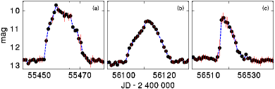
Figure 2: Examples of light curves of outbursts in RU Peg. (a) Bright outburst with a plateau on the top. (b) Outburst with a very long (slow) rising branch and a sharp peak. (c) Outburst with a very steep rising branch and a sharp peak. The standard deviations of brightness are marked. The points denote the 1-day means of brightness connected by the line to guide the eye. The distances between the ticks on each axis are the same for all plots. See Sect. 3 for details.

The crossing 12.2 mag in the rising, and the outburst’s decaying branches were used to measure its length $L$. The brightness varied rapidly in these outburst phases, which enabled us to determine these times with high accuracy (Fig. 1b).

The steepness of the rising branch of the outburst was measured between the brightnesses of 12.0 and 11.0 mag. The variety of the slopes was large here. The quantity $\tau_{\rm R}$ is expressed in days for an increase in brightness of 1 mag (Fig. 1c).

To investigate the asymmetry of the light curve of an outburst, we used the parameter $P$ defined in Eq. 1):

$$P=\frac{T_{\rm peak}-T_{\rm start}}{T_{\rm end}-T_{\rm start}}$$ (1)

where $T_{\rm peak}$ denotes the time of the peak of the outburst, $T_{\rm start}$ refers to the time of the start of this event (crossing its brightness 12.2 mag), and $T_{\rm end}$ refers to the time of its end (crossing its brightness 12.2 mag). These quantities were determined from the light curve of each well-covered event. Their uncertainties were used for the calculation of the standard deviation of $P$.

Equation 2) defines the outburst fluence $S$ (the observed optical energy output of the individual outbursts) as:

$$S=\int_{T_{\rm start}}^{T_{\rm end}}10^{0.4(12.2-V)}{\rm d}t$$ (2)

where $t$ is the time measured in days. Since we are interested in comparing the relative outputs of outbursts in a given DN, $S$ was expressed in dimensionless units (Fig. 1e).

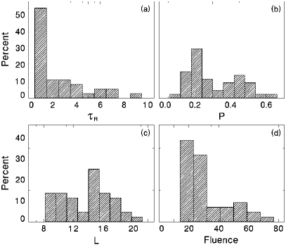
Figure 3: (a) Histogram of $\tau_{\rm R}$ of the outburst in RU Peg from Fig. 1c. (b) Histogram of parameter $P$ of the outburst from Fig. 1d. (c) Histogram of length $L$ of the outburst from Fig. 1b. (d) Histogram of fluences of the outbursts from Fig. 1e. See Sect. 3 for details.

In summary, out of the 52 detected outbursts, the reliable values of $L$, $P$, and fluence could be determined for 44 outbursts. The values of $\tau_{\rm R}$ could be determined for 37 outbursts. Figure 3 shows the histograms of some parameters of the outbursts of RU Peg. The histogram of $\tau_{\rm R}$ is very asymmetric, with a tail toward long $\tau_{\rm R}$ (Fig. 3a). The value of parameter $P$ of the outburst spans a broad range, with two mildly defined peaks of the vastly different heights (Fig. 3b). Figure 3c shows a flat histogram of $L$ with very mildly defined peaks. A very asymmetric histogram in Fig. 3d shows an extensive range of fluences of the outbursts.

A relation between the fluences and $L$ of the outbursts is displayed in Fig. 4a. Notice the very large scatter of $L$ for the fluences smaller than 30 (where most outbursts accumulate), followed by a long tail of the longer outbursts towards higher fluences. Since points are dispersed in both the direction of equal $L$ and equal fluences, variations of $L$ and outburst type contributed to the scatter.

Figure 4b shows that most outbursts occupy a small range of $\tau_{\rm R}<2$ d mag^-1, no matter how long these events are. Some outbursts with $L$ longer than 12 d (and especially $>14$ d) can have considerably bigger $\tau_{\rm R}$. In Fig. 4c, $\tau_{\rm R}$ is displayed vs $P$ taking into account the whole outburst. The relation of $\tau_{\rm R}$ and $P$ shows a group of outbursts with small $\tau_{\rm R}$, sharply turning into a gradual increase of $\tau_{\rm R}$ of outbursts with $P>0.3$.

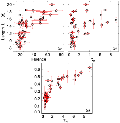
Figure 4: (a) Relation of fluences and $L$ of outbursts in RU Peg. Notice the large scatter of $L$ for the fluences smaller than 30, followed by a long tail toward bigger fluences. (b) Relation of $\tau_{\rm R}$ and $L$ of the outburst. (c) Relation of $\tau_{\rm R}$ and $P$ of the outburst. See Sect. 3 for details.

3.2 Profiles of the outbursts

The well-covered outbursts were plotted and superposed. We found that the best match was obtained when these outbursts were co-aligned according to their decaying branches. One outburst with a well-covered decaying branch was chosen as the template. The remaining outbursts were shifted along the time axis to match this template’s decaying branch (Fig. 5). The decay slopes remained mutually similar even if the peak position with respect to the outburst’s centre varied appreciably. Even a primarily variable $L$ of the outburst did not affect the slope of the decay.

The decaying branches of the individual outbursts were merged into a common file and smoothed by the code HEC13, written by Prof. P. Harmanec (Harmanec 1992). This code is based on the method of Vondrák (1969), who improved the original method of Whittaker (Whittaker & Robinson 1946). It can fit a smooth curve to the non-equidistant data no matter what their profile is. A full description can be found in Vondrák (1969). This method enables us to find a compromise between a curve running through all the observed points and an ideal smooth curve.

An ensemble of the best-covered outbursts was used for a fitting of the decaying branches. The input parameters of the fit $\epsilon=10^{-1}$, the length of the bin $\Delta$$T=0.05$ d satisfied the decaying branch of the ensemble. In our case, the input parameters were chosen so that the fit reproduced the decay’s main profile (Fig. 5).

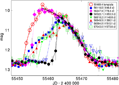
Figure 5: Light curves of the well-observed outbursts in RU Peg. The individual events were connected by the line to guide the eye. The error bars of the night means of brightness were marked. The individual events were shifted along the time axis to match the decaying branch of the template. The times of crossing 11.5 mag on the decay, $t_{\rm d}$, (in JD–2 400 000) and the shifts (in days) are listed. The thick dotted line represents a fit to an ensemble of the decaying branches of the outbursts. See Sect. 3 for details.

3.3 The outburst recurrence time and its variations

Because the outbursts of RU Peg are the discrete events with easily resolvable peaks, the method of the O–C residuals of some reference period is suitable for an analysis of their $T_{\rm C}$ (‘O’ stands for observed and ‘C’ for calculated times). Vogt (1980) applied this method to several DNe.

The resulting O–C curve also enabled us to assess each outburst’s position with respect to the O–C profile of the remaining outbursts. This method can work even if some outbursts are missing due to gaps in data, provided that the profile of the O–C curve is not too complicated.

Minimizing the slope of the O–C values generated for various $T_{\rm C}$ yielded $T_{\rm Cref}$, the reference value of $T_{\rm C}$. The resulting ephemeris is given in Eq. (3). Time of the basic peak of outburst, $T_{\rm b}$, is equal to JD 2 456 237, ${T_{\rm Cref}}$ is equal to 90 d, $E$ is epoch.

$$t_{\rm max}=T_{\rm b}+T_{\rm Cref}E$$ (3)

Figure 6a shows the complicated variations of the O–C curve around the mean value. Their amplitude is considerably larger than that of the rapid outburst-to-outburst fluctuations.

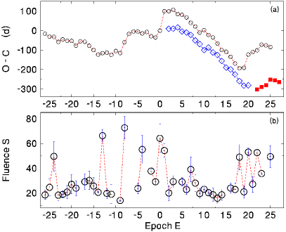
Figure 6: (a) The O–C diagram for the outbursts in RU Peg. The open circles represent the O–C values calculated according to Eq. 3 if we assume that we observed all outbursts. The errors of the O–C values are 1–4 d (comparable to the sizes of the symbols). The line connects the points considered to be the neighbouring outbursts. The open diamonds denote the O–C curve of nineteen outbursts with a missed outburst between epochs $E=0$ and $+1$. The filled squares denote a segment of the curve (six outbursts) with a missed outburst between $E=+19$ and $+20$. (b) The evolution of fluences of the outbursts in RU Peg with epoch $E$ from Eq. 3. A line connects the neighbouring outbursts for which their fluence could be determined reliably. See Sect. 3.3 for details.

Also, modifications of the O–C curve for several possible missed outbursts are shown in Fig. 6a. A long gap between the outbursts in the densely observed light curve in Fig. 7a shows that either no other outburst occurred between $E=-9$ and $E=-8$, or its peak magnitude was at least 2 mag lower than the surrounding events. Inclusion of the missed outbursts in seasonal gaps would alter the amplitude of the jumps in the O–C curve (especially, in Fig. 7b).

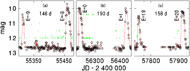
Figure 7: Light curves of surroundings of the potentially missed outbursts in RU Peg. Epochs of the two outbursts (Eq. 3) of each plot and their separation in days are listed. The points denote the 1-day means of brightness connected by the line to guide the eye. See Sect. 3 for details.

A comparison of the evolution of fluences with the O–C curve of $T_{\rm C}$ is shown in Fig. 6. The time segments of the relatively stable length of $T_{\rm C}$ (segments of $E$ between $-26$ and $-15$ and between $+2$ and $+17$) were accompanied by the mostly roughly stable and small values of fluence. On the contrary, the series of the enormous changes of $T_{\rm C}$ in other time segments were accompanied by the significant variations of outburst fluences.

4 Discussion

We present an analysis of the vigorous long-term optical activity of the DN RU Peg.

4.1 The outburst types

We ascribe outbursts of RU Peg shorter than about 12 d to be close to A-type (outside-in) outbursts because of their short $\tau_{\rm R}<2$ d mag^-1 (Fig. 4b). In the interpretation, while a bump in the histogram in Fig. 3c with shorter $L$ outbursts only contains the probable A-type events according to their $\tau_{\rm R}<2$ d mag^-1, the bump with $L$ longer than $12-14$ d consists of a mixture of outbursts of various types because of their largely variable $\tau_{\rm R}$ (up to about 9 d mag^-1). They may start at various distances from the disc centre, $r_{\rm s}$, and span between the A and B-types (inside-out). These outburst types were defined in the model of Smak (1984).

Bimodal histograms of $L$ of DNe are usual, and the prominence of the peaks differs from system to system (Ak et al. 2002). Although this separation is somewhat blurred in RU Peg, it also reflects the contribution of the different outburst types in RU Peg (Fig. 3c).

Furthermore, outbursts of RU Peg occur in the restricted $\tau_{\rm R}$ vs $P$ region (Fig. 4c). While $\tau_{\rm R}$ represents the steepness of the rising branch, $P$ refers to the asymmetry of the outburst (given primarily by the whole rising branch and plateau because the decaying branches are mutually similar (Fig. 5)). For example, no outbursts which may be close to the $B$-type contain a significant plateau because we detect no outbursts in the region of $\tau_{\rm R}>3$ and $P<0.3$. In this context, the first bump in the histogram in Fig. 3b represents outbursts similar to the A-type, the second bump in Fig. 3b represents the tail which starts at $P\approx 0.35$ in Fig. 4c and may contain a mixture of various outburst types. It confirms the result in Fig. 3c.

The rising branches in Fig. 5 show a transition from the big initial steepness to the subsequent less steep rise in the different phases since the start for the individual outbursts (e.g., outbursts with $t_{\rm d}=2\,456\,118$ and $t_{\rm d}=2\,456\,618$, both ascribed to be similar to the B-type). We interpret it as the outburst starts at the different values of $r_{\rm s}$ in RU Peg. A discrepancy between outburst types and fluences can be explained by the dispersion of data for the fluences smaller than 30 in both the direction of equal $L$ and equal fluences in Fig. 4a. It shows that both variations of $L$ and outburst type contributed to the scatter. A detailed analysis of the rise of outbursts (e.g., orbital modulation) and a comparison with models will be helpful.

As regards the differences between the outburst types in RU Peg, the probable A-type outburst with $t_{\rm d}=2\,456\,522.7$, $\tau_{\rm R}=0.6$ d mag^-1 was considerably shorter than the probable B-type event with $t_{\rm d}=2\,456\,118.0$, $\tau_{\rm R}=6.9$ d mag^-1) (Fig. 5). In the Smak (1984) model framework, we interpret this short likely A-type outburst as starting by reaching the critical column density in a narrow ring at the outer disc rim. It is also possible to assess the values of $r_{\rm s}$ of the future events by comparing models of relative delays between the optical and ultraviolet outburst light curves because outbursts close to the A-type have the UV delay considerably more prominent than the B-types (Smak 1998). Also, the changes in Doppler tomograms can shed more light; such a tomogram exists only for one outburst (Dunford et al. 2012). Although the investigation of the evolution of the orbital modulation during the start of various outbursts of RU Peg might pinpoint the location of the trigger of the instability, $i\approx 33^{\circ}$ (Friend et al. 1990) indicates its low amplitude and the absence of eclipses.

4.2 Disc overflow

Although the B-type is typical for DNe with $\dot{m}_{\rm tr}$ lower than the A-type (Smak 1984), we interpret the large variety of the light curves as the starts of outbursts of RU Peg at various values of $r_{\rm s}$, even in roughly the same $T_{\rm C}$ (Figs. 1 and 6a). Disc overflow may occur for some outbursts to modify $r_{\rm s}$ of the ring of the disc matter reaching the critical column density. It gives rise to the accumulation of matter in the different $r_{\rm s}$ even at a roughly constant value of $\dot{m}_{\rm tr}$ in the model of Schreiber & Hessman (1998).

This disc overflow, varying with time, could also contribute to the change of $\tau_{\rm R}$ and $P$. Doppler tomography of RU Peg in one outburst (Dunford et al. 2012) shows a highly asymmetric extension of the width of the mass stream. Such tomograms obtained in various outbursts and quiescences could help assess how and at which places the collision of the inflowing matter and the disc occurs at various times. Also, theoretical studies of the effect of this merging on the outburst types and $T_{\rm C}$ are desirable.

4.3 Disc irradiation

We found that the properties of the decaying branches of the outbursts (hence the properties of the cooling front determining the decay rate of these outbursts (e.g., Smak 1984; Hameury et al. 1998)) of RU Peg were stable and reproducible for the individual events, no matter how steep the rising branches (whether close to the A or B-type) and how long the outbursts were (Fig. 5). The profiles of the outbursts’ decays in RU Peg place the constraints on the strength of irradiation of the disc from the very hot WD (50 000–70 000 K (Sion & Urban 2002; Godon et al. 2008)) and the donor, as modelled by Hameury et al. (1999, 2000). The Hameury et al. (2000) model predicts several noticeable rebrightenings on the decaying branch of the outburst if the hot WD strongly irradiates the disc. However, these branches are smooth in RU Peg, with well-reproducing profiles. This speaks in favour of no significant irradiation of the disc by the WD. It could be reconciled by evaporation of the inner disc region in an outburst of RU Peg, modelled by Hameury et al. (1999). However, this evaporation would have to be strong enough no matter how big the fluence of the outburst was.

In this regard, the mutual similarity of the smooth decaying branches of the individual events in a given DN, irrespective of the rising branches and the length of $P_{\rm orb}$, is more general (e.g., SS Cyg (Cannizzo & Mattei 1998), DX And (Šimon 2000b), X Ser (Šimon 2018a)). This ensemble also includes DO Dra (Šimon 2000a) and GK Per (Šimon 2002), which are intermediate polars (IPs) (Haswell et al. 1997; Patterson et al. 1992; Watson et al. 1985; Crampton et al. 1986). IPs accrete onto the WD’s polar caps in an outburst, not onto the boundary layer (Warner & McGraw 1981; Warner 1995). All of this speaks in favour of only weak irradiation of their discs, whether they accrete via boundary layer or polar caps. Because the propagation of a cooling front is not affected by irradiation at large values of $r_{\rm s}$, we do not expect any difference between magnetised and non-magnetised WD. Also, a low $T_{\rm eff}$ of the WD, evaporation of the inner disc region or a complicated structure of the inner disc region can contribute to preventing the disc from intense irradiation by the WD.

A flattening of the decay rate of most outbursts of RU Peg in their final phases, about 0.4 mag above quiescence, can be explained by an increase of the mass outflow from the donor’s nozzle due to its irradiation in the advanced phase of the outburst (see the model of Hameury et al. 2000). Indeed, this irradiation in outburst was detected on the Roche tomograms of Dunford et al. (2012). Also, the light contribution of the secondary component, the WD and the hot spot are likely to contribute to this outburst phase. This behaviour is different from that in SS Cyg (Cannizzo & Mattei 1998), in which the decay rate of some outbursts displays a glitch about 0.8–1 mag above quiescence, and then continues with the same decay rate as before. Investigation of the evolution of the orbital modulation and the roles of the light contributions of various system components of such DNe in these phases will be helpful.

4.4 The variations of $T_{\rm C}$

The variations of $T_{\rm C}$ between the neighbouring (or nearby) outbursts were much smaller than the length of $T_{\rm C}$ in RU Peg. Several episodes of the abrupt changes (jumps) were detected (Fig. 6a). All of this speaks in favour of mutually dependent outbursts, although the fluence was not related to the current length of $T_{\rm C}$. In the TVI model (Smak 1984; Hameury et al. 1998), only a small part of the disc matter is accreted from the disc in outbursts. Whether the outburst of RU Peg was closer to the A-type or the B-type and how big $L$ and fluence were (Figs. 1 and 6), it did not deviate from the O–C curve of other outbursts. The processes in the cool disc thus played a significant role. This curve of RU Peg is similar to those in other DNe of various subtypes (e.g., Vogt 1980; Šimon 2000b; Šimon 2002).

A combination of the fluences with the evolution of $T_{\rm C}$ showed several time segments with the different behaviours of RU Peg. The time segments with little variable fluences, accompanied by a relatively stable length of $T_{\rm C}$, were sometimes replaced by the time segments with a more remarkably variable $T_{\rm C}$ and scatter of fluences. The change reaching the peak-to-peak amplitude of the scatter of fluences was sometimes achieved rapidly, even during the neighbouring outbursts (Fig. 6). A bigger fluence suggests more matter accreted from the disc onto the WD during this outburst (e.g., Smak 1984; Hameury et al. 1998) irrespective of whether it was closer to the A or B-type.

The extremely large fluences of some outbursts, occurring only in the events with excessively long $L$ ($>14$ d) (Fig. 4a) between $E=-14$ and $E=+2$ bear the similarity to a very long outburst of U Gem (Cannizzo et al. 2002), attributed to an increase in the mass transfer rate from the donor to the disc during the DN outburst. In the interpretation, the activity of the donor in RU Peg (e.g., an increase of the mass outflow through the L₁ point) caused considerable variations of fluence. We attribute it to destabilising the disc and $T_{\rm C}$ without any definite correlation in this time segment.

Also, a prominent jump near $E=+18$ is an example that the relation between $\dot{m}_{\rm tr}$ and $T_{\rm C}$ of RU Peg can be exceeded by other processes. A model with a variable outer disc boundary (Hameury et al. 1998) shows that an increase of $\dot{m}_{\rm tr}$ by a factor of ten leads to a shortening of $T_{\rm C}$ by about 50% and broader, more luminous outbursts. Although the jump near $E=+18$ gives an increase of $T_{\rm C}$, a series of the large variations of the outburst fluences (with a significant fraction of outbursts with large fluences, hence increases of the amount of the accreted matter) started in the vicinity of this jump (Fig. 6). We ascribe the decrease of $\tau_{\rm R}$ and $P$ since the vicinity of $E=+18$ to the dominance of the A-type events, accompanying this change of $T_{\rm C}$ (Figs. 1c and 1d). We ascribe this episode to a change of the disc structure.

Rapid variations of $T_{\rm C}$ can also be caused by a variable removal of angular momentum from the matter in the disc, for example, if the magnetic field from the starspots on the secondary reaches over to the disc (Meyer-Hofmeister et al. 1996). In this model, the interaction of this field with the disc leads to shorter DN outbursts and a decrease of $T_{\rm C}$ for a given mass transfer rate between the components. The time segments in which the effect of this field on the disc dominates (e.g., no bursts of matter from the donor occur) might explain the relatively stable and short $T_{\rm C}$, accompanied by the small fluences and the often small $L$ in $E$ between $-23$ and $-15$ and especially between $+2$ and $+17$ in RU Peg (Fig. 6a).

In conclusion, a combination of the variations of $T_{\rm C}$ with the complicated and unstable properties of the outbursts, including an unstable mass transfer rate between the components, suggest the dominance of several mechanisms on the state of the disc of RU Peg in various time segments.

Data availability

The dataset was derived from a source in the public domain.

References

- [1] Ak T., Ozkan M. T., & Mattei J. A., 2002, A&A, 389, 478
- [2] Bailer-Jones C. A. L., Rybizki J., Fouesneau M., Mantelet G., & Andrae R., 2018, AJ, 156, 58
- [3] Balman Şölen, Godon Patrick, Sion Edward M., Ness Jan-Uwe, Schlegel Eric, Barrett Paul E., & Szkody Paula, 2011, ApJ, 741, 84
- [4] Cannizzo John K., & Mattei Janet A., 1998, ApJ, 505, 344
- [5] Cannizzo John K., Gehrels Neil, & Mattei Janet A., 2002, ApJ, 579, 760
- [6] Crampton D., Cowley A. P., & Fisher W. A., 1986, ApJ, 300, 788
- [7] Dobrotka A., Mineshige S., & Ness J.-U., 2014, MNRAS, 438, 1714
- [8] Dubus Guillaume, Otulakowska-Hypka Magdalena, & Lasota Jean-Pierre, 2018, A&A, 617, A26
- [9] Dunford A., Watson C. A., & Smith Robert Connon, 2012, MNRAS, 422, 3444
- [10] Friend M. T., Martin J. S., Smith R. C., & Jones D. H. P., 1990, MNRAS, 246, 654
- [11] Gaia Collaboration: Brown A. G. A. et al. 2018, A&A, 616, A1
- [12] Godon Patrick, Sion Edward M., Barrett Paul E., Hubeny Ivan, Linnell Albert P., & Szkody Paula, 2008, ApJ, 679, 1447
- [13] Hameury Jean-Marie, Menou Kristen, Dubus Guillaume, Lasota Jean-Pierre, & Hure Jean-Marc, 1998, MNRAS, 298, 1048
- [14] Hameury Jean-Marie, Lasota Jean-Pierre, & Dubus Guillaume, 1999, MNRAS, 303, 39
- [15] Hameury J.-M., Lasota J.-P., & Warner B., 2000, A&A, 353, 244
- [16] Hameury J. M., 2020, AdSpR, 66, 1004
- [17] Harmanec P., 1992, the Fortran source version, compiled version, brief instructions: http://astro.troja.mff.cuni.cz/ftp/hec/HEC13/
- [18] Haswell C. A., Patterson J., Thorstensen J. R., Hellier C., & Skillman D. R., 1997, ApJ, 476, 847
- [19] Howarth I. D., 1975, JBAA, 85, 271
- [20] Kafka S., 2019, Observations from the AAVSO International Database, http://www.aavso.org
- [21] Meyer-Hofmeister E., Vogt N., & Meyer F., 1996, A&A, 310, 519
- [22] Patterson J., 1984, ApJS, 54, 443
- [23] Patterson J., Schwartz D. A., Pye J. P., Blair W. P., Williams G. A., & Caillault J.-P., 1992, ApJ, 392, 233
- [24] Pearson K. J., Wynn G. A., & King A. R., 1997, MNRAS, 288, 421
- [25] Percy J. R., Fabro V. A., & Keith D. W., 1985, J. AAVSO, 14, 1
- [26] Richman H. R., Applegate J. H., & Patterson J., 1994, PASP, 106, 1075
- [27] Ritter H., & Kolb U., 2003, A&A, 404, 301
- [28] Samus N. N., Kazarovets E. V., Durlevich O. V., Kireeva N. N., & Pastukhova E. N., General Catalogue of Variable Stars: Version GCVS 5.1, Astronomy Reports, 2017, vol. 61, No. 1, pp. 80-88
- [29] Schreiber M. R., & Hessman F. V., 1998, MNRAS, 301, 626
- [30] Šimon V., 2000a, A&A, 360, 627
- [31] Šimon V., 2000b, A&A, 364, 694
- [32] Šimon V., 2002, A&A, 382, 910
- [33] Šimon V., 2018a, A&A, 614, A141
- [34] Šimon V., 2018b, Proceedings of Science, Volume 331, Article number 58, 3rd Frontier Research in Astrophysics, FRAPWS 2018
- [35] Šimon V., 2019, https://www.plate-archive.org/applause/project/lswst/lswst1/
- [36] Sion Edward M., & Urban Joel, 2002, ApJ, 572, 456
- [37] Smak J., 1984, Acta Astron., 34, 161
- [38] Smak, Jozef I., 1998, AcA, 48, 677
- [39] Stover R. J., 1981, ApJ, 249, 673
- [40] Vogt N., 1980, A&A, 88, 66
- [41] Vondrák J., 1969, Bull. Astron. Inst. Czechosl., Vol. 20, 349
- [42] Warner B., & McGraw J. T., 1981, MNRAS, 196, 59
- [43] Warner B., 1995, Cataclysmic Variable Stars, Cambridge Univ. Press, Cambridge
- [44] Warner Brian, 1998, ASPC, 137, 2
- [45] Watson M. G., King A. R., & Osborne J., 1985, MNRAS, 212, 917
- [46] Whittaker E., & Robinson G., 1946, The Calculus of Observations, Blackie & Son Ltd, London, pp. 303-316