Decision-Focused Learning: Through the Lens of Learning to Rank

Abstract

In the last years, decision-focused learning, also known as predict-and-optimize, has received increasing attention. In this setting, the predictions of a machine learning model are used as estimated cost coefficients in the objective function of a discrete combinatorial optimization problem for decision making. Decision-focused learning proposes to train the ML models, often neural network models, by directly optimizing the quality of decisions made by the optimization solvers. Based on a recent work that proposed a noise contrastive estimation loss over a subset of the solution space, we observe that decision-focused learning can more generally be seen as a learning-to-rank problem, where the goal is to learn an objective function that ranks the feasible points correctly. This observation is independent of the optimization method used and of the form of the objective function. We develop pointwise, pairwise and listwise ranking loss functions, which can be differentiated in closed form given a subset of solutions. We empirically investigate the quality of our generic methods compared to existing decision-focused learning approaches with competitive results. Furthermore, controlling the subset of solutions allows controlling the runtime considerably, with limited effect on regret.

1 Introduction

Many real-world decision making problems rely on the combination of machine learning (ML) and combinatorial optimization (CO). In those applications, CO problems are solved to arrive at a decision by maximizing or minimizing an objective function. However, often some parameters of the optimization problem, such as costs, prices and profits, are not known but can be estimated from other feature attributes based on historical data.

A two-stage predict-then-optimize approach is widely used by practitioners in both the industry and the public sector, where first an ML model is trained to make point estimates of the uncertain parameters and then the optimization problem is solved using the predictions. However, this treats the parameter errors as independent and does not take the interplay of the parameter errors and their effect on the combinatorial optimisation problem into account.

Recently decision-focused learning (Wilder et al., 2019; Pogancic et al., 2020) (also known as predict-and-optimize (Elmachtoub & Grigas, 2021; Mandi et al., 2020)) has received increasing attention. In this setting, during training, the ML model is trained with a loss function that first solves the downstream CO problem to observe the joint error. On the technical level, the challenge of integrating combinatorial optimization into the training loop of ML is the non-differentiability of combinatorial problems. To address this, Mulamba et al. (2021) recently proposed an approach motivated by noise-contrastive estimation (Gutmann & Hyvärinen, 2010), where they introduce a new family of surrogate loss functions considering non-optimal feasible solutions as negative examples. In their work, they propose a surrogate loss function, which maximizes the divergence between the objective values of the true optimal and the negative examples.

We argue that decision-focused learning can be more generally viewed through the lens of learning to rank (LTR) approach (Burges et al., 2005). In a LTR problem, for each query there is a list of items and their feature variables given. The training objective is to learn a ranking function, which will rank the (top) items correctly for each query.

In the context of CO problems, a partial ordering of the feasible solutions is induced by the objective function. Learning the orders of the feasible solution with respect to the objective function hence achieves the goal of decision-focused learning. When compared to the LTR literature, there are two important differences: 1) part of the structure of the objective function is already given, only some of its parameters must be estimated; and 2) the set of ‘items’ are all feasible solutions, which are the same for all CO problem instances (queries), but it is intractable to enumerate all. While backpropagating, 1) needs not be an issue under the assumption that just the objective function itself is differentiable, which is the case for standard continuous functions including linear functions. With respect to 2), we can subsample the feasible solutions as is done by Mulamba et al. (2021).

The main contributions of this work are the following: First, we formulate the decision-focused learning  as a ranking problem. Secondly, we introduce and study several well-known learning to rank loss functions. In particular, we formulate pointwise, pairwise and listwise ranking loss functions for decision-focused learning problems. Thirdly, we show that the pairwise ranking loss is a generalization of the loss functions proposed by Mulamba et al. (2021). Lastly, we show that in case of a linear objective function, the pointwise and pairwise-difference loss functions can be interpreted as trading off the mean square error (MSE) and regret of predictions.

2 Related Literature

Decision-focused learning.

Decision-focused learning involves optimization problems, where the optimization parameters are defined partially. One of the major developments in this topic is the differentiable optimization layer (Amos & Kolter, 2017), which analytically computes the gradients by differentiating the KKT optimality conditions of a quadratic program. The gradient calculation of Amos & Kolter (2017) does not translate to linear programming (LP) problems due to singularities of the objective function in this case. Wilder et al. (2019) address this by introducing a small quadratic regularizer in the objective function while Mandi & Guns (2020) introduce a log-barrier regularization term and compute the gradients from the homogeneous self dual embedding of the LP. Ferber et al. (2020) studies mixed integer LPs and reduce it to LP by adding cutting plane to the root LP node, applying the framework of Wilder et al. (2019) afterwards. All these methods are specific to the structure of the CO problem used.

Other approaches are independent of the CO problem and solver used. The smart predict-and-optimize approach of Elmachtoub & Grigas (2021) studies optimization problems with linear objectives and where the cost vector has to be predicted. They introduce a convex surrogate upper bound of the loss and propose an easy to use subgradient. Pogancic et al. (2020) also studies problems with linear objectives. They compute the gradient by perturbing the predicted cost vector. Niepert et al. (2021) extend this work by adding noise-perturbations for perturbation-based implicit differentiation. For an overview of decision-focused learning, we refer the readers to Kotary et al. (2021).

All these approaches involve solving the optimization problem for every instance during training, which comes at a very high computational cost. To address this problem, Mulamba et al. (2021) propose contrastive loss functions with respect to a pool of feasible solutions of the optimization problem. It cleanly separates the solving (adding solutions to the pool), from the loss function. This allows the loss function to be differentiated directly. We build on this idea but through the lens of learning to rank.

Learning to rank.

Learning to rank problems have been studied thoroughly over the years, especially within the context of information retrieval. Readers can refer to Liu (2011) for a detailed analysis. Most of the LTR approaches assign real-valued scores to the items, then define surrogate loss functions on the scores. In pointwise LTR models (Li et al., 2007), the labels are the rank (or true score, if known) of the items. These models fail to consider any inter dependencies across the item rankings. Pairwise ranking approaches (Burges et al., 2005) aim to learn the relative ordering of pairs of items. Finally, listwise approaches (Cao et al., 2007) define loss functions with respect to the scores of the whole ranked lists. The LTR framework has been applied to various contexts such as recommender systems (Karatzoglou et al., 2013) and software debugging (Xuan & Monperrus, 2014), among others.

Demirović et al. (2019) have used LTR in decision-focused learning framework, but by considering the parameters of a linear objective function as the items to rank, e.g. the value of items of a knapsack problem, instead of the feasible solutions as we do. Kotary et al. (2021) propose a fair LTR methodology, which impose fairness constraints using constraints in the combinatorial optimization problem and they use decision-focused learning to integrate the optimization program with an ML model. In contrast, we use LTR models and losses for decision-focused learning.

3 Problem Statement and Motivation

In this section, we introduce the decision-focused learning setup. We consider a discrete combinatorial optimization problem

$$v^{\star}(c)\in\operatorname*{argmin}_{v\in V}f(v,c)$$ (1)

where $V\subseteq\mathbb{Z}^{K}$ is the set of feasible integer solutions, typically specified implicitly through constraints, and $f:V\times\mathcal{C}\rightarrow\mathbb{R}$ is the real valued objective function, where $\mathcal{C}\subset\mathbb{R}^{K}$ is the domain of the vector of parameters $c$. We denote an optimal solution of (1) by $v^{\star}(c)$. The value of $c$ is unknown but we have access to correlated features $x$ and a historic dataset $D=\{(x_{i},c_{i})\}_{i=1}^{N}$. The goal is to predict the apriori unknown coefficient vector $c_{i}$ in a supervised machine learning setup. To do so, we train a model noted by $m(\omega,x_{i})$ to make a prediction of vector $c_{i}$, where $\omega$ are the model parameters. Let us denote the predicted value as $\hat{c}_{i}=m(\omega,x_{i})$.

In a traditional supervised machine learning setup, we train by minimizing the difference between $c$ and $\hat{c}$. For instance, in a regression problem, we minimize the multi-output mean square error,

$$\mathbf{mse}(c,\hat{c})=\sum_{k=1}^{K}(c_{k}-\hat{c}_{k})^{2}=\sum_{k=1}^{K}\epsilon_{k}^{2}$$ (2)

where $\epsilon_{k}=(c_{k}-\hat{c}_{k})$, over a set of $N$ instances $\{(c,\hat{c})\}$.

In contrast, in decision-focused learning $\hat{c}$ is an intermediate result. The final output is $v^{\star}(\hat{c})$, the solution of the discrete combinatorial optimization problem. The final goal is to minimize the impact of the solution $v^{\star}(\hat{c})$ in the downstream optimization problem whenever the real cost vector $c$ is realized. In order to measure how good $\hat{c}$ is, we compute the regret of the combinatorial optimisation. The regret is defined as the difference between the value of the optimal objective value $f(v^{\star}(c),c)$ and the value of the objective function with ground truth $c$ and predicted solution $v^{\star}(\hat{c})$. Formally, we define regret, without any assumptions on the structure of $f$, as

$$\mbox{Regret}(\hat{c},c)=f(v^{\star}(\hat{c}),c)-f(v^{\star}(c),c).$$ (3)

Ideally, we aim to learn parameters $\omega$ that determine $\hat{c}=m(\omega,x)$ such that it minimizes the regret. To do so in a neural network setup, the gradient of the regret has to be backpropagated, which requires computing the exact derivative of the regret (3). This task is problematic as $V$ is discrete and the regret function is non-continuous and involves differentiating over the argmin in $v^{\star}(\hat{c})$.

As mentioned in section 2, several recent works have studied this problem. However, in all those cases, in order to compute the gradient, the optimization problem (1) must be solved repeatedly for each instance during training. Hence, scalability is a major challenge in these approaches.

3.1 Contrastive Surrogate Loss

To improve the scalability of decision-focused learning Mulamba et al. (2021) proposed an alternative class of loss functions. They first define the following probability distribution of $v\in V$ being the optimal one.

$$p(v|c)=\begin{cases}\frac{\exp\left(-f\left(v,c\right)\right)}{\sum_{v^{\prime}\in V}\exp\left(-f\left(v^{\prime},c\right)\right)}&\text{if}\ v\in V\\ 0,&\text{if}\ v\notin V\end{cases}$$ (4)

It is easy to verify that, if $v$ is one minimizer of Eq. 1, then it will maximize Eq. 4. To define the loss functions they consider to have access to $S$, a subset of $V$ and treat $\left(S\setminus\{v^{\star}(c)\}\right)$ as negative examples. With this setup, they define the following noise contrastive estimation (NCE) loss

$$L_{\operatorname*{NCE}}(\hat{c},c)=\frac{1}{|S|}\sum_{v^{s}\in S}\Big{(}f\big{(}v^{\star}(c),\hat{c}\big{)}-f\big{(}v^{s},\hat{c}\big{)}\Big{)}.$$ (5)

The novelty of this approach is that Eq. (5) is differentiable and that the differentiation does not involve solving the optimization problem in (1). Further, if the solutions in $S$ are optimal solutions of arbitrary cost vectors, this approach is equivalent to training in a region of the convex-hull of $V$.

4 Rank Based Loss Functions

In this section we develop and motivate a family of surrogate loss functions for decision-focused learning problems. We remark that, for a given $c$, we can create a partial ordering of all $v\in V$ by ordering them with respect to the objective value. Let us denote by $p_{1},\ldots,p_{|V|}$ the indices of $V$ so that $f(v^{p_{1}},c)\leq f(v^{p_{2}},c)\leq\ldots\leq f(v^{p_{|V|}},c)$. The key idea of our approach is to generate prediction $\hat{c}$ so that $f(v^{p_{1}},\hat{c})\leq f(v^{p_{2}},\hat{c})\leq\ldots\leq f(v^{p_{|V|}},\hat{c})$. Notice that, if the ranks of $v\in V$ with respect to $\hat{c}$ are identical to that of $c$, the regret is zero. Furthermore, it is sufficient that $\forall p_{s}:f(v^{p_{1}},\hat{c})\leq f(v^{p_{s}},\hat{c})$ for the regret to be zero. In general, our surrogate task is to learn the ranking of each $v\in V$ with respect to $c$. This motivates us to use the LTR framework to develop a new class of surrogate loss functions for decision-focused learning problems.

Drawing a parallel to the LTR literature, we consider each $x$ a query, and the feasible solutions $v\in V$ as the set of items to be ordered. Our formulation differs from traditional LTR framework because in LTR problems each item has its own set of feature variables, whereas in our formulation each $v$ does not have feature variables. We hence only have query-features ($x$ itself) to predict $c$. In the LTR framework, a ranking function is used to assign scores to each item. In decision-focused learningsetup, we will consider the objective function $f(v,c)$ as the scoringh function.

To rank all $v\in V$ is an intractable task for most combinatorial problems. To overcome this in practice, we will consider a set of feasible solution $S\subset V$. The proposed implementation is described in pseudocode form in Algorithm 1. For each $c$, we compute a loss function $L(\hat{c},c)$ considering the surrogate ranking task. The implementation details are described later. Next, we will introduce the family of rank based loss functions.

Algorithm 1 Gradient-descent implementation of decision-focused learning problems with Ranking Loss

Input: D$\equiv\{(x_{i},c_{i})\}_{i=1}^{n}$

1:  Initialize $\omega$

2:  Initialize $S=\{v^{\star}(c_{i})|(x_{i},c_{i})\in D\}$ Training

3:  for each epochs do

4:     for each $(x_{i},c_{i})$ do

5:        $\hat{c}_{i}=m(\omega,x_{i})$

6:        if random$()<p_{solve}$ then

7:           $v^{\star}(\hat{c}_{i})\leftarrow$call solver to solve Eq. (1),

8:           $S\leftarrow S\cup\{v^{\star}(\hat{c}_{i})\}$

9:        end if

10:        $\mathcal{L}+=L(\hat{c}_{i},c_{i};S)$

11:     end for

12:     $\omega\leftarrow\omega-\alpha\frac{\partial\mathcal{L}}{\partial\omega}$ # backward pass

13:  end for

4.1 Pointwise Ranking

In pointwise ranking loss formulation, the loss function is defined for each item (feasible solution) independently. In our pointwise rank loss formulation, we propose to regress the predicted objective function value on the actual objective function value. Thus, we propose the pointwise loss function

$$L_{P}(\hat{c},c;S)=\frac{1}{|S|}\sum_{v\in S}\left(f(v,\hat{c})-f(v,c)\right)^{2}$$ (6)

that measures the errors in the evaluation of the predicted cost function at each point in $S$.

Intuitive idea of the pointwise loss function.

When the objective function is linear i.e. $f(v,c)=c^{\intercal}v$, the pointwise loss (6) becomes

$$L^{p}(\hat{c},c;S)=\frac{1}{|S|}\sum_{v\in S}\left(c^{\intercal}v-\hat{c}^{\intercal}v\right)^{2}$$ (7)

The derivative of this loss is

$$\frac{\partial L^{p}(\hat{c},c;S)}{\partial\hat{c}}=-\frac{2}{|S|}\sum_{v\in S}\left(c^{\intercal}v-\hat{c}^{\intercal}v\right)v$$ (8)

When considering a combinatorial problem where $v$ is a binary vector, we can see from Eq. (8) that coordinates where $v$ has zeros, will not contribute to the gradient. Moreover, the first component $\left(c^{\intercal}v-\hat{c}^{\intercal}v\right)$ is the difference between the actual and the predicted objective value on $v$. The gradient contribution of $v$ is weighed by this difference.

Pointwise loss as a regularizer.

For the special case of a linear objective function $f(v,c)=$ $\sum_{j=1}^{K}c_{j}v_{j}$, the pointwise task loss can be rewritten as:

$$L_{P}(\hat{c},c;S)= \sum_{i=1}^{K}(\hat{c}_{i}-c_{i})^{2}\gamma_{i}+\sum_{i\neq j}(\hat{c}_{i}-c_{i})(\hat{c}_{j}-c_{j})\gamma_{ij}$$

$$= \sum_{i=1}^{K}\epsilon_{i}^{2}\gamma_{i}+\sum_{i\neq j}\epsilon_{i}\epsilon_{j}\gamma_{ij}$$ (9)

where $\gamma_{i}=\frac{1}{|S|}\sum_{v\in S}v_{i}^{2}$ and $\gamma_{ij}=\frac{1}{|S|}\sum_{v\in S}v_{i}v_{j}$ and $\epsilon_{i}$ defined as in (2). In this case, it is a weighted version of the $\mathbf{mse}$ function plus a term that measures the pairwise relationship of errors of the coordinates.

Moreover, when $V\subseteq\{0,1\}^{K}$, the weight $\gamma_{i}$ is the frequency of how many times coordinate $v_{i}$ takes value 1 (since $v_{i}^{2}=v_{i}$). Coefficients $\gamma_{ij}$ measure the frequency where $v_{i}$ and $v_{j}$ take value 1 at the same time. In particular, if $S=V$

$$L^{p}(\hat{c},c;V)=\frac{1}{2}\Big{(}\mathbf{mse}(\hat{c},c)+\sum_{i=1}^{K}\sum_{j=1:j<i}^{K}\epsilon_{i}\epsilon_{j}\Big{)}$$

Hence, the pointwise loss function can be seen as the $\mathbf{mse}$ plus a regularizer which penalizes the crossed-errors between coordinates of the vector $c$.

4.2 Pairwise Ranking

Example. To demonstrate the shortcoming of the pointwise loss and the motivation behind the pairwise loss formulation, we construct a simple example. Let us consider the feasible space is the 2 dimensional 0-1 space, containing the four feasible points $[0,0],[0,1],[1,0],[1,1]$. Now, let $c$ be $[2,-5]$. The objective values at these four points are $0,-5,2$ and $-3$, hence $v^{\star}(c)=[0,1]$. Now let $\hat{c}_{1}$ be $[-1,1]$ and $\hat{c}_{2}$ be $[5,-11]$. For $\hat{c}_{1}$ and $\hat{c}_{2}$, the objective values of these four points are $0,1,-1,0$ and $0,-11,5,-6$ respectively. The square error of both $\hat{c}_{1}$ and $\hat{c}_{2}$ is $45=(3^{2}+6^{2})$. The pointwise loss between $c$ and $\hat{c}_{1}$ is $54=(0+(-5-1)^{2}+(2+1)^{2}+(-3-0)^{2})$ and $c$ and $\hat{c}_{2}$ is $54=(0+(-5+11)^{2}+(2-5)^{2}+(-3+6)^{2})$. But $v^{\star}(\hat{c}_{1})=[1,0]$ and $v^{\star}(\hat{c}_{2})=[0,1]=v^{\star}(c)$. Even though the regret of $\hat{c}_{2}$ is $0$, its pointwise loss is the same as $\hat{c}_{1}$, whose regret is positive. With this motivation behind, we will construct the pairwise ranking loss function.

Let $(p,q)$ be an ordered pair in $S$ with respect to $c$. We define $\mbox{OP}_{c}^{S}$ as the set of all the ordered pairs such that the first coordinate dominates the second one in the order induced by $c$, or equivalently:

$$(p,q)\in\mbox{OP}_{c}^{S}\implies f(v^{p},c)<f(v^{q},c)$$ (10)

For an ordered pair $(p,q)$, we expect the predicted $\hat{c}$ would also respect the ordering i.e. $f(v^{p},\hat{c})<f(v^{q},\hat{c})$. In other words, $f(v^{p},\hat{c})-f(v^{q},\hat{c})$ is the quantity we aim to minimize. In the standard pairwise margin ranking loss formulation (Joachims, 2002), the loss is zero, if $f(v^{p},\hat{c})$ is smaller than $f(v^{q},\hat{c})$ by at least a margin of $\nu>0$. With this notion of margin, we introduce the following generic pairwise loss

$$\operatorname*{L_{\mbox{OP}^{S}_{c}}}(\hat{c},c)=$$

$$\frac{1}{|\mbox{OP}_{c}^{S}|}\sum_{(p,q)\in\mbox{O.P.}_{c}^{S}}\max\left(0,\nu+f(v^{p},\hat{c})-f(v^{q},\hat{c})\right)$$ (11)

Ordered pairs generation.

Eq. (11) is built upon the concept of a pairwise ranking loss (Burges et al., 2005). Note that, to implement this approach we have to identify ordered pairs from the negative examples. Clearly generating all possible pairs comes with a complexity of $\mathcal{O}(|S|^{2})$. To overcome this implementation challenge, we consider best-versus-rest scheme, i.e. $\mbox{OP}_{c}^{S}=\{(v^{p_{1}},v^{p_{2}}),(v^{p_{1}},v^{p3}),\ldots,(v^{p_{1}},v^{p_{S}})\}$, where $v^{p_{1}}=v^{\star}(c)$. With this best-versus-rest pair generation scheme and $\gamma$ being $0$, Eq. (11) becomes

$$\frac{1}{|S|}\sum_{v^{q}\in S}\max\left(0,(f(v^{\star}(c),\hat{c})-f(v^{q},\hat{c}))\right)$$ (12)

We point out that (12) takes the form of (5), without the relu operator. This shows that the NCE approach of Mulamba et al. (2021), although derived differently, can be seen as a special case of our best-versus-rest pairwise approach.

Example continued. For computing the pairwise loss, first, we have to generate the ordered pairs. The ordering of the feasible points with respect to $c$ is $[0,1],[1,1],[0,0],[1,0]$. Following the best-vs-rest scheme, the pairs are $\{([0,1],[1,1]),([0,1],[0,0]),([0,1],[1,0])\}$. For $\hat{c}_{1}$ the value of the pairwise loss is $1+1+2=4$. For $\hat{c}_{2}$ the value of pairwise loss is $0+0+0=0$, which is reasonable as its regret is $0$.

4.3 Regress on Pairwise Difference

Another way to generate a ranking of solutions in $S$ is to generate predicted cost vectors, that produce the same difference in objective value. To do so, we propose a loss function over the difference over pairs of solutions their cost vectors $\hat{c}_{i}$ and $c_{i}$. This pairwise difference loss function can be formulated as:

$$L_{pd}(\hat{c},c;S)=\frac{1}{|S|} \sum_{(p,q)\in\mbox{OP}_{c}^{S}}\bigg{(}\left(f(v^{p},\hat{c})-f(v^{q},\hat{c})\right)-$$

$$\left(f(v^{p},c)-f(v^{q},c)\right)\bigg{)}^{2}$$ (13)

For the sake of clarity, we ommitted $\mbox{O.P.}_{c}^{S}$ from the definition of $L_{p}d$.

It is easy to check that in the case of a linear objective:

$$L_{pd}(\hat{c},c;S)= \sum_{i=1}^{K}\epsilon_{i}^{2}\overline{\gamma}_{i}+\sum_{i\neq j}\epsilon_{i}\epsilon_{j}\overline{\gamma}_{ij}$$ (14)

where $\overline{\gamma}_{i}=\frac{1}{|S|}\sum_{(p,q)}(v^{p}_{i}-v^{q}_{i})^{2}$, which is proportional to how many times $v^{p}_{i}$ and $v^{q}_{i}$ are different, and $\overline{\gamma}_{ij}=\frac{1}{|S|}\sum_{(p,q)}(v^{p}_{i}-v^{q}_{i})(v^{p}_{j}-v^{q}_{j})$. As in the pointwise loss, the pairwise difference loss can be seen as a weighted $\mathbf{mse}$ loss function with a regularizer term; this time involving the difference between solutions rather then individual coefficients.

Example continued. As before, the set of pairs is $\{([0,1],[1,1]),([0,1],[0,0]),([0,1],[1,0])\}$. The difference between these three sets of pairs for $c$ are $2,5,7$. The corresponding differences for $\hat{c}_{1}$ and $\hat{c}_{2}$ are $-1,-1,-2$ and $5,11,16$. So, the corresponding losses for $\hat{c}_{1}$ and $\hat{c}_{2}$ are $(2+1)^{2}+(5+1)^{2}+(7+2)^{2}=94$ and $(2-5)^{2}+(5-11)^{2}+(7-16)^{2}=94$.

4.4 Listwise Ranking

Instead of considering instance pairs, the listnet loss (Cao et al., 2007) considers the entire ordered list. It is obvious that, if the list contains only two instances, then there are no differences between the two approaches. The listnet loss computes the probabilities of each item being the top one and then defines a cross entropy loss of these probabilities. Instead of using Eq. (4) directly, we further introduce a temperature parameter $\tau$ (Niepert et al., 2021) to define

$$p_{\tau}(v|c)=\frac{\exp\left(-\frac{f\left(v,c\right)}{\tau}\right)}{\sum_{v^{\prime}\in V}\exp\left(\frac{-f\left(v^{\prime},c\right)}{\tau}\right)} \ \forall v\in V$$ (15)

In this formulation, $\tau$ controls the smoothness of the distribution. As $\tau\to 0$, $p_{\tau}(v|c)$ takes the form of a categorical distribution with only $v^{\star}(c)$ having positive probability mass. As $\tau$ increases $p_{\tau}(v|c)$ converges to a uniform distribution in $V$.

In order to avoid the computation of the partition function (denominator), we will approximate it as in the ranking functions proposed above, namely to replace $V$ by a subset $S\subseteq V$.

Given a probability distribution, listnet loss is the cross entropy loss between the predicted and the target distribution. Following this idea, we define listwise loss as the cross entropy loss between $p_{\tau}(v|c)$ and $p_{\tau}(v|\hat{c})$ for all $v\in S$:

$$L^{l}_{S}(\hat{c},c)=-\frac{1}{|S|}\sum_{v\in S}p_{\tau}(v|c)\log p_{\tau}(v|\hat{c})$$ (16)

We remark that we could also consider the KL divergence loss instead of cross entropy loss and define listwise loss as

$$\frac{1}{|S|}\sum_{v\in S}p_{\tau}(v|c)\bigg{(}\log p_{\tau}(v|c)-\log p_{\tau}(v|\hat{c})\bigg{)}$$

Using this loss formulation, we obtained similar results to Eq.(16) and do not further discuss it.

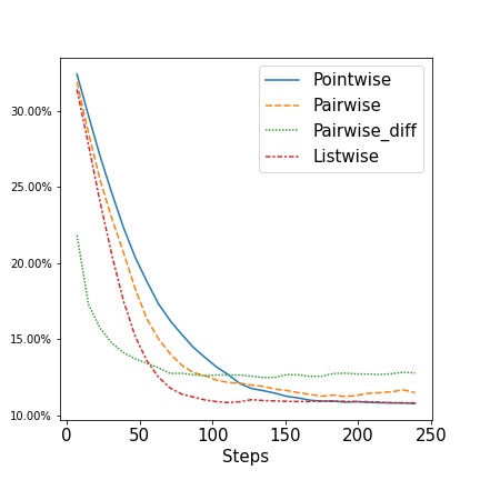
(a) Shortest path (Deg= 2)

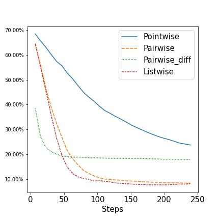
(b) Shortest path (Deg= 4)

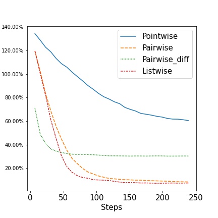
(c) Shortest path (Deg= 6)

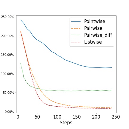
(d) Shortest path (Deg= 8)

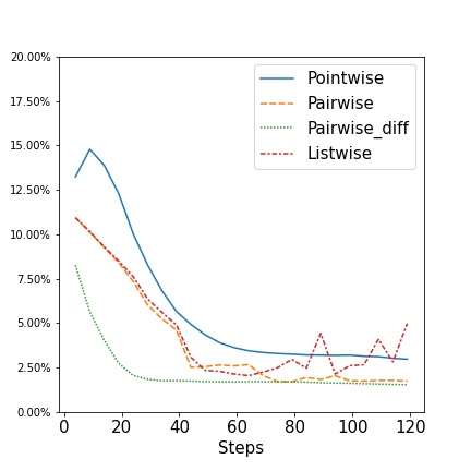
(e) Energy-1

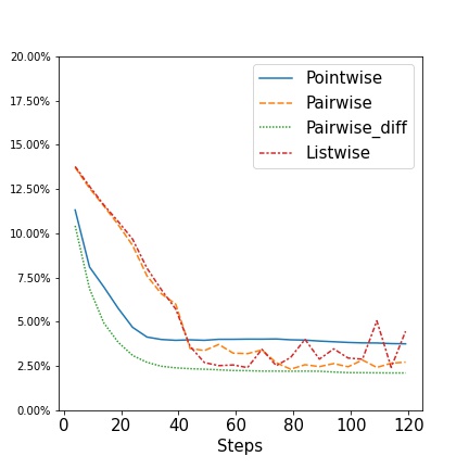
(f) Energy-2

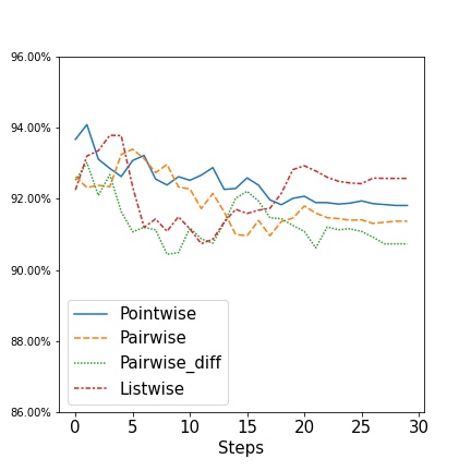
(g) Matching-1

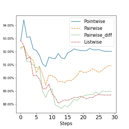
(h) Matching-2

Figure 1: Learning Curve. We show how the average regrets on validation dataset progress as the models learn.

4.5 Implementation

So far we define pointwise (6) pairwise (11), pairwise-difference (13) and listwise (16) ranking losses. As mentioned, the fundamentals of the LTR loss functions is to learn the partial ordering of $v\in S$. To construct and expand $S$, we use the strategy of Mulamba et al. (2021). The generic structure of the proposed algorithm is shown in Algorithm 1, which is a modified version of standard gradient descent algorithms for decision-focused learning problems. They proposed to initialise $S$ with all true optimal solutions. In Algorithm 1 $S$ is initialized by caching all the optimal solutions of the training instances in line 2. To expand $S$, they defined a hyperparameter $p_{solve}$, which is the probability of calling a optimization oracle to solve an instance during training. If an instance is solved, its solution is added to $S$. This is demonstrated in line 8 in Algorithm 1. Obviously with $p_{solve}=100\%$, Eq. (1) is solved for every $\hat{c}_{i}$ during training.

Table 1: Comparison of regret on three problem sets. We present average percentage regret of 10 runs.

	Pointwise	Pairwise	Pairwise-diff	Listwise	NCE	MAP	SPO	Blackbox	Twostage
Shortest Path Problem
Deg-1	15.45%	16.37%	16.00%	15.56%	23.63%	19.68%	15.51%	18.62%	15.45%
Deg-2	10.07%	10.74%	11.60%	10.41%	30.84%	14.15%	10.06%	13.26%	10.07%
Deg-4	19.27%	8.06%	17.89%	7.71%	65.10%	9.44%	7.98%	9.39%	10.44%
Deg-6	72.18%	9.27%	32.63%	8.29%	129.42%	9.45%	16.19%	9.69%	15.96%
Deg-8	178.16%	12.75%	61.80%	12.38%	242.30%	13.68%	33.75%	14.14%	28.50%
Energy Scheduling Problem
Energy-1	2.51%	1.65%	1.63%	1.67%	1.69%	1.59%	1.56%	1.54%	1.91%
Energy-2	2.83%	2.08%	2.04%	1.96%	2.23%	2.01%	1.93%	1.93%	2.46%
Bipartite Matching Problem
Matching-1	90.17%	88.80%	88.23%	88.49%	89.39%	89.13%	88.70%	90.09%	90.12%
Matching-2	89.86%	87.24%	85.87%	86.40%	85.31%	84.80%	85.79%	90.31%	89.42%

The distinctive feature of this proposed approach is that the loss function $L(\hat{c}_{i},c_{i})$ does not involve any argmin differentiation. So we can use standard automatic differentiation libraries and it can be run on GPU. Yet, it still considers the task loss of the downstream optimization problem. The part that can not be run on GPU is calling an optimization oracle to expand $S$.

5 Experiments

We analyze our approaches on a series of experiments. We consider three discrete combinatorial optimization problems. First, we briefly describe the experimental setups.

Shortest Path Problems.

We adopt this synthetic experiment from Elmachtoub & Grigas (2021). It is a shortest path problem in a $5\times 5$ grid, with the objective of going from the southwest corner of the grid to the northeast corner where the edges can go either north or east. The feature vectors are sampled from a multivariate Gaussian distribution. They generate the cost vector as per the following model

$$c_{ij}=\bigg{(}\frac{1}{\sqrt{p}}\big{(}Bx_{i}\big{)}+3\bigg{)}^{\text{Deg}}\epsilon_{i}^{j}$$ (17)

where $c_{ij}$ is the $j$-th component of cost vector $c_{i}$ and $B$ is the latent data generation matrix. Deg specifies the extent of model specification, the higher the value of Deg, the more it deviates from a linear model and the more errors there will be. We experiment with degree of $1,2,4,6\text{ and }8$. $\epsilon_{i}^{j}$ is a multiplicative noise that is sampled from $\text{U}(0.5,1.5)$. For each degree, we have 1000, 250 and 10,000 training, validation and test instances. The underlying model is a neural network without any hidden layer i.e. a regression model.

Energy-cost Aware Scheduling.

Next we consider the problem of energy-cost aware scheduling, adapted from CSPLib (Gent & Walsh, 1999), a library of constraint optimization problems. In energy-cost aware scheduling (Simonis et al., 1999), a given number of tasks, to be scheduled on a certain number of machines without violating the resource capacities of each machine. The goal of the optimization problem is to find the scheduling which would minimize the total energy consumption subject to the energy prices, which would be realized in the future. The prediction task is to predict the future energy prices using feature variables such as calendar attributes; day-ahead estimates of weather characteristics, forecasted energy-load, wind-energy production and prices. We take the energy price data from Ifrim et al. (2012). We study two instances named Energy-1 and Energy-2. The first one involves scheduling 3 tasks on 10 machines, whereas the other instance has 3 tasks and 15 machines.

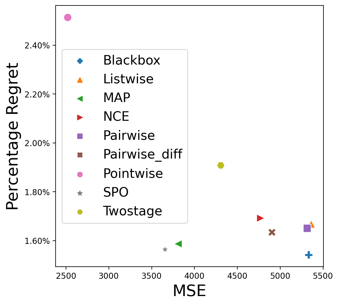
(a) Energy-1

(b) Energy-2

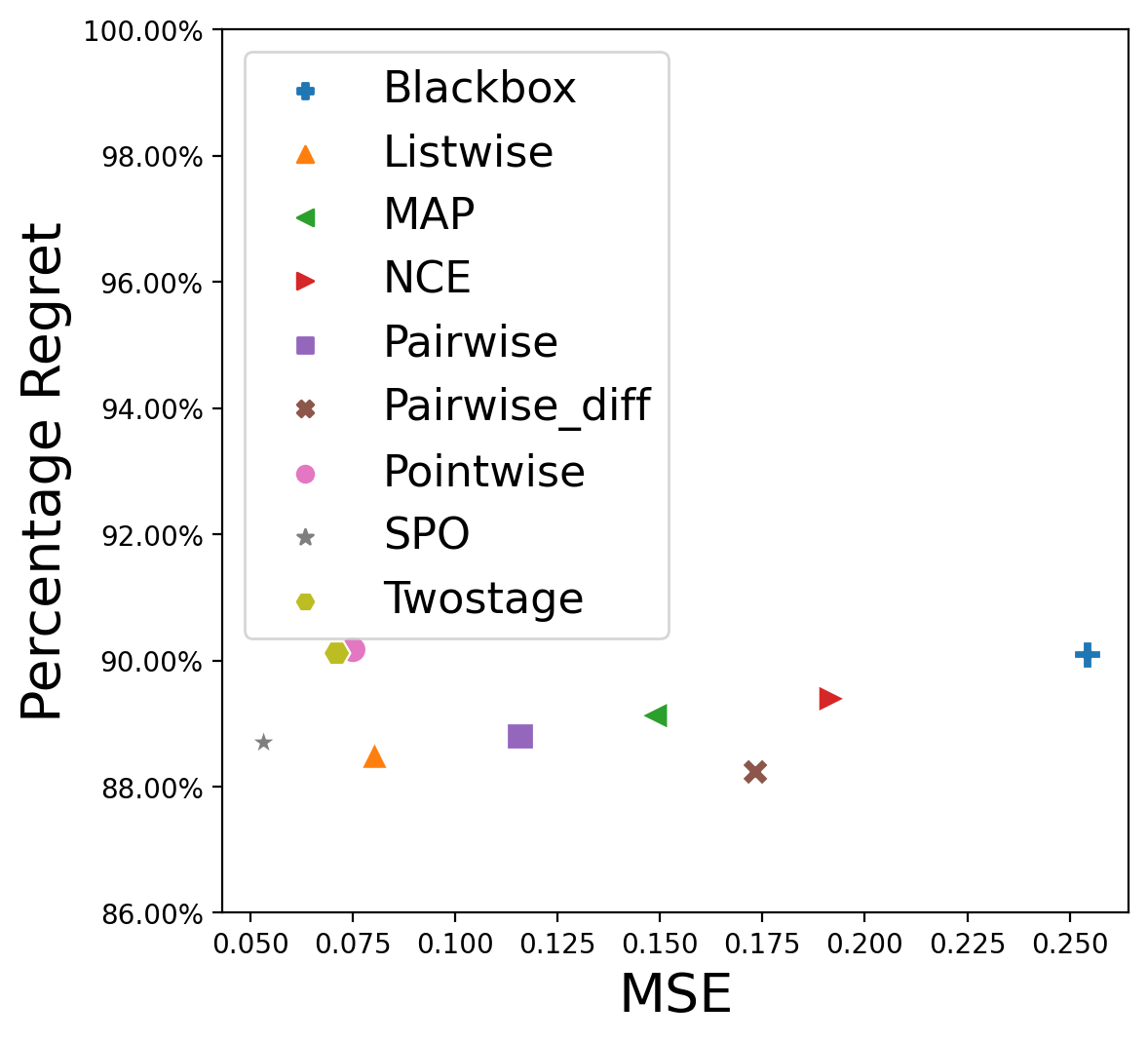
(c) Matching-1

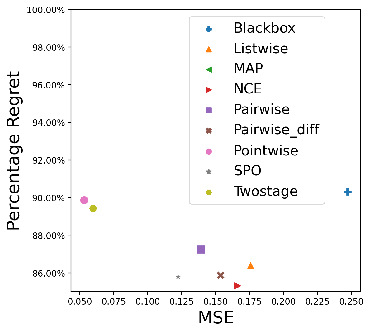
(d) Matching-2

Figure 2: MSE vs Regret trade-off

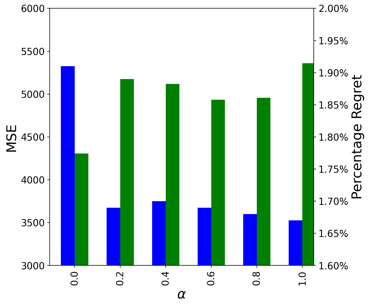
(a) Energy-1

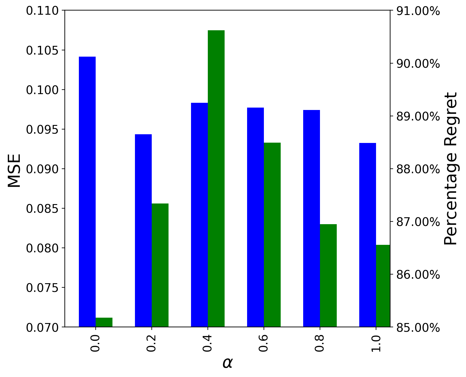
(b) Matching-1

Figure 3: Change of MSE and Regret with $\alpha$ as a tuning parameter. The green and blue bar present the MSE loss and percentage regret respectively.

Diverse Bipartite Matching.

We adopt this from Ferber et al. (2020) and Mulamba et al. (2021). The topologies are taken from the CORA citation network (Sen et al., 2008). We have 27 disjoint topologies and each of them is considered as an instance. The prediction task is to predict which edges are present. Each node has 1433 bag-of-words features. The feature of and edge is formed by concatenating features of the two corresponding nodes. The optimization task is to find the maximum matching after prediction. In the optimization task, diversity constraints ensures that there are some edges between papers of the same field as well as edges between papers of different fields. We study two instantiations with different degrees of diversity constraints (see Appendix for detail).

5.1 Experimental Results

Performance of surrogate loss functions.

In this section, we compare the quality of the rank based loss functions. As described in section 4, we train the neural network with respect to these loss functions. As our objective is to have lower regret, we consider the percentage regret ($\frac{f(v^{\star}(\hat{c}),c)-f(v^{\star}(c),c)}{f(v^{\star}(c),c)}$) as the evaluation metric. One way to know whether model training decreases the regret is to monitor the regret on the validation dataset. Figure 1 validates that by minimizing the surrogate losses, the neural network models learn to lower the regret. In the shortest path problem, overall, the listwise and pairwise loss functions perform better than the other two. The difference is more pronounced in higher degrees, where the linear model makes larger error. In the scheduling and matching experiments, the pairwise difference loss generalizes the best. The lowest regret of listwise loss is similar to pairwise difference, but its learning curve is less stable.

Next we compare the rank based loss functions with the SPO+ loss (Elmachtoub & Grigas, 2021), Blackbox backpropagation approach (Pogancic et al., 2020) and the NCE and MAP approach of Mulamba et al. (2021). We also include a two-stage baseline approach which is trained purely on MSE loss. We present average regret on test data of 10 independent trials in Table 1. We refer the readers to C to view the distribution of the regrets. For the shortest path problem, we again see the regret goes up with the degree parameter. This is expected as the degree parameter controls the magnitude of the errors of the linear model. For degree 4, 6 and 8, the listwise loss function produces the lowest regret. For lower two degrees, the pointwise and pairwise difference loss function produces low regret, but their regret jumps up at higher degrees. This is reasonable as their los functions include the absolute difference between the predicted and true solutions. Listwise loss comes second among all in Energy-2 and Matching-1. The pairwise difference loss has lowest regret in Matching-1 and its regret is competitive with the best loss function in these two problems. In all cases the pointwise loss function performs poorly, even worse than pure MSE (two-stage). The possible explanation is that its added penalty term is not always aligned with regret as discussed in section 4.2. Overall, Table 1 and Figure 1 indicate the performance of the parirwise difference loss is steady when the underlying predictive model is consistent with the data generation process, whereas the listwise loss is robust and reliable across all problem instances.

Table 2: Impact of $p_{solve}$ on per epoch training time and regret in Energy scheduling instances

		Pointwise		Pairwise		Pairwise-diff		Listwise
	$p_{solve}$	Regret	Time (s)	Regret	Time (s)	Regret	Time (s)	Regret	Time (s)
Energy-1	100%	2.12%	110	1.64%	110	1.63%	110	1.72%	100
	10%	2.51%	30	1.65%	30	1.61%	30	1.67%	25
Energy-2	100%	2.70%	130	2.05%	140	2.07%	140	1.99%	120
	10%	2.83%	40	2.08%	45	2.04%	45	1.96%	40

MSE vs Regret tradeoff.

The three problems we consider happen all to be integer linear programming (ILP) problems. As ILP problems are scale-invariant, the regret can be minimized even if the predictions are multiples of the actual values. In Figure 2, we show both MSE and regret of the predictions. In all cases we observe that the MSE loss of the pointwise loss is very low, comparable to minimizing MSE. But its regret is even higher than MSE, as seen before. The pairwise difference loss function has marginally better MSE than listwise and pairwise losses, showing little added gain from its more MSE-related formulation.

Combined Regression and Ranking Experiment.

The previous experiment reveals that although the performances of the ranking loss functions are comparable with the state of the art in terms of regret, their MSE loss remains high. In this experiment we will consider a convex combination of MSE loss and listwise ranking loss, inspired by  (Sculley, 2010) but formulated as a multi-task problem instead of sampling between the two losses:

$$\alpha L^{l}_{S}(\hat{c},c)+(1-\alpha)\mathbf{mse}(\hat{c},c)$$ (18)

The motivation behind this loss function is that we can control $\alpha$ as a tuning parameter. Clearly, $\alpha=0$ results in MSE loss whereas $\alpha=1$ results in listwise ranking loss. Figure 3 displays the impact $\alpha$ on the two scheduling instances. As hypothesised, we see MSE goes up and regret goes down as we increase $\alpha$. This experiment suggests it is possible to choose a value of $\alpha$ so that we sacrifice regret (problem-specific) to attain predictions with lower MSE (close to the true values).

Impact of $p_{solve}$.

The motivation behind ours (and Mulamba et al. (2021)) approach is reducing the number of times of the optimization problem is solved during training. In the next experiment, we show how $p_{solve}$ impacts the model training time. Lower values of $p_{solve}$ would make the training faster because of two reasons. Firstly, we have to call the optimization oracle few number of times. Secondly, the smaller cardinality means ranking loss would be computed on fewer datapoints.In Table 2 we report percentage regret and per epoch runtime of the four ranking loss functions for $p_{solve}=10\%\text{ and }100\%$ for the scheduling instances. We choose this problem because this is most difficult optimization problem among the three. Table 2 shows that in all cases, reducing $p_{solve}$ to 10% barely impacts regret for all except pointwise (which already performs worse). On the other hand, the efficiency gain in terms of runtime is significant.

6 Conclusion

We extend the approach of Mulamba et al. (2021), which introduces surrogate loss functions for decision-focused learning problems by caching a subset of feasible solutions. Motivated by their work, we frame the decision-focused learning problem as a learning to rank problem, where we train models to learn the partial ordering of the pool of feasible solutions. This generalizes their approach and inherits its nice properties of separating the solving from the loss computation. We also attempt to draw connections between the two-stage MSE loss and regret minimizing ranking losses. This stimulates a further cross fertilisation of the rich and more mature field of learning to rank with the relatively recent topic of decision-focused learning.

Appendix A Problem Specification

A.1 Shortest Path Problem

In this problem, we consider shortest path problem on $5\times 5$ a grid. The goal is to go from the southwest corner to the northeast corner, where we can go towards east or north. We model it as an LP problem.

$$\min_{x\geq 0}c^{\top}x$$

$$Ax=b$$

Where $A$ is the incidence matrix. The decision variable $x$ is binary vector whose entries would be 1 only if corresponding edge is selected for traversal. $b$ is 25 dimensional vector whose first entry is 1 and last entry is -1 and rest are 0. The constraint must be satisfied to go from the southwest corner to the northeast corner. With respect to the (predicted) cost vector $c\in\mathbb{R}^{|E|}$, the objective is to minimize the cost.

A.2 Energy-cost Aware Scheduling

In this problem $J$ is the set of tasks to be scheduled on $M$ number of machines maintaining resource requirement of $R$ resources. The tasks must be scheduled over $T$(= 48) set of equal length time periods. Each task $j$ is specified by its duration $d_{j}$, earliest start time $e_{j}$, latest end time $l_{j}$, power usage $p_{j}$.$u_{jr}$ is the resource usage of task $j$ for resource $r$ and $c_{mr}$ is the capacity of machine $m$ for resource $r$. Let $x_{jmt}$ be a binary variable which is 1 only if task $j$ starts at time $t$ on machine $m$. If $c_{t}$ is the (predicted) energy price at timeslot $t$, the objective is to minimize the following formulation of total energy cost. Then the problem can be formulated as the following MILP:

$$\min_{x_{jmt}} \sum_{j\in J}\sum_{m\in M}\sum_{t\in T}x_{jmt}\Big{(}\sum_{t\leq t^{\prime}<t+d_{j}}p_{j}c_{t^{\prime}}\Big{)}$$

subject to $$\sum_{m\in M}\sum_{t\in T}x_{jmt}=1\ ,\forall_{j\in J}$$

$$x_{jmt}=0\ \ \forall_{j\in J}\forall_{m\in M}\forall_{t<e_{j}}$$

$$x_{jmt}=0\ \ \forall_{j\in J}\forall_{m\in M}\forall_{t+d_{j}>l_{j}}$$

$$\sum_{j\in J}\sum_{t-d_{j}<t^{\prime}\leq t}x_{jmt^{\prime}}u_{jr}\leq c_{mr},\forall_{m\in M}\forall_{r\in R}\forall_{t\in T}$$

The first constraint ensures each task is scheduled only once. The next constraints ensure the task scheduling abides by earliest start time and latest end time constraints. The final constraint is to respect the resource requirement of the machines.

A.3 Diverse Bipartite Matching

We adapt this from Ferber et al. (2020). in this problem 100 nodes representing scientific publications are split into two sets of 50 nodes $N_{1}$ and $N_{2}$. A (predicted) reward matrix $c$ indicates the likelihood that a link between each pair of nodes from $N_{1}$ to $N_{2}$ exists. Finally a indicator $m_{i,j}$ is $0$ if article $i$ and $j$ share the same subject field, and $0$ otherwise $\forall i\in N_{1},j\in N_{2}$. Let $p\in[0,1]$ be the rate of pair sharing their field in a solution and $q\in[0,1]$ the rate of unrelated pairs, the goal is to match as much nodes in $N_{1}$ with at most one node in $N_{2}$ by selecting edges which maximizes the sum of rewards under similarity and diversity constraints. Formally:

$$\begin{array}[]{lll}\max_{x}&\sum_{i,j}c_{i,j}x_{i,j}&\\ \text{ subject to }&\sum_{j}x_{i,j}\leq 1&\forall i\in N_{1}\\ &\sum_{i}x_{i,j}\leq 1&\forall j\in N_{2}\\ &\sum_{i.j}m_{i,j}x_{i,j}\geq p\sum_{i,j}x_{i,j}&\\ &\sum_{i.j}(1-m_{i,j})x_{i,j}\geq q\sum_{i,j}x_{i,j}\\ &x_{i,j}\in\{0,1\}&\forall i\in N_{1},j\in N_{2}\\ \end{array}$$

In our experiments, we considered two variations of this problem with $p=q=$ being $25\%$ and $5\%$, respectively named Matching-1 and Matching-2.

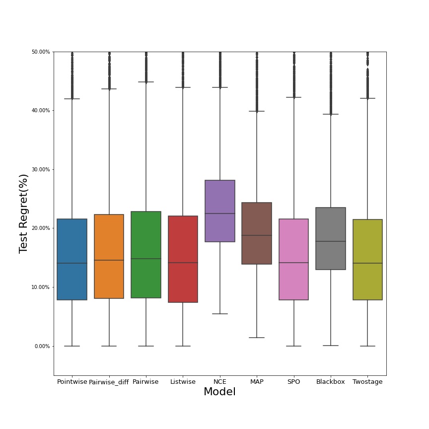
(a) Shortest path (Deg= 1)

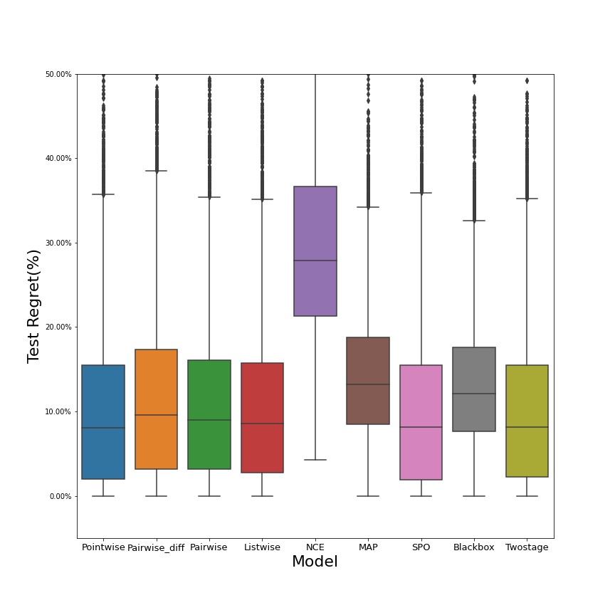
(b) Shortest path (Deg= 2)

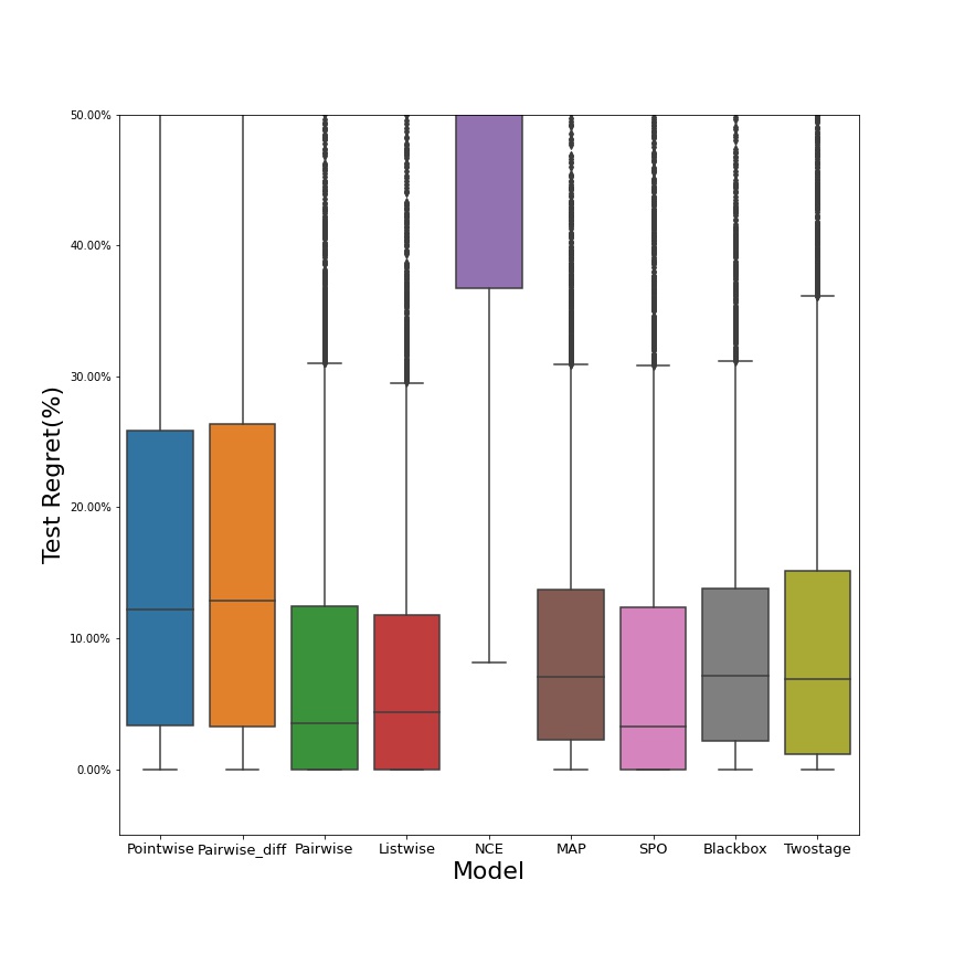
(c) Shortest path (Deg= 4)

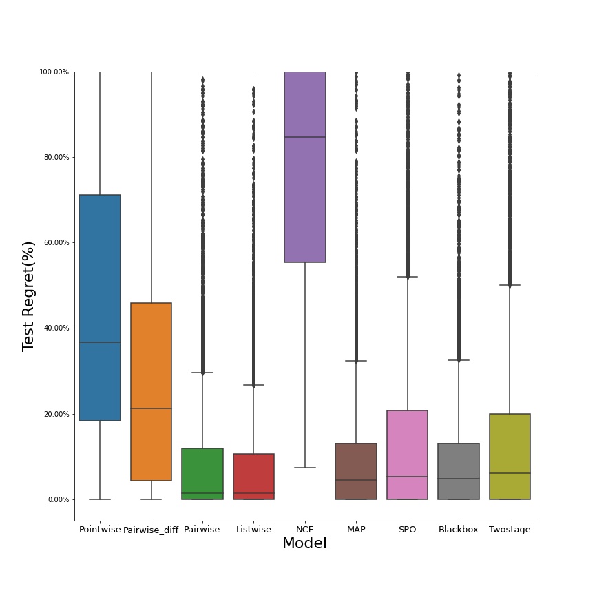
(d) Shortest path (Deg= 6)

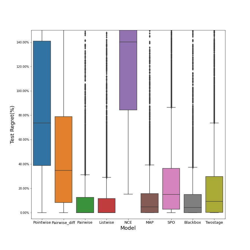
(e) Shortest path (Deg= 8)

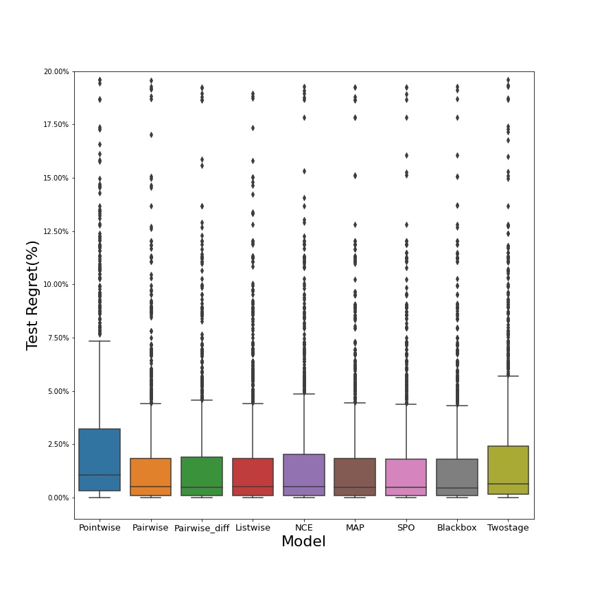
(f) Energy-1

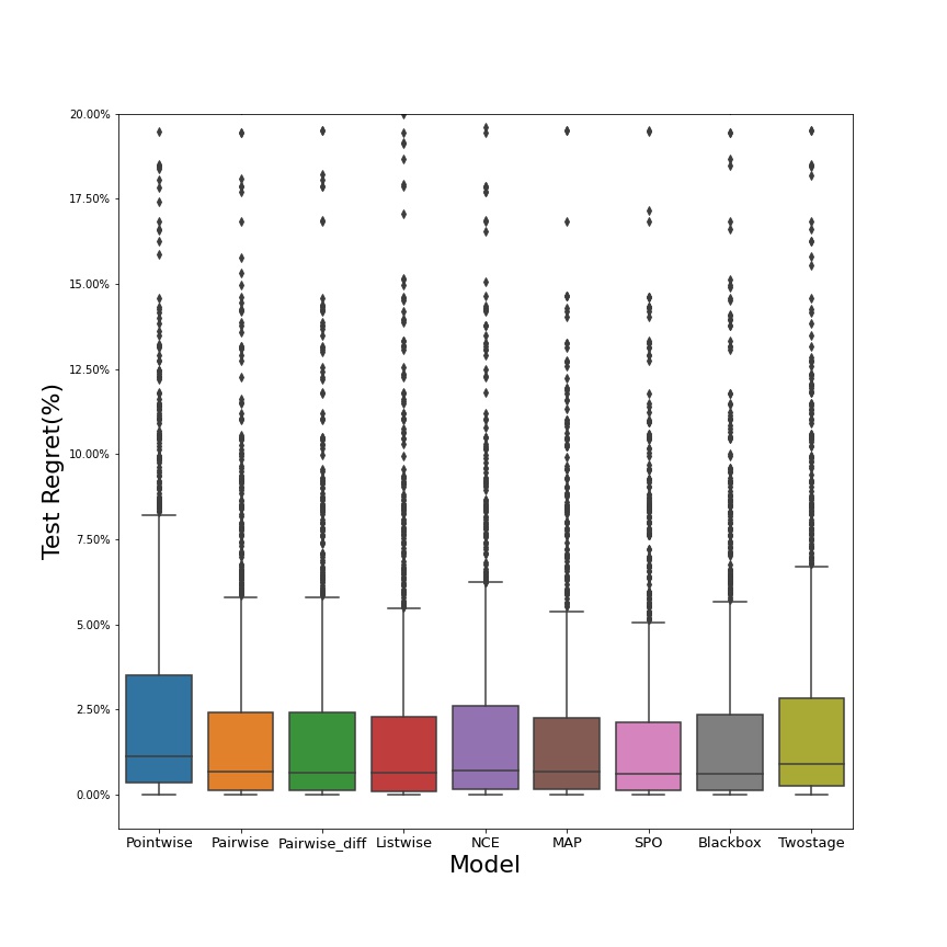
(g) Energy-2

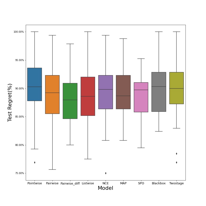
(h) Matching-1

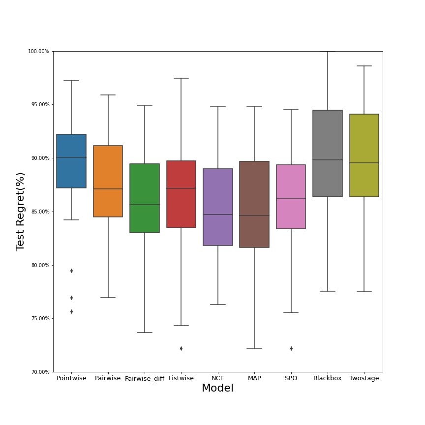
(i) Matching-2

Figure 4: Boxplot

Appendix B Hyperparameter Configuration

To reproduce the result reported in this paper use the hyperparameter settings as described in Table 3.

Table 3: Details of hyperparameters for reproducing the result

		Shortest Path Problem
		Deg-1	Deg-2	Deg-4	Deg-6	Deg-8
Pointwise	learning rate	0.8	0.8	0.8	0.8	0.8
Pairwise	learning rate	0.1	0.1	0.1	0.1	0.1
	margin	1.0	0.1	0.1	0.1	0.1
Listwise	learning rate	0.1	0.1	0.1	0.1	0.1
	temperature	1.0	0.1	0.05	0.05	0.05
Pairwise-difference	learning rate	0.1	0.1	0.1	0.5	0.5
NCE	learning rate	0.5	0.5	0.5	0.5	0.5
MAP	learning rate	0.05	0.05	0.05	0.7	0.7
SPO	learning rate	0.1	0.5	0.5	0.5	0.1
Blackbox	learning rate	0.5	0.5	0.5	0.5	0.5
	displace parameter	1.	1.	1.	1.	1.
Twostage	learning rate	0.5	0.5	0.1	0.5	0.5
		Energy Scheduling			Bipartite Matching
		Energy-1	Energy-2		Matching-1	Matching-2
Pointwise	learning rate	0.9	0.5		0.01	0.01
Pairwise	learning rate	0.1	0.1		0.001	0.01
	margin	100	100		0.2	1.0
Listwise	learning rate	0.1	0.1		0.005	0.01
	temperature	1.0	1.0		0.01	1.0
Pairwise-difference	learning rate	0.5	0.5		0.01	0.01
NCE	learning rate	0.5	0.5		0.001	0.01
MAP	learning rate	0.5	0.5		0.001	0.01
SPO	learning rate	0.9	0.9		0.01	0.01
Blackbox	learning rate	0.1	0.1		0.01	0.01
	displace parameter	0.001	0.1		$10^{-5}$	0.001
Twostage	learning rate	0.7	0.7		0.01	0.01

Appendix C Distribution of the regret of the predictions

In Table 1, we report only the average regret of all the instances over 10 independent trails. In Figure fig:boxplot, we show the distributions of the regret across all the test instances with box-plots for the three problems.

References

- Amos & Kolter (2017) Amos, B. and Kolter, J. Z. Optnet: Differentiable optimization as a layer in neural networks. In International Conference on Machine Learning, pp. 136–145. PMLR, 2017.
- Burges et al. (2005) Burges, C., Shaked, T., Renshaw, E., Lazier, A., Deeds, M., Hamilton, N., and Hullender, G. Learning to rank using gradient descent. In Proceedings of the 22nd international conference on Machine learning, pp. 89–96, 2005.
- Cao et al. (2007) Cao, Z., Qin, T., Liu, T.-Y., Tsai, M.-F., and Li, H. Learning to rank: from pairwise approach to listwise approach. In Proceedings of the 24th international conference on Machine learning, pp. 129–136, 2007.
- Demirović et al. (2019) Demirović, E., Stuckey, P. J., Bailey, J., Chan, J., Leckie, C., Ramamohanarao, K., and Guns, T. An investigation into prediction + optimisation for the knapsack problem. In Rousseau, L.-M. and Stergiou, K. (eds.), Integration of Constraint Programming, Artificial Intelligence, and Operations Research, pp. 241–257, Cham, 2019. Springer International Publishing. ISBN 978-3-030-19212-9.
- Elmachtoub & Grigas (2021) Elmachtoub, A. N. and Grigas, P. Smart “predict, then optimize”. Management Science, 2021.
- Ferber et al. (2020) Ferber, A. M., Wilder, B., Dilkina, B., and Tambe, M. Mipaal: Mixed integer program as a layer. In The Thirty-Fourth AAAI Conference on Artificial Intelligence, AAAI 2020, The Thirty-Second Innovative Applications of Artificial Intelligence Conference, IAAI 2020, The Tenth AAAI Symposium on Educational Advances in Artificial Intelligence, EAAI 2020, New York, NY, USA, February 7-12, 2020, pp. 1504–1511. AAAI Press, 2020.
- Gent & Walsh (1999) Gent, I. P. and Walsh, T. Csplib: a benchmark library for constraints. In International Conference on Principles and Practice of Constraint Programming, pp. 480–481. Springer, 1999.
- Gutmann & Hyvärinen (2010) Gutmann, M. and Hyvärinen, A. Noise-contrastive estimation: A new estimation principle for unnormalized statistical models. In Proceedings of the Thirteenth International Conference on Artificial Intelligence and Statistics, pp. 297–304, 2010.
- Ifrim et al. (2012) Ifrim, G., O’Sullivan, B., and Simonis, H. Properties of energy-price forecasts for scheduling. In International Conference on Principles and Practice of Constraint Programming, pp. 957–972. Springer, 2012.
- Joachims (2002) Joachims, T. Optimizing search engines using clickthrough data. In Proceedings of the Eighth ACM SIGKDD International Conference on Knowledge Discovery and Data Mining, July 23-26, 2002, Edmonton, Alberta, Canada, pp. 133–142. ACM, 2002.
- Karatzoglou et al. (2013) Karatzoglou, A., Baltrunas, L., and Shi, Y. Learning to rank for recommender systems. In Proceedings of the 7th ACM Conference on Recommender Systems, pp. 493–494, 2013.
- Kotary et al. (2021) Kotary, J., Fioretto, F., Hentenryck, P. V., and Wilder, B. End-to-end constrained optimization learning: A survey. In Proceedings of the Thirtieth International Joint Conference on Artificial Intelligence, volume 5, pp. 4475–4482, 2021.
- Kotary et al. (2021) Kotary, J., Fioretto, F., Van Hentenryck, P., and Zhu, Z. End-to-end learning for fair ranking systems. arXiv preprint arXiv:2111.10723, 2021.
- Li et al. (2007) Li, P., Wu, Q., and Burges, C. Mcrank: Learning to rank using multiple classification and gradient boosting. Advances in neural information processing systems, 20:897–904, 2007.
- Liu (2011) Liu, T.-Y. Learning to rank for information retrieval. 2011.
- Mandi & Guns (2020) Mandi, J. and Guns, T. Interior point solving for lp-based prediction+optimisation. In Larochelle, H., Ranzato, M., Hadsell, R., Balcan, M. F., and Lin, H. (eds.), Advances in Neural Information Processing Systems, volume 33, pp. 7272–7282. Curran Associates, Inc., 2020.
- Mandi et al. (2020) Mandi, J., Demirović, E., Stuckey, P. J., and Guns, T. Smart predict-and-optimize for hard combinatorial optimization problems. Proceedings of the AAAI Conference on Artificial Intelligence, 34(02):1603–1610, Apr. 2020.
- Mulamba et al. (2021) Mulamba, M., Mandi, J., Diligenti, M., Lombardi, M., Bucarey, V., and Guns, T. Contrastive losses and solution caching for predict-and-optimize. In Zhou, Z.-H. (ed.), Proceedings of the Thirtieth International Joint Conference on Artificial Intelligence, IJCAI-21, pp. 2833–2840. International Joint Conferences on Artificial Intelligence Organization, 8 2021.
- Niepert et al. (2021) Niepert, M., Minervini, P., and Franceschi, L. Implicit mle: Backpropagating through discrete exponential family distributions. In Ranzato, M., Beygelzimer, A., Dauphin, Y., Liang, P., and Vaughan, J. W. (eds.), Advances in Neural Information Processing Systems, volume 34, pp. 14567–14579. Curran Associates, Inc., 2021.
- Pogancic et al. (2020) Pogancic, M. V., Paulus, A., Musil, V., Martius, G., and Rolinek, M. Differentiation of blackbox combinatorial solvers. In 8th International Conference on Learning Representations, ICLR 2020, Addis Ababa, Ethiopia, April 26-30, 2020, 2020.
- Sculley (2010) Sculley, D. Combined regression and ranking. In Proceedings of the 16th ACM SIGKDD International Conference on Knowledge Discovery and Data Mining, KDD ’10, pp. 979–988. Association for Computing Machinery, 2010. ISBN 9781450300551.
- Sen et al. (2008) Sen, P., Namata, G., Bilgic, M., Getoor, L., Galligher, B., and Eliassi-Rad, T. Collective classification in network data. AI Magazine, 29(3):93, Sep. 2008.
- Simonis et al. (1999) Simonis, H., O’Sullivan, B., Mehta, D., Hurley, B., and Cauwer, M. D. CSPLib problem 059: Energy-cost aware scheduling. http://www.csplib.org/Problems/prob059, 1999.
- Wilder et al. (2019) Wilder, B., Dilkina, B., and Tambe, M. Melding the data-decisions pipeline: Decision-focused learning for combinatorial optimization. In The Thirty-Third AAAI Conference on Artificial Intelligence, AAAI 2019, The Thirty-First Innovative Applications of Artificial Intelligence Conference, IAAI 2019, The Ninth AAAI Symposium on Educational Advances in Artificial Intelligence, EAAI 2019, Honolulu, Hawaii, USA, January 27 - February 1, 2019, pp. 1658–1665. AAAI Press, 2019.
- Xuan & Monperrus (2014) Xuan, J. and Monperrus, M. Learning to combine multiple ranking metrics for fault localization. In 2014 IEEE International Conference on Software Maintenance and Evolution, pp. 191–200. IEEE, 2014.