Membership Inference Attacks From First Principles

Abstract

A membership inference attack allows an adversary to query a trained machine learning model to predict whether or not a particular example was contained in the model’s training dataset. These attacks are currently evaluated using average-case “accuracy” metrics that fail to characterize whether the attack can confidently identify any members of the training set. We argue that attacks should instead be evaluated by computing their true-positive rate at low (e.g., $\leq 0.1\%$) false-positive rates, and find most prior attacks perform poorly when evaluated in this way. To address this we develop a Likelihood Ratio Attack (LiRA) that carefully combines multiple ideas from the literature. Our attack is 10$\times$ more powerful at low false-positive rates, and also strictly dominates prior attacks on existing metrics.

I Introduction

Neural networks are now trained on increasingly sensitive datasets, and so it is necessary to ensure that trained models are privacy-preserving. In order to empirically verify if a model is in fact private, membership inference attacks [60] have become the de facto standard [63, 42] because of their simplicity. A membership inference attack receives as input a trained model and an example from the data distribution, and predicts if that example was used to train the model.

Unfortunately as noted by recent work [44, 69], many prior membership inference attacks use an incomplete evaluation methodology that considers average-case success metrics (e.g., accuracy or ROC-AUC) that aggregate an attack’s accuracy over an entire dataset and over all detection thresholds [63, 56, 70, 61, 6, 54, 54, 34, 35, 57, 45, 52, 55, 26, 66, 33, 18]. However, privacy is not an average case metric, and should not be evaluated as such [65]. Thus, while existing membership inference attacks do appear effective when evaluated under this average-case methodology, we make the case they do not actually effectively measure the worst-case privacy of machine learning models.

Contributions. In this paper we re-examine the problem statement of membership inference attacks from first principles. We first argue that membership inference attacks should be evaluated by considering their true-positive rate (TPR) at low false-positive rates (FPR). This objective of designing methods around low false-positive rates is typical in many areas of computer security [31, 49, 41, 27, 28, 21], and for similar reasons it is the right metric here. If a membership inference attack can reliably violate the privacy of even just a few users in a sensitive dataset, it has succeeded. And conversely, an attack that only unreliably achieves high aggregate attack success rate should not be considered successful.

When evaluated this way, we find most prior attacks fail in the low false-positive rate regime. Furthermore, aggregate metrics (e.g., AUC) are often uncorrelated with low FP success rates. For example the attack of Yeom et al. [70] has a high accuracy ($59.5\%$) yet fails completely at low FPRs, and the attack of Long et al. [36] has a much lower accuracy ($53.5\%$) but achieves higher success rates at low FPRs.

We develop a Likelihood Ratio Attack (LiRA) that succeeds $10\times$ more often than prior work at low FPRs—but still strictly dominates prior attacks on aggregate metrics introduced previously. Our attack combines per-example difficulty scores [56, 68, 37] with a principled and well-calibrated Gaussian likelihood estimate. Figure 1 shows the success rate of our attack on a log-scale Receiver Operating Characteristic (ROC) curve [59], comparing the ratio of true-positives to false-positives. We perform an extensive experimental evaluation to understand each of the factors that contribute to our attack’s success, and release our open source code.

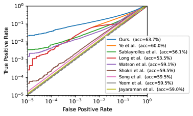
Figure 1: Comparing the true-positive rate vs. false-positive rate of prior membership inference attacks reveals a wide gap in effectiveness. An attack’s average accuracy is not indicative of its performance at low FPRs. By extending on the most effective ideas, we improve membership inference attacks by $10\times$, for a non-overfit CIFAR-10 model (92% test accuracy).

Future work will need to re-examine many questions that have been studied using prior, much less effective, membership inference attacks. Attacks that use less information (e.g., label-only attacks [6, 54, 34]) may or may not achieve high success rate at low false-positive rates; algorithms previously seen as “private” because they resist prior attacks might be vulnerable to our new attack; and old defenses dismissed as ineffective might be able to defend against these new stronger attacks.

II Background

We begin with a background that will be familiar to readers knowledgeable of machine learning privacy.

II-A Machine learning notation

A classification neural network $f_{\theta}:\mathcal{X}\to[0,1]^{n}$ is a learned function that maps some input data sample $x\in\mathcal{X}$ to an $n$-class probability distribution; we let $f(x)_{y}$ denote the probability of class $y$. Given a dataset $D$ sampled from some underlying distribution $\mathbb{D}$, we write $f_{\theta}\leftarrow\mathcal{T}(D)$ to denote that the neural network $f$ parameterized with weights $\theta$ is learned by running the training algorithm $\mathcal{T}$ on the training set $D$. Neural networks are trained via stochastic gradient descent [32] to minimize some loss function $\ell$:

$$\theta_{i+1}\leftarrow\theta_{i}-\eta\sum_{(x,y)\in B}\nabla_{\theta}\ell(f_{\theta_{i}}(x),y)$$ (1)

Here, $B$ is a batch of random training examples from $D$, and $\eta$ is the learning rate, a small constant. For classification tasks, the most common loss function is the cross-entropy loss:

$$\ell(f_{\theta}(x),y)=-\log(f_{\theta}(x)_{y})\;.$$

When the weights $\theta$ are clear from context, we will simply write a trained model as $f$. At times it will be useful to view a model $f$ as a function $f(x)=\sigma(z(x))$, where $z:\mathcal{X}\to\mathbb{R}^{n}$ returns the feature outputs of the network, followed by a softmax normalization layer $\sigma(z)=[\frac{e^{z_{1}}}{\sum_{i}e^{z_{i}}},\dots,\frac{e^{z_{n}}}{\sum_{i}e^{z_{i}}}]$.

Training neural networks that reach $100\%$ training accuracy is easy—running the gradient descent from Equation 1 on any sufficiently sized neural network eventually achieves this goal [72]. The difficulty is in training models that generalize to an unseen test set $D_{\text{test}}\leftarrow\mathbb{D}$ drawn from the same distribution. There are a number of techniques to increase the generalization ability of neural networks (augmentations [7, 67, 73], weight regularization [30], tuned learning rates [23, 38]). For the remainder of this paper, all models we train use state-of-the-art generalization-enhancing techniques. This makes our analysis much more realistic than prior work, which often uses models with 2–5$\times$ higher error rates than our models.

II-B Training data privacy

Neural networks must not leak details of their training datasets, particularly when used in privacy-sensitive scenarios [5, 13]. The field of training data privacy constructs attacks that leak data, develops techniques to prevent memorization, and measures the privacy of proposed defenses.

Privacy attacks

There are various forms of attacks on the privacy of training data. Training data extraction [4] is an explicit attack where an adversary recovers individual examples used to train the model. In contrast, model inversion attacks recover aggregate details of particular sub-classes instead of individual training examples [16]. Finally, property inference attacks aim at inferring non-trivial properties of the training dataset. For example, a classifier trained on bitcoin logs can reveal whether or not the machines that generated the logs were patched for Meltdown and Spectre [17].

We focus on a more fundamental attack that predicts if a particular example is part of a training dataset. First explored as tracing attacks [22, 59, 11, 12] on medical datasets, they were exended to machine learning models as membership inference attacks [60]. In these settings, being able to reliably (with high precision) identify a few users as being contained in sensitive medical datasets is itself a privacy violation [22]—even if this is done with low recall. Further, membership inference attacks are the foundation of stronger extraction attacks [3, 4], and in order to be used in this way must again have exceptionally high precision.

Theory of memorization

The ability to perform membership inference is directly tied to a model’s ability to memorize individual data points or labels. Zhang et al. [72] demonstrated that standard neural networks can memorize entirely randomly labeled datasets. A recent line of work initiated by Feldman [14] shows both theoretically and empirically that some amount of memorization may be necessary to achieve optimal generalization [15, 2].

Privacy-preserving training

The most widely deployed technique to make neural networks private is to make the learning process differentially private [10]. This can be done in various ways—for example by modifying the SGD algorithm [64, 1], or by aggregating results from a model ensemble [50]. Independent from differential privacy based defenses, there are other heuristic techniques (that is, without a formal proof of privacy) that have been developed to improve the privacy of machine learning models [45, 26]. Unfortunately, many of these have been shown to be vulnerable to more advanced forms of attack [6, 61].

Measuring training data privacy

Given a particular training scheme, a final direction of work aims to answer the question “how much privacy does this scheme offer?” Existing techniques often work by altering the training pipeline, either by injecting outlier canaries [3], or using poisoning to search for worst-case memorization [24, 47]. While these techniques give increasingly strong measurements of a trained model’s privacy, the fact that they require modifying the training pipeline creates an up-front cost to deployment. As a result, by far the most common technique used to audit machine learning models is to just use a membership inference attack. Existing membership inference attack libraries (see, e.g., Song and Marn [63], Murakonda and Shokri [42]) form the basis for most production privacy analysis [63], and it is therefore critical that they accurately assess the privacy of machine learning models.

III Membership Inference Attacks

The objective of a membership inference attack (MIA) [60] is to predict if a specific training example was, or was not, used as training data in a particular model. This makes MIAs the simplest and most widely deployed attack for auditing training data privacy. It is thus important that they can reliably succeed at this task. This section formalizes the membership inference attack security game (§III-A), and introduces our membership inference evaluation methodology (§III-B).

III-A Definitions

We define membership inference via a standard security game inspired by Yeom et al. [70] and Jayaraman et al. [25].

Definition 1 (Membership inference security game).

The game proceeds between a challenger $\mathcal{C}$ and an adversary $\mathcal{A}$:

1. The challenger samples a training dataset $D\leftarrow\mathbb{D}$ and trains a model $f_{\theta}\leftarrow\mathcal{T}(D)$ on the dataset $D$.

2. The challenger flips a bit $b$, and if $b=0$, samples a fresh challenge point from the distribution $(x,y)\leftarrow\mathbb{D}$ (such that $(x,y)\notin D$). Otherwise, the challenger selects a point from the training set $(x,y)\leftarrow^{\$}D$.

3. The challenger sends $(x,y)$ to the adversary.

4. The adversary gets query access to the distribution $\mathbb{D}$, and to the model $f_{\theta}$, and outputs a bit $\hat{b}\leftarrow\mathcal{A}^{\mathbb{D},f}(x,y)$.

5. Output 1 if $\hat{b}=b$, and 0 otherwise.

For simplicity, we will write $\mathcal{A}(x,y)$ to denote the adversary’s prediction on the sample $(x,y)$ when the distribution $\mathbb{D}$ and model $f$ are clear from context.

Note that this game assumes that the adversary is given access to the underlying training data distribution $\mathbb{D}$; while some attacks do not make use of this assumption [70], many attacks require query-access to the distribution in order to train “shadow models” [60] (as we will describe). The above game also assumes that the adversary is given access to both a training example and its ground-truth label.

Instead of outputting a “hard prediction”, all the attacks we consider output a continuous confidence score, which is then thresholded to yield a membership prediction. That is,

$$\mathcal{A}(x,y)=\mathbbm{1}[\mathcal{A}^{\prime}(x,y)>\tau]$$

where $\mathbbm{1}$ is the indicator function, $\tau$ is some tunable decision threshold, and $\mathcal{A}^{\prime}$ outputs a real-valued confidence score.

A first membership inference attack. For illustrative purposes, we begin by considering a very simple membership inference attack (due to Yeom et al. [70]). This attack relies on the observation that, because machine learning models are trained to minimize the loss of their training examples (see Equation 1), examples with lower loss are on average more likely to be members of the training data. Formally, the LOSS membership inference attack defines

$$\mathcal{A}_{\text{loss}}(x,y)=\mathbbm{1}[-\ell(f(x),y)>\tau]\;.$$

III-B Evaluating membership inference attacks

Prior work lays out several strategies to determine the effectiveness of a membership inference attack, i.e., how to measure the adversary’s success in Definition 1. We now show that existing evaluation methodologies fail to characterize whether an attack succeeds at confidently predicting membership. We thus propose a more suitable evaluation procedure.

As a running example for the remainder of this section, we train a standard CIFAR-10 [29] ResNet [19] to 92% test accuracy by training it on half of the dataset (i.e., $25{,}000$ examples)—leaving another $25{,}000$ examples for evaluation as non-members. While this dataset is not sensitive, it serves as a strong baseline for understanding properties of machine learning models in general. We train this model using standard techniques to reduce overfitting, including weight decay [30], train-time augmentations [7], and early stopping. As a result, this model has only a $8\%$ train-test accuracy gap.

Balanced Attack Accuracy. The simplest method to evaluate attack efficacy is through a standard “accuracy” metric that measures how often an attack correctly predicts membership on a balanced dataset of members and non-members [60, 70, 56, 46, 61, 6, 66, 33, 18, 68].

Definition 2.

The balanced attack accuracy of a membership inference attack $\mathcal{A}$ in Definition 1 is defined as

$$\Pr_{x,y,f,b}[\mathcal{A}^{\mathbb{D},f}(x,y)=b].$$

Even though balanced accuracy is used in many papers to evaluate membership inference attacks, we argue that this metric is inherently inadequate for multiple reasons:

• Balanced accuracy is symmetric. That is, the metric assigns equal cost to false-positives and to false-negatives. However, in practice, adversaries often only care about one of these two sources of errors. For example, when a membership inference attack is used in a training data extraction attack [4], false negatives are benign (some data will not be successfully extracted) whereas false-positives directly reduce the utility of the attack.

• Balanced accuracy is an average-case metric, but this is not what matters in security. Consider comparing two attacks. Attack A perfectly targets a known subset of $0.1\%$ of users, but succeeds with a random $50\%$ chance on the rest. Attack B succeeds with $50.05\%$ probability on any given user. On average, these two attacks have the same attack success rate (and thus the same balanced accuracy). However, the second attack is practically useless, while the first attack is exceptionally potent.

We now illustrate how exactly these issues arise for the simple LOSS attack described above. For our CIFAR-10 model, this attack’s balanced accuracy is $60\%$. This is (much) better than random guessing, and so one might reasonably conclude that the attack is useful and practically worrying.

However, this attack completely fails at confidently identifying any members! Let’s examine for the moment the $1\%$ of samples from the CIFAR-10 dataset with lowest losses $\ell(f(x),y)$. These are the samples where the attack is most confident that they are members. Yet, on this subset, the attack is only correct $48\%$ of the time (worse than random guessing). In contrast, for the 1% samples with highest loss (confident non-members), the attack is correct $100\%$ of the time. Thus, the LOSS attack is actually a strong non-membership inference attack, and is practically useless at inferring membership. An attack with the symmetrical property (i.e., the attack confidently identifies members, but not non-members) is a much stronger attack on privacy, yet it achieves the same balanced accuracy.

ROC Analysis. Instead of the balanced accuracy, we should thus consider metrics that emphasize positive predictions (i.e., membership guesses) over negative (non-membership) predictions. A natural choice is to consider the tradeoff between the true-positive rate (TPR) and false-positive rate (FPR). Intuitively, an attack should maximize the true-positive rate (many members are identified), while incurring few false-positives (incorrect membership guesses). We prefer this to a precision/recall analysis because TPR/FPR is independent of the (often unknown) prevalence of members in the population.

The TPR/FPR tradeoff is fully characterized by the Receiver Operating Characteristic (ROC) curve, which compares the attack’s TPR and FPR for all possible choices of the decision threshold $\tau$. In Figure 2(a), we show the ROC curve for the LOSS attack. The attack fails to achieve a TPR better than random chance at any FPR below $20\%$—it is therefore ineffective at confidently breaching the privacy of its members.

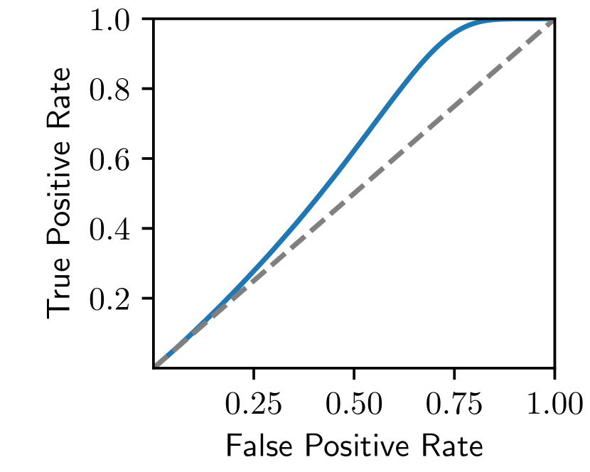
(a) linear scale

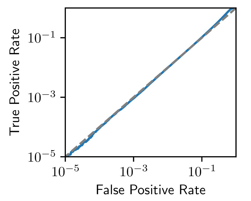
(b) log scale

Figure 2: ROC curve for the LOSS baseline membership inference attack, shown with both linear scaling (left), also and log-log scaling (right) to emphasize the low-FPR regime.

Prior papers that do report ROC curves summarize them by the AUC (Area Under the Curve) [57, 39, 20, 68, 69, 43]. However, as we can see from the curves above, the AUC is not an appropriate measure of an attack’s efficacy, since the AUC averages over all false-positive rates, including high error rates that are irrelevant for a practical attack. The TPR of an attack when the FPR is above 50% is not meaningfully useful, yet this regime accounts for more than half of its AUC score.

To illustrate, consider our hypothetical Attack A from earlier that confidently identifies 0.1% of members, but makes no confident predictions for any other samples. This attack perfectly breaches the privacy of some members, but has an AUC $\approx 51\%$—lower than the AUC of the weak LOSS attack.

True-Positive Rate at Low False-Positive Rates. Our recommended evaluation of membership inference attacks is thus to report an attack’s true-positive rate at low false-positive rates.

Prior work occasionally reports true-positive rates at moderate false-positive rates (or reports precision/recall values that can be converted into TPR/FPR rates if the prevalence is known). For example, Shokri et al. [60] frequently reports that the “recall is almost 1” however there is a meaningful FPR difference between a recall of 1.0 and 0.999. Other works consistently report precision/recall values, but for equivalent false-positive rates between $3\%$ and $40\%$, which we argue is too high to be practically meaningful.

In this paper, we argue for studying the extremely low false-positive regime. We do this by (1) reporting full ROC curves in logarithmic scale (see Figure 2(b)); and (2) optionally summarizing an attack’s success rate by reporting its TPR at a fixed low FPR (e.g., $0.001\%$ or $0.1\%$). For example, the LOSS attack achieves a TPR of $0\%$ at an FPR of $0.1\%$ (worse than chance). While summarizing an attack’s performance at a single choice of (low) FPR can be useful for quickly comparing attack configurations, we encourage future work to always also report full (log-scale) ROC curves as we do.

IV The Likelihood Ratio Attack (LiRA)

IV-A Membership inference as hypothesis testing

The game in Definition 1 requires the adversary to distinguish between two “worlds”: one where $f$ is trained on a randomly sampled dataset that contains a target point $(x,y)$, and one where $f$ is not trained on $(x,y)$. It is thus natural to see a membership inference attack as performing a hypothesis test to guess whether or not $f$ was trained on $(x,y)$.

We formalize this by considering two distributions over models: $\mathbb{Q}_{\text{in}}(x,y)=\{f\leftarrow\mathcal{T}(D\cup\{(x,y)\})\mid D\leftarrow\mathbb{D}\}$ is the distribution of models trained on datasets containing $(x,y)$, and then $\mathbb{Q}_{\text{out}}(x,y)=\{f\leftarrow\mathcal{T}(D{\setminus\{(x,y)\}})\mid D\leftarrow\mathbb{D}\}$. Given a model $f$ and a target example $(x,y)$, the adversary’s task is to perform a hypothesis test that predicts if $f$ was sampled either from $\mathbb{Q}_{\text{in}}$ or if it was sampled from $\mathbb{Q}_{\text{out}}$ [59].

We perform this hypothesis test according to the Neyman-Pearson lemma [48], which states that the best hypothesis test at a fixed false positive rate is obtained by thresholding the Likelihood-ratio Test between the two hypotheses:

$$\Lambda(f;x,y)=\frac{p(f\mid\mathbb{Q}_{\text{in}}(x,y))}{p(f\mid\mathbb{Q}_{\text{out}}(x,y))}\;,$$ (2)

where $p(f\mid\mathbb{Q}_{b}(x,y))$ is the probability density function over $f$ under the (fixed) distribution of model parameters $\mathbb{Q}_{b}(x,y)$.

Unfortunately the above test is intractable: even the distributions $\mathbb{Q}_{\text{in}}$ and $\mathbb{Q}_{\text{out}}$ are not analytically known. To simplify the situation, we instead define $\tilde{\mathbb{Q}}_{\text{in}}$ and $\tilde{\mathbb{Q}}_{\text{out}}$ as the distributions of losses on $(x,y)$ for models either trained, or not trained, on this example. Then, we can replace both probabilities in Equation 2 with the easy-to-calculate quantity

$$p(\ell(f(x),y)\mid\tilde{\mathbb{Q}}_{\text{in/out}}(x,y)).$$ (3)

This is now a likelihood test for a one-dimensional statistic, which can be efficiently computed with query access to $f$.

Our attack follows the above intuition. We train several “shadow models” in order to directly estimate the distribution $\tilde{\mathbb{Q}}_{\text{in/out}}$. To minimize the number of shadow models necessary, we assume $\tilde{\mathbb{Q}}_{\text{in/out}}$ is a Gaussian distribution, reducing our attack to estimating just four parameters: the mean and variance of each distribution. To run our inference attack on any model $f$, we can compute its loss on $\ell(f(x),y)$, measure the likelihood of this loss under each of the distributions $\tilde{\mathbb{Q}}_{\text{in}}$ and $\tilde{\mathbb{Q}}_{\text{out}}$, and return whichever is is more likely.

IV-B Memorization and per-example hardness

By casting membership inference as a Likelihood-ratio test, it becomes clear why the LOSS attack (and those that build on it) are ineffective: by directly thresholding the quantity $\ell(f(x),y)$, this attack implicitly assumes that the losses of all examples are a priori on an equal scale, and that the inclusion or exclusion of one example will have a similar effect on the model as any other example. That is, if we measure $\ell(f(x),y)<\ell(f(x^{\prime}),y^{\prime})$ then the LOSS attack predicts that $(x,y)$ is more likely to be a member than $(x^{\prime},y^{\prime})$—regardless of any other properties of these examples.

Feldman and Zhang [15] show that not all examples are equal: some examples (“outliers”) have an outsized effect on the learned model when inserted into a training dataset, compared to other (“inlier”) examples. To replicate their experiment, we choose a training dataset $D$ and sample a random subset $D_{\text{in}}\subset D$ containing half of the dataset. We train a model on this dataset $f\leftarrow\mathcal{T}(D_{\text{in}})$, and evaluate the loss on every example $(x,y)\in D$, annotated by whether or not $(x,y)$ was in the training set $D_{\text{in}}$. We repeat the above experiment hundreds of times, thereby empirically estimating the distributions $p(\ell(f(x),y)\mid\tilde{\mathbb{Q}}_{\text{in/out}}(x,y))$ by sampling.

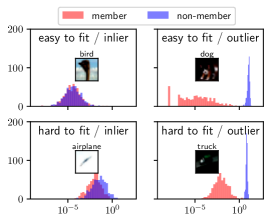
Figure 3: Some examples are easier to fit than others, and some have a larger separability between their losses when being a member of the training set or not. We train 1024 models on random subsets of CIFAR-10 and plot the losses for four examples when the example is a member of the training set ($\tilde{\mathbb{Q}}_{\text{in}}(x,y)$, in red) or not ($\tilde{\mathbb{Q}}_{\text{out}}(x,y)$, in blue).

Figure 3 plots histograms of model losses on four CIFAR-10 images when the image is contained in the model’s training dataset (red) and when it is absent (blue). We chose these images to illustrate two different axes of variation. On the columns we compare “inliers” to “outliers”, as determined by the model’s loss when not trained on the example. The left column shows examples with low loss when omitted from the training set, those in the right column have high loss. On rows we compare how easy the examples are to fit. The examples in the top row have very low loss when trained on, while the examples in the bottom row have higher loss. Importantly, observe that these two dimensions do measure different quantities. An example can be an outlier but easy to fit (upper right), or an inlier but hard to fit (lower left).

The goal of a membership inference adversary is to distinguish the two distributions in Figure 3 for a given example. This view illustrates the shortcomings of prior attacks (e.g., the LOSS attack): a global threshold on the observed loss $\ell(f(x),y)$ cannot distinguish between the different scenarios in Figure 3. The only confident assessment that such an attack can make is that examples with high loss are non-members. In contrast, the Likelihood-ratio test in Equation 2 considers the hardness of each example individually by modeling separate pairs of distributions $\tilde{\mathbb{Q}}_{\text{in}},\tilde{\mathbb{Q}}_{\text{out}}$ for each example $(x,y)$.

IV-C Estimating the likelihood-ratio with parametric modeling

We directly turn this observation into a membership inference attack by computing per-example hardness scores [56, 37, 68, 69]. By training models on random samples of data from the distribution $\mathbb{D}$, we obtain empirical estimates of the distributions $\tilde{\mathbb{Q}}_{\text{in}}$ and $\tilde{\mathbb{Q}}_{\text{out}}$ for any example $(x,y)$. And from here, we can estimate the likelihood from Equation 3 to predict if an example is a member of the training dataset or not.

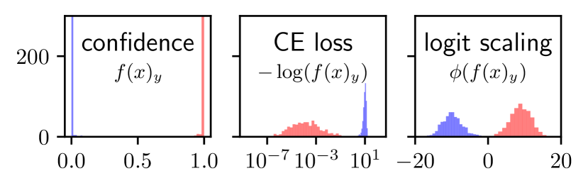
Figure 4: The model’s confidence, or its logarithm (the cross-entropy loss) are not normally distributed. Applying the logit function yields values that are approximately normal.

To improve performance at very low false-positive rates, instead of empirically modeling the distributions $\tilde{\mathbb{Q}}_{\text{in/out}}$ directly from the data, we opt for a parametric and model $\tilde{\mathbb{Q}}_{\text{in/out}}$ by Gaussian distributions. Parametric modeling has several significant benefits over nonparametric modeling.

• Parametric modeling requires training fewer shadow models to achieve the same generalization of nonparametric approaches. For example, we can match the recent (nonparametric) work of [69] with 400$\times$ fewer models.

• We can extend our attack to multivariate parametric models, allowing us to further improve attack success rate by querying the model multiple times (§VI-C).

Doing this requires some care. Indeed, as can be seen in Figure 3, the model’s cross-entropy loss is not well approximated by a normal distribution. First, the cross-entropy loss is on a logarithmic scale. If we take the negative exponent, $\exp(-\ell(f(x),y))$, we instead obtain the model “confidence” $f(x)_{y}$, which is bounded in the interval $[0,1]$ and thus not normally distributed either (i.e., the confidences for outliers and inliers concentrate, respectively, around $0$ and $1$). We thus apply a logit scaling to the model’s confidence,

$$\phi(p)=\log\left(\frac{p}{1-p}\right),\quad\text{ for }p=f(x)_{y}$$

to obtain a statistic in the range $(-\infty,\infty)$ that is (empirically) approximately normal. Figure 4 displays the distributions of model confidences, the negative log of the confidences (the cross-entropy loss), and the logit of the confidences. Only the logit appraoch is well approximated by a pair of Gaussians.

Our complete online attack (Algorithm 1). We first train $N$ shadow models [60] on random samples from the data distribution $\mathbb{D}$, so that half of these models are trained on the target point $(x,y)$, and half are not (we call these respectively IN and OUT models for $(x,y)$). We then fit two Gaussians to the confidences of the IN and OUT models on $(x,y)$ (in logit scale). Finally, we query the confidence of the target model $f$ on $(x,y)$ and output a parametric Likelihood-ratio test.

This attack is easily parallelized across multiple target points. Given a dataset $D\leftarrow\mathbb{D}$, we train shadow models on $N$ subsets of $D$, chosen so that each target $(x,y)\in D$ appears in $N/2$ subsets. The same $N$ shadow models can then be used to estimate the Likelihood-ratio test for all examples in $D$.

As an optimization, we can improve the attack by querying the target model on multiple points $x_{1},x_{2},\dots,x_{m}$ obtained by applying standard data augmentations to the target point $x$ (as previously observed in [6]). In this case, we fit $m$-dimensional spherical Gaussians $\mathcal{N}(\boldsymbol{\mu}_{\text{in}},\boldsymbol{\sigma}^{2}_{\text{in}}I),\mathcal{N}(\boldsymbol{\mu}_{\text{out}},\boldsymbol{\sigma}^{2}_{\text{out}}I)$ to the losses collected from querying the shadow models $m$ times per example, and compute a standard likelihood-ratio test between two multivariate normal distributions.

0:  model $f$, example $(x,y)$, data distribution $\mathbb{D}$

1:  $\text{confs}_{\text{in}}=\{\}$

2:  $\text{confs}_{\text{out}}=\{\}$

3:  for $N$ times do

4:     $D_{\text{attack}}\leftarrow^{\$}\mathbb{D}$ $\triangleright$ Sample a shadow dataset

5:     $f_{\text{in}}\leftarrow\mathcal{T}(D_{\text{attack}}\cup\{(x,y)\})$ $\triangleright$ train IN model

6:     $\text{confs}_{\text{in}}\leftarrow\text{confs}_{\text{in}}\cup\{\phi(f_{\text{in}}(x)_{y})\}$

7:     $f_{\text{out}}\leftarrow\mathcal{T}(D_{\text{attack}}{\setminus\{(x,y)\}})$ $\triangleright$ train OUT model

8:     $\text{confs}_{\text{out}}\leftarrow\text{confs}_{\text{out}}\cup\{\phi(f_{\text{out}}(x)_{y})\}$

9:  end for

10:  $\mu_{\text{in}}\leftarrow\texttt{mean}(\text{confs}_{\text{in}})$

11:  $\mu_{\text{out}}\leftarrow\texttt{mean}(\text{confs}_{\text{out}})$

12:  $\sigma_{\text{in}}^{2}\leftarrow\texttt{var}(\text{confs}_{\text{in}})$

13:  $\sigma_{\text{out}}^{2}\leftarrow\texttt{var}(\text{confs}_{\text{out}})$

14:  $\text{conf}_{\text{obs}}=\phi(f(x)_{y})$ $\triangleright$ query target model

15:  return  $\displaystyle\Lambda=\frac{p(\text{conf}_{\text{obs}}\ \mid\ \mathcal{N}(\mu_{\text{in}},\sigma^{2}_{\text{in}}))}{p(\text{conf}_{\text{obs}}\ \mid\ \mathcal{N}(\mu_{\text{out}},\sigma^{2}_{\text{out}}))}$

Algorithm 1 Our online Likelihood Ratio Attack (LiRA). We train shadow models on datasets with and without the target example, estimate mean and variance of the loss distributions, and compute a likelihood ratio test. (In our offline variant, we omit lines 5, 6, 10, and 12, and instead return the prediction by estimating a single-tailed distribution, as is shown in Equation 4.)

Our offline attack. While our online attack is effective, it has a significant usability limitation: it requires the adversary train new models after they are told to infer the membership of the example $(x,y)$. This requires training new machine learning models for every (batch of) membership inference queries, and is computationally expensive.

To improve the efficiency of our attack, we propose an offline attack algorithm that trains shadow models on randomly sampled datasets ahead of time, and never trains shadow models on the target points. For this attack, we remove lines 5,6,10 and 12 from Algorithm 1, and only estimate the mean $\mu_{\text{out}}$ and variance $\sigma_{\text{out}}^{2}$ of model confidences when the target example is not in the shadow models’ training data. We then change the likelihood-ratio test in line 15 to a one-sided hypothesis test. That is, we measure the probability of observing a confidence as high as the target model’s under the null-hypothesis that the target point $(x,y)$ is a non-member:

$$\Lambda=1-\Pr[Z>\phi(f(x)_{y})],\text{where }Z\sim\mathcal{N}(\mu_{\text{out}},\sigma^{2}_{\text{out}})\;.$$ (4)

The larger the target model’s confidence is compared to $\mu_{\text{out}}$, the higher the likelihood that the query sample is a member. Similar to our online attack, we improve the attack by querying on multiple augmentations and fitting a multivariate normal.

V Attack Evaluation

We now investigate our offline and online attack variants in a thorough evaluation across datasets and ML techniques.

Again, we focus extensively on the low-false positive rate regime. This is the setting with the most practical consequences: for example, to extract training data [4] it is far more important for attacks to have a low false positive rate than high average success, as false positives are fare more costly than false negatives. Similarly, de-identifying even a few users contained in a sensitive dataset is far more important than saying an average-case statement “most people are probably not contained in the sensitive dataset”.

We use both datasets traditionally used for membership inference attack evaluations, but also new datasets that are less typically used. In addition to the CIFAR-10 dataset introduced previously, we also consider three other datasets: CIFAR-100 [29] (another standard image classification task), ImageNet [9] (a standard challenging image classification task) and WikiText-103 [40] (a natural language processing text dataset). For CIFAR-100, we follow the same process as for CIFAR-10 and train a wide ResNet [71] to 60% accuracy on half of the dataset (25,000 examples). For ImageNet, we train a ResNet-50 on 50% of the dataset (roughly half a million examples). For WikiText-103, we use the GPT-2 tokenizer [53] to split the dataset into a million sentences and train a small GPT-2 [53] model on 50% of the dataset for 20 epochs to minimize the cross-entropy loss. Prior work has additionally performed experiments on two toy datasets that we do not believe are meaningful benchmarks for privacy because of their simplicity: Purchase and Texas (see [60] for details).

For each dataset, the adversary trains $N$ shadow models ($N=64$ for ImageNet, and $N=256$ otherwise) on training sets chosen so that each example $(x,y)$ is contained in exactly half of the shadow models’ training sets (thus, for each example we have $N/2$ IN models, and $N/2$ OUT models). We use the entire dataset for this purpose, and thus the training sets of individual shadow models and the target model may partially overlap. This is a strong assumption, which we make here mainly due to the small size of some of the datasets we consider. In Section VI-D, we show that our attack works just as well when the adversary trains shadow models on datasets that are fully disjoint from the target model’s training set.

For all datasets except ImageNet, we repeat each attack 10 times and report the attack success rates across all 10 attacks.

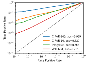
Figure 5: Success rate of our attack on CIFAR-10, CIFAR-100, ImageNet, and WikiText. All plots are generated with 256 shadow models, except ImageNet which uses 64.

V-A Online attack evaluation

Figure 5 presents the main results of our online attack when evaluated on the four more complex of the datasets mentioned above (CIFAR-10, CIFAR-100, ImageNet, and WikiText-103). Even though these datasets are complex, it is relatively efficient to train most of these models—for example a CIFAR-10 or CIFAR-100 model takes just six minutes to train. Additional results for the Purchase and Texas dataset are given in the Appendix—these datasets are much simpler and while they are typically used for membership inference, we argue they are too simple to have generalizable lessons.

Our attack has true-positive rates ranging from $0.1\%$ to $10\%$ at a false-positive rate of $0.001\%$. If we compare the three image datasets, consistent with prior works, we find that the attack’s average success rate (i.e., the AUC) is correlated directly with the generalization gap of the trained model. All three models have perfect $100\%$ training accuracy, but the test accuracy of the CIFAR-10 model is 90%, the ImageNet model is 65%, and the CIFAR-100 model is 60%. Yet, at low false-positives, the CIFAR-10 models are easier to attack than the ImageNet models, despite their better generalization.

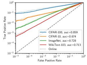
Figure 6: Success rate of our offline attack on CIFAR-10, CIFAR-100, ImageNet, and WikiText. All plots are generated with 128 OUT shadow models, except ImageNet which uses 32. For each dataset, we also plot our online attack with the same number of shadow models (half IN, half OUT).

	shadow models	multiple queries	class hardness	example hardness
					TPR @ 0.001% FPR			TPR @ 0.1% FPR			Balanced Accuracy
Method					C-10	C-100	WT103	C-10	C-100	WT103	C-10	C-100	WT103
Yeom et al. [70]	○	○	○	○	0.0%	0.0%	0.00%	0.0%	0.0%	0.1%	59.4%	78.0%	50.0%
Shokri et al. [60]	●	○	●	○	0.0%	0.0%	–	0.3%	1.6%	–	59.6%	74.5%	–
Jayaraman et al. [25]	○	●	○	○	0.0%	0.0%	–	0.0%	0.0%	–	59.4%	76.9%	–
Song and Mittal [61]	●	○	●	○	0.0%	0.0%	–	0.1%	1.4%	–	59.5%	77.3%	–
Sablayrolles et al. [56]	●	○	●	●	0.1%	0.8%	0.01%	1.7%	7.4%	1.0%	56.3%	69.1%	65.7%
Long et al. [37]	●	○	●	●	0.0%	0.0%	–	2.2%	4.7%	–	53.5%	54.5%	–
Watson et al. [68]	●	○	●	●	0.1%	0.9%	0.02%	1.3%	5.4%	1.1%	59.1%	70.1%	65.4%
Ye et al. [69]	●	○	●	●	-	-	-	-	-	-	60.3%	76.9%	65.5%
Ours	●	●	●	●	2.2%	11.2%	0.09%	8.4%	27.6%	1.4%	63.8%	82.6%	65.6%

TABLE I: Comparison of prior membership inference attacks under the same settings for well-generalizing models on CIFAR-10, CIFAR-100, and WikiText-103 using 256 shadow models. Accuracy is only presented for completeness; we do not believe this is a meaningful metric for evaluating membership inference attacks. Full ROC curves are presented in Appendix A.

V-B Offline attack evaluation

Figure 6 evaluates our offline attack from Section IV-C, where the adversary performs the costly operations of training shadow models only before being handed the target query point $(x,y)$. Our attack performs only slightly worse in this offline setting—at an FPR of $0.1\%$, our offline attack’s TPR is at most $20\%$ lower than that of our best online attack with the same number of shadow models.

V-C Re-evaluating prior membership inference attacks

In order to understand how our attack compares to prior work, we now re-evaluate prior attack techniques under our low-FPR objective. We study these attacks following the same evaluation protocol introduced above and on the same datasets (for WikiText, we omit a few entries for attacks that are not directly applicable to sequential language models).

A summary of our analysis is presented in Table I. We compare the efficacy of eight representative attacks from the literature. For each attack, we compute a full ROC curve and select a decision threshold that maximizes TPR at a given FPR. Surprisingly, we find that despite being published in 2019, the attack of Sablayrolles et al. [56] outperforms other attacks under our metric (often by an order of magnitude), even when compared to more recent attacks such as Jayaraman et al. [25] (PETS’21) and Song and Mittal [61] (USENIX’21).

Shadow models. One of the first membership inference attacks (due to Shokri et al. [60]) that improves on the baseline LOSS attack, introduced the idea of shadow models, but used in a simpler way than we have done here. Each shadow model $f_{i}$ (of a similar type to the target model $f$) is trained on random subsets $D_{i}$ of training data available to the adversary. The attack then trains a new neural network $g$ to predict an example’s membership status. Given the pre-softmax features $f_{i}(x)$ and class label $y$, the model $g$ predicts whether the data point $(x,y)$ was a member of the shadow training set $D_{i}$. For a target model $f$ and point $(x,y)$, the attack then outputs $g(f(x),y)$ as a membership confidence score.

We implement this by training shadow models that randomly subsample half of the total dataset. The training set of the shadow models thus partially overlaps with the training set of the target model $f$. This is a stronger assumption than that made by Shokri et al. [60] and thus yields a slightly stronger attack. Despite being significantly more expensive than the LOSS attack due to the overhead of training many shadow models and then training a membership inference predictor on the output of the models, this attack does not perform significantly better at low false-positive rates.

Multiple queries. It is possible to improve attacks by making multiple queries to the model. Jayaraman et al. [25] do this with their MERLIN attack, that queries the target model $f$ multiple times on a sample $x$ perturbed with fresh Gaussian noise, and measures how the model’s loss varies in the neighborhood of $x$. However, even when querying the target model $100$ times and carefully choosing the noise magnitude, we find that this attack does not improve the adversary’s success at low false-positive rates.

Choquette-Choo et al. [6] suggest an alternate technique to increase attack accuracy when models are trained with data augmentations. In addition to querying the model on $f(x)$, this attack also queries on augmentations of $x$ that the model might have seen during training. This is the direct motivation for us making these additional queries, which as we will show in Section VI-C improves our attack success rate considerably.

Per-class hardness. Instead of using per-example hardness scores as we have done, a potentially simpler method would be to design just one scoring function $\mathcal{A}^{\prime}_{y}$ per class $y$, by scaling the model’s loss by a class-dependent value: $\mathcal{A^{\prime}}_{y}(x,y)=\mathcal{A^{\prime}}(x,y)-\tau_{y}$. For example, in the ImageNet dataset [9] there are several hundred classes for various breeds of dogs, and so correctly classifying individual dog breeds tends to be harder than other broader classes. Interestingly, despite this intuition, in practice using per-class thresholds neither helps improve balanced attack accuracy nor attack success rates at low false-positive rates, although it does improve the AUC of attacks on CIFAR-10 and CIFAR-100 by $2\%$.

The attack of Song and Mittal [61] reported in Figure 1 and Table I combines per-class scores with additional techniques. Instead of working with the standard cross-entropy loss, this attack uses a modified entropy measure and trains shadow models to approximate the distributions of entropy values for members and non-members of each class. Given a model $f$ and target sample $(x,y)$, the attack computes a hypothesis test between the (per-class) member and non-member distributions (see [61]). Despite these additional techniques, this attack does not improve upon the baseline attack [60] at low FPRs.

Per-example hardness. As we do in our work, a final direction considers per-example hardness. Sablayrolles et al. [56] is the most direct influence for LiRA. Their attack, $\mathcal{A}^{\prime}(x,y)=\ell(f(x),y)-\tau_{x,y}$, scales the loss by a per-example hardness threshold $\tau_{x,y}$ that is estimated by training shadow models. Instead of fitting Gaussians to the shadow models’ outputs as we do, this paper takes a simpler non-parametric approach and sets the threshold near the midpoint $\tau_{x,y}=(\mu_{\text{in}}(x,y)+\mu_{\text{out}}(x,y))/2$ so as to maximize the attack accuracy; here $\mu_{\text{in}},\mu_{\text{out}}$ are the means computed as we do.

The recent work of Watson et al. [68] considers an offline variant of Sablayrolles et al. [56], that sets $\tau_{x,y}=\mu_{\text{out}}(x,y)$ (i.e., each example’s loss is calibrated by the average loss of shadow models not trained on this example).

Both Sablayrolles et al. and Watson et al. evaluate their attacks using average case metrics (balanced accuracy and AUC), and find that using per-example hardness thresholds can moderately improve upon past attacks. In our evaluation (Table I), we find that the balanced accuracy and AUC of their approaches are actually slightly lower than those of other simpler attacks. Yet, we find that per-example hardness-calibrated attacks reach a significantly better true-positive rate at low false-positive rates—and are thus much better attacks according to our suggested evaluation methodology.

The discrepancy between the balanced accuracy and our recommended low false-positive metric is even more stark for the attack of Long et al. [37]. This attack also trains shadow models to estimate per-example hardness, but additionally filters out a fraction of outliers to which the attack should be applied, and then makes no confident guesses for non-outliers. This attack thus cannot achieve a high average accuracy, yet outperforms most prior attacks at low false-positive rates.

To expand, this attack [37] builds a graph of all examples $x$, where an edge between $x$ and $x^{\prime}$ is weighted by the cosine similarity between the features $z(x)$ and $z(x^{\prime})$. Our implementation of this attack selects the $10\%$ of outliers with the largest distance to their nearest neighbor in this graph. For each such outlier $(x,y)$, the attack trains shadow models to numerically estimate the probability of observing a loss as high as $\ell(f(x),y)$ when $(x,y)$ is not a member.

The attack in the concurrent work of Ye et al. [69] is close in spirit to ours. They follow the same approach as our offline attack, by training multiple OUT models and then performing an exact one-sided hypothesis test. Specifically, to target an FPR of $\alpha$, their attack sets each example’s decision threshold so that an $\alpha$-fraction of the measured OUT losses for that example lie below the threshold.

The critical difference between our attack and these prior attacks is that we use a more efficient parametric approach, that models the distribution of losses as Gaussians. Since Sablayrolles et al. [56] and Watson et al. [68] only measure the means of the distributions, the attacks are sub-optimal if different samples’ loss distributions have very different scales and spreads (c.f. Figure 4). The attacks of Long et al. [37] and Ye et al. [69] take into account the full distribution of OUT losses, but have difficulties extrapolating to low FPRs due to the lack of a parametric assumption. By design, the exact test of Ye et al. [69] can at best target an FPR of $1/N$ with $N$ shadow models. It is thus inapplicable in the setting we consider here (256 shadow models, and a target FPR of $0.1\%$). Long et al. [37] extrapolate to the tails of the empirical loss distribution using cubic splines, which easily overfit and diverge outside of their support.

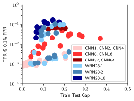
Figure 7: Attack true-positive rate versus model train-test gap for a variety of CIFAR-10 models.

V-D Membership inference and overfitting

To better understand the relationship between overfitting and vulnerability to membership inference attacks, Figure 7 plots various models’ train-test gap (that is, their train accuracy minus their test accuracy) versus our attack’s TPR at an FPR of $0.1\%$. We train CNN models and Wide ResNets (WRN) of various sizes on CIFAR-10, with different optimizers and data augmentations (see Section VI-E for details). Each point represents one training configuration for the target model.

While there is an overall trend that overfit models (those with higher train-test gap) are more vulnerable to attack, we do find examples of models that have identical train-test gaps but are $\textbf{100}\times$ more vulnerable to attack. In Figure 16 in the Appendix we further plot the attack TPR as a function of the test accuracy of these models. There, we observe a clear trend that more accurate models are more vulnerable to attack.

Attack Approach	TPR @ 0.1% FPR
LOSS attack [70]	0.0%
+ Logit scaling	0.1%
+ Multiple queries	0.1%
LOSS attack [70]	0.0%
+ Per-example thresholds ($\tilde{\mathbb{Q}}_{\text{out}}$ only) [68]	1.3%
+ Logit scaling	4.7%
+ Gaussian Likelihood	4.7%
+ Multiple queries (our offline attack)	7.1%
LOSS attack [70]	0.0%
+ Per-example thresholds ($\tilde{\mathbb{Q}}_{\text{in}}$ & $\tilde{\mathbb{Q}}_{\text{out}}$) [56]	1.7%
+ Logit scaling	1.9%
+ Gaussian Likelihood	5.6%
+ Multiple queries (our online attack)	8.4%

TABLE II: By iteratively adding the main components of our attack we can interpolate between the simple LOSS threshold attack [70] and our full offline and online attacks.

VI Ablation Study

Our attack has a number of moving pieces that are connected in various ways; in this section we investigate how these pieces come together to reach such high accuracy at low false-positive rates. We exclusively use CIFAR-10 for these ablation studies as it is the most popular image classification dataset and is the hardest datasets we have considered;

A summary of our analysis is presented in Table II. The baseline LOSS attack achieves a true-positive rate of $0\%$ at a false positive rate of $0.1\%$ (as shown previously in Figure 2(b)). If we do not use per-example thresholds, this basic attack can only be marginally improved by properly scaling the loss and issuing multiple queries to the target model.

By incorporating per-example thresholds obtained by estimating the distributions $\tilde{\mathbb{Q}}_{\text{in}}$ and $\tilde{\mathbb{Q}}_{\text{out}}$ as in [56], the attack success rate increases to $1.7\%$—about one-order-of-magnitude better than chance. By ensuring that we appropriately re-scale the model losses (explored in detail in Section VI-A) and fitting the re-scaled losses with Gaussians (see Section VI-B), we increase the attack success rate by a factor of $3.3\times$. Finally, we can nearly double the attack success rate by evaluating the target model on the same data augmentations as used during training, as we will show in Section VI-C.

We also perform the same ablation but with the offline variant of our attack. Here, if we start with the attack of Watson et al. [68] to reach a $1.3\%$ true-positive rate; adding logit scaling, Gaussian likelihood, and multiple queries yields an attack that is nearly as strong as our full attack (TPR of $7.1\%$ versus $8.4\%$ at an FPR of $0.1\%$).

VI-A Logit scaling the loss function

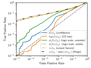
Figure 8: The best scoring metrics ensure the output distribution is approximately Gaussian, and the worst metrics are not easily modeled with a standard distribution (see Figure 4).

The first step of our attack projects the model’s confidences to a logit scale to ensure that the distributions that we work with are approximately normal. Figure 8 compares performance of our attack for various choices of statistics that we can fit using shadow models. Recall that we defined our neural network function $f(x)$ to denote the evaluation of the model along with a final softmax activation function; we use $z(x)$ to denote the pre-softmax activations of the neural network.

As expected, we find that using the model’s confidence $f(x)_{y}\in[0,1]$, or its logarithm (the cross-entropy loss), leads to poor performance of the attack since these statistics do not behave like Gaussians (recall from Figure 4).

Our logit rescaling performs best, but the exact numerical computation of the logit function $\phi(p)=\log(\frac{p}{1-p})$ matters. We consider two mathematically equivalent variants:

$$\phi_{\text{unstable}} =\log(f(x)_{y})-\log(1-f(x)_{y})$$

$$\phi_{\text{stable}} =\log(f(x)_{y})-\log\sum_{y^{\prime}\neq y}f(x)_{y^{\prime}}\;.$$

We find that the second version is more stable in practice, when the model’s confidence is very high, $f(x)_{y}\approx 1$ (we compute all logarithms as $\log(x+\epsilon)$ for a small $\epsilon>0$). Note that this second stable variant requires access to the full vector of model confidences $f(x)\in[0,1]^{n}$ rather than just the confidence of the predicted class.

If the adversary can query the model to obtain the unnormalized features $z(x)$ (i.e., the outputs of the model’s last layer before the softmax function), a hinge loss performs similarly

$$\ell_{\text{Hinge}}(x,y)=z(x)_{y}-\max_{y^{\prime}\neq y}z(x)_{y^{\prime}}\;.$$

To see why this is the case, observe that

$$\phi(f(x)_{y}) =\log(f(x)_{y})-\log\sum_{y^{\prime}\neq y}f(x)_{y^{\prime}}$$

$$=z(x)_{y}-\underset{y^{\prime}\neq y}{\operatorname{LogSumExp}}\ z(x)_{y^{\prime}}\;,$$

where the $\operatorname{LogSumExp}$ function is a smooth approximation to the maximum function. When the features $z(x)$ are available, we recommend using the hinge loss as its computation is numerically simpler than that of the logit-scaled confidence.

We note that the different attack variants we consider here lead to orders-of-magnitude differences in attack performance at low false-positive rates—even though all variants achieve similar AUC scores (68–72%). This again highlights the importance of carefully designing attacks, and of measuring attack performance at low false-positive rates rather than on average across the entire ROC curve.

The choice of an appropriate loss function can also have a major impact on previous MIAs. For example, for the attack of Watson et al. [68] (which scales the model’s loss by the mean loss of OUT models not trained on the example, $\mu_{\text{out}}(x,y)$) applying logit scaling nearly quadruples the attack’s true-positive rate at an FPR of 0.1% (see Table II).

VI-B Gaussian distribution fitting

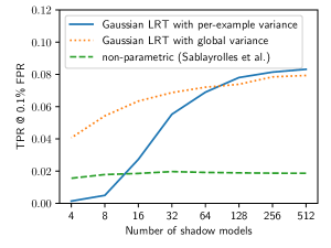
Figure 9: Attack success rate increases as the number of shadow models increases, with the benefit eventually tapering off. When fewer than 64 models are used, it is better to estimate the variance of the model confidence as a global parameter instead of computing it on a per-example basis.

Like other shadow models membership inference attacks [60], our attack requires that we train enough models to accurately estimate the distribution of losses. It is thus desirable to minimize the number of shadow models that are necessary. However, most prior works in Table I that rely on shadow models do not analyze this tradeoff and report results only for a fixed number of shadow models [60, 37, 56].

Figure 9 displays our online attack’s TPR at a fixed FPR of 0.1%, as we vary the number of shadow models (half IN and half OUT). Training more than $64$ shadow models provides diminishing benefits, but the attack deteriorates quickly with fewer models—due to the difficulty of fitting Gaussian distributions on a small number of data points.

With a small number of shadow models, we can improve the attack considerably by estimating the variances $\sigma_{\text{in}}^{2}$ and $\sigma_{\text{out}}^{2}$ of model confidences in Algorithm 1 globally rather than for each individual example. That is, we still estimate the means $\mu_{\text{in}}$ and $\mu_{\text{out}}$ separately for each example, but we estimate the variance $\sigma_{\text{in}}^{2}$ (respectively $\sigma_{\text{out}}^{2}$) over the shadow models’ confidences on all training set members (respectively non-members).

For a small number of shadow models ($<64$), estimating a global variance outperforms our general attack that estimates the variance for each example separately. For a larger number of models, our full attack is stronger: with $1024$ shadow models for example, the TPR decreases from $8.4\%$ to $7.9\%$ by using a global variance.

VI-C Number of queries

Models are typically trained to minimize their loss not only on the original training example, but also on augmented versions of the example. It therefore makes sense to perform membership inference attacks on the augmented versions of the example that may have been seen during training. Results of this analysis are presented in Table III. There are $162$ potential augmentations of each training image for our CIFAR-10 model ($2\times 9\times 9$, computed by either horizontally flipping the image or not, and shifting the image by up to $\pm 4$ pixels in each height or width). We find that querying on just $2$ augmentations gives most of the benefit, with increasing to 18 queries performing identically to all $162$ augmentations.

	TPR @ FPR
Queries	0.1%	0.001%
1 (no augmentations)	5.6%	1.0%
2 (mirror)	7.5%	1.8%
18 (mirror + shifts)	8.4%	2.2%
162 (mirror + shifts)	8.4%	2.2%

TABLE III: Querying on augmented versions of the image doubles the true-positive rate at low false-positive rates, with most benefits given by just two queries.

VI-D Disjoint datasets

In our experiments so far, we trained both the target models and the adversary’s shadow models by subsampling from a common dataset. That is, we use a large dataset $D_{\text{attack}}$ (e.g., the entire CIFAR-10 dataset) to train shadow models, and the target model’s training set $D_{\text{train}}$ is some (unknown) subset of this dataset. This setup favors the attacker, as the training sets of shadow models and the target model can partially overlap.

In a real attack, the adversary likely has access to a dataset $D_{\text{attack}}$ that is disjoint from the training set $D_{\text{train}}$. We now show that this more realistic setup has only a minor influence on the attack’s success rate.

For this experiment, we use the CINIC-10 dataset [8]. This dataset combines CIFAR-10 with an additional 210k images taken from ImageNet that correspond to classes contained in CIFAR-10 (e.g., bird/airplane/truck etc). We train a target model and 128 shadow models (OUT models only) each on 50,000 points. We compare three attack setups:

1. The shadow models’ training sets are sampled from the full CINIC-10 dataset. This is the same setup as in all our previous experiments, where $D_{\text{train}}\subset D_{\text{attack}}$.

2. The shadow models’ training sets have no overlap with the target model, i.e., $D_{\text{train}}\cap D_{\text{attack}}=\emptyset$.

3. The target model is trained on CIFAR-10, while the attacker trains shadow models on the ImageNet portion of CINIC-10. There is thus a distribution shift between the target model’s dataset and the attacker’s dataset.

Figure 10 shows that our attack’s performance is not influenced by an overlap between the training sets of the target model and shadow models. The attack success is unchanged when the attacker uses a disjoint dataset. A distribution shift between the training sets of the target model and shadow models does reduce the attack’s TPR. Surprisingly, the attack’s AUC is much higher when there is a distribution shift—we leave an explanation of this phenomenon to future work.

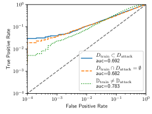
Figure 10: The attack’s success rate on CINIC-10 remains unchanged when the training sets of shadow models are sampled from a dataset $D_{\text{attack}}$ that is disjoint from the target model’s training set $D_{\text{train}}$. The attack’s performance does decrease when the two datasets are sampled from different distributions.

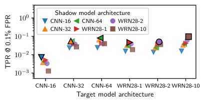
(a) Vary model architecture.

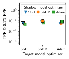
(b) Vary training optimizer.

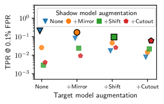
(c) Vary data augmentation.

Figure 11: Our attack succeeds when the adversary is uncertain of the target model’s training setup. We vary the target model’s architecture (a), the training optimizer (b) and the data augmentation (c), as well as the adversary’s guess of each of these properties when training shadow models. The attack performs best when the adversary guesses correctly (black-lined markers).

VI-E Mismatched training procedures

We now explore how our attack is affected if the attacker does not know the exact training procedure of the target model. We train models with various architectures, optimizers, and data augmentations to investigate the attack’s performance when the adversary guesses each of these incorrectly. For each attack, we train $64$ shadow models and use our online attack variant with a global estimate of the variance (see Section VI-B). Figure 11 summarizes our results at a fixed FPR of $0.1\%$. Appendix Figures 22, 23 and 24 have full ROC curves.

In Figure 11(a), we vary the target model’s architecture. We study three CNN models (with 16, 32 and 64 convolutional filters), and three Wide ResNets (WRN) with width 1, 2 and 10. All models are trained with SGD with momentum and with random augmentations. Our attack performs best when the attacker trains shadow models of the same architecture as the target model, but using a similar model (e.g., a WRN28-1 instead of a WRN28-2) has a minimal effect on the attack. Moreover, we find that for both the CNN and WRN model families, larger models are more vulnerable to attacks.

In Figure 11(b) we fix the architecture to a WRN28-10, and vary the training optimizer: SGD, SGDM (SGD with momentum) or Adam. For both the defender or the attacker, the choice of optimizer has minimal impact on the attack.

Finally, in Figure 11(c) we fix the architecture (WRN28-10) and optimizer (SGDM) and vary the data augmentation used for training: none, mirroring, mirroring + shifts, mirroring + shifts + cutout. The attacker’s guess of the data augmentation is used both to train shadow models, and to create additional queries for the attack. We find that correctly guessing the target model’s data augmentation has the highest impact on attack performance. Models trained with stronger augmentations are harder to attack, as these models are less overfit.

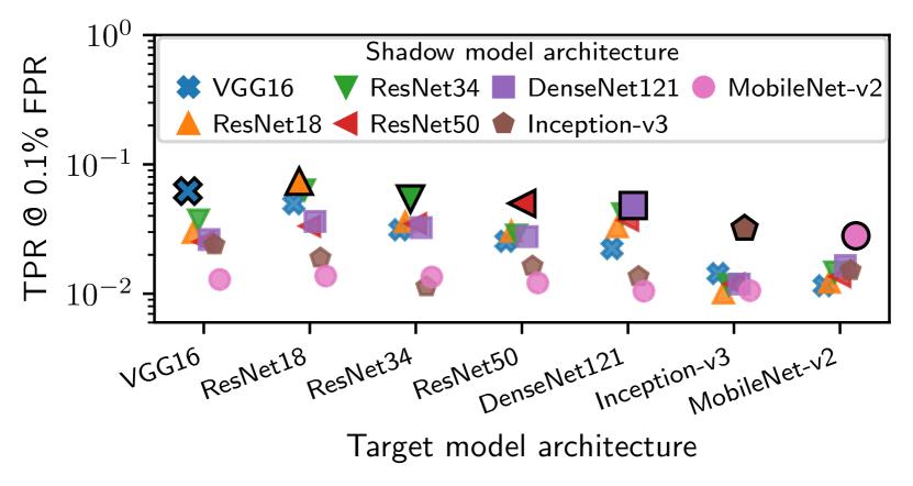
Figure 12: Our attack succeeds against real state-of-the-art CIFAR-10 models [51]. The attacker trains shadow models on a random subset of $50{,}000$ points from the entire CIFAR-10 dataset. The attack performs best when the shadow models have the same architecture as the target model, but training different models still leads to a strong attack.

VII Additional Investigations

We now pivot from evaluating our attack to using our attack as a tool to better understand memorization in real models (§VII-A) and why memorization occurs (§VII-B).

VII-A Attacking real-world models

All our experiments so far have involved attacking models that we ourselves have trained. To ensure that we did not somehow train weakly accidentally private (or non-private) models, we now show that our attacks also succeed on existing pre-trained state-of-the-art models. To this end, we load standard models pre-trained by Phan [51] on the complete CIFAR-10 training set (50,000 examples). We train 256 shadow models by using the same training code and subsampling $50{,}000$ points at random from the entire CIFAR-10 dataset ($60{,}000$ examples). On average, we have $213$ IN models and $43$ OUT models per example. Figure 12 shows our attack’s true-positive rate at a 0.1% FPR for various canonical model architectures.

We consider two attack variants: (1) the adversary knows the target model’s architecture and uses it to train the shadow models; (2) the shadow models use a different architecture than the target model. Since we only have $43$ models to estimate the distribution $\tilde{\mathbb{Q}}_{\text{out}}$), esitmating a global variance for all examples performs best. The results of this experiment are qualitatively similar to those in Section VI-E: (1) the model architecture has a small effect on the privacy leakage (e.g., the attack works better against a ResNet-18 than against a MobileNet-v2); (2) the attack works best when the shadow models share the same architecture as the target model, but it is robust to architecture mismatches. For example, attacking a ResNet-34 model with either ResNet-18 or ResNet-50 shadow models leads to a minor drop in attack success rate (from 5% TPR to 4% TPR).

Figure 13: Out-of-distribution training examples are less private.

VII-B Why are some examples less private?

While our average attack success rate is modest, the success rate at low false-positive rates can be very high. This suggests that there is a subset of examples that are easier to attack than others. While a full investigation of this is beyond the scope of our paper, we find an important factor behind why some samples are less private is that they are out-of-distribution.

To make this argument, we intentionally inject out-of-distribution examples into a model’s training dataset and compare the difficulty of attacking these newly inserted samples versus typical examples. Specifically, we insert $1{,}000$ examples from various out-of-distribution sources into the $50{,}000$-example CIFAR-10 training dataset to form a new augmented $51{,}000$ example dataset. We then train shadow models on this dataset, run our attack, and measure the distinguishability of distributions of losses for IN and OUT models for each of the $1{,}000$ newly inserted examples (we use a simple measure of distance between distributions here, defined as $d=\frac{|\mu_{\text{in}}-\mu_{\text{out}}|}{\sigma_{\text{in}}+\sigma_{\text{out}}}$). Figure 13 plots the distribution of these “privacy scores” assigned to each example. As a baseline, in blue, we show the distribution of privacy scores for the standard CIFAR-10 dataset; these are tightly concentrated around 0.

Next we show the privacy scores of examples inserted from the CINIC-10 dataset, which are drawn from ImageNet. Due to this slight distribution shift, the CINIC-10 images have a larger privacy score on average: it is easier to detect their presence in the dataset because they are slightly out-of-distribution.

We can extend this further by inserting intentionally mislabeled images that are extremely out-of-distribution. If we choose $1{,}000$ images (shown in red) from the CIFAR-10 test set and assign new random labels to each image, then we get a much higher privacy score for these images. Finally, we interpolate between the extreme OOD setting of random (and thus incorrectly) labeled CIFAR-10 images and correctly-labeled CINIC-10 by inserting randomly labeled images from CIFAR-100 (shown in green). Because these images come from a disjoint class distribution, models will not typically be confident on their label one way or another unless they are seen during training. The privacy scores here fall in between correctly labeled CINIC-10 and incorrectly labeled CIFAR-10.

VIII Conclusion

As we have argued throughout this paper, membership inference attacks should focus on the problem of achieving high true-positive rates at low false-positive rates. Our attack presents one way to succeed at this goal. There are a number of different evaluation directions that we hope future work will explore under this direction.

Membership inference attacks as a privacy metric. Both researchers [42] and practitioners [63] use membership inference attacks to measure privacy of trained models. We argue that these metrics should use strong attacks (such as ours) in order to accurately measure privacy leakage. Future work using membership inference attacks should consider the low false-positive rate regime, to better understand if the privacy of even just a few users can be confidently breached.

Usability improvements to membership inference attacks. The key limitation of per-example membership inference attacks is that they require new hyperparameters that need to be learned from the data. While it is much more important that attacks are strong (even if slow) as opposed to fast (but weak), we hope that future work will improve the computational efficiency of our attack approach, in order to allow it to be deployed in more settings.

Improving other privacy attacks with our method. Membership inference attacks form the basis for many other privacy attack methods [17, 3, 4]. Our membership inference method, in principle, should be able to directly improve these attacks.

Rethinking our current understanding of MIA results. The literature on membership inference attacks has answered a number of memorization questions. However, many (or even most) of these prior papers focused on the inadequate metric of average-case attack success rates, instead of on the low false-positive rate regime. As a result it will be necessary to re-investigate prior results from this perspective:

• Do previously-“broken” [45, 26] defenses prevent our attack? Prior defenses were only ever shown to be ineffective at preventing an adversary from succeeding on average—not confidently at low false-positive rates.

• How does differential privacy interact with our improved attacks? We have preliminary evidence that vacuous guarantees might prevent our low-FPR attacks (Section A-A).

• Are attacks with reduced capabilities possible? For example, label-only attacks [6, 54, 34] can match the balanced accuracy of shadow-model approaches. But do these attacks work at low false-positive rates?

• Are attacks with extra capabilities more effective? Prior work has shown that access to gradient queries [46] or intermediate models [58] improves attack AUC. However, does this observation hold at low false-positive rates?

We hope that future work will be able to answer these questions, among many more, in order to better evaluate (and develop) techniques that preserve the privacy of training data. By developing attacks that succeed low false-positive rates, we can evaluate privacy not as a measurement of the average user, but of the most vulnerable.

Appendix A Additional Experiments

A-A Attacking DP-SGD

Machine learning with differential privacy [1] is the main defence mechanism against privacy attacks including membership inference against machine learning models. Differential privacy provides an upper bound on the success of any membership inference attack. Recent works [47, 24] thus used membership attacks to empirically audit differential privacy bounds, in particular those obtained from DP-SGD [1]. In this work, we are interested in the effect of DP-SGD on the performance of our membership inference attack.

We consider different combinations of DP-SGD’s noise multiplier and clipping norm parameters in our evaluation. Table IV summarizes the average accuracy of standard CNN models trained on CIFAR-10 with DP-SGD for different parameter sets. We evaluate the effectiveness of our membership inference attacks for these settings in Figure 14. Even just clipping the gradient norm without adding any noise reduces the performance of our attack significantly. However, small clipping norms can reduce the accuracy of the models as shown in Table IV.

TABLE IV: Accuracy of the models trained with DP-SGD on CIFAR10 with different noise parameters

Noise Multiplier ($\sigma$)	$C=10$	$C=5$	$C=1$
0.0	84.0%	78.5%	61.3%
0.2	73.9%	77.1%	62.8%
0.8	36.9%	43.3%	61.3%

For higher clipping norms, adding very small amounts of noise (Figure 14-b) reduces the effectiveness of the membership inference attack to chance, while resulting in models with higher accuracy.

Training models with very small amounts of noise is an effective defense against our membership inference attack, despite resulting in very large provable DP bounds $\epsilon$.

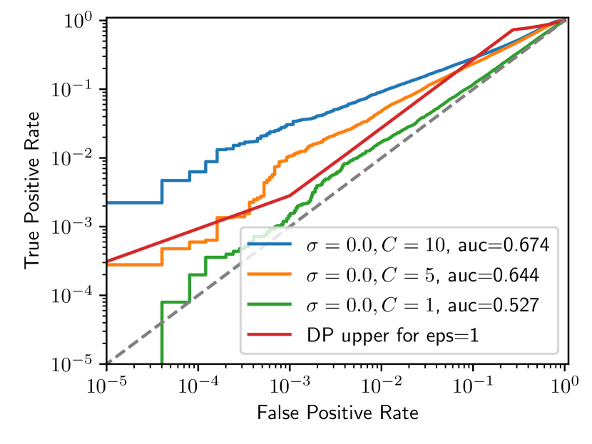
(a) $\epsilon=\infty$

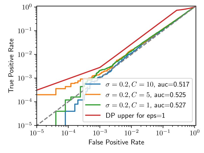
(b) $\epsilon>5000$

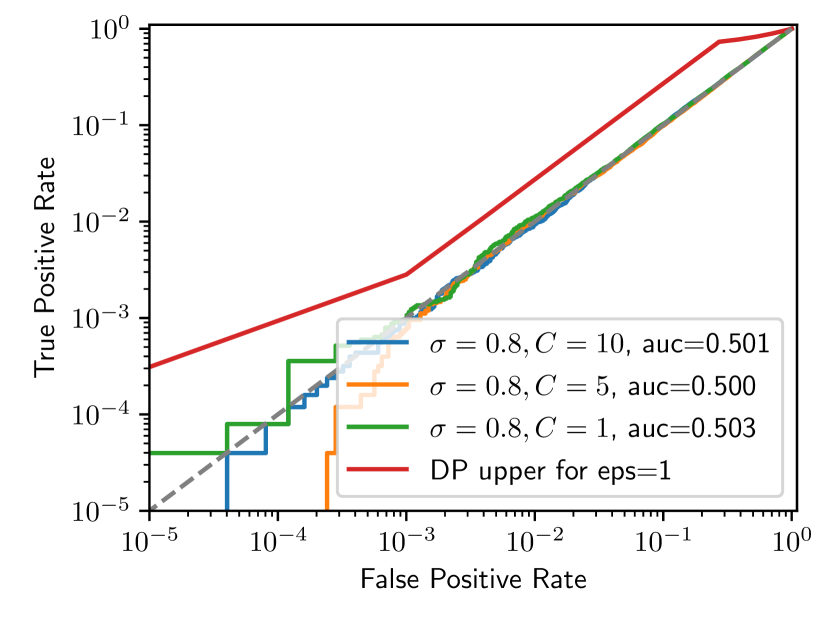
(c) $\epsilon=8$

Figure 14: Effectiveness of using DP-SGD against our attack with different privacy budgets.

A-B White-box Attacks

Previous works [46, 62] suggested that is possible to achieve better membership inference if the adversary has white-box access to the target model. In particular, previous works showed that using the norm of the model’s gradient at a target point could increase the balanced accuracy of membership inference attacks. Figure 15 highlights the comparison between a white-box and a black-box adversary. The results show that using gradient norms will improve the overall AUC both for our online attack, as well as when using a global threshold as in the LOSS attack. However, at lower false-positive rates we do not observe any improvement of using gradient norms compared to just using model confidences.

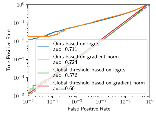
Figure 15: Comparison of the white-box attack using our approach to the black-box setting.

Appendix B Additional Figures and Tables

B-A Attack Performance versus Model Accuracy

In Section V-D, Figure 7 we plotted the relationship between a model’s train-test gap and its vulnerability to membership inference attacks. In Figure 16, we look at the attack success rate as a function of the test accuracy of the same models. There is a clear trend where better models are more vulnerable to attacks. Prior work reported a similar phenomenon for data extraction attacks [3, 4].

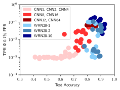
Figure 16: Attack true-positive rate versus model test accuracy.

B-B Full ROC Curves for Gaussian Distribution Fitting

In Figure 17, we show full (log-scale) ROC curves for the experiment in Section VI-B, where we explored the effect of varying the number of shadow models on the success rate of our online attack. We vary the number of shadow models from $4$ to $256$ and consider two attack variants: (1) fit Gaussians for each example by estimating the means $\mu_{\text{in}},\mu_{\text{out}}$ and variances $\sigma_{\text{in}}^{2},\sigma_{\text{out}}^{2}$ independently for each example; (2) estimate the means $\mu_{\text{in}},\mu_{\text{out}}$ for each example, but estimate global variances $\sigma_{\text{in}}^{2},\sigma_{\text{out}}^{2}$. As we observed in Section VI-B, estimating per-example variances works poorly when the number of shadow models is small ($<64$). With a global estimate of the variance, the attack performs nearly on par with our best attack with as little as 16 shadow models.

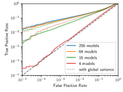
Figure 17: Effect of varying the number of models trained on attack success rates. It is always useful to estimate the mean per-example difficulty; however when only a few models are available, it is orders of magnitude more effective to assign all examples the same variance.

B-C Comparison to Prior Work on Additional Datasets

Similarly to Figure 1 for CIFAR-10, we compare our attack against prior membership inference attacks on additional datasets: CIFAR-100 in Figure 18, WikiText-103 in Figure 19, Texas in Figure 21 and Purchase in Figure 21.

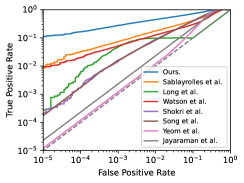
Figure 18: ROC curve of prior membership inference attacks, compared to our attack, on CIFAR-100.

Figure 19: ROC curve of prior membership inference attacks, compared to our attack, on WikiText-103. We omit prior attacks that rely on the model features $z(x)$, as these attacks were not designed for sequential models.

dummy text so that figures are nicely top-aligned

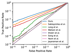
Figure 20: ROC curve of prior membership inference attacks, compared to our attack, on the Texas dataset.

Figure 21: ROC curve of prior membership inference attacks, compared to our attack, on the Purchase dataset.

dummy text so that figures are nicely top-aligned

B-D Attack Ablations on Additional Datasets

Similarly to Table II for CIFAR-10, we now perform ablations on the different components of our attack for CIFAR-100 (Table V), WikiText-103 (Table VI), Texas (Table VII) and Purchase (Table VIII). Note that for WikiText-103, Texas and Purchase, we train models without any data augmentations and thus do not perform augmentations in the attack either.

As we observed in Section VI for CIFAR-10, a Gaussian Likelihood Test after logit scaling significantly boosts the performance of past attacks that rely on per-example thresholds, both in the offline case and in the online case.

In contrast to CIFAR-10, we observe that logit scaling on its own is often detrimental to the online attack of Sablayrolles et al. [56]. Similarly, we find that a Gaussian Likelihood Test on its own (i.e., without logit scaling) often hurts the attack performance. Thus, these two components necessarily have to be applied together to achieve a good attack performance.

Attack Approach	TPR @ 0.1% FPR
LOSS attack [70]	0.0%
+ Logit scaling	0.1%
+ Multiple queries	0.1%
LOSS attack [70]	0.0%
+ Per-example thresholds ($\tilde{\mathbb{Q}}_{\text{out}}$ only) [68]	5.2%
+ Logit scaling	14.7%
+ Gaussian Likelihood	18.9%
+ Multiple queries (our offline attack)	22.3%
LOSS attack [70]	0.0%
+ Per-example thresholds ($\mathbb{Q}_{\text{in}}$ & $\mathbb{Q}_{\text{out}}$) [56]	7.4%
+ Logit scaling	2.8%
+ Gaussian Likelihood	24.1%
+ Multiple queries (our attack)	27.6%

TABLE V: Breakdown of how various components build up to obtain our best attacks on the CIFAR-100 dataset.

Attack Approach	TPR @ 0.1% FPR
LOSS attack [70]	0.1%
+ Logit scaling	0.1%
LOSS attack [70]	0.1%
+ Per-example thresholds ($\tilde{\mathbb{Q}}_{\text{out}}$ only) [68]	1.1%
+ Logit scaling	1.1%
+ Gaussian Likelihood (our offline attack)	1.2%
LOSS attack [70]	0.1%
+ Per-example thresholds ($\mathbb{Q}_{\text{in}}$ & $\mathbb{Q}_{\text{out}}$) [56]	1.0%
+ Logit scaling	1.0%
+ Gaussian Likelihood (our attack)	1.4%

TABLE VI: Breakdown of how various components build up to obtain our best attacks on the WikiText-103 dataset.

B-E Full ROC Curves for Mismatched Training Procedures

In Figures 22, 23 and 24, we plot full ROC curves for the experiments from Section VI-E, where the attacker has to guess the architecture, optimizer and data augmentation used by the target model.

Attack Approach	TPR @ 0.1% FPR
LOSS attack [70]	0.1%
+ Logit scaling	0.1%
LOSS attack [70]	0.1%
+ Per-example thresholds ($\tilde{\mathbb{Q}}_{\text{out}}$ only) [68]	8.8%
+ Logit scaling	19.0%
+ Gaussian Likelihood (our offline attack)	24.6%
LOSS attack [70]	0.1%
+ Per-example thresholds ($\mathbb{Q}_{\text{in}}$ & $\mathbb{Q}_{\text{out}}$) [56]	14.9%
+ Logit scaling	8.4%
+ Gaussian Likelihood (our attack)	33.2%

TABLE VII: Breakdown of how various components build up to obtain our best attacks on the Texas dataset.

Attack Approach	TPR @ 0.1% FPR
LOSS attack [70]	0.0%
+ Logit scaling	0.1%
LOSS attack [70]	0.0%
+ Per-example thresholds ($\tilde{\mathbb{Q}}_{\text{out}}$ only) [68]	1.5%
+ Logit scaling	1.3%
+ Gaussian Likelihood (our offline attack)	1.4%
LOSS attack [70]	0.0%
+ Per-example thresholds ($\mathbb{Q}_{\text{in}}$ & $\mathbb{Q}_{\text{out}}$) [56]	2.7%
+ Logit scaling	0.2%
+ Gaussian Likelihood (our attack)	4.1%

TABLE VIII: Breakdown of how various components build up to obtain our best attacks on the Purchase dataset.

dummy text so that tables are nicely top-aligned

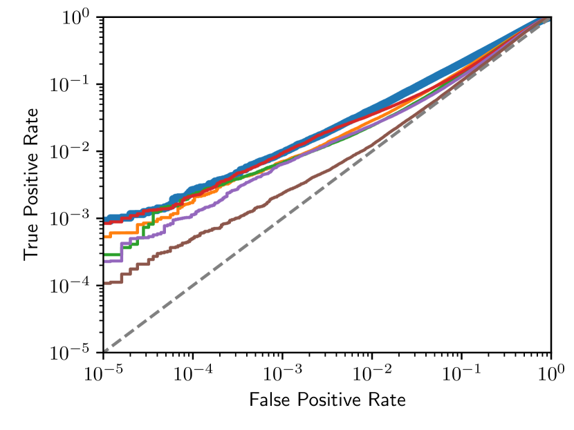
(a) CNN-16 as target.

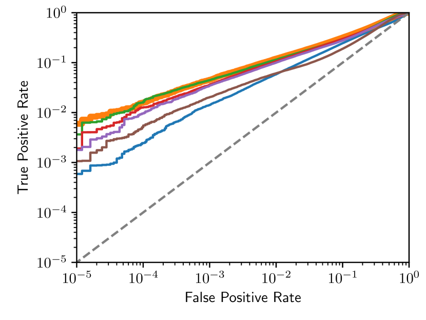
(b) CNN-32 as target.

(c) CNN-64 as target.

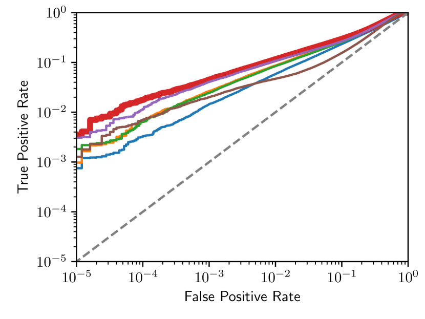
(d) WRN28-1 as target.

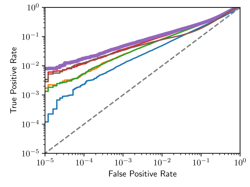
(e) WRN28-2 as target.

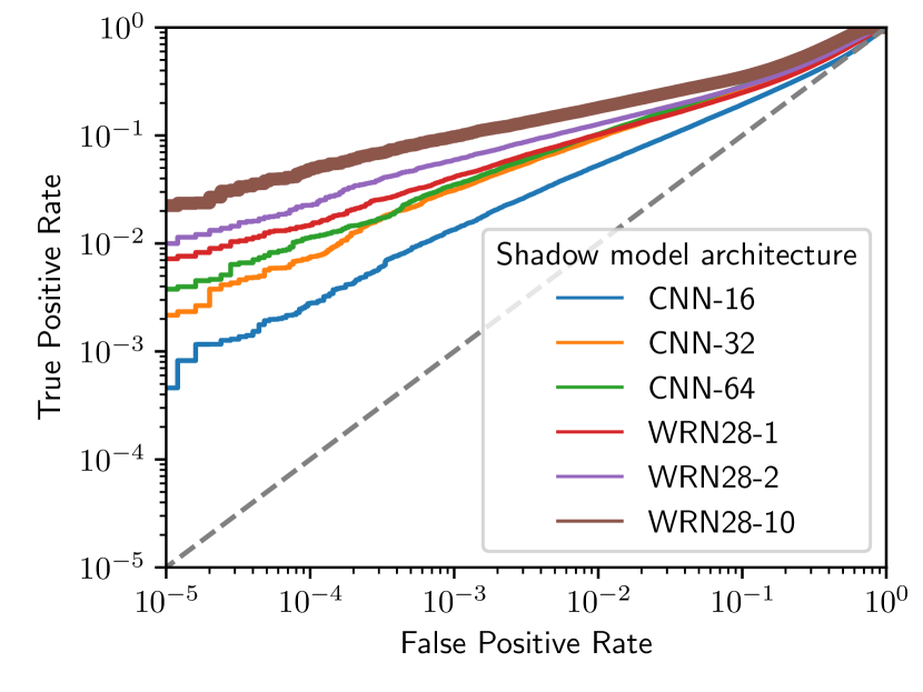
(f) WRN28-10 as target.

Figure 22: Different architectures with momentum optimizer and mirror & shift as augmentation.

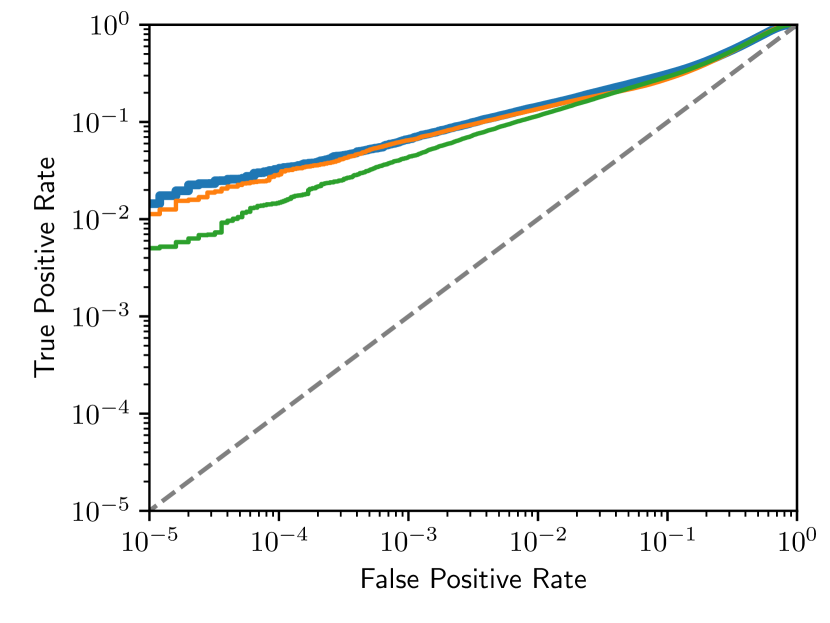
(a) SGD as target.

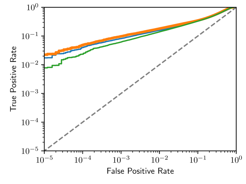
(b) Momentum as target.

(c) Adam as target.

Figure 23: Different optimizers on WRN28-10 with mirror & shift as augmentation.

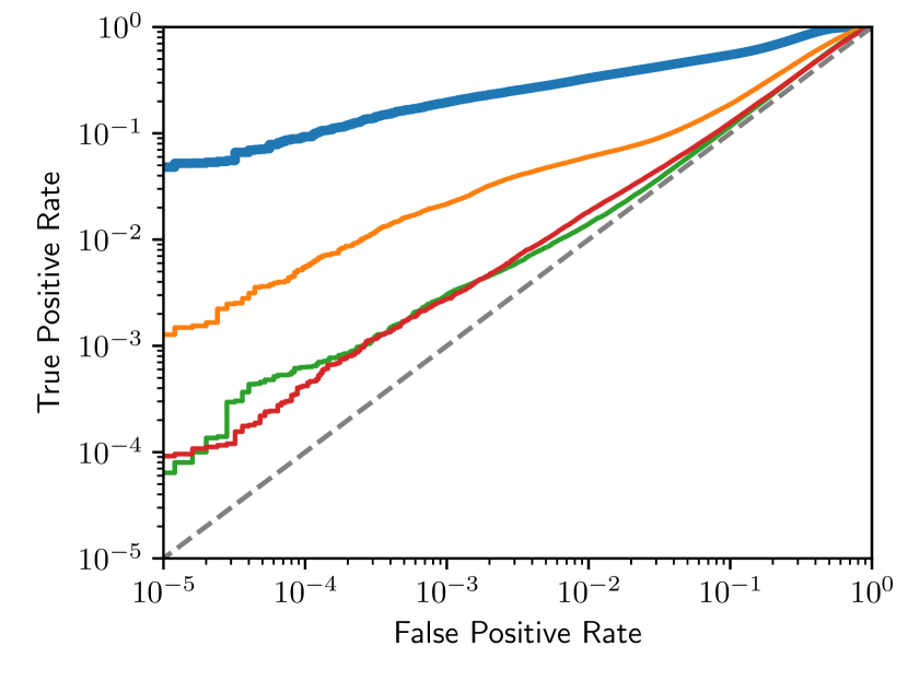
(a) No augmentation.

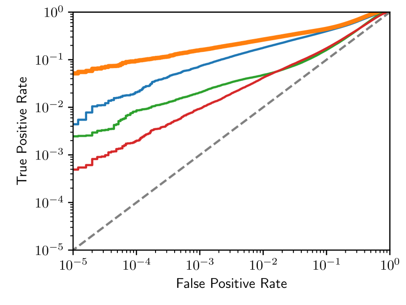
(b) Mirror.

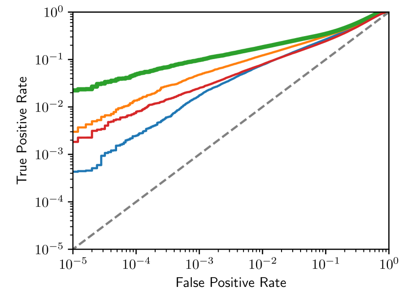
(c) Mirror+Shift.

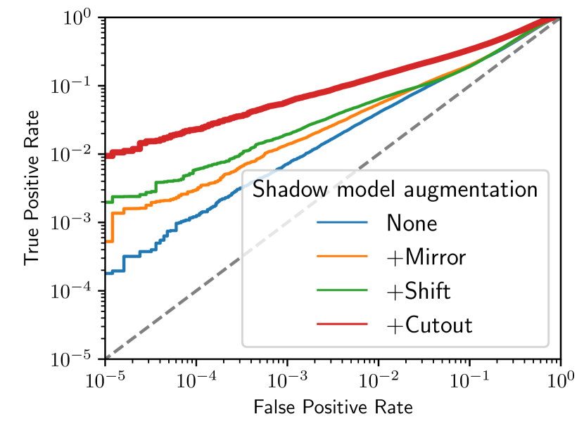
(d) Mirror+Shift+Cutout16.

Figure 24: Different augmentations on WRN28-10 with momentum optimizer.

References

- Abadi et al. [2016] Martin Abadi, Andy Chu, Ian Goodfellow, H. Brendan McMahan, Ilya Mironov, Kunal Talwar, and Li Zhang. Deep learning with differential privacy. In Proceedings of the 2016 ACM SIGSAC Conference on Computer and Communications Security, page 308–318. ACM, 2016.
- Brown et al. [2021] Gavin Brown, Mark Bun, Vitaly Feldman, Adam Smith, and Kunal Talwar. When is memorization of irrelevant training data necessary for high-accuracy learning? In Proceedings of the 53rd Annual ACM SIGACT Symposium on Theory of Computing, pages 123–132, 2021.
- Carlini et al. [2019] Nicholas Carlini, Chang Liu, Úlfar Erlingsson, Jernej Kos, and Dawn Song. The secret sharer: Evaluating and testing unintended memorization in neural networks. In 28th USENIX Security Symposium (USENIX Security 19), pages 267–284, 2019.
- Carlini et al. [2021] Nicholas Carlini, Florian Tramer, Eric Wallace, Matthew Jagielski, Ariel Herbert-Voss, Katherine Lee, Adam Roberts, Tom Brown, Dawn Song, Ulfar Erlingsson, et al. Extracting training data from large language models. In 30th USENIX Security Symposium (USENIX Security 21), 2021.
- Chen et al. [2019] Mia Xu Chen, Benjamin N Lee, Gagan Bansal, Yuan Cao, Shuyuan Zhang, Justin Lu, Jackie Tsay, Yinan Wang, Andrew M Dai, Zhifeng Chen, et al. Gmail smart compose: Real-time assisted writing. In ACM SIGKDD International Conference on Knowledge Discovery & Data Mining, pages 2287–2295, 2019.
- Choquette-Choo et al. [2021] Christopher A Choquette-Choo, Florian Tramer, Nicholas Carlini, and Nicolas Papernot. Label-only membership inference attacks. In International Conference on Machine Learning, pages 1964–1974. PMLR, 2021.
- Cubuk et al. [2018] Ekin D. Cubuk, Barret Zoph, Dandelion Mane, Vijay Vasudevan, and Quoc V. Le. Autoaugment: Learning augmentation policies from data, 2018.
- Darlow et al. [2018] Luke N Darlow, Elliot J Crowley, Antreas Antoniou, and Amos J Storkey. CINIC-10 is not Imagenet or CIFAR-10. arXiv preprint arXiv:1810.03505, 2018.
- Deng et al. [2009] Jia Deng, Wei Dong, Richard Socher, Li-Jia Li, Kai Li, and Li Fei-Fei. ImageNet: A large-scale hierarchical image database. In IEEE conference on computer vision and pattern recognition, pages 248–255. Ieee, 2009.
- Dwork and Roth [2014] Cynthia Dwork and Aaron Roth. The algorithmic foundations of differential privacy. Found. Trends Theor. Comput. Sci., 9(3-4):211–407, 2014.
- Dwork et al. [2015] Cynthia Dwork, Adam Smith, Thomas Steinke, Jonathan Ullman, and Salil Vadhan. Robust traceability from trace amounts. In 2015 IEEE 56th Annual Symposium on Foundations of Computer Science, pages 650–669. IEEE, 2015.
- Dwork et al. [2017] Cynthia Dwork, Adam Smith, Thomas Steinke, and Jonathan Ullman. Exposed! a survey of attacks on private data. Annual Review of Statistics and Its Application, 4:61–84, 2017.
- Esteva et al. [2017] Andre Esteva, Brett Kuprel, Roberto A Novoa, Justin Ko, Susan M Swetter, Helen M Blau, and Sebastian Thrun. Dermatologist-level classification of skin cancer with deep neural networks. Nature, 542(7639):115–118, 2017.
- Feldman [2020] Vitaly Feldman. Does learning require memorization? a short tale about a long tail. In Proceedings of the 52nd Annual ACM SIGACT Symposium on Theory of Computing, pages 954–959, 2020.
- Feldman and Zhang [2020] Vitaly Feldman and Chiyuan Zhang. What neural networks memorize and why: Discovering the long tail via influence estimation. arXiv preprint arXiv:2008.03703, 2020.
- Fredrikson et al. [2015] Matt Fredrikson, Somesh Jha, and Thomas Ristenpart. Model inversion attacks that exploit confidence information and basic countermeasures. In Proceedings of the 22nd ACM SIGSAC Conference on Computer and Communications Security, pages 1322–1333, 2015.
- Ganju et al. [2018] Karan Ganju, Qi Wang, Wei Yang, Carl A Gunter, and Nikita Borisov. Property inference attacks on fully connected neural networks using permutation invariant representations. In Proceedings of the 2018 ACM SIGSAC conference on computer and communications security, pages 619–633, 2018.
- Hayes et al. [2019] Jamie Hayes, Luca Melis, George Danezis, and Emiliano De Cristofaro. LOGAN: Membership inference attacks against generative models. In Proceedings on Privacy Enhancing Technologies (PoPETs), pages 133–152. De Gruyter, 2019.
- He et al. [2015] Kaiming He, Xiangyu Zhang, Shaoqing Ren, and Jian Sun. Deep residual learning for image recognition, 2015.
- He et al. [2021] Xinlei He, Jinyuan Jia, Michael Backes, Neil Zhenqiang Gong, and Yang Zhang. Stealing links from graph neural networks. In 30th USENIX Security Symposium (USENIX Security 21), 2021.
- Ho et al. [2017] Grant Ho, Aashish Sharma, Mobin Javed, Vern Paxson, and David Wagner. Detecting credential spearphishing in enterprise settings. In 26th USENIX Security Symposium (USENIX Security 17), pages 469–485, 2017.
- Homer et al. [2008] Nils Homer, Szabolcs Szelinger, Margot Redman, David Duggan, Waibhav Tembe, Jill Muehling, John V Pearson, Dietrich A Stephan, Stanley F Nelson, and David W Craig. Resolving individuals contributing trace amounts of dna to highly complex mixtures using high-density snp genotyping microarrays. PLoS genetics, 4(8), 2008.
- Jacobs [1988] Robert A Jacobs. Increased rates of convergence through learning rate adaptation. Neural networks, 1(4):295–307, 1988.
- Jagielski et al. [2020] Matthew Jagielski, Jonathan Ullman, and Alina Oprea. Auditing differentially private machine learning: How private is private SGD? arXiv preprint arXiv:2006.07709, 2020.
- Jayaraman et al. [2021] Bargav Jayaraman, Lingxiao Wang, David Evans, and Quanquan Gu. Revisiting membership inference under realistic assumptions. In Proceedings on Privacy Enhancing Technologies (PoPETs), 2021.
- Jia et al. [2019] Jinyuan Jia, Ahmed Salem, Michael Backes, Yang Zhang, and Neil Zhenqiang Gong. Memguard: Defending against black-box membership inference attacks via adversarial examples. In Proceedings of the 2019 ACM SIGSAC Conference on Computer and Communications Security, pages 259–274, 2019.
- Kantchelian et al. [2015] Alex Kantchelian, Michael Carl Tschantz, Sadia Afroz, Brad Miller, Vaishaal Shankar, Rekha Bachwani, Anthony D Joseph, and J Doug Tygar. Better malware ground truth: Techniques for weighting anti-virus vendor labels. In Proceedings of the 8th ACM Workshop on Artificial Intelligence and Security, pages 45–56, 2015.
- Kolter and Maloof [2006] Zico Kolter and Marcus A Maloof. Learning to detect and classify malicious executables in the wild. Journal of Machine Learning Research, 7(12), 2006.
- Krizhevsky et al. [2009] Alex Krizhevsky, Geoffrey Hinton, et al. Learning multiple layers of features from tiny images, 2009.
- Krogh and Hertz [1992] Anders Krogh and John A Hertz. A simple weight decay can improve generalization. In Advances in neural information processing systems, pages 950–957, 1992.
- Lazarevic et al. [2003] Aleksandar Lazarevic, Levent Ertoz, Vipin Kumar, Aysel Ozgur, and Jaideep Srivastava. A comparative study of anomaly detection schemes in network intrusion detection. In Proceedings of the 2003 SIAM international conference on data mining, pages 25–36. SIAM, 2003.
- LeCun et al. [1998] Yann LeCun, Léon Bottou, Yoshua Bengio, and Patrick Haffner. Gradient-based learning applied to document recognition. Proceedings of the IEEE, 86(11):2278–2324, 1998.
- Leino and Fredrikson [2019] Klas Leino and Matt Fredrikson. Stolen memories: Leveraging model memorization for calibrated white-box membership inference. arXiv preprint arXiv:1906.11798, 2019.
- Li and Zhang [2020] Zheng Li and Yang Zhang. Membership leakage in label-only exposures. arXiv preprint arXiv:2007.15528, 2020.
- Liu et al. [2021] Yugeng Liu, Rui Wen, Xinlei He, Ahmed Salem, Zhikun Zhang, Michael Backes, Emiliano De Cristofaro, Mario Fritz, and Yang Zhang. ML-Doctor: Holistic risk assessment of inference attacks against machine learning models. arXiv preprint arXiv:2102.02551, 2021.
- Long et al. [2017] Yunhui Long, Vincent Bindschaedler, and Carl A Gunter. Towards measuring membership privacy. arXiv preprint arXiv:1712.09136, 2017.
- Long et al. [2020] Yunhui Long, Lei Wang, Diyue Bu, Vincent Bindschaedler, Xiaofeng Wang, Haixu Tang, Carl A Gunter, and Kai Chen. A pragmatic approach to membership inferences on machine learning models. In 2020 IEEE European Symposium on Security and Privacy (EuroS&P), pages 521–534. IEEE, 2020.
- Loshchilov and Hutter [2016] Ilya Loshchilov and Frank Hutter. SGDR: Stochastic gradient descent with warm restarts. arXiv preprint arXiv:1608.03983, 2016.
- Melis et al. [2019] Luca Melis, Congzheng Song, Emiliano De Cristofaro, and Vitaly Shmatikov. Exploiting unintended feature leakage in collaborative learning. In 2019 IEEE Symposium on Security and Privacy (SP), pages 691–706. IEEE, 2019.
- Merity et al. [2016] Stephen Merity, Caiming Xiong, James Bradbury, and Richard Socher. Pointer sentinel mixture models. arXiv preprint arXiv:1609.07843, 2016.
- Metsis et al. [2006] Vangelis Metsis, Ion Androutsopoulos, and Georgios Paliouras. Spam filtering with naive Bayes–which naive Bayes? In CEAS, volume 17, pages 28–69, 2006.
- Murakonda and Shokri [2020] Sasi Kumar Murakonda and Reza Shokri. ML Privacy Meter: Aiding regulatory compliance by quantifying the privacy risks of machine learning. arXiv preprint arXiv:2007.09339, 2020.
- Murakonda et al. [2019] Sasi Kumar Murakonda, Reza Shokri, and George Theodorakopoulos. Ultimate power of inference attacks: Privacy risks of learning high-dimensional graphical models. arXiv e-prints, pages arXiv–1905, 2019.
- Murakonda et al. [2021] Sasi Kumar Murakonda, Reza Shokri, and George Theodorakopoulos. Quantifying the privacy risks of learning high-dimensional graphical models. In International Conference on Artificial Intelligence and Statistics, pages 2287–2295. PMLR, 2021.
- Nasr et al. [2018] Milad Nasr, Reza Shokri, and Amir Houmansadr. Machine learning with membership privacy using adversarial regularization. In Proceedings of the 2018 ACM SIGSAC Conference on Computer and Communications Security, pages 634–646, 2018.
- Nasr et al. [2019] Milad Nasr, Reza Shokri, and Amir Houmansadr. Comprehensive privacy analysis of deep learning: Passive and active white-box inference attacks against centralized and federated learning. In 2019 IEEE symposium on security and privacy (SP), pages 739–753. IEEE, 2019.
- Nasr et al. [2021] Milad Nasr, Shuang Song, Abhradeep Thakurta, Nicolas Papernot, and Nicholas Carlini. Adversary instantiation: Lower bounds for differentially private machine learning. arXiv preprint arXiv:2101.04535, 2021.
- Neyman and Pearson [1933] Jerzy Neyman and Egon Sharpe Pearson. On the problem of the most efficient tests of statistical hypotheses. Philosophical Transactions of the Royal Society of London., 231(694-706):289–337, 1933.
- Pantel and Lin [1998] Patrick Pantel and Dekang Lin. SpamCop: A spam classification & organization program. In Proceedings of AAAI-98 Workshop on Learning for Text Categorization, pages 95–98, 1998.
- Papernot et al. [2018] Nicolas Papernot, Shuang Song, Ilya Mironov, Ananth Raghunathan, Kunal Talwar, and Úlfar Erlingsson. Scalable private learning with PATE. arXiv preprint arXiv:1802.08908, 2018.
- Phan [2021] Huy Phan. huyvnphan/pytorch_cifar10, January 2021. URL https://doi.org/10.5281/zenodo.4431043.
- Pyrgelis et al. [2017] Apostolos Pyrgelis, Carmela Troncoso, and Emiliano De Cristofaro. Knock knock, who’s there? membership inference on aggregate location data. arXiv preprint arXiv:1708.06145, 2017.
- Radford et al. [2019] Alec Radford, Jeffrey Wu, Rewon Child, David Luan, Dario Amodei, Ilya Sutskever, et al. Language models are unsupervised multitask learners. OpenAI blog, 2019.
- Rahimian et al. [2020] Shadi Rahimian, Tribhuvanesh Orekondy, and Mario Fritz. Sampling attacks: Amplification of membership inference attacks by repeated queries. arXiv preprint arXiv:2009.00395, 2020.
- Rahman et al. [2018] Md Atiqur Rahman, Tanzila Rahman, Robert Laganière, Noman Mohammed, and Yang Wang. Membership inference attack against differentially private deep learning model. Trans. Data Priv., 11(1):61–79, 2018.
- Sablayrolles et al. [2019] Alexandre Sablayrolles, Matthijs Douze, Cordelia Schmid, Yann Ollivier, and Hervé Jégou. White-box vs black-box: Bayes optimal strategies for membership inference. In International Conference on Machine Learning, pages 5558–5567. PMLR, 2019.
- Salem et al. [2018] Ahmed Salem, Yang Zhang, Mathias Humbert, Pascal Berrang, Mario Fritz, and Michael Backes. ML-Leaks: Model and data independent membership inference attacks and defenses on machine learning models, 2018.
- Salem et al. [2020] Ahmed Salem, Apratim Bhattacharya, Michael Backes, Mario Fritz, and Yang Zhang. Updates-leak: Data set inference and reconstruction attacks in online learning. In 29th USENIX Security Symposium (USENIX Security 20), pages 1291–1308, 2020.
- Sankararaman et al. [2009] Sriram Sankararaman, Guillaume Obozinski, Michael I Jordan, and Eran Halperin. Genomic privacy and limits of individual detection in a pool. Nature genetics, 41(9):965–967, 2009.
- Shokri et al. [2016] Reza Shokri, Marco Stronati, Congzheng Song, and Vitaly Shmatikov. Membership inference attacks against machine learning models. arXiv preprint arXiv:1610.05820, 2016.
- Song and Mittal [2021] Liwei Song and Prateek Mittal. Systematic evaluation of privacy risks of machine learning models. In 30th USENIX Security Symposium (USENIX Security 21), 2021.
- Song et al. [2019] Liwei Song, Reza Shokri, and Prateek Mittal. Privacy risks of securing machine learning models against adversarial examples. In Proceedings of the 2019 ACM SIGSAC Conference on Computer and Communications Security, pages 241–257, 2019.
- Song and Marn [2020] Shuang Song and David Marn. Introducing a new privacy testing library in tensorflow. https://blog.tensorflow.org/2020/06/introducing-new-privacy-testing-library.html, 2020.
- Song et al. [2013] Shuang Song, Kamalika Chaudhuri, and Anand D Sarwate. Stochastic gradient descent with differentially private updates. In 2013 IEEE Global Conference on Signal and Information Processing, pages 245–248. IEEE, 2013.
- Steinke and Ullman [2020] Thomas Steinke and Jonathan Ullman. The pitfalls of average-case differential privacy. DifferentialPrivacy.org, 07 2020. https://differentialprivacy.org/average-case-dp/.
- Truex et al. [2018] Stacey Truex, Ling Liu, Mehmet Emre Gursoy, Lei Yu, and Wenqi Wei. Towards demystifying membership inference attacks. arXiv preprint arXiv:1807.09173, 2018.
- Van Dyk and Meng [2001] David A Van Dyk and Xiao-Li Meng. The art of data augmentation. Journal of Computational and Graphical Statistics, 10(1):1–50, 2001.
- Watson et al. [2021] Lauren Watson, Chuan Guo, Graham Cormode, and Alex Sablayrolles. On the importance of difficulty calibration in membership inference attacks. arXiv preprint arXiv:2111.08440, 2021.
- Ye et al. [2021] Jiayuan Ye, Aadyaa Maddi, Sasi Kumar Murakonda, and Reza Shokri. Enhanced membership inference attacks against machine learning models. arXiv preprint arXiv:2111.09679, 2021.
- Yeom et al. [2018] Samuel Yeom, Irene Giacomelli, Matt Fredrikson, and Somesh Jha. Privacy risk in machine learning: Analyzing the connection to overfitting. In 2018 IEEE 31st Computer Security Foundations Symposium (CSF), pages 268–282. IEEE, 2018.
- Zagoruyko and Komodakis [2016] Sergey Zagoruyko and Nikos Komodakis. Wide residual networks. arXiv preprint arXiv:1605.07146, 2016.
- Zhang et al. [2021] Chiyuan Zhang, Samy Bengio, Moritz Hardt, Benjamin Recht, and Oriol Vinyals. Understanding deep learning (still) requires rethinking generalization. Communications of the ACM, 64(3):107–115, 2021.
- Zhong et al. [2020] Zhun Zhong, Liang Zheng, Guoliang Kang, Shaozi Li, and Yi Yang. Random erasing data augmentation. In Proceedings of the AAAI Conference on Artificial Intelligence, volume 34, pages 13001–13008, 2020.