Graph Neural Controlled Differential Equations for Traffic Forecasting

Abstract

Traffic forecasting is one of the most popular spatio-temporal tasks in the field of machine learning. A prevalent approach in the field is to combine graph convolutional networks and recurrent neural networks for the spatio-temporal processing. There has been fierce competition and many novel methods have been proposed. In this paper, we present the method of spatio-temporal graph neural controlled differential equation (STG-NCDE). Neural controlled differential equations (NCDEs) are a breakthrough concept for processing sequential data. We extend the concept and design two NCDEs: one for the temporal processing and the other for the spatial processing. After that, we combine them into a single framework. We conduct experiments with 6 benchmark datasets and 20 baselines. STG-NCDE shows the best accuracy in all cases, outperforming all those 20 baselines by non-trivial margins.

Introduction

The spatio-temporal graph data frequently happens in real-world applications, ranging from traffic to climate forecasting (Zaytar and El Amrani 2016; Shi et al. 2015, 2017; Liu et al. 2016; Racah et al. 2016; Kurth et al. 2018; Cheng et al. 2018a, b; Hossain et al. 2015; Ren et al. 2021; Tekin et al. 2021; Li et al. 2018; Yu, Yin, and Zhu 2018; Wu et al. 2019; Guo et al. 2019; Bai et al. 2019; Song et al. 2020; Huang et al. 2020; Bai et al. 2020; Li and Zhu 2021; Chen, Segovia-Dominguez, and Gel 2021; Fang et al. 2021). For instance, the traffic forecasting task launched by California Performance of Transportation (PeMS) is one of the most popular problems in the area of spatio-temporal processing (Chen et al. 2001; Yu, Yin, and Zhu 2018; Guo et al. 2019).

Given a time-series of graphs $\{\mathcal{G}_{t_{i}}\stackrel{{\scriptstyle\text{def}}}{{=}}(\mathcal{V},\mathcal{E},\bm{F}_{i},t_{i})\}_{i=0}^{N}$, where $\mathcal{V}$ is a fixed set of nodes, $\mathcal{E}$ is a fixed set of edges, $t_{i}$ is a time-point when $\mathcal{G}_{t_{i}}$ is observed, and $\bm{F}_{i}\in\mathbb{R}^{|\mathcal{V}|\times D}$ is a feature matrix at time $t_{i}$ which contains $D$-dimensional input features of the nodes, the spatio-temporal forecasting is to predict $\hat{\bm{Y}}\in\mathbb{R}^{|\mathcal{V}|\times S\times M}$, e.g., predicting the traffic volume for each location of a road network for the next $S$ time-points (or horizons) given past $N+1$ historical traffic patterns, where $|\mathcal{V}|$ is the number of locations to predict and $M=1$ because the volume is a scalar, i.e., the number of vehicles. We note that $\mathcal{V}$ and $\mathcal{E}$ do not change over time — in other words, the graph topology is fixed — whereas the node input features can change over time. We use upper boldface to denote matrices and lower boldface for vectors.

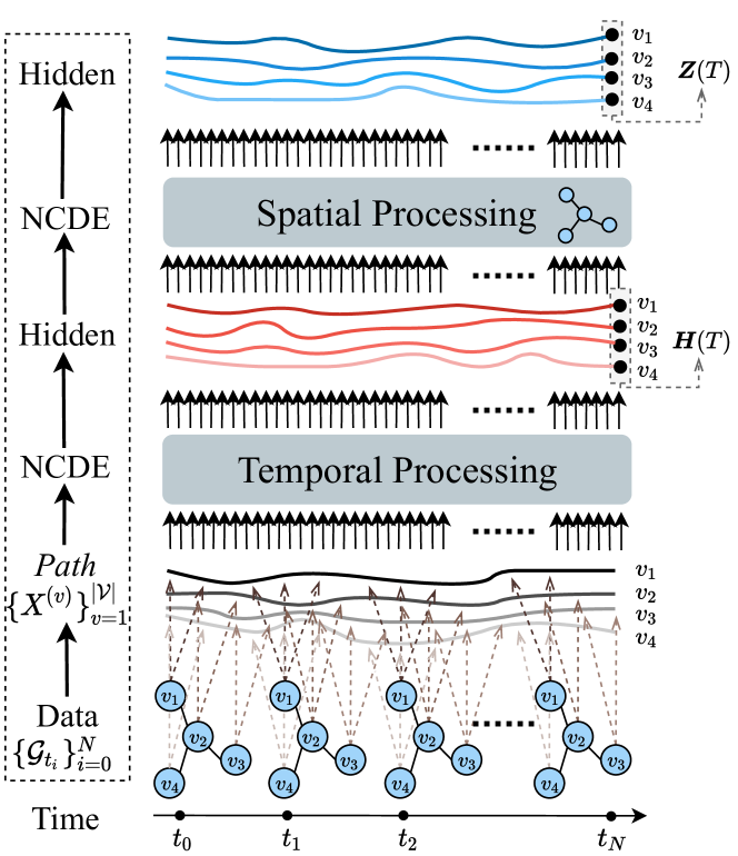
Figure 1: The overall workflow in our proposed STG-NCDE

For this task, a diverse set of techniques have been proposed. In this paper, however, we design a method based on neural controlled differential equations (NCDEs) for the first time. NCDEs, which are considered as a continuous analogue to recurrent neural networks (RNNs), can be written as follows:

$$\bm{z}(T) =\bm{z}(0)+\int_{0}^{T}f(\bm{z}(t);\bm{\theta}_{f})dX(t)$$ (1)

$$=\bm{z}(0)+\int_{0}^{T}f(\bm{z}(t);\bm{\theta}_{f})\frac{dX(t)}{dt}dt,$$ (2)

where $X$ is a continuous path taking values in a Banach space. The entire trajectory of $\bm{z}(t)$ is controlled over time by the path $X$ (cf. Fig. 2). Leaning the CDE function $f$ for a downstream task is a key point in NCDEs.

The theory of the controlled differential equation (CDE) had been developed to extend the stochastic differential equation and the Itô calculus far beyond the semimartingale setting of $X$ — in other words, Eq. (1) reduces to the stochastic differential equation if and only if $X$ meets the semimartingale requirement. For instance, a prevalent example of the path $X$ is a Wiener process in the case of the stochastic differential equation. In CDEs, however, the path $X$ does not need to be such semimartingale or martingale processes. NODEs are a technology to parameterize such CDEs and learn from data. In addition, Eq. (2) continuously reads the values $\frac{dX(t)}{dt}$ and integrates them over time. In this regard, NODEs are equivalent to continuous RNNs and show the state-of-the-art accuracy in many time-series tasks and data.

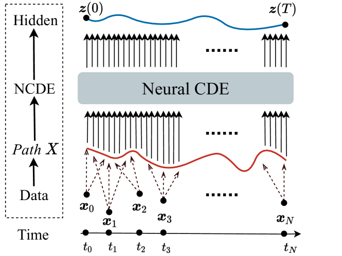
Figure 2: The overall workflow of the original NCDE for processing time-series. The path $X$ is created from $\{(t_{i},\bm{x}_{i})\}_{i=0}^{N}$ by an interpolation algorithm and therefore, this technology is robust to irregular time-series data.

However, it has not been studied yet how to combine the NCDE technology (i.e., temporal processing) and the graph convolutional processing technology (i.e., spatial processing). We integrate them into a single framework to solve the spatio-temporal forecasting problem.

In the original setting of NCDEs, there exists a single time-series, denoted $\{(t_{i},\bm{x}_{i})\}_{i=0}^{N}$, where $\bm{x}_{i}\in\mathbb{R}^{D}$ is a $D$-dimensional vector and $t_{i}$ is a time-point when $\bm{x}_{i}$ is observed. In our setting, however, there exist $|\mathcal{V}|$ different time-series patterns to consider, each of which is somehow correlated to neighboring time-series patterns. Figs. 1 and. 2 show the difference between them.

The pre-processing step in our method is to create a continuous path $X^{(v)}$ for each node $v\in\mathcal{V}$. For this, we use the same technique as that in the original NCDE design. Given a discrete time-series $\{\bm{x}_{i}\}_{i=0}^{N}$, the original NCDE runs an interpolation algorithm to build its continuous path. We apply the same method for each node separately, and a set of paths, denoted $\{X^{(v)}\}_{v=1}^{|\mathcal{V}|}$, will be created.

The main step is to jointly apply a spatial and a temporal processing method to $\{X^{(v)}\}_{v=1}^{|\mathcal{V}|}$, considering its graph connectivity. In our case, we design an NCDE model equipped with a graph processing technique for both the spatial and the temporal processing. We then derive the last hidden vector $\bm{z}^{(v)}(T)$ for each node $v$ and there is the last output layer to predict $\hat{\bm{y}}^{(v)}\in\mathbb{R}^{S\times M}$, which collectively constitutes $\hat{\bm{Y}}\in\mathbb{R}^{|\mathcal{V}|\times S\times M}$.

We conduct experiments with 6 benchmark datasets collected by California Performance of Transportation (PeMS), which are the most widely used datasets in this topic, to compare with 20 baseline methods. Our proposed method clearly outperforms all those methods in terms of three standard evaluation metrics. Our contributions can be summarized as follows:

1. We design two NCDEs for learning the temporal and spatial dependencies of traffic conditions and combine them into a single framework.

2. NCDEs are robust to irregular time-series by the design. Owing to this characteristic, our method is also robust to the irregularity of the temporal sequence, i.e., some observations can be missing.

3. Our large-scale experiments with 6 datasets and 20 baselines clearly show the efficacy of the proposed method. We, for the first time, perform irregular traffic forecasting to reflect real-world environments where sensing values can be missing (see Table 5 and Table 6).

Related Work and Preliminaries

In this section, we summarize our literature review related to our NCDE-based spatio-temporal forecasting.

Neural ordinary differential equations (NODEs)

Prior to NCDEs, neural ordinary differential equations (NODEs) introduced how to continuously model residual neural networks (ResNets) with differential equations. NODE can be written as follows:

$$\bm{z}(T)=\bm{z}(0)+\int_{0}^{T}f(\bm{z}(t),t;\bm{\theta}_{f})dt;$$ (3)

where the neural network parameterized by $\bm{\theta}_{f}$ approximates $\frac{\bm{z}(t)}{dt}$, and we rely on various ODE solvers to solve the integral problem, ranging from the explicit Euler method to the 4th order Runge–Kutta (RK4) method and the Dormand–Prince (DOPRI) method  (Dormand and Prince 1980).

In particular, Eq. (3) reduces to the residual connection when being solved by the explicit Euler method. In this regard, NODEs generalizes ResNets in a continuous manner. STGODE utilizes this NODE technology to solve the spatio-temporal forecasting problem  (Fang et al. 2021).

Neural controlled differential equations (NCDEs)

Whereas NODEs generalize ResNets, NCDEs in Eq. (1) generalize RNNs in a continuous manner. Controlled differential equations (CDEs) are a more advanced concept than ordinary differential equations (ODEs). The integral problem in Eq. (3) is a Rienmann integral problem whereas it is a Riemann–Stieltjes integral problem in Eq. (2). The original CDE formulation in Eq. (1) reduces Eq. (2) where $\frac{\bm{z}(t)}{dt}$ is approximated by $f(\bm{z}(t);\bm{\theta}_{f})\frac{dX(t)}{dt}$.

Once $\frac{\bm{z}(t)}{dt}$ is somehow successfully formulated in a close math form, we can utilize those existing ODE solvers to solve Eq. (2). Therefore, many techniques developed for solving NODEs can be applied to NCDEs as well.

Traffic forecasting

The problem of traffic forecasting is an emerging research topic in the field of spatio-temporal machine learning. When being solved in high accuracy, it has non-trivial impacts to our daily life. We introduce several milestone papers in this field. DCRNN (Li et al. 2018) combines graph convolution with recurrent neural networks in an encoder-decoder manner. STGCN (Yu, Yin, and Zhu 2018) combines graph convolution with gated temporal convolution. GraphWaveNet (Wu et al. 2019) combines adaptive graph convolution with dilated casual convolution to capture spatial-temporal dependencies. ASTGCN (Guo et al. 2019) utilizes both the spatial-temporal attention mechanism and the spatial-temporal convolution. STG2Seq (Bai et al. 2019) uses a multiple gated graph convolutional module and a seq2seq architecture with an attention mechanisms to make multi-step prediction. STSGCN (Song et al. 2020) utilizes multiple localized spatial-temporal subgraph modules to synchronously capture the localized spatial-temporal correlations directly. LSGCN (Huang et al. 2020) integrates a novel attention mechanism and graph convolution into a spatial gated block. AGCRN (Bai et al. 2020) utilizes node adaptive parameter learning to capture node-specific spatial and temporal correlations in time-series data automatically without a pre-defined graph. STFGNN (Li and Zhu 2021) captures hidden spatial-dependenies by a novel fusion operation of various spatial and temporal graphs, treated for different time periods in parallel. Z-GCNETs (Chen, Segovia-Dominguez, and Gel 2021) integrates the new time-aware zigzag topological layer into time-conditioned GCNs. STGODE (Fang et al. 2021) captures spatial-temporal dynamics through a tensor-based ODE.

Proposed Method

The spatio-temporal processing of a time-series of graphs $\{\mathcal{G}_{t_{i}}\stackrel{{\scriptstyle\text{def}}}{{=}}(\mathcal{V},\mathcal{E},\bm{F}_{i})\}_{i=0}^{N}$ is obviously more difficult than the spatial processing only (i.e., GCNs) or the temporal processing only (i.e., RNNs). As such, there have been proposed many neural networks combining GCNs and RNNs. In this paper, we design a novel spatio-temporal model based on the NCDE and the adaptive topology generation technologies. We describe our proposed method in this section. We first review its overall design and then introduce details.

Overall design

Our method includes one pre-processing and one main processing steps as follows:

1. Its pre-processing step is to create a continuous path $X^{(v)}$ for each node $v$, where $1\leq v\leq|\mathcal{V}|$, from $\{\bm{F}_{i}^{(v)}\}_{i=0}^{N}$. $\bm{F}_{i}^{(v)}\in\mathbb{R}^{D}$ means the $v$-th row of $\bm{F}_{i}$, and $\{\bm{F}_{i}^{(v)}\}$ stands for the time-series of the input features of $v$. We use the natural cubic spline method for interpolating the discrete time-series $\{\bm{F}_{i}^{(v)}\}$ and building a continuous path. Among many, the natural cubic spline has a couple of suitable characteristics to be used in our method: i) it creates a continuous path and ii) the created path is twice differentiable. In particular, the second characteristic is important when it comes to calculating the gradients of the proposed model.

2. The above pre-processing step happens before training our model. Then, our main step, which combines a GCN and an NCDE technologies, calculates the last hidden vector for each node $v$, denoted $\bm{z}^{(v)}(T)$.

3. After that, we have an output layer to predict $\hat{\bm{y}}^{(v)}\in\mathbb{R}^{S\times M}$ for each node $v$. After collecting those predictions for all nodes in $\mathcal{V}$, we have the prediction matrix $\hat{\bm{Y}}\in\mathbb{R}^{|\mathcal{V}|\times S\times M}$.

Graph neural controlled differential equations

Our proposed spatio-temporal graph neural controlled differential equation (STG-NCDE) consists of two NCDEs: one for processing the temporal information and the other for processing the spatial information.

Temporal processing

The first NCDE for the temporal processing can be written as follows:

$$\bm{h}^{(v)}(T) =\bm{h}^{(v)}(0)+\int_{0}^{T}f(\bm{h}^{(v)}(t);\bm{\theta}_{f})\frac{dX^{(v)}(t)}{dt}dt,$$ (4)

where $\bm{h}^{(v)}(t)$ is a hidden trajectory (over time $t\in[0,T]$) of the temporal information of node $v$. After stacking $\bm{h}^{(v)}(t)$ for all $v$, we can define a matrix $\bm{H}(t)\in\mathbb{R}^{|\mathcal{V}|\times\dim(\bm{h}^{(v)})}$. Therefore, the trajectory created by $\bm{H}(t)$ over time $t$ contains the hidden information of the temporal processing results. Eq. (4) can be equivalently rewritten as follows using the matrix notation:

$$\bm{H}(T) =\bm{H}(0)+\int_{0}^{T}f(\bm{H}(t);\bm{\theta}_{f})\frac{d\bm{X}(t)}{dt}dt,$$ (5)

where $\bm{X}(t)$ is a matrix whose $v$-th row is $X^{(v)}$. The CDE function $f$ separately processes each row in $\bm{H}(t)$. The key in this design is how to define the CDE function $f$ parameterized by $\bm{\theta}_{f}$. We will describe shortly how to define it. One good thing is that $f$ does not need to be a RNN. By designing it with fully-connected layers only, for instance, Eq. (5) converts it to a continuous RNN.

Spatial processing

After that, the second NCDE starts for its spatial processing as follows:

$$\begin{split}\bm{Z}(T)=\bm{Z}(0)+\int_{0}^{T}g(\bm{Z}(t);\bm{\theta}_{g})\frac{d\bm{H}(t)}{dt}dt,\end{split}$$ (6)

where the hidden trajectory $\bm{Z}(t)$ is controlled by $\bm{H}(t)$ which is created by the temporal processing.

After combining Eqs. (5) and (6), we have the following single equation which incorporates both the temporal and the spatial processing:

$$\begin{split}\bm{Z}(T)=\bm{Z}(0)+\int_{0}^{T}g(\bm{Z}(t);\bm{\theta}_{g})f(\bm{H}(t);\bm{\theta}_{f})\frac{d\bm{X}(t)}{dt}dt,\end{split}$$ (7)

where $\bm{Z}(t)\in\mathbb{R}^{|\mathcal{V}|\times\dim(\bm{z}^{(v)})}$ is a matrix created after stacking the hidden trajectory $\bm{z}^{(v)}$ for all $v$. In this NCDE, a hidden trajectory $\bm{z}^{(v)}$ is created after considering the trajectories of its neighbors — for ease of writing, we use the matrix notation in Eqs. (6) and (7). The key part is how to design the CDE function $g$ parameterized by $\bm{\theta}_{g}$ for the spatial processing.

CDE functions

We now describe the two CDE functions $f$ and $g$. The definition of $f:\mathbb{R}^{|\mathcal{V}|\times\dim(\bm{h}^{(v)})}\rightarrow\mathbb{R}^{|\mathcal{V}|\times\dim(\bm{h}^{(v)})}$ is as as follows:

$$\begin{split}f(\bm{H}(t);\bm{\theta}_{f})&=\psi(\texttt{FC}_{|\mathcal{V}|\times\dim(\bm{h}^{(v)})\rightarrow|\mathcal{V}|\times\dim(\bm{h}^{(v)})}(\bm{A}_{K})),\\ &\vdots\\ \bm{A}_{1}&=\sigma(\texttt{FC}_{|\mathcal{V}|\times\dim(\bm{h}^{(v)})\rightarrow|\mathcal{V}|\times\dim(\bm{h}^{(v)})}(\bm{A}_{0})),\\ \bm{A}_{0}&=\sigma(\texttt{FC}_{|\mathcal{V}|\times\dim(\bm{h}^{(v)})\rightarrow|\mathcal{V}|\times\dim(\bm{h}^{(v)})}(\bm{H}(t))),\end{split}$$ (8)

where $\sigma$ is a rectified linear unit, $\psi$ is a hyperbolic tangent, and $\mathtt{FC}_{input\_size\rightarrow output\_size}$ means a fully-connected layer whose input size is $input\_size$ and output size is also $output\_size$. $\bm{\theta}_{f}$ refers to the parameters of the fully-connected layers. This function $f$ independently processes each row of $\bm{H}(t)$ with the $K$ fully connected-layers.

For the spatial processing, we need to define one more CDE function $g$. The definition of $g:\mathbb{R}^{|\mathcal{V}|\times\dim(\bm{z}^{(v)})}\rightarrow\mathbb{R}^{|\mathcal{V}|\times\dim(\bm{z}^{(v)})}$ is as follows:

$$g(\bm{Z}(t);\bm{\theta}_{g}) =\psi(\texttt{FC}_{|\mathcal{V}|\times\dim(\bm{z}^{(v)})\rightarrow|\mathcal{V}|\times\dim(\bm{z}^{(v)})}(\bm{B}_{1})),$$ (9)

$$\bm{B}_{1} =(\bm{I}+\phi(\sigma(\bm{E}\cdot\bm{E}^{\intercal})))\bm{B}_{0}\bm{W}_{spatial},$$ (10)

$$\bm{B}_{0} =\sigma(\texttt{FC}_{|\mathcal{V}|\times\dim(\bm{z}^{(v)})\rightarrow|\mathcal{V}|\times\dim(\bm{z}^{(v)})}(\bm{Z}(t))),$$ (11)

where $\bm{I}$ is the $|\mathcal{V}|\times|\mathcal{V}|$ identity matrix, $\phi$ is a softmax activation, $\bm{E}\in\mathbb{R}^{|\mathcal{V}|\times C}$ is a trainable node-embedding matrix, $\bm{E}^{\intercal}$ is its transpose, and $\bm{W}_{spatial}$ is a trainable weight transformation matrix. Conceptually, $\phi(\sigma(\bm{E}\cdot\bm{E}^{\intercal}))$ corresponds to the normalized adjacency matrix $\bm{D}^{-\frac{1}{2}}\bm{A}\bm{D}^{-\frac{1}{2}}$, where $\bm{A}=\sigma(\bm{E}\cdot\bm{E}^{\intercal})$ and the softmax activation plays a role of normalizing the adaptive adjacency matrix  (Wu et al. 2019; Bai et al. 2020). We also note that Eq. (10) is identical to the first order Chebyshev polynomial expansion of the graph convolution operation (Kipf and Welling 2017) with the normalized adaptive adjacency matrix. Eqs. (9) and (11) do not mix the rows of their input matrices $\bm{Z}(t)$ and $\bm{B}_{1}$. It is Eq. (10) where the rows of $\bm{B}_{0}$ are mixed for the spatial processing.

Initial value generation

The initial value of the temporal processing, i.e., $\bm{H}(0)$, is created from $\bm{F}_{t_{0}}$ as follows: $\bm{H}(0)=FC_{D\rightarrow\dim(\bm{h}^{(v)})}(\bm{F}_{t_{0}})$. We also use the following similar strategy to generate $\bm{Z}(0)$: $\bm{Z}(0)=FC_{\dim(\bm{h}^{(v)})\rightarrow\dim(\bm{z}^{(v)})}(\bm{H}(0))$. After generating these initial values for the two NCDEs, we can calculate $\bm{Z}(T)$ after solving the Riemann–Stieltjes integral problem in Eq. (7).

How to train

To implement Eq. (7) — we do not separately implement Eqs. (5) and (6) — we define the following augmented ODE:

$$\frac{d}{dt}{\begin{bmatrix}\bm{Z}(t)\\ \bm{H}(t)\\ \end{bmatrix}\!}={\begin{bmatrix}g(\bm{Z}(t);\bm{\theta}_{g})f(\bm{H}(t);\bm{\theta}_{f})\frac{d\bm{X}(t)}{dt}\\ f(\bm{H}(t);\bm{\theta}_{f})\frac{d\bm{X}(t)}{dt}\\ \end{bmatrix}\!},$$ (12)

where the initial values $\bm{Z}(0)$ and $\bm{H}(0)$ are generated in the aforementioned ways. We then train the parameters of the initial value generation layer, the CDE functions, including the node-embedding matrix $\bm{E}$, and the output layer. From $\bm{z}^{(v)}(T)$, i.e., the $v$-th row of $\bm{Z}(T)$, the following output layer produces $\hat{\bm{y}}^{(v)}$.

$$\hat{\bm{y}}^{(v)}=\bm{z}^{(v)}(T)\bm{W}_{output}+\bm{b}_{output},$$ (13)

where $\bm{W}_{output}\in\mathbb{R}^{\dim(\bm{z}^{(v)}(T))\rightarrow S\times M}$ and $\bm{b}_{output}\in\mathbb{R}^{S\times M}$ are a trainable weight and a bias of the output layer. We use the following $L^{1}$ loss as the training objective, which is defined as:

$$\mathcal{L}=\frac{\sum_{\tau\in\mathcal{T}}\sum_{v\in\mathcal{V}}\|\bm{y}^{(\tau,v)}-\hat{\bm{y}}^{(\tau,v)}\|_{1}}{|\mathcal{V}|\times|\mathcal{T}|},$$ (14)

where $\mathcal{T}$ is a training set, $\tau$ is a training sample, and $\bm{y}^{(\tau,v)}$ is the ground-truth of node $v$ in $\tau$. We also use the standard $L^{2}$ regularization of the parameters, i.e., weight decay.

The well-posedness of NCDEs was already proved in (Lyons, Caruana, and Lévy 2007, Theorem 1.3) under the mild condition of the Lipschitz continuity. We show that our NCDE layers are also well-posed problems. Almost all activations, such as ReLU, Leaky ReLU, SoftPlus, Tanh, Sigmoid, ArcTan, and Softsign, have a Lipschitz constant of 1. Other common neural network layers, such as dropout, batch normalization and other pooling methods, have explicit Lipschitz constant values. Therefore, the Lipschitz continuity of $f$ and $g$ can be fulfilled in our case. Therefore, it is a well-posed training problem. Therefore, our training algorithm solves a well-posed problem so its training process is stable in practice.

Experiments

We describe our experimental environments and results. We conduct experiments with time-series forecasting. Our software and hardware environments are as follows: Ubuntu 18.04 LTS, Python 3.9.5, Numpy 1.20.3, Scipy 1.7, Matplotlib 3.3.1, torchdiffeq 0.2.2, PyTorch 1.9.0, CUDA 11.4, and NVIDIA Driver 470.42, i9 CPU, and NVIDIA RTX A6000. We use 6 datasets and 20 baseline models, which is one of the largest scale experiments in the field of traffic forecasting. For additional figures, tables, and best hyperparameter settings are in Appendix.

Datasets

In the experiment, we use six real-world traffic datasets, namely PeMSD7(M), PeMSD7(L), PeMS03, PeMS04, PeMS07, and PeMS08, which were collected by California Performance of Transportation (PeMS) (Chen et al. 2001) in real-time every 30 second and widely used in the previous studies (Yu, Yin, and Zhu 2018; Guo et al. 2019; Fang et al. 2021; Chen, Segovia-Dominguez, and Gel 2021; Song et al. 2020). More details of the datasets are in Table 1. We note that they contain different types of values: i) the number of vehicles, or ii) velocity.

Dataset	$|\mathcal{V}|$	Time Steps	Time Range	Type
PeMSD3	358	26,208	09/2018 - 11/2018	Volume
PeMSD4	307	16,992	01/2018 - 02/2018	Volume
PeMSD7	883	28,224	05/2017 - 08/2017	Volume
PeMSD8	170	17,856	07/2016 - 08/2016	Volume
PeMSD7(M)	228	12,672	05/2012 - 06/2012	Velocity
PeMSD7(L)	1,026	12,672	05/2012 - 06/2012	Velocity

Table 1: The summary of the datasets used in our work. We predict either traffic volume (i.e., # of vehicles) or velocity.

Experimental Settings

The datasets are already split with a ratio of 6:2:2 into training, validating, and testing sets. In these datasets, the interval between two consecutive time-points is 5 minutes. All existing papers, including our paper, use the forecasting settings of $S=12$ and $M=1$ after reading past 12 graph snapshots, i.e., $N=11$ — note that the graph snapshot index $i$ starts from $0$. In short, we conduct a 12-sequence-to-12-sequence forecasting, which is the standard benchmark setting in this domain.

We use the mean absolute error (MAE), the mean absolute percentage error (MAPE), and the root mean squared error (RMSE) to measure the performance of different models.

Baselines

We compare our proposed STG-NCDE with the following baseline models in conjunction with the previous models we introduced in the related work section — in total, we use 20 baseline models:

1. HA (Hamilton 2020) uses the average value of the last 12 times slices to predict the next value.

2. ARIMA is a statistical model of time series analysis.

3. VAR (Hamilton 2020) is a time series model that captures spatial correlations among all traffic series.

4. TCN (Bai, Kolter, and Koltun 2018) consists of a stack of causal convolutional layers with exponentially enlarged dilation factors.

5. FC-LSTM (Sutskever, Vinyals, and Le 2014) is LSTM with fully connected hidden unit.

6. GRU-ED (Cho et al. 2014) is an GRU-based baseline and utilize the encoder-decoder framework for multi-step time series prediction.

7. DSANet (Huang et al. 2019) is a correlated time series prediction model using CNN networks and self-attention mechanism for spatial correlations.

Hyperparameters

For our method, we test with the following hyperparameter configurations: we train for 200 epochs using the Adam optimizer, with a batch size of 64 on all datasets. The two dimensionalities of $\dim(\bm{h}^{(v)})$ and $\dim(\bm{z}^{(v)})$ are {32, 64, 128, 256}, the node embedding size $C$ is from 1 to 10, and the number of $K$ in Eq. (8) is in {1, 2, 3}. The learning rate in all methods is in {$1\text{\times}{10}^{-2}$, $5\text{\times}{10}^{-3}$, $1\text{\times}{10}^{-3}$, $5\text{\times}{10}^{-4}$, $1\text{\times}{10}^{-4}$} and the weight decay coefficient is in {$1\text{\times}{10}^{-4}$, $1\text{\times}{10}^{-3}$, $1\text{\times}{10}^{-2}$}. An early stop strategy with a patience of 15 iterations on the validation dataset is used. The best hyperparameters are in Appendix for reproducibility. For baselines, we run their codes with a hyperparameter search process based on their recommended configurations if their accuracy is not known for a dataset. If known, we use their officially reported accuracy.

Model	MAE	RMSE	MAPE
STGCN	14.88 (117.0%)	24.22 (113.6%)	12.30 (121.8%)
DCRNN	14.90 (117.1%)	24.04 (112.7%)	12.75 (126.1%)
GraphWaveNet	15.94 (125.3%)	26.22 (122.9%)	12.96 (128.2%)
ASTGCN(r)	14.86 (116.9%)	23.95 (112.3%)	12.25 (121.3%)
STSGCN	14.45 (113.5%)	23.58 (110.5%)	11.42 (113.0%)
AGCRN	13.32 (104.7%)	22.29 (104.5%)	10.37 (102.7%)
STFGNN	13.92 (109.5%)	22.57 (105.8%)	11.30 (111.9%)
STGODE	13.56 (106.6%)	22.37 (104.8%)	10.77 (106.6%)
Z-GCNETs	13.22 (104.0%)	21.92 (102.7%)	10.44 (103.4%)
STG-NCDE	12.72 (100.0%)	21.33 (100.0%)	10.10 (100.0%)

Table 2: The average error of some selected highly performing models across all the six datasets. Inside the parentheses, we show their performance relative to our method.

Model	PeMSD3				PeMSD4				PeMSD7				PeMSD8
	MAE	RMSE	MAPE		MAE	RMSE	MAPE		MAE	RMSE	MAPE		MAE	RMSE	MAPE
HA	31.58	52.39	33.78%		38.03	59.24	27.88%		45.12	65.64	24.51%		34.86	59.24	27.88%
ARIMA	35.41	47.59	33.78%		33.73	48.80	24.18%		38.17	59.27	19.46%		31.09	44.32	22.73%
VAR	23.65	38.26	24.51%		24.54	38.61	17.24%		50.22	75.63	32.22%		19.19	29.81	13.10%
FC-LSTM	21.33	35.11	23.33%		26.77	40.65	18.23%		29.98	45.94	13.20%		23.09	35.17	14.99%
TCN	19.32	33.55	19.93%		23.22	37.26	15.59%		32.72	42.23	14.26%		22.72	35.79	14.03%
TCN(w/o causal)	18.87	32.24	18.63%		22.81	36.87	14.31%		30.53	41.02	13.88%		21.42	34.03	13.09%
GRU-ED	19.12	32.85	19.31%		23.68	39.27	16.44%		27.66	43.49	12.20%		22.00	36.22	13.33%
DSANet	21.29	34.55	23.21%		22.79	35.77	16.03%		31.36	49.11	14.43%		17.14	26.96	11.32%
STGCN	17.55	30.42	17.34%		21.16	34.89	13.83%		25.33	39.34	11.21%		17.50	27.09	11.29%
DCRNN	17.99	30.31	18.34%		21.22	33.44	14.17%		25.22	38.61	11.82%		16.82	26.36	10.92%
GraphWaveNet	19.12	32.77	18.89%		24.89	39.66	17.29%		26.39	41.50	11.97%		18.28	30.05	12.15%
ASTGCN(r)	17.34	29.56	17.21%		22.93	35.22	16.56%		24.01	37.87	10.73%		18.25	28.06	11.64%
MSTGCN	19.54	31.93	23.86%		23.96	37.21	14.33%		29.00	43.73	14.30%		19.00	29.15	12.38%
STG2Seq	19.03	29.83	21.55%		25.20	38.48	18.77%		32.77	47.16	20.16%		20.17	30.71	17.32%
LSGCN	17.94	29.85	16.98%		21.53	33.86	13.18%		27.31	41.46	11.98%		17.73	26.76	11.20%
STSGCN	17.48	29.21	16.78%		21.19	33.65	13.90%		24.26	39.03	10.21%		17.13	26.80	10.96%
AGCRN	15.98	28.25	15.23%		19.83	32.26	12.97%		22.37	36.55	9.12%		15.95	25.22	10.09%
STFGNN	16.77	28.34	16.30%		20.48	32.51	16.77%		23.46	36.60	9.21%		16.94	26.25	10.60%
STGODE	16.50	27.84	16.69%		20.84	32.82	13.77%		22.59	37.54	10.14%		16.81	25.97	10.62%
Z-GCNETs	16.64	28.15	16.39%		19.50	31.61	12.78%		21.77	35.17	9.25%		15.76	25.11	10.01%
STG-NCDE	15.57	27.09	15.06%		19.21	31.09	12.76%		20.53	33.84	8.80%		15.45	24.81	9.92%
Only temporal	20.44	32.82	20.03%		26.31	40.97	17.95%		28.77	44.39	12.60%		20.83	32.55	13.01%
Only spatial	15.92	27.17	15.14%		19.86	31.92	13.35%		21.72	34.73	9.24%		17.58	27,76	11.27%

Table 3: Forecasting error on PeMSD3, PeMSD4, PeMSD7 and PeMSD8

Experimental Results

Tables 3 and 4 present the detailed prediction performance. Overall, our proposed method, STG-NCDE, clearly marks the best average accuracy as summarized in Table 2. For each notable model, we list its average MAE/RMSE/MAPE from the six datasets. Inside the parentheses, we also show the relative accuracy in comparison with our method. For instance, STGCN shows an MAE that is 17.0% worse than that of our method. All existing methods show worse errors in all metrics than our method (by large margins for many baselines).

We now describe experimental results in each dataset. STG-NCDE shows the best accuracy in all cases, followed by Z-GCNETs, AGCRN, STGODE and so on. There are no existing methods that are as stable as STG-NCDE. For instance, STGODE shows reasonably low errors in many cases, e.g., an RMSE of 27.84 in PeMSD3 by STGODE, which is the second best result vs. 27.09 by STG-NCDE. However, it is outperformed by AGCRN and Z-GCNETs for PeMSD7. Only our method, STG-NCDE, shows reliable predictions in all cases.

Model	PeMSD7(M)				PeMSD7(L)
	MAE	RMSE	MAPE		MAE	RMSE	MAPE
HA	4.59	8.63	14.35%		4.84	9.03	14.90%
ARIMA	7.27	13.20	15.38%		7.51	12.39	15.83%
VAR	4.25	7.61	10.28%		4.45	8.09	11.62%
FC-LSTM	4.16	7.51	10.10%		4.66	8.20	11.69%
TCN	4.36	7.20	9.71%		4.05	7.29	10.43%
TCN(w/o causal)	4.43	7.53	9.44%		4.58	7.77	11.53%
GRU-ED	4.78	9.05	12.66%		3.98	7.71	10.22%
DSANet	3.52	6.98	8.78%		3.66	7.20	9.02%
STGCN	3.86	6.79	10.06%		3.89	6.83	10.09%
DCRNN	3.83	7.18	9.81%		4.33	8.33	11.41%
GraphWaveNet	3.19	6.24	8.02%		3.75	7.09	9.41%
ASTGCN(r)	3.14	6.18	8.12%		3.51	6.81	9.24%
MSTGCN	3.54	6.14	9.00%		3.58	6.43	9.01%
STG2Seq	3.48	6.51	8.95%		3.78	7.12	9.50%
LSGCN	3.05	5.98	7.62%		3.49	6.55	8.77%
STSGCN	3.01	5.93	7.55%		3.61	6.88	9.13%
AGCRN	2.79	5.54	7.02%		2.99	5.92	7.59%
STFGNN	2.90	5.79	7.23%		2.99	5.91	7.69%
STGODE	2.97	5.66	7.36%		3.22	5.98	7.94%
Z-GCNETs	2.75	5.62	6.89%		2.91	5.83	7.33 %
STG-NCDE	2.68	5.39	6.76%		2.87	5.76	7.31%
Only temporal	3.34	6.68	8.41%		3.54	7.03	8.89%
Only spatial	2.77	5.40	7.00%		2.99	5.85	7.60%

Table 4: Forecasting error on PeMSD7(M) and PeMSD7(L)

We also visualize the ground-truth and the predicted curves by our method and Z-GCNETs in Fig. 3. Node 111 and 261 (resp. Node 9 and 112) are two of the highest traffic areas in PeMSD4 (resp. PeMSD8). Since Z-GCNETs shows reasonable performance, its predicted curve is similar to that of our method in many time-points. As highlighted with boxes, however, our method shows much more accurate predictions for challenging cases. In particular, our method significantly outperforms Z-GCNETs for the highlighted time-points for Node 111 in PeMSD4 and Node 9 in PeMSD8, for which Z-GCNETs shows nonsensical predictions, i.e., the prediction curves are straight.

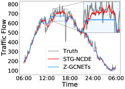
(a) Node 111 in PeMSD4

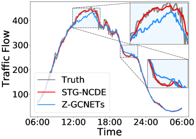
(b) Node 261 in PeMSD4

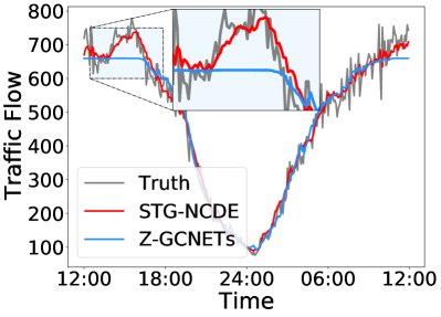
(c) Node 9 in PeMSD8

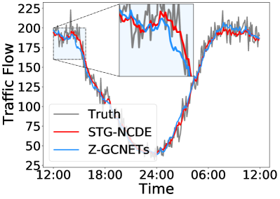
(d) Node 112 in PeMSD8

Figure 3: Traffic forecasting visualization. More visualizations in other datasets are in Appendix.

Ablation, Sensitivity, and Additional Studies

Ablation study

As ablation study models, we define the following two models: i) the first ablation model has only the temporal processing part, i.e., Eq. (5), and ii) the second ablation model has only the spatial processing part which can be written as follows:

$$\begin{split}\bm{Z}(T)=\bm{Z}(0)+\int_{0}^{T}g(\bm{Z}(t);\bm{\theta}_{g})\frac{d\bm{X}(t)}{dt}dt,\end{split}$$ (15)

where the trajectory $\bm{Z}(t)$ over time is controlled by $\bm{X}(t)$. We accordingly change the model architecture for this ablation study model. The first (resp. second) model is denoted as “Only temporal” (resp. “Only spatial”) in the tables.

In all cases, the ablation study model only with the spatial processing significantly outperforms that only with the temporal processing, e.g., an RMSE of 15.92 in PeMSD3 by the spatial processing vs. 20.44 by the temporal processing. However, STG-NCDE, which utilizes both the temporal and the spatial processing, outperforms them. This shows that we need both of them to achieve the best model accuracy.

In Fig. 4 (a), we also compare their training curves in PeMSD7. STG-NODE’s loss curve is stabilized after the second epoch whereas the other two ablation models require longer time until their loss curves are stabilized.

(a) Training curve in PeMSD7

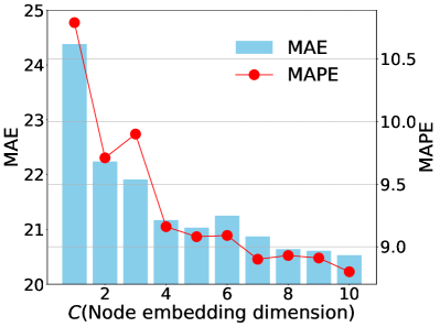
(b) Sensitivity to $C$ in PeMSD7

Figure 4: Training curve and sensitivity analysis. More results in other datasets are in Appendix.

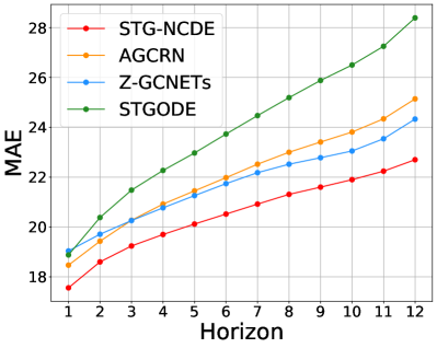
(a) MAE on PeMSD7

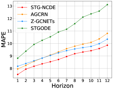
(b) MAPE on PeMSD7

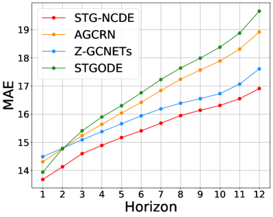
(c) MAE on PeMSD8

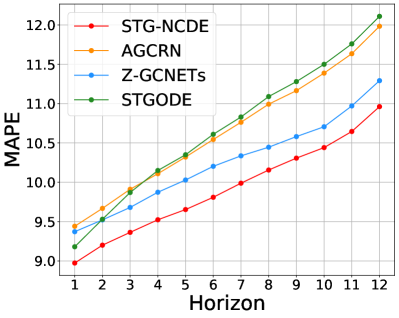
(d) MAPE on PeMSD8

Figure 5: Prediction error at each horizon. More results in other datasets are in Appendix.

Sensitivity to $C$

Fig. 4 (b) shows the MAE and MAPE by varying the node embedding size $C$. The two error metrics are stabilized after $C=7$. With $C=10$, we can achieve the best accuracy.

Error for each horizon

In our notation, $S$ denotes the length of forecasting, i.e., the number of forecasting horizons. Since the benchmark dataset has a setting of $S=12$, we show the model error for each forecasting horizon in Fig. 5. It is obvious that the error levels show a high correlation to $S$. For all horizons, STG-NCDE shows smaller errors than other baselines.

Irregular traffic forecasting

In reality, traffic sensors can be damaged and we cannot collect data in some areas for a certain amount of time. In order to reflect this situation, we randomly drop 10% to 50% of sensing values for each node independently. Since NCDEs are able to consider irregular time-series by the design, STG-NCDE is also able to do it without any changes on its model design, which is one of the most distinguishable points in comparison with existing baselines. Tables 5 and 6 summarize its results. In comparison with the results in Table 3, our model’s performance is not significantly degraded. We note that other baselines listed in Table 3 cannot do irregular forecasting and we compare STG-NCDE with its ablation models in Tables 5 and 6.

Table 5: Forecasting error on irregular PeMSD4

Model	Missing rate	MAE	RMSE	MAPE
STG-NCDE	10%	19.36	31.28	12.79%
Only Temporal		26.26	40.89	17.66%
Only Spatial		19.73	31.67	13.20%
STG-NCDE	30%	19.40	31.30	13.04%
Only Temporal		26.86	41.73	18.35%
Only Spatial		19.83	31.95	13.29%
STG-NCDE	50%	19.98	32.09	13.48%
Only Temporal		28.15	43.54	19.14%
Only Spatial		20.14	32.30	13.30%

Table 6: Forecasting error on irregular PeMSD8. More results in other datasets are in Appendix.

Model	Missing rate	MAE	RMSE	MAPE
STG-NCDE	10%	15.68	24.96	10.05%
Only Temporal		21.18	33.02	13.26%
Only Spatial		16.85	26.63	11.12%
STG-NCDE	30%	16.21	25.64	10.43%
Only Temporal		21.46	33.37	13.57%
Only Spatial		18.46	29.03	12.16%
STG-NCDE	50%	16.68	26.17	10.67%
Only Temporal		22.68	35.14	14.11%
Only Spatial		17.98	28.12	11.87%

Conclusions

We presented a spatio-temporal NCDE model to perform traffic forecasting. Our model has two NCDEs: one for temporal processing and the other for spatial processing. In particular, our NCDE for spatial processing can be considered as an NCDE-based interpretation of graph convolutional networks. In our experiments with 6 datasets and 20 baselines, our method clearly shows the best overall accuracy. In addition, our model can perform irregular traffic forecasting where some input observations can be missing, which is a practical problem setting but not actively considered by existing methods. We believe that the combination of NCDEs and GCNs is a promising research direction for spatio-temporal processing.

Appendix A Best Hyperparameters

For reproducibility, we introduce the best hyperparameter configurations for each dataset as follows:

1. In PeMSD3, we set the number of $K$ to 1 and the node embedding size $C$ to 2. The dimensionality of hidden vector is 64. The learning rate was set to $1\text{\times}{10}^{-3}$ and the weight decay was $1\text{\times}{10}^{-3}$.

2. In PeMSD4, we set the number of $K$ to 2 and the node embedding size $C$ to 8. The dimensionality of hidden vector is 64. The learning rate was set to $1\text{\times}{10}^{-3}$ and the weight decay was $1\text{\times}{10}^{-3}$.

3. In PeMSD7, we set the number of $K$ to 2 and the node embedding size $C$ to 10. The dimensionality of hidden vector is 64. The learning rate was set to $1\text{\times}{10}^{-3}$ and the weight decay was $1\text{\times}{10}^{-3}$.

4. In PeMSD8, we set the number of $K$ to 1 and the node embedding size $C$ to 2. The dimensionality of hidden vector is 32. The learning rate was set to $1\text{\times}{10}^{-3}$ and the weight decay was $1\text{\times}{10}^{-3}$.

5. In PeMSD7(M), we set the number of $K$ to 1 and the node embedding size $C$ to 10. The dimensionality of hidden vector is 32. The learning rate was set to $1\text{\times}{10}^{-3}$ and the weight decay was $1\text{\times}{10}^{-3}$.

6. In PeMSD7(L), we set the number of $K$ to 1 and the node embedding size $C$ to 10. The dimensionality of hidden vector is 32. The learning rate was set to $1\text{\times}{10}^{-3}$ and the weight decay was $1\text{\times}{10}^{-3}$.

Table 7: Forecasting error on irregular PeMSD3

Model	Missing rate	MAE	RMSE	MAPE
STG-NCDE	10%	15.89	27.61	15.83%
Only Temporal		57.15	85.11	54.38%
Only Spatial		15.85	27.24	15.22%
STG-NCDE	30%	16.08	27.78	16.05%
Only Temporal		58.47	86.33	60.39%
Only Spatial		16.18	27.61	15.18%
STG-NCDE	50%	16.50	28.52	16.03%
Only Temporal		60.29	87.86	63.17%
Only Spatial		16.75	28.64	16.00%

Table 8: Forecasting error on irregular PeMSD7

Model	Missing rate	MAE	RMSE	MAPE
STG-NCDE	10%	20.65	33.95	8.86%
Only Temporal		29.49	45.19	12.96%
Only Spatial		21.85	34.83	9.25%
STG-NCDE	30%	20.76	34.20	8.91%
Only Temporal		29.73	45.60	13.16%
Only Spatial		21.82	34.93	9.21%
STG-NCDE	50%	21.51	34.91	9.25%
Only Temporal		31.13	47.51	13.69%
Only Spatial		22.64	35.94	9.60%

Table 9: Forecasting error on irregular PeMSD7(M)

Model	Missing rate	MAE	RMSE	MAPE
STG-NCDE	10%	2.67	5.38	6.78%
Only Temporal		3.33	6.67	8.34%
Only Spatial		2.71	5.38	6.98%
STG-NCDE	30%	2.72	5.45	6.81%
Only Temporal		3.37	6.72	8.52%
Only Spatial		2.73	5.41	6.89%
STG-NCDE	50%	2.75	5.53	6.79%
Only Temporal		3.49	6.95	8.76%
Only Spatial		2.78	5.49	7.00%

Table 10: Forecasting error on irregular PeMSD7(L)

Model	Missing rate	MAE	RMSE	MAPE
STG-NCDE	10%	2.90	5.78	7.34%
Only Temporal		3.52	7.04	8.84%
Only Spatial		2.96	5.86	7.59%
STG-NCDE	30%	2.89	5.80	7.25%
Only Temporal		3.55	7.04	8.97%
Only Spatial		2.97	5.85	7.45%
STG-NCDE	50%	3.03	5.97	7.63%
Only Temporal		3.68	7.27	9.28%
Only Spatial		3.02	5.96	7.68%

Appendix B Irregular Traffic Forecasting

Tables 10 to 10 show the irregular traffic forecasting results in the remaining datasets that are not reported in our main paper.

Appendix C Sensitivity Analysis

Fig. 6 shows the MAE and MAPE by varying the node embedding size $C$ in the remaining datasets.

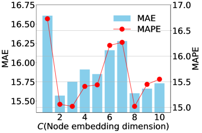
(a) PeMSD3

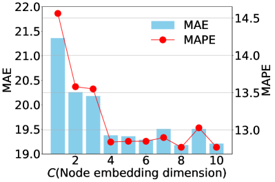
(b) PeMSD4

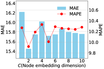
(c) PeMSD8

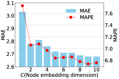
(d) PeMSD7(M)

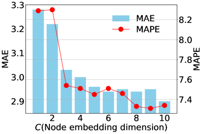
(e) PeMSD7(L)

Figure 6: Sensitivity to $C$

Appendix D Prediction Error at Each Horizon

Fig. 7 shows the prediction error at each horizon in the remaining datasets that are not reported in our main paper.

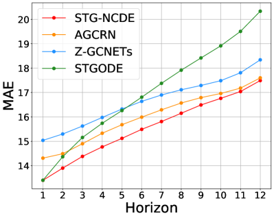
(a) MAE on PeMSD3

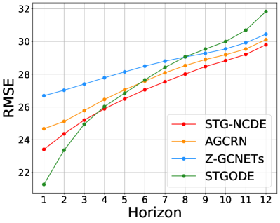
(b) RMSE on PeMSD3

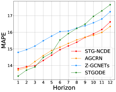
(c) MAPE on PeMSD3

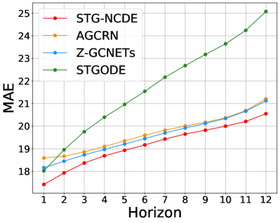
(d) MAE on PeMSD4

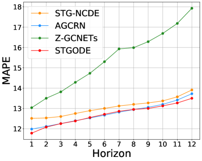
(e) MAPE on PeMSD4

(f) RMSE on PeMSD4

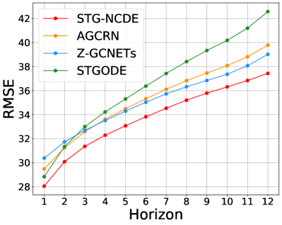
(g) RMSE on PeMSD7

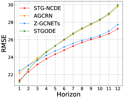
(h) RMSE on PeMSD8

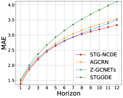
(i) MAE on PeMSD7(M)

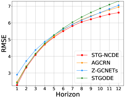
(j) MAPE on PeMSD7(M)

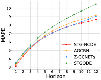
(k) RMSE on PeMSD7(M)

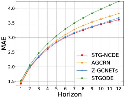
(l) MAE on PeMSD7(L)

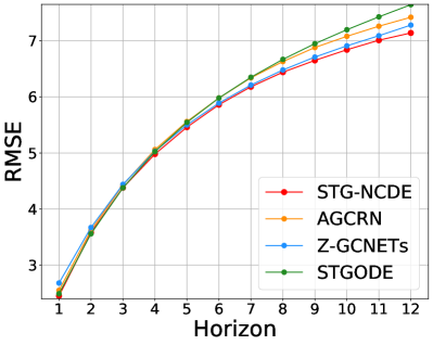
(m) MAPE on PeMSD7(L)

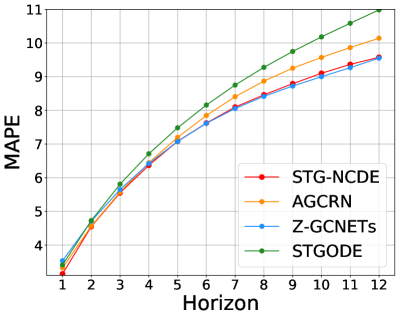
(n) RMSE on PeMSD7(L)

Figure 7: Prediction error at each horizon

Appendix E Traffic Forecasting Visualization

We also visualize the ground-truth and some forecasting outcomes by our method and Z-GCNETs in Fig. 8.

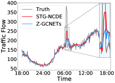
(a) Node 12 in PeMSD3

(b) Node 99 in PeMSD3

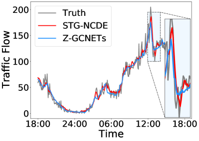
(c) Node 108 in PeMSD3

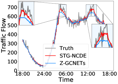
(d) Node 141 in PeMSD3

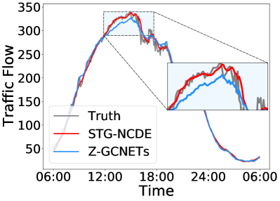
(e) Node 149 in PeMSD4

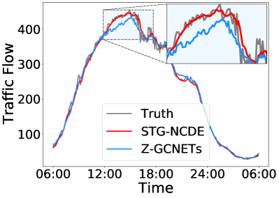
(f) Node 170 in PeMSD4

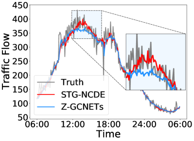
(g) Node 211 in PeMSD4

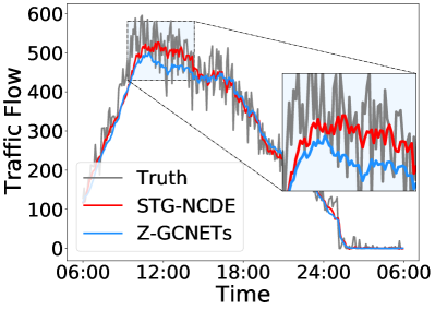
(h) Node 287 in PeMSD4

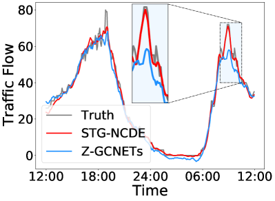
(i) Node 26 in PeMSD7

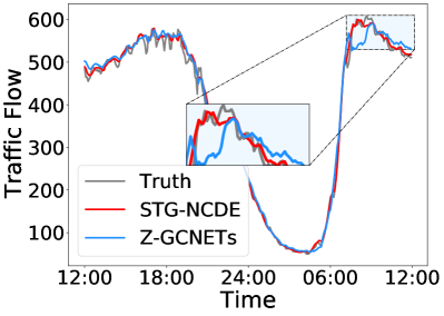
(j) Node 277 in PeMSD7

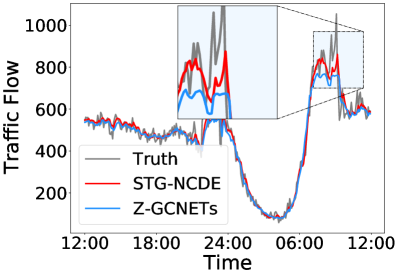
(k) Node 66 in PeMSD7

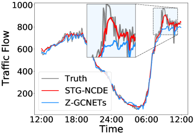
(l) Node 139 in PeMSD7

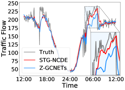
(m) Node 85 in PeMSD8

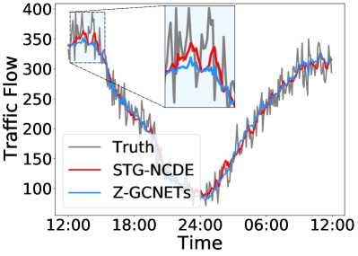
(n) Node 104 in PeMSD8

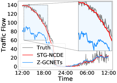
(o) Node 155 in PeMSD8

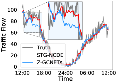
(p) Node 162 in PeMSD8

(q) Node 14 in PeMSD7(M)

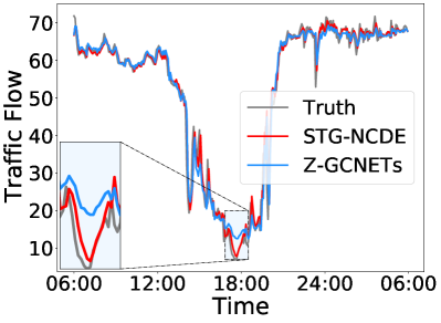
(r) Node 15 in PeMSD7(M)

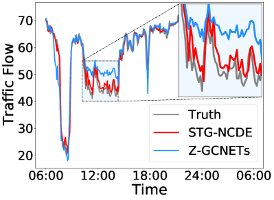
(s) Node 18 in PeMSD7(M)

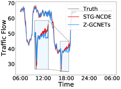
(t) Node 37 in PeMSD7(M)

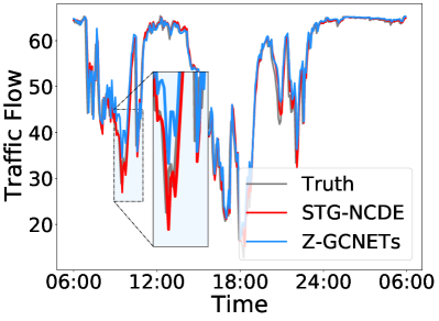
(u) Node 211 in PeMSD7(L)

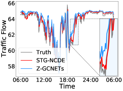
(v) Node 509 in PeMSD7(L)

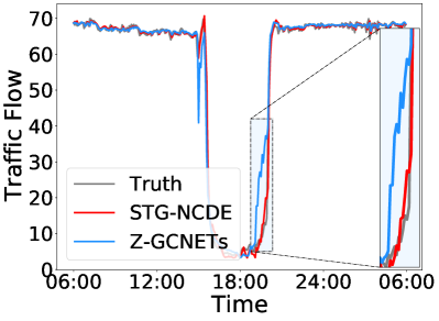
(w) Node 7009 in PeMSD7(L)

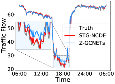
(x) Node 958 in PeMSD7(L)

Figure 8: Traffic forecasting visualization

References

- Bai et al. (2019) Bai, L.; Yao, L.; Kanhere, S. S.; Wang, X.; and Sheng, Q. Z. 2019. STG2Seq: Spatial-Temporal Graph to Sequence Model for Multi-step Passenger Demand Forecasting. In IJCAI.
- Bai et al. (2020) Bai, L.; Yao, L.; Li, C.; Wang, X.; and Wang, C. 2020. Adaptive Graph Convolutional Recurrent Network for Traffic Forecasting. In NeurIPS, volume 33, 17804–17815.
- Bai, Kolter, and Koltun (2018) Bai, S.; Kolter, J. Z.; and Koltun, V. 2018. An Empirical Evaluation of Generic Convolutional and Recurrent Networks for Sequence Modeling. arXiv:1803.01271.
- Chen et al. (2001) Chen, C.; Petty, K.; Skabardonis, A.; Varaiya, P.; and Jia, Z. 2001. Freeway performance measurement system: mining loop detector data. Transportation Research Record, 1748(1): 96–102.
- Chen, Segovia-Dominguez, and Gel (2021) Chen, Y.; Segovia-Dominguez, I.; and Gel, Y. R. 2021. Z-GCNETs: Time Zigzags at Graph Convolutional Networks for Time Series Forecasting. In ICML.
- Cheng et al. (2018a) Cheng, L.; Zang, H.; Ding, T.; Sun, R.; Wang, M.; Wei, Z.; and Sun, G. 2018a. Ensemble recurrent neural network based probabilistic wind speed forecasting approach. Energies, 11(8).
- Cheng et al. (2018b) Cheng, W.; Shen, Y.; Zhu, Y.; and Huang, L. 2018b. A neural attention model for urban air quality inference: Learning the weights of monitoring stations. In AAAI.
- Cho et al. (2014) Cho, K.; van Merrienboer, B.; Gulcehre, C.; Bougares, F.; Schwenk, H.; and Bengio, Y. 2014. Learning phrase representations using RNN encoder-decoder for statistical machine translation. In EMNLP.
- Dormand and Prince (1980) Dormand, J.; and Prince, P. 1980. A family of embedded Runge-Kutta formulae. Journal of Computational and Applied Mathematics, 6(1): 19 – 26.
- Fang et al. (2021) Fang, Z.; Long, Q.; Song, G.; and Xie, K. 2021. Spatial-Temporal Graph ODE Networks for Traffic Flow Forecasting. In KDD.
- Guo et al. (2019) Guo, S.; Lin, Y.; Feng, N.; Song, C.; and Wan, H. 2019. Attention Based Spatial-Temporal Graph Convolutional Networks for Traffic Flow Forecasting. In AAAI.
- Hamilton (2020) Hamilton, J. D. 2020. Time series analysis. Princeton university press.
- Hossain et al. (2015) Hossain, M.; Rekabdar, B.; Louis, S. J.; and Dascalu, S. 2015. Forecasting the weather of Nevada: A deep learning approach. In IJCNN.
- Huang et al. (2020) Huang, R.; Huang, C.; Liu, Y.; Dai, G.; and Kong, W. 2020. LSGCN: Long Short-Term Traffic Prediction with Graph Convolutional Networks. In IJCAI, 2355–2361.
- Huang et al. (2019) Huang, S.; Wang, D.; Wu, X.; and Tang, A. 2019. DSANet: Dual Self-Attention Network for Multivariate Time Series Forecasting. In CIKM.
- Kipf and Welling (2017) Kipf, T. N.; and Welling, M. 2017. Semi-Supervised Classification with Graph Convolutional Networks. In ICLR.
- Kurth et al. (2018) Kurth, T.; Treichler, S.; Romero, J.; Mudigonda, M.; Luehr, N.; Phillips, E.; Mahesh, A.; Matheson, M.; Deslippe, J.; Fatica, M.; et al. 2018. Exascale deep learning for climate analytics. In International Conference for High Performance Computing, Networking, Storage and Analysis. IEEE.
- Li and Zhu (2021) Li, M.; and Zhu, Z. 2021. Spatial-Temporal Fusion Graph Neural Networks for Traffic Flow Forecasting. In AAAI.
- Li et al. (2018) Li, Y.; Yu, R.; Shahabi, C.; and Liu, Y. 2018. Diffusion Convolutional Recurrent Neural Network: Data-Driven Traffic Forecasting. In ICLR.
- Liu et al. (2016) Liu, Y.; Racah, E.; Correa, J.; Khosrowshahi, A.; Lavers, D.; Kunkel, K.; Wehner, M.; Collins, W.; et al. 2016. Application of deep convolutional neural networks for detecting extreme weather in climate datasets. arXiv preprint.
- Lyons, Caruana, and Lévy (2007) Lyons, T. J.; Caruana, M.; and Lévy, T. 2007. Differential equations driven by rough paths. Springer.
- Racah et al. (2016) Racah, E.; Beckham, C.; Maharaj, T.; Kahou, S. E.; Pal, C.; et al. 2016. ExtremeWeather: A large-scale climate dataset for semi-supervised detection, localization, and understanding of extreme weather events. arXiv preprint.
- Ren et al. (2021) Ren, X.; Li, X.; Ren, K.; Song, J.; Xu, Z.; Deng, K.; and Wang, X. 2021. Deep Learning-Based Weather Prediction: A Survey. Big Data Research, 23.
- Shi et al. (2015) Shi, X.; Chen, Z.; Wang, H.; Yeung, D.-Y.; Wong, W.-K.; and Woo, W.-c. 2015. Convolutional LSTM network: A machine learning approach for precipitation nowcasting. In NeurIPS.
- Shi et al. (2017) Shi, X.; Gao, Z.; Lausen, L.; Wang, H.; Yeung, D.-Y.; Wong, W.-k.; and Woo, W.-c. 2017. Deep learning for precipitation nowcasting: A benchmark and a new model. arXiv preprint.
- Song et al. (2020) Song, C.; Lin, Y.; Guo, S.; and Wan, H. 2020. Spatial-Temporal Synchronous Graph Convolutional Networks: A New Framework for Spatial-Temporal Network Data Forecasting. In AAAI.
- Sutskever, Vinyals, and Le (2014) Sutskever, I.; Vinyals, O.; and Le, Q. V. 2014. Sequence to sequence learning with neural networks. In NeurIPS, 3104–3112.
- Tekin et al. (2021) Tekin, S. F.; Karaahmetoglu, O.; Ilhan, F.; Balaban, I.; and Kozat, S. S. 2021. Spatio-temporal Weather Forecasting and Attention Mechanism on Convolutional LSTMs. arXiv preprint.
- Wu et al. (2019) Wu, Z.; Pan, S.; Long, G.; Jiang, J.; and Zhang, C. 2019. Graph WaveNet for Deep Spatial-Temporal Graph Modeling. In IJCAI, 1907–1913.
- Yu, Yin, and Zhu (2018) Yu, B.; Yin, H.; and Zhu, Z. 2018. Spatio-Temporal Graph Convolutional Networks: A Deep Learning Framework for Traffic Forecasting. In IJCAI.
- Zaytar and El Amrani (2016) Zaytar, M. A.; and El Amrani, C. 2016. Sequence to sequence weather forecasting with long short-term memory recurrent neural networks. International Journal of Computer Applications.