ADD: Frequency Attention and Multi-View based Knowledge Distillation to Detect Low-Quality Compressed Deepfake Images

Abstract

Despite significant advancements of deep learning-based forgery detectors for distinguishing manipulated deepfake images, most detection approaches suffer from moderate to significant performance degradation with low-quality compressed deepfake images.Because of the limited information in low-quality images, detecting low-quality deepfake remains an important challenge. In this work, we apply frequency domain learning and optimal transport theory in knowledge distillation (KD) to specifically improve the detection of low-quality compressed deepfake images. We explore transfer learning capability in KD to enable a student network to learn discriminative features from low-quality images effectively. In particular, we propose the Attention-based Deepfake detection Distiller (ADD), which consists of two novel distillations: 1) frequency attention distillation that effectively retrieves the removed high-frequency components in the student network, and 2) multi-view attention distillation that creates multiple attention vectors by slicing the teacher’s and student’s tensors under different views to transfer the teacher tensor’s distribution to the student more efficiently. Our extensive experimental results demonstrate that our approach outperforms state-of-the-art baselines in detecting low-quality compressed deepfake images.

Introduction

Recently, facial manipulation techniques using deep learning methods such as deepfakes have drawn considerable attention  (Rossler et al. 2019; Pidhorskyi, Adjeroh, and Doretto 2020; Richardson et al. 2020; Nitzan et al. 2020). Moreover, deepfakes have become more realistic and sophisticated, making it difficult to be distinguished by human eyes (Siarohin et al. 2020). And it has become much easier to generate such realistic deepfakes than before. Hence, such advancements and convenience enable even novices to easily create highly realistic fake faces for simple entertainment. However, these fake images raise serious security, privacy, and social concerns, as they can be abused for malicious purposes, such as impersonation (Catherine 2019), revenge pornography (Cole 2018), and fake news propagation (Quandt et al. 2019).

To address such problems arising from deepfakes, there have been immense research efforts in developing effective deepfake detectors (Dzanic, Shah, and Witherden 2019; Rossler et al. 2019; Wang et al. 2019; Li and Lyu 2018; Khayatkhoei and Elgammal 2020; Zhang, Karaman, and Chang 2019). Most approaches utilize the deep learning-based approaches, where generally they perform well if there are a large amount of high-resolution training data. However, the performances of these approaches drop dramatically (by up to $18\%$ (Dzanic, Shah, and Witherden 2019; Rossler et al. 2019)) for compressed low-resolution images due to lack of available pixel information to sufficiently distinguish fake images from real ones. In other words, because of the compression, subtle differences and artifacts such as sharp edges in hairs and lips that can be possibly leveraged for differentiating deepfakes can also be removed. Therefore, there still remains an important challenge to effectively detect low-quality compressed deepfakes, which frequently occur on social media and mobile platforms in bandwidth-challenging and storage-limited environments.

In this work, we propose the Attention-based Deepfake detection Distiller (ADD). Our primary goal is to detect low-quality (LQ) deepfakes, which are less explored in most previous studies but plays a pivotal role in real-world scenarios. First, we assume there are high-quality (HQ) images are readily available, similar to the settings in other studies (Rossler et al. 2019; Wang et al. 2019; Li and Lyu 2018; Khayatkhoei and Elgammal 2020; Zhang, Karaman, and Chang 2019; Dzanic, Shah, and Witherden 2019). And, we use knowledge distillation (KD) as an overarching backbone architecture to detect low-quality deepfakes. While most of the existing knowledge distillation methods aim to reduce the student size for model compression applications or improve the performance of lightweight deep learning models  (Hinton, Vinyals, and Dean 2015; Tian, Krishnan, and Isola 2019; Huang and Wang 2017; Passalis and Tefas 2018), we hypothesize that a student can learn lost distinctive features of low-quality compressed images from a teacher that is pre-trained on high-quality images for deepfake detection. We first lay out the following two major challenges associated with detecting the LQ compressed deepfakes, and provide the intuitions of our approaches to overcome these issues:

1) Loss of high-frequency information. As discussed, while lossy image compression algorithms make changes visually unnoticeable to humans, they can significantly reduce DNNs’ deepfake detection capability by removing the fine-grained artifacts in high-frequency components. To investigate this phenomenon more concretely, we revisit Frequency Principal (F-Principal) (Xu, Zhang, and Xiao 2019), which describes the learning behavior of general DNNs in the frequency domain. F-Principal states that general DNNs tend to learn dominant low-frequency components first and then capture high-frequency components during the training process (Xu, Zhang, and Xiao 2019). For example, to illustrate this issue, Fig. 1 is provided to indicates that most of the lost information during compression is from high-frequency components. As a consequence, general DNNs shift their attention in later training epochs to high-frequency components, which now represent intrinsic characteristics of objects in each individual image rather than discriminative features. This learning process increases the variance of DNNs’ decision boundaries and induces overfitting, thereby degrading the detection performance. A trivial approach to tackle the overfitting is applying the early stopping method (Morgan and Bourlard 1989); however, fine-grained artifacts of deepfakes can be subsequently omitted, especially when they are highly compressed. To overcome this issue, we propose the novel frequency attention distiller, which guides the student to effectively recover the removed high-frequency components in low-quality compressed images from the teacher during training.

2) Loss of correlated information. In addition, under heavy compression, crucial features and pixel correlations that not only capture the intra-class variations, but also characterize the inter-class differences are also degraded. In particular, these correlations are essential for CNNs’ ability to learn the features at the local filters, but they are significantly removed in the compressed input images.

Recent studies (Wang et al. 2018; Hu et al. 2018) have empirically demonstrated that training DNNs that are able to capture this correlated information can successfully improve their performances. Therefore, in this work, we focus on improving the lost correlations by proposing a novel multi-view attention, inspired by the work of Bonneel et al. (Bonneel et al. 2015), and contrastive distillation (Tian, Krishnan, and Isola 2019). The element-wise discrepancy between the teacher’s and student’s tensors that ignores the relationship within local regions of pixels, or channel-wise attention that only considers a single dimension of backbone features. On the other hand, our proposed method ensures that our model attends to output tensors from multiple views (slices) using Sliced Wasserstein distance (SWD) (Bonneel et al. 2015). Therefore, our multi-view attention distiller guides the student to mimic its teacher more efficiently through a geometrically meaningful metric based on SWD. In summary, we present our overall Attention-based Deepfake detection Distiller (ADD), which consists of two novel distillations (See Fig. 2): 1) frequency attention distillation that effectively retrieves the removed high-frequency components in the student network, and 2) multi-view attention distillation that creates multiple attention vectors by slicing the teacher’s and student’s tensors under different views to transfer the teacher tensor’s distribution to the student more efficiently.

Our contributions are summarized as follows:

• We propose the novel frequency attention distillation, which effectively enables the student to retrieve high-frequency information from the teacher.

• We develop the novel multi-view attention distillation with contrastive distillation for the student to efficiently mimic the teacher while maintaining pixel correlations from the teacher to the student through SWD.

• We demonstrate that our approach outperforms well-known baselines, including attention-based distillation methods, on different low-quality compressed deepfake datasets.

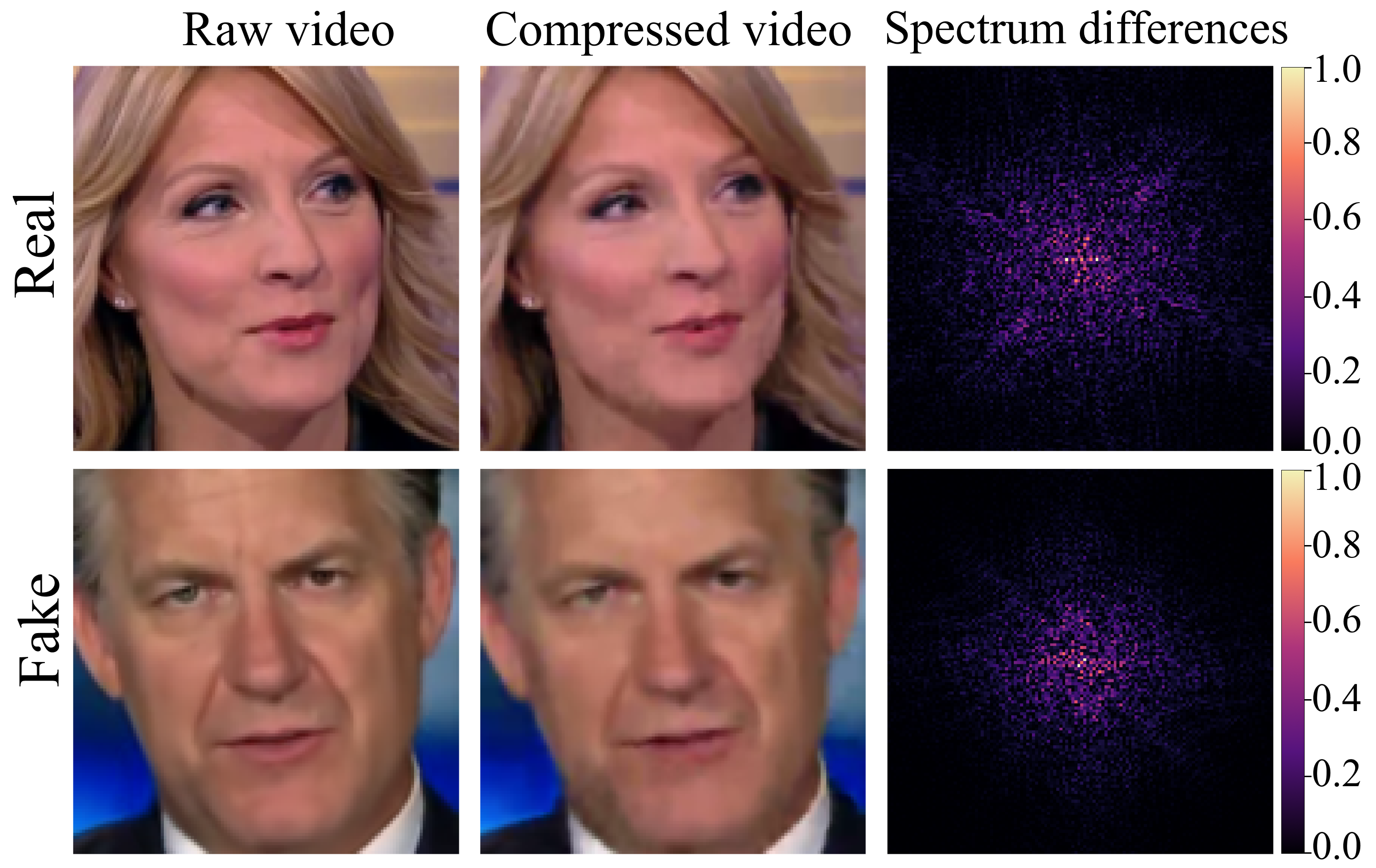
Figure 1: Degradation of high-frequency components after compression of real and fake videos. Sample fake face frames are taken from the NeuralTextures dataset in FaceForensics++ (Rossler et al. 2019). Left column: Sample faces from raw videos. Middle column: Sample faces from c40-compressed videos. Right column: Normalized spectrum differences in the frequency domain after applying Discrete Fourier Transform (DFT) to raw and compressed images. The concentrated differences at the center are the highest frequency components.

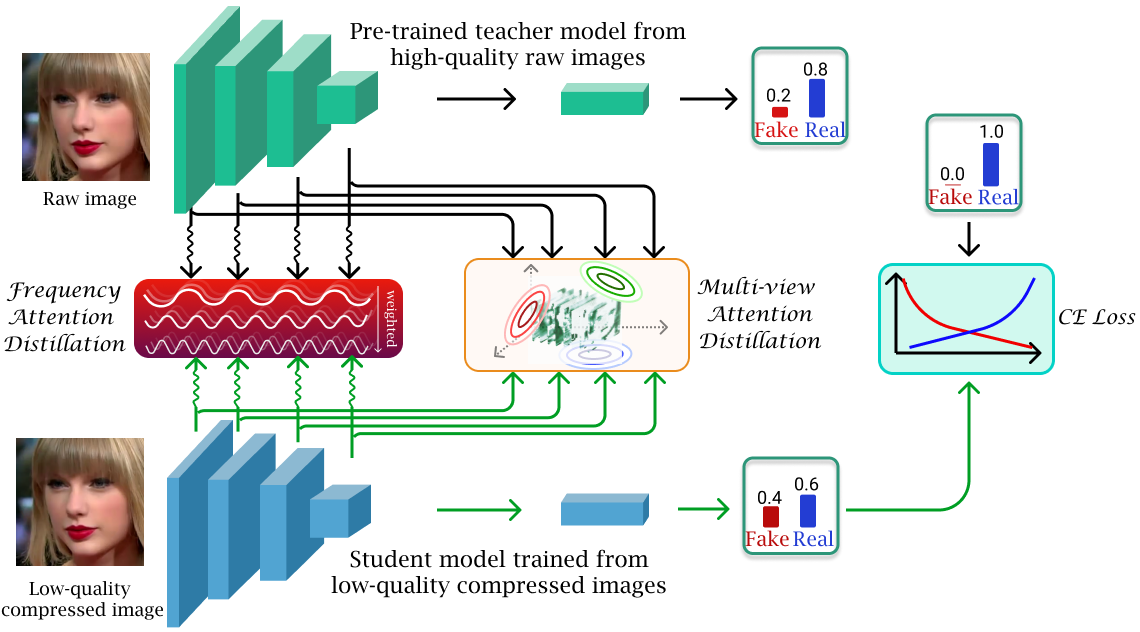
Figure 2: Illustration of our proposed Attention-based Deepfake detection Distiller (ADD) distillation framework. First, a low-quality compressed image and its corresponding raw image are used as an input to the student and pre-trained teacher model, respectively. The student model is trained with two novel distillers: 1) frequency attention distiller and 2) multi-view attention distiller. The frequency attention distiller creates a weighted loss, which focuses more on the degraded high-frequency components. The multi-view attention distiller slices student’s and teacher’s tensors by different random views to spawn multiple attention vectors. Green arrows indicate the flows of gradient decent updates to train the student’s parameters.

Related Work

Deepfake detection. Deepfake detection has recently drawn significant attention, as it is related to protecting personal privacy. Therefore, there has been a large number of research works to identify such deepfakes (Rossler et al. 2019; Li et al. 2020, 2019; Jeon et al. 2020; Rahmouni et al. 2017; Wang et al. 2019; Li and Lyu 2018). Li et al. (Li et al. 2020) tried to expose the blending boundaries of generated faces and showed the effectiveness of their method, when applied for unseen face manipulation techniques. Self-training with L2-starting point regularization was introduced by Jeon et al. (Jeon et al. 2020) to detect newly generated images. However, the majority of prior works are limited to high-quality (HQ) synthetic images, which are rather straightforward to detect by constructing binary classifiers with a large amount of HQ images.

Knowledge distillation (KD). Firstly introduced by Hinton et al. (Hinton, Vinyals, and Dean 2015), KD is a training technique that transfers acquired knowledge from a pre-trained teacher model to a student model for model compression applications. However, many existing works (Yim et al. 2017; Tian, Krishnan, and Isola 2019; Huang and Wang 2017; Passalis and Tefas 2018) applied different types of distillation methods to conventional datasets, e.g., ImageNet, PASCAL VOC 2007, and CIFAR100, but not for deepfake datasets. On the other hand, Zhu et al. (Zhu et al. 2019) used FitNets (Romero et al. 2014) to train a student model that is able to detect low-resolution images, which is similar to our method in that the teacher and the student learn to detect high and low-quality images, respectively. However, their approach coerces the student to mimic the penultimate layer’s distribution from the teacher, while it does not possess rich features at the lower layers.

In order to encourage the student model to mimic the teacher more effectively, Zagoruyko and Komodakis (Zagoruyko and Komodakis 2016) proposed the activation-based attention transfer, similar to FitNets, but their approach achieves better performance by creating spatial attention maps. Our multi-view attention method inherits from this approach but carries more generalization ability by not only exploiting spatial attention (in width and height dimension), but also introducing attention features from random dimensions using Radon transform (Helgason 2010). Thus, our approach pushes the student’s backbone features closer to the teacher’s.

In addition, inspired by InfoNCE loss (Oord, Li, and Vinyals 2018), Tian et al. (Tian, Krishnan, and Isola 2019) proposed contrastive representation distillation (CRD), which formulates the contrastive learning framework and motivates the student network to drive samples from positive pairs closer, and push away those from negative pairs. Although CRD achieves superior performance to those of previous approaches, it requires a large memory buffer to save embedding features of each sample. This is restrictive when training size and embedding space become larger. Instead, we directly sample positive and negative images in the same mini-batch and apply the contrastive loss to embedded features, similar to the Siamese network (Bromley et al. 1994).

Frequency domain learning. In the field of media forensics, several approaches (Jiang et al. 2020; Khayatkhoei and Elgammal 2020; Dzanic, Shah, and Witherden 2019) showed that discrepancies of high-frequency’s Fourier spectrum are effective clues to distinguish CNN-based generated images. Frank et al. (Frank et al. 2020) and and Zhang et al. (Zhang, Karaman, and Chang 2019) utilized the checkerboard artifacts (Odena, Dumoulin, and Olah 2016) of the frequency spectrum caused by up-sampling components of generative neural networks (GAN) as effective features in detecting GAN-based fake images. Nevertheless, their detection performances were greatly degraded when the training synthesized images are compressed, becoming low-quality. Quian et al. proposed an effective frequency-based forgery detection method, named $F^{3}Net$, which decomposes an input image to many frequency components, collaborating with local frequency statistics on a two-streams network. The $F^{3}Net$, however, doubles the number of parameters from its backbone.

Wasserstein distance. Induced by the optimal transport theory, Wasserstein distance (WD) (Villani 2008), and its variations have been explored in training DNNs to learn a particular distribution thanks to Wasserstein’s underlying geometrically meaningful distance property. In fact, WD-based applications cover a wide range of fields, such as to improve generative models (Arjovsky, Chintala, and Bottou 2017; Deshpande, Zhang, and Schwing 2018), learn the distribution of latent space in autoencoders (Kolouri et al. 2018; Xu et al. 2020), and match features in domain adaptation tasks (Lee et al. 2019).In this work, we utilize the Wasserstein metric to provide the student geometrically meaningful guidance to efficiently mimic the teacher’s tensor distribution. Thus, the student can learn the true tensor distribution, even though its input features are partially degraded through high compression.

Our Approach

Our Attention-based Deepfake detection Distiller (ADD) is consisted of the following two novel distillations (See Fig. 2): 1) frequency attention distillation and 2) multi-view attention distillation.

Frequency Attention Distillation

Let $f_{\mathcal{S}}$ and $f_{\mathcal{T}}$ be the student and the pre-trained teacher network. By forwarding a low-quality compressed input image and its corresponding raw image through $f_{\mathcal{S}}$ and $f_{\mathcal{T}}$, respectively, we obtain features $\mathcal{A}_{\mathcal{S}}$ and $\mathcal{A}_{\mathcal{T}}\in\mathbb{R}^{C\times W\times H}$ from its backbone network, which have $C$ channels, the width of $W$, and the height of $H$. To create frequency representations, Discrete Fourier Transform (DFT) $\mathfrak{F}:\mathbb{R}^{C\times W\times H}\to\mathbb{C}^{C\times W\times H}$ is applied to each channel as follows:

$$\mathfrak{F}_{\mathcal{A}_{\mathcal{S}/\mathcal{T}}}(c,u,v)=\displaystyle\sum_{x=1}^{W}\sum_{y=1}^{H}\mathcal{A}_{\mathcal{S}/\mathcal{T}}(c,x,y)\cdot e^{-i2\pi(\frac{ux}{W}+\frac{vy}{H})},$$ (1)

where $c,x$ and $y$ denote the $c_{th},x_{th}$ and $y_{th}$ slice in the channel, the width and height dimension of $\mathcal{A}_{\mathcal{S}}$ and $\mathcal{A}_{\mathcal{T}}$, respectively. Here, for convenience, we use the notation $\mathfrak{F}_{\mathcal{A}_{\mathcal{S}/\mathcal{T}}}$ to denote that the function is independently applied for both student’s and teacher’s backbone features. Then, the value at $(u,v)$ on each single feature-map $\mathfrak{F}_{\mathcal{A}_{\mathcal{S}/\mathcal{T}}}(c,:,:)$ indicates the coefficient of a basic frequency component. The difference between a pair of corresponding coefficients from the teacher and the student represents the absence of that student’s frequency component. Next, let $d:\mathbb{C}^{2}\to\mathbb{R}^{+}$ be a metric that assesses the distance between two input complex numbers and supports stochastic gradient descent. Then, the frequency loss between the teacher and student can be defined as follows:

$$\mathcal{L}_{\mathcal{FR}}=\displaystyle\sum_{c=1}^{C}\sum_{u=1}^{W}\sum_{v=1}^{H}w(u,v)\cdot d\big{(}\mathfrak{F}_{\mathcal{A}_{\mathcal{S}}}(c,u,v),\mathfrak{F}_{\mathcal{A}_{\mathcal{T}}}(c,u,v)\big{)},$$ (2)

where $w(u,v)$ is an attention weight at $(u,v)$. In this work, we utilize the exponential of the difference across channels between the teacher and student as the weight in the following way:

$$w(u,v)=exp\big{(}\gamma_{\mathcal{FR}}\cdot\frac{1}{C}\displaystyle\sum_{c=1}^{C}d(\mathfrak{F}_{\mathcal{A}_{\mathcal{S}}}(c,u,v),\mathfrak{F}_{\mathcal{A}_{\mathcal{T}}}(c,u,v))\big{)},$$ (3)

where $\gamma_{\mathcal{FR}}$ is a positive hyper-parameter that governs the exponential cumulative loss, as the student’s removed frequency increases. This design of attention weights ensures that the model focuses more on the losing high-frequency, and makes Eq. 2 partly similar to focal loss (Lin et al. 2017). Figure 3 visually illustrates our frequency loss.

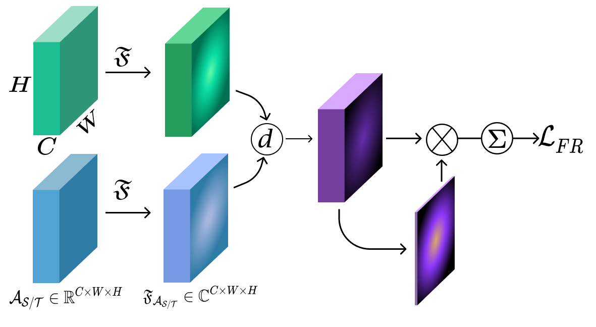
Figure 3: Illustration of our frequency attention distiller. The $\mathfrak{F}$ function is applied to each channel of the input tensor. Distance metric $d$ calculates the discrepancy of the corresponding coefficients of each frequency component from the teacher and the student. Finally, the attention map is obtained by averaging the element-wise differences across channels.

Multi-view Attention Distillation

Sliced Wasserstein distance. The p-Wasserstein distance between two probability measures $\mu$ and $\nu$ (Villani 2008) with their corresponding probability density functions $P_{\mu}$ and $P_{\nu}$ in a probability space $(\Omega,\mathcal{P}(\Omega))$ and $\Omega\subset\mathbb{R}^{d}$, is defined as follows:

$$W_{p}(P_{\mu},P_{\nu})=\Big{(}\inf_{\pi\in\Pi(\mu,\nu)}\int_{\Omega\times\Omega}\psi(x,y)^{p}d\pi(x,y)\Big{)}^{1/p},$$ (4)

where $\Pi(\mu,\nu)$ is a set of all transportation plans $\pi$, which has the marginal densities $P_{\mu}$ and $P_{\nu}$, respectively, and $\psi:\Omega\times\Omega\to\mathbb{R}^{+}$ is a transportation cost function. Equation 4 searches for an optimal transportation plan between $\mu$ and $\nu$, which is also known as Kantorovitch formulation (Kantorovitch 1958). In the case of one-dimensional probability space, i.e., $\Omega\subset\mathbb{R}$, the closed-form solution of the p-Wasserstein distance is:

$$W_{p}(P_{\mu},P_{\nu})=\Big{(}\int_{0}^{1}\psi\big{(}F_{\mu}^{-1}(\kappa),F_{\nu}^{-1}(\kappa)\big{)}^{p}\,d\kappa\Big{)}^{1/p},$$ (5)

where $F_{\mu}$ and $F_{\nu}$ are the cumulative distribution functions of $P_{\mu}$ and $P_{\nu}$, respectively.

A variation of Wasserstein distance, inspired by the above closed-form solution, is Sliced Wasserstein distance (SWD) that deploys multiple projections from a high dimensional distribution to various one-dimensional marginal distributions and calculates the optimal transportation cost for each projection. In order to construct these one-dimensional marginal distributions, we use the Radon transform (Helgason 2010), which is defined as follows:

$$\mathcal{R}_{P_{\mu}}(t,\theta)=\int_{\Omega}\mu(x)\delta(t-\langle\theta,x\rangle)dx,\forall\theta\in\mathcal{S}^{d-1},\forall t\in\mathbb{R},$$ (6)

where $\delta$ denotes the Diract delta function, $\langle\cdot,\cdot\rangle$ is the Euclidean inner-product, and $\mathcal{S}^{d-1}\subset\mathbb{R}^{d}$ is the d-dimensional unit sphere. Thus, we denote $\mathcal{R}_{\theta}\mu$ as a 1-D marginal distribution of $\mu$ under the projection on $\theta$. The Sliced 1-Wasserstein distance is defined as follows:

$$SW_{1}(P_{\mu},P_{\nu})=\int_{{S}^{d-1}}W_{1}(\mathcal{R}_{\theta}\mu,\mathcal{R}_{\theta}\nu)d\theta.$$ (7)

Now, we can calculate the Sliced Wasserstein distance by optimizing a series of 1-D transportation problems, which have the closed-form solution that can be computed in $\mathcal{O}(Nlog(N))$ (Rabin et al. 2011). In particular, by sorting $\mathcal{R}_{\theta}\mu$ and $\mathcal{R}_{\theta}\nu$ in ascending order using two permutation operators $\tau_{1}$ and $\tau_{2}$, respectively, the $SWD$ can be approximated as follows:

$$SWD(P_{\mu},P_{\nu})\approx\sum_{k=1}^{K}\sum_{i=1}^{N}\psi(\mathcal{R}_{\theta_{k}}\mu_{\tau_{1}[i]},\mathcal{R}_{\theta_{k}}\nu_{\tau_{2}[i]}),$$ (8)

where $K$ is the number of uniform random samples $\theta$ using Monte Carlo method to approximate the integration of $\theta$ over the unit sphere $\mathcal{S}^{d-1}$ in Eq. 7.

Multi-view attention distillation. Let $P_{\mathcal{A}}$ be the square of $\mathcal{A}$ after being normalized by the Frobenius norm, i.e., $P_{\mathcal{A}}=\frac{\mathcal{A}^{\circ 2}}{\|\mathcal{A}\|_{F}^{2}}$, where $\circ$ denotes the Hadamard power (Bocci, Carlini, and Kileel 2016). Consequently, we are now able to consider $P_{\mathcal{A}}$ as a discrete probability density function over $\Omega=\mathbb{R}^{C\times W\times H}\subset\mathbb{R}^{3}$, where $P_{\mathcal{A}}(c,x,y)$ indicates the density value at the slice $c_{th},x_{th}$ and $y_{th}$ of the channel, the width and height dimension, respectively. To avoid replicating the element-wise differences, we additionally need to bin the projected vectors into $g$ groups before applying distillation. One important property of our multi-view attention is that different values of $\theta$ provide different attention views (slices) of $\mathcal{A}_{\mathcal{S}}$ and $\mathcal{A}_{\mathcal{T}}$. For instance, with $\theta=(1,0,0)$, we achieve the channel-wise attention that was introduced by Chen et al. (Chen et al. 2017). Or, we can produce an attention vector in the width and height dimension, when $\theta$ becomes close to $(0,1,0)$ and $(0,0,1)$, respectively. With this general property, a student can pay full attention to its teacher’s tensor distribution instead of some pre-defined constant attention views.

Figure 4 pictorially illustrates our overall multi-view attention distillation, and we summarize our multi-view attention in Algorithm 1 in the supplementary materials. In order to encourage the semantic similarity of samples’ representation from the same class and discourage that of those from different classes, we further apply the contrastive loss for each instance, which inspired by the CRD distillation framework of Tian et al. (Tian, Krishnan, and Isola 2019) . Thus, our overall multi-view attention loss is defined as follows:

$$\begin{split}\mathcal{L}_{\mathcal{MV}}=&\gamma_{\mathcal{MV}}\times SWD(P_{\mathcal{A}_{\mathcal{S}},P_{\mathcal{A}_{\mathcal{T}}}})+\\ &\eta_{\mathcal{MV}}\times\big{[}SWD(P_{\mathcal{A}_{\mathcal{S}}},P_{\mathcal{A}^{+}_{\mathcal{T}}})+\\ &\max(\Delta-SWD\big{(}P_{\mathcal{A}_{\mathcal{S}}},P_{\mathcal{A}^{-}_{\mathcal{T}}}),0\big{)}\big{]},\end{split}$$ (9)

where $\mathcal{A}^{+}_{\mathcal{T}}$ and $\mathcal{A}^{-}_{\mathcal{T}}$ are the random instance’s representation that belong to the same and the opposite class of ${A}_{\mathcal{S}}$ at the teacher, respectively. And $\Delta$ is a margin that manages the discrepancy of negative pairs and $\gamma_{\mathcal{MV}}$, and $\eta_{\mathcal{MV}}$ are scaling hyper-parameters.

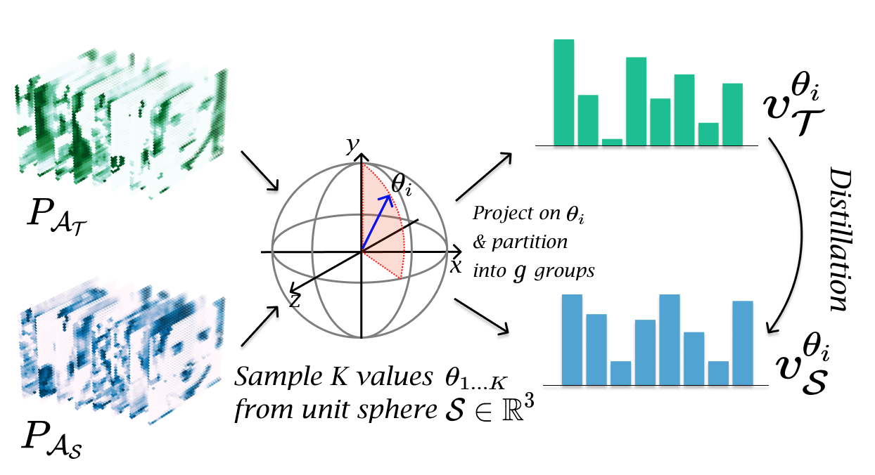
Figure 4: Detailed illustration of our multi-view attention distillation. Two backbone features of the teacher (top) and the student (bottom). After normalization, obtained features are projected on a random sample $\theta_{i}$, then two attention vectors, $v_{\mathcal{T}}^{\theta_{i}}$ and $v_{\mathcal{S}}^{\theta_{i}}$, are obtained by sorting the projection images and binning them into $g$ groups. Multiple values of $\theta$ provides us multiple attention views on the two tensors.

Overall Loss Function

The overall distillation loss in our KD framework is formulated as follows:

$$\mathcal{L}_{Distill}(A_{\mathcal{S}},A_{\mathcal{T}})=\underbrace{\alpha\cdot\mathcal{L}_{\mathcal{FR}}}_{\text{frequency attention}}+\underbrace{\beta\cdot\mathcal{L}_{\mathcal{MV}}}_{\text{multi-view attention}},$$ (10)

where $\alpha$ and $\beta$ are hyper-parameters to balance the contribution of frequency attention distiller and multi-view attention distiller, respectively. Our attention loss is parameter-free and is independent from model architecture design, and it can be directly added to any detector model’s conventional loss (e.g., cross-entropy loss). Also, the frequency attention requires computational complexity in $\mathcal{O}\big{(}CWH\cdot(log(W)+log(H))\big{)}$ for one backbone feature, where $\mathcal{O}\big{(}WH\cdot(log(W)+log(H))\big{)}$ is the complexity of 2-D Fast Fourier Transform applied for one channel. On the other hand, the average-case complexity of multi-view attention is $\mathcal{O}\big{(}KN\cdot log(N)\big{)}$, where $\mathcal{O}\big{(}N\cdot log(N)\big{)}$ is the complexity of 1-D closed-form solution as mentioned above, $K$ is the number of random samples $\theta$, and $N$ is the number of elements in one backbone feature, i.e., $N=CWH$. Our end-to-end Attention-based Deepfake detection Distiller (ADD) pipeline is presented in Fig. 2.

Experiment

Datasets

Our proposed method is evaluated on five different popular deepfake benchmark datasets: NeuralTextures (Thies, Zollhöfer, and Nießner 2019), Deepfakes (Accessed 2021-Jan-01a), Face2Face (Thies et al. 2016), FaceSwap (Accessed 2021-Jan-01c), and FaceShifter (Li et al. 2019). Every dataset has 1,000 videos generated from 1,000 real human face videos by Rössler et al. (Rossler et al. 2019). These videos are compressed into two versions: medium compression (c23) and high compression (c40), using the H.264 codec with a constant rate quantization parameter of 23, and 40, respectively. Each dataset is randomly divided into training, validation, and test set consisting of 720, 140, and 140 videos, respectively. We randomly select 64 frames from each video and obtain 92,160, 17,920, and 17,920 images for training, validation, and test set, respectively. Then, we utilize the Dblib (King 2009) to detect the largest face in every single frame and resize them to a square image of $128\times 128$ pixels.

Experiment Settings

In our experiments, we use Adam optimizer (Kingma and Ba 2014) with $\beta_{1}=0.9$, $\beta_{2}=0.999$ and $\epsilon=10^{-8}$. The learning rate is $2\times 10^{-4}$, which follows one cycle learning rate schedule (Smith and Topin 2019) with a mini-batch size of 144. In every epoch, the model is validated 10 times to save the best parameters using validation accuracy. Early stopping is applied, when the validation performance does not improve after 10 consecutive times. We use ResNet50 (He et al. 2016) as our backbone to implement our proposed distillation framework. In Eq. 2, we define $d$ as the square of the modulus of the difference between two complex number, i.e., $d(c_{1},c_{2})=|c_{1}-c_{2}|^{2}$, which satisfies the properties of a general distance metric: non-negative, symmetric, identity, and triangle inequality. The number of binning groups $g$ is equal to a half of the number of channels of $\mathcal{A}_{\mathcal{S}}$. Our hyper-parameters settings $\{\gamma_{\mathcal{FR}}=1,\gamma_{\mathcal{MV}}=100,\eta_{\mathcal{MV}}=50,\Delta=0.012,\alpha=1,\}$ are kept the same, while $\beta$ is fine-tuned on each dataset in the range of 16 to 23 through the experiments. The experiments are conducted on two TITAN RTX 24GB GPUs with Intel Xeon Gold 6230R CPU @ 2.10GHz.

Results

Our experimental results are presented in Table Results. We use Accuracy score (ACC) and Recall at 1 (R@1), which are described in detail in the supplementary materials. We compare our ADD  method, with both distillation and non-distillation baselines. For a fair comparison between different methods, the same low resolution is used at $128\times 128$ pixels as mentioned above is used throughout the experiments.

Non-distillation methods. We reproduce two highest-score deepfake detection benchmark methods  (Accessed 2021-Jan-01b): 1) the method proposed by Rössler et al.  (Rossler et al. 2019), which used Xception model, and 2) the approach by Dogonadze et al. (Dogonadze, Obernosterer, and Hou 2020), which employed Inception ResNet V1 pre-trained on the VGGFace2 dataset (Cao et al. 2018). These are the two best performing publicly available deepfake detection methods. Additionally, we use the $F^{3}Net$, which is a frequency-based deepfake detection introduced by Quian et al. (Qian et al. 2020) for evaluation. The $F^{3}Net$ is deployed on two streams of XceptionNet as described in the paper. Finally, ResNet50 (He et al. 2016) is also included as a baseline to compare with distillation methods.

Distillation baseline methods. As there has not been much research that deploys KD for deepfake detection, we further integrate other three well-known distillation architectures in the ResNet50 backbone to perform comparisons, including: FitNet (Romero et al. 2014), Attention Transfer (Zagoruyko and Komodakis 2016) (AT) and Non-local (Wang et al. 2018) (NL). Each of these methods is fine-tuned on the validation set to achieve its best performance.

First, comparing ours with the non-distillation baselines, we can observe that our method improves the detection accuracy from $1\%$ to $6\%$ across all five datasets for both compression data types. On average, our approach outperforms the other three distillation methods, and is superior on the highest compressed (c40) datasets. The model with FitNet loss, though it has a small improvement, does not have competitive results due to retaining insufficient frequency information. The attention module and non-local module also provide compelling results. However, they do not surpass our methods because of the lower attention dimension and frequency information shortage.

Datasets	Models	Medium comp- ression (c23)		High comp- ression (c40)
		ACC	R@1	ACC	R@1
NeuralTextures	Rössler et al.	76.36	57.24	56.75	51.88
	Dogonadze et al.	78.03	77.13	61.12	48.01
	$F^{3}Net$	77.91	77.39	61.95	32.35
	ResNet50	86.25	82.75	60.27	53.06
2-6	FitNet - ResNet50	86.26	84.83	66.01	57.28
	AT - ResNet50	85.21	84.99	62.61	43.50
	NL - ResNet50	88.26	86.95	65.65	46.82
	ADD - ResNet50 (ours)	88.48	87.53	68.53	58.42
DeepFakes	Rössler et al.	97.42	96.96	92.43	82.39
	Dogonadze et al.	94.67	94.39	93.97	93.52
	$F^{3}Net$	96.26	95.84	93.06	93.00
	ResNet50	96.34	95.90	92.89	91.18
2-6	FitNet - ResNet50	97.28	97.78	93.68	93.34
	AT - ResNet50	97.37	98.72	95.11	94.35
	NL - ResNet50	98.42	98.21	93.09	94.35
	ADD - ResNet50 (ours)	98.67	98.09	95.50	94.59
Face2Face	Rössler et al.	91.83	91.02	80.21	77.42
	Dogonadze et al.	89.34	88.73	83.44	81.00
	$F^{3}Net$	95.52	95.40	81.48	79.31
	ResNet50	95.60	94.77	83.94	79.88
2-6	FitNet - ResNet50	95.91	96.16	83.48	78.99
	AT - ResNet50	96.80	96.84	83.55	78.72
	NL - ResNet50	96.44	96.64	83.69	82.04
	ADD - ResNet50 (ours)	96.82	97.14	85.42	83.54
FaceSwap	Rössler et al.	95.49	95.36	88.09	87.67
	Dogonadze et al.	93.33	92.78	90.02	89.10
	$F^{3}Net$	95.74	95.65	89.58	88.90
	ResNet50	92.46	90.85	88.91	86.52
2-6	FitNet - ResNet50	97.29	96.29	89.16	90.13
	AT - ResNet50	97.66	97.27	89.75	90.41
	NL - ResNet50	97.34	96.95	91.86	90.78
	ADD - ResNet50 (ours)	97.85	97.34	92.49	92.13
FaceShifter	Rössler et al.	93.04	93.16	89.20	87.12
	Dogonadze et al.	89.80	89.36	82.03	79.96
	$F^{3}Net$	95.10	95.02	89.13	88.69
	ResNet50	94.89	93.88	89.56	88.48
2-6	FitNet - ResNet50	96.63	95.95	90.16	89.36
	AT - ResNet50	96.32	96.76	88.28	89.45
	NL - ResNet50	96.24	95.28	90.04	87.71
	ADD - ResNet50 (ours)	96.60	95.84	91.64	90.27

Table 1: Experimental results of our proposed method and other seven different baseline approaches on five different deepfake datasets. The best results are highlighted in bold.

Ablation Study and Discussions

Effects of Attention Modules. We investigate the quantitative impact of the frequency attention and multi-view attention on the final performance. In the past, the NeuralTextures (NT) dataset has shown to be the most difficult to differentiate by both human eyes and DNN (Rossler et al. 2019). Hence, we conduct our ablation study on the c40 highly NT compressed dataset. The results are presented in Table 2. We can observe that frequency attention improves about $6.76\%$ of the accuracy. Multi-view attention with contrastive loss provides a slightly better result than that of without contrastive at $68.14\%$ and $67.01\%$, respectively. Finally, combining the frequency attention and multi-view attention distillation with contrastive loss significantly improves the accuracy up to $68.53\%$. The results of our ablation study demonstrate that each proposed attention distiller has a different contribution to the student’s ability to mimic the teacher, and they are compatible when integrated together to achieve the best performance.

Model	ACC($\%$)
ResNet (baseline)	60.27
Our ResNet (FR)	67.03
Our ResNet (MV w/o contrastive)	67.01
Our ResNet (MV w/ contrastive)	68.14
Our ResNet (FR+MV)	68.53

Table 2: The effect of each single attention module on the final results experimented on NeuralTextures dataset.

Sensitivity of attention weights ($\alpha$ and $\beta$). We conduct an experiment on the sensitivity of the frequency attention weight $\alpha$ and multi-view attention weight $\beta$ on the five different datasets. The detailed results are presented in the supplementary materials. The result shows that by changing the value of $\alpha$ and $\beta$, the performance of our method continuously outperform the baseline results, indicating that our approach is less sensitive to both $\alpha$ and $\beta$.

Experiment with other backbones. Table 3 shows the results with three other backbones: ResNet18 and ResNet34 (He et al. 2016), and EfficientNet-B0 (Tan and Le 2019). We set up the hyper-parameters of the four DNNs as the same for ResNet50, except $\gamma_{\mathcal{FR}}$ is changed to $1e^{-3}$ for EfficientNet-B0. Our distilled model improves the detection accuracy of all five datasets in different compression quality, up to $7\%$, $5.8\%$ $7.1\%$ with ResNet18, ResNet34, and EfficientNet-B0 backbone compared to their baselines, respectively.

	NT		DeepFakes		Face2Face		FaceSwap		FaceShifter
	c23	c40	c23	c40	c23	c40	c23	c40	c23	c40
ResNet18
Baseline	81.8	67.3	97.5	89.2	94.2	85.0	90.2	84.5	93.2	89.2
ADD	84.3	67.5	97.7	94.7	95.7	85.3	96.0	91.5	97.0	92.2
ResNet34
Baseline	82.6	58.4	92.0	93.4	94.2	83.2	92.4	88.6	95.6	89.3
ADD	84.3	63.5	97.8	94.6	94.9	83.4	96.8	90.6	97.8	91.5
EfficientNet-B0
Baseline	81.2	60.5	96.5	90.0	94.1	77.4	92.6	83.4	93.8	84.0
ADD	83.5	67.6	97.5	92.5	96.7	80.3	95.3	87.5	95.1	85.2

Table 3: Classification accuracy $(\%)$ of ResNet18, ResNet34 and EfficientNet-B0 baseline and their integration with our ADD training framework.

Grad-CAM (Selvaraju et al. 2017). Using Grad-CAM, we provide visual explanations regarding the merits of training a LQ deepfake detector with our ADD framework. The gallery of Grad-CAM visualization is included in the supplementary material. First, our  ADD  is able to correct the facial artifacts’ attention of the LQ detector to resemble its teacher trained on raw datasets. Second, the  ADD  vigorously instructs the student model to neglect the background noises and activate the facial areas as its teacher does when encountering facial images in complex backgrounds. Meanwhile, the baseline model which is solely trained on LQ datasets steadily makes wrong predictions with high confidence by activating non-facial areas and is deceived by complex backgrounds.

Conclusion

In this paper, we proposed a novel Attention-based Deepfake detection Distillations (ADD), exploring frequency attention distillation and multi-view attention distillation in a KD framework to detect highly compressed deepfakes. The frequency attention helps the student to retrieve and focus more on high-frequency components from the teacher. The multi-view attention, inspired by Sliced Wasserstein distance, pushes the student’s output tensor distribution toward the teacher’s, maintaining correlated pixel features between tensor elements from multiple views (slices). Our experiments demonstrate that our proposed method is highly effective and achieves competitive results in most cases when detecting extremely challenging highly compressed challenging LQ deepfakes. Our code is available here.

Acknowledgments

This work was partly supported by Institute of Information & communications Technology Planning & Evaluation (IITP) grant funded by the Korea government (MSIT) (No.2019-0-00421, AI Graduate School Support Program (Sungkyunkwan University)), (No. 2019-0-01343, Regional strategic industry convergence security core talent training business) and the Basic Science Research Program through National Research Foundation of Korea (NRF) grant funded by Korea government MSIT (No. 2020R1C1C1006004). Also, this research was partly supported by IITP grant funded by the Korea government MSIT (No. 2021-0-00017, Original Technology Development of Artificial Intelligence Industry) and was partly supported by the Korea government MSIT, under the High-Potential Individuals Global Training Program (2020-0-01550) supervised by the IITP.

* Supplementary materials

Appendix A A. Multi-View Attention Algorithm

Algorithm 1 presents the pseudo-code for multi-view attention distillation between two corresponding backbone features using the Sliced Wasserstein distance (SWD) from the student and teacher models. For implicity, we formulate how each single projection $\theta_{i}$ contributes to the total SWD. However, in practice, $K$ uniform vectors $\theta_{i}$ in $\mathcal{S}^{d-1}$ can be sampled simultaneously by deep learning libraries, e.g. TensorFlow or PyTorch, and the projection operation or binning can be vertorized.

Algorithm 1 Multi-view attention distillation using the Sliced Wasserstein distance (SWD)

1:Two backbone features $\mathcal{A}_{\mathcal{S}}$ and $\mathcal{A}_{\mathcal{T}}$, which are the respective low-quality compressed and raw images from the student and teacher networks, the number of random projections $K$, and the number of bins $g$.

2:$P_{\mathcal{A}_{\mathcal{S}}}$,   $P_{\mathcal{A}_{\mathcal{T}}}$    $\leftarrow$    $\frac{\mathcal{A}_{\mathcal{S}}^{\circ 2}}{\|\mathcal{A}_{\mathcal{S}}\|_{F}^{2}}$,   $\frac{\mathcal{A}_{\mathcal{T}}^{\circ 2}}{\|\mathcal{A}_{\mathcal{T}}\|_{F}^{2}}$ $\triangleright$ normalize $\mathcal{A}_{\mathcal{S}}$ and $\mathcal{A}_{\mathcal{T}}$

3:$SWD\leftarrow 0$ $\triangleright$ initialize SWD to zero

4:for iteration $i\leftarrow 1$ to $K$ do

5:     $\theta_{i}$   $\leftarrow$   $\mathcal{U}(\mathcal{S}^{d-1})$$\triangleright$ uniformly sample $\theta_{i}$ from unit sphere in $\mathbb{R}^{3}$

6:     $u_{\mathcal{S}}^{\theta_{i}}$,   $u_{\mathcal{T}}^{\theta_{i}}$   $\leftarrow$    $\mathcal{R}_{\theta_{i}}P_{\mathcal{A}_{\mathcal{S}}}$,   $\mathcal{R}_{\theta_{i}}P_{\mathcal{A}_{\mathcal{T}}}$ $\triangleright$ project $P_{\mathcal{A}_{\mathcal{S}}}$ and $P_{\mathcal{A}_{\mathcal{T}}}$ on $\theta_{i}$

7:     ${u}_{\mathcal{S},\tau_{1}}^{\theta_{i}}$,   ${u}_{\mathcal{T},\tau_{2}}^{\theta_{i}}$   $\leftarrow$   $Sort(u_{\mathcal{S}}^{\theta_{i}})$,   $Sort(u_{\mathcal{T}}^{\theta_{i}})$ $\triangleright$ sort $u_{\mathcal{S}}^{\theta_{i}}$ and $u_{\mathcal{T}}^{\theta_{i}}$ in ascending order

8:     $v_{\mathcal{S}}^{\theta_{i}}$,   $v_{\mathcal{T}}^{\theta_{i}}$   $\leftarrow$   $\mathcal{G}({u}_{\mathcal{S},\tau_{1}}^{\theta_{i}})$,   $\mathcal{G}({u}_{\mathcal{T},\tau_{2}}^{\theta_{i}})$ $\triangleright$ partition ${u}_{\mathcal{S},\tau_{1}}^{\theta_{i}}$ and ${u}_{\mathcal{T},\tau_{2}}^{\theta_{i}}$ into $g$ bins

9:     $SWD\leftarrow SWD+\sum_{j=1}^{g}\psi(v_{\mathcal{S}}^{\theta_{i}}[j],v_{\mathcal{T}}^{\theta_{i}}[j])$ $\triangleright$ apply 1-D transportation cost with quadratic loss $\psi$

10:end for

11:return $SWD$

Appendix B B. Datasets

We describe the five different deepfake datasets used in our experiments:

• NeuralTextures. Facial reenactment is an application of Neural Textures (Thies, Zollhöfer, and Nießner 2019) technique that is used in video re-renderings. This approach includes learned feature maps stored on top of 3D mesh proxies, called neural textures, and a deferred neural renderer. The NeuralTextures datasets used in our experiment includes facial modifications of mouth regions, while the other face regions remain the same

DeepFakes. The DeepFakes dataset is generated using two autoencoders with a shared encoder, each of which is trained on the source and target faces, respectively. Fake faces are generated by decoding the source face’s embedding representation with the target face’s decoder. Note that DeepFakes, at the beginning, was a specific facial swapping technique, but is now referred to as AI-generated facial manipulation methods.

Face2Face. Face2Face (Thies et al. 2016) is a real-time facial reenactment approach, in which the target person’s expression follows the source person’s, while his/her identity is preserved. Particularly, the identity corresponding to the target face is recovered by a non-rigid model-based bundling approach on a set of key-frames that are manually selected in advance. The source face’s expression coefficients are transferred to the target, while maintaining environment lighting as well as target background.

FaceSwap. FaceSwap (Accessed 2021-Jan-01c) is a lightweight application that is built upon the graphic structures of source and target faces. A 3D model is designed to fit 68 facial landmarks extracted from the source face. Then, it projects the facial regions back to the target face by minimizing the pair-wise landmark errors and applies color correction in the final step.

FaceShifter. FaceShifter (Li et al. 2019) is a two-stage face swapping framework. The first stage includes a encoder-based multi-level feature extractor used for a target face and a generator that has Adaptive Attentional Denormalization (AAD) layers. In particular, AAD is able to blend the identity and the features to a synthesized face. In the second stage, they developed a novel Heuristic Error Acknowledging Refinement Network in order to enhance facial occlusions.

Appendix C C. Distillation Baseline Methods

In our experiement, we actively integrate three well-known distillation losses into the teacher-student training framework for comparing with ours:

• FitNet (Romero et al. 2014). FitNet method proposed hints algorithms, in which the student’s guided layers try to predict the outputs of teacher’s hint layers. We apply this hint-based learning approach on the penultimate layer of the teacher and student.

• Attention Transfer (Zagoruyko and Komodakis 2016) (AT). Attention method transfers attention maps, which are obtained by summing up spatial values across the backbone features’ channels from the teacher to the student.

• Non-local (Wang et al. 2018) (NL). Non-local module generates self-attention features from the student and teacher’s backbone features. Subsequently, the student’s self-attention tensors attempt to mimic the teacher’s.

Appendix D D. Evaluation Metrics

The results in our experiments are evaluated based on the following metrics:

• Accuracy (ACC). ACC is widely used to evaluate a classifier’s performance, and it calculates the proportion of samples whose true classes are predicted with the highest probability. ACC of a model $f_{\theta}$ tested on a test set of $N$ samples $\{(x_{1},y_{1}),...,(x_{N},y_{N})\}$ is formulated as follows:

  $$ACC=\frac{\sum_{i=1}^{N}I\left(\operatorname*{arg\,max}(f_{\theta}(x_{i})),y_{i}\right)}{N},$$ (11)

  where $I(\cdot,\cdot)$ is the Kronecker delta function.

• Recall at $k$ ($R@k$). $R@k$ indicates the proportion of test samples with at least one observed sample from the same class in $k-$nearest neighbors determined in a particular feature space. A small $R@k$ implies small intra-class variation, which usually leads to better accuracy. $R@k$ is formulated as follows:

  $$R@k=\left(1-\frac{\sum_{i=1}^{N}I\left(\sum_{j=1}^{k}I\left(neighbor_{x_{i}}[j],y_{i}\right),0\right)}{N}\right),$$ (12)

  where $neighbor_{x_{i}}[j]$ is the label of the $j^{th}$ nearest neighbor of $x_{i}$, and $I(\cdot,\cdot)$ is the Kronecker delta function. We use the Euclidean distance to measure the distances between queried and referenced samples whose features are the penultimate layer’s outputs, and we adopt $R@1$ which considers the first nearest neighbor of a test sample.

Appendix E E. Hyperparameters’ Sensitivity

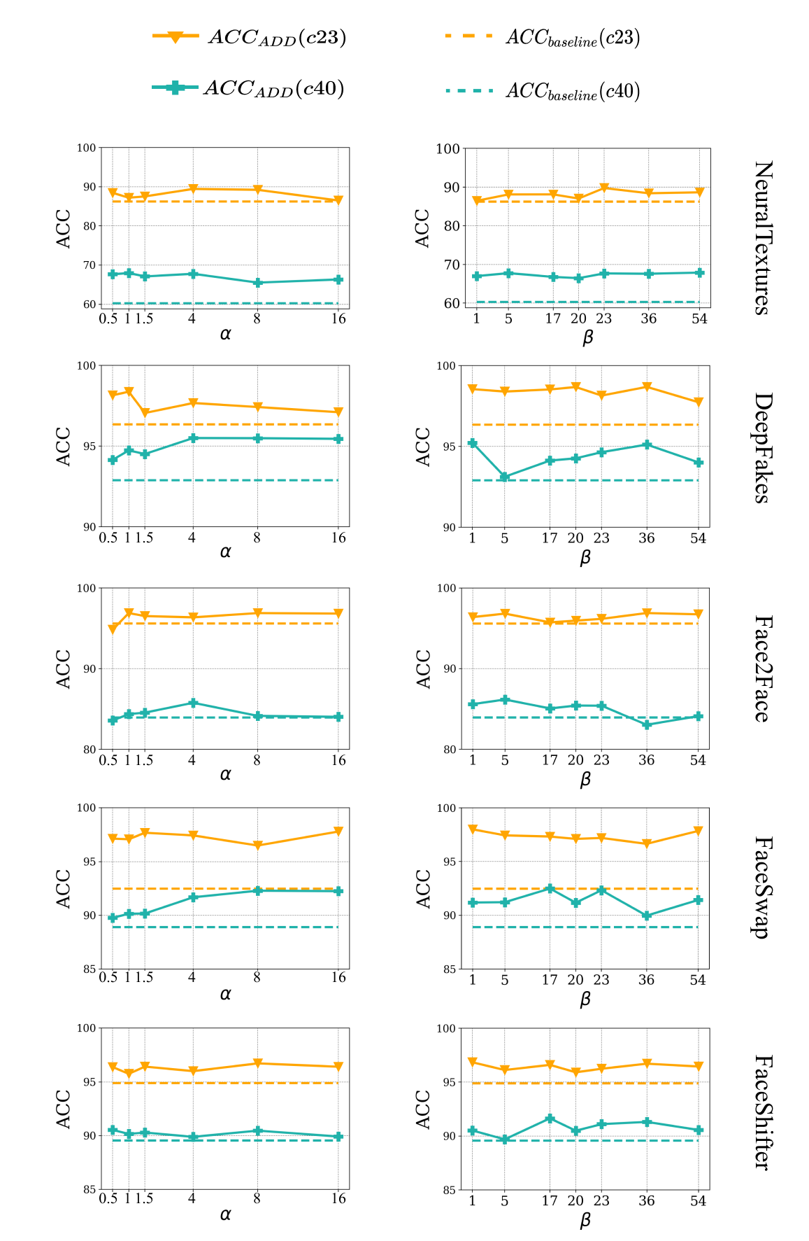
Figure 5: Ablation study on attention weights $\alpha$ (left column) and $\beta$ (right column). The blue and orange lines indicate results with medium compression (c23) and high compression (c40) data, respectively. The solid and dashed lines represent results of our  ADD - ResNet50 student model and the ResNet50 baseline model, respectively.

We examine the sensitivity of the different choices of attention weight hyperparameters, $\alpha$ and $\beta$. We experiment and show that our approach (solid lines) is less sensitive to $\alpha$ and $\beta$, and almost always outperforms the ResNet50 baselines (dashed lines) across all datasets, as shown in Fig. 5. In this work, we fix $\alpha=1$ and fine-tune $\beta$, but they can be further tuned to optimize the performance.

Appendix F F. Gallery of Grad-CAM for the Teacher, Student and Baseline Model

Grad-CAM (Selvaraju et al. 2017) is generated by back-propagating the gradients of the highest-probability class to a preceding convolutional layer’s output, producing a weighted combination with that output. The localization heat map visually indicates a particular contribution of each region to the final class prediction. The strong activation regions, which are represented in red color, are resulted from positive layer’s outputs and higher value of the gradients, whereas negative pixels or low gradients produce less activation regions are indicated in blue color. In our experiments, we utilized ResNet50 pre-trained on raw data as the teacher, our ADD - ResNet50 trained on low-quality compressed data (c40) as the student, and ResNet50 trained on the c40 data alone without any KD method as a baseline for comparison. We provide visual explanations regarding the two benefits of training a low-quality deepfake detector with our ADD framework as follows:

• Correctly identifying facial activation regions. Despite being trained on low-quality compressed images, the ResNet50 baseline still makes wrong predictions with high confidence as shown in the second column of Fig. 6. The areas pointed by red arrows indicate the baselines’ activation regions, which are different from the teacher’s, indicated by green arrows in the third column. After training with our ADD framework, the student is able to produce correct predictions that are strongly correlated and can be further visualized by its activation regions which are closely following the teacher’s.

• Resolving background confusion. Figure 7 presents the Grad-CAMs for the fake class of five different datasets, the selected samples of which have complex backgrounds. We can observe that when the teacher is trained with raw data, it produces predictions (around 1.00) with nearly perfect confidence for the fake class. When encountered highly compressed images with complex backgrounds, the ResNet50 baseline model makes wrong predictions, not activating the facial regions but the background (red arrows in Fig. 7). On the other hand, our ADD - ResNet50 model is also trained on low-quality compressed data, but our approach accumulates more distilled knowledge from the teacher and it is able to correctly identify and emphasize the actual facial areas, as its teacher similarly does with raw images (green arrows in Fig. 7).

  As shown in Fig. 7, we can demonstrate and conclude that when a low-quality compressed image has a complex background, it is easy for a conventional learning model trained without additional information (the second column) to become more vulnerable, making incorrect predictions with high confidence, activating background regions. Meanwhile, with our KD framework, the student is trained under the guidance of its teacher that can focus more on the facial areas, and effectively eliminate the background effects from the real and fake faces.

  Interestingly, as shown in Fig. 7, the baseline classifier can possibly be susceptible to and exploited by adversarial attacks, which typically add small amount of noise to the image. Therefore, one can explore the possibility of performing adversarial attacks on the compressed images by adding small amount of noise to or disordering the background. These changes resulting from adversarial attacks would be difficult to be distinguished by humans and can easily deceive the output of the baseline classifier. Therefore, it would be interesting to explore adversarial attacks for complex, compressed images and videos. Also, as a defense mechanism, we can consider KD as a framework with our novel attention mechanism for future work to better detect face regions and increase robustness against complex background noise as shown in Fig. 7.

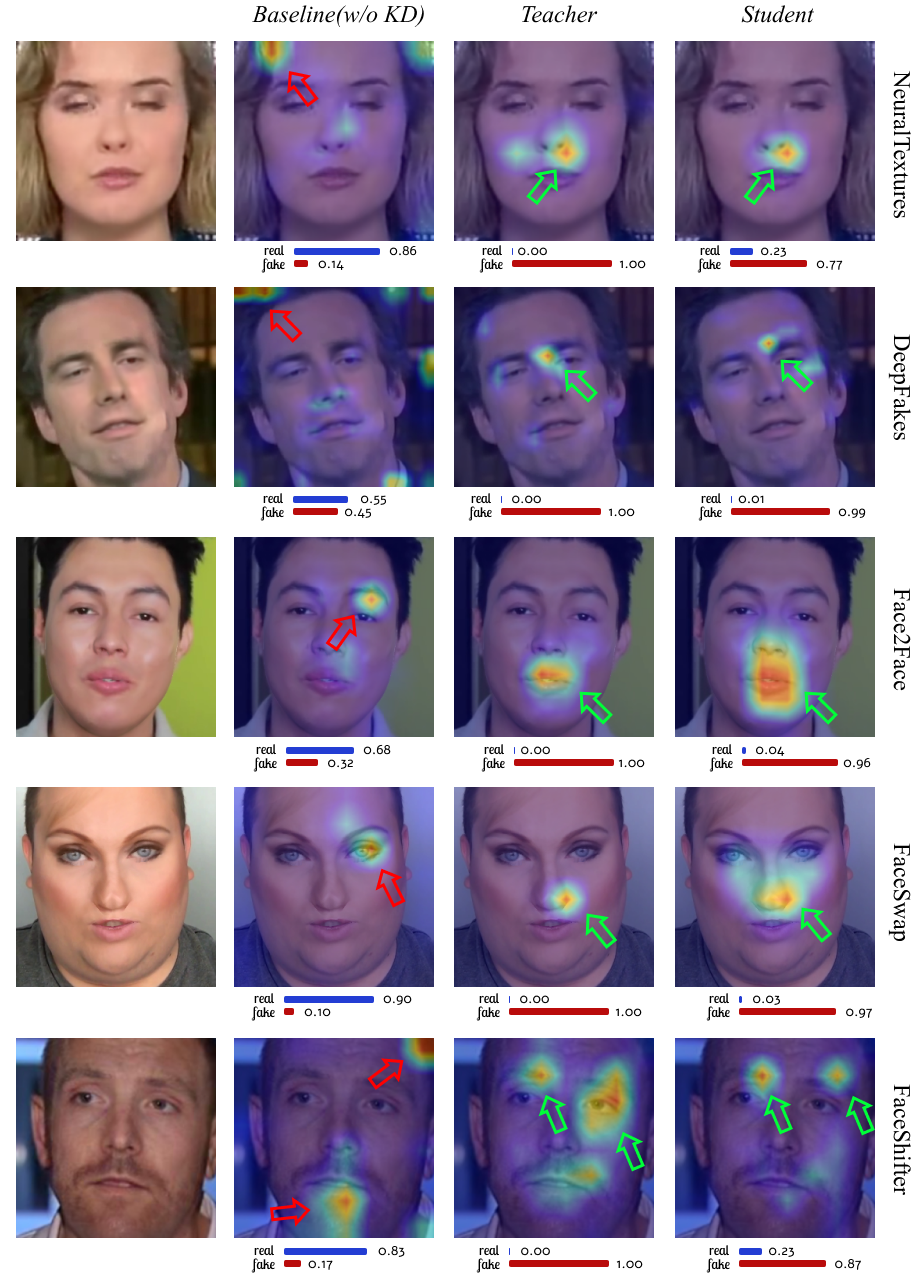
Figure 6: Grad-CAM outputs of deepfake images from NeuralTextures, DeepFakes, Face2Face, FaceSwap and FaceShifter dataset. The strongest activation regions are highlighted in red, where the blue indicates the more silent ones. The red arrows indicate the activation regions that lead to wrong predictions of ResNet50 baseline trained on highly compressed datasets without our KD framework. Green arrows in the fourth column indicate the facial activation regions of the student, which almost match with the teacher’s in the third columns, resulting from distilling knowledge from the teacher effectively by our ADD framework. (Figure is best viewed in color).

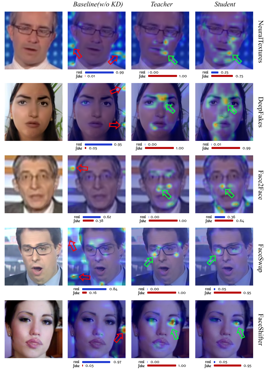
Figure 7: Class activation maps of deepfake images from NeuralTextures, DeepFakes, Face2Face, FaceSwap and FaceShifter dataset. The green arrows shown the correct facial activation regions that the student successfully mimic its teacher. The red arrows indicate non-facial areas that ResNet50 baseline relies on to make the wrong predictions with high confidence when trained on highly compressed datasets. (Figure is best viewed in color).

References

- Accessed (2021-Jan-01a) Accessed. 2021-Jan-01a. DeepFakes GitHub. https://github.com/deepfakes/faceswap.
- Accessed (2021-Jan-01b) Accessed. 2021-Jan-01b. FaceForensics Benchmark. http://kaldir.vc.in.tum.de/faceforensics˙benchmark/.
- Accessed (2021-Jan-01c) Accessed. 2021-Jan-01c. FaceSwap GitHub. https://github.com/MarekKowalski/FaceSwap/.
- Arjovsky, Chintala, and Bottou (2017) Arjovsky, M.; Chintala, S.; and Bottou, L. 2017. Wasserstein generative adversarial networks. In International conference on machine learning, 214–223. PMLR.
- Bocci, Carlini, and Kileel (2016) Bocci, C.; Carlini, E.; and Kileel, J. 2016. Hadamard products of linear spaces. Journal of Algebra, 448: 595–617.
- Bonneel et al. (2015) Bonneel, N.; Rabin, J.; Peyré, G.; and Pfister, H. 2015. Sliced and radon wasserstein barycenters of measures. Journal of Mathematical Imaging and Vision, 51(1): 22–45.
- Bromley et al. (1994) Bromley, J.; Guyon, I.; LeCun, Y.; Säckinger, E.; and Shah, R. 1994. Signature verification using a” siamese” time delay neural network. Advances in neural information processing systems, 737–737.
- Cao et al. (2018) Cao, Q.; Shen, L.; Xie, W.; Parkhi, O. M.; and Zisserman, A. 2018. Vggface2: A dataset for recognising faces across pose and age. In 2018 13th IEEE international conference on automatic face & gesture recognition (FG 2018), 67–74. IEEE.
- Catherine (2019) Catherine, S. 2019. Fraudsters Used AI to Mimic CEO’s Voice in Unusual Cybercrime Case. https://www.wsj.com/articles/fraudsters-use-ai-to-mimic-ceos-voice-in-unusual-cybercrime-case-11567157402.
- Chen et al. (2017) Chen, L.; Zhang, H.; Xiao, J.; Nie, L.; Shao, J.; Liu, W.; and Chua, T.-S. 2017. Sca-cnn: Spatial and channel-wise attention in convolutional networks for image captioning. In Proceedings of the IEEE conference on computer vision and pattern recognition, 5659–5667.
- Cole (2018) Cole, S. 2018. We Are Truly Fucked: Everyone Is Making AI-Generated Fake Porn Now.
- Deshpande, Zhang, and Schwing (2018) Deshpande, I.; Zhang, Z.; and Schwing, A. G. 2018. Generative modeling using the sliced wasserstein distance. In Proceedings of the IEEE conference on computer vision and pattern recognition, 3483–3491.
- Dogonadze, Obernosterer, and Hou (2020) Dogonadze, N.; Obernosterer, J.; and Hou, J. 2020. Deep Face Forgery Detection. arXiv preprint arXiv:2004.11804.
- Dzanic, Shah, and Witherden (2019) Dzanic, T.; Shah, K.; and Witherden, F. 2019. Fourier Spectrum Discrepancies in Deep Network Generated Images. arXiv preprint arXiv:1911.06465.
- Frank et al. (2020) Frank, J.; Eisenhofer, T.; Schönherr, L.; Fischer, A.; Kolossa, D.; and Holz, T. 2020. Leveraging frequency analysis for deep fake image recognition. In International Conference on Machine Learning, 3247–3258. PMLR.
- He et al. (2016) He, K.; Zhang, X.; Ren, S.; and Sun, J. 2016. Deep residual learning for image recognition. In Proceedings of the IEEE conference on computer vision and pattern recognition, 770–778.
- Helgason (2010) Helgason, S. 2010. Integral geometry and Radon transforms. Springer Science & Business Media.
- Hinton, Vinyals, and Dean (2015) Hinton, G.; Vinyals, O.; and Dean, J. 2015. Distilling the knowledge in a neural network. arXiv preprint arXiv:1503.02531.
- Hu et al. (2018) Hu, H.; Gu, J.; Zhang, Z.; Dai, J.; and Wei, Y. 2018. Relation networks for object detection. In Proceedings of the IEEE Conference on Computer Vision and Pattern Recognition, 3588–3597.
- Huang and Wang (2017) Huang, Z.; and Wang, N. 2017. Like what you like: Knowledge distill via neuron selectivity transfer. arXiv preprint arXiv:1707.01219.
- Jeon et al. (2020) Jeon, H.; Bang, Y.; Kim, J.; and Woo, S. S. 2020. T-GD: Transferable GAN-generated Images Detection Framework. arXiv preprint arXiv:2008.04115.
- Jiang et al. (2020) Jiang, L.; Dai, B.; Wu, W.; and Loy, C. C. 2020. Focal Frequency Loss for Generative Models. arXiv preprint arXiv:2012.12821.
- Kantorovitch (1958) Kantorovitch, L. 1958. On the translocation of masses. Management science, 5(1): 1–4.
- Khayatkhoei and Elgammal (2020) Khayatkhoei, M.; and Elgammal, A. 2020. Spatial Frequency Bias in Convolutional Generative Adversarial Networks. arXiv preprint arXiv:2010.01473.
- King (2009) King, D. E. 2009. Dlib-ml: A machine learning toolkit. The Journal of Machine Learning Research, 10: 1755–1758.
- Kingma and Ba (2014) Kingma, D. P.; and Ba, J. 2014. Adam: A method for stochastic optimization. arXiv preprint arXiv:1412.6980.
- Kolouri et al. (2018) Kolouri, S.; Pope, P. E.; Martin, C. E.; and Rohde, G. K. 2018. Sliced Wasserstein auto-encoders. In International Conference on Learning Representations.
- Lee et al. (2019) Lee, C.-Y.; Batra, T.; Baig, M. H.; and Ulbricht, D. 2019. Sliced wasserstein discrepancy for unsupervised domain adaptation. In Proceedings of the IEEE/CVF Conference on Computer Vision and Pattern Recognition, 10285–10295.
- Li et al. (2019) Li, L.; Bao, J.; Yang, H.; Chen, D.; and Wen, F. 2019. Faceshifter: Towards high fidelity and occlusion aware face swapping. arXiv preprint arXiv:1912.13457.
- Li et al. (2020) Li, L.; Bao, J.; Zhang, T.; Yang, H.; Chen, D.; Wen, F.; and Guo, B. 2020. Face x-ray for more general face forgery detection. In Proceedings of the IEEE/CVF Conference on Computer Vision and Pattern Recognition, 5001–5010.
- Li and Lyu (2018) Li, Y.; and Lyu, S. 2018. Exposing deepfake videos by detecting face warping artifacts. arXiv preprint arXiv:1811.00656.
- Lin et al. (2017) Lin, T.-Y.; Goyal, P.; Girshick, R.; He, K.; and Dollár, P. 2017. Focal loss for dense object detection. In Proceedings of the IEEE international conference on computer vision, 2980–2988.
- Morgan and Bourlard (1989) Morgan, N.; and Bourlard, H. 1989. Generalization and parameter estimation in feedforward nets: Some experiments. Advances in neural information processing systems, 2: 630–637.
- Nitzan et al. (2020) Nitzan, Y.; Bermano, A.; Li, Y.; and Cohen-Or, D. 2020. Face identity disentanglement via latent space mapping. ACM Transactions on Graphics (TOG), 39(6): 1–14.
- Odena, Dumoulin, and Olah (2016) Odena, A.; Dumoulin, V.; and Olah, C. 2016. Deconvolution and checkerboard artifacts. Distill (2016).
- Oord, Li, and Vinyals (2018) Oord, A. v. d.; Li, Y.; and Vinyals, O. 2018. Representation learning with contrastive predictive coding. arXiv preprint arXiv:1807.03748.
- Passalis and Tefas (2018) Passalis, N.; and Tefas, A. 2018. Learning deep representations with probabilistic knowledge transfer. In Proceedings of the European Conference on Computer Vision (ECCV), 268–284.
- Pidhorskyi, Adjeroh, and Doretto (2020) Pidhorskyi, S.; Adjeroh, D. A.; and Doretto, G. 2020. Adversarial latent autoencoders. In Proceedings of the IEEE/CVF Conference on Computer Vision and Pattern Recognition, 14104–14113.
- Qian et al. (2020) Qian, Y.; Yin, G.; Sheng, L.; Chen, Z.; and Shao, J. 2020. Thinking in frequency: Face forgery detection by mining frequency-aware clues. In European Conference on Computer Vision, 86–103. Springer.
- Quandt et al. (2019) Quandt, T.; Frischlich, L.; Boberg, S.; and Schatto-Eckrodt, T. 2019. Fake news. The international encyclopedia of Journalism Studies, 1–6.
- Rabin et al. (2011) Rabin, J.; Peyré, G.; Delon, J.; and Bernot, M. 2011. Wasserstein barycenter and its application to texture mixing. In International Conference on Scale Space and Variational Methods in Computer Vision, 435–446. Springer.
- Rahmouni et al. (2017) Rahmouni, N.; Nozick, V.; Yamagishi, J.; and Echizen, I. 2017. Distinguishing computer graphics from natural images using convolution neural networks. In 2017 IEEE Workshop on Information Forensics and Security (WIFS), 1–6. IEEE.
- Richardson et al. (2020) Richardson, E.; Alaluf, Y.; Patashnik, O.; Nitzan, Y.; Azar, Y.; Shapiro, S.; and Cohen-Or, D. 2020. Encoding in style: a stylegan encoder for image-to-image translation. arXiv preprint arXiv:2008.00951.
- Romero et al. (2014) Romero, A.; Ballas, N.; Kahou, S. E.; Chassang, A.; Gatta, C.; and Bengio, Y. 2014. Fitnets: Hints for thin deep nets. arXiv preprint arXiv:1412.6550.
- Rossler et al. (2019) Rossler, A.; Cozzolino, D.; Verdoliva, L.; Riess, C.; Thies, J.; and Nießner, M. 2019. Faceforensics++: Learning to detect manipulated facial images. In Proceedings of the IEEE/CVF International Conference on Computer Vision, 1–11.
- Selvaraju et al. (2017) Selvaraju, R. R.; Cogswell, M.; Das, A.; Vedantam, R.; Parikh, D.; and Batra, D. 2017. Grad-cam: Visual explanations from deep networks via gradient-based localization. In Proceedings of the IEEE international conference on computer vision, 618–626.
- Siarohin et al. (2020) Siarohin, A.; Lathuilière, S.; Tulyakov, S.; Ricci, E.; and Sebe, N. 2020. First order motion model for image animation. arXiv preprint arXiv:2003.00196.
- Smith and Topin (2019) Smith, L. N.; and Topin, N. 2019. Super-convergence: Very fast training of neural networks using large learning rates. In Artificial Intelligence and Machine Learning for Multi-Domain Operations Applications, volume 11006, 1100612. International Society for Optics and Photonics.
- Tan and Le (2019) Tan, M.; and Le, Q. 2019. Efficientnet: Rethinking model scaling for convolutional neural networks. In International Conference on Machine Learning, 6105–6114. PMLR.
- Thies, Zollhöfer, and Nießner (2019) Thies, J.; Zollhöfer, M.; and Nießner, M. 2019. Deferred neural rendering: Image synthesis using neural textures. ACM Transactions on Graphics (TOG), 38(4): 1–12.
- Thies et al. (2016) Thies, J.; Zollhofer, M.; Stamminger, M.; Theobalt, C.; and Nießner, M. 2016. Face2face: Real-time face capture and reenactment of rgb videos. In Proceedings of the IEEE conference on computer vision and pattern recognition, 2387–2395.
- Tian, Krishnan, and Isola (2019) Tian, Y.; Krishnan, D.; and Isola, P. 2019. Contrastive representation distillation. arXiv preprint arXiv:1910.10699.
- Villani (2008) Villani, C. 2008. Optimal transport: old and new, volume 338. Springer Science & Business Media.
- Wang et al. (2019) Wang, R.; Ma, L.; Juefei-Xu, F.; Xie, X.; Wang, J.; and Liu, Y. 2019. Fakespotter: A simple baseline for spotting ai-synthesized fake faces. arXiv preprint arXiv:1909.06122, 2.
- Wang et al. (2018) Wang, X.; Girshick, R.; Gupta, A.; and He, K. 2018. Non-local neural networks. In Proceedings of the IEEE conference on computer vision and pattern recognition, 7794–7803.
- Xu et al. (2020) Xu, H.; Luo, D.; Henao, R.; Shah, S.; and Carin, L. 2020. Learning autoencoders with relational regularization. In International Conference on Machine Learning, 10576–10586. PMLR.
- Xu, Zhang, and Xiao (2019) Xu, Z.-Q. J.; Zhang, Y.; and Xiao, Y. 2019. Training behavior of deep neural network in frequency domain. In International Conference on Neural Information Processing, 264–274. Springer.
- Yim et al. (2017) Yim, J.; Joo, D.; Bae, J.; and Kim, J. 2017. A gift from knowledge distillation: Fast optimization, network minimization and transfer learning. In Proceedings of the IEEE Conference on Computer Vision and Pattern Recognition, 4133–4141.
- Zagoruyko and Komodakis (2016) Zagoruyko, S.; and Komodakis, N. 2016. Paying more attention to attention: Improving the performance of convolutional neural networks via attention transfer. arXiv preprint arXiv:1612.03928.
- Zhang, Karaman, and Chang (2019) Zhang, X.; Karaman, S.; and Chang, S.-F. 2019. Detecting and simulating artifacts in gan fake images. In 2019 IEEE International Workshop on Information Forensics and Security (WIFS), 1–6. IEEE.
- Zhu et al. (2019) Zhu, M.; Han, K.; Zhang, C.; Lin, J.; and Wang, Y. 2019. Low-resolution visual recognition via deep feature distillation. In ICASSP 2019-2019 IEEE International Conference on Acoustics, Speech and Signal Processing (ICASSP), 3762–3766. IEEE.