Tensor network approach to the two-dimensional fully frustrated XY model and a chiral ordered phase

Abstract

A general framework is proposed to solve the two-dimensional fully frustrated XY model for the Josephson junction arrays in a perpendicular magnetic field. The essential idea is to encode the ground-state local rules induced by frustrations in the local tensors of the partition function. The partition function is then expressed in terms of a product of one-dimensional transfer matrix operator, whose eigen-equation can be solved by an algorithm of matrix product states rigorously. The singularity of the entanglement entropy for the one-dimensional quantum analogue provides a stringent criterion to distinguish various phase transitions without identifying any order parameter a prior. Two very close phase transitions are determined at $T_{c1}\approx 0.4459$ and $T_{c2}\approx 0.4532$, respectively. The former corresponding to a Berezinskii-Kosterlitz-Thouless phase transition describing the phase coherence of XY spins, and the latter is an Ising-like continuous phase transition below which a chirality order with spontaneously broken $Z_{2}$ symmetry is established.

I Introduction

It is well-known that the Berezinskii-Kosterlitz-Thouless (BKT) mechanismBerezinsky (1971); Kosterlitz and Thouless (1973) provides a prototypical example of topological phase transitions in two-dimensional (2D) systems and has been extensively investigated in various systems. The phase coherence of Cooper pairs in 2D superconductivity can be characterized by the BKT transition, corresponding to the unbinding vortices and anti-vortices. One of the prototype models is the two-dimensional XY model, and an attractive platform to realize the XY model is Josephson junction arraysResnick et al. (1981); Abraham et al. (1982); van Wees et al. (1987); Fazio and van der Zant (2001); Newrock et al. (2000); Cosmic et al. (2020a), where the XY spin variables represent the superconducting order-parameter phases. When applying a perpendicular magnetic field such that the flux density per plaquette is just one-half fluxvan der Zant et al. (1991); Ling et al. (1996); Martinoli and Leemann (2000); Cosmic et al. (2020b), we have the so-called fully frustrated XY model (FFXY).

The FFXY model was proposed originally as a continuum version of spin glasses possessing competing ferromagnetic and antiferromagnetic interactionsVillain (1977a, b). Although the model is $U(1)$ invariant, a new $Z_{2}$ degree of freedom emerges as a result of minimization of local conflict interactions. Due to the presence of strong frustration, extensive studies has been carried out for the FFXY model on the square latticeTeitel and Jayaprakash (1983); Thijssen and Knops (1990); Ramirez-Santiago and José (1992); Granato and Nightingale (1993); Lee (1994); Lee and Lee (1994); Ramirez-Santiago and José (1994); Olsson (1995); Cataudella and Nicodemi (1996); Olsson (1997); Boubcheur and Diep (1998); Hasenbusch et al. (2005); Okumura et al. (2011); Nussinov (2014); Lima et al. (2019) or the antiferromagnetic XY spin model on the triangular latticeMiyashita and Shiba (1984); Shih and Stroud (1984); Lee et al. (1984, 1986); Korshunov and Uimin (1986); Van Himbergen (1986); Xu and Southern (1996); Lee and Lee (1998); Capriotti et al. (1998). The nature of the phase transitions in the 2D FFXY has been the subject of a long controversy, because two distinct types of ordering occur extremely closed to each otherTeitel and Jayaprakash (1983). Despite much effort has been dedicated to the study of this model, there is not yet a general consensus on the critical behavior of these systemsOkumura et al. (2011); Lima et al. (2019).

Due to the ground state degeneracies, the study of strongly correlated statistical systems with frustrations has proven to be really difficult and most sampling methods suffer from a critical slowing down when approaching the low temperature phaseWolff (1989). Recently, an increasing interest has been stimulated on the investigation of tensor network methods in the study of the frustrated systems. It is found that, although the tensor network methods provide an effective computational approach to study the classical lattice modelsVerstraete et al. (2008); Orús (2014), special attention should be paid in the construction of the local tensors in the presence of geometrical frustrations, which has been demonstrated in the simulations of frustrated classical spin systems with discrete degrees of freedomVanderstraeten et al. (2018); Vanhecke et al. (2021). The key point is that the ground state local rules induced by frustrations should be encoded in the local tensors when comprising the whole tensor network of the partition function.

In this work, we apply the state-of-art tensor network method to study such strongly frustrated spin systems in the thermodynamic limit. It is demonstrated that the extension of the applicability of tensor networks to the fully frustrated systems with continuous $U(1)$ degrees of freedom is nontrivial, because the standard formulation of the tensor network fails to converge. Here we propose a new construction strategy based on the splitting of $U(1)$ spins, and then the partition function of the FFXY model is transformed into an infinite 2D tensor network with an enlarged unit cell, which can be efficiently contracted by a recently proposed tensor network algorithmNietner et al. (2020) under optimal variational principlesZauner-Stauber et al. (2018); Vanderstraeten et al. (2019a).

As the partition function is written in terms of a product of 1D transfer matrix operator, the singularity of the entanglement entropy of this 1D quantum transfer operator can be used to determine various phase transitions with great accuracyHaegeman and Verstraete (2017). The distinct advantage of the tensor network method over the Monte Carlo simulations is that a stringent criterion can be used to distinguish various phase transitions without identifying any order parameter a prior. From the perspective of the quantum entanglement, we can resolve the puzzles about the FFXY model with a clear evidence that the Ising phase transition takes place at a higher temperature $T_{Ising}$ than the BKT transition $T_{BKT}$. The finite-temperature phase diagram is displayed in Fig. 1(b). The low temperature phase is characterized by a long-range ordered checkerboard pattern of chirality together with a quasi-long-range XY spin order. In the intermediate temperature region ($T_{BKT}<T<T_{Ising}$), the long-range chiral order survives while the spin-spin correlations are destroyed.

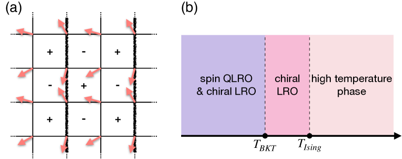
Figure 1: (a) The ground state of the fully frustrated XY model on the square lattice. The $\pm$ signs denote the checkerboard like chiralities. Thick lines correspond to $A_{ij}=\pi$ and thin lines to $A_{ij}=0$. (b) The finite-temperature phase diagram of the FFXY model showing a low temperature phase with XY spin quasi-long-range order (QLRO) and chiral long-range order (LRO), a chiral ordered phase with XY spin disorder, and a high temperature disordered phase. Two different transitions happen at $T_{BKT}\simeq 0.4459$ and $T_{Ising}\simeq 0.4459$ belonging to the BKT and Ising universality class, respectively.

The paper is organized as follows. In Sec. II we give an introduction of the 2D FFXY model and the possible phase transitions. In Sec. III we develop a general framework of the tensor network theory for this fully frustrated model. In Sec. IV we present the numerical results for the determination of the finite temperature phase diagram. Finally in Sec. V, we discuss the nature of the intermediate temperature phase and give our conclusions.

II Fully frustrated XY model

The fully frustrated XY model on a 2D square lattice can be defined by the Hamiltonian

$$H=-J\sum_{\langle ij\rangle}\cos\left(\theta_{i}-\theta_{j}+A_{ij}\right),$$ (1)

to describe the Josephson junction array under an external magnetic fieldTeitel and Jayaprakash (1983); van der Zant et al. (1991), where $J>0$ is the coupling strength, $i$ and $j$ enumerate the lattice sites, and the summation is over the pairs of the nearest neighbors. The frustration is induced by the gauge field defined on the lattice bond satisfying $A_{ij}=-A_{ji}$. The gauge field is related to the vector potential of the external magnetic field by $A_{ij}=\frac{2\pi}{\Phi_{0}}\int_{\vec{r}_{i}}^{\vec{r}_{j}}d\vec{l}\cdot\vec{A}$, where $\Phi_{0}=\frac{hc}{2e}$ is the flux quantum. The case of full frustration corresponds to the $Z_{2}$ gauge field (half quantum flux per plaquette), i.e., $\sum_{\langle i,j\rangle\in\Box}A_{ij}=\pi$, where the sum is taken around the perimeter of a plaquette.

The ground states of the FFXY model on a square lattice presents a $U(1)\times Z_{2}$ degeneracyVillain (1977a, b). The $U(1)$ degeneracy is related to the global invariance of the Hamiltonian like the 2D XY model. The two-fold discrete degeneracy is resulted from the $Z_{2}$ symmetry of the Hamiltonian under the simultaneous reversal in the signs of all $\theta_{i}$ and $A_{ij}$. The ground state is characterized by a checkerboard pattern of chiralities in analogy to the antiferromagnetic Ising model, where the planar spins rotate clockwise and counterclockwise alternatively around the plaquettes. As shown in Fig. 1(a), the chiralities $\tau=\pm 1$ are defined on the faces of the plaquettes where the corresponding gauge invariant phase differences between two nearest neighbor spins are $\varphi_{ij}\equiv\theta_{i}-\theta_{j}+A_{ij}=\pm\pi/4$. Since all the choices of fully frustrated gauge fields are physically equivalent, the gauge field given in Fig. 1(a) are used throughout this paper. In the Coulomb gas language, the $\tau_{p}=\pm 1$ chiralities can be viewed as $q_{p}=\pm\frac{1}{2}$ topological charges located at the centers of the plaquettes.

As the temperature increases, two kinds of topological excitations are expected to disorder the system: (i) point-like defects as vortices or anti-vortices which destroy the $U(1)$ phase coherence by flipping the signs of the topological charges, (ii) linear defects as the domain walls separating two ground states of different checkerboard patterns of topological charges. Hence, the FFXY model is expected to have two kinds of phase transitions associated with the formation of the quasi-long-range order of the $U(1)$ spins and the long-range Ising order characterized by chirality. Besides, the close interplay between different topological excitations makes it difficult but interesting to explore the nature of the transitions.

III Tensor network theory

III.1 Representations of partition function

The partition function of a classical lattice model with local interactions can be always represented as a contraction of tensor network on its original lattice. The standard construction of the network starts from putting an interaction matrix on each bond accounting for the Boltzmann weight. Then the local tensors defined on the lattice sites are obtained by taking suitable decompositions for the local bond matrices. Although this paradigm has been proven a success in the studies of the classical XY modelYu et al. (2014); Vanderstraeten et al. (2019b); Song and Zhang (2021a), it cannot be directly applied to the fully frustrated case where the constraints of the ground-state local rules should be imposed at the level of the local tensorsVanderstraeten et al. (2018); Vanhecke et al. (2021).

To illustrate this point, we first derive the partition function of the FFXY model following the standard approach. The partition function on the original lattice is expressed as

$$Z=\prod_{i}\int\frac{\mathrm{d}\theta_{i}}{2\pi}\prod_{\Box_{ijkl}}W(\theta_{i},\theta_{j})W^{\prime}(\theta_{j},\theta_{k})W(\theta_{k},\theta_{l})W(\theta_{l},\theta_{i}),$$ (2)

where

$$W(\theta_{i},\theta_{j})=\mathrm{e}^{\beta J\cos(\theta_{i}-\theta_{j})},W^{\prime}(\theta_{i},\theta_{j})=\mathrm{e}^{-\beta J\cos(\theta_{i}-\theta_{j})}$$

can be viewed as the infinite interaction matrices with continuous $U(1)$ indices and $\beta=1/T$ is the inverse temperature. The partition function is now cast into the tensor network representation as shown in Fig. 2(a), where the integrations $\int d\theta_{i}/2\pi$ is denoted as red dots and the matrix indices take the same values at the joint points.

To transform the local tensors into a discrete basis, we employ the character decomposition for the Boltzmann factor,

$$\mathrm{e}^{x\cos\theta}=\sum_{n=-\infty}^{\infty}I_{n}(x)\mathrm{e}^{in\theta}$$ (3)

where $I_{n}(x)$ are the modified Bessel functions of the first kind. The eigenvalue decompositions are expressed as $U_{\theta,n}=\mathrm{e}^{in\theta}$ and $I_{n}^{\prime n}\left(\beta J\right)=\left(-1\right)^{n}I_{n}(\beta J)$, shown in Fig. 2(c). The integration over all site-variables is now transformed into a product of independent integrations of all plane waves. It is easy to integrate out the phase degrees of freedom at each site

$$\int\frac{d\theta_{i}}{2\pi}U_{\theta_{i},n_{1}}U_{\theta_{i},n_{1}}U_{\theta_{i},n_{3}}^{\ast}U_{\theta_{i},n_{4}}^{\ast}=\delta_{n_{1}+n2}^{n_{3}+n_{4}}.$$ (4)

Then the conservation law of $U(1)$ charges has been encoded in the local $\delta$ tensors as the constraint: $\delta_{n_{1}+n2}^{n_{3}+n_{4}}\neq 0$ only if $n_{1}+n_{2}=n_{3}+n_{4}$. As a result, the $U(1)$ degrees of freedom are transformed into the discrete bond indices $n$, represented as links in the tensor network whose structure is depicted in Fig. 2(b).

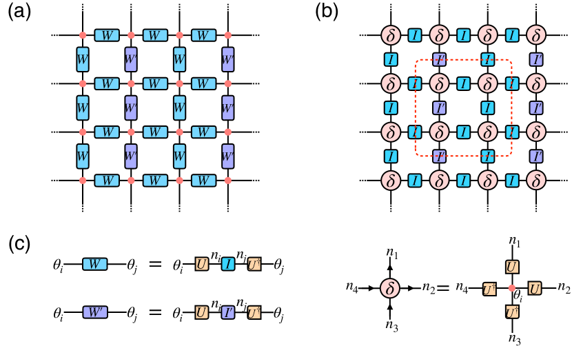
Figure 2: (a) Tensor network representation of the partition function with interaction matrices on the links accounting for the Boltzmann weight. (b) Tensor network representation of the partition function defined on the original lattice. The translation invariant cluster is circled by the red dotted line. (c) The eigenvalue decompositions of the interaction matrices and the construction of delta tensor.

The real challenge comes from the construction of the local tensors under the ground-state local rules. For the classical XY model, to build the translation invariant local tensors, we can simply split the diagonal spectrum $I_{n}$ tensors and take a contraction of four $\sqrt{I_{n}}$ tensors connected to the $\delta$ tensors at the same siteYu et al. (2014); Vanderstraeten et al. (2019b). For the FFXY model with a checkerboard-like ground state, the translation invariant unit is a $2\times 2$ plaquette. So it is reasonable to enlarge the unit cell as a cluster consisting of $2\times 2$ tensors, as circled by the red dotted line in Fig. 2(b). However, we find the standard contraction algorithms such as variational uniform matrix product state (VUMPS)Zauner-Stauber et al. (2018); Vanderstraeten et al. (2019a); Nietner et al. (2020) and corner transfer matrix renormalization group (CTMRG)Nishino and Okunishi (1996); Orús and Vidal (2009); Corboz et al. (2014) fail to converge in such a construction of local tensors.

Two important issues are needed to be addressed in this construction. First, from the perspectives of tessellation, the constraints for the phase differences between two nearest neighbor spins are only imposed on the four lattice sites within a cluster. Since two nearest neighbor clusters are separated by an intermediate plaquette, the constraints between the spins across the gutter is lost. Second, the linear transfer matrix composed by an infinite row/column of local tensors under this construction is always non-Hermitian. The key point is that the spectrum tensors $I_{n}^{\prime}$ carry a negative factor $(-1)^{n}$ which can never be divided into two Hermitian adjoint partitions. Moreover, the negative factors cannot be eliminated under any local transforms due to the “odd rules” induced by the gauge fieldVillain (1977a).

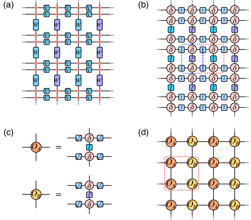
Figure 3: (a) Tensor network representation of the partition function with vertically split $U(1)$ spins. (b) The transformation to discrete degrees of freedom by integrating out $U(1)$ phase variables. (c) The construction of the local $O_{A}$ and $O_{B}$ tensors. (d) The appropriate construction of the tensor network for the partition function encoding the constraints.

In order to solve these problems, we propose a new construction method based on the split of $U(1)$ spins on the lattice site. As shown in Fig. 3(a), each lattice spin is vertically split into two independent spins by using the relation

$$\int d\theta_{i}\,f(\theta_{i})=\iint d\theta_{i}d\theta_{i}^{\prime}\,\delta(\theta_{i}-\theta_{i}^{\prime})f(\theta_{i})$$ (5)

where $f(\theta_{i})$ denotes the rest part of the partition function associated to the lattice site $i$. And the corresponding interaction matrices $W$ are also equally divided into two $V$ tensors as

$$V(\theta_{i},\theta_{j})=\mathrm{e}^{\frac{1}{2}\beta J\cos(\theta_{i}-\theta_{j})}.$$ (6)

Then, we carry out eigenvalue decompositions on the $V$ tensor in the same manner,

$$V(\theta_{i},\theta_{j})=\sum_{n}U_{\theta_{i},n}\,\iota_{n}(\beta J)\,U_{n,\theta_{j}}^{\ast},$$ (7)

where $\iota_{n}(\beta J)=I_{n}(\beta J/2)$. The Dirac delta function connecting two cloned spins can be decomposed by

$$\delta(\theta_{i},\theta_{i}^{\prime})=\frac{1}{2\pi}\sum_{n}U_{\theta_{i},n}\,U_{n,\theta_{i}^{\prime}}^{\ast}.$$ (8)

Again the orthogonality of $U_{n,\theta}$ enables us to integrate out the phase variables at each lattice site, and the enlarged tensor network is displayed in Fig. 3(b).

Now, we are able to walk around the obstacles by an appropriate construction of the network. The minimum building blocks are the local tensors $O_{A}$ and $O_{B}$, whose inner structures are shown in Fig. 3(c). The resulting tensor network $\mathcal{N}$ for the partition function is depicted in Fig. 3(d) as

$$Z=\text{{tTr}}\left(\prod_{O_{A},O_{B}\in\mathcal{N}}O_{A}O_{B}\right),$$ (9)

where “tTr” denotes the tensor contraction over all auxiliary links. Because the expansion coefficients decrease exponentially in $\iota_{n}(x)$ with increasing $n$, an appropriate truncation can be performed on the virtual indices of $O_{A}$ and $O_{B}$ tensors without loss of accuracy. The constraints among four spins within a given plaquette is ensured by choosing a cluster grouping $O_{A}$ and $O_{B}$ tensors. Although the partition function is represented by the row-to-row transfer matrix operator consisting of a single layer of alternating $O_{A}$ and $O_{B}$ tensors, it is only well-defined by even rows due to the non-trivial $2\times 2$ plaquette structure of the checkerboard ground state. Therefore, the unit cluster should be composed by a double stack of $O_{A}$ and $O_{B}$ tensors as grouped by the red dotted line in Fig. 3(d). Ultimately, we obtain the right construction of the tensor network with the linear transfer matrix consisting of the $2\times 2$ clusters. Such a construction gives rise to the right partition function by realizing that (i) all the constraints are preserved within the transfer matrix while the spins across the gutter between two transfer matrices are indeed the same spin, (ii) the transfer matrix is Hermitian as the splitting of the $I^{\prime}$ tensors is no longer needed.

Apart from the representation in the original lattice, there is another approach to express the partition function as a tensor network on the dual lattice with automatically encoded local constraints. For a model with discrete degrees of freedom, the dual construction can always be performed by splitting of the model Hamiltonian on a shared bond, and the local tensors are defined on the plaquette centers by grouping the split bonds which are connected by Kronecker delta functions. However, this strategy cannot be simply extended for the case of the continuous degrees of freedom. When we split each bond around the plaquette, there will be integrals of loops of Dirac delta functions, which is not well-defined mathematically. That is why we can only split the $W$ tensors in Fig. 2(a) horizontally. We also notice that the duality transformation of the FFXY model onto the dual height model cannot give the appropriate partition function, as a finite truncation on the height can mess up the Boltzmann weights. Therefore, the construction of the tensor network in the dual space remains an open problem.

III.2 Multisite VUMPS algorithm

Within the framework of tensor network, the fundamental object for the calculation of the partition function is the transfer operator composed of two infinite rows of alternating $O_{A}$ and $O_{B}$ tensors

$$\mathcal{T}(\beta)=\mathrm{{tTr}\,\left[\begin{array}[]{c}{{\cdots O_{A}O_{B}O_{A}O_{B}\cdots}}\\ {{\cdots O_{A}^{\prime}O_{B}^{\prime}O_{A}^{\prime}O_{B}^{\prime}\cdots}}\end{array}\right],}$$ (10)

where the prime symbols are just a mark to distinguish the second row from the first row. This operator can be regarded as the matrix product operator (MPO) for the 1D quantum spin chain, whose logarithmic form can be mapped to a 1D quantum system with complicated spin-spin interactions. In this way, the correspondence between the finite temperature 2D statistical model and the 1D quantum model at zero temperature is established.

As sketched in Fig. 4(a), the value for the partition function is determined by the dominant eigenvalues of the transfer matrix

$$\mathcal{T}(\beta)|\Psi(A,B)\rangle=\Lambda_{\max}|\Psi(A,B)\rangle,$$ (11)

where $|\Psi(A,B)\rangle$ is the leading eigenvector represented by matrix product states (MPS) made up of two-site unit cell of local $A$ and $B$ tensorsZauner-Stauber et al. (2018). This fixed-point equation can be accurately solved by the multiple lattice-site VUMPS algorithmNietner et al. (2020), which provides an efficient variational scheme to approximate the largest eigenvector $|\Psi(A,B)\rangle$. The precision of this approximation is controlled by the auxiliary bond dimension $D$ of local $A$ and $B$ tensors. Instead of grouping the local tensors of a cluster into a trivial unit cell at the cost of growing the bond dimension of the MPO exponentially, the multisite VUMPS algorithm brings about a significant speed-up with a computational complexity only scaling linearly with the size of the multisite cluster.

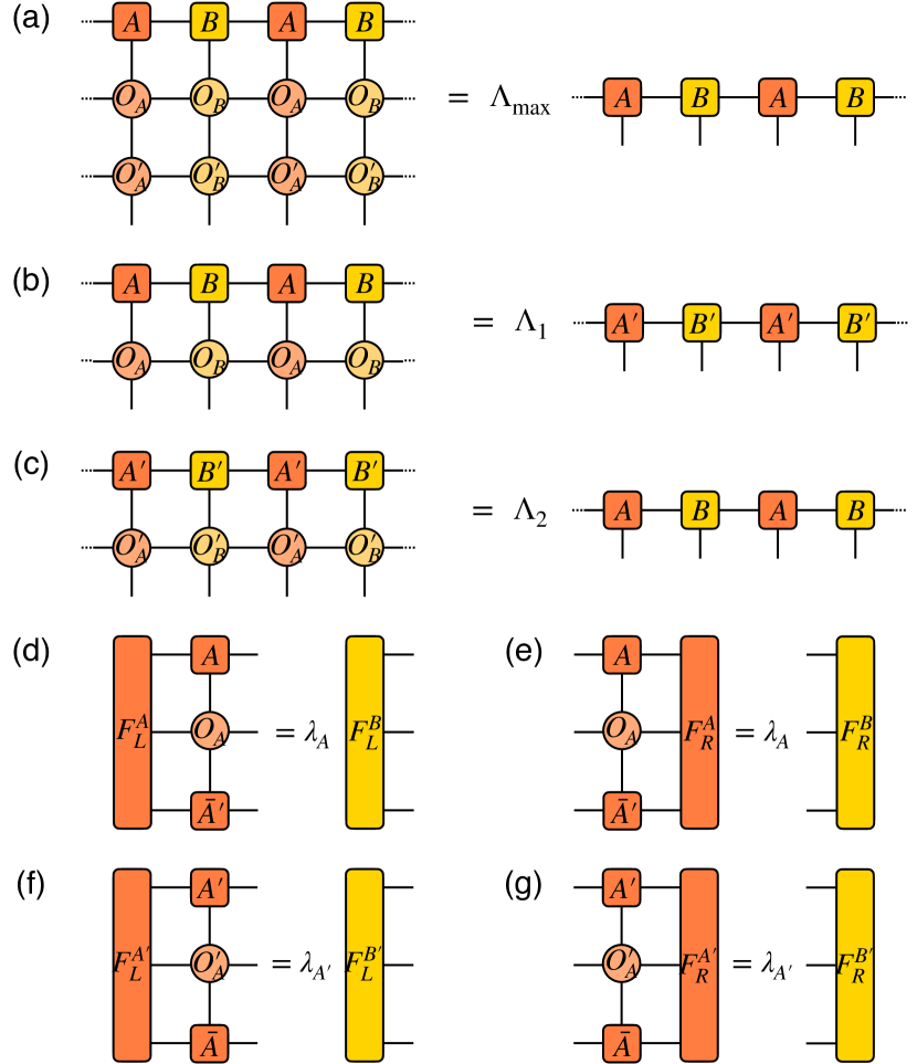
Figure 4: (a) The eigen equation for the fixed-point MPS $|\Psi(A,B)\rangle$ of the transfer operator $\mathcal{T}(\beta)$. (b) and (c) Two smaller linear equations for the first and second row as a decomposition of the fixed-point eigen equation. (d)-(g) Eigen equations for the left and right fixed points of the corresponding channel operators related to $O_{A}$ and $O_{A}^{\prime}$.

The multisite algorithm starts from decomposing the big eigen equation into two smaller linear equations as shown in Fig. 4(b) and (c):

$$T_{1}(\beta)|\Psi(A,B)\rangle =\Lambda_{1}\Psi(A^{\prime},B^{\prime})\rangle,$$

$$T_{2}(\beta)|\Psi(A^{\prime},B^{\prime})\rangle =\Lambda_{2}|\Psi(A,B)\rangle,$$ (12)

where $T_{1}(\beta)$ and $T_{2}(\beta)$ correspond to the first and second row of the blocked transfer matrix $\mathcal{T}(\beta)$, whose eigenvalue is a combination as $\Lambda_{\max}=\Lambda_{1}\Lambda_{2}$. In practice, the linear equations are transformed into a set of optimization problems

$$\Lambda_{1} =\max_{A,B,A^{\prime},B^{\prime}}\langle\Psi(A,B)|T_{1}(\beta)|\Psi(\bar{A^{\prime}},\bar{B^{\prime}})\rangle,$$

$$\Lambda_{2} =\max_{A,B,A^{\prime},B^{\prime}}\langle\Psi(A^{\prime},B^{\prime})|T_{1}(\beta)|\Psi(\bar{A},\bar{B})\rangle,$$

which can be solved efficiently by applying the VUMPS algorithmZauner-Stauber et al. (2018); Vanderstraeten et al. (2019a) based on the tangent space projections in iteration.

One of the key steps in the iteration of VUMPS method is the calculation of the leading left- and right-eigenvectors of the channel operators. The channel operators have a sandwich structure composed of two local tensors of fixed point MPS and the middle four-leg local tensor. The channel operator related to $A$ tensor is defined by

$$\mathbb{T}_{X}^{A}=\sum_{i,j}\bar{A}^{i}\otimes X^{i,j}\otimes\bar{A^{\prime}}^{j},$$ (13)

and other channel operators are defined in the same way. For the $2\times 2$ unit cell, there are four set of eigen equations for the left- and right-fixed points of the corresponding channel operators. Fig. 4(d)-(g) displays the eigen equations related to $O_{A}$ and $O_{A^{\prime}}$

$$\left\langle F_{L}^{A}\right|\mathbb{T}_{O_{A}}^{A}=\lambda_{A}\left\langle F_{L}^{B}\right|,\ \ \mathbb{T}_{O_{A}}^{A}\left|F_{R}^{A}\right\rangle=\lambda_{A}\left|F_{R}^{B}\right\rangle,$$

$$\langle F_{L}^{A^{\prime}}|\mathbb{T}_{O_{A}^{\prime}}^{A^{\prime}}=\lambda_{A^{\prime}}\langle F_{L}^{B^{\prime}}|,\ \ \mathbb{T}_{O_{A}^{\prime}}^{A^{\prime}}|F_{R}^{A^{\prime}}\rangle=\lambda_{A^{\prime}}|F_{R}^{B^{\prime}}\rangle,$$ (14)

and the same method are applied to $O_{B}$ and $O_{B^{\prime}}$. The above equations only map two fixed points in the same row to each other without directly giving an eigenvalue problem. In the same spirit as the solvers for fixed-point MPS, these equations are iteratively applied until a given convergence criterion is reached.

III.3 Calculations of the physical quantities

Once the fixed point MPS is achieved, various physical quantities can be accurately calculated in the tensor-network language. The entanglement properties can be detected via the Schmidt decomposition of $|\Psi(A,B)\rangle$ which bipartites the relevant 1D quantum state of the MPO, and the entanglement entropyVidal et al. (2003) is determined directly from the singular values $s_{\alpha}$ as

$$S_{E}=-\sum_{\alpha=1}^{D}s_{\alpha}^{2}\ln s_{\alpha}^{2},$$ (15)

in correspondence to the quantum entanglement measure for a many-body quantum system.

Local observable can be evaluated by inserting the corresponding impurity tensors into the original tensor network for the partition function. We can squeeze the whole network into an infinite chain of channel operators by sequentially pulling the MPS fixed points through the network from top and bottom. Then a further contraction is performed by the left and right fixed points of the channel operators. For instance, the expectation value of the local chirality at a plaquette $p$ is defined as

$$\tau_{p}=\frac{1}{2\sqrt{2}}\sum_{\langle i,j\rangle\in\Box_{p}}\left\langle\sin(\theta_{i}-\theta_{j}+A_{ij})\right\rangle,$$ (16)

where the sum runs over the four bonds around the plaquette anti-clockwise, corresponding to four pairs of nearest-neighbor two-angle observable. For the FFXY model with checkerboard like order of the chirality, it is necessary to pick out a unit cell of $2\times 2$ plaquette as shown in Fig. 5(a), where the sub-plaquettes are labeled with $a$, $b$, $c$ and $d$. The number of two-angle observable needed to evaluate the local chirality of the sub-lattices can be reduced from twelve to eight due to the transitional symmetry of the unit cell. It is easy to check the identities between the observable at boundaries like

$$\langle\mathrm{e}^{i(\theta_{1,1}-\theta_{1,2})}\rangle = \langle\mathrm{e}^{i(\theta_{3,1}-\theta_{3,2})}\rangle$$ (17)

$$= \frac{1}{Z}\prod_{i}\frac{d\theta_{i}}{2\pi}\mathrm{e}^{-\beta E(\{\theta_{i}\})}\mathrm{e}^{i\theta_{1,1}}\mathrm{e}^{-i\theta_{1,2}},$$

where $E(\{\theta_{i}\})$ is the energy for a given spin configuration. Compared to the orthogonal relation of (4), $\mathrm{e}^{i\theta_{1,1}}$ and $\mathrm{e}^{-i\theta_{1,2}}$ in the second row simply change the corresponding delta tensors in the original tensor network for the partition function in Fig. 3(b) into

$$\delta_{+}=\delta_{n_{1}+n_{2}+1}^{n_{3}+n_{4}},\quad\delta_{-}=\delta_{n_{1}+n_{2}}^{n_{3}+n_{4}+1},$$ (18)

which introduce the impurity tensors $M^{+}$ and $N^{-}$ containing these imbalanced delta tensors into the tensor network of Fig. 3(d). The structure of the impurity tensors are displayed in Fig. 5(b) as $M_{\varepsilon}^{\upsilon}$ and $N_{\varepsilon}^{\upsilon}$ in replacement of $O_{A}$ and $O_{B}$, respectively, where $\varepsilon,\upsilon=\pm$ are in consistent with $\delta_{\pm}$. Here the superscript and subscript in $M$ and $N$ are omitted when there is a normal delta tensor defined by (4). With the help of the fixed-points of the channel operators, it is straightforward to get the two-angle observable sharing the vertical bonds:

$$\langle\mathrm{e}^{i(\theta_{2,1}-\theta_{1,1})}\rangle=\langle F_{L}^{A}|\mathbb{T}_{M_{+}^{-}}^{A}|F_{R}^{A}\rangle,$$ (19)

and those living on the horizontal bonds:

$$\langle\mathrm{e}^{i(\theta_{1,1}-\theta_{1,2})}\rangle=\langle F_{L}^{A}|\mathbb{T}_{M^{+}}^{A}\mathbb{T}_{N^{-}}^{B}|F_{R}^{B}\rangle,$$ (20)

as graphically depicted in Fig. 5(c) and (d). Finally, we deduce the local chiralities at four sub-plaquettes from the imaginary part of theses two-angle observable and the internal energy per site can be obtained readily from the real part as

$$u=-\frac{J}{2}\sum_{\langle i,j\rangle\in\Box}\left\langle\cos(\theta_{i}-\theta_{j}+A_{ij})\right\rangle.$$ (21)

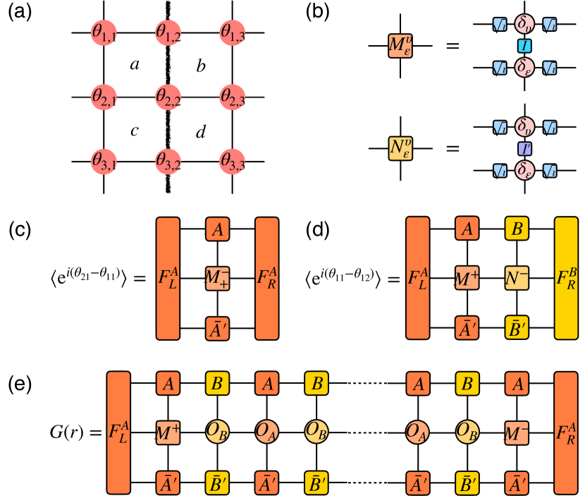
Figure 5: (a) A unit cell of $2\times 2$ plaquettes with $9$ spins at vertices. (b) The construction of the impurity tensors from imbalanced delta tensors. (c) and (d) Evaluations of the nearest-neighbor two-angle observables living on the vertical and horizontal bonds. (e) Two-point correlation function represented by contracting a sequence of channel operators.

Moreover, the two-point correlation function between local observable is defined by $G(r)=\langle h(\theta_{j})h(\theta_{j+r})\rangle$, which can be evaluated by inserting two local impurity tensors into the original tensor network. The corresponding impurity tensors are constructed in the same way by altering the Kronecker delta tensors:

$$\delta_{n_{1},n_{2}}^{n_{3},n_{4}}\rightarrow\int\frac{d\theta}{2\pi}\,\mathrm{e}^{i(n_{1}+n_{2}-n_{3}-n_{4})}h(\theta).$$ (22)

For the spin-spin correlation function, as shown in Fig. 5(e), the evaluation of $G(r)=\langle\mathrm{e}^{i(\theta_{j}-\theta_{j+r})}\rangle$ is reduced to a trace of a row of channel operators containing two impurity tensors $M^{+}$ and $N^{-}$

$$G(r)=\langle F_{L}^{A}|\mathbb{T}_{M^{+}}^{A}\underbrace{\mathbb{T}_{O}^{B}\mathbb{T}_{O}^{A}\mathbb{T}_{O}^{B}\cdots\mathbb{T}_{O}^{A}\mathbb{T}_{O}^{B}}_{r-1}\mathbb{T}_{M^{-}}^{A}|F_{R}^{A}\rangle,$$ (23)

where the left and right leading eigenvectors of the channel operators are employed.

IV Numerical Results

Most of the previous studies determine the transition temperature according to some kind of order parameter like the magnetization or Binder cumulant. These order parameters are good criteria to identify the critical temperatures relevant to $U(1)$ or $Z_{2}$ phase transition when several transitions are apart from each other with sufficient distance separation. However, for the case of FFXY model, it is hard to tell apart two kinds of mutually close transitions from these quantities because either the $U(1)$ or $Z_{2}$ transition temperature are obtained from an average with some degrees of uncertainty and the estimated temperatures may mix up with each other. Here, we propose that the entanglement entropy shall shed a new light to overcome the difficulties in deciding whether there are two distinct transitions in the FFXY model. The entanglement entropy of the fixed-point MPS for the 1D quantum transfer operator exhibits singularity at the critical temperatures which offers a sharp criteria to accurately determine all possible phase transitions, especially for systems possessing $U(1)\times Z_{2}$ symmetrySong and Zhang (2021a, b).

As shown in Fig. 6, the entanglement entropy $S_{E}$ develops two sharp singularity at two critical temperatures $T_{c1}$ and $T_{c2}$, which strongly indicates the existence of two phase transitions at two different temperatures. As the singularity positions vary with the MPS bond dimension $D$, the critical temperatures $T_{c1}$ and $T_{c2}$ can be determined precisely by extrapolating the bond dimension $D$ to infinite. Moreover, we find that the critical temperatures $T_{c1}$ and $T_{c2}$ exhibit different scaling behavior in the linear extrapolation, implying that that the two phase transitions belong to different kinds of universality class. The inset of Fig. 6 displays how the critical temperatures, $T_{c1}$ and $T_{c2}$, vary with the MPS bond dimensions. The lower transition temperature $T_{c1}$ varies linearly on the inverse square of the logarithm of the bond dimension, while the higher transition temperature $T_{c2}$ has a linear variance with the inverse bond dimension. From the linear extrapolation, the critical temperatures are estimated to be $T_{c1}\simeq 0.4459$ and $T_{c2}\simeq 0.4532$, which agrees well with the previous Monte Carlo simulationsOlsson (1995); Okumura et al. (2011).

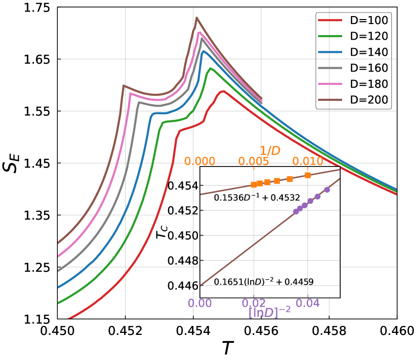
Figure 6: The entanglement entropy as a function of temperature develops two singularities at $T_{c1}$ and $T_{c2}$ indicating two phase transitions for different MPS bond dimensions. Inset: The singularity temperatures $T_{c1}$ and $T_{c2}$ of the entanglement entropy fitted for MPS bond dimensions from $100$ to $200$ with an interval of $20$. The lower transition temperature $T_{c1}$ varies linearly on $(\ln D)^{-2}$, while the higher transition temperature $T_{c2}$ has a linear variance with $1/D$.

Actually, the different scaling behavior stems from the different critical behavior of the BKT and 2D Ising transitions. The BKT transition for $T>T_{C}$ is characterized by the exponentially diverging correlation length

$$\xi_{BKT}(T)\propto\exp(b/\sqrt{T-T_{C}}),$$

while the 2D Ising transition is featured by

$$\xi_{Ising}(T)\propto 1/|T-T_{C}|.$$

Since the bond dimensions of the fixed-point MPS can be regarded as a finite cutoff on the diverging correlation length, it is reasonable to use the $(\ln D)^{-2}$ and the $1/D$ scaling for the extrapolation of the critical temperatures $T_{c1}$ and $T_{c2}$, respectively. Besides, the separation between $T_{c1}$ and $T_{c2}$ gets larger as the bond dimension increases, which indicates that large bond dimensions are necessary to clarify the nature of the transitions.

In order to gain insight into the essential physics of different phase transitions, we investigate the thermodynamic properties. We begin with the specific heat which can be derived directly from $C_{V}=du/dT$, where $u$ is the internal energy obtained by the contraction of the tensor network with the nearest-neighbor impurity tensors as introduced in (21). As shown in Fig. 7(a), the specific heat exhibits a logarithmic divergence at $T>T_{c2}$ but a small bump around $T_{c1}$. The logarithmic specific heat at the higher temperature side indicates the occurrence of a second-order phase transition such as the 2D Ising phase transition, while the small bump at the lower temperature can be regarded as a higher order continuous phase transition like the BKT transition. The specific heat curve is inadequate for a logarithmic fitting at the lower temperature side of $T_{c2}$ because two different transitions are still closed to each other.

It is natural to expect that the logarithmic peak of the specific heat is related to the breaking of the chiral order as the FFXY has a checkerboard ground state with $Z_{2}$ symmetry. We thus check this long-range ordering of the local chirality $\tau$ at the sub-plaquettes defined by (16) within a transition invariant unit cell depicted in Fig. 5(a). As shown in Fig. 7(b), the expectation values of the local chirality are finite below $T_{c2}$, indicating the formation of the long-range $Z_{2}$ order. In addition, we find a perfect agreement for the four chiralities as $\tau_{a}=-\tau_{b}=-\tau_{c}=\tau_{d}$, which is a clear evidence for the emergence of the checkerboard pattern through the phase transition at $T_{c2}$. The checkerboard like order of the chirality can be characterized by a staggered magnetization defined as

$$m=\frac{1}{N}\sum_{\Box_{p}}(-1)^{x_{p}+y_{p}}\tau_{p},$$ (24)

where $\tau_{p}$ is the local chirality at the center of the plaquette located at position $(x_{p},y_{p})$. As the temperature approaching $T_{c2}$ from below, we find that $m$ vanishes continuously as $m\sim t^{\beta}$ with $t\equiv(T_{c2}-T)/T_{c2}$, where $\beta\simeq 1/8$ is the critical exponents characteristic of the 2D Ising model. The linear fitting of $\ln m\propto\beta\ln t$ is depicted in the inset of Fig. 7(b). Therefore, there is a convincing evidence that the transition at $T_{c2}$ belongs to the 2D Ising universality class.

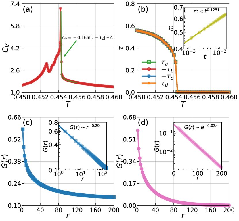
Figure 7: (a) The specific heat develops a small bump and sharp peak at $T_{c1}$ and $T_{c2}$, respectively. The green line is a fitting curve of the logarithmic divergence for $T>T_{c2}$. (b) The establishment of the checkerboard like pattern of local chiralities below $T_{c2}$. Inset is the fitting of the critical exponent of the staggered magnetization. (c) The spin-spin correlation function displays power law behavior at $T=0.450$ below $T_{c1}$. (d) The spin-spin correlation function decays exponentially at $T=0.454$ at the intermediate temperature between $T_{c1}$ and $T_{c2}$.

From the analysis of the specific heat, we are aware of the transition at $T_{c1}$ related to a spin ordering, which is completely different from the second order phase transitions. To further explore the nature of the phase transition, we calculate the spin-spin correlation function

$$G(r)=\langle\psi^{\ast}(r)\psi(0)\rangle\propto\langle\cos(\theta_{0}-\theta_{r})\rangle$$

within the tensor network framework by (23). As displayed in Fig. 7(c), the spin-spin correlation function exhibits an algebraic behavior below $T_{c1}$, implying the vortex-antivortex bindings in the spin configuration. However, for the temperature above $T_{c1}$, $G(r)$ decays exponentially, indicating the destruction of phase coherence between vortex pairs. Fig. 7(d) shows the exponential behavior of $G(r)$ at an intermediate temperature between $T_{c1}$ and $T_{c2}$. Hence, the change in the behavior of the correlation function at $T_{c1}$ turns out to be in the universality class of the BKT transition.

Finally, the whole phase structure is summarized in Fig. 1(b). The FFXY model has two very close but separate phase transitions, with transition temperature $T_{BKT}<T_{Ising}$. The transition at $T_{Ising}$ belongs to the usual 2D Ising universality class, while the transition at $T_{BKT}$ belongs to the BKT universality class. As the system cools down, the $Z_{2}$ symmetry is first broken at $T_{Ising}$ characterized by the formation of checkerboard like long-range order of chiralities, and then the BKT transition occurs at a lower temperature $T_{BKT}$ featured by the algebraic correlation between vortex-antivortex pairs.

V Conclusion

We have proposed a general framework to solve the 2D FFXY model. The important aspect is to encode the ground-state local rules induced by frustrations into the local tensors of the partition function. Then the partition function is written in terms of a product of 1D transfer matrix operator, whose eigen-equation is solved by an algorithm of matrix product states rigorously. The singularity of the entanglement entropy for this 1D quantum analogue provides a stringent criterion to determine various phase transitions without identifying any order parameter a prior. Certainly the present methods provide a promising route to solve other frustrated lattice models with continuous degrees of freedom in 2D.

The main result of our tensor network theory is that, higher than the BKT phase transition, a chiral ordered phase with spontaneously broken $Z_{2}$ symmetry has been confirmed, where the spin-spin phase coherence is absent but the phase differences of the spins on two nearest neighbor sites have a nontrivial value different from $0$ or $\pi$. In contrast to the conventional situations where the Ising transition happens at a lower temperature below the BKT transition, the ordering of the spins in the FFXY model is nontrivial. It is highly interesting that the chiral ordered intermediate phase may be related to some unconventional superconductivity in the absence of condensed Cooper pairs.

Furthemore, another phase transition associated with the unbinding of kink pairs on domain walls in the FFXY modelKorshunov (2002) was proposed to support the existence of two separate bulk transitions $T_{BKT}<T_{Ising}$, which happens at a lower temperature $T_{kink}<T_{BKT}$. The kinks at the corners of domain walls behave as fractional vortices with the topological charge $\pm\frac{1}{4}$. However, the verification of such transition is only realized under a special boundary condition where an infinite domain wall is ensuredOlsson and Teitel (2005). We believe that our tensor network approach may provide a promising way for further detailed investigations of such kink-antikink unbinding transition.

Acknowledgments The authors are very grateful to Qi Zhang for his stimulating discussions. The research is supported by the National Key Research and Development Program of MOST of China (2017YFA0302902).

References

- Berezinsky (1971) V. Berezinsky, Sov. Phys. JETP 32, 493 (1971).
- Kosterlitz and Thouless (1973) J. M. Kosterlitz and D. J. Thouless, 6, 1181 (1973), URL https://doi.org/10.1088/0022-3719/6/7/010.
- Resnick et al. (1981) D. J. Resnick, J. C. Garland, J. T. Boyd, S. Shoemaker, and R. S. Newrock, Phys. Rev. Lett. 47, 1542 (1981), URL https://link.aps.org/doi/10.1103/PhysRevLett.47.1542.
- Abraham et al. (1982) D. W. Abraham, C. J. Lobb, M. Tinkham, and T. M. Klapwijk, Phys. Rev. B 26, 5268 (1982), URL https://link.aps.org/doi/10.1103/PhysRevB.26.5268.
- van Wees et al. (1987) B. J. van Wees, H. S. J. van der Zant, and J. E. Mooij, Phys. Rev. B 35, 7291 (1987), URL https://link.aps.org/doi/10.1103/PhysRevB.35.7291.
- Fazio and van der Zant (2001) R. Fazio and H. van der Zant, Physics Reports 355, 235 (2001), ISSN 0370-1573, URL https://www.sciencedirect.com/science/article/pii/S0370157301000229.
- Newrock et al. (2000) R. Newrock, C. Lobb, U. Geigenmüller, and M. Octavio, in The Two-Dimensional Physics of Josephson Junction Arrays, edited by H. Ehrenreich and F. Spaepen (Academic Press, 2000), vol. 54 of Solid State Physics, pp. 263–512, URL https://www.sciencedirect.com/science/article/pii/S0081194708602507.
- Cosmic et al. (2020a) R. Cosmic, K. Kawabata, Y. Ashida, H. Ikegami, S. Furukawa, P. Patil, J. M. Taylor, and Y. Nakamura, Phys. Rev. B 102, 094509 (2020a), URL https://link.aps.org/doi/10.1103/PhysRevB.102.094509.
- van der Zant et al. (1991) H. S. J. van der Zant, H. A. Rijken, and J. E. Mooij, Journal of Low Temperature Physics 82, 67 (1991), URL https://doi.org/10.1007/BF00681552.
- Ling et al. (1996) X. S. Ling, H. J. Lezec, M. J. Higgins, J. S. Tsai, J. Fujita, H. Numata, Y. Nakamura, Y. Ochiai, C. Tang, P. M. Chaikin, et al., Phys. Rev. Lett. 76, 2989 (1996), URL https://link.aps.org/doi/10.1103/PhysRevLett.76.2989.
- Martinoli and Leemann (2000) P. Martinoli and C. Leemann, Journal of Low Temperature Physics 118, 699 (2000), URL https://doi.org/10.1023/A:1004651730459.
- Cosmic et al. (2020b) R. Cosmic, K. Kawabata, Y. Ashida, H. Ikegami, S. Furukawa, P. Patil, J. M. Taylor, and Y. Nakamura, Phys. Rev. B 102, 094509 (2020b), URL https://link.aps.org/doi/10.1103/PhysRevB.102.094509.
- Villain (1977a) J. Villain, Journal of Physics C: Solid State Physics 10, 1717 (1977a), URL https://doi.org/10.1088/0022-3719/10/10/014.
- Villain (1977b) J. Villain, Journal of Physics C: Solid State Physics 10, 4793 (1977b), URL https://doi.org/10.1088/0022-3719/10/23/013.
- Teitel and Jayaprakash (1983) S. Teitel and C. Jayaprakash, Phys. Rev. B 27, 598 (1983), URL https://link.aps.org/doi/10.1103/PhysRevB.27.598.
- Thijssen and Knops (1990) J. M. Thijssen and H. J. F. Knops, Phys. Rev. B 42, 2438 (1990), URL https://link.aps.org/doi/10.1103/PhysRevB.42.2438.
- Ramirez-Santiago and José (1992) G. Ramirez-Santiago and J. V. José, Phys. Rev. Lett. 68, 1224 (1992), URL https://link.aps.org/doi/10.1103/PhysRevLett.68.1224.
- Granato and Nightingale (1993) E. Granato and M. P. Nightingale, Phys. Rev. B 48, 7438 (1993), URL https://link.aps.org/doi/10.1103/PhysRevB.48.7438.
- Lee (1994) J.-R. Lee, Phys. Rev. B 49, 3317 (1994), URL https://link.aps.org/doi/10.1103/PhysRevB.49.3317.
- Lee and Lee (1994) S. Lee and K.-C. Lee, Phys. Rev. B 49, 15184 (1994), URL https://link.aps.org/doi/10.1103/PhysRevB.49.15184.
- Ramirez-Santiago and José (1994) G. Ramirez-Santiago and J. V. José, Phys. Rev. B 49, 9567 (1994), URL https://link.aps.org/doi/10.1103/PhysRevB.49.9567.
- Olsson (1995) P. Olsson, Phys. Rev. Lett. 75, 2758 (1995), URL https://link.aps.org/doi/10.1103/PhysRevLett.75.2758.
- Cataudella and Nicodemi (1996) V. Cataudella and M. Nicodemi, Physica A: Statistical Mechanics and its Applications 233, 293 (1996), ISSN 0378-4371, URL https://www.sciencedirect.com/science/article/pii/S0378437196002105.
- Olsson (1997) P. Olsson, Phys. Rev. B 55, 3585 (1997), URL https://link.aps.org/doi/10.1103/PhysRevB.55.3585.
- Boubcheur and Diep (1998) E. H. Boubcheur and H. T. Diep, Phys. Rev. B 58, 5163 (1998), URL https://link.aps.org/doi/10.1103/PhysRevB.58.5163.
- Hasenbusch et al. (2005) M. Hasenbusch, A. Pelissetto, and E. Vicari, 2005, P12002 (2005), URL https://doi.org/10.1088/1742-5468/2005/12/p12002.
- Okumura et al. (2011) S. Okumura, H. Yoshino, and H. Kawamura, Phys. Rev. B 83, 094429 (2011), URL https://link.aps.org/doi/10.1103/PhysRevB.83.094429.
- Nussinov (2014) Z. Nussinov, Journal of Statistical Mechanics: Theory and Experiment 2014, P02012 (2014), URL https://doi.org/10.1088/1742-5468/2014/02/p02012.
- Lima et al. (2019) A. B. Lima, L. A. S. Mól, and B. V. Costa, Journal of Statistical Physics 175, 960 (2019), URL https://doi.org/10.1007/s10955-019-02271-x.
- Miyashita and Shiba (1984) S. Miyashita and H. Shiba, Journal of the Physical Society of Japan 53, 1145 (1984), eprint https://doi.org/10.1143/JPSJ.53.1145, URL https://doi.org/10.1143/JPSJ.53.1145.
- Shih and Stroud (1984) W. Y. Shih and D. Stroud, Phys. Rev. B 30, 6774 (1984), URL https://link.aps.org/doi/10.1103/PhysRevB.30.6774.
- Lee et al. (1984) D. H. Lee, J. D. Joannopoulos, J. W. Negele, and D. P. Landau, Phys. Rev. Lett. 52, 433 (1984), URL https://link.aps.org/doi/10.1103/PhysRevLett.52.433.
- Lee et al. (1986) D. H. Lee, J. D. Joannopoulos, J. W. Negele, and D. P. Landau, Phys. Rev. B 33, 450 (1986), URL https://link.aps.org/doi/10.1103/PhysRevB.33.450.
- Korshunov and Uimin (1986) S. E. Korshunov and G. V. Uimin, Journal of Statistical Physics 43, 1 (1986), URL https://doi.org/10.1007/BF01010569.
- Van Himbergen (1986) J. E. Van Himbergen, Phys. Rev. B 33, 7857 (1986), URL https://link.aps.org/doi/10.1103/PhysRevB.33.7857.
- Xu and Southern (1996) H.-J. Xu and B. W. Southern, 29, L133 (1996), URL https://doi.org/10.1088/0305-4470/29/5/009.
- Lee and Lee (1998) S. Lee and K.-C. Lee, Phys. Rev. B 57, 8472 (1998), URL https://link.aps.org/doi/10.1103/PhysRevB.57.8472.
- Capriotti et al. (1998) L. Capriotti, R. Vaia, A. Cuccoli, and V. Tognetti, Phys. Rev. B 58, 273 (1998), URL https://link.aps.org/doi/10.1103/PhysRevB.58.273.
- Wolff (1989) U. Wolff, Phys. Rev. Lett. 62, 361 (1989), URL https://link.aps.org/doi/10.1103/PhysRevLett.62.361.
- Verstraete et al. (2008) F. Verstraete, V. Murg, and J. Cirac, Advances in Physics 57, 143 (2008), eprint https://doi.org/10.1080/14789940801912366, URL https://doi.org/10.1080/14789940801912366.
- Orús (2014) R. Orús, Annals of Physics 349, 117 (2014), ISSN 0003-4916, URL https://www.sciencedirect.com/science/article/pii/S0003491614001596.
- Vanderstraeten et al. (2018) L. Vanderstraeten, B. Vanhecke, and F. Verstraete, Phys. Rev. E 98, 042145 (2018), URL https://link.aps.org/doi/10.1103/PhysRevE.98.042145.
- Vanhecke et al. (2021) B. Vanhecke, J. Colbois, L. Vanderstraeten, F. Verstraete, and F. Mila, Phys. Rev. Research 3, 013041 (2021), URL https://link.aps.org/doi/10.1103/PhysRevResearch.3.013041.
- Nietner et al. (2020) A. Nietner, B. Vanhecke, F. Verstraete, J. Eisert, and L. Vanderstraeten, Quantum 4, 328 (2020), ISSN 2521-327X, URL https://doi.org/10.22331/q-2020-09-21-328.
- Zauner-Stauber et al. (2018) V. Zauner-Stauber, L. Vanderstraeten, M. T. Fishman, F. Verstraete, and J. Haegeman, Phys. Rev. B 97, 045145 (2018), URL https://link.aps.org/doi/10.1103/PhysRevB.97.045145.
- Vanderstraeten et al. (2019a) L. Vanderstraeten, J. Haegeman, and F. Verstraete, SciPost Phys. Lect. Notes p. 7 (2019a), URL https://scipost.org/10.21468/SciPostPhysLectNotes.7.
- Haegeman and Verstraete (2017) J. Haegeman and F. Verstraete, Annual Review of Condensed Matter Physics 8, 355 (2017), eprint https://doi.org/10.1146/annurev-conmatphys-031016-025507, URL https://doi.org/10.1146/annurev-conmatphys-031016-025507.
- Yu et al. (2014) J. F. Yu, Z. Y. Xie, Y. Meurice, Y. Liu, A. Denbleyker, H. Zou, M. P. Qin, J. Chen, and T. Xiang, Phys. Rev. E 89, 013308 (2014), URL https://link.aps.org/doi/10.1103/PhysRevE.89.013308.
- Vanderstraeten et al. (2019b) L. Vanderstraeten, B. Vanhecke, A. M. Läuchli, and F. Verstraete, Phys. Rev. E 100, 062136 (2019b), URL https://link.aps.org/doi/10.1103/PhysRevE.100.062136.
- Song and Zhang (2021a) F.-F. Song and G.-M. Zhang, Phys. Rev. B 103, 024518 (2021a), URL https://link.aps.org/doi/10.1103/PhysRevB.103.024518.
- Nishino and Okunishi (1996) T. Nishino and K. Okunishi, Journal of the Physical Society of Japan 65, 891 (1996), eprint https://doi.org/10.1143/JPSJ.65.891, URL https://doi.org/10.1143/JPSJ.65.891.
- Orús and Vidal (2009) R. Orús and G. Vidal, Phys. Rev. B 80, 094403 (2009), URL https://link.aps.org/doi/10.1103/PhysRevB.80.094403.
- Corboz et al. (2014) P. Corboz, T. M. Rice, and M. Troyer, Phys. Rev. Lett. 113, 046402 (2014), URL https://link.aps.org/doi/10.1103/PhysRevLett.113.046402.
- Vidal et al. (2003) G. Vidal, J. I. Latorre, E. Rico, and A. Kitaev, Phys. Rev. Lett. 90, 227902 (2003), URL https://link.aps.org/doi/10.1103/PhysRevLett.90.227902.
- Song and Zhang (2021b) F.-F. Song and G.-M. Zhang, Phase coherence of pairs of cooper pairs as quasi-long-range order of half-vortex pairs in a two-dimensional bilayer system (2021b), eprint arXiv:2105.05411.
- Korshunov (2002) S. E. Korshunov, Phys. Rev. Lett. 88, 167007 (2002), URL https://link.aps.org/doi/10.1103/PhysRevLett.88.167007.
- Olsson and Teitel (2005) P. Olsson and S. Teitel, Phys. Rev. B 71, 104423 (2005), URL https://link.aps.org/doi/10.1103/PhysRevB.71.104423.