Horospherical random graphs and lockdown strategies

Abstract.

Expanders are sparse graph that are strongly connected, where connectivity is quantified using eigenvalues of the adjacency matrix, and sparsity in terms of vertex valency. We give a model of random graphs and study their connectivity and sparsity. This model is a particular case of soft geometric random graphs, and allows to construct sparse graphs with good expansion properties, as well as highly clustered ones. On those graphs, we study the speed at which random walks spread in the graph, and visit all vertices. As an illustration, we build a model for mainland France and study the spread of random walks under several types of lockdown. Our experiments show that completely closing medium and long distance travel to slow down the spread of a random walk is more efficient than than local restrictions.

1. Introduction

A common way to model real life phenomena relies on graphs. Here we describe a model where the edges of the graph represent possible routes a contaminant can take to travel, and vertices represents possible sites to infect. A simple random walk represents a theoretical immortal virus strain, and a self-replicating random walk would model an actual spread if one includes a replicating rate. In this work we aim to heuristically illustrate how the underlying geometry of travels plays a crucial role in the spread of a contaminant, as it is closely related to the conductance of the graph, which governs the speed at which a simple random walk visits all the vertices.

Recall from the seminal work of Gromov in [6] that a metric space $(Y,d_{Y})$ is called hyperbolic if loosely speaking every geodesic triangle is uniformly thin regardless of the size of that triangle. Example 1.8.A (b) on page 99 of [6] allows to embed any metric space $(X,d)$ as a horosphere in a hyperbolic metric space: a horosphere is a sphere centered at infinity. The construction consists in adding scaled down layers of the original space thus creating shortcuts in the metric space $(X,d)$, consisting in going up the layers to travel. With this construction, sets that had a small boundary in $X$, have a much larger one when embedded in the hyperbolic space.

We apply this idea to define a model of random graphs, that we call horospherical random graphs, defined by growing layers of graphs and whose limit is a particular case of soft geometric random graphs. Loosely speaking, we start with a metric space, choose vertices using some distribution, and then start at the first level by adding edges between points that are not too distant. Then at the second level, we add edges between points that are further away, etc. After a few levels, those graphs start to exhibit good expanding properties, in the sense that a random walk is very quick to visit all the vertices.

Modelling our random graphs according to the population density of a country (we worked on mainland France for our application in Section 5), the edges represent possible routes that people can take, and hence the paths a virus can use to spread. Different layers of our sequence of graphs illustrate several confinement strategies, giving very different rates at which a random walk visits all the vertices.

Acknowledgements: The authors thank Laurent Saloff-Coste for the reference [10], Goulnara Arzhantseva for discussions and references [12], [8] and [11] as well as Patricia Reynaud-Bouret for interesting conversations and suggesting to look at the Small World features of horospherical graphs. The authors also thank CNRS for making this collaboration materialize.

2. Background on graphs

Recall that a graph $\Gamma$ is the data of a set $V$ of vertices and $E\subseteq V\times V$. Here we will assume our graphs to be undirected simplicial and connected. The adjacency matrix $A=A_{(i,j)}$ of $\Gamma$ is an $n\times n$ matrix, where $n=|V|$ with values 1 when $\{i,j\}\in E$ and 0 otherwise. For an undirected simplicial graph, $A$ is a symmetric matrix with 0’s on the diagonal. We further define the following

1. The degree matrix $D=D_{(i,j)}$ is a diagonal matrix with $D_{(i,i)}$ equals to the degree of the $i$-th vertex: $D_{(i,i)}=\sum_{j}A_{(i,j)}=d_{i}$

2. The normalized adjacency matrix is given by $\overline{A}=AD^{-1}$.

3. The laplacian is given by $L=D-A$.

4. The normalized laplacian is given by $\overline{L}=I-\sqrt{D^{-1}}A\sqrt{D^{-1}}$.

Definition 2.1.

For any two disjoint subsets of vertices $A,B\subseteq V$ , we denote $E(A,B)=E\cap(A\times B\cup B\times A)$, that is the set of edges of $\Gamma$ with one extremity in $A$ and the other in $B$. We denote by $\partial_{E}(A)=E(A,A^{c})$, which are edges of the boundary of $A$. For a subset $A$ in $V$ we define its volume by $\nu(A)=\sum_{x\in A}\nu(x)$, where $\nu(x)=|\{y\in V|\{x,y\}\in E\}|$ is the degree of the vertex $x$. Hence $\nu(\Gamma)=\sum_{x\in V}\nu(x)$ is the total volume of the graph. The conductance of the graph $\Gamma$ is given by

$$\varphi(\Gamma)=\min\{\frac{|\partial_{E}(S)|}{\min\{\nu(S),\nu(V\setminus S)\}}|\emptyset\not=S\subset V\}$$

The conductance is a measure on how well connected the graph $\Gamma$ is. This quantity is difficult to compute, but it is related to the first non-trivial eigenvalue of the normalized laplacian as follows (see for instance Theorem 14.4 of [10] or Fact 6. page 5 of [3])

Theorem 2.2 (Cheeger inequality).

Let $\Gamma$ be a connected graph and let $\lambda_{1}$ be the first non-zero eigenvalue of its normalized laplacian. Then

$$\frac{\lambda_{1}}{2}\leq\varphi(\Gamma)\leq\sqrt{2\lambda_{1}}.$$

Remark 2.3.

Many references (such as for instance [9]) use the expansion constant (or sometimes called Cheeger constant), which is defined by

$$h(\Gamma)=\min\{\frac{|\partial_{E}(A)|}{|A|}\hbox{ such that }\emptyset\not=A\subset V,\ 2|A|\leq|V|\}$$

with the convention that $h(\Gamma)=\infty$ if $\Gamma$ has at most one vertex. The expansion constant measures how difficult it is to separate the graph in two pieces of roughly the same size. Given its definition as a minimum over subsets, the computation of the expansion constant is notoriously difficult to compute. It is also related to the the smallest non-zero eigenvalue of the normalized laplacian, in a similar way as the conductance is.

We will be interested in simple random walks on connected graphs, a walk going to each neighbor with equal probability at each step.

Definition 2.4.

A simple random walk on $\Gamma$ is a sequence $(X_{n})_{n\geq 0}$ of $V$-valued random variables (measurable functions) defined on a common probability space $(\Omega,\Sigma,P)$, with joint distribution satisfying that for any $n\geq 0$, and any vertices $x_{0},\dots,x_{n}$ and $y\in V$, with $\{x_{i},x_{i+1}\}\in E$, then

$$P\{X_{n+1}=y|(X_{n},\dots,X_{0})=(x_{n},\dots,x_{0})\}=P\{X_{n+1}=y|X_{n}=x_{n}\}$$

with

$$P\{X_{n+1}=y|X_{n}=x_{n}\}=\left\{\begin{array}[]{cc}0&\hbox{ if }\{x_{n},y\}\not\in E\\ \frac{1}{|\{x\in V|\{x_{n},x\}\in E\}|}&\hbox{ if }\{x_{n},y\}\in E\end{array}\right.$$

This means that the walk at time $n+1$ doesn’t depend on what happened on the $n-1$ first steps, only on its position in the graph at time $n$.

If the graph is not bipartite, then the walker is, after a time $n$ large enough, as likely to be located at any of the vertices of the graph, independently of the starting point or of the steps taken to get there. We say that the walk converges to the uniform distribution, and $n$, which is the speed at which this convergence occurs, is related to the first eigenvalue $\lambda_{1}$ as follows (see [3] or [10])

$$\left|P(X_{n}=x)-\frac{\nu(x)}{N}\right|\leq\sqrt{\frac{\nu(x)}{v_{-}}}|\lambda_{1}-1|^{n}$$

Intuitively, this means that the walk could be anywhere in the graph, hence has been everywhere in the graph.

Definition 2.5.

The clustering coefficient at a vertex $v_{i}\in V$ is given by

$$C_{i}=2\sum_{j,k}\frac{A_{(i,j)}A_{(j,k)}A_{(k,i)}}{d_{i}(d_{i}-1)}$$

and the average clustering coefficient is the mean value over all vertices, of local clustering coefficients. The clustering coefficient at a vertex $v_{i}$ counts the proportion of closed paths of length 3 at $v_{i}$ among all neighbors of $v_{i}$.

Remark 2.6.

Clustering coefficients are used to give a measure of Small World, those are graphs with a large amount of nodes, that are sparse , with a large average clustering coefficient and small average distances between pairs of points in the graph, see [5] or [14].

3. Description of the probabilistic graph

The general settings for constructing our horospherical random graphs is a particular case of soft random geometric graphs described by Penrose [12], and is described in the following.

Definition 3.1 (Horospherical random graphs).

Suppose that $(X,d)$ is a discrete metric space (for instance obtained from a finite subset of $\mathbb{R}^{n}$ with the induced Euclidean metric from $\mathbb{R}^{n}$). Moreover, suppose that $r_{1}<r_{2}<\ldots\in\mathbb{R}$ is an increasing sequence of real numbers and $\phi=(p_{1},p_{2}\ldots),p_{i}\in[0,1]$ is any sequence of real numbers in the unit interval. This defines a piece-wise constant function $\phi$, taking the value $p_{k}$ in the interval $[r_{k},r_{k+1})$, for any $k\in\mathbb{N}$, called connection function. We define a collection of random graphs $\mathcal{G}=\{\Gamma_{n}\}_{n=1}^{\infty}$ in the following way

• $\Gamma_{1}=(X,E_{1})$ where for all $x\in X$ and for all $x^{\prime}\in X\cap N_{r_{1}}(x)$, the edge $\{x,x^{\prime}\}$ is added to $E_{1}$ with probability $p_{1}$.

• $\Gamma_{n}=(X,E_{n})$ where the edge set is generated randomly as follows:

  • $E_{n-1}\subseteq E_{n}$

  • For all $x\in X$ and for all $x^{\prime}\in X\cap\left(N_{r_{n}}(x)\setminus N_{r_{n-1}}(x)\right)$, the edge $\{x,x^{\prime}\}$ is added to $E_{n}$ with probability $p_{n}$.

The collection $\mathcal{G}$ is what we call horospherical random graph, and for each $i\in{\bf N}$, the graph $\Gamma_{i}$ is the $i$-th layer, or the graph at height $i$. If the connection function $\phi$ is finitely supported, then the collection stabilizes at $\Gamma_{n}$ for $n$ large enough.

Remark 3.2.

If $\Gamma_{1}$ is connected, then $\Gamma_{n}$ is connected for all $n>1$. Moreover, from the definition of conductance it follows that $\varphi(\Gamma_{i})\leq\varphi(\Gamma_{j})$ when $i\leq j$ and according to [4] Theorem 2.1 $\lambda_{k}(\gamma_{j})\geq\lambda_{k}(\Gamma_{i})$ when $j\geq i$, with equality when the eigenvalues are 0. Our goal will be to study the behavior of $\lambda_{1}(\Gamma_{i})$ as $i$ increases.

Remark 3.3.

Our sequence of horospherical random graphs can be viewed in the more general following setting, where we start with $(X,d)$ a metric space, with the following additional data.

• Let $\phi:\mathbb{R}^{+}\to[0,1]$ be a measurable function, called connection function.

• For $r>0$, define $W_{r}=\{(x,y)\in X\times X\mid d(x,y)=r\}$. This is the cylinder of diameter $r$ around the diagonal in $X\times X$.

• Define $\hat{W}_{r}\subset W_{r}$ to be a random subset where each $w\in\hat{W}_{r}$ appears with probability $\phi(r)$.

  • Technically, we can see this is ($|W_{r}|$) samples from a Bernoulli($\phi(r)$) distribution

  • Also, we can view $\hat{W}:\mathbb{R}^{+}\to X\times X$ where $r\mapsto\hat{W}_{r}$.

• Define $E_{r}=\bigcup_{r^{\prime}\leq r}\hat{W}_{r}$.

• The graph $\Gamma_{r}=(X,E_{r})$ is the graph obtained at height $r$.

For modelling purpose and to recover our definition and several models from the literature, we restrict our attention to a discretization of the above construction, done as follows. Choose $h>0$, which will be the step size and define $\bar{p}:\mathbb{R}^{+}\to[0,1]$ to be the step (i.e. piece-wise constant) function obtained from $p$ above on the intervals $[kh,(k+1)h)$, where $k\in\mathbb{N}$ by

$$\int_{kh}^{(k+1)h}p(t)dt$$

and we recover the $i$-th layer $\Gamma_{i}=E_{r_{i}}$ from Definition 3.1.

4. Related models

Let us first notice that for a finitely supported connection function $p$, or for a finite diameter metric space $(X,d)$ the sequence of graphs stabilizes after some height.

The random Erdös-Rényi graphs are instances of horospherical random graphs in case where the parameter $p$ is a constant function. The first level of a horospherical random graph is a geometric random graph, see [8] or [11] for related studies. The limiting graph in our horospherical random graphs are instances of soft geometric random graphs studied by Penrose [12]. For us, keeping track of the layers is a way of understanding how the long distance connections influence the behavior of the first eigenvalue and hence of the conductance.

When $X\subset\mathbb{R}^{d}$ our horospherical random graphs $\Gamma_{n}$ are instances of geometric inhomogeneous random graphs studied by [2], also called spatial inhomogeneous random graphs in [13], in the particular case where all the weights at vertices are constants. If the metric space one starts with, is the hyperbolic plane in the Poincaré disk model, horospherical random graphs are generalizations of hyperbolic random graphs: we do not require the underlying metric space to be hyperbolic, but choosing the connection function well, the resulting graph could be hyperbolic. In hyperbolic random graphs, the connection function is a formula in terms of the hyperbolic distance, see [7].

5. Application

By using the first graphs in the sequence of graphs defined in Section 3, we can produce a model that simulates the effects of lockdown measures taken during a pandemic. Our model has two sets of parameters, a nondecreasing sequence of distances $0\leq r_{1}\leq r_{2}\leq\ldots$ and a sequence of probabilities $p_{1},p_{2},\ldots\in[0,1]$, giving a connection function $\phi$. The distance $r_{i}$ represents the possible range of interaction and the probability $p_{i}$ represents the probability of interaction between the vertices. In this section, we produce simulations for two difference sets of vertices and examine the resulting $\lambda_{1}$ values.

5.1. Uniformly distributed vertices

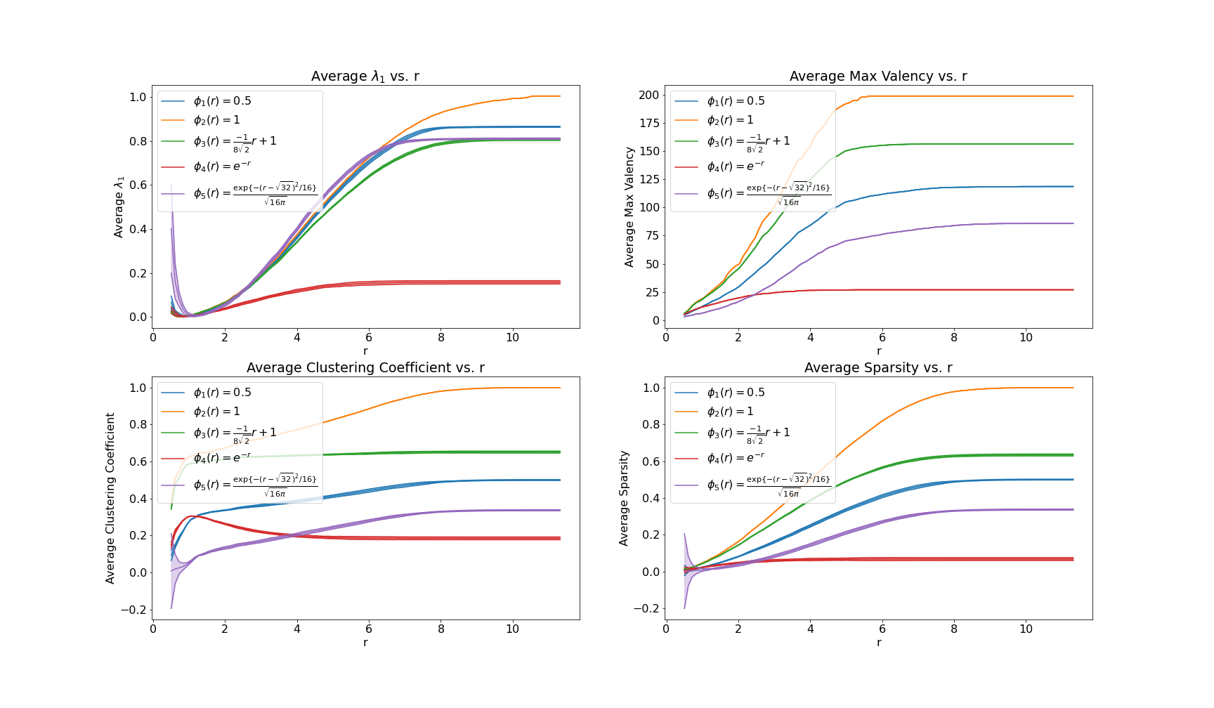
For our first simulation, we will explore some statistical quantities for horospherical random graphs with five different probability parameter functions $p_{i}$ for $i=1,\ldots 5$. In this case, we generate a single random set of 200 points sampled uniformly from an 8 by 8 square. For each probability parameter and each point set, we generate 20 horospherical random graphs by adding a level at each of 100 evenly spaced values of $r$ between 0 and $8\sqrt{2}$. For each level we recorded the values of $\lambda_{1}$, maximum valency, average valency, and sparsity. Our goal is to explore the similarities in the different choices of $p_{i}$ within and across the different point sets as well as the variance in these selections. Figure 1 contains four plots, one for each of these statistics. Each plot contains the average value considered along with a band of one standard deviation for each probability parameter function. These functions consist of two constant functions, $\phi_{1}(r)=0.5$ and $\phi_{2}(r)=1$, an affine function $\phi_{3}(r)=\frac{-r}{8\sqrt{2}}+1$, an exponential $\phi_{4}(r)=e^{-r}$, and $\phi_{5}(r)=\frac{\exp\{-(r-\sqrt{32})^{2}/16\}}{\sqrt{16\pi}}$, a normal density with mean $\sqrt{32}$ and standard deviation $2$.

Figure 1. Four plots of graph properties over 5 different connection functions. For each connection function and each property, the given property was averaged over 20 iterations on a uniformly distributed set, then plotted with a band of one standard deviation.

5.2. A model for mainland France

We construct a model of mainland France by selecting the most populated metropolitan areas such as Paris, Toulouse, Bordeaux, Lyon, Strasbourg, Nantes, Lille, and Côte d’Azur (comprised of Nice, Marseille, and Toulon), using the picture from Wikipedia copied on an $8\times 8$ square. The vertices of our graph sequence were drawn from bivariate normal distributions centered at each of those cities. The number of points drawn from each city is proportional to the population of the city relative to the population of mainland France. Finally, we overlayed a grid of 60 by 60 points (so a mesh of 8/60 ¡0.15) to represent the distribution of the remaining population throughout the country side, and will allow us to force all graphs to be connected. Figure 2 depicts the resulting vertices, 6’000 dots, so that each point is then roughly 10’000 people if we estimate mainland France population by 60 million.

Figure 2. The vertex set $X$, obtained with a simulation of major metropolitan areas of mainland France along with a grid of points representing the rest of the population.

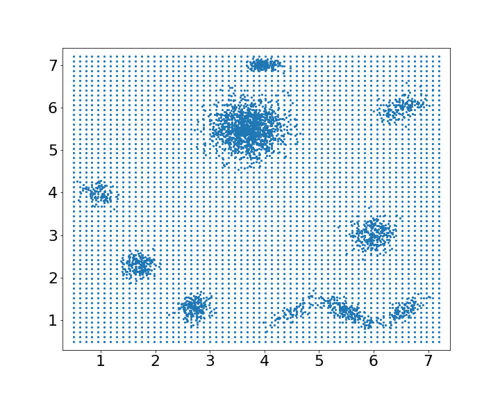
On this set of vertices, denoted by $X$, we compute several simulations with four different connection functions, named $U,C,S$ and $I$, heuristically depicting daily people movements in different situations, and that we now describe. First, we consider the connection function given by

$$U(r)=\begin{cases}1&r\leq 0.15\\ 0.05&0.15<r\leq 0.3\\ 0.03&0.3<r\leq 1\\ 0.02&1<r\leq 3\\ 0.01&3<r\leq 10\\ \end{cases}$$

with the corresponding random graph $\Gamma_{U}=(X,E_{10})$. This corresponds to a daily situation that we estimated very roughly using 2019 official data available on-line before any type of lockdown. Next, we consider the connection function given by

$$S(r)=\begin{cases}1&r\leq 0.15\\ 0.1&0.15<r\leq 0.3\\ 0.05&0.3<r\leq 1\\ 0.01&1<r\leq 3\\ 0.005&3<r\leq 10\\ \end{cases}$$

with corresponding graph $\Gamma_{S}=(X,E_{10})$. This corresponds to some soft travel restrictions, simulating the case where all means of travel are open, but are operating at limited capacity. The connection function

$$C(r)=\begin{cases}1&r\leq 0.15\\ 0.05&0.15<r\leq 0.3\\ 0.003&0.3<r\leq 1\\ 0.002&1<r\leq 3\\ 0.001&3<r\leq 10\\ \end{cases}$$

corresponds to our estimates of long distance travels in France during the 2020 first lockdown, one of the hardest ones, where some 90 percent of airplane activity was cancelled, with the corresponding random graph $\Gamma_{C}=(X,E_{10})$. Finally the connection function

$$I(r)=\begin{cases}1&r\leq 0.3\\ 0&\hbox{otherwise}\end{cases}$$

with corresponding graph $\Gamma_{I}=(X,E_{10})$. This corresponds to a theoretical lockdown, where long distance travel is completely stopped but locally, everything is widely open, without restrictions. In that way, travel between cities is eventually possible, but takes place at a very slow pace.

We seek to compare these graphs through various statistics. Specifically, for each graph we compute the first eigenvalue $\lambda_{1}$, Sparsity, Max Valency, and Average Valency. Because $X$ is fixed and $p_{1}\equiv 1$, the graph $\Gamma_{I}$ is not random, and the probability 1 for $r_{1}\leq 0.15$ on all the graphs is to ensure that those graphs are connected. However, the next layers in the graphs $\Gamma_{U},\Gamma_{S}$ and $\Gamma_{C}$ are random; thus, we choose to compute 20 iterations and average the relevant statistics. The results are summarized in Table 1. We can see that the graphs are nearly equal in Sparsity, except for $\Gamma_{C}$, the hard confinement graph which is much more sparse than the three others and has significantly lower max and average valency while its first eigenvalue $\lambda_{1}$ is roughly a third of the ones in the unconfined graph $\Gamma_{U}$ and the lightly confined model $\Gamma_{S}$. But comparing it to $\Gamma_{I}$, we notice that $\lambda_{1}(\Gamma_{I})$ is $3.5\times 10^{-4}$, so several orders of magnitude smaller than the other graphs. This indicates that random walks on $\Gamma_{I}$ (and unsurprisingly on, $\Gamma_{U}$ and $\Gamma_{S}$) will spread much faster than random walks on $\Gamma_{I}$.

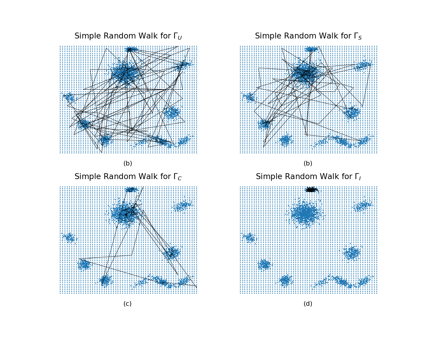
To illustrate this, we consider two different types of random walks. First, we simulate a simple random walk on the four graphs. For each graph, we generate 100 different 100-step random walks with a random starting points. For each walk, we compute the average and maximum pairwise distances. These numbers suggest that traveling long distances is much easier to achieve in the set up for $\Gamma_{C}$ than for that of $\Gamma_{I}$. We summarize these numbers in Table 2. Figure 3 illustrates an example walk resulting from the simulation. We can see that, as expected, the walk for $\Gamma_{U}$ very quickly spreads everywhere, while the walk for $\Gamma_{I}$ remains concentrated near its inception. What is interesting is the fact that for $\Gamma_{S}$ and $\Gamma_{C}$, the walk spreads pretty much everywhere as well.

	$\Gamma_{U}$	$\Gamma_{S}$	$\Gamma_{C}$	$\Gamma_{I}$
$\lambda_{1}$	0.46	0.29	0.09	0.00035
Sparsity	0.019	0.016	0.006	0.015
Max Valency	280	278	178	470
Average Valency	121	96	40	97
Clustering Coefficient	0.06	0.08	0.19	0.62

Table 1. Various statistics for $\Gamma_{U},\Gamma_{S},\Gamma_{C}$ and $\Gamma_{I}$.

	$\Gamma_{U}$	$\Gamma_{S}$	$\Gamma_{C}$	$\Gamma_{I}$
Mean of mean distances	3.07	2.87	2.57	0.27
St. dev. of mean distances	0.23	0.35	0.63	0.20
Mean of max distances	8.2	7.84	7.2	0.91
St. dev. of max distances	0.43	0.53	0.64	0.49

Table 2. Various statistics for 100 walks on $\Gamma_{U},\Gamma_{S},\Gamma_{C}$ and $\Gamma_{I}$

Figure 3. A simple random walk on $\Gamma_{U},\Gamma_{S},\Gamma_{C}$ and $\Gamma_{I}$.

Figure 4. A replicating random walk simulation on $\Gamma_{U},\Gamma_{S},\Gamma_{C}$ and $\Gamma_{I}$.

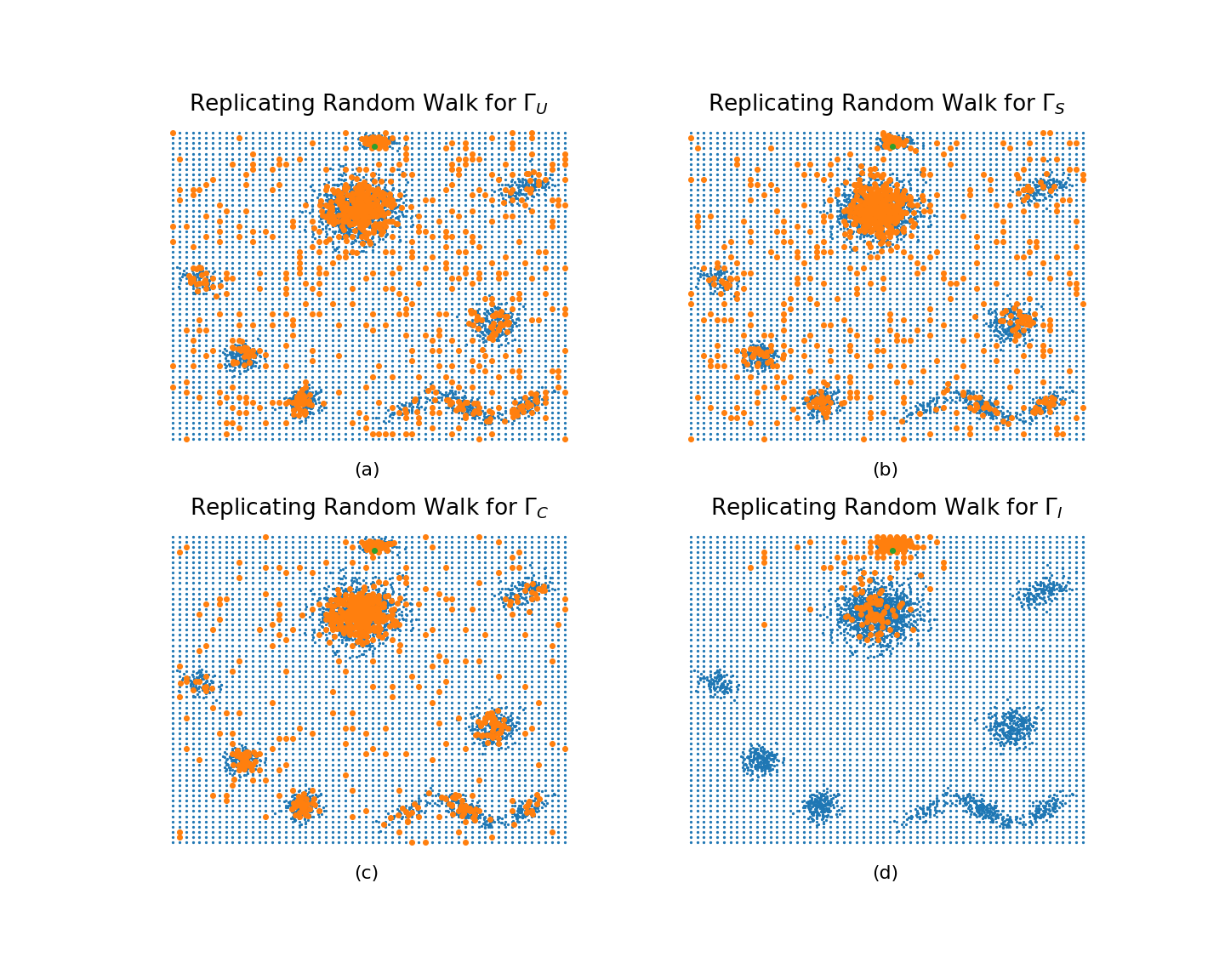
For another illustration, we compute a replicating random walk. The walk for each graph begins with one replicant in the same starting location (near Lille, on the top of the grid). The walk replicates after 10 steps for each replicant visiting a node that has not been replicated before. This walk proceeds for 100 steps. Figure 4 shows the initial positions of each replicant node at the end of the replicating walk. Again, the difference in spread between the different graphs are clear.

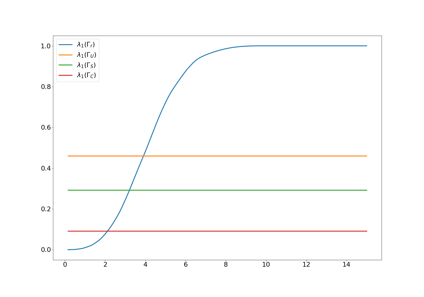
Finally, we explore the effect of the distance parameter, $r$ when $p\equiv 1$, which we will denote as $\Gamma(r)$. Clearly, as $r$ increases, $\lambda_{1}(\Gamma(r))$ will increase as well. Figure 5 shows the behavior of $\lambda_{1}(\Gamma(r))$ in relation to $r$. The orange line in the Figure is $\lambda_{1}(\Gamma_{U})$, the green line is $\lambda_{1}(\Gamma_{S})$ and the red line is $\lambda_{1}(\Gamma_{C})$, the lowest eigenvalue. It is interesting to note that the $\lambda_{1}(\Gamma(r))=\lambda_{1}(\Gamma_{C})$ when $r\approx 2.3$. In our model, this equates to a distance of about 300 km, or 180 miles.

Figure 5. A graph of $\lambda_{1}(\Gamma(r))$. The horizontal line are $\lambda_{1}(\Gamma_{U}),\lambda_{1}(\Gamma_{S})$ and $\lambda_{1}(\Gamma_{C})$.

6. Discussion on the findings and future work

The presence of edges between far away points dramatically increases the speed at which the random walk visits all the vertices of the graph. From the view point of the random walks, completely shutting down medium and long distance travel (which amounts to looking at low level graphs) is more efficient in slowing down the spread of the walk than restricting local interactions. In fact even with high local clustering coefficient, corresponding to a level one graph with large edge probability, the random walk is much slower than in a sparse graph with edges linking far away points.

Our findings show that completely cutting travels over 300 kilometers would give a random walk much slower to spread than in a graph with strict local confinement, amounting to low average valency. Of course, at small scale a high local clustering coefficient would give a high local spread once the walk has reached a location.

Low level graphs, with small first eigenvalue $\lambda_{1}$, also have small conductance and are easy to cut into pieces of similar sizes, meaning that clusters could be disconnected from the rest of the graph. In terms of random walks, this partial confinement mitigates the damages: if the random walk is slow enough, one can divide a graph in $n$ pieces $R_{1},\dots,R_{n}$ easily disconnected by cutting relatively few edges. Compared to their sizes, the $R_{i}$’s have small isoperimetric inequality, meaning that to isolate a piece $R_{i}$ of the rest of the graph to trap the random walk there can be done removing relatively few edges. This can be seen in the graph $\Gamma_{I}$, where the replicating walk starting in Lille doesn’t spread beyond Paris, whereas on $\Gamma_{U},\Gamma_{S}$ and even on $\Gamma_{C}$ it has spread everywhere.

The impact of long distance travel in the spread of diseases is probably well-known by specialists, and the mathematics described in this paper are very classical, but the conclusions seem to be controversial, even if a scientific consensus along those lines seems to emerge [1].

Obviously, comparing our model with actual data, making finer estimates and more accurate models would be interesting and could provide interesting information, but beyond our computing capacity.

References

- [1] Aniruddha Adiga, Srinivasan Venkatramanan, James Schlitt, Akhil Peddireddy, Allan Dickerman, Andrei Bura, Andrew Warren, Brian D Klahn, Chunhong Mao, Dawen Xie, Dustin Machi, Erin Raymond, Fanchao Meng, Golda Barrow, Henning Mortveit, Jiangzhuo Chen, Jim Walke, Joshua Goldstein, Mandy L Wilson, Mark Orr, Przemyslaw Porebski, Pyrros A Telionis, Richard Beckman, Stefan Hoops, Stephen Eubank, Young Yun Baek, Bryan Lewis, Madhav Marathe, and Chris Barrett. Evaluating the impact of international airline suspensions on the early global spread of covid-19. medRxiv, 2020.
- [2] Karl Bringmann, Ralph Keusch, and Johannes Lengler. Geometric inhomogeneous random graphs. Theoretical Computer Science, 760:35–54, 2019.
- [3] Steve Butler, Fan Chung, et al. Spectral graph theory. Handbook of linear algebra, page 47, 2006.
- [4] D. M. Cvetković, M. Doob, and H. Sachs. Spectra of Graphs. 3rd revised and enlarged edition. Heidelberg/Leipzig, Johann Ambrosius Barth Verlag, 1995.
- [5] Richard Durrett. Random graph dynamics, volume 200. Cambridge university press Cambridge, 2007.
- [6] Mikhael Gromov. Hyperbolic groups. In Essays in group theory, pages 75–263. Springer, 1987.
- [7] Luca Gugelmann, Konstantinos Panagiotou, and Ueli Peter. Random hyperbolic graphs: degree sequence and clustering. In 39th International Colloquium on Automata, Languages, and Programming (ICALP), page 573–585, 2012.
- [8] Mounia Hamidouche. Spectral analysis of random geometric graphs. PhD thesis, Université Côte d’Azur, 2020.
- [9] Emmanuel Kowalski. An introduction to expander graphs. Société mathématique de France, 2019.
- [10] David A Levin and Yuval Peres. Markov chains and mixing times, volume 107. American Mathematical Soc., 2017.
- [11] Amy Nyberg. The Laplacian spectra of random geometric graphs. PhD thesis, University of Houston, 2014.
- [12] Mathew D Penrose. Connectivity of soft random geometric graphs. The Annals of Applied Probability, 26(2):986–1028, 2016.
- [13] Remco van der Hofstad, Pim van der Hoorn, and Neeladri Maitra. Local limits of spatial inhomogeneous random graphs. arXiv preprint arXiv:2107.08733, 2021.
- [14] Jie Wu and Duncan J Watts. Small worlds: the dynamics of networks between order and randomness. Acm Sigmod Record, 31(4):74–75, 2002.