2 Problem Formulation
Consider n 𝑛 n ℱ = { 1 , … n } ℱ 1 … 𝑛 \mathcal{F}=\{1,...n\}
η F , i = [ p F , i T , θ F , i ] T , ∀ i ∈ ℱ , formulae-sequence subscript 𝜂 𝐹 𝑖
superscript superscript subscript 𝑝 𝐹 𝑖
𝑇 subscript 𝜃 𝐹 𝑖
𝑇 for-all 𝑖 ℱ \eta_{F,i}=[p_{F,i}^{T},\theta_{F,i}]^{T},\forall i\in\mathcal{F}, (2)
where p F , i = [ x F , i , y F , i ] T subscript 𝑝 𝐹 𝑖
superscript subscript 𝑥 𝐹 𝑖
subscript 𝑦 𝐹 𝑖
𝑇 p_{F,i}=[x_{F,i},y_{F,i}]^{T} θ F , i subscript 𝜃 𝐹 𝑖
\theta_{F,i} (Brockett, 1983 ) for the existence of smooth time-invariant stabilizer. Typical nonholonomic planar vehicles include wheeled mobile robots (Yan and Ma, 2020 ) , underactuated surface vehicles(Ma, 2009 ) and underactuated hovercrafts (Yan et al., 2021 ) .
Besides n 𝑛 n m 𝑚 m n + 1 𝑛 1 n+1 n + m 𝑛 𝑚 n+m
η L , j ( t ) = η c ( t ) + d L , j ∈ ℝ 3 , j ∈ ℛ = { n + 1 , … , n + m } , formulae-sequence subscript 𝜂 𝐿 𝑗
𝑡 subscript 𝜂 𝑐 𝑡 subscript 𝑑 𝐿 𝑗
superscript ℝ 3 𝑗 ℛ 𝑛 1 … 𝑛 𝑚 {\eta_{L,j}}\left(t\right)={\eta_{c}}\left(t\right)+{d_{L,j}}\in\mathbb{R}^{3},j\in\mathcal{R}=\{n+1,...,n+m\}, (3)
where η L , j ( t ) = [ p L , j T ( t ) , θ L , j ( t ) ] T , η c ( t ) = [ p c T ( t ) , θ c ( t ) ] T formulae-sequence subscript 𝜂 𝐿 𝑗
𝑡 superscript superscript subscript 𝑝 𝐿 𝑗
𝑇 𝑡 subscript 𝜃 𝐿 𝑗
𝑡 𝑇 subscript 𝜂 𝑐 𝑡 superscript superscript subscript 𝑝 𝑐 𝑇 𝑡 subscript 𝜃 𝑐 𝑡 𝑇 {\eta_{L,j}}\left(t\right)=[p_{L,j}^{T}(t),\theta_{L,j}(t)]^{T},{\eta_{c}}\left(t\right)={\left[{p_{c}^{T}\left(t\right),{\theta_{c}}\left(t\right)}\right]^{T}} d L , j = [ d L , j p T , d L , j θ ] T ∈ ℝ 3 subscript 𝑑 𝐿 𝑗
superscript superscript subscript 𝑑 𝐿 𝑗 𝑝
𝑇 subscript 𝑑 𝐿 𝑗 𝜃
𝑇 superscript ℝ 3 {d_{L,j}}={\left[{d_{L,jp}^{T},{d_{L,j\theta}}}\right]^{T}}\in\mathbb{R}^{3} d L , j p = [ d L , j x , d j y ] T subscript 𝑑 𝐿 𝑗 𝑝
superscript subscript 𝑑 𝐿 𝑗 𝑥
subscript 𝑑 𝑗 𝑦 𝑇 d_{L,jp}=[d_{L,jx},d_{jy}]^{T} p L , j = [ x L , j , y L , j ] T subscript 𝑝 𝐿 𝑗
superscript subscript 𝑥 𝐿 𝑗
subscript 𝑦 𝐿 𝑗
𝑇 p_{L,j}=[x_{L,j},y_{L,j}]^{T} θ L , j subscript 𝜃 𝐿 𝑗
\theta_{L,j} j 𝑗 j
Assumption 2
The η c ( t ) subscript 𝜂 𝑐 𝑡 \eta_{c}(t)
Assumption 3
The m 𝑚 m d L , j p , ∀ j ∈ ℛ subscript 𝑑 𝐿 𝑗 𝑝
for-all 𝑗
ℛ d_{L,jp},\forall j\in\mathcal{R} m − limit-from 𝑚 m- 0 ∈ [ min { d L , j θ } , max { d L , j θ } ] , ∀ j ∈ ℛ formulae-sequence 0 subscript 𝑑 𝐿 𝑗 𝜃
subscript 𝑑 𝐿 𝑗 𝜃
for-all 𝑗 ℛ 0\in[\min\{d_{L,j\theta}\},\max\{d_{L,j\theta}\}],\forall j\in\mathcal{R}
Define two convex sets formed by leader coordinates (3
𝒞 L p = { [ x , y ] ∈ ℝ 2 | [ x , y ] T = ∑ j = n + 1 n + m b p , j p L , j } , 𝒞 L θ = { θ ∈ ℝ | θ = ∑ j = n + 1 n + m b p , j θ L , j } , formulae-sequence subscript 𝒞 𝐿 𝑝 conditional-set 𝑥 𝑦 superscript ℝ 2 superscript 𝑥 𝑦 𝑇 superscript subscript 𝑗 𝑛 1 𝑛 𝑚 subscript 𝑏 𝑝 𝑗
subscript 𝑝 𝐿 𝑗
subscript 𝒞 𝐿 𝜃 conditional-set 𝜃 ℝ 𝜃 superscript subscript 𝑗 𝑛 1 𝑛 𝑚 subscript 𝑏 𝑝 𝑗
subscript 𝜃 𝐿 𝑗
\begin{split}{\mathcal{C}_{Lp}}&=\left\{{\left.{\left[{x,y}\right]\in{\mathbb{R}^{2}}}\right|\left[{x,y}\right]^{T}=\sum\limits_{j=n+1}^{n+m}{{b_{p,j}}p_{L,j}}}\right\},\mathcal{C}_{L\theta}=\left\{{\left.{\theta\in{\mathbb{R}}}\right|\theta=\sum\limits_{j=n+1}^{n+m}{{b_{p,j}}\theta_{L,j}}}\right\},\end{split} (4)
where b p , j subscript 𝑏 𝑝 𝑗
b_{p,j} b p , j ∈ ℝ [ 0 , 1 ] subscript 𝑏 𝑝 𝑗
subscript ℝ 0 1 b_{p,j}\in\mathbb{R}_{[0,1]} ∑ j = n + 1 n + m b p , j = 1 superscript subscript 𝑗 𝑛 1 𝑛 𝑚 subscript 𝑏 𝑝 𝑗
1 \sum\limits_{j=n+1}^{n+m}{{b_{p,j}}=1}
Define
η F , i r = [ p F , i r T , θ F , i r ] T ∈ ℝ 3 , ∀ i ∈ ℱ . formulae-sequence subscript 𝜂 𝐹 𝑖 𝑟
superscript superscript subscript 𝑝 𝐹 𝑖 𝑟
𝑇 subscript 𝜃 𝐹 𝑖 𝑟
𝑇 superscript ℝ 3 for-all 𝑖 ℱ \eta_{F,ir}=[p_{F,ir}^{T},\theta_{F,ir}]^{T}\in\mathbb{R}^{3},\forall i\in\mathcal{F}. (5)
where p F , i r = [ x F , i r , y F , i r ] T subscript 𝑝 𝐹 𝑖 𝑟
superscript subscript 𝑥 𝐹 𝑖 𝑟
subscript 𝑦 𝐹 𝑖 𝑟
𝑇 p_{F,ir}=[x_{F,ir},y_{F,ir}]^{T} θ F , i r subscript 𝜃 𝐹 𝑖 𝑟
\theta_{F,ir}
Then, the problem is formally stated as: Under Assumptions 1-3, design a virtual reference signal for the holonomic vehicles and derive the conditions within which the nonholonomic vehicles can converge into the convex hull spanned by leaders.
3 Reference Design and Stability Analysis
Let us design
{ η ˙ F , i r = φ F , i r , φ ˙ F , i r = ρ F , i r , ρ ˙ F , i r = − g 1 φ F , i r − g 2 ρ F , i r − g 3 s F , i r − g 4 s F , i r ‖ s F , i r ‖ 2 + γ 1 2 e − 2 γ 2 t , \left\{\begin{split}{{\dot{\eta}}_{F,ir}}&={\varphi_{F,ir}},\\
{{\dot{\varphi}}_{F,ir}}&={\rho_{F,ir}},\\
{{\dot{\rho}}_{F,ir}}&=-{g_{1}}{\varphi_{F,ir}}-{g_{2}}{\rho_{F,ir}}-{g_{3}}{s_{F,ir}}-{g_{4}}\frac{{{s_{F,ir}}}}{{\sqrt{{{\left\|{{s_{F,ir}}}\right\|}^{2}}+{\gamma_{1}}^{2}{e^{-2{\gamma_{2}}t}}}}},\end{split}\right. (6)
where η F , i r ≜ [ p F , i r T , θ F , i r ] T , g 1 > 0 , g 2 > 0 , g 3 > 0 , g 4 > 0 , γ 1 > 0 , γ 2 > 0 formulae-sequence ≜ subscript 𝜂 𝐹 𝑖 𝑟
superscript superscript subscript 𝑝 𝐹 𝑖 𝑟
𝑇 subscript 𝜃 𝐹 𝑖 𝑟
𝑇 formulae-sequence subscript 𝑔 1 0 formulae-sequence subscript 𝑔 2 0 formulae-sequence subscript 𝑔 3 0 formulae-sequence subscript 𝑔 4 0 formulae-sequence subscript 𝛾 1 0 subscript 𝛾 2 0 \eta_{F,ir}\triangleq[p_{F,ir}^{T},\theta_{F,ir}]^{T},g_{1}>0,g_{2}>0,g_{3}>0,g_{4}>0,\gamma_{1}>0,\gamma_{2}>0
s F , i r = ∑ j = 1 n a i j ( ρ F , i r − ρ F , j r ) + g 1 ∑ j = 1 n a i j ( φ F , i r − φ F , j r ) + g 2 ∑ j = 1 n a i j ( η F , i r − η F , j r ) + ∑ j = n + 1 n + m a i j ( ρ F , i r − η ¨ L , j ) + g 1 ∑ j = n + 1 n + m a i j ( φ F , i r − η ˙ L , j ) + g 2 ∑ j = n + 1 n + m a i j ( η F , i r − η ~ L , j ) , subscript 𝑠 𝐹 𝑖 𝑟
superscript subscript 𝑗 1 𝑛 subscript 𝑎 𝑖 𝑗 subscript 𝜌 𝐹 𝑖 𝑟
subscript 𝜌 𝐹 𝑗 𝑟
subscript 𝑔 1 superscript subscript 𝑗 1 𝑛 subscript 𝑎 𝑖 𝑗 subscript 𝜑 𝐹 𝑖 𝑟
subscript 𝜑 𝐹 𝑗 𝑟
subscript 𝑔 2 superscript subscript 𝑗 1 𝑛 subscript 𝑎 𝑖 𝑗 subscript 𝜂 𝐹 𝑖 𝑟
subscript 𝜂 𝐹 𝑗 𝑟
superscript subscript 𝑗 𝑛 1 𝑛 𝑚 subscript 𝑎 𝑖 𝑗 subscript 𝜌 𝐹 𝑖 𝑟
subscript ¨ 𝜂 𝐿 𝑗
subscript 𝑔 1 superscript subscript 𝑗 𝑛 1 𝑛 𝑚 subscript 𝑎 𝑖 𝑗 subscript 𝜑 𝐹 𝑖 𝑟
subscript ˙ 𝜂 𝐿 𝑗
subscript 𝑔 2 superscript subscript 𝑗 𝑛 1 𝑛 𝑚 subscript 𝑎 𝑖 𝑗 subscript 𝜂 𝐹 𝑖 𝑟
subscript ~ 𝜂 𝐿 𝑗
\begin{split}{s_{F,ir}}&=\sum\limits_{j=1}^{n}{{a_{ij}}\left({{\rho_{F,ir}}-{\rho_{F,jr}}}\right)}+{g_{1}}\sum\limits_{j=1}^{n}{{a_{ij}}\left({{\varphi_{F,ir}}-{\varphi_{F,jr}}}\right)}\\
&~{}+{g_{2}}\sum\limits_{j=1}^{n}{{a_{ij}}\left({{\eta_{F,ir}}-{\eta_{F,jr}}}\right)}+\sum\limits_{j=n+1}^{n+m}{{a_{ij}}\left({{\rho_{F,ir}}-{{\ddot{\eta}}_{L,j}}}\right)}\\
&~{}+{g_{1}}\sum\limits_{j=n+1}^{n+m}{{a_{ij}}\left({{\varphi_{F,ir}}-{{\dot{\eta}}_{L,j}}}\right)}+{g_{2}}\sum\limits_{j=n+1}^{n+m}{{a_{ij}}\left({\eta_{F,ir}}-\tilde{\eta}_{L,j}\right)},\end{split} (7)
where η ~ L , j = η c ( t ) + μ d L , j subscript ~ 𝜂 𝐿 𝑗
subscript 𝜂 𝑐 𝑡 𝜇 subscript 𝑑 𝐿 𝑗
\tilde{{\eta}}_{L,j}=\eta_{c}(t)+\mu d_{L,j} 0 < μ < 1 0 𝜇 1 0<\mu<1
Theorem 1
Given Assumptions 2 1 g 1 > 0 , g 2 > 0 , g 3 > 0 , g 4 ≥ n η ¯ c , η ¯ c = sup t ≥ 0 ‖ η ˙˙˙ c + g 1 η ¨ c + g 2 η ˙ c ‖ , γ 1 > 0 formulae-sequence subscript 𝑔 1 0 formulae-sequence subscript 𝑔 2 0 formulae-sequence subscript 𝑔 3 0 formulae-sequence subscript 𝑔 4 𝑛 subscript ¯ 𝜂 𝑐 formulae-sequence subscript ¯ 𝜂 𝑐 subscript supremum 𝑡 0 norm subscript ˙˙˙ 𝜂 𝑐 subscript 𝑔 1 subscript ¨ 𝜂 𝑐 subscript 𝑔 2 subscript ˙ 𝜂 𝑐 subscript 𝛾 1 0 g_{1}>0,g_{2}>0,g_{3}>0,g_{4}\geq n\bar{\eta}_{c},\bar{\eta}_{c}=\mathop{\sup}\limits_{t\geq 0}\left\|{\dddot{\eta}_{c}+{g_{1}}{\ddot{\eta}}_{c}+{g_{2}}{\dot{\eta}}_{c}}\right\|,\gamma_{1}>0 γ 2 > 0 subscript 𝛾 2 0 \gamma_{2}>0 η F , i r = [ p F , i r T , θ F , i r ] T , ∀ i ∈ ℱ formulae-sequence subscript 𝜂 𝐹 𝑖 𝑟
superscript superscript subscript 𝑝 𝐹 𝑖 𝑟
𝑇 subscript 𝜃 𝐹 𝑖 𝑟
𝑇 for-all 𝑖 ℱ \eta_{F,ir}=[p_{F,ir}^{T},\theta_{F,ir}]^{T},\forall i\in\mathcal{F} 6
lim t → + ∞ η F , r = − ( ℒ 1 − 1 ℒ 2 ⊗ I 3 ) η ~ L , subscript → 𝑡 subscript 𝜂 𝐹 𝑟
tensor-product superscript subscript ℒ 1 1 subscript ℒ 2 subscript 𝐼 3 subscript ~ 𝜂 𝐿 \mathop{\lim}\limits_{t\to+\infty}{\eta_{F,r}}=-\left({\mathcal{L}_{1}^{-1}{\mathcal{L}_{2}}\otimes{I_{3}}}\right)\tilde{\eta}_{L}, (8)
where
η F , r ≜ [ η F , 1 r T , … , η F , n r T ] T ∈ ℝ 3 n , η ~ L ≜ [ η ~ n + 1 T , … , η ~ n + m T ] T ∈ ℝ 3 m . formulae-sequence ≜ subscript 𝜂 𝐹 𝑟
superscript superscript subscript 𝜂 𝐹 1 𝑟
𝑇 … superscript subscript 𝜂 𝐹 𝑛 𝑟
𝑇
𝑇 superscript ℝ 3 𝑛 ≜ subscript ~ 𝜂 𝐿 superscript superscript subscript ~ 𝜂 𝑛 1 𝑇 … superscript subscript ~ 𝜂 𝑛 𝑚 𝑇
𝑇 superscript ℝ 3 𝑚 \begin{split}\eta_{F,r}&\triangleq[\eta_{F,1r}^{T},...,\eta_{F,nr}^{T}]^{T}\in\mathbb{R}^{3n},\tilde{\eta}_{L}\triangleq[\tilde{\eta}_{n+1}^{T},...,\tilde{\eta}_{n+m}^{T}]^{T}\in\mathbb{R}^{3m}.\end{split}
Proof.
Define three stacked vectors belonging to ℝ 3 n superscript ℝ 3 𝑛 \mathbb{R}^{3n}
φ F , r = [ φ F , 1 r T , … , φ F , n r T ] T , ρ F , r = [ ρ F , 1 r T , … , ρ F , n r T ] T , s F , r = [ s F , 1 r T , … , s F , n r T ] T . formulae-sequence subscript 𝜑 𝐹 𝑟
superscript superscript subscript 𝜑 𝐹 1 𝑟
𝑇 … superscript subscript 𝜑 𝐹 𝑛 𝑟
𝑇
𝑇 formulae-sequence subscript 𝜌 𝐹 𝑟
superscript superscript subscript 𝜌 𝐹 1 𝑟
𝑇 … superscript subscript 𝜌 𝐹 𝑛 𝑟
𝑇
𝑇 subscript 𝑠 𝐹 𝑟
superscript superscript subscript 𝑠 𝐹 1 𝑟
𝑇 … superscript subscript 𝑠 𝐹 𝑛 𝑟
𝑇
𝑇 \begin{split}\varphi_{F,r}&=[\varphi_{F,1r}^{T},...,\varphi_{F,nr}^{T}]^{T},\rho_{F,r}=[\rho_{F,1r}^{T},...,\rho_{F,nr}^{T}]^{T},s_{F,r}=[s_{F,1r}^{T},...,s_{F,nr}^{T}]^{T}.\end{split} (9)
By (1 7
{ η ˙ F , r = φ F , r , φ ˙ F , r = ρ F , r , ρ ˙ F , r = − g 1 φ F , r − g 2 ρ F , r − g 3 s F , r − g 4 P F s F , r , \left\{\begin{split}{{\dot{\eta}}_{F,r}}&={\varphi_{F,r}},\\
{{\dot{\varphi}}_{F,r}}&={\rho_{F,r}},\\
{{\dot{\rho}}_{F,r}}&=-{g_{1}}{\varphi_{F,r}}-{g_{2}}{\rho_{F,r}}-{g_{3}}{s_{F,r}}-{g_{4}}P_{F}{s_{F,r}},\end{split}\right. (10)
where P F = diag { [ 𝟏 3 T ‖ s F , 1 d ‖ 2 + γ 1 2 e − 2 γ 2 t , … , 𝟏 3 T ‖ s F , n d ‖ 2 + γ 1 2 e − 2 γ 2 t ] } ∈ ℝ 3 n × 3 n subscript 𝑃 𝐹 diag superscript subscript 1 3 𝑇 superscript norm subscript 𝑠 𝐹 1 𝑑
2 superscript subscript 𝛾 1 2 superscript 𝑒 2 subscript 𝛾 2 𝑡 … superscript subscript 1 3 𝑇 superscript norm subscript 𝑠 𝐹 𝑛 𝑑
2 superscript subscript 𝛾 1 2 superscript 𝑒 2 subscript 𝛾 2 𝑡
superscript ℝ 3 𝑛 3 𝑛 P_{F}=\mathrm{diag}\{[\frac{\mathbf{1}_{3}^{T}}{\sqrt{\|s_{F,1d}\|^{2}+\gamma_{1}^{2}e^{-2\gamma_{2}t}}},...,\frac{\mathbf{1}_{3}^{T}}{\sqrt{\|s_{F,nd}\|^{2}+\gamma_{1}^{2}e^{-2\gamma_{2}t}}}]\}\in\mathbb{R}^{3n\times 3n} s F , r subscript 𝑠 𝐹 𝑟
{s}_{F,r}
s F , r = ( ℒ 1 ⊗ I 3 ) ( ρ F , r + g 1 φ F , r + g 2 η F , r ) + ( ℒ 2 ⊗ I 3 ) [ η ~ ¨ L + g 1 η ~ ˙ L + g 2 η ~ L ] , subscript 𝑠 𝐹 𝑟
tensor-product subscript ℒ 1 subscript 𝐼 3 subscript 𝜌 𝐹 𝑟
subscript 𝑔 1 subscript 𝜑 𝐹 𝑟
subscript 𝑔 2 subscript 𝜂 𝐹 𝑟
tensor-product subscript ℒ 2 subscript 𝐼 3 delimited-[] subscript ¨ ~ 𝜂 𝐿 subscript 𝑔 1 subscript ˙ ~ 𝜂 𝐿 subscript 𝑔 2 subscript ~ 𝜂 𝐿 \begin{split}{s_{F,r}}&=\left({{\mathcal{L}_{1}}\otimes{I_{3}}}\right)\left({{\rho_{F,r}}+{g_{1}}{\varphi_{F,r}}+{g_{2}}{\eta_{F,r}}}\right)+\left({{\mathcal{L}_{2}}\otimes{I_{3}}}\right)\left[{{{\ddot{\tilde{\eta}}}_{L}}+{g_{1}}{{\dot{\tilde{\eta}}}_{L}}+{g_{2}}\tilde{\eta}_{L}}\right],\end{split} (11)
where the facts η ~ ¨ L = η ¨ L subscript ¨ ~ 𝜂 𝐿 subscript ¨ 𝜂 𝐿 \ddot{\tilde{\eta}}_{L}=\ddot{\eta}_{L} η ~ ˙ L = η ˙ L subscript ˙ ~ 𝜂 𝐿 subscript ˙ 𝜂 𝐿 \dot{\tilde{\eta}}_{L}=\dot{\eta}_{L}
ξ F = η F , r + ( ℒ 1 − 1 ℒ 2 ⊗ I 3 ) η ~ L , subscript 𝜉 𝐹 subscript 𝜂 𝐹 𝑟
tensor-product superscript subscript ℒ 1 1 subscript ℒ 2 subscript 𝐼 3 subscript ~ 𝜂 𝐿 \xi_{F}=\eta_{F,r}+(\mathcal{L}_{1}^{-1}\mathcal{L}_{2}\otimes I_{3})\tilde{\eta}_{L}, (12)
and
𝐒 F = ξ ¨ F + g 1 ξ ˙ F + g 2 ξ F = ρ F , r + ( ℒ 1 − 1 ℒ 2 ⊗ I 3 ) η ~ ¨ L + g 1 [ φ F , r + ( ℒ 1 − 1 ℒ 2 ⊗ I 3 ) η ~ ˙ L ] + g 2 [ η F , r + ( ℒ 1 − 1 ℒ 2 ⊗ I 3 ) η ~ L ] . subscript 𝐒 𝐹 subscript ¨ 𝜉 𝐹 subscript 𝑔 1 subscript ˙ 𝜉 𝐹 subscript 𝑔 2 subscript 𝜉 𝐹 subscript 𝜌 𝐹 𝑟
tensor-product superscript subscript ℒ 1 1 subscript ℒ 2 subscript 𝐼 3 subscript ¨ ~ 𝜂 𝐿 subscript 𝑔 1 delimited-[] subscript 𝜑 𝐹 𝑟
tensor-product superscript subscript ℒ 1 1 subscript ℒ 2 subscript 𝐼 3 subscript ˙ ~ 𝜂 𝐿 subscript 𝑔 2 delimited-[] subscript 𝜂 𝐹 𝑟
tensor-product superscript subscript ℒ 1 1 subscript ℒ 2 subscript 𝐼 3 subscript ~ 𝜂 𝐿 \begin{split}\mathbf{S}_{F}&={{\ddot{\xi}}_{F}}+{g_{1}}{{\dot{\xi}}_{F}}+{g_{2}}{\xi_{F}}\\
&={\rho_{F,r}}+\left({\mathcal{L}_{1}^{-1}{\mathcal{L}_{2}}\otimes{I_{3}}}\right){{\ddot{\tilde{\eta}}}_{L}}+{g_{1}}\left[{{\varphi_{F,r}}+\left({\mathcal{L}_{1}^{-1}{\mathcal{L}_{2}}\otimes{I_{3}}}\right){{\dot{\tilde{\eta}}}_{L}}}\right]+{g_{2}}\left[{{\eta_{F,r}}+\left({\mathcal{L}_{1}^{-1}{\mathcal{L}_{2}}\otimes{I_{3}}}\right)\tilde{\eta}_{L}}\right].\end{split} (13)
By (11 12
s F , r = ( ℒ 1 ⊗ I 3 ) 𝐒 F . subscript 𝑠 𝐹 𝑟
tensor-product subscript ℒ 1 subscript 𝐼 3 subscript 𝐒 𝐹 s_{F,r}=(\mathcal{L}_{1}\otimes I_{3})\mathbf{S}_{F}. (14)
It is obvious that the convergence to zero of 𝐒 F subscript 𝐒 𝐹 \mathbf{S}_{F} ξ F subscript 𝜉 𝐹 \xi_{F} lim t → ∞ η F , r = − ( ℒ 1 − 1 ℒ 2 ⊗ I 3 ) η ~ L subscript → 𝑡 subscript 𝜂 𝐹 𝑟
tensor-product superscript subscript ℒ 1 1 subscript ℒ 2 subscript 𝐼 3 subscript ~ 𝜂 𝐿 \mathop{\lim}\limits_{t\to\infty}\eta_{F,r}=-(\mathcal{L}_{1}^{-1}\mathcal{L}_{2}\otimes I_{3})\tilde{\eta}_{L} 𝐒 F subscript 𝐒 𝐹 \mathbf{S}_{F} t 𝑡 t
𝐒 ˙ F = η ˙˙˙ F , r + ( ℒ 1 − 1 ℒ 2 ⊗ I 3 ) η ~ ˙˙˙ L + g 1 [ η ¨ F , r + ( ℒ 1 − 1 ℒ 2 ⊗ I 3 ) η ~ ¨ L ] + g 2 [ η ˙ F , r + ( ℒ 1 − 1 ℒ 2 ⊗ I 3 ) η ~ ˙ L ] = − g 1 φ F , r − g 2 ρ F , r − g 3 s F , r − g 4 P F s F , r + ( ℒ 1 − 1 ℒ 2 ⊗ I 3 ) η ~ ˙˙˙ L + g 1 [ φ F , r + ( ℒ 1 − 1 ℒ 2 ⊗ I 3 ) η ~ ¨ L ] + g 2 [ ρ F , r + ( ℒ 1 − 1 ℒ 2 ⊗ I 3 ) η ~ ˙ L ] = − g 3 s F , r − g 4 P F s F , r + ( ℒ 1 − 1 ℒ 2 ⊗ I 3 ) ( η ~ ˙˙˙ L + g 1 η ~ ¨ L + g 2 η ~ ˙ L ) = − g 3 ( ℒ 1 ⊗ I 3 ) S F − g 4 P F ( ℒ 1 ⊗ I 3 ) S F + ( ℒ 1 − 1 ℒ 2 ⊗ I 3 ) ( η ~ ˙˙˙ L + g 1 η ~ ¨ L + g 2 η ~ ˙ L ) . subscript ˙ 𝐒 𝐹 subscript ˙˙˙ 𝜂 𝐹 𝑟
tensor-product superscript subscript ℒ 1 1 subscript ℒ 2 subscript 𝐼 3 subscript ˙˙˙ ~ 𝜂 𝐿 subscript 𝑔 1 delimited-[] subscript ¨ 𝜂 𝐹 𝑟
tensor-product superscript subscript ℒ 1 1 subscript ℒ 2 subscript 𝐼 3 subscript ¨ ~ 𝜂 𝐿 subscript 𝑔 2 delimited-[] subscript ˙ 𝜂 𝐹 𝑟
tensor-product superscript subscript ℒ 1 1 subscript ℒ 2 subscript 𝐼 3 subscript ˙ ~ 𝜂 𝐿 subscript 𝑔 1 subscript 𝜑 𝐹 𝑟
subscript 𝑔 2 subscript 𝜌 𝐹 𝑟
subscript 𝑔 3 subscript 𝑠 𝐹 𝑟
subscript 𝑔 4 subscript 𝑃 𝐹 subscript 𝑠 𝐹 𝑟
tensor-product superscript subscript ℒ 1 1 subscript ℒ 2 subscript 𝐼 3 subscript ˙˙˙ ~ 𝜂 𝐿 subscript 𝑔 1 delimited-[] subscript 𝜑 𝐹 𝑟
tensor-product superscript subscript ℒ 1 1 subscript ℒ 2 subscript 𝐼 3 subscript ¨ ~ 𝜂 𝐿 subscript 𝑔 2 delimited-[] subscript 𝜌 𝐹 𝑟
tensor-product superscript subscript ℒ 1 1 subscript ℒ 2 subscript 𝐼 3 subscript ˙ ~ 𝜂 𝐿 subscript 𝑔 3 subscript 𝑠 𝐹 𝑟
subscript 𝑔 4 subscript 𝑃 𝐹 subscript 𝑠 𝐹 𝑟
tensor-product superscript subscript ℒ 1 1 subscript ℒ 2 subscript 𝐼 3 subscript ˙˙˙ ~ 𝜂 𝐿 subscript 𝑔 1 subscript ¨ ~ 𝜂 𝐿 subscript 𝑔 2 subscript ˙ ~ 𝜂 𝐿 subscript 𝑔 3 tensor-product subscript ℒ 1 subscript 𝐼 3 subscript 𝑆 𝐹 subscript 𝑔 4 subscript 𝑃 𝐹 tensor-product subscript ℒ 1 subscript 𝐼 3 subscript 𝑆 𝐹 tensor-product superscript subscript ℒ 1 1 subscript ℒ 2 subscript 𝐼 3 subscript ˙˙˙ ~ 𝜂 𝐿 subscript 𝑔 1 subscript ¨ ~ 𝜂 𝐿 subscript 𝑔 2 subscript ˙ ~ 𝜂 𝐿 \begin{split}{{\dot{\mathbf{S}}}_{F}}&={{\dddot{\eta}}_{F,r}}+\left({\mathcal{L}_{1}^{-1}{\mathcal{L}_{2}}\otimes{I_{3}}}\right){{\dddot{\tilde{\eta}}}_{L}}+{g_{1}}\left[{{{\ddot{\eta}}_{F,r}}+\left({\mathcal{L}_{1}^{-1}{\mathcal{L}_{2}}\otimes{I_{3}}}\right){{\ddot{\tilde{\eta}}}_{L}}}\right]+{g_{2}}\left[{{{\dot{\eta}}_{F,r}}+\left({\mathcal{L}_{1}^{-1}{\mathcal{L}_{2}}\otimes{I_{3}}}\right){{\dot{\tilde{\eta}}}_{L}}}\right]\\
&=-{g_{1}}{\varphi_{F,r}}-{g_{2}}{\rho_{F,r}}-{g_{3}}{s_{F,r}}-{g_{4}}{P_{F}}{s_{F,r}}+\left({\mathcal{L}_{1}^{-1}{\mathcal{L}_{2}}\otimes{I_{3}}}\right){{\dddot{{\tilde{\eta}}}}_{L}}\\
&~{}+{g_{1}}\left[{{\varphi_{F,r}}+\left({\mathcal{L}_{1}^{-1}{\mathcal{L}_{2}}\otimes{I_{3}}}\right){{\ddot{\tilde{\eta}}}_{L}}}\right]+{g_{2}}\left[{{\rho_{F,r}}+\left({\mathcal{L}_{1}^{-1}{\mathcal{L}_{2}}\otimes{I_{3}}}\right){{\dot{\tilde{\eta}}}_{L}}}\right]\\
&=-{g_{3}}{s_{F,r}}-{g_{4}}{P_{F}}{s_{F,r}}+\left({\mathcal{L}_{1}^{-1}{\mathcal{L}_{2}}\otimes{I_{3}}}\right)\left({{{\dddot{\tilde{\eta}}}_{L}}+{g_{1}}{{\ddot{\tilde{\eta}}}_{L}}+{g_{2}}{{\dot{\tilde{\eta}}}_{L}}}\right)\\
&=-{g_{3}}(\mathcal{L}_{1}\otimes I_{3}){S_{F}}-{g_{4}}{P_{F}}(\mathcal{L}_{1}\otimes I_{3}){S_{F}}+\left({\mathcal{L}_{1}^{-1}{\mathcal{L}_{2}}\otimes{I_{3}}}\right)\left({{{\dddot{{\tilde{\eta}}}}_{L}}+{g_{1}}{{\ddot{\tilde{\eta}}}_{L}}+{g_{2}}{{\dot{\tilde{\eta}}}_{L}}}\right).\end{split} (15)
Using the property that ℒ 1 subscript ℒ 1 \mathcal{L}_{1}
V 1 = 0.5 𝐒 F T ( ℒ 1 ⊗ I 3 ) 𝐒 F , subscript 𝑉 1 0.5 superscript subscript 𝐒 𝐹 𝑇 tensor-product subscript ℒ 1 subscript 𝐼 3 subscript 𝐒 𝐹 V_{1}=0.5\mathbf{S}_{F}^{T}(\mathcal{L}_{1}\otimes I_{3})\mathbf{S}_{F}, (16)
which satisfies 0.5 λ min ( ℒ 1 ) ‖ 𝐒 F ‖ 2 ≤ V 1 ≤ 0.5 λ max ( ℒ 1 ) ‖ 𝐒 F ‖ 2 0.5 subscript 𝜆 subscript ℒ 1 superscript norm subscript 𝐒 𝐹 2 subscript 𝑉 1 0.5 subscript 𝜆 subscript ℒ 1 superscript norm subscript 𝐒 𝐹 2 0.5\lambda_{\min}(\mathcal{L}_{1})\|\mathbf{S}_{F}\|^{2}\leq V_{1}\leq 0.5\lambda_{\max}(\mathcal{L}_{1})\|\mathbf{S}_{F}\|^{2} ‖ 𝐒 F ‖ 2 ≥ 2 V 1 λ max ( ℒ 1 ) superscript norm subscript 𝐒 𝐹 2 2 subscript 𝑉 1 subscript 𝜆 subscript ℒ 1 \|\mathbf{S}_{F}\|^{2}\geq 2\frac{V_{1}}{\lambda_{\max}(\mathcal{L}_{1})} 16 15
V ˙ 1 = − g 3 𝐒 F T ( ℒ 1 ⊗ I 3 ) 2 𝐒 F − g 4 P F 𝐒 F T ( ℒ 1 ⊗ I 3 ) 2 𝐒 F + 𝐒 F T ( ℒ 1 ⊗ I 3 ) ( ℒ 1 − 1 ℒ 2 ⊗ I 3 ) ( η ~ ˙˙˙ L + g 1 η ~ ¨ L + g 2 η ~ ˙ L ) = − g 3 𝐒 F T ( ℒ 1 ⊗ I 3 ) 2 𝐒 F − g 4 P 4 s F , r T s F , r + s F , r T ( ℒ 1 − 1 ℒ 2 ⊗ I 3 ) ( η ~ ˙˙˙ L + g 1 η ~ ¨ L + g 2 η ~ ˙ L ) , subscript ˙ 𝑉 1 subscript 𝑔 3 superscript subscript 𝐒 𝐹 𝑇 superscript tensor-product subscript ℒ 1 subscript 𝐼 3 2 subscript 𝐒 𝐹 subscript 𝑔 4 subscript 𝑃 𝐹 superscript subscript 𝐒 𝐹 𝑇 superscript tensor-product subscript ℒ 1 subscript 𝐼 3 2 subscript 𝐒 𝐹 superscript subscript 𝐒 𝐹 𝑇 tensor-product subscript ℒ 1 subscript 𝐼 3 tensor-product superscript subscript ℒ 1 1 subscript ℒ 2 subscript 𝐼 3 subscript ˙˙˙ ~ 𝜂 𝐿 subscript 𝑔 1 subscript ¨ ~ 𝜂 𝐿 subscript 𝑔 2 subscript ˙ ~ 𝜂 𝐿 subscript 𝑔 3 superscript subscript 𝐒 𝐹 𝑇 superscript tensor-product subscript ℒ 1 subscript 𝐼 3 2 subscript 𝐒 𝐹 subscript 𝑔 4 subscript 𝑃 4 superscript subscript 𝑠 𝐹 𝑟
𝑇 subscript 𝑠 𝐹 𝑟
superscript subscript 𝑠 𝐹 𝑟
𝑇 tensor-product superscript subscript ℒ 1 1 subscript ℒ 2 subscript 𝐼 3 subscript ˙˙˙ ~ 𝜂 𝐿 subscript 𝑔 1 subscript ¨ ~ 𝜂 𝐿 subscript 𝑔 2 subscript ˙ ~ 𝜂 𝐿 \begin{split}{\dot{V}}_{1}&=-{g_{3}}\mathbf{S}_{F}^{T}{\left({{\mathcal{L}_{1}}\otimes{I_{3}}}\right)^{2}}{\mathbf{S}_{F}}-{g_{4}}{P_{F}}\mathbf{S}_{F}^{T}{\left({{\mathcal{L}_{1}}\otimes{I_{3}}}\right)^{2}}{\mathbf{S}_{F}}+\mathbf{S}_{F}^{T}\left({{\mathcal{L}_{1}}\otimes{I_{3}}}\right)\left({\mathcal{L}_{1}^{-1}{\mathcal{L}_{2}}\otimes{I_{3}}}\right)\left({{{\dddot{\tilde{\eta}}}_{L}}+{g_{1}}{{\ddot{\tilde{\eta}}}_{L}}+{g_{2}}{\dot{{\tilde{\eta}}}_{L}}}\right)\\
&=-{g_{3}}\mathbf{S}_{F}^{T}{\left({{\mathcal{L}_{1}}\otimes{I_{3}}}\right)^{2}}{\mathbf{S}_{F}}-{g_{4}}{P_{4}}s_{F,r}^{T}{s_{F,r}}+{s_{F,r}^{T}}\left({\mathcal{L}_{1}^{-1}{\mathcal{L}_{2}}\otimes{I_{3}}}\right)\left({{{\dddot{\tilde{\eta}}}_{L}}+{g_{1}}{{\ddot{\tilde{\eta}}}_{L}}+{g_{2}}{\dot{{\tilde{\eta}}}_{L}}}\right),\end{split} (17)
where the equation s F , r T = 𝐒 F T ( ℒ 1 ⊗ I 3 ) superscript subscript 𝑠 𝐹 𝑟
𝑇 superscript subscript 𝐒 𝐹 𝑇 tensor-product subscript ℒ 1 subscript 𝐼 3 s_{F,r}^{T}=\mathbf{S}_{F}^{T}(\mathcal{L}_{1}\otimes I_{3}) − ℒ 1 − 1 ℒ 2 1 m = 1 n superscript subscript ℒ 1 1 subscript ℒ 2 subscript 1 𝑚 subscript 1 𝑛 -\mathcal{L}_{1}^{-1}\mathcal{L}_{2}1_{m}=1_{n}
s F , r T ( ℒ 1 − 1 ℒ 2 ⊗ I 3 ) ( η ~ ˙˙˙ L + g 1 η ~ ¨ L + g 2 η ~ ˙ L ) = s F , r T ( ℒ 1 − 1 ℒ 2 ⊗ I 3 ) [ 1 m ⊗ ( η ˙˙˙ c + g 1 η ¨ c + g 2 η ˙ c ) ] = s F , r T [ ℒ 1 − 1 ℒ 2 1 m ⊗ ( η ˙˙˙ c + g 1 η ¨ c + g 2 η ˙ c ) ] = − s F , r T [ 1 n ⊗ ( η ˙˙˙ c + g 1 η ¨ c + g 2 η ˙ c ) ] ≤ n ∑ i = 1 n ‖ s F , i r T ‖ η ¯ c , superscript subscript 𝑠 𝐹 𝑟
𝑇 tensor-product superscript subscript ℒ 1 1 subscript ℒ 2 subscript 𝐼 3 subscript ˙˙˙ ~ 𝜂 𝐿 subscript 𝑔 1 subscript ¨ ~ 𝜂 𝐿 subscript 𝑔 2 subscript ˙ ~ 𝜂 𝐿 superscript subscript 𝑠 𝐹 𝑟
𝑇 tensor-product superscript subscript ℒ 1 1 subscript ℒ 2 subscript 𝐼 3 delimited-[] tensor-product subscript 1 𝑚 subscript ˙˙˙ 𝜂 𝑐 subscript 𝑔 1 subscript ¨ 𝜂 𝑐 subscript 𝑔 2 subscript ˙ 𝜂 𝑐 superscript subscript 𝑠 𝐹 𝑟
𝑇 delimited-[] tensor-product superscript subscript ℒ 1 1 subscript ℒ 2 subscript 1 𝑚 subscript ˙˙˙ 𝜂 𝑐 subscript 𝑔 1 subscript ¨ 𝜂 𝑐 subscript 𝑔 2 subscript ˙ 𝜂 𝑐 superscript subscript 𝑠 𝐹 𝑟
𝑇 delimited-[] tensor-product subscript 1 𝑛 subscript ˙˙˙ 𝜂 𝑐 subscript 𝑔 1 subscript ¨ 𝜂 𝑐 subscript 𝑔 2 subscript ˙ 𝜂 𝑐 𝑛 superscript subscript 𝑖 1 𝑛 delimited-∥∥ superscript subscript 𝑠 𝐹 𝑖 𝑟
𝑇 subscript ¯ 𝜂 𝑐 \begin{split}s_{F,r}^{T}\left({\mathcal{L}_{1}^{-1}{\mathcal{L}_{2}}\otimes{I_{3}}}\right)\left({{{\dddot{\tilde{\eta}}}_{L}}+{g_{1}}{{\ddot{\tilde{\eta}}}_{L}}+{g_{2}}{{\dot{\tilde{\eta}}}_{L}}}\right)&~{}=s_{F,r}^{T}\left({\mathcal{L}_{1}^{-1}{\mathcal{L}_{2}}\otimes{I_{3}}}\right)\left[1_{m}\otimes(\dddot{\eta}_{c}+g_{1}\ddot{\eta}_{c}+g_{2}\dot{\eta}_{c})\right]\\
&~{}=s_{F,r}^{T}\left[{\mathcal{L}_{1}^{-1}{\mathcal{L}_{2}}1_{m}\otimes(\dddot{\eta}_{c}+g_{1}\ddot{\eta}_{c}+g_{2}\dot{\eta}_{c})}\right]\\
&~{}=-s_{F,r}^{T}\left[{1_{n}\otimes(\dddot{\eta}_{c}+g_{1}\ddot{\eta}_{c}+g_{2}\dot{\eta}_{c})}\right]\\
&~{}\leq n\sum\limits_{i=1}^{n}{\left\|{s_{F,ir}^{T}}\right\|}{{\bar{\eta}}_{c}},\end{split} (18)
where the fact η ~ L , j ( q ) = η c ( q ) ( t ) , ∀ j ∈ ℛ , q ∈ ℤ ≥ 1 formulae-sequence superscript subscript ~ 𝜂 𝐿 𝑗
𝑞 superscript subscript 𝜂 𝑐 𝑞 𝑡 formulae-sequence for-all 𝑗 ℛ 𝑞 subscript ℤ absent 1 \tilde{\eta}_{L,j}^{(q)}=\eta_{c}^{(q)}(t),\forall j\in\mathcal{R},q\in\mathbb{Z}_{\geq 1} 17 18
V ˙ 1 ≤ − g 3 𝐒 F T ( ℒ 1 ⊗ I 3 ) 2 𝐒 F − ∑ i = 1 n g 4 s F , i r T s F , i r ‖ s F , i r ‖ 2 + γ 1 2 e − 2 γ 2 t + ∑ i = 1 n ‖ s F , i r T ‖ n η ¯ c = − g 3 𝐒 F T ( ℒ 1 ⊗ I 3 ) 2 𝐒 F − ∑ i = 1 n ( g 4 ‖ s F , i r ‖ 2 ‖ s F , i r ‖ 2 + γ 1 2 e − 2 γ 2 t − ‖ s F , i r T ‖ n η ¯ c ) . subscript ˙ 𝑉 1 subscript 𝑔 3 superscript subscript 𝐒 𝐹 𝑇 superscript tensor-product subscript ℒ 1 subscript 𝐼 3 2 subscript 𝐒 𝐹 superscript subscript 𝑖 1 𝑛 subscript 𝑔 4 superscript subscript 𝑠 𝐹 𝑖 𝑟
𝑇 subscript 𝑠 𝐹 𝑖 𝑟
superscript norm subscript 𝑠 𝐹 𝑖 𝑟
2 superscript subscript 𝛾 1 2 superscript 𝑒 2 subscript 𝛾 2 𝑡 superscript subscript 𝑖 1 𝑛 delimited-∥∥ superscript subscript 𝑠 𝐹 𝑖 𝑟
𝑇 𝑛 subscript ¯ 𝜂 𝑐 subscript 𝑔 3 superscript subscript 𝐒 𝐹 𝑇 superscript tensor-product subscript ℒ 1 subscript 𝐼 3 2 subscript 𝐒 𝐹 superscript subscript 𝑖 1 𝑛 subscript 𝑔 4 superscript norm subscript 𝑠 𝐹 𝑖 𝑟
2 superscript norm subscript 𝑠 𝐹 𝑖 𝑟
2 superscript subscript 𝛾 1 2 superscript 𝑒 2 subscript 𝛾 2 𝑡 delimited-∥∥ superscript subscript 𝑠 𝐹 𝑖 𝑟
𝑇 𝑛 subscript ¯ 𝜂 𝑐 \begin{split}{\dot{V}}_{1}&\leq-{g_{3}}\mathbf{S}_{F}^{T}{\left({{\mathcal{L}_{1}}\otimes{I_{3}}}\right)^{2}}{\mathbf{S}_{F}}-\sum\limits_{i=1}^{n}{\frac{{{g_{4}}s_{F,ir}^{T}{s_{F,ir}}}}{{\sqrt{{{\left\|{{s_{F,ir}}}\right\|}^{2}}+\gamma_{1}^{2}{e^{-2{\gamma_{2}}t}}}}}+}\sum\limits_{i=1}^{n}{\left\|{s_{F,ir}^{T}}\right\|n\bar{\eta}_{c}}\\
&=-{g_{3}}\mathbf{S}_{F}^{T}{\left({{\mathcal{L}_{1}}\otimes{I_{3}}}\right)^{2}}{\mathbf{S}_{F}}-\sum\limits_{i=1}^{n}{\left({\frac{{{g_{4}}{{\left\|{{s_{F,ir}}}\right\|}^{2}}}}{{\sqrt{{{\left\|{{s_{F,ir}}}\right\|}^{2}}+\gamma_{1}^{2}{e^{-2{\gamma_{2}}t}}}}}-\left\|{s_{F,ir}^{T}}\right\|n{{\bar{\eta}}_{c}}}\right)}.\end{split} (19)
After some direct computations,
V ˙ 1 ≤ − g 3 λ min 2 ( ℒ 1 ) ‖ S F , r ‖ 2 − ∑ i = 1 n ( ( g 4 − n η ¯ c ) ‖ s F , i r ‖ 2 ‖ s F , i r ‖ + γ 1 e − γ 2 t − ‖ s F , i r ‖ ‖ s F , i r ‖ + γ 1 e − γ 2 t n η ¯ c γ 1 e − γ 2 t ) ≤ − 2 g 3 λ min 2 ( ℒ 1 ) λ max ( ℒ 1 ) V 1 + ∑ i = 1 n ‖ s F , i r ‖ ‖ s F , i r ‖ + γ 1 e − γ 2 t n η ¯ c γ 1 e − γ 2 t subscript ˙ 𝑉 1 subscript 𝑔 3 superscript subscript 𝜆 2 subscript ℒ 1 superscript delimited-∥∥ subscript 𝑆 𝐹 𝑟
2 superscript subscript 𝑖 1 𝑛 subscript 𝑔 4 𝑛 subscript ¯ 𝜂 𝑐 superscript norm subscript 𝑠 𝐹 𝑖 𝑟
2 norm subscript 𝑠 𝐹 𝑖 𝑟
subscript 𝛾 1 superscript 𝑒 subscript 𝛾 2 𝑡 norm subscript 𝑠 𝐹 𝑖 𝑟
norm subscript 𝑠 𝐹 𝑖 𝑟
subscript 𝛾 1 superscript 𝑒 subscript 𝛾 2 𝑡 𝑛 subscript ¯ 𝜂 𝑐 subscript 𝛾 1 superscript 𝑒 subscript 𝛾 2 𝑡 2 subscript 𝑔 3 superscript subscript 𝜆 2 subscript ℒ 1 subscript 𝜆 subscript ℒ 1 subscript 𝑉 1 superscript subscript 𝑖 1 𝑛 norm subscript 𝑠 𝐹 𝑖 𝑟
norm subscript 𝑠 𝐹 𝑖 𝑟
subscript 𝛾 1 superscript 𝑒 subscript 𝛾 2 𝑡 𝑛 subscript ¯ 𝜂 𝑐 subscript 𝛾 1 superscript 𝑒 subscript 𝛾 2 𝑡 \begin{split}{\dot{V}}_{1}&\leq-{g_{3}}\lambda_{\min}^{2}\left({{\mathcal{L}_{1}}}\right){\left\|{{S_{F,r}}}\right\|^{2}}\\
&~{}-\sum\limits_{i=1}^{n}{\left({\frac{{\left({{g_{4}}-n{{\bar{\eta}}_{c}}}\right){{\left\|{{s_{F,ir}}}\right\|}^{2}}}}{{\left\|{{s_{F,ir}}}\right\|+{\gamma_{1}}{e^{-{\gamma_{2}}t}}}}-\frac{{\left\|{{s_{F,ir}}}\right\|}}{{\left\|{{s_{F,ir}}}\right\|+{\gamma_{1}}{e^{-{\gamma_{2}}t}}}}n{{\bar{\eta}}_{c}}{\gamma_{1}}{e^{-{\gamma_{2}}t}}}\right)}\\
&\leq-\frac{{2{g_{3}}\lambda_{\min}^{2}\left({{\mathcal{L}_{1}}}\right)}}{{{\lambda_{\max}}\left({{\mathcal{L}_{1}}}\right)}}V_{1}+\sum\limits_{i=1}^{n}{\frac{{\left\|{{s_{F,ir}}}\right\|}}{{\left\|{{s_{F,ir}}}\right\|+{\gamma_{1}}{e^{-{\gamma_{2}}t}}}}n{{\bar{\eta}}_{c}}{\gamma_{1}}{e^{-{\gamma_{2}}t}}}\end{split} (20)
where the g 4 ≥ n η ¯ L , ∗ subscript 𝑔 4 𝑛 subscript ¯ 𝜂 𝐿
g_{4}\geq n\bar{\eta}_{L,*} λ 1 = 2 g 3 λ min 2 ( ℒ 1 ) λ max ( ℒ 1 ) subscript 𝜆 1 2 subscript 𝑔 3 superscript subscript 𝜆 2 subscript ℒ 1 subscript 𝜆 subscript ℒ 1 \lambda_{1}=\frac{2g_{3}\lambda_{\min}^{2}(\mathcal{L}_{1})}{\lambda_{\max}(\mathcal{L}_{1})} 20
V ˙ 1 ≤ − λ 1 V 1 + n 2 γ 1 η ¯ c e − γ 2 t . subscript ˙ 𝑉 1 subscript 𝜆 1 subscript 𝑉 1 superscript 𝑛 2 subscript 𝛾 1 subscript ¯ 𝜂 𝑐 superscript 𝑒 subscript 𝛾 2 𝑡 {\dot{V}}_{1}\leq-\lambda_{1}{V}_{1}+n^{2}\gamma_{1}\bar{\eta}_{c}e^{-\gamma_{2}t}. (21)
Integrating both sides of (21 (Khalil, 2002 ) , we yield
V 1 ( t ) ≤ e − λ 1 t V 1 ( 0 ) + ∫ 0 t e − ( λ 1 − χ ) n 2 γ 1 η ¯ c e − λ 1 χ d χ = { e − λ 1 t V 1 ( 0 ) + n 2 γ 1 η ¯ c t e − λ 1 t , if λ 1 = γ 2 , e − λ 1 t V 1 ( 0 ) + n 2 γ 1 η ¯ c e − λ 1 t − e − γ 2 t γ 2 − λ 1 , if λ 1 ≠ γ 2 , subscript 𝑉 1 𝑡 superscript 𝑒 subscript 𝜆 1 𝑡 subscript 𝑉 1 0 superscript subscript 0 𝑡 superscript 𝑒 subscript 𝜆 1 𝜒 superscript 𝑛 2 subscript 𝛾 1 subscript ¯ 𝜂 𝑐 superscript 𝑒 subscript 𝜆 1 𝜒 differential-d 𝜒 cases superscript 𝑒 subscript 𝜆 1 𝑡 subscript 𝑉 1 0 superscript 𝑛 2 subscript 𝛾 1 subscript ¯ 𝜂 𝑐 𝑡 superscript 𝑒 subscript 𝜆 1 𝑡 if subscript 𝜆 1
subscript 𝛾 2 superscript 𝑒 subscript 𝜆 1 𝑡 subscript 𝑉 1 0 superscript 𝑛 2 subscript 𝛾 1 subscript ¯ 𝜂 𝑐 superscript 𝑒 subscript 𝜆 1 𝑡 superscript 𝑒 subscript 𝛾 2 𝑡 subscript 𝛾 2 subscript 𝜆 1 if subscript 𝜆 1
subscript 𝛾 2 \begin{split}V_{1}\left(t\right)&\leq{e^{-{\lambda_{1}}t}}V_{1}\left(0\right)+\int_{0}^{t}{{e^{-\left({{\lambda_{1}}-\chi}\right)}}}n^{2}{\gamma_{1}}{{\bar{\eta}}_{c}}{e^{-{\lambda_{1}}\chi}}{\rm{d}}\chi\\
&=\left\{\begin{array}[]{l}{e^{-{\lambda_{1}}t}}V_{1}\left(0\right)+n^{2}{\gamma_{1}}{{\bar{\eta}}_{c}}t{e^{-{\lambda_{1}}t}},\;\;\;\;{\rm{if}}\;{\lambda_{1}}={\gamma_{2}},\\
{e^{-{\lambda_{1}}t}}V_{1}\left(0\right)+n^{2}{\gamma_{1}}{{\bar{\eta}}_{c}}\displaystyle\frac{{{e^{-{\lambda_{1}}t}}-{e^{-{\gamma_{2}}t}}}}{{{\gamma_{2}}-{\lambda_{1}}}},\;\;\;\;{\rm{if}}\;{\lambda_{1}}\neq{\gamma_{2}},\end{array}\right.\end{split} (22)
and find out that V 1 subscript 𝑉 1 V_{1} 𝐒 F subscript 𝐒 𝐹 \mathbf{S}_{F} 13 ξ ¨ F = − g 1 ξ ˙ F − g 2 ξ F + 𝐒 F subscript ¨ 𝜉 𝐹 subscript 𝑔 1 subscript ˙ 𝜉 𝐹 subscript 𝑔 2 subscript 𝜉 𝐹 subscript 𝐒 𝐹 \ddot{\xi}_{F}=-g_{1}\dot{\xi}_{F}-g_{2}\xi_{F}+\mathbf{S}_{F} ξ F subscript 𝜉 𝐹 \xi_{F} ξ ˙ F subscript ˙ 𝜉 𝐹 \dot{\xi}_{F}
lim t → + ∞ η F , r = − ( ℒ 1 − 1 ℒ 2 ⊗ I 3 ) η ~ L . subscript → 𝑡 subscript 𝜂 𝐹 𝑟
tensor-product superscript subscript ℒ 1 1 subscript ℒ 2 subscript 𝐼 3 subscript ~ 𝜂 𝐿 \mathop{\lim}\limits_{t\to+\infty}{\eta_{F,r}}=-\left({\mathcal{L}_{1}^{-1}{\mathcal{L}_{2}}\otimes{I_{3}}}\right)\tilde{\eta}_{L}. (23)
Because the sum of each row of − ℒ 1 − 1 ℒ 2 superscript subscript ℒ 1 1 subscript ℒ 2 -\mathcal{L}_{1}^{-1}\mathcal{L}_{2} 1 1 1 p F , i r → 𝒞 ~ L p → subscript 𝑝 𝐹 𝑖 𝑟
subscript ~ 𝒞 𝐿 𝑝 p_{F,ir}\to\tilde{\mathcal{C}}_{Lp} θ F , i r → 𝒞 ~ L θ → subscript 𝜃 𝐹 𝑖 𝑟
subscript ~ 𝒞 𝐿 𝜃 \theta_{F,ir}\to\tilde{\mathcal{C}}_{L\theta} t → + ∞ → 𝑡 t\to+\infty η ˙ F , i r = [ p ˙ F , i r T , θ ˙ F , i r ] T , η ¨ F , i r = [ p ¨ F , i r T , θ ¨ F , i r ] T formulae-sequence subscript ˙ 𝜂 𝐹 𝑖 𝑟
superscript superscript subscript ˙ 𝑝 𝐹 𝑖 𝑟
𝑇 subscript ˙ 𝜃 𝐹 𝑖 𝑟
𝑇 subscript ¨ 𝜂 𝐹 𝑖 𝑟
superscript superscript subscript ¨ 𝑝 𝐹 𝑖 𝑟
𝑇 subscript ¨ 𝜃 𝐹 𝑖 𝑟
𝑇 \dot{\eta}_{F,ir}=[\dot{p}_{F,ir}^{T},\dot{\theta}_{F,ir}]^{T},\ddot{\eta}_{F,ir}=[\ddot{p}_{F,ir}^{T},\ddot{\theta}_{F,ir}]^{T} η ˙˙˙ F , i r = [ p ˙˙˙ F , i r T , θ ˙˙˙ F , i r ] T subscript ˙˙˙ 𝜂 𝐹 𝑖 𝑟
superscript superscript subscript ˙˙˙ 𝑝 𝐹 𝑖 𝑟
𝑇 subscript ˙˙˙ 𝜃 𝐹 𝑖 𝑟
𝑇 \dddot{\eta}_{F,ir}=[\dddot{p}_{F,ir}^{T},\dddot{\theta}_{F,ir}]^{T} t ≥ 0 𝑡 0 t\geq 0 □ □ \square
According to Lemma 1, the Theorem 1 tells that the virtual reference signal propagated by (6 η ~ L , j = η c ( t ) + μ d L , j , ∀ j ∈ ℛ formulae-sequence subscript ~ 𝜂 𝐿 𝑗
subscript 𝜂 𝑐 𝑡 𝜇 subscript 𝑑 𝐿 𝑗
for-all 𝑗 ℛ \tilde{\eta}_{L,j}=\eta_{c}(t)+\mu d_{L,j},\forall j\in\mathcal{R} μ 𝜇 \mu 𝒞 ~ L p subscript ~ 𝒞 𝐿 𝑝 \tilde{\mathcal{C}}_{Lp} 𝒞 ~ L θ subscript ~ 𝒞 𝐿 𝜃 \tilde{\mathcal{C}}_{L\theta} η ~ L , j , ∀ j ∈ ℛ subscript ~ 𝜂 𝐿 𝑗
for-all 𝑗
ℛ \tilde{\eta}_{L,j},\forall j\in\mathcal{R} 𝒞 ~ L p ⊆ 𝒞 L p subscript ~ 𝒞 𝐿 𝑝 subscript 𝒞 𝐿 𝑝 \tilde{\mathcal{C}}_{Lp}\subseteq\mathcal{C}_{Lp} 𝒞 ~ L θ ⊆ 𝒞 L θ subscript ~ 𝒞 𝐿 𝜃 subscript 𝒞 𝐿 𝜃 \tilde{\mathcal{C}}_{L\theta}\subseteq\mathcal{C}_{L\theta} 𝒞 ¯ L p = ℝ 2 − 𝒞 L p subscript ¯ 𝒞 𝐿 𝑝 superscript ℝ 2 subscript 𝒞 𝐿 𝑝 \bar{\mathcal{C}}_{Lp}=\mathbb{R}^{2}-{\mathcal{C}}_{Lp} 𝒞 ¯ L θ = ℝ − 𝒞 L θ subscript ¯ 𝒞 𝐿 𝜃 ℝ subscript 𝒞 𝐿 𝜃 \bar{\mathcal{C}}_{L\theta}=\mathbb{R}-\mathcal{C}_{L\theta}
Theorem 2
Given points p 1 ∈ 𝒞 ~ L p , p 2 ∈ 𝒞 ¯ L p formulae-sequence subscript 𝑝 1 subscript ~ 𝒞 𝐿 𝑝 subscript 𝑝 2 subscript ¯ 𝒞 𝐿 𝑝 p_{1}\in\tilde{\mathcal{C}}_{Lp},p_{2}\in\bar{\mathcal{C}}_{Lp} θ 1 ∈ 𝒞 ~ L θ , θ 2 ∈ 𝒞 ¯ L θ formulae-sequence subscript 𝜃 1 subscript ~ 𝒞 𝐿 𝜃 subscript 𝜃 2 subscript ¯ 𝒞 𝐿 𝜃 \theta_{1}\in\tilde{\mathcal{C}}_{L\theta},\theta_{2}\in\bar{\mathcal{C}}_{L\theta} α p subscript 𝛼 𝑝 \alpha_{p} α θ subscript 𝛼 𝜃 \alpha_{\theta}
‖ p 1 − p 2 ‖ > α p ≜ ( 1 − μ ) min { | d L , j x d L , i y − d L , i x d L , j y | ( d L , j y − d L , i y ) 2 + ( d L , i x − d L , i y ) 2 } , | θ 1 − θ 2 | > α θ ≜ ( 1 − μ ) min { | d L , j θ | } , ∀ i , j ∈ ℛ . formulae-sequence delimited-∥∥ subscript 𝑝 1 subscript 𝑝 2 subscript 𝛼 𝑝 ≜ 1 𝜇 subscript 𝑑 𝐿 𝑗 𝑥
subscript 𝑑 𝐿 𝑖 𝑦
subscript 𝑑 𝐿 𝑖 𝑥
subscript 𝑑 𝐿 𝑗 𝑦
superscript subscript 𝑑 𝐿 𝑗 𝑦
subscript 𝑑 𝐿 𝑖 𝑦
2 superscript subscript 𝑑 𝐿 𝑖 𝑥
subscript 𝑑 𝐿 𝑖 𝑦
2 subscript 𝜃 1 subscript 𝜃 2 subscript 𝛼 𝜃 ≜ 1 𝜇 subscript 𝑑 𝐿 𝑗 𝜃
for-all 𝑖 𝑗
ℛ \begin{split}\|p_{1}-p_{2}\|&>\alpha_{p}\triangleq(1-\mu)\min\left\{\frac{|d_{L,jx}d_{L,iy}-d_{L,ix}d_{L,jy}|}{\sqrt{(d_{L,jy}-d_{L,iy})^{2}+(d_{L,ix}-d_{L,iy})^{2}}}\right\},\\
|\theta_{1}-\theta_{2}|&>\alpha_{\theta}\triangleq(1-\mu)\min\left\{|d_{L,j\theta}|\right\},\forall i,j\in\mathcal{R}.\end{split} (24)
Proof.
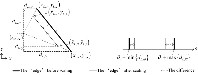
Suppose that the 𝒞 L p subscript 𝒞 𝐿 𝑝 \mathcal{C}_{Lp} m 𝑚 m E L , n + 1 , … , E L , n + m subscript 𝐸 𝐿 𝑛 1
… subscript 𝐸 𝐿 𝑛 𝑚
E_{L,n+1},...,E_{L,n+m} p L , i , i ∈ ℛ subscript 𝑝 𝐿 𝑖
𝑖
ℛ p_{L,i},i\in\mathcal{R} E L , i , i ∈ ℛ subscript 𝐸 𝐿 𝑖
𝑖
ℛ E_{L,i},i\in\mathcal{R} p L , i = [ x L , i , y L , i ] T subscript 𝑝 𝐿 𝑖
superscript subscript 𝑥 𝐿 𝑖
subscript 𝑦 𝐿 𝑖
𝑇 p_{L,i}=[x_{L,i},y_{L,i}]^{T} p L , j = [ x L , j , y L , j ] T subscript 𝑝 𝐿 𝑗
superscript subscript 𝑥 𝐿 𝑗
subscript 𝑦 𝐿 𝑗
𝑇 p_{L,j}=[x_{L,j},y_{L,j}]^{T} j = i + 1 𝑗 𝑖 1 j=i+1 i ≠ n + m 𝑖 𝑛 𝑚 i\neq n+m j = n + 1 , ∀ i ∈ ℛ formulae-sequence 𝑗 𝑛 1 for-all 𝑖 ℛ j=n+1,\forall i\in\mathcal{R} 3 E L , i subscript 𝐸 𝐿 𝑖
E_{L,i}
p L , i = [ x c ( t ) + d L , i x , y c ( t ) + d L , i y ] T , p L , j = [ x c ( t ) + d L , j x , y c ( t ) + d L , j y ] T . formulae-sequence subscript 𝑝 𝐿 𝑖
superscript subscript 𝑥 𝑐 𝑡 subscript 𝑑 𝐿 𝑖 𝑥
subscript 𝑦 𝑐 𝑡 subscript 𝑑 𝐿 𝑖 𝑦
𝑇 subscript 𝑝 𝐿 𝑗
superscript subscript 𝑥 𝑐 𝑡 subscript 𝑑 𝐿 𝑗 𝑥
subscript 𝑦 𝑐 𝑡 subscript 𝑑 𝐿 𝑗 𝑦
𝑇 \begin{split}p_{L,i}&=[x_{c}(t)+d_{L,ix},y_{c}(t)+d_{L,iy}]^{T},\\
p_{L,j}&=[x_{c}(t)+d_{L,jx},y_{c}(t)+d_{L,jy}]^{T}.\end{split} (25)
Then, the scaled coordinates of (25 η ~ L , j subscript ~ 𝜂 𝐿 𝑗
\tilde{\eta}_{L,j} 7
p ~ L , i = [ x c ( t ) + μ d L , i x , y c ( t ) + μ d L , i y ] T , p ~ L , j = [ x c ( t ) + μ d L , j x , y c ( t ) + μ d L , j y ] T . formulae-sequence subscript ~ 𝑝 𝐿 𝑖
superscript subscript 𝑥 𝑐 𝑡 𝜇 subscript 𝑑 𝐿 𝑖 𝑥
subscript 𝑦 𝑐 𝑡 𝜇 subscript 𝑑 𝐿 𝑖 𝑦
𝑇 subscript ~ 𝑝 𝐿 𝑗
superscript subscript 𝑥 𝑐 𝑡 𝜇 subscript 𝑑 𝐿 𝑗 𝑥
subscript 𝑦 𝑐 𝑡 𝜇 subscript 𝑑 𝐿 𝑗 𝑦
𝑇 \begin{split}\tilde{p}_{L,i}&=[x_{c}(t)+\mu d_{L,ix},y_{c}(t)+\mu d_{L,iy}]^{T},\\
\tilde{p}_{L,j}&=[x_{c}(t)+\mu d_{L,jx},y_{c}(t)+\mu d_{L,jy}]^{T}.\end{split} (26)
We denote the edge connected by p ~ L , i subscript ~ 𝑝 𝐿 𝑖
\tilde{p}_{L,i} p ~ L , j subscript ~ 𝑝 𝐿 𝑗
\tilde{p}_{L,j} E ~ L , i subscript ~ 𝐸 𝐿 𝑖
\tilde{E}_{L,i} ( E L , i , E ~ L , i ) subscript 𝐸 𝐿 𝑖
subscript ~ 𝐸 𝐿 𝑖
(E_{L,i},\tilde{E}_{L,i}) 25 26
‖ p L , i − p L , j ‖ = μ ‖ p ~ L , i − p ~ L , j ‖ , norm subscript 𝑝 𝐿 𝑖
subscript 𝑝 𝐿 𝑗
𝜇 norm subscript ~ 𝑝 𝐿 𝑖
subscript ~ 𝑝 𝐿 𝑗
\left\|{{p_{L,i}}-{p_{L,j}}}\right\|=\mu\left\|{{{\tilde{p}}_{L,i}}-{{\tilde{p}}_{L,j}}}\right\|, (27)
which means that the length of edge E L , i subscript 𝐸 𝐿 𝑖
E_{L,i} E ~ L , i subscript ~ 𝐸 𝐿 𝑖
\tilde{E}_{L,i} μ 𝜇 \mu m 𝑚 m ( E L , i , E ~ L , i ) , ∀ i ∈ ℛ subscript 𝐸 𝐿 𝑖
subscript ~ 𝐸 𝐿 𝑖
for-all 𝑖
ℛ (E_{L,i},\tilde{E}_{L,i}),\forall i\in\mathcal{R} p ~ L , i , ∀ i ∈ ℛ subscript ~ 𝑝 𝐿 𝑖
for-all 𝑖
ℛ \tilde{p}_{L,i},\forall i\in\mathcal{R} 𝒞 ~ L p subscript ~ 𝒞 𝐿 𝑝 \tilde{\mathcal{C}}_{Lp} 𝒞 L p subscript 𝒞 𝐿 𝑝 \mathcal{C}_{Lp} 3 0 < μ < 1 0 𝜇 1 0<\mu<1 𝒞 ~ L p subscript ~ 𝒞 𝐿 𝑝 \tilde{\mathcal{C}}_{Lp} 𝒞 L p subscript 𝒞 𝐿 𝑝 \mathcal{C}_{Lp} 𝒞 ~ L p ⊆ 𝒞 L p subscript ~ 𝒞 𝐿 𝑝 subscript 𝒞 𝐿 𝑝 \tilde{\mathcal{C}}_{Lp}\subseteq\mathcal{C}_{Lp} 𝒞 ~ L θ subscript ~ 𝒞 𝐿 𝜃 \tilde{\mathcal{C}}_{L\theta} 𝒞 ~ L θ = { θ ∈ ℝ | θ ∈ [ θ c ( t ) + μ min { d L , j θ } , θ c ( t ) + μ max { d L , j θ } ] , ∀ j ∈ ℛ } subscript ~ 𝒞 𝐿 𝜃 conditional-set 𝜃 ℝ formulae-sequence 𝜃 subscript 𝜃 𝑐 𝑡 𝜇 subscript 𝑑 𝐿 𝑗 𝜃
subscript 𝜃 𝑐 𝑡 𝜇 subscript 𝑑 𝐿 𝑗 𝜃
for-all 𝑗 ℛ \tilde{\mathcal{C}}_{L\theta}=\{\theta\in\mathbb{R}|\theta\in[\theta_{c}(t)+\mu\min\{d_{L,j\theta}\},\theta_{c}(t)+\mu\max\{{d}_{L,j\theta}\}],\forall j\in\mathcal{R}\} 𝒞 ~ L θ ⊆ 𝒞 L θ subscript ~ 𝒞 𝐿 𝜃 subscript 𝒞 𝐿 𝜃 \tilde{\mathcal{C}}_{L\theta}\subseteq\mathcal{C}_{L\theta}
To prove the property 2, we calculate the straight-line equations of paired edges E L , i subscript 𝐸 𝐿 𝑖
E_{L,i} E ~ L , i subscript ~ 𝐸 𝐿 𝑖
\tilde{E}_{L,i}
( d L , j y − d L , i y ) x + ( d L , i x − d L , i y ) y + [ x c ( t ) + d L , j x ] [ y c ( t ) + d L , i y ] − [ x c ( t ) + d L , i x ] [ y c ( t ) + d L , j y ] = 0 ; subscript 𝑑 𝐿 𝑗 𝑦
subscript 𝑑 𝐿 𝑖 𝑦
𝑥 subscript 𝑑 𝐿 𝑖 𝑥
subscript 𝑑 𝐿 𝑖 𝑦
𝑦 delimited-[] subscript 𝑥 𝑐 𝑡 subscript 𝑑 𝐿 𝑗 𝑥
delimited-[] subscript 𝑦 𝑐 𝑡 subscript 𝑑 𝐿 𝑖 𝑦
delimited-[] subscript 𝑥 𝑐 𝑡 subscript 𝑑 𝐿 𝑖 𝑥
delimited-[] subscript 𝑦 𝑐 𝑡 subscript 𝑑 𝐿 𝑗 𝑦
0 \begin{split}&(d_{L,jy}-d_{L,iy})x+(d_{L,ix}-d_{L,iy})y+[x_{c}(t)+d_{L,jx}][y_{c}(t)+d_{L,iy}]-[x_{c}(t)+d_{L,ix}][y_{c}(t)+d_{L,jy}]=0;\end{split} (28a)
μ ( d L , j y − d L , i y ) x + μ ( d L , i x − d L , i y ) y + [ x c ( t ) + μ d L , j x ] [ y c ( t ) + μ d L , i y ] − [ x c ( t ) + μ d L , i x ] [ y c ( t ) + μ d L , j y ] = 0 . 𝜇 subscript 𝑑 𝐿 𝑗 𝑦
subscript 𝑑 𝐿 𝑖 𝑦
𝑥 𝜇 subscript 𝑑 𝐿 𝑖 𝑥
subscript 𝑑 𝐿 𝑖 𝑦
𝑦 delimited-[] subscript 𝑥 𝑐 𝑡 𝜇 subscript 𝑑 𝐿 𝑗 𝑥
delimited-[] subscript 𝑦 𝑐 𝑡 𝜇 subscript 𝑑 𝐿 𝑖 𝑦
delimited-[] subscript 𝑥 𝑐 𝑡 𝜇 subscript 𝑑 𝐿 𝑖 𝑥
delimited-[] subscript 𝑦 𝑐 𝑡 𝜇 subscript 𝑑 𝐿 𝑗 𝑦
0 \begin{split}&\mu(d_{L,jy}-d_{L,iy})x+\mu(d_{L,ix}-d_{L,iy})y+[x_{c}(t)+\mu d_{L,jx}][y_{c}(t)+\mu d_{L,iy}]-[x_{c}(t)+\mu d_{L,ix}][y_{c}(t)+\mu d_{L,jy}]=0.\end{split} (28b)
Obviously, the straight lines described by (28a 28b E L , i subscript 𝐸 𝐿 𝑖
E_{L,i} E ~ L , i subscript ~ 𝐸 𝐿 𝑖
\tilde{E}_{L,i} E L , i subscript 𝐸 𝐿 𝑖
E_{L,i} E ~ L , i subscript ~ 𝐸 𝐿 𝑖
\tilde{E}_{L,i}
dis ( E L , i , E ~ L , i ) = ( 1 − μ ) | d L , j x d L , i y − d L , i x d L , j y | ( d L , j y − d L , i y ) 2 + ( d L , i x − d L , i y ) 2 , dis subscript 𝐸 𝐿 𝑖
subscript ~ 𝐸 𝐿 𝑖
1 𝜇 subscript 𝑑 𝐿 𝑗 𝑥
subscript 𝑑 𝐿 𝑖 𝑦
subscript 𝑑 𝐿 𝑖 𝑥
subscript 𝑑 𝐿 𝑗 𝑦
superscript subscript 𝑑 𝐿 𝑗 𝑦
subscript 𝑑 𝐿 𝑖 𝑦
2 superscript subscript 𝑑 𝐿 𝑖 𝑥
subscript 𝑑 𝐿 𝑖 𝑦
2 \mathrm{dis}(E_{L,i},\tilde{E}_{L,i})=(1-\mu)\frac{|d_{L,jx}d_{L,iy}-d_{L,ix}d_{L,jy}|}{\sqrt{(d_{L,jy}-d_{L,iy})^{2}+(d_{L,ix}-d_{L,iy})^{2}}}, (29)
where ‘dis’ means ‘the distance of’. Note that the Assumption 3 29 dis ( E L , i , E ~ L , i ) > 0 dis subscript 𝐸 𝐿 𝑖
subscript ~ 𝐸 𝐿 𝑖
0 \mathrm{dis}(E_{L,i},\tilde{E}_{L,i})>0
α p = ( 1 − μ ) min { | d L , j x d L , i y − d L , i x d L , j y | ( d L , j y − d L , i y ) 2 + ( d L , i x − d L , i y ) 2 } , ∀ i , j ∈ ℛ . formulae-sequence subscript 𝛼 𝑝 1 𝜇 subscript 𝑑 𝐿 𝑗 𝑥
subscript 𝑑 𝐿 𝑖 𝑦
subscript 𝑑 𝐿 𝑖 𝑥
subscript 𝑑 𝐿 𝑗 𝑦
superscript subscript 𝑑 𝐿 𝑗 𝑦
subscript 𝑑 𝐿 𝑖 𝑦
2 superscript subscript 𝑑 𝐿 𝑖 𝑥
subscript 𝑑 𝐿 𝑖 𝑦
2 for-all 𝑖
𝑗 ℛ \alpha_{p}=(1-\mu)\min\left\{\frac{|d_{L,jx}d_{L,iy}-d_{L,ix}d_{L,jy}|}{\sqrt{(d_{L,jy}-d_{L,iy})^{2}+(d_{L,ix}-d_{L,iy})^{2}}}\right\},\forall i,j\in\mathcal{R}. (30)
The constant α p subscript 𝛼 𝑝 \alpha_{p} E L , i subscript 𝐸 𝐿 𝑖
E_{L,i} E ~ L , i , ∀ i ∈ ℛ subscript ~ 𝐸 𝐿 𝑖
for-all 𝑖
ℛ \tilde{E}_{L,i},\forall i\in\mathcal{R} 𝒞 ~ L p subscript ~ 𝒞 𝐿 𝑝 \tilde{\mathcal{C}}_{Lp} 𝒞 L p subscript 𝒞 𝐿 𝑝 \mathcal{C}_{Lp} α p subscript 𝛼 𝑝 \alpha_{p} α θ subscript 𝛼 𝜃 \alpha_{\theta}
α θ = ( 1 − μ ) min { | d L , j θ | } , ∀ j ∈ ℛ . formulae-sequence subscript 𝛼 𝜃 1 𝜇 subscript 𝑑 𝐿 𝑗 𝜃
for-all 𝑗 ℛ \alpha_{\theta}=(1-\mu)\min\left\{|d_{L,j\theta}|\right\},\forall j\in\mathcal{R}. (31)
A graphical version of the above analysis refers to Fig. 2. The choice of α p subscript 𝛼 𝑝 \alpha_{p} α θ subscript 𝛼 𝜃 \alpha_{\theta}
Figure 1: Illustration of constructing the convex sub-hulls.
By the expressions of (30 31 α p subscript 𝛼 𝑝 \alpha_{p} α θ subscript 𝛼 𝜃 \alpha_{\theta} μ 𝜇 \mu 𝒞 ~ L p subscript ~ 𝒞 𝐿 𝑝 \tilde{\mathcal{C}}_{Lp} 𝒞 ~ L θ subscript ~ 𝒞 𝐿 𝜃 \tilde{\mathcal{C}}_{L\theta} p F , i − p F , i r subscript 𝑝 𝐹 𝑖
subscript 𝑝 𝐹 𝑖 𝑟
p_{F,i}-p_{F,ir} θ F , i − θ F , i r subscript 𝜃 𝐹 𝑖
subscript 𝜃 𝐹 𝑖 𝑟
\theta_{F,i}-\theta_{F,ir}