A Unifying Bayesian Approach for Sample Size Determination Using Design and Analysis Priors

Abstract

Power and sample size analysis comprises a critical component of clinical trial study design. There is an extensive collection of methods addressing this problem from diverse perspectives. The Bayesian paradigm, in particular, has attracted noticeable attention and includes different perspectives for sample size determination. Building upon a cost-effectiveness analysis undertaken by O’Hagan and Stevens, (2001) with different priors in the design and analysis stage, we develop a general Bayesian framework for simulation-based sample size determination that can be easily implemented on modest computing architectures. We further qualify the need for different priors for the design and analysis stage. We work primarily in the context of conjugate Bayesian linear regression models, where we consider the situation with known and unknown variances. Throughout, we draw parallels with frequentist solutions, which arise as special cases, and alternate Bayesian approaches with an emphasis on how the numerical results from existing methods arise as special cases in our framework.

Keywords: Bayesian and classical inference; Bayesian assurance; clinical trials; power; sample size.

1 Introduction

A crucial problem in experimental design is that of determining the sample size for a proposed study. There is, by now, a substantial literature in classical and Bayesian settings. Classical sample size calculations have been treated in depth in texts such as Kraemer and Thiemann, (1987), Cohen, (1988), and Desu and Raghavarao, (1990), while extensions to linear and generalized linear models have been addressed in Self and Mauritsen, (1988), Self et al., (1992), Muller et al., (1992) and Liu and Liang, (1997). The Bayesian setting has also allocated a decent amount of attention towards sample size determination. A widely referenced issue of The Statistician (vol. 46, issue 2, 1997) includes a number of articles from different perspectives (see, e.g., the articles by Lindley,, 1997; Pham-Gia,, 1997; Adcock,, 1997; Joseph et al.,, 1997). Within the Bayesian setting itself, there have been efforts to distinguish between a formal utility approach (Raiffa and Schlaifer,, 1961; Berger,, 1985; Lindley,, 1997; Müller and Parmigiani,, 1995) and approaches that attempt to determine sample size based upon some criterion of analysis or model performance (Rahme et al.,, 2000; Gelfand and Wang,, 2002; O’Hagan and Stevens,, 2001). Other proposed solutions adopt a more tailored approach. For example, Ibrahim et al., (2012) specifically target Bayesian meta-experimental design using survival regression models; Reyes and Ghosh, (2013) propose a framework based on Bayesian average errors capable of simulatenously controlling for Type I and Type II errors, while Joseph et al., (1997) rely on lengths of posterior credible intervals to gauge their sample size estimates.

The aforementioned literature presents the problem in a variety of applications including, but not limited to, clinical trials. Bayesian treatments specific to clinical trials can be found in Spiegelhalter et al., (1993), Parmigiani, (2002), Berry, (2006), Berry et al., (2010), Lee and Zelen, (2000), and Lee and Chu, (2012). Regardless of the specific approach, all of the cited articles above address the sample size problem based on some well-defined objective that is desired in the analysis stage. The design of the study, therefore, should consider that the analysis objective is met with a certain probability. The framework we develop here is built upon this simple idea. A clear analysis objective and proper sampling execution are all that is needed to provide us with the necessary sample size.

1.1 Classical Power and Sample Size

The classical power and sample size analysis problem in the frequentist setting is widely applied in diverse settings. For example, we can formulate a hypothesis concerning the population mean. A one-sided hypothesis test for the null $\displaystyle H_{0}:\theta=\theta_{0}$ against the alternative $H_{a}:\theta>\theta_{0}$, where $\theta$ is the population mean, is decided on the location of $\theta_{0}$ with respect to the distribition of the sample mean $\bar{y}$. Assuming a known value for the population variance $\sigma^{2}$ and that the sample mean’s distribition is (approximately) Gaussian, we reject $H_{0}$ if $\bar{y}>\theta_{0}+\frac{\sigma}{\sqrt{n}}Z_{1-\alpha}$, where $\alpha$ is the specified Type-I error and $Z_{1-\alpha}$ is the corresponding quantile of the Gaussian distribution. The statistical “power” of the test is $1-\beta$, where $\beta=P(\mbox{Rej }H_{0}\,|\,H_{a})$ is the Type-II error. Straightforward algebra yields the ubiquitous sample size formula, $\displaystyle n=(Z_{\alpha}+Z_{\beta})^{2}\left(\frac{\sigma}{\Delta}\right)^{2}$, derived from the power:

$$1-\beta=P\left(\bar{y}>\theta_{0}+\frac{\sigma}{\sqrt{n}}Z_{1-\alpha}\,|\,\theta=\theta_{1}\right)=\Phi\left(\sqrt{n}\frac{\Delta}{\sigma}+Z_{\alpha}\right),$$ (1)

where $\Delta=\theta_{1}-\theta_{0}$ is the critical difference. Given any fixed value of $\Delta/\sigma$, the power curve is a function of sample size and can be plotted as in Figure 1. The sample size required to achieve a specified power can then be read from the power curve.

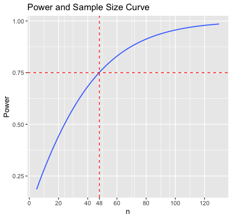
Figure 1: Power curve example. Dotted lines indicate how a sample size of 34 is required to achieve a power of 0.75.

More generally, power curves, such as the one shown in Figure 1, may not be available in closed form but can be simulated for different sample sizes. They quantify our degree of assurance regarding our ability to meet our analysis objective (rejecting the null) for different sample sizes. Formulating sample size determination as a decision problem so that power is an increasing function of sample size, offers the investigator a visual aid in helping deduce the minimum sample size needed to achieve a desired power.

1.2 Bayesian Assurance

From a Bayesian standpoint, there is no need to condition on a fixed alternative. Instead, we determine the tenability of a hypothesis given the data we observe. A joint probability model is constructed for the parameters and the data using a prior distribition for the parameters and the likelihood function of the data conditional on the parameters. Inference proceeds from the posterior distribition of the parameters given the data.

In the design stage we have not observed the data. Therefore, we will need to formulate a data generating mechanism and, subsequently, consider the posterior distribution given the realized data to evaluate the tenability of a hypothesis regarding our parameter. We then use the probability law associated with the data generating mechanism to assign a degree of assurance of our analysis objective. As a sufficiently simple example, consider a situation where we seek to evaluate the tenability of $H:\theta>\theta_{0}$ given data from a Gaussian population with mean $\theta$ and a known variance $\sigma^{2}$. Assuming the prior $\theta\sim N\left(\theta_{1},\frac{\sigma^{2}}{n_{0}}\right)$, where $n_{0}$ reflects the precision of the prior relative to the data, and the likelihood of the sample mean $\displaystyle\bar{y}\sim N\left(\theta,\frac{\sigma^{2}}{n}\right)$, the posterior distribution of $\theta$ can then be obtained by multiplying the prior and the likelihood as

$$N\left(\theta{\left|\theta_{1},\frac{\sigma^{2}}{n_{0}}\right.}\right)\times N\left(\bar{y}{\left|\theta,\frac{\sigma^{2}}{n}\right.}\right)\propto N\left(\theta{\left|\frac{n_{0}}{n+n_{0}}\theta_{1}+\frac{n}{n+n_{0}}\bar{y},\frac{\sigma^{2}}{n+n_{0}}\right.}\right)\;.$$ (2)

Our analysis objective is to ascertain whether $P(\theta>\theta_{0}\,|\,\bar{y})>1-\alpha$, where $\alpha$ is a fixed number. The posterior distribution in (2) gives us $P(\theta>\theta_{0}\,|\,\bar{y})$ and we define

$$\delta=P_{\bar{y}}\left\{\bar{y}:P(\theta>\theta_{0}\,|\,\bar{y})>1-\alpha\right\}$$ (3)

as a Bayesian counterpart of statistical power, which we refer to as Bayesian assurance. The inner probability defines our analysis objective, while the outer probability defines our chances of meeting the analysis objective under the given data generating mechanism.

1.3 Manuscript Overview

Our current manuscript intends to explore Bayesian assurance and subsequent sample size calculations as described through (2) and (3) in the general context of conjugate Bayesian linear regression. Of particular emphasis will be the data generating mechanism and providing motivation behind quantifying separate prior beliefs at the design and analysis stage of clinical trials (O’Hagan and Stevens,, 2001). The balance of this manuscript proceeds as follows. Section 2 presents the Bayesian sample size determination problem embedded within a conjugate Bayesian linear model. This offers us analytic tractability through which we motivate the need for different prior distributions for designing and analyzing a study. Section 2.3 considers the cases of known and unknown variances and offers corresponding algorithms. Section 3 casts the cost-effectiveness problem explored by O’Hagan and Stevens, (2001) in our framework, which we revisit using known and unknown variances, and we also compare with other Bayesian alternatives for sample size calculations including for inference using proportions. We close the paper in Section 4 with additional points of discussion and future aims.

2 Bayesian Assurance and Sample Size Determination

2.1 Conjugate Bayesian Linear Regression

Consider a proposed study where a certain number, say $n$, of observations, which we denote by $y_{n}=(y_{1},y_{2}\ldots,y_{n})^{\top}$, are to be collected in the presence of $p$ controlled explanatory variables, say $x_{1},x_{2},\ldots,x_{p}$, that will be known to the investigator for any unit $i$ at the design stage. Consider the usual normal linear regression setting such that $y_{n}=X_{n}\beta+\epsilon_{n}$, where $X_{n}$ is $n\times p$ with $i$-th row corresponding to $x_{i}^{\top}$ and $\epsilon_{n}\sim N(0,\sigma^{2}V_{n})$, where $V_{n}$ is a known $n\times n$ correlation matrix. Both $X_{n}$ and $V_{n}$ are assumed known for each sample size $n$ through design and modeling considerations. A conjugate Bayesian linear regression model specifies the joint distribution of the parameters $\{\beta,\sigma^{2}\}$ and the data as

$$IG(\sigma^{2}\,|\,a_{\sigma},b_{\sigma})\times(\beta\,|\,\mu_{\beta},\sigma^{2}V_{\beta})\times N(y_{n}\,|\,X_{n}\beta,\sigma^{2}V_{n})$$ (4)

Inference proceeds from the posterior distribution derived from (4),

$$p(\beta,\sigma^{2}\,|\,y_{n}) =\underbrace{IG(\sigma^{2}\,|\,a^{*}_{\sigma},b^{*}_{\sigma})}_{p(\sigma^{2}\,|\,y_{n})}\times\underbrace{N(\beta\,|\,M_{n}m_{n},\sigma^{2}M_{n})}_{p(\beta\,|\,\sigma^{2},y_{n})}\;,$$ (5)

where $a^{*}_{\sigma}=a_{\sigma}+n/2$, $b^{*}_{\sigma}=b_{\sigma}+(1/2)\left\{\mu_{\beta}^{\top}V_{\beta}^{-1}\mu_{\beta}+y_{n}^{\top}V_{n}^{-1}y_{n}-m_{n}^{\top}M_{n}m_{n}\right\}$, $M_{n}^{-1}=V_{\beta}^{-1}+X_{n}^{\top}V_{n}^{-1}X_{n}$ and $m_{n}=V_{\beta}^{-1}\mu_{\beta}+X_{n}^{\top}V_{n}^{-1}y_{n}$. Sampling from the joint posterior distribution of $\{\beta,\sigma^{2}\}$ is achieved by first sampling $\sigma^{2}\sim IG(a^{*}_{\sigma},b^{*}_{\sigma})$ and then sampling $\beta\sim N(M_{n}m_{n},\sigma^{2}M_{n})$ for each sampled $\sigma^{2}$. This yields marginal posterior samples from $p(\beta\,|\,y_{n})$, which is a non-central multivariate $t$ distribution, though we do not need to work with its complicated density function. See Gelman et al., (2013) for further details on the conjugate Bayesian linear regression model and sampling from its posterior.

We wish to decide whether our realized data will favor $H:u^{\top}\beta>0$, where $u$ is a $p\times 1$ vector of fixed contrasts. In practice, a decision on the tenability of $H$ is often based on the $100(1-\alpha)\%$ posterior credible interval,

$$\left(u^{\top}M_{n}m_{n}-Z_{1-\alpha/2}\sigma\sqrt{u^{\top}M_{n}u},\;u^{\top}M_{n}m_{n}+Z_{1-\alpha/2}\sigma\sqrt{u^{\top}M_{n}u}\right)\;,$$ (6)

obtained from the conditional posterior predictive distribution $p(\beta\,|\,\sigma,y_{n})$. The data would favor $H$ if $y_{n}$ belongs to the following set

$$S_{\alpha}(n;y_{n},\sigma,\mu_{\beta},V_{\beta},V_{n})=\left\{y_{n}:u^{\top}M_{m}m_{n}>Z_{1-\alpha/2}\sigma\sqrt{u^{\top}M_{n}u}\right\}\;.$$

This is equivalent to $0$ being below the two-sided $100(1-\alpha)\%$ credible interval for $u^{\top}\beta$. Practical Bayesian designs will seek to assure the investigator that the above criterion will be achieved with a sufficiently high probability through the Bayesian assurance,

$$\delta(n;\sigma,u,\mu_{\beta},V_{\beta},V_{n})=P_{y_{n}}(S_{\alpha}(n;y_{n},\sigma,\mu_{\beta},V_{\beta},V_{n}))\\ =P_{y_{n}}\left\{y_{n}:u^{\top}M_{m}m_{n}>Z_{1-\alpha/2}\sigma\sqrt{u^{\top}M_{n}u}\right\}\;,$$ (7)

which generalizes the definition in (3). Given the assumptions on the model, the fixed values of the parameters $\{\mu_{\beta},V_{\beta},\sigma,V_{n}\}$ and the fixed vector $u$ that determines the hypothesis being tested, the Bayesian assurance function evaluates the probability of rejecting the null hypothesis under the marginal probability distribution of the realized data corresponding to any given sample size $n$. Choice of sample size will be determined by the smallest value of $n$ that will ensure $\delta(n;\sigma,u,\mu_{\beta},V_{\beta},V_{n})>\gamma$, where $\gamma$ is a specified number.

2.2 Limitations for a single prior

Let us consider the special case when $X_{n}=1_{n}$ so that $\beta$ is a scalar with prior distribution $\beta\sim N(\beta_{1},\sigma^{2}/n_{0})$, where $n_{0}>0$ is a fixed precision parameter (sometimes referred to as “prior sample size”), $V_{n}=I_{n}$ and $H:\beta>\beta_{0}$. We decide in favor of $H$ if the data lies in

$$S_{\alpha}(n;y,\sigma,\beta_{0},\beta_{1},n_{0})=\left\{\bar{y}:\bar{y}>\beta_{0}-\frac{n_{0}}{n}(\beta_{1}-\beta_{0})-\sqrt{\left(1+\frac{n_{0}}{n}\right)}\frac{\sigma}{\sqrt{n}}Z_{\alpha}\right\}\;,$$

where the expression on the right reveals a convenient condition in terms of the sample mean. As $n_{0}\to 0$, i.e., the prior becomes vague, $S_{\alpha}(n;y,\sigma,\beta_{0},\beta_{1},n_{0})$ collapses to the critical region in classical inference for testing $H_{0}:\beta=\beta_{0}$ against $H_{a}:\beta=\beta_{1}$. The Bayesian assurance function is

$$\delta(n;\sigma,\Delta,n_{0})=\Phi\left(\sqrt{n_{0}}\left[\sqrt{1+\frac{n_{0}}{n}}\left(\frac{\Delta}{\sigma}\right)+Z_{\alpha}\sqrt{\frac{1}{n}}\right]\right)\;,$$ (8)

where $\Delta=\beta_{1}-\beta_{0}$. Given $n_{0}$, we will compute the sample size needed to detect a critical difference of $\Delta$ with probability $1-\beta$ as $n=\arg\min\{n:\delta(\Delta,n)\geq 1-\beta\}$. However, the limiting properties of the function in (8) are not without problems. When the prior is vague, i.e., $n_{0}\to 0$, then

$$\lim_{n_{0}\to 0}\delta(\Delta,n)=\Phi\left(0\right)=0.5\;,$$

while in the case when the prior is precise, i.e., $n_{0}\to\infty$ we obtain

$$\lim_{n_{0}\to\infty}\delta(\Delta,n)=\left\{\begin{array}[]{ll}1&\mbox{if $\Delta>0$}\\ 0&\mbox{if $\Delta\leq 0$}\\ \end{array}\right..$$ (9)

This is undesirable. Vague priors are customary in Bayesian analysis, but they propagate enough uncertainty that the marginal distribution of the data under the given model will force the assurance to be lower than 0.5. In other words, regardless of how large a sample size we have, we cannot assure the investigator with probability greater than 50% that the null hypothesis will be rejected. At the other extreme, where the prior is fully precise, it fully dominates the data (or the likelihood) and there is no information from the data that is used in the decision. Therefore, the assurance is a function of the prior only and we will always or never reject the null hypothesis depending upon whether $\Delta>0$ or $\Delta<0$.

In order to resolve this issue, we work with two different sets of priors, one at the design stage and another at the analysis stage. Building upon O’Hagan and Stevens (2001), we elucidate with the Bayesian linear regression model in the next section and offer a simulation-based framework for computing the Bayesian assurance curves.

2.3 Bayesian Assurance Using Design and Analysis Priors

We consider two scenarios that are driven by the amount of information given in a study. We develop the corresponding algorithms based on these assumptions. The first case assumes that the population variance $\sigma^{2}$ is known and the second case assumes $\sigma^{2}$ is unknown, prompting us to consider additional prior distributrions for $\sigma^{2}$ in the design and analysis stage. Our context remains testing the tenability of $H:u^{\top}\beta>C$ given realized data from a study, where $C$ is a known constant.

2.3.1 Known Variance $\sigma^{2}$

If $\sigma^{2}$ is known and fixed, then the posterior distribution of $\beta$ is $\displaystyle p(\beta\,|\,\sigma^{2},y_{n})=N(\beta|M_{n}m_{n},\sigma^{2}M_{n})$ as shown in Equation 5. Hence, standardization leads to

$$\left.\frac{u^{\top}\beta-u^{\top}M_{n}m_{n}}{\sigma\sqrt{u^{\top}M_{n}u}}\right|\sigma^{2},y_{n}\sim N(0,1)\;.$$ (10)

To evaluate the credibility of $H:u^{\top}\beta>C$, where $u$ denotes a known $p\times 1$ vector and $C$ is a known constant, we decide in favor of $H$ if the observed data belongs in the region:

$$A_{\alpha}(u,\beta,C) =\left\{y_{n}:P\left(u^{\top}\beta\leq C|y_{n}\right)<\alpha\right\}=\left\{y_{n}:\Phi\left(\frac{C-u^{\top}M_{n}m_{n}}{\sigma\sqrt{u^{\top}M_{n}u}}\right)<\alpha\right\}.$$

Given the data $y_{n}$ and the fixed parameters in the analysis priors, we can evaluate $M_{n}$ and $m_{n}$ and hence, for any given $\sigma$, $C$ and $\alpha$, ascertain if we have credibility for $H$ or not.

In the design objective we need to ask ourselves “What sample size is needed to assure us that the analysis objective is met $100\gamma\%$ of the time?” Therefore, we seek $n$ so that

$$\delta(n) =P_{y_{n}}(A_{\alpha}(u,\beta,C))=P_{y_{n}}\left\{y_{n}:\Phi\left(\frac{C-u^{\top}M_{n}m_{n}}{\sigma\sqrt{u^{\top}M_{n}u}}\right)<\alpha\right\}\geq\gamma\;,$$ (11)

where $\delta(n)$ is the Bayesian assurance. In order to evaluate (11), we will need the marginal distribution of $y_{n}$. In light of the paradox in (9), our belief about the population from which our sample will be taken is quantified using the design priors. Therefore, the “marginal” distribution of $y_{n}$ under the design prior will be derived from

$$y_{n} =X_{n}\beta+e_{n};\quad e_{n}\sim N(0,\sigma^{2}V_{n})\;;\quad\beta=\mu_{\beta}^{(d)}+\omega;\quad\omega\sim N(0,\sigma^{2}V_{\beta}^{(d)})\;,$$ (12)

where $\beta\sim N(\mu_{\beta}^{(d)},\sigma^{2}V_{\beta}^{(d)})$ is the design prior on $\beta$. Substituting the equation for $\beta$ into the equation for $y_{n}$ in (12) gives $y_{n}=X\mu_{\beta}^{(d)}+(X\omega+e_{n})$ and, hence, $y_{n}\sim N\left(X\mu_{\beta}^{(d)},\sigma^{2}V_{n}^{*}\right)$, where $V_{n}^{\ast}=\left(XV_{\beta}^{(d)}X^{\top}+V_{n}\right)$. We now have a simulation strategy to estimate our Bayesian assurance. We fix sample size $n$ and generate a sequence of $J$ data sets $y_{n}^{(1)},y_{n}^{(2)},\ldots,y_{n}^{(J)}$, each of size $n$ from $N\left(X\mu_{\beta}^{(d)},\sigma^{2}V_{n}^{*}\right)$. Then, a Monte Carlo estimate of the Bayesian assurance is

$$\hat{\delta}(n)=\frac{1}{J}\sum_{j=1}^{J}\mathbb{I}\left(\left\{y_{n}^{(j)}:\Phi\left(\frac{C-u^{\top}M_{n}^{(j)}m_{n}^{(j)}}{\sigma\sqrt{u^{\top}M_{n}^{(j)}u}}\right)<\alpha\right\}\right)\;,$$ (13)

where $\mathbb{I}(\cdot)$ is the indicator function of the event in its argument, $M_{n}^{(j)}$ and $m_{n}^{(j)}$ are the values of $M_{n}$ and $m_{n}$ computed from $y_{n}^{(j)}$. We repeat the steps needed to compute (13) for different values of $n$ and obtain a plot of $\delta(n)$ against $n$. Our desired sample size is the smallest $n$ for which $\hat{\delta}(n)\geq\gamma$, where we seek assurance of a $100\gamma\%$ chance of deciding in favor of $H$.

A special case of the model can be considered where $X_{n}=1_{n}$ is an $n\times 1$ vector of ones, $\beta$ is a scalar, $V_{n}=I_{n}$ and we wish to evaluate the credibility of $H:\beta>\beta_{0}$. We assume $\beta\sim N(\beta_{1},\sigma^{2}/n_{a})$ in the analysis stage and $\beta\sim N(\beta_{1},\sigma^{2}/n_{d})$ in the design stage, where $\beta_{1}>\beta_{0}$. The data will favor $H$ if the sample mean lies in $A_{\alpha}(\beta_{0},\beta_{1})$, where

$$A_{\alpha}(\beta_{0},\beta_{1})=\left\{\bar{y}:\bar{y}>\beta_{0}-\frac{n_{a}}{n}(\beta_{1}-\beta_{0})-\sqrt{\left(1+\frac{n_{a}}{n}\right)}\frac{\sigma}{\sqrt{n}}Z_{\alpha}\right\}\;.$$

Using the design prior, we obtain the marginal distribution $\displaystyle\bar{y}\sim N\left(\beta_{1},\left(\frac{1}{n}+\frac{1}{n_{d}}\right)\sigma^{2}\right)$. We use this distribution to calculate $\delta(n)=P_{\bar{y}}\{\bar{y}:P(\theta<\theta_{0}\,|\,\bar{y})<\alpha\}$, which produces a closed-form expression for Bayesian assurance:

$$\delta(\Delta,n,n_{a},n_{d})=\Phi\left(\sqrt{\frac{nn_{d}}{n+n_{d}}}\left[\frac{n+n_{a}}{n}\frac{\Delta}{\sigma}+Z_{\alpha}\frac{\sqrt{n+n_{a}}}{n}\right]\right)\;,$$ (14)

where $\Delta=\beta_{1}-\beta_{0}$. As $n_{d}\to\infty$ and $n_{a}\to 0$, we obtain that

$$\lim_{n_{a}\to 0,n_{d}\to\infty}=\Phi\left(\sqrt{n}\frac{\Delta}{\sigma}+Z_{\alpha}\right)\;,$$

which is precisely the frequentist power curve. Therefore, the frequentist sample size emerges as a special case of the Bayesian sample size when the design prior becomes perfectly precise and the analysis prior becomes perfectly uninformative. Algorithm 1 presents a pseudocode to compute Bayesian assurance.

Algorithm 1 Bayesian assurance algorithm for known variance

1:procedure bayes sim($n$, $u$, $C$, $X$, $V_{n}$, $V_{\beta}^{(d)}$, $V_{\beta}^{-1(a)}$, $\mu_{\beta}^{(d)}$, $\mu_{\beta}^{(a)}$, $\sigma^{2}$, $\alpha$)

2:     count = $0$ $\triangleright$ keeps track of iterations satisfying the analysis objective

3:

4:     for $i$ in range $1$ : max number of iterations do

5:         Design Stage Starts

6:         $y\leftarrow$ Vector of $n$ values each generated from N$(X\mu_{\beta}^{(d)},\sigma^{2}(XV_{\beta}^{(d)}X^{\top}+V_{n}))$

7:         Design Stage Ends

8:

9:         Analysis Stage Starts $\triangleright$ Computes parameters of the $\beta$ posterior:

10:         $M\leftarrow(V_{\beta}^{-1(a)}+X^{\top}V_{n}^{-1}X)^{-1}$

11:         $m\leftarrow V_{\beta}^{-1(a)}\mu_{\beta}^{(a)}+X^{\top}V_{n}^{-1}y$

12:         if $\frac{C-u^{\top}Mm}{\sigma\sqrt{u^{\top}Mu}}<Z_{\alpha}$ then

13:              $Z_{i}\leftarrow 1$

14:         else

15:              if $\frac{C-u^{\top}Mm}{\sigma\sqrt{u^{\top}Mu}}\geq Z_{\alpha}$ then

16:                  $Z_{i}\leftarrow 0$

17:              end if

18:         end if

19:

20:         count $\leftarrow$ count + $Z_{i}$

21:         Analysis Stage Ends

22:     end for

23:

24:     assurance $\leftarrow$ count / max number of iterations

25:return assurance

26:

27:end procedure

2.3.2 Unknown Variance $\sigma^{2}$

When $\sigma^{2}$ is unknown, the posterior distribution of interest is $p(\beta,\sigma^{2}\,|\,y_{n})$ as opposed to the original $p(\beta\,|\,\sigma^{2},y_{n})$ delineated in the known variance case. Since $\sigma^{2}$ is no longer fixed, it becomes challenging to define a closed form condition that is capable of evaluating the credibility of $H:u^{\top}\beta>C$. Hence, we do not obtain a condition similar to (10). However, our region of interest corresponding to our analysis objective still remains as $A_{\alpha}(u,\beta,C)=\left\{y_{n}:P\left(u^{\top}\beta\leq C\,|\,y_{n}\right)<\alpha\right\}$ when deciding whether or not we are in favor of $H$. To implement this in a simulation setting, we rely on iterative sampling for both $\beta$ and $\sigma^{2}$ to estimate the assurance. We specify analysis priors $\beta\,|\,\sigma^{2}\sim N(\mu_{\beta}^{(a)},\sigma^{2}V_{\beta}^{(a)})$ and $\sigma^{2}\sim IG(a^{(a)},b^{(a)})$, where the superscripts $(a)$ signify analysis priors.

We had previously derived the posterior distribution of $\beta$ in Section 2.3.1 expressed as $p(\beta\,|\,y_{n},\sigma^{2})=N(\beta\,|\,M_{n}m_{n},\sigma^{2}M_{n})$, where $M_{n}=(V_{\beta}^{-1(a)}+X^{\top}V_{n}^{-1}X)^{-1}$ and $m_{n}=V_{\beta}^{-1(a)}\mu_{\beta}^{(a)}+X^{\top}V_{n}^{-1}y_{n}$. The posterior distribution of $\sigma^{2}$ is obtained by integrating out $\beta$ from the joint posterior distribution of $\{\beta,\sigma^{2}\}$, which yields

$$\begin{split}p(\sigma^{2}\,|\,y_{n})&\propto IG(\sigma^{2}\,|\,a^{(a)},b^{(a)})\times\int N(\beta\,|\,\mu_{\beta},\sigma^{2}V_{\beta})\times N(y_{n}\,|\,X\beta,\sigma^{2}V_{n})d\beta\\ &\propto\left(\frac{1}{\sigma^{2}}\right)^{a^{(a)}+\frac{n}{2}+1}\exp\left\{-\frac{1}{\sigma^{2}}\left(b^{(a)}+\frac{c^{\ast}}{2}\right)\right\}\;.\end{split}$$ (15)

Therefore, $p(\sigma^{2}\,|\,y_{n})=IG\left(\sigma^{2}\,|\,a^{\ast},b^{\ast}\right)$, where $a^{\ast}=a^{(a)}+\frac{n}{2}$ and $b^{\ast}=b^{(a)}+\frac{c^{\ast}}{2}=b^{(a)}+\frac{1}{2}\left\{\mu_{\beta}^{\top(a)}V_{\beta}^{-1(a)}\mu_{\beta}^{(a)}+y_{n}^{\top}V_{n}^{-1}y_{n}-m_{n}^{\top}M_{n}m_{n}\right\}$.

Recall the design stage objective aims to identify sample size $n$ that is needed to attain the assurance level specified by the investigator. Similar to Section 2.3.1 we will need the marginal distribution of $y_{n}$ with priors placed on both $\beta$ and $\sigma^{2}$. We denote these design priors as $\beta^{(d)}$ and $\sigma^{2(d)}$, respectively, to signify that we are working within the design stage. Derivation steps are almost identical to those outlined in Equation (12) for the known $\sigma^{2}$ case. With $\sigma^{2(d)}$ now treated as an unknown parameter, the marginal distribution of $y_{n}$, given $\sigma^{2(d)}$, under the design prior is derived from $y_{n}=X_{n}\beta^{(d)}+e_{n}$, $e_{n}\sim N(0,\sigma^{2(d)}V_{n})$, $\beta^{(d)}=\mu_{\beta}^{(d)}+\omega;\quad\omega\sim N(0,\sigma^{2(d)}V_{\beta}^{(d)})$, where $\beta^{(d)}\sim N(\mu_{\beta}^{(d)},\sigma^{2(d)}V_{\beta}^{(d)})$ and $\sigma^{2(d)}\sim IG(a^{(d)},b^{(d)})$. Substituting $\beta^{(d)}$ into $y_{n}$ gives us $y_{n}=X_{n}\mu_{\beta}^{(d)}+(X_{n}\omega+e_{n})$ such that $X_{n}\omega+e_{n}\sim N(0,\sigma^{2(d)}(V_{n}+X_{n}V_{\beta}^{(d)}X_{n}^{\top}))$. The marginal distribution of $p(y_{n}\,|\,\sigma^{2(d)})$ is

$$y_{n}\,|\,\sigma^{2(d)}\sim N(X_{n}\mu_{\beta}^{(d)},\sigma^{2(d)}V_{n}^{*});\quad V_{n}^{*}=X_{n}V_{\beta}^{(d)}X_{n}^{\top}+V_{n}.$$ (16)

Equation (16) specifies our data generation model for ascertaining sample size.

The pseudocode in Algorithm 2 evaluates Bayesian assurance. Each iteration comprises the design stage, where the data is generated, and an analysis stage where the data is analyzed to ascertain whether a decision favorable to the hypothesis has been made. In the design stage, we draw $\sigma^{2(d)}$ from $IG(a_{\sigma}^{(d)},b_{\sigma}^{(d)})$ and generate the data from our sampling distribution from (16), $y_{n}\sim N(X\mu_{\beta}^{(d)},\sigma^{2(d)}(XV_{\beta}^{(d)}X^{\top}+V_{n}))$. For each such data set, $\{y_{n},X_{n}\}$, we perform Bayesian inference for $\beta$ and $\sigma^{2}$. Here, we draw $J$ samples of $\beta$ and $\sigma^{2}$ from their respective posterior distributions and compute the proportion of these $J$ samples that satisfy $u^{\top}\beta_{j}>C$. If the proportion exceeds a certain threshold $1-\alpha$, then the analysis objective is met for that dataset. The above steps for the design and analysis stage are repeated for $R$ datasets and the proportion of the $R$ datasets that meet the analysis objective, i.e., deciding in favor of $H$, correspond to the Bayesian assurance.

Algorithm 2 Bayesian assurance algorithm for unknown variance

1:procedure bayes2($n$, $u$, $C$, $R$, $X$, $V_{n}$, $V_{\beta}^{(d)}$, $V_{\beta}^{-1(a)}$, $\mu_{\beta}^{(d)}$, $\mu_{\beta}^{(a)}$, $a^{(d)}$, $a^{(a)}$, $b^{(a)}$, $b^{(d)}$, $\alpha$)

2:     count1 = $0$ $\triangleright$ counts iterations that meet analysis objective

3:

4:     for $i$ in range $1:R$ do $\triangleright$ $R$ denotes number of generated datasets

5:         Begin Design Stage

6:         $\gamma^{2}\leftarrow$ IG$(a^{(d)},b^{(d)})$

7:         count2 = $0$ $\triangleright$ tracks meeting analysis objective for generated data

8:         $y\leftarrow$ $n\times 1$ vector sampled from MVN$(X\mu_{\beta}^{(d)},\gamma^{2}(XV_{\beta}^{(d)}X^{\top}+V_{n}))$

9:         End Design Stage

10:

11:         Begin Analysis Stage

12:         Compute the components that make up the posterior distributions of $\beta$ and $\sigma^{2}$:

13:         $M\leftarrow(V_{\beta}^{-1(a)}+X^{\top}V_{n}^{-1}X)^{-1}$

14:         $m\leftarrow V_{\beta}^{-1(a)}\mu_{\beta}^{(a)}+X^{\top}V_{n}^{-1}y$

15:         $a^{\ast}=a^{(a)}+\frac{n}{2}$

16:         $b^{\ast}=b^{(a)}+\frac{1}{2}\{\mu_{\beta}^{\top(a)}V_{\beta}^{-1(a)}\mu_{\beta}^{(a)}+y^{\top}V_{n}^{-1}y-m^{\top}Mm\}$

17:

18:         for $j$ in range 1:J do $\triangleright$ $J$ denotes number of posterior samples

19:              $\sigma^{2}\leftarrow$ IG($a^{\ast},b^{\ast}$)

20:              $\beta\leftarrow$ $p\times 1$ vector sampled from MVN($Mm,\sigma^{2}M$)

21:              if $u^{\top}\beta\leq C$ then

22:                  count2 $\leftarrow$ count2 + 1

23:              else

24:                  if $u^{\top}\beta>C$ then

25:                       count2 $\leftarrow$ count2

26:                  end if

27:              end if

28:         end for

29:

30:         if count2 / J $\leq\alpha$ then

31:              count1 = count1 + 1

32:         else

33:              if count2 / J $>\alpha$ then

34:                  count1 = count1

35:              end if

36:         end if

37:         End Analysis Stage

38:

39:     end for

40:     assurance $\leftarrow$ count1 / R

41:return assurance

42:

43:end procedure

3 Two-Stage Paradigm Applications

The following sections explore three existing sample size determination approaches. We show how these approaches emerge as special cases of our framework with an appropriate formulation of analysis and design stage objectives. Assurance curves are produced via simulation and pseudocodes of the algorithms are included.

3.1 Sample Size Determination in Cost-Effectiveness Setting

The first application selects a sample size based on the cost-effectiveness of new treatments undergoing Phase 3 clinical trials (O’Hagan and Stevens,, 2001). As delineated in Section 2, we construct the two-stage paradigm under the context of a conjugate linear model and generalize it to the case where the population variance $\sigma^{2}$ is unknown. We cast the example in O’Hagan and Stevens, (2001) within our framework to assess overall performance and our ability to emulate the analysis in O’Hagan and Stevens, (2001).

Consider designing a randomized clinical trial where $n_{1}$ patients are administered Treatment 1 and $n_{2}$ patients are administered Treatment 2 under some suitable model and study objectives. Let $c_{ij}$ and $e_{ij}$ denote the observed cost and efficacy values, respectively, corresponding to patient $j=1,2,\ldots,n_{i}$ receiving treatment $i$ for $i=1,2$ treatments, where $n_{i}$ is the number of patients in the $i$-th treatment group. Furthermore, the expected population mean cost efficacy under treatment $i$ are set to be $E(c_{ij})=\gamma_{j}$ and $E(c_{ij})=\mu_{i}$, respectively. The variances are taken to be $Var(c_{ij})=\tau_{i}^{2}$ and $Var(e_{ij})=\sigma_{i}^{2}$. For simplicity, we assume equal sample sizes within the treatment groups so that $n=n_{1}=n_{2}$. We also assume equal sample variances for the costs and efficacies such that $\tau^{2}$ = $\tau_{1}^{2}=\tau_{2}^{2}$ and $\sigma^{2}=\sigma_{1}^{2}=\sigma_{2}^{2}$.

O’Hagan and Stevens, (2001) utilize the net monetary benefit measure,

$$\xi=K(\mu_{2}-\mu_{1})-(\gamma_{2}-\gamma_{1}),$$ (17)

where $\gamma_{2}-\gamma_{1}$ and $\mu_{2}-\mu_{1}$ denote the true differences in costs and efficacies, respectively, between Treatment 1 and Treatment 2, and $K$ represents the maximum price that a health care provider is willing to pay in order to obtain a unit increase in efficacy, also known as the threshold unit cost. The quantity $\xi$ acts as a measure of cost-effectiveness.

Since the net monetary benefit formula expressed in Equation (17) involves assessing the cost and efficacy components conveyed within each of the two treatment groups, we set $\beta=(\mu_{1},\gamma_{1},\mu_{2},\gamma_{2})^{\top}$, where $\mu_{i}$ and $\gamma_{i}$ denote the efficacy and cost for treatments $i=1,2$. Next, we specify $y_{n}$ as a $4n\times 1$ vector consisting of $2\times 1$ vectors $y_{ij}=(c_{ij},e_{ij})^{\top}$, $i=1,2$ and $j=1,2,\ldots,n$. Each individual observation is allotted one row in the linear model. The design matrix $X_{n}$ is a $4n\times 4$ block diagonal with the $n\times 1$ vector of ones, $1_{n}$, as the blocks. With $n=n_{1}=n_{2}$, $\sigma^{2}=\sigma_{1}^{2}=\sigma_{2}^{2}$ and $\tau^{2}=\tau_{1}^{2}=\tau_{2}^{2}$, our variance matrix is $\displaystyle\sigma^{2}\underset{4n\times 4n}{V_{n}}=\sigma^{2}\begin{pmatrix}I_{n}&O&O&O\\ O&\frac{\tau^{2}}{\sigma^{2}}I_{n}&O&O\\ O&O&I_{n}&O\\ O&O&O&\frac{\tau^{2}}{\sigma^{2}}I_{n}\\ \end{pmatrix},$ where $\sigma^{2}$ is factored out to comply with our conjugate linear model formulation expressed in Equation (4).

In the analysis stage, we use the posterior distribution for $\beta$ if $\sigma^{2}$ is fixed or for $\{\beta,\sigma^{2}\}$ if $\sigma^{2}$ needs to be estimated; recall Sections 2.3.1 and 2.3.2. The posterior distribution is needed only for the analysis stage, hence it is computed using the analysis priors. Since there is no data in the design stage, there is no posterior distribution. We use the design priors as specifications for the population from which the data is generated. That is, the design priors yield the sampling distribution $y_{n}\,|\,\sigma^{2(d)}$. O’Hagan and Stevens, (2001) define $\mu_{\beta}^{(d)}=(5,6000,6.5,7200)^{\top}$ and $\displaystyle V_{\beta}^{(d)}=\begin{pmatrix}4&0&3&0\\ 0&10^{7}&0&0\\ 3&0&4&0\\ 0&0&0&10^{7}.\end{pmatrix}$. We factor out $\sigma^{2}$ from $V_{\beta}^{(d)}$ to be consistent with the conjugate Bayesian formulation in Section 2.3.1 so $\displaystyle\sigma^{2}V_{\beta}^{(d)}=\sigma^{2}\begin{pmatrix}4/\sigma^{2}&0&3&0\\ 0&10^{7}/\sigma^{2}&0&0\\ 3&0&4/\sigma^{2}&0\\ 0&0&0&10^{7}/\sigma^{2}\end{pmatrix}$. Lastly, we set the posterior probability of deciding in favor of $H$ to at least $0.975$, which is equivalent to a Type-I error of $\alpha=0.025$ in frequentist two-sided hypothesis tests.

3.2 Design for Cost-Effectiveness Analysis

Consider designing a trial to evaluate the cost effectiveness of a new treatment with an original treatment. We seek the tenability of $H:\xi>0$, where $\xi$ is the net monetary benefit defined in Equation (17). Using the inputs specified in Section 3.1 we execute simulations in the known and unknown $\sigma^{2}$ cases to emulate O’Hagan and Stevens, (2001) as a special case.

3.2.1 Simulation Results in the Known $\sigma^{2}$ Case

Table 1 presents Bayesian assurance values corresponding to different values of $K$ and sample size $n$. The “maxiter” variable, as described in Algorithm 1, is the number of data sets being simulated. All of the resulting assurance values in Table 1 for all combinations of $K$ and $n$ are close to 0.70. Looking by columns, we see that the assurance values exhibit minor deviations in both directions for all cases as we increase the number of iterations being implemented in each run. No obvious trends of precision are showcased in any of the four cases. Looking across rows we observe that larger sample sizes tend to yield assurance values that are consistently closer to the 0.70 mark, which is to be expected. The first column, corresponding to the case with the largest sample size of $n=1048$, consistently produced results that meet the assurance criteria of 0.70. These results show that sampling from the posterior provides results very similar to those reported in O’Hagan and Stevens, (2001).

Outputs from Bayesian Assurance Algorithm
maxiter	K =5000 n = 1048	K = 7000 n = 541	K = 10000 n = 382	K = 20000 n = 285
250	0.708	0.676	0.688	0.716
500	0.701	0.714	0.676	0.698
1000	0.700	0.694	0.697	0.719

Table 1: Simulation results from our Bayesian assurance algorithm with varying number of iterations in each of the four cost-effectiveness cases.

As a supplement to Table 1, it is also helpful to feature a visual representation of the relationship between sample size and assurance. The second part of our assessment compares the assurance curves obtained from multiple runs of our Bayesian simulation function with varying sample sizes $n$. This was done for each of the four unit threshold cost assignments. A combined plot incorporating all four assurance curves is shown in Figure 2 and a sample of the exact assurance values computed can be found in Table 2. A smoothing feature from the ggplot2 package in R is implemented, which fits the observed assurance points to a $\log(x)$ function. We explicitly mark the four assurance points that our algorithm returned with sample sizes $n$ and cost threshold values $K$ that correspond to reported assurance levels of 0.70 (horizontal line) in O’Hagan and Stevens, (2001).

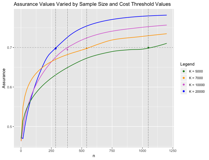
Figure 2: Assurance curves for each of the four different unit cost threshold cases $K$. Dotted vertical lines indicating when a presumed 0.70 assurance level is achieved according to O’Hagan and Stevens (from left to right): n = 285, n = 382, n = 541, and n = 1048.

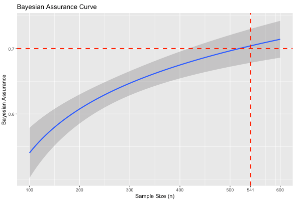
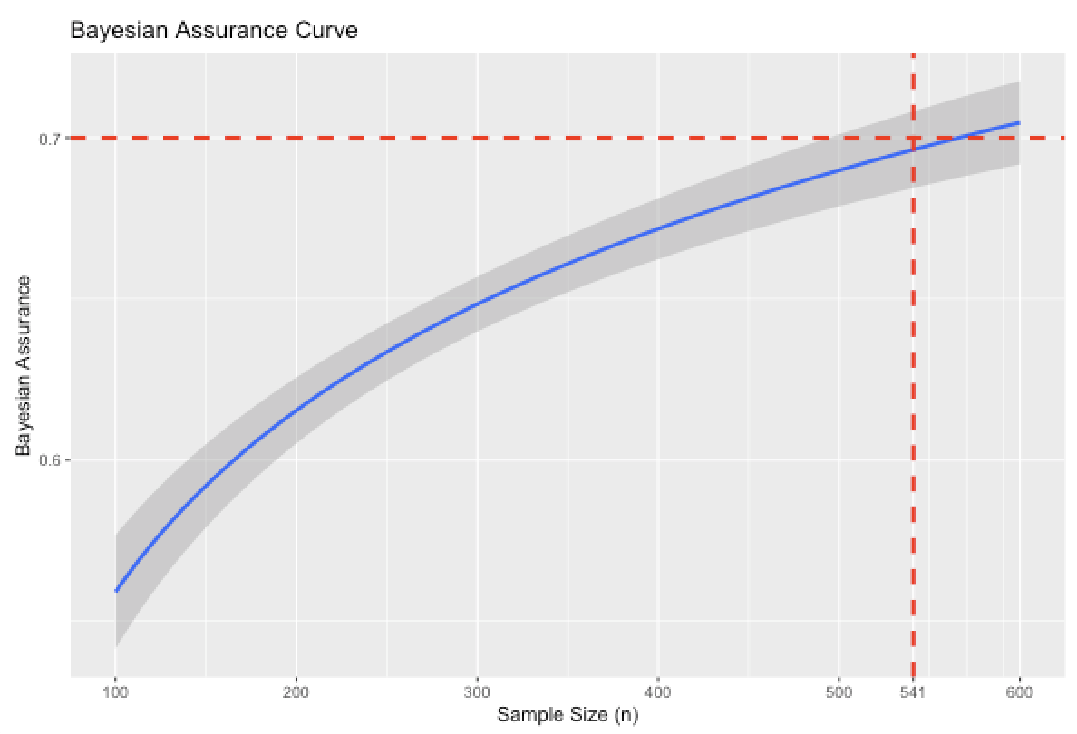
Figure 3: Resulting Bayesian assurance curves obtained from two separate simulation runs for the case with weak analysis priors and cost threshold value K = 7000.

Table 2: Selected subset of assurance values computed by algorithm for fixed variance case (note that many points were omitted here simply to make table more concise). Pairs highlighted in red correspond to the 4 points that were explicitly plotted in Figure 2.

K = 20000		K = 10000		K = 7000		K = 5000
n	Assurance	n	Assurance	n	Assurance	n	Assurance
1	0.473	1	0.463	1	0.463	1	0.470
185	0.655	282	0.673	440	0.687	500	0.667
205	0.669	332	0.693	490	0.694	750	0.689
235	0.687	382	0.695	541	0.698	875	0.699
285	0.697	482	0.716	640	0.712	1000	0.695
335	0.716	750	0.743	750	0.719	1048	0.700
1200	0.782	1200	0.758	1200	0.735	1200	0.710

We also provide a separate graphical display showcasing how the assurance behaves in separate runs to assess consistency in results. Figure 3 provides a side by side comparison of the assurance curves for the case, where the unit threshold cost is $K=7000$. The dotted red lines correspond to the 0.7 threshold and the effects of simulation errors can be seen through the slight differences in results between the two implementations. More specifically, the left image indicates that we achieve our 0.70 assurance level slightly before O’Hagan and Stevens, (2001) reported a sample size of $n=541$, whereas the right image shows that the assurance is achieved slightly after $n=541$. Such minor fluctuations are to be expected due to Monte Carlo errors in simulation.

3.2.2 Simulation Results in Unknown $\sigma^{2}$ Case

We now consider the setting where $\sigma^{2}$ is unknown. This extends the analysis in O’Hagan and Stevens, (2001) who treated the cost-effectiveness problem with fixed variances. Table 3 does not align as closely as the assurance results we had obtained from implementing the fixed $\sigma^{2}$ simulation in Section 3.2.1.

Referring to Table 3, we let $R$ be the number of outer loop iterations. The primary purpose of the outer loop is to randomly draw design stage variances $\sigma^{2(d)}$ from the $IG(a^{(d)},b^{(d)})$ distribution. Recall from Section 2.3.2 that $\sigma^{2(d)}$ is used for computing the variance of the marginal distribution from which we are drawing our sampled observations, $y\,|\,\sigma^{2(d)}$. The inner-loop iterations sample data using the marginal distribution of $\sigma^{2}$ from Equation (15). The number of iterations in the inner-loop is set to 750 for all cases. We notice that a majority of our trials report assurance values close to the 0.70 mark, particularly for the case in which we set the sample size to $n=1048$. The trial that exhibited the greatest deviation was for threshold cost $K=20000$ with corresponding sample size $n=285$, which returned an assurance of 0.58. This is most likely attributed to using a smaller sample size to gauge the effect size.

Outputs from Bayesian Assurance Algorithm
R	K =5000 n = 1048	K = 7000 n = 541	K = 10000 n = 382	K = 20000 n = 285
100	0.698	0.718	0.72	0.601
150	0.702	0.713	0.72	0.579

Table 3: Simulation results from the nonfixed Bayesian assurance algorithm with varying number of iterations in each of the four cost-effectiveness cases.

A visual depiction for this case can be seen in Figure 4.

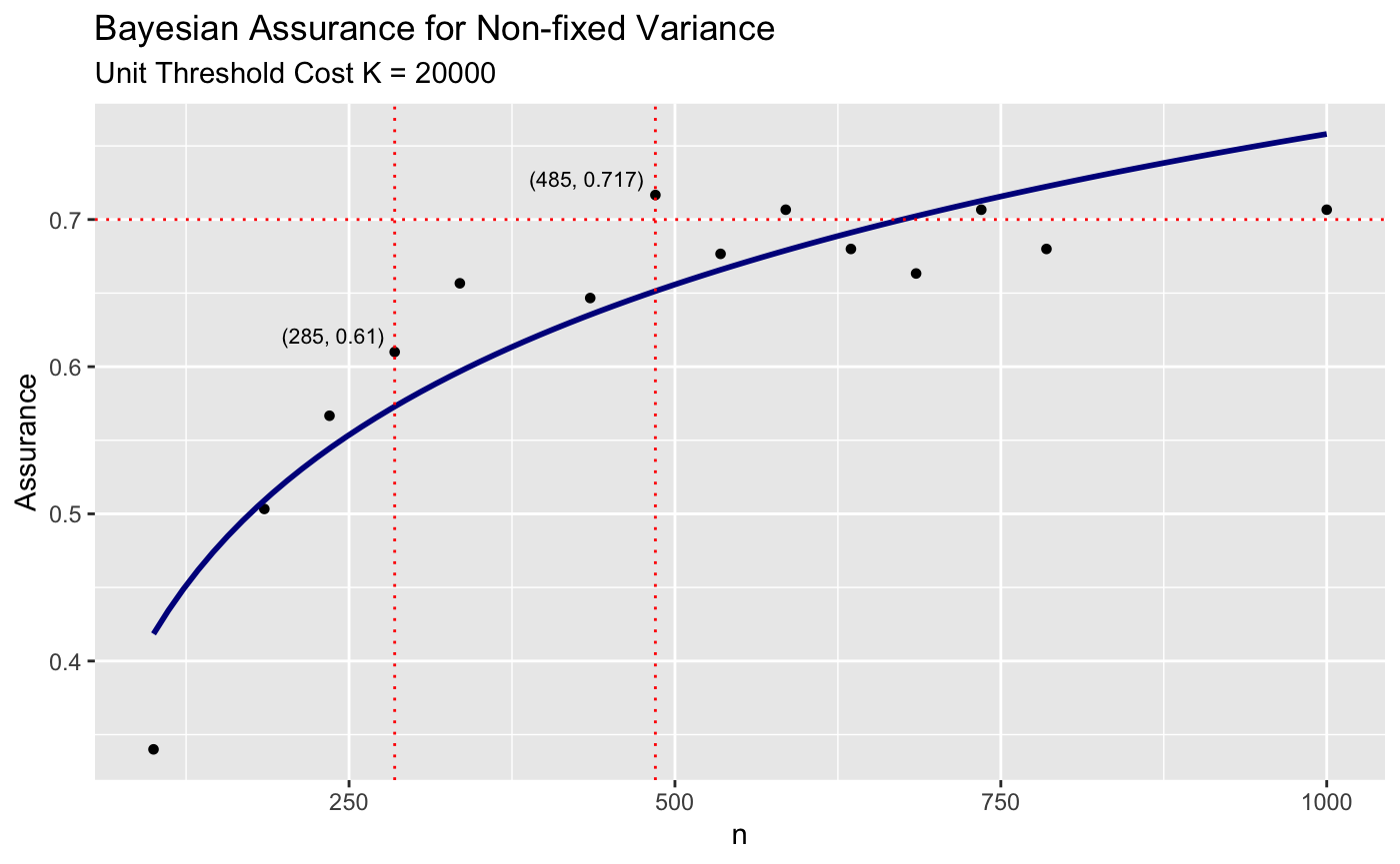
Figure 4: Assurance curve based on results of algorithm corresponding to unknown variance.

The dashed line on the left showcases the expected minimum sample size needed to achieve a 0.70 assurance whereas the dashed line on the right marks the point at which our algorithm actually achieves this desired threshold. The reality of the situation is that the problem setup gets changed quite a bit once we remove the assumption that $\sigma^{2}$ is known and fixed. If we look at the individual points marked on the plot, assurance values of 0.61 and 0.71 don’t appear too different. If we were to solely account for the fact that these Monte Carlo estimates are subject to error given that the estimates are based on means and variances that were compositely sampled rather than being taken in as fixed assignments, our algorithm performs remarkably well, but there are still points to be wary about.

The x-axis of the plot indicates that an assurance of 0.70 (red dotted line) can only be ensured once we recruit a sample size of at least $n=485$ per treatment group. This is substantially larger compared to the known $\sigma^{2}$ case, suggesting a need to recruit nearly twice as many participants as what was needed in Table 1. These results evince the pronounced impact of uncertainty in the design on the sample size needed to achieve a fixed level of Bayesian assurance.

3.3 Sample Size Determination with Precision-Based Conditions

We now consider a few alternate Bayesian approaches for sample size determination and demonstrate how these methods can be embedded within the two-stage Bayesian framework. We also identify special cases that overlap with the frequentist setting.

Adcock, (1997) constructs rules based on a fixed precision level $d$. In the frequentist setting, if $X_{i}\sim N(\theta,\sigma^{2})$ for $i=1,...,n$ observations and variance $\sigma^{2}$ is known, the precision can be calculated using $d=z_{1-\alpha/2}\frac{\sigma}{\sqrt{n}}$, where $z_{1-\alpha/2}$ is the critical value for the $100(1-\alpha/2)\%$ quartile of the standard normal distribution. Simple rearranging leads to following expression for sample size,

$$n=z_{1-\alpha/2}^{2}\frac{\sigma^{2}}{d^{2}}\;.$$ (18)

Given a random sample with mean $\bar{x}$, suppose the goal is to estimate population mean $\theta$. The analysis objective entails deciding whether or not the absolute difference between $\bar{x}$ and $\theta$ falls within a margin of error no greater than $d$. Given data $\bar{x}$ and a pre-specified confidence level $\alpha$, the assurance can be formally expressed as

$$\delta=P_{\bar{x}}\{\bar{x}:P(|\bar{x}-\theta|\leq d)\geq 1-\alpha\}\;.$$ (19)

To formulate the problem in the Bayesian setting, suppose $x_{1},\cdots,x_{n}$ is a random sample from $N(\theta,\sigma^{2})$ and the sample mean is distributed as $\bar{x}|\theta,\sigma^{2}\sim N(\theta,\sigma^{2}/n)$.

We assign $\theta\sim N(\theta_{0}^{(a)},\sigma^{2}/n_{a})$ as the analysis prior, where $n_{a}$ quantifies the amount of prior information we have for $\theta$. Adhering to the notation in previous sections, subscript $(a)$ denotes we are working within the analysis stage. Referring to Equation (19), the analysis stage objective is to observe if the condition, $|\bar{x}-\theta|\leq d$, is met. Recall that if the analysis objective holds to a specified probability level, then the corresponding sample size of the data being passed through the condition is sufficient in fulfilling the desired precision level for the study.

Additional steps can be taken to further expand out Equation (19). The posterior of $\theta$ can be obtained by taking the product of the prior and likelihood, giving us

$$N\Bigg{(}\bar{x}{\left|\theta,\frac{\sigma^{2}}{n}\right.}\Bigg{)}\times N\Bigg{(}\theta{\left|\theta_{0}^{(a)},\frac{\sigma^{2}}{n_{a}}\right.}\Bigg{)}=N\Bigg{(}\theta{\left|\lambda,\frac{\sigma^{2}}{n_{a}+n}\right.}\Bigg{)},$$ (20)

where $\lambda=\frac{n\bar{x}+n_{a}\theta_{0}^{(a)}}{n_{a}+n}$. From here we can further evaluate the condition using parameters from the posterior of $\theta$ to obtain a more explicit version of the analysis stage objective. Starting from $P(|\bar{x}-\theta|\leq d)=P(\bar{x}-d\leq\theta\leq\bar{x}+d)$, we can standardize all components of the inequality using the posterior parameter values of $\theta$, leading us to

$$P(|\bar{x}-\theta|\leq d)=P\left(\frac{\bar{x}-d-\lambda}{\sigma/\sqrt{n_{a}+n}}\leq\frac{\theta-\lambda}{\sigma/\sqrt{n_{a}+n}}\leq\frac{\bar{x}+d-\lambda}{\sigma/\sqrt{n_{a}+n}}\right)\\ =P\left(\frac{\bar{x}-d-\lambda}{\sigma/\sqrt{n_{a}+n}}\leq Z\leq\frac{\bar{x}+d-\lambda}{\sigma/\sqrt{n_{a}+n}}\right).$$

Simplifying the result gives us

$$\delta=\left\{\bar{x}:\Phi\left[\frac{\sqrt{n_{a}+n}}{\sigma}(\bar{x}+d-\lambda)\right]-\Phi\left[\frac{\sqrt{n_{a}+n}}{\sigma}(\bar{x}-d-\lambda)\right]\geq 1-\alpha\right\}.$$ (21)

Moving on to the design stage, we need to construct a protocol for sampling data that will be used to evaluate the analysis objective. This is achieved by first setting a separate design stage prior on $\theta$ such that $\theta\sim N(\theta_{0}^{(d)},\sigma^{2}/n_{d})$, where $n_{d}$ quantifies our degree of belief towards the population from which the sample will be drawn. Given that $\bar{x}|\theta,\sigma^{2}\sim N(\theta,\sigma^{2}/n)$, the marginal distribution of $\bar{x}$ can be computed using straightforward substitution based on $\bar{x}=\theta+\epsilon;$ $\epsilon\sim N(0,\sigma^{2}/n)$ and $\theta=\theta_{0}^{(d)}+\omega;$ $\quad\omega\sim N(0,\sigma^{2}/n_{d})$. Substitution $\theta$ into the expression for $\bar{x}$ gives us $\bar{x}=\theta_{0}^{(d)}+(\omega+\epsilon);$ $(\omega+\epsilon)\sim N\Big{(}0,\frac{\sigma^{2}(n_{d}+n)}{n_{d}n}\Big{)}=N(0,\sigma^{2}/p)$, where $1/p=1/n_{d}+1/n$. The marginal of $\bar{x}$ is therefore $N(\bar{x}|\theta_{0}^{(d)},\sigma^{2}/p)$, where we will be iteratively drawing our samples from to check if the sample means satisfy the condition derived in Equation (21). Algorithm 3 provides a skeleton of the code that was used to implement our simulations.

Algorithm 3 Bayesian assurance algorithm using Adcock’s condition for known variance in the univariate case

1:procedure bayes adcock($n$, $d$, $\theta_{0}^{(a)}$, $\theta_{0}^{(d)}$, $n_{a}$, $n_{d}$, $\sigma^{2}$, $\alpha$)

2:     count = $0$ $\triangleright$ keeps track of the iterations that satisfy the analysis obj

3:

4:     maxiter = $1000$ $\triangleright$ arbitrary number of iterations to loop thru

5:     for $i$ in range $1$ : maxiter do

6:         Design Stage Starts

7:         $\sigma^{2}_{d}\leftarrow\sigma^{2}\frac{n_{d}+n}{nn_{d}}$

8:         $\bar{x}\leftarrow$ single value generated from $N(\theta_{0}^{(d)},\sigma^{2}_{d})$

9:         Design Stage Ends

10:

11:         Analysis Stage Starts $\triangleright$ Computes components of the posterior distribution of parameter $\theta$:

12:         $\lambda\leftarrow\frac{n_{a}\theta_{0}^{(a)}+n\bar{x}}{n_{a}+n}$

13:         $\sigma^{2}_{a}\leftarrow\frac{\sigma^{2}}{n_{a}+n}$

14:         $\theta\leftarrow$ single value generated from $N(\lambda,\sigma^{2}_{a})$

15:

16:         $\phi_{1}\leftarrow\frac{\sqrt{n_{a}+n}}{\sigma}(\theta+d-\lambda)$

17:         $\phi_{2}\leftarrow\frac{\sqrt{n_{a}+n}}{\sigma}(\theta-d-\lambda)$

18:

19:         if $\Phi(\phi_{1})-\Phi(\phi_{2})\geq 1-\alpha$ then

20:              $Z_{i}\leftarrow 1$

21:         else

22:              if $\Phi(\phi_{1})-\Phi(\phi_{2})<1-\alpha$ then

23:                  $Z_{i}\leftarrow 0$

24:              end if

25:         end if

26:

27:         count $\leftarrow$ count + $Z_{i}$

28:         Analysis Stage Ends

29:     end for

30:

31:     assurance $\leftarrow$ count / maxiter

32:return assurance

33:

34:end procedure

3.3.1 Convergence to the Frequentist Setting

Unlike the cost-effectiveness application, the precision-based setting in Adcock, (1997) is not situated in a hypothesis testing framework. Hence, we cannot compute a set of corresponding power values that are directly comparable to our simulated assurance values. Nevertheless, an appropriate formulation of the analysis and design stage precision parameters, $n_{a}$ and $n_{d}$, can emulate this setting.

Referring to the derived expression for assurance in Equation (21), note that we are ultimately assessing whether the expression on the left hand side exceeds $1-\alpha$. Using the frequentist sample size formula given in Equation (18), we can work backwards from the sample size formula such that $1-\alpha$ is isolated on the right hand side of the inequality. We can then compare the expressions to compare the behaviors in relation to the probability of meeting the pre-specified condition. Starting from Equation (18), simple rearrangement reveals

$$n\geq z^{2}_{1-\alpha/2}\frac{\sigma^{2}}{d^{2}}\implies\frac{\sqrt{n}}{\sigma}d\geq z_{1-\alpha/2}\implies\Phi\Bigg{[}\frac{\sqrt{n}}{\sigma}d\Bigg{]}\geq 1-\alpha/2\implies 2\Phi\left[\frac{\sqrt{n}}{\sigma}d\right]-1\geq 1-\alpha.$$

If we refer back to Equation (21), it becomes clear that setting $n_{a}=0$ will simplify the expression down to the same expression we had previously obtained for the above frequentist scenario. Hence,

$$\delta=\left\{\bar{x}:\Phi\left[\frac{\sqrt{n_{a}+n}}{\sigma}(\bar{x}+d-\lambda)\right]-\Phi\left[\frac{\sqrt{n_{a}+n}}{\sigma}(\bar{x}-d-\lambda)\right]\geq 1-\alpha\right\}$$

$$\xRightarrow{n_{a}=0}\left\{\bar{x}:\Phi\left[\frac{\sqrt{n}}{\sigma}d\right]-\Phi\left[-\frac{\sqrt{n}}{\sigma}d\right]\geq 1-\alpha\right\}=\left\{\bar{x}:2\Phi\left[\frac{\sqrt{n}}{\sigma}d\right]-1\geq 1-\alpha\right\}.$$

In other words, if we let $\theta$ take on a weak analysis prior, we revert back to the frequentist setting in the analysis stage.

3.3.2 Simulation Results under Precision-Based Conditions

We test our algorithm using different fixed precision parameters $d$ with varying sample sizes $n$. The remaining fixed parameters including $\sigma^{2}$, $\theta_{0}^{(a)}$, and $\theta_{0}^{(d)}$ are randomly drawn from the uniform distribution Unif(0, 1) for simplicity sake. Figure 5 displays the results of the Bayesian-simulated points (marked in blue) in the case where weak analysis stage priors were assigned overlayed on top of the frequentist results (marked in red). Note that the Bayesian-simulated points denote the probability of observing that the posterior of $\theta$ differing from the sample mean $\bar{x}$ within a range of $\bar{x}\pm d$ exceeds $1-\alpha$.

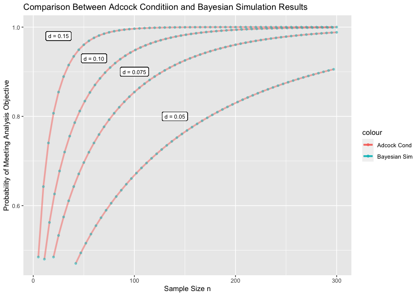
Figure 5: Overlay of simulated results and frequentist results given a weak analysis prior such that $n_{a}\rightarrow 0$.

From a general standpoint, these probabilities are obtained by iterating through multiple samples of size $n$ and observing the proportion of those samples that meet the analysis stage objective from Equation (21). As we have shown in the previous section, this becomes trivial in the case where weak analysis priors are assigned as we are left with a condition that is independent of $\bar{x}$. Hence, we are able to obtain the exact same probability values as those obtained from the frequentist formula. As shown in the plot, this can be seen across all sample sizes $n$ for all precision parameters $d$.

3.4 Sample Size Determination in a Beta-Binomial Setting

We revisit the hypothesis testing framework with proportions. Pham-Gia, (1997) outlines steps for determining exact sample sizes needed in estimating differences of two proportions in a Bayesian context. Let $p_{i},i=1,2$ denote two independent proportions. In the frequentist setting, suppose the hypothesis test to undergo evaluation is $H_{0}:p_{1}-p_{2}=0$ vs. $H_{a}:p_{1}-p_{2}\neq 0$. As described in Pham-Gia, (1997), one method of approach is to check whether or not $0$ is contained within the confidence interval bounds of the true difference in proportions given by $\displaystyle(\hat{p_{1}}-\hat{p_{2}})\pm z_{1-\alpha/2}(SE(\hat{p_{1}})^{2}+SE(\hat{p_{2}})^{2})^{1/2}$, where $z_{1-\alpha/2}$ denotes the critical region, and $SE(\hat{p_{i}})$ denotes the standard error of $p_{i}$ obtained by $SE(\hat{p_{i}})=\sqrt{\frac{\hat{p_{i}}(1-\hat{p_{i}})}{n_{i}}}$. An interval without $0$ contained within the bounds suggests there exists a significant difference between the two proportions.

The Beta distribution is often used to represent outcomes tied to a family of probabilities. The Bayesian setting uses posterior credible intervals as an analog to the frequentist confidence interval approach. As outlined in Pham-Gia, (1997), two individual priors are assigned to $p_{1}$ and $p_{2}$ such that $p_{i}\sim Beta(\alpha_{i},\beta_{i})$ for $i=1,2$. In the case of binomial sampling, $X$ is treated as a random variable taking on values $x=0,1,...,n$ to denote the number of favorable outcomes out of $n$ trials. The proportion of favorable outcomes is therefore $p=x/n$. Suppose a Beta prior is assigned to $p$ such that $p\sim Beta(\alpha,\beta)$. The prior mean and variance are respectively $\mu_{prior}=\frac{\alpha}{\alpha+\beta}$ and $\sigma^{2}_{prior}=\frac{\alpha\beta}{(\alpha+\beta)^{2}(\alpha+\beta+1)}$. Conveniently, given that $p$ is assigned a Beta prior, the posterior of $p$ also takes on a Beta distribution with mean and variance

$$\begin{split}\mu_{posterior}&=\frac{\alpha+x}{\alpha+\beta+n}\\ \sigma^{2}_{posterior}&=\frac{(\alpha+x)(\beta+n-x)}{(\alpha+\beta+n)^{2}(\alpha+\beta+n+1)}.\end{split}$$ (22)

Within the analysis stage, we assign two beta priors for $p_{1}$ and $p_{2}$ such that $p_{i}\sim Beta(\alpha_{i},\beta_{i}),i=1,2$. If we let $p_{d}=p_{1}-p_{2}$ and $p_{\text{post}}$ and $\text{var}(p)_{\text{post}}$ respectively denote the posterior mean and variance of $p_{d}$, it is straightforward to deduce that $p_{\text{post}}=\frac{\alpha_{1}+x_{1}}{\alpha_{1}+\beta_{1}+n_{1}}-\frac{\alpha_{2}+x_{2}}{\alpha_{2}+\beta_{2}+n_{2}}$ and $\text{var}(p)_{\text{post}}=\frac{(\alpha_{1}+x_{1})(\beta_{1}+n_{1}-x_{1})}{(\alpha_{1}+\beta_{1}+n_{1})^{2}(\alpha_{1}+\beta_{1}+n_{1}+1)}+\frac{(\alpha_{2}+x_{2})(\beta_{2}+n_{2}-x_{2})}{(\alpha_{2}+\beta_{2}+n_{2})^{2}(\alpha_{2}+\beta_{2}+n_{2}+1)}$ from Equation (22). Hence the resulting $100(1-\alpha)\%$ credible interval equates to $p_{\text{post}}\pm z_{1-\alpha/2}\sqrt{\text{var}(p)_{\text{post}}}$, which, similar to the frequentist setting, would be used to check whether $0$ is contained within the credible interval bands as part of our inference procedure. This translates to become our analysis objective, where we are interested in assessing if each iterated sample outputs a credible interval that does not contain $0$. We can denote this region of interest as $R(p)$ such that

$$R(p)=\left\{p:0\not\in\left(p_{\text{post}}-z_{1-\alpha/2}\sqrt{\text{var}(p)_{\text{post}}},\quad p_{\text{post}}+z_{1-\alpha/2}\sqrt{\text{var}(p)_{\text{post}}}\right)\right\}.$$ (23)

It follows that the corresponding assurance for assessing a significant difference in proportions can be computed as

$$\delta=P\left\{p_{d}:0\not\in\left(p_{\text{post}}-z_{1-\alpha/2}\sqrt{\text{var}(p)_{\text{post}}},\quad p_{\text{post}}+z_{1-\alpha/2}\sqrt{\text{var}(p)_{\text{post}}}\right)\geq 1-\alpha\right\}.$$

Moving on to the design stage, note that the simulated data in Beta-Binomial setting pertains to the frequency of positive outcomes, $x_{1}$ and $x_{2}$, observed among the two samples. These frequency counts are observed from samples of size $n_{1}$ and $n_{2}$ based on given probabilities, $p_{1}$ and $p_{2}$, that are passed in the analysis stage. Once $p_{1}$ and $p_{2}$ are assigned, $x_{1}$ and $x_{2}$ values are randomly generated from their corresponding binomial distributions, where $x_{i}\sim Bin(n_{i},p_{i}),i=1,2$. The posterior credible intervals are subsequently computed to undergo assessment in the analysis stage. These steps are repeated iteratively starting from the generation of $x_{1}$ and $x_{2}$ values. The proportion of iterations with results that fall within the region of interest expressed in Equation (23) equates to the assurance. Algorithm 4 provides a skeleton of the code used to implement our simulations.

Algorithm 4 Bayesian assurance algorithm for difference in two independent proportions under Pham-Gia’s credible interval condition

1:procedure bayes pham-gia($n_{1}$, $n_{2}$, $p_{1}=\text{NULL}$, $p_{2}=\text{NULL}$, $\alpha_{1}$, $\alpha_{2}$, $\beta_{1}$, $\beta_{2}$, $\alpha$)

2:     if $\psi=1$ then

3:         $p_{1}\leftarrow$ single value generated from $\text{Unif}[p_{1},p_{1}]$

4:         $p_{2}\leftarrow$ single value generated from $\text{Unif}[p_{2},p_{2}]$

5:     else if $\psi=0$ then

6:         $p_{1}\leftarrow$ $\text{Beta}(\alpha_{1},\beta_{1})$

7:         $p_{2}\leftarrow$ $\text{Beta}(\alpha_{2},\beta_{2})$

8:     end if

9:

10:     count = $0$ $\triangleright$ keeps track of the iterations that satisfy the analysis obj

11:     maxiter = $1000$ $\triangleright$ arbitrary number of iterations to loop thru

12:

13:     for $i$ in range $1$ : maxiter do

14:         Design Stage Starts

15:         $x_{1}\leftarrow$ single value generated from $Bin(n_{1},p_{1})$

16:         $x_{2}\leftarrow$ single value generated from $Bin(n_{2},p_{2})$

17:         Design Stage Ends

18:

19:         Analysis Stage Starts

20:         $p_{\text{post}}=\frac{\alpha_{1}+x_{1}}{\alpha_{1}+\beta_{1}+n_{1}}-\frac{\alpha_{2}+x_{2}}{\alpha_{2}+\beta_{2}+n_{2}}$ $\triangleright$ Computes posterior parameters of $p=p_{1}-p_{2}$

21:         $\text{var}(p)_{\text{post}}=\frac{(\alpha_{1}+x_{1})(\beta_{1}+n_{1}-x_{1})}{(\alpha_{1}+\beta_{1}+n_{1})^{2}(\alpha_{1}+\beta_{1}+n_{1}+1)}+\frac{(\alpha_{2}+x_{2})(\beta_{2}+n_{2}-x_{2})}{(\alpha_{2}+\beta_{2}+n_{2})^{2}(\alpha_{2}+\beta_{2}+n_{2}+1)}$

22:

23:         lb = $p_{\text{post}}-z_{1-\alpha/2}\sqrt{var(p)_{\text{post}}}$ $\triangleright$ Computes upper and lower bounds

24:         ub = $p_{\text{post}}+z_{1-\alpha/2}\sqrt{var(p)_{\text{post}}}$

25:

26:         if $0<$ lb or $0>$ ub then

27:              count $\leftarrow$ count + $1$

28:         end if

29:         Analysis Stage Ends

30:     end for

31:

32:     assurance $\leftarrow$ count / maxiter

33:return assurance

34:

35:end procedure

3.4.1 Relation to Frequentist Setting

It is worth pointing out that there are no precision parameters to quantify the amount of information we have on the priors being assigned. Directly showcasing parallel behaviors between Bayesian and frequentist settings involve knowing the probabilities beforehand and passing them in as arguments into the simulation. Specifically, if $p_{1}$ and $p_{2}$ are known beforehand, we can express these “exact” priors as Uniform distributions such that $p_{i}\sim\text{U}[p_{i},p_{i}]$. We can then express the overall analysis stage prior as a probability mass function:

$$p_{i}=\psi\text{Unif}[p_{i},p_{i}]+(1-\psi)\text{Beta}(\alpha_{i},\beta_{i}),\quad i=1,2,$$

where $\psi$ denotes the binary indicator variable for knowing exact values of $p_{i}$ beforehand. If $\psi=1$, we are drawing from the uniform distribution under the assumption of exact priors. Otherwise, $\psi=0$ and we draw from the beta distribution to evaluate the analysis stage objective.

There is also an additional route we can use to showcase overlapping behaviors between the Bayesian and frequentist paradigms. Recall the sample size formula for assessing differences in proportions in the frequentist setting,

$$n=\frac{(z_{1-\alpha/2}+z_{\beta})^{2}(p_{1}(1-p_{1})+p_{2}(1-p_{2}))}{(p_{1}-p_{2})^{2}},$$

where $n=n_{1}=n_{2}$. Simple rearragements and noting that $-(z_{1-\alpha/2}+z_{\beta})=z_{1-\beta}-z_{1-\alpha/2}$ lead us to obtain

$$\frac{\sqrt{n}(p_{1}-p_{2})}{\sqrt{p_{1}(1-p_{1})+p_{2}(1-p_{2})}}+z_{1-\alpha/2}=z_{1-\beta}\implies\text{Power}=1-\beta=\\ \Phi\left(\frac{\sqrt{n}(p_{1}-p_{2})}{\sqrt{p_{1}(1-p_{1})+p_{2}(1-p_{2})}}+z_{1-\alpha/2}\right).$$

In an ideal situation, we could determine suitable parameters for $\alpha_{i}$, $\beta_{i}$, $i=1,2$ to use as our Beta priors that would enable demonstration of convergence towards the frequentist setting. However, a key relationship to recognize is that the Beta distribution is a conjugate prior of the Binomial distribution. There is a subtle advantage offered given that the Bayesian credible interval bands are based upon posterior parameters of the Beta distribution and the frequentist confidence interval bounds are based upon the Binomial distribution. Because of the conjugate relationship held by the Beta and Binomial distributions, we are essentially assigning priors to parameters in the Bayesian setting that the Binomial density in the frequentist setting is conditioned upon. Using the fact that the normal distribution can be used to approximate binomial distributions for large sample sizes given that the Beta distribution is approximately normal when its parameters $\alpha$ and $\beta$ are set to be equal and large. We manually choose such values and apply them to our simulation study.

3.4.2 Simulation Results

Figure 6 displays the assurance curves overlayed on top of the frequentist power curves. As mentioned in the previous section, we manually set the parameters of the beta priors to be equal as doing so results in approximately normal behavior. The horizontal line at the top of the graph corresponds to flat priors for the beta distribution known as Haldane’s priors, in which the $\alpha$ and $\beta$ parameters are all set to 0.5. Although the points do not align perfectly with the frequentist curves as we rely on an approximate relationship rather than identifying prior assignments that allow direct ties to the frequentist case, our model still performs fairly well as the points and curves are still relatively close to one another.

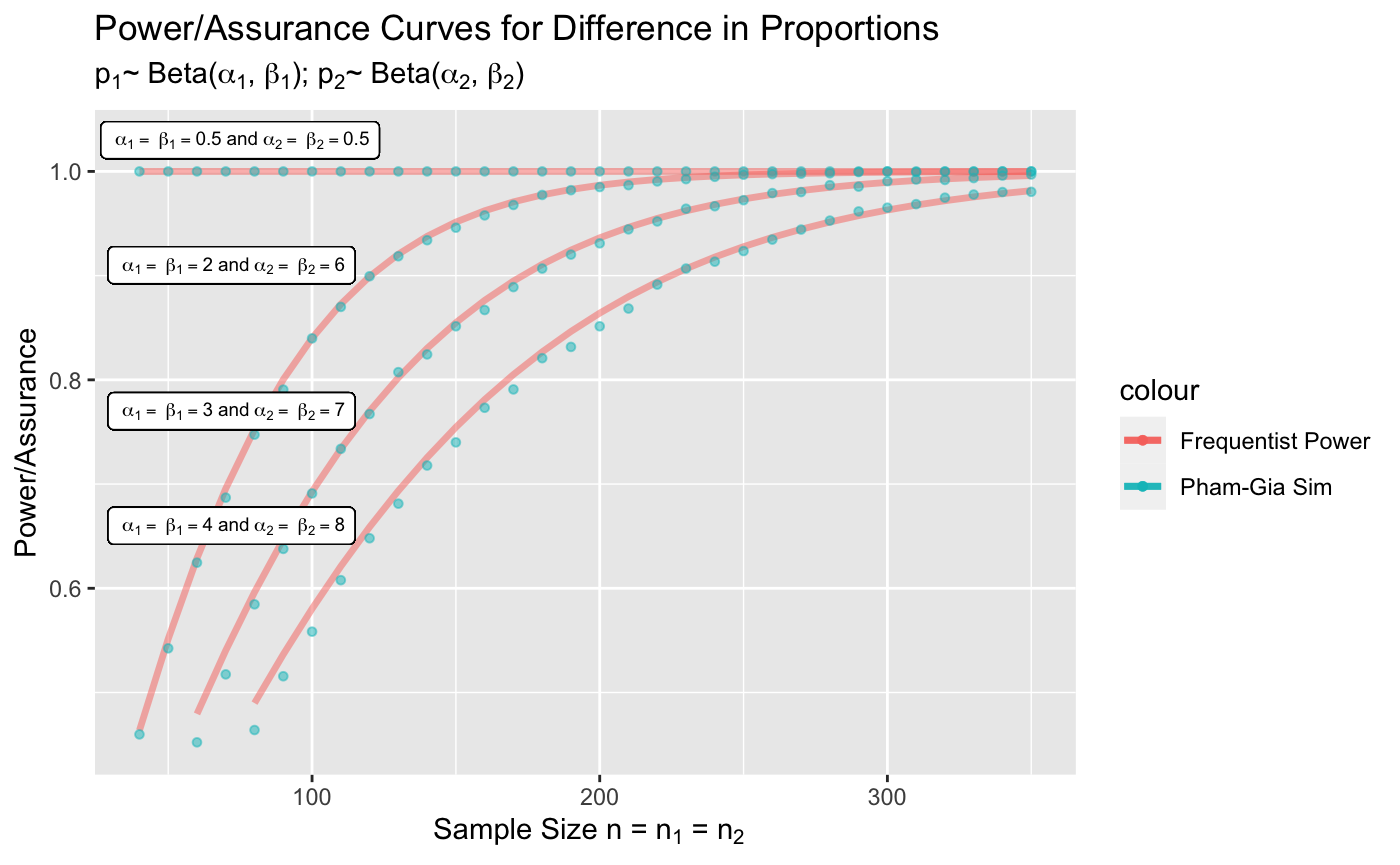
Figure 6: Overlay of simulated assurance results using posterior credible intervals and frequentist power results based on regular confidence intervals.

4 Discussion

This paper has attempted to present a simulation-based Bayesian design framework for sample size calculations using assurance for deciding in favor of a hypothesis (analysis objective). It is convenient to describe this framework in two stages: (i) the design stage generates data from a population modeled using design priors; and (ii) the analysis stage performs customary Bayesian inference using analysis priors. The frequentist setting emerges as a a special case of the Bayesian framework with highly informative design priors and completely uninformative analysis priors.

Our framework can be adapted and applied to a variety of clinical trial settings. Future directions of research and development can entail incorporating more complex analysis objectives into our framework. For example, the investigation of design and analysis priors in the use of Go/No Go settings (Pulkstenis et al.,, 2017), which refers to the point in time at which enough evidence is present to justify advancement to Phase 3 trials, will be relevant. Whether the method of choice involves looking at lengths of posterior credible intervals (Joseph et al.,, 1997) or determining cutoffs that minimize the weighted sum of Bayesian average errors (Reyes and Ghosh,, 2013), such conditions are all capable of being integrated as part of our analysis stage objective within our two-stage paradigm.

References

- Adcock, (1997) Adcock, C. (1997). Sample size determination: A review. The Statistician, 46(2).
- Berger, (1985) Berger, J. O. (1985). Statistical Decision Theory and Bayesian Analysis. Springer New York, New York, NY.
- Berry, (2006) Berry, D. A. (2006). Bayesian clinical trials. Nature Reviews Drug Discovery, 5(1).
- Berry et al., (2010) Berry, S. M., Carlin, B. P., Lee, J. J., and Müller, P. (2010). Bayesian Adaptive Methods for Clinical Trials. Chapman & Hall/CRC Biostatistics Series, United Kingdom.
- Cohen, (1988) Cohen, J. (1988). Statistical Power Analysis for the Behavioral Sciences (2nd ed.). Lawrence Erlbaum Associates, Hillsdale, NJ.
- Desu and Raghavarao, (1990) Desu, M. and Raghavarao, D. (1990). Sample Size Methodology. Elsevier, Massachusetts.
- Gelfand and Wang, (2002) Gelfand, A. E. and Wang, F. (2002). A simulation based approach to bayesian sample size determination for performance under a given model and for separating models. Statistical Science, 17(2).
- Gelman et al., (2013) Gelman, A., Carlin, J. B., and Stern, H. S. (2013). Bayesian Data Analysis (3rd ed.). Chapman and Hall/CRC, United Kingdom.
- Ibrahim et al., (2012) Ibrahim, J. G., Chen, M.-H., Xia, A., and Liu, T. (2012). Bayesian meta-experimental design: Evaluating cardiovascular risk in new antidiabetic therapies to treat type 2 diabetes. Biometrics, 68(2).
- Joseph et al., (1997) Joseph, L., Berger, R. D., and Belisle, P. (1997). Bayesian and mixed bayesian/likelihood criteria for sample size determination. Statistics in Medicine, 16(7).
- Kraemer and Thiemann, (1987) Kraemer, H. C. and Thiemann, S. (1987). How Many Subjects? Statistical Power Analysis in Research. Sage Publications, Newbury Park.
- Lee and Chu, (2012) Lee, J. and Chu, C. T. (2012). Bayesian clinical trials in action. Statistics in Medicine, 31(25).
- Lee and Zelen, (2000) Lee, S. J. and Zelen, M. (2000). Clinical trials and sample size considerations: Another perspective. Statistical Science, 15(2).
- Lindley, (1997) Lindley, D. V. (1997). The choice of sample size. The Statistician, 46(2).
- Liu and Liang, (1997) Liu, G. and Liang, K. Y. (1997). Sample size calculations for studies with correlated observations. Biometrics, 53(3).
- Muller et al., (1992) Muller, K. E., Lavange, L. M., Ramey, S. L., and Ramey, C. T. (1992). Power calculations for general linear multivariate models including repeated measures applications. Journal of the American Statistical Association, 87(420).
- Müller and Parmigiani, (1995) Müller, P. and Parmigiani, G. (1995). Optimal design via curve fitting of monte carlo experiments. Journal of the American Statistical Association, 90(432).