Graph Neural Networks Accelerated Molecular Dynamics

Abstract

Molecular Dynamics (MD) simulation is a powerful tool for understanding the dynamics and structure of matter. Since the resolution of MD is atomic-scale, achieving long time-scale simulations with femtosecond integration is very expensive. In each MD step, numerous iterative computations are performed to calculate energy based on different types of interaction and their corresponding spatial gradients. These repetitive computations can be learned and surrogated by a deep learning model like a Graph Neural Network (GNN). In this work, we developed a GNN Accelerated Molecular Dynamics (GAMD) model that directly predicts forces given the state of the system (atom positions, atom types), bypassing the evaluation of potential energy. By training the GNN on a variety of data sources (simulation data derived from classical MD and density functional theory), we show that GAMD can predict the dynamics of two typical molecular systems, Lennard-Jones system and Water system, in the NVT ensemble with velocities regulated by a thermostat. We further show that GAMD’s learning and inference are agnostic to the scale, where it can scale to much larger systems at test time. We also perform a comprehensive benchmark test comparing our implementation of GAMD to production-level MD softwares, showing GAMD’s competitive performance on the large-scale simulation.

MechE]Department of Mechanical Engineering, Carnegie Mellon University, Pittsburgh PA, USA MechE]Department of Mechanical Engineering, Carnegie Mellon University, Pittsburgh PA, USA MechE]Department of Mechanical Engineering, Carnegie Mellon University, Pittsburgh PA, USA MechE]Department of Mechanical Engineering, Carnegie Mellon University, Pittsburgh PA, USA [ML]Machine Learning Department, Carnegie Mellon University, Pittsburgh PA, USA [Chem]Department of Chemical Engineering, Carnegie Mellon University, Pittsburgh PA, USA

1 Introduction

Molecular Dynamics (MD) has been extensively used in a wide range of applications in material science, physical chemistry, and biophysics during the last decades ^{1, 2}. MD simulations can provide the understanding and precise predictions of many intricate systems. MD simulations rely on the knowledge of forces acting on every particle in the system and solving equations of motion to generate the trajectories of atoms in an iterative manner. Ab initio approaches like density functional theory (DFT) ³ are more accurate methods that consider the electronic structure of atoms. However, they are prohibitively time-expensive, especially for large many-body systems ⁴. Alternatively, forces can be calculated from empirical interatomic potentials for different environments bypassing the electronic structures in the system, resulting in faster simulations than ab initio methods⁵. Nevertheless, MD simulations have limitations including their long computational times ⁶, as well as the accuracy and generalizability of the empirical potentials ^{4, 5}. We will expand upon these two aspects in the following paragraphs.

The first major limitation of Molecular Dynamics is its computational intensity. Ensuring the stability of MD simulations with atomic-scale resolution requires integration time steps in the order of femtoseconds. This imposes a significant time constraint for many biochemical and macromolecular systems which have much longer time scales of dynamics (nano- or micro-seconds), such as simulating large scale systems like viruses for realistic time scales ^{1, 6, 7}. Achieving these long time-scale simulations is compute-intensive, or even impossible in some cases, despite using state-of-the-art computational hardware, such as GPUs, and acceleration techniques.

Each iteration of MD simulations requires a huge amount of computations including the calculation of forces acting on each particle summed up from various bonded or non-bonded potentials in the system ⁵. Depending on the type and the scale of the simulations, they contain many repetitive computations especially in calculating forces for each atom as the negative gradient of the empirical potentials ^{8, 9}. Avoiding these time-consuming and iterative steps provides an opportunity to conduct more time-efficient MD simulations ^{10, 11, 9}. Another promising approach to reduce the amount of computation in complex systems has been through the coarse-grained force fields ¹². However, while some thermodynamic consistency can be preserved by coarse-grained networks, there is still considerable information loss on structural details and properties of the systems ^{13, 14}.

The second major limitation of classical MD simulations stems from the limitation of accuracy in calculations and approximations required to describe complex interatomic potentials between particles. There are a wide variety of interactions depending on the types of particles (bonded or non-bonded interactions), and the system composition. Finding the appropriate functional forms that satisfy the precision requirement is a challenging task ^{5, 15}. Recently, machine learning (ML) has been viewed as a promising candidate for learning force fields ^{16, 17, 18, 19, 20, 21, 22, 23, 24, 25, 26, 27}.

In the last decade, advances in machine learning have enabled learning the dynamics of many complex physics-based systems from training data. Currently, there are active avenues of research with aim to learn models which simulate complex systems governed by well-known, partially-known, or even unknown underlying physics ^{28, 29, 30}. The learnt model can accurately approximate the true physical model, and in some cases, accelerate the simulation, prediction, and control of the systems by surrogating the full physics model ⁹. In addition to the gain in time efficiency, proposed models have to perform well in terms of both accuracy (within the training data distribution) and generalization (beyond the data what the model is trained on). The capabilities of ML, especially neural networks, in learning arbitrary functional forms have made them a suitable choice for the task of learning interatomic potentials in MD ^{31, 22, 17, 16, 32}.

The initial approaches to use machine learning to learn force fields have leveraged feature engineering methods, by finding tailored descriptors that capture the characteristics of the local environment of atoms in the system ^{31, 20, 33, 34, 35, 36}. Atom-centered symmetry functions (ACSFs), used in Behler-Parrinello Neural Networks (BPNN) ^{37, 38, 39}, is one of the first examples of using such descriptors for translation- and rotation-invariant energy conservation. Recent advancements of deep neural networks, with automatic feature extraction capabilities, have made it possible to learn the atomic representations directly from the raw atomic coordinates and low-level atomic features, providing an alternative to the manually tailored atomic fingerprints ^{40, 41, 42, 43, 44, 45, 46}. Due to the unstructured position of particles and their limited interactions in an MD system, graph neural networks (GNNs) can be a suitable choice to approach this task ^{41, 11}.

Graph Neural Networks (GNNs), with convolution layers that are specialized for unstructured data, have recently been used to learn various physics-based models and to accelerate them ^{47, 48, 49, 50, 51, 52}. In molecular systems they have shown a performance boost as well as an end-to-end learning opportunity that bypasses the need for manual feature representations by learning the properties automatically from the atomic observations ^{40, 53, 54, 55}. GNNs encode information about particles (their properties and the neighbor interactions) in the nodes and edges of a defined graph. The neighbor interactions can be described in the general form of message passing neural networks (MPNNs) ⁵⁶ where information is passed between neighbor atoms, i.e. nodes, in the graph.

A distinction between ML models for learning forces in MD simulations can be classified as energy-centric and force-centric models ^{9, 11}. Energy-centric models aim to learn the potential energy surface (PES) and obtain forces by calculating derivatives of the PES ⁸. The majority of the currently proposed ML models belong to this group and directly conserve the system’s energy due to their architecture and loss function design ^{41, 43}. Gradient-Domain Machine Learning (GDML) and symmetrized GDML (sGDML) ^{8, 21} conserve energy by learning explicit gradient function mapping of energy and interatomic forces. Another energy-centric model, SchNet ⁴⁴ employs continuous convolution filters to learn features on graph networks for smooth energy predictions. DimeNet ^{57, 58} is another more complex energy-centric model that, though slower than SchNet, shows better generalization to different molecules and configurations by having angular information in the feature updates. Several deep learning frameworks have been built based on differentiable physics to employ classical MD and machine learning potentials learned by these energy-centric models ^{59, 60, 61, 62}.

In the force-centric group of models, forces are predicted directly by using networks where the forces predicted by the model, which are then compared against the ground truth forces. In other words, the network’s outputs are per-node, i.e. per-atom, forces ^{9, 10, 11}. While these models do not possess any strict energy conservation mechanism, they have promising features. One challenge with the prediction of forces from PES has been the amplification of noise and error in taking derivatives of energy. This issue has been addressed to an extent by considering terms of both force and energy in the loss function ^{63, 44, 8}. However, using a force-only training model can result in better force prediction accuracy ⁶⁴. The main benefit of using force-centric models is the computational efficiency brought about by avoiding additional calculations required for computing forces in the energy-centric models. These calculations include taking derivatives from the accumulation of several types of potential energies ^{9, 11}.

Force-centric models have been applied in several applications to infer the forces in fluids ²⁸, glassy systems, and solid-state MD simulations ^{29, 10, 11}, as well as large-scale quantum property calculations ⁹. Bypassing the calculations required for taking derivatives of PES has provided gains in computational efficiency for neural network force field (NNFF) ¹⁰ and Graph NNFF (GNNFF) ¹¹ models. By using the DFT-calculated forces as ground truth, GNNFF can learn atomistic level dynamics of solid-state material systems. A force-centric model, ForceNet ⁹ uses Graph Network-based simulators (GNS) framework to predict forces by using a massive physics-based augmented dataset rather than applying any architectural constraints. These models show faster and accurate predictions of quantum properties and forces in comparison to energy-centric models like SchNet ⁴⁴.

The energy- and force-centric models have been two lines of research to approach the aforementioned limitations of MD. On one hand, exploiting the power of deep neural networks and differentiable programming to automatically learn representations from the basic atomic features and coordinates has led to more generalizable potential models ^{26, 59, 60}. On the other hand, force-centric models avoid the computational bottleneck of taking derivatives and provide faster force predictions ^{9, 11}. In this work, we combine these two aspects in a Graph Accelerated Molecular Dynamics (GAMD) framework, where we leverage GNNs to learn atomic representations and directly predict per-atom forces from these learned features. We show that by careful training of a rotation-covariant graph model, we can bypass the physics-based neighbor selection and energy calculation steps of traditional MD simulations. In other words, GAMD avoids the computational bottleneck of calculating spatial derivatives from PES in long time scale molecular dynamics. Since GAMD does not derive the forces from PES, it does not conserve potential energy, but it can be used to run the simulation in an NVT ensemble where velocities are regulated by a thermostat of proper intensity. Our work is closely related to prior works on developing force-centric models - NNFF¹⁰, GNNFF ¹¹ and ForceNet ⁹. Similar to GNNFF and ForceNet, we use GNN as the backbone to build a molecular force model, however, with different architectures (message passing function and input edge features). Moreover, in this work we investigate the applicability and scalability of using a force-centric model to accelerate the dynamics on the large-scale molecular system such as water system ^{65, 66, 67} and conduct a detailed evaluation of the computational time efficiency.

2 Methods

2.1 Molecular Representation

A molecular system at a certain state can be described as: $\mathbf{X}:(\mathbf{q}_{1},\mathbf{q}_{2},\dots,\mathbf{q}_{n})$, where $\mathbf{q}_{i},\forall i\in\{1,2,\dots,n\}$ denotes the Cartesian coordinates of each atom in the system. Through the network, we represent atoms as nodes in a GNN and interactions between atoms as edges. Concretely, the node input feature is a one-hot vector $\mathbf{p}_{i}$, which specifies the atom type. The edge input feature is a vector derived by concatenating inter-atomic distance vector $\mathbf{q}_{ij}$ and a one-hot vector $\mathbf{b}_{ij}$ which indicates the edge type between two atoms (i.e. whether two atoms are bonded in the same molecule). The inter-atomic distance vector is defined by concatenating the directional vector and the norm of relative position: $\mathbf{q}_{ij}=(\frac{\mathbf{q}_{i}-\mathbf{q}_{j}}{||\mathbf{q}_{i}-\mathbf{q}_{j}||_{2}},||\mathbf{q}_{i}-\mathbf{q}_{j}||_{2})$. With the introduction of directional vector, the edge is directed, therefore $\mathbf{e}_{ij}\neq\mathbf{e}_{ji}$. In addition, this makes the network rotational covariant as directional vector varies when the system rotates.

To further leverage the expressiveness of neural networks, we lift node input features $\mathbf{p}_{i}$ and edge input features $(\mathbf{q}_{ij},\mathbf{b}_{ij})$ into high-dimensional vector embedding $\mathbf{v}^{(0)}_{i},\mathbf{e}^{(0)}_{ij}\in\mathbb{R}^{d}$ (with $d$ being the dimension of latent space) via learnable encoders $\epsilon^{V}$ and $\epsilon^{E}$ (Figure 1, Feature Encoding), which are built upon multi-layer perceptrons (MLPs).

$$\begin{split}\mathbf{v}^{(0)}_{i}&=\epsilon^{V}(\mathbf{p}_{i})\\ \mathbf{e}^{(0)}_{ij}&=\epsilon^{E}(\mathbf{q}_{ij},\mathbf{b}_{ij})\end{split}$$ (1)

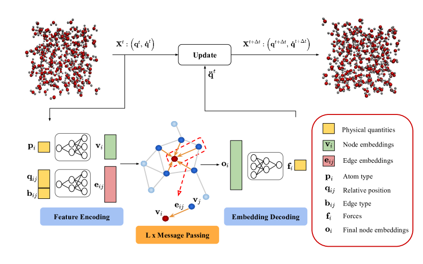
Figure 1: Overview of GAMD schematic. GAMD uses graph neural network (GNN) to predict the forces of atoms $\mathbf{f}_{i}$ in the molecular system $\forall i\in\{1,2,\dots,n\}$ given properties of atoms $\mathbf{p}_{i}$ (i.e. type of atoms), positions of atoms $\mathbf{q}_{i}$, and edge type between each pair of atoms $\mathbf{b}_{ij}$ (bond information). The features are first encoded using multi-layer perceptron (MLPs) and then inferred using an atom-wise message passing scheme. At last, an MLP decoder predicts forces from the node embeddings. Based on the predicted forces, GAMD forwards the dynamics of the system by imposing acceleration $\mathbf{\ddot{q}}$ on each atom.

2.2 Atom-wise Message Passing

The inference and prediction of molecular information utilizes a recurring atom-wise message passing block (Figure 1, Message Passing). Inside each block, the center atom $i$ first collects messages from all the neighbor atoms $\forall j\in\mathcal{N}(i)$. The message $\mathbf{m}^{(l)}_{j\rightarrow i}$ is conditioned on the edge embedding $\mathbf{e}^{(l-1)}_{ij}$ which carries the inter-atomic directional information and interaction type between two particles, along with node features from source atom $\mathbf{v}^{(l-1)}_{j}$ and target atom $\mathbf{v}^{(l-1)}_{i}$:

$$\mathbf{m}^{(l)}_{j\rightarrow i}=\Phi^{(l)}\left(\mathbf{v}^{(l-1)}_{j},\mathbf{e}^{(l-1)}_{ij},\mathbf{v}^{(l-1)}_{i}\right)\odot\mathbf{v}^{(l-1)}_{j},\forall j\in\mathcal{N}(i)$$ (2)

Where $\Phi^{(l)}:\mathbb{R}^{d}\times\mathbb{R}^{d}\times\mathbb{R}^{d}\rightarrow\mathbb{R}^{d}$ is the learnable message function at the $l-th$ block, and $\odot$ denotes element-wise multiplication. The message passing mechanism adopted here can also be viewed as an extension of continuous convolution proposed in SchNet ⁴⁴, with a learnable filter conditioned not only on inter-atomic distances but also interaction types between atoms, and atom properties of source and target atoms.

After all messages from neighbor atoms are collected, they are aggregated together and used to update the node embeddings.

$$\mathbf{M}^{(l)}_{i}=\sum_{\forall j\in\mathcal{N}(i)}\mathbf{m}^{(l)}_{j\rightarrow i}$$ (3)

$$\mathbf{\hat{v}}^{(l)}_{i}=\Theta^{(l)}\left(\mathbf{v}^{(l-1)}_{i},\mathbf{M}^{(l)}_{i}\right)$$ (4)

Where $\Theta^{(l)}:\mathbb{R}^{d}\times\mathbb{R}^{d}\rightarrow\mathbb{R}^{d}$ is the learnable node update function at the $l-th$ block. We apply layer-normalization ⁶⁸ to the node embedding before inputting into each message passing layer and use residual connection ⁶⁹ at every message passing layer.

We implement the message function $\Phi$, and the node update function $\Theta$ as MLPs. Notice that, throughout the network, only the node embeddings are updated recursively, the edge embeddings at per-layer are derived via a learnable non-linear transformation $\mathbf{A}(\cdot)$ (which is also implemented as MLP) from the initial encoded edge embeddings: $e^{(l)}_{ij}=\mathbf{A}^{(l)}(e^{(0)}_{ij}$). In general, we find that disabling edge embedding’s recursive update will not result in performance degradation, yet it can reduce the overall computational cost (ablation study on the influence of recursive edge embedding update can be found in Section 2 in the Supplementary Information).

2.3 Graph Neural Force Predictor

The learnable decoder $\gamma^{V}:\mathbb{R}^{d}\rightarrow\mathbb{R}^{3}$ decodes high-dimensional node embeddings $\mathbf{o}$ ($\mathbf{o}_{i}=\mathbf{v}_{i}^{(l)},\forall i\in{1,2,\dots,N}$) at the final layer into the Cartesian forces $\mathbf{f}$ (Figure 1, Embedding Decoding). The predicted forces are then used to update the acceleration $\mathbf{\ddot{q}}$ of each atom. The GNN-based force predictor can be flexibly integrated into any numerical integrator that has a force-based scheme. For instance, a single step in the Velocity-Verlet with GNN-based force predictor $\mathbf{\mathcal{F}(\cdot)}$ can be written as:

$$\mathbf{\dot{q}}_{t+\Delta t/2} =\mathbf{\dot{q}}_{t}+\mathbf{\ddot{q}}_{t}\Delta t/2$$ (5)

$$\mathbf{q}_{t+\Delta t} =\mathbf{q}_{t}+\mathbf{\dot{q}}_{t+\Delta t/2}\>\Delta t$$ (6)

$$\mathbf{\ddot{q}}_{t+\Delta t} =\mathbf{\mathcal{F}}\left(\mathbf{p},\mathbf{b},\mathbf{q}_{t+\Delta t}\right)/\mathbf{m}$$ (7)

$$\mathbf{\dot{q}}_{t+\Delta t} =\mathbf{\dot{q}}_{t+\Delta t/2}+\mathbf{\ddot{q}}_{t+\Delta t}\>\Delta t/2$$ (8)

where $\mathbf{p}:(\mathbf{p}_{1},\dots,\mathbf{p}_{N})$ denotes the atom type of every atom in the system, $\mathbf{q}:(\mathbf{q}_{1},\dots,\mathbf{q}_{N})$ denotes the Cartesian coordinates of every atom, and $\mathbf{b}:(\mathbf{b}_{1},\dots,\mathbf{b}_{k})$ denotes the edge type between every atom and their neighbor atoms.

3 Implementation Details

3.1 Software

We implement our model using PyTorch ⁷⁰ ($1.7.1$), Deep Graph Library ($0.7.0$) ⁷¹ and trainer using PyTorch-Lightning ($1.3.0$). The training data based on empirical force fields are generated using off-the-shelf simulators from OpenMM 7⁷². We use the spatial partitioning module from JAX-MD ⁵⁹ to maintain the neighbor list of particles in the system.

3.2 Fixed radius graph

In GAMD, the graph is constructed via fixed radius neighbor search, where edges are established between every pair of atoms, $(i,j)$, such that $||\mathbf{q}_{i}-\mathbf{q}_{j}||_{2}<r_{0}$. The naive way to perform this search is by calculating the distance for every pair of particles in the system, which results in $\mathcal{O}(N^{2})$ complexity. This strongly limits the scalability and efficiency of the framework. To alleviate this computational overhead, we use a cell list to search for neighbors. We first partition the space into different cells with size $r_{0}$, and then for each particle, we only search for neighbors among particles within the same cell and adjacent cells. Here we use jax_md.partition.cell_list to partition the space and jax_md.partition.neighbor_list to gather the neighbor list, which has an overall complexity of $\mathcal{O}(N\log N)$.

For all the systems, the cutoff radius $r_{0}$ was chosen, such that an atom has roughly 20 neighbors on average. This encompasses the range of many types of local interactions between particles, while other long-range interactions can be captured by recursive message passing in the deeper layers. In general, the choice of cutoff radius in GAMD is agnostic to the underlying interaction range of the system, which eliminates the need for selecting neighbors based on different physics rules.

3.3 Training and dataset

Dataset generation

The datasets used in this work are generated from classical molecular dynamics (MD) and density functional theory (DFT).

The classical MD (Lennard Jones⁷³, TIP3P⁷⁴, TIP4P-Ew⁷⁵) simulations are performed using OpenMM ⁷². The systems considered are uniform single atom or single molecule systems with different simulation box sizes. Periodic Boundary Conditions (PBC) are set in all directions and a cut-off distance of $10$\mathrm{\SIUnitSymbolAngstrom}$$ was used. Simulations are static in the initial step and pass through a transient state to reach equilibrium under constant volume and temperature (NVT), i.e. canonical ensemble. Velocity verlet integrator along with a Nosé–Hoover chain thermostat ^{76, 77} with a collision frequency of $1.0/\text{ps}$ and chain length of 10 are used to maintain the constant temperature. We simulate each configuration of molecular system to 50, 000 steps with a time step size of $2.0$ femtoseconds, and store the state of the system every 50 steps. Each configuration is generated by initializing particles in the system with random positions/velocities.

The DFT simulation data of water molecules are obtained from Morawietz et al. ⁶⁶, which were calculated based on revised Perdew–Burke–Ernzerhof (RPBE)⁷⁸ functional with Van der Waals correction using D3 method⁷⁹.

Loss function

The network is trained in a supervised way by minimizing the L1 distance between the predictions of per-atom forces $\hat{\mathbf{f}}_{i}$ and ground truth $\mathbf{f}_{i}$, along with a regularization term that penalizes the total sum of the forces in the system:

$$\mathcal{L}=\frac{1}{N}\sum_{i=1}^{N}||\mathbf{f}_{i}-\hat{\mathbf{f}}_{i}||+\lambda||\frac{1}{N}\sum_{i=1}^{N}\hat{\mathbf{f}}_{i}||$$ (9)

In GAMD, there is no hard-coded mechanism to restrict the range of messages a node can receive, and a node in the graph can receive messages from very distant nodes via recursive message passing. The sum of messages of a node in the final layer is essentially the high-dimensional embedding of the per-particle forces. Therefore, when the embedding contains redundant far-away messages, the final force prediction will also be influenced by unnecessary long-range interaction. To encourage the network to learn the minimal message-passing range required for predicting force accurately, we impose L1 regularization on the sum of the per-atom forces.

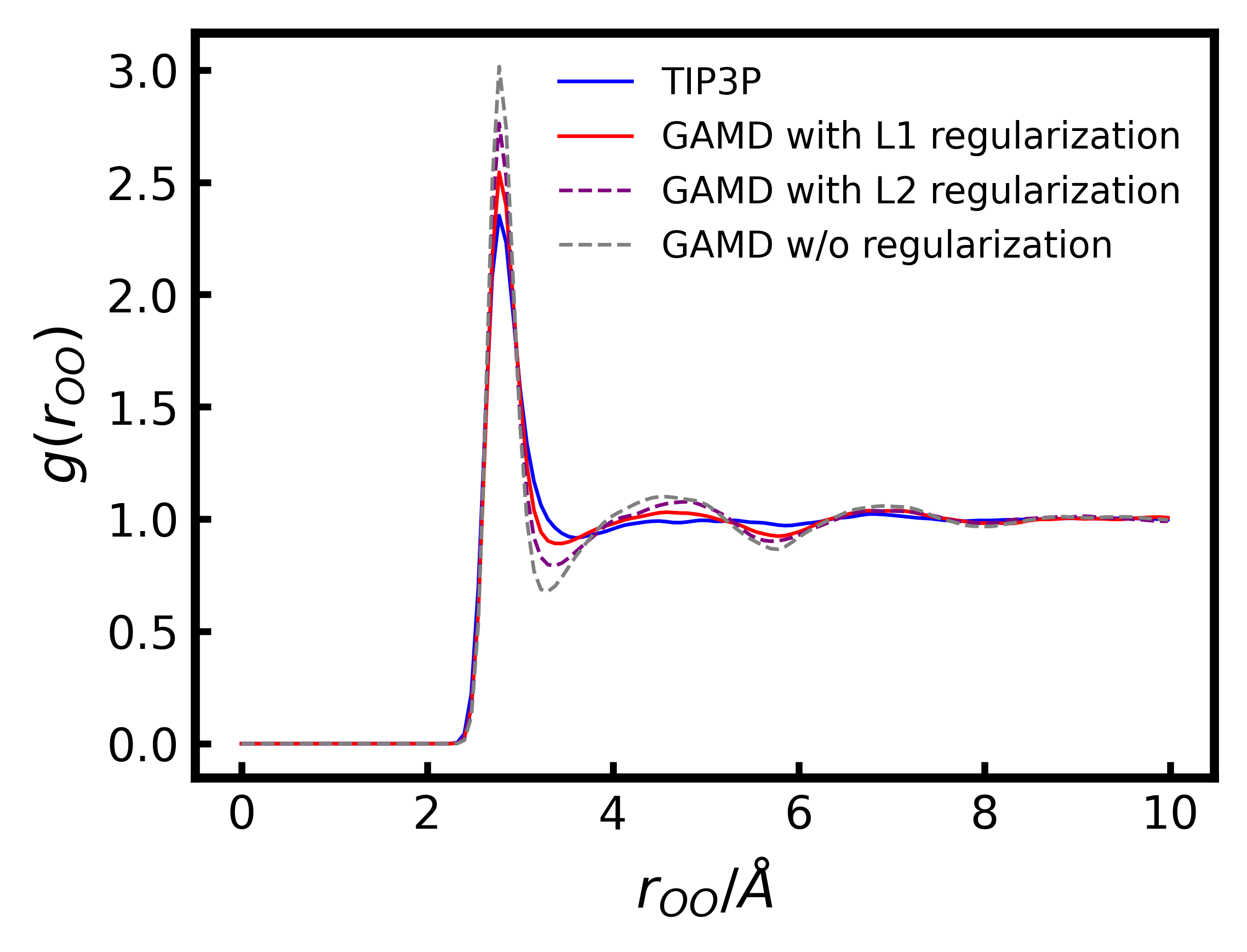
Figure 2: Comparison of models trained under different conditions. We measure the Oxygen-Oxygen RDF of water molecules’ trajectories generated from OpenMM’s TIP3P model and GAMD models trained using: 1.L1 regularization; 2.L2 regularization; 3.Without regularization.

As shown in Figure 2, the radial distribution functions (RDF) of the models trained with L2 regularization and without regularization have much sharper peaks and larger gaps compared to the ground truth, while there is a smaller gap between the RDF in the ground truth and GAMD trained under L1 regularization. This indicates that with L1 regularization the predicted forces have greater agreement with the ground truth and molecules are more uniformly distributed. Also, it demonstrates that imposing L1 regularization can effectively suppress unnecessary long-range message passing especially when there are multiple types of interaction with different influence ranges in the system.

Training strategy

We randomly split all datasets into train/test set with $90/10$ ratio. For the data generated from classical MD methods, the whole dataset contains $10,000$ snapshots of input (i.e. positions) and target (i.e. forces), where $9,000$ are used for training. For RPBE-D3 data based on DFT calculation, the whole dataset contains $6,518$ train snapshots and $723$ test snapshots.

Before calculating the loss, we normalize the ground truth forces, such that it has a zero mean and unit variance. We optimize the model using the Adam optimizer ⁸⁰, with an exponential learning rate scheduler that diminishes learning rate from $\alpha=3\times 10^{-4}$ to $\alpha=1\times 10^{-7}$. For data derived from classical MD, we train the model for 300k gradient updates. For DFT-based data, as its configurations are more diverse and complex than classical MD generated data, we train the model for 650k gradient updates.

Model implementation

We implement all the learnable functions described in the previous section as MLPs with three layers, using Gaussian Error Linear Units (GELUs)⁸¹ as non-linear activation function. For GAMD trained on DFT data, the embedding size of the network is 256, and the number of message passing layers is 5. For GAMD trained on MD data, the embedding size is 128, and the number of message passing layers is 4. On the DFT dataset, we do not use bond information as an edge feature as it is not available in the dataset. Following Schütt et al. ⁴⁴, we use Gaussian radial basis function to expand the interatomic distance before inputting into the edge encoder (Equation (1)). We found this resulted in a minor performance change on the investigated molecular systems. More details on the model’s architecture and ablation study on architectural choices can be found in the Supplementary Information.

3.4 Benchmark setting

To compare GAMD’s performance with other classical force calculation methods, we simulate the water system with different sizes using GAMD, OpenMM, and LAMMPS. As GAMD only modifies the force evaluation part of every step in the MD simulation, we exclude the running time of other calculations (e.g. chain propagation, position and velocity update) in the benchmark. All the benchmarks are run on a platform equipped with a single GTX-1080 Ti GPU and i7-8700k CPU. The benchmark results and discussion are presented in Section 4.3. Below we provide detailed configurations of benchmark for each package.

GAMD

Each force calculation step of GAMD comprises two parts, building the fixed radius graph and inference. Building the graph comprises updating the neighbor list, transforming the neighbor list into the adjacency matrix, and calculating the edge features between every pair of connected nodes (atoms). Note that in GAMD the rebuilding of the neighbor list and graph structure is performed when particles have traveled a distance larger than a threshold (heuristically we select this threshold as $d_{r}=r_{\text{cutoff}}/10$). We conduct a benchmark using GAMD with 4 message passing layers and an embedding size of 128, which contains $\approx$ 650k parameters.

OpenMM

To exclude the influence of other calculations involved in a single step of update, we run two simulations for each benchmark in the OpenMM. The first simulation runs in normal mode and in the second simulation, we remove all the forces defined in the system and run a dummy simulation with no forces being calculated. Then we estimate the time used to calculate forces in every step by: $t=t_{0}-t_{\text{dummy}}$, where $t_{0}$ denotes the time a normal simulation will take and $t_{\text{dummy}}$ denotes the time of dummy simulation.

LAMMPS

In LAMMPS, the force calculation in an update step mainly consists of four parts according to the description in the official document: Pair, Bond, Kspace and Neigh, where Pair denotes the evaluation of non-bonded forces, Bond denotes the evaluation of bonded interactions, Kspace denotes the evaluation of long-range interactions and Neigh denotes the neighbor list construction. We report the total time of Pair, Bond and Kspace at each step as the time used for force evaluation, and report Neigh as time used for searching neighbors. Visual Molecular Dynamics (VMD) ⁸² is used to create water box system for LAMMPS simulation.

4 Results and discussion

In this section, we present the results of GAMD on two common MD simulation systems - Lennard-Jones particles, and water molecules. We calculate the radial distribution function (RDF) to measure the spatial distribution of particles in each of the systems. The RDF $g(r)$ between two types of particles $A$ and $B$ is defined as:

$$g(r)=\frac{1}{N_{A}N_{B}}\sum_{i=1}^{N_{A}}\sum_{j=1}^{N_{B}}\langle\delta(||\mathbf{r}_{i}-\mathbf{r}_{j}||-r)\rangle$$ (10)

where $\langle\cdot\rangle$ denotes the ensemble average, $||\mathbf{r}_{i}-\mathbf{r}_{j}||$ denotes the Euclidean distance between two particles $i,j$, $r$ is the radius of the corresponding spherical shell, $N_{A}$ and $N_{B}$ denote the number of corresponding types of particles and $\delta$ filters particles’ distance not falling into this shell (which we implement as a Gaussian function). Furthermore, we validate the correctness of force prediction by comparing its angle and magnitude against ground truth.

4.1 Lennard-Jones system

We first investigate GAMD on a toy system consisting of liquid argon with non-bonded interatomic forces governed by Lennard-Jones (LJ) potential. This system comprises 258 argon atoms at 100 K and the non-bonded Van der Waals (VdW) potentials are approximated by LJ potentials. To evaluate the performance of GAMD in the prediction of interatomic LJ forces, we first compare the RDF of trajectories simulated using LJ potentials and the trained GAMD model (Figure 3(a)). This shows how the GAMD simulated trajectories preserve the spatial behavior of the classical MD’s trajectories.

Since the temperature is held constant in the NVT ensemble simulation, we can evaluate the temporal behavior of the results by comparing the temperature of the GAMD simulated system with the ground truth. Both of the simulations are initialized by sampling velocities from Boltzmann distribution with the temperature set to 100K, and they reach equilibrium after a few transient steps under the regulation of Nosé–Hoover chain thermostat with collision frequency: $25.0/ps$. Under the regulation by a thermostat, the trained model can successfully equilibrate to the target temperature (Figure 3(b)).

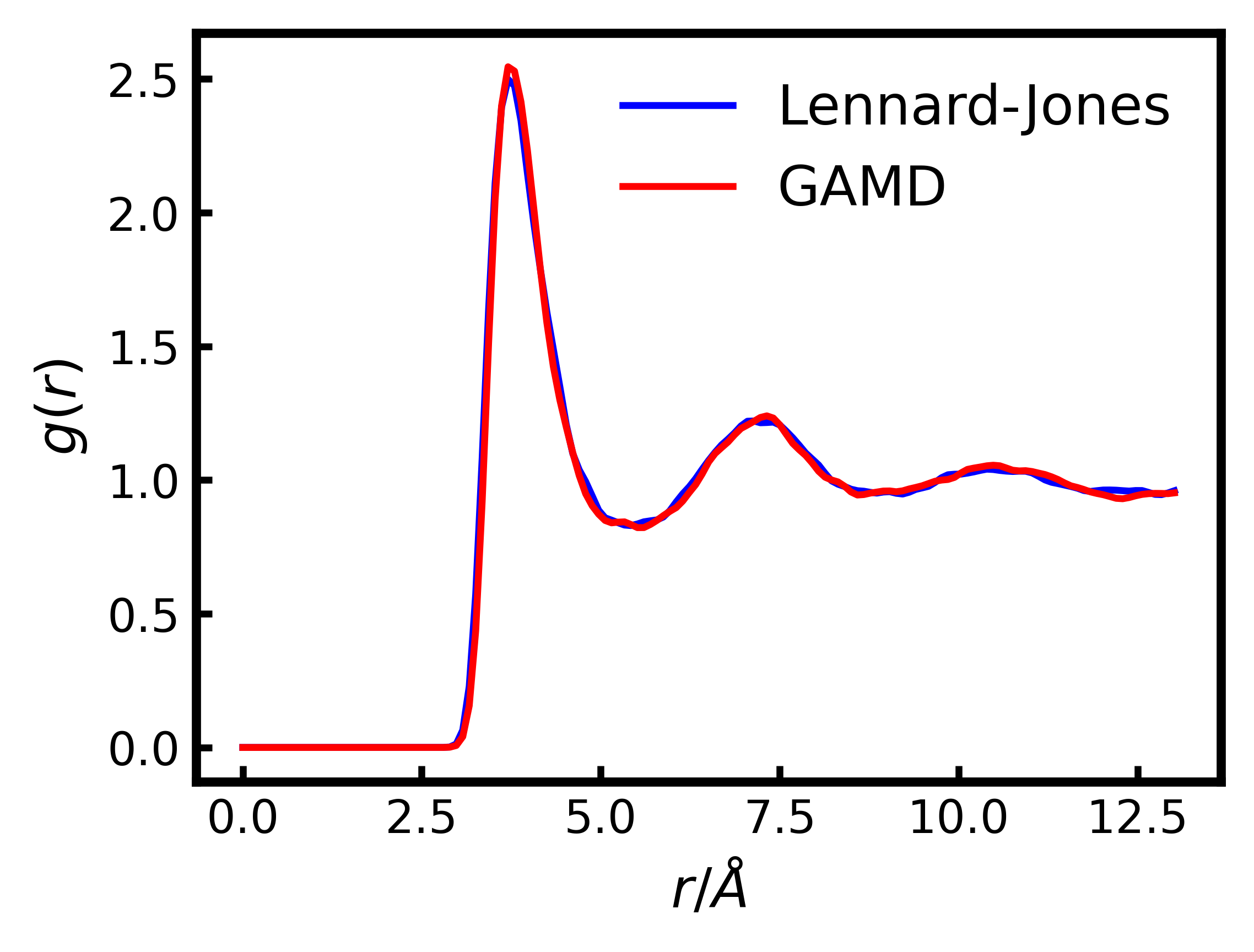
(a) RDF for particles in the Lennard-Jones system.

(b) Temperature trend of NVT ensemble in the Lennard-Jones system.

Figure 3: Comparison of GAMD generated trajectory with the ground truth Lennard-Jones system.

The rotation-covariant predicted forces are also compared directly in terms of both direction and magnitude with the ground truth LJ forces calculated in the MD simulations. By comparing $\cos\left<\hat{\mathbf{F}},\mathbf{F}\right>$ between the predicted and ground truth forces, we observe that more than $95\%$ of the predicted forces have $\cos\left<\hat{\mathbf{F}},\mathbf{F}\right>>0.995$. The mean absolute error (MAE), root mean squared error (RMSE), relative error, and force direction’s agreement on the test set are reported in Table 1. The relative error is evaluated as the ratio of mean absolute error to the mean L2 norm of the ground truth forces $\mathbf{F}$: $<\left|\mathbf{F}-\hat{\mathbf{F}}\right|>/<\left||\mathbf{F}|\right|_{2}>$. Figure 4 describes the agreement between the predicted forces and the ground truth LJ forces.

Ground Truth	Test snapshots	MAE ($meV/$\mathrm{\SIUnitSymbolAngstrom}$$)	RMSE ($meV/$\mathrm{\SIUnitSymbolAngstrom}$$)	$\cos<\hat{\mathbf{F}},\mathbf{F}>$	Relative error
Lennard Jones 73	1000	0.266 $\pm$ 0.030	0.427 $\pm$ 0.119	0.997	0.61% $\pm$ 0.07%

Table 1: Quantitative analysis of force accuracy. The standard deviation is measured by comparing the statistics within a single snapshot to the whole test dataset.

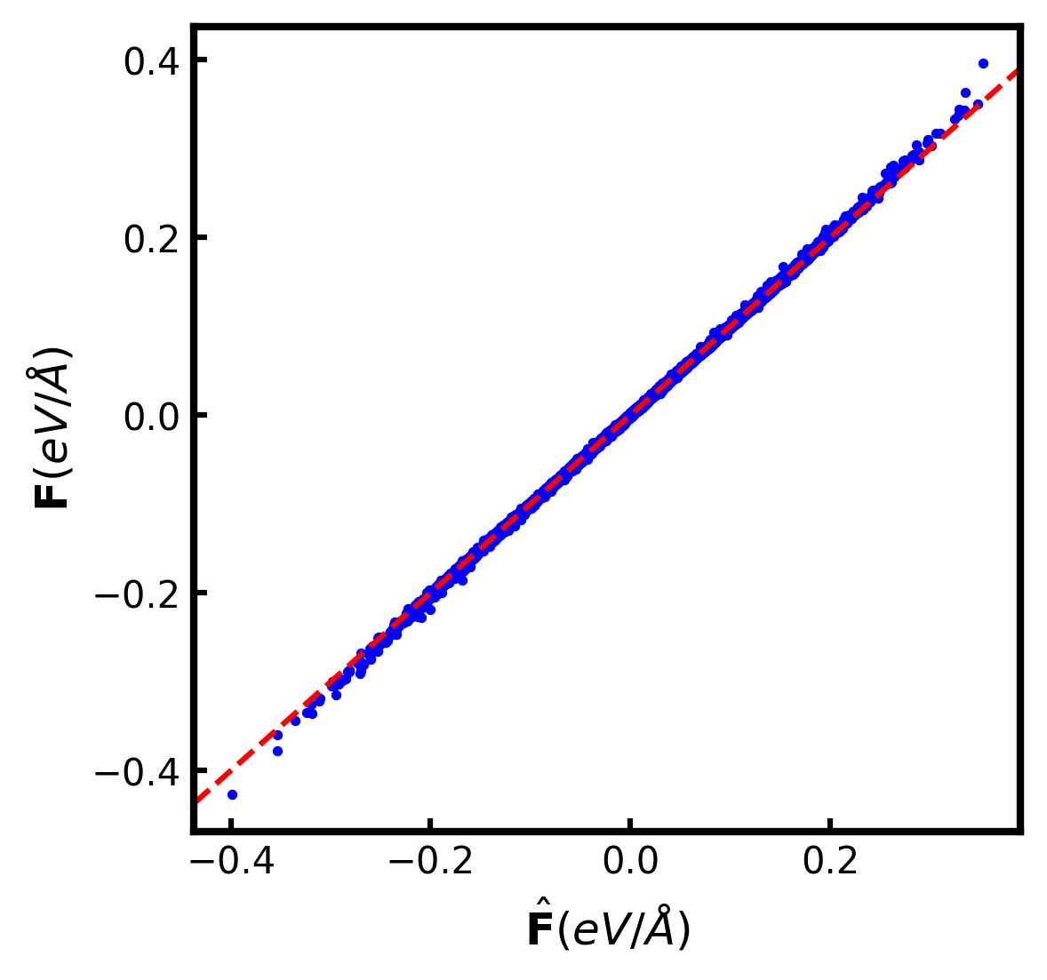
Figure 4: Forces derived from Lennard-Jones potential versus GAMD predicted forces. $\mathbf{F}$ denotes ground truth forces, $\hat{\mathbf{F}}$ denotes GAMD’s prediction.

4.2 Water system

In the second experiment, we apply GAMD on a system with water molecules, where interactions between particles are more complex and more types of particles are involved in the dynamics. Water molecules are ubiquitous solvents in a variety of molecular systems and their dynamic properties are of great importance. There is a wide array of works employing machine learning methods, especially neural networks to parametrize the potential energy of water molecules and study their interaction⁶⁵, ⁸³, ⁶⁶, ⁶⁷, ⁸⁴, ⁸⁵. In this work, we train and investigate GAMD using data derived from three different force models for water molecules - TIP3P ⁷⁴, TIP4P-Ew ⁷⁵ and DFT calculation based on revised Perdew–Burke–Ernzerhof functional (RPBE)^{78, 66}. Note that when training on the four-site model’s data, GAMD still adopts a three-site setting, where the forces of fictitious sites are not used. In these experiments, the model should be able to learn not only the non-bonded Van der Waals forces but also electrostatic forces due to the charges assigned to different types of atoms in a water molecule. Moreover, the model should handle two types of atoms, defined as node features, with different potentials and charges along with bonded and non-bonded interactions in and between molecules.

We run the MD simulation using GAMD on a cubic box (2 nanometers each edge with periodic boundary) with 258 water molecules of 300K temperature. Similar to the Lennard-Jones experiment, we investigate the RDF curves to evaluate the spatial behavior of the simulated trajectories using GAMD’s predicted forces. In general, GAMD can learn to predict forces from different data sources. The plotted RDF curve of Hydrogen-Hydrogen, Oxygen-Oxygen, and Oxygen-Hydrogen element pairs show the consistency of the GAMD’s trajectories with different reference models’ simulated trajectories (Figure 5, 6). In addition, as shown in Figure  7, the trajectory from GAMD trained on RPBE data has spatial structures that are consistent with experimental data.

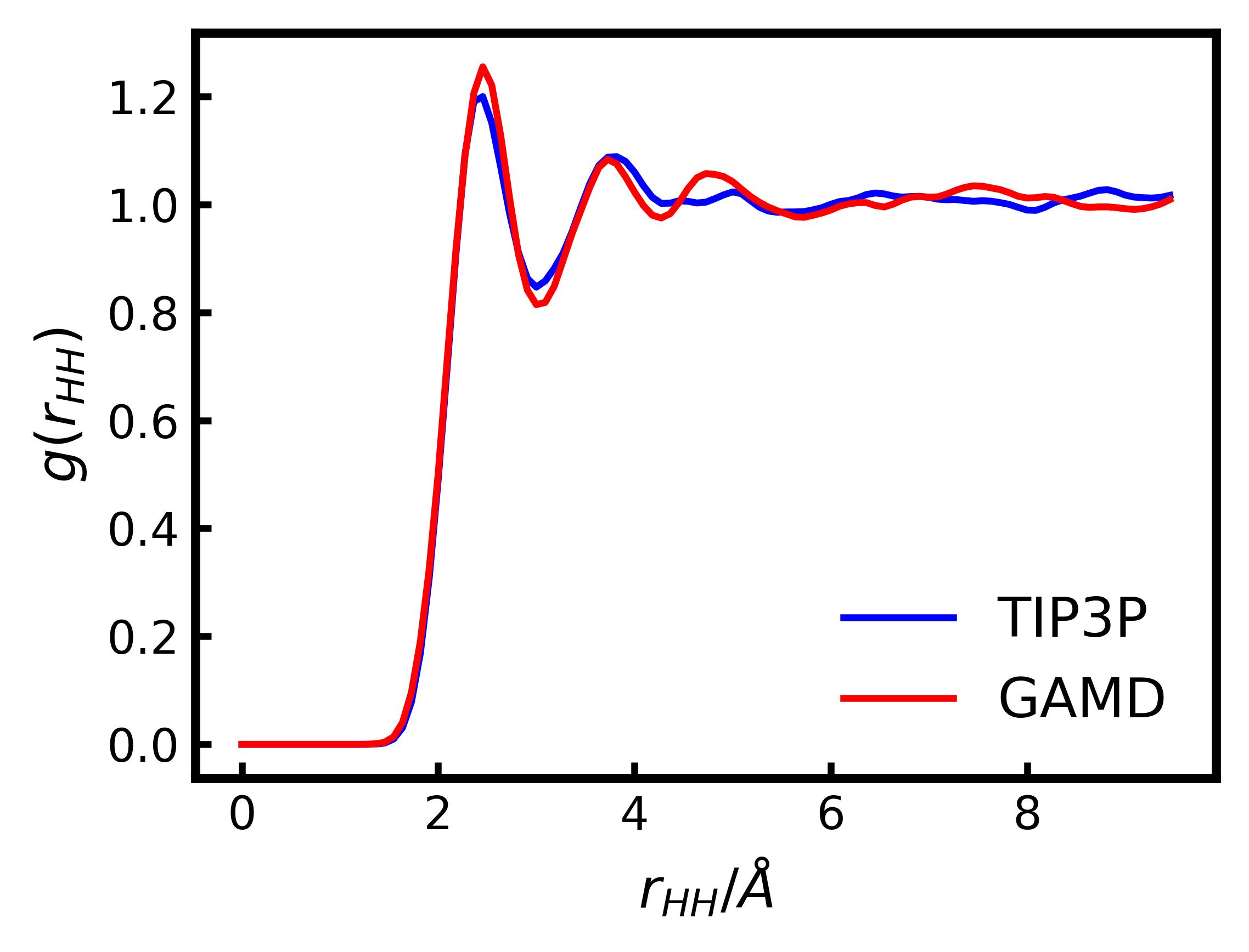
(a) Hydrogen-Hydrogen

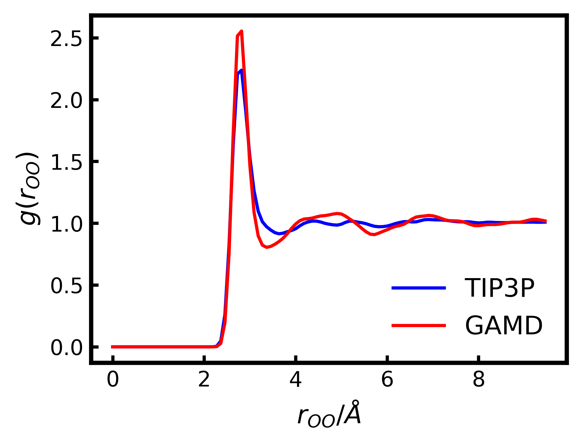
(b) Oxygen-Oxygen

(c) Oxygen-Hydrogen

Figure 5: Radial distribution function of GAMD (trained on TIP3P⁷⁴ data).

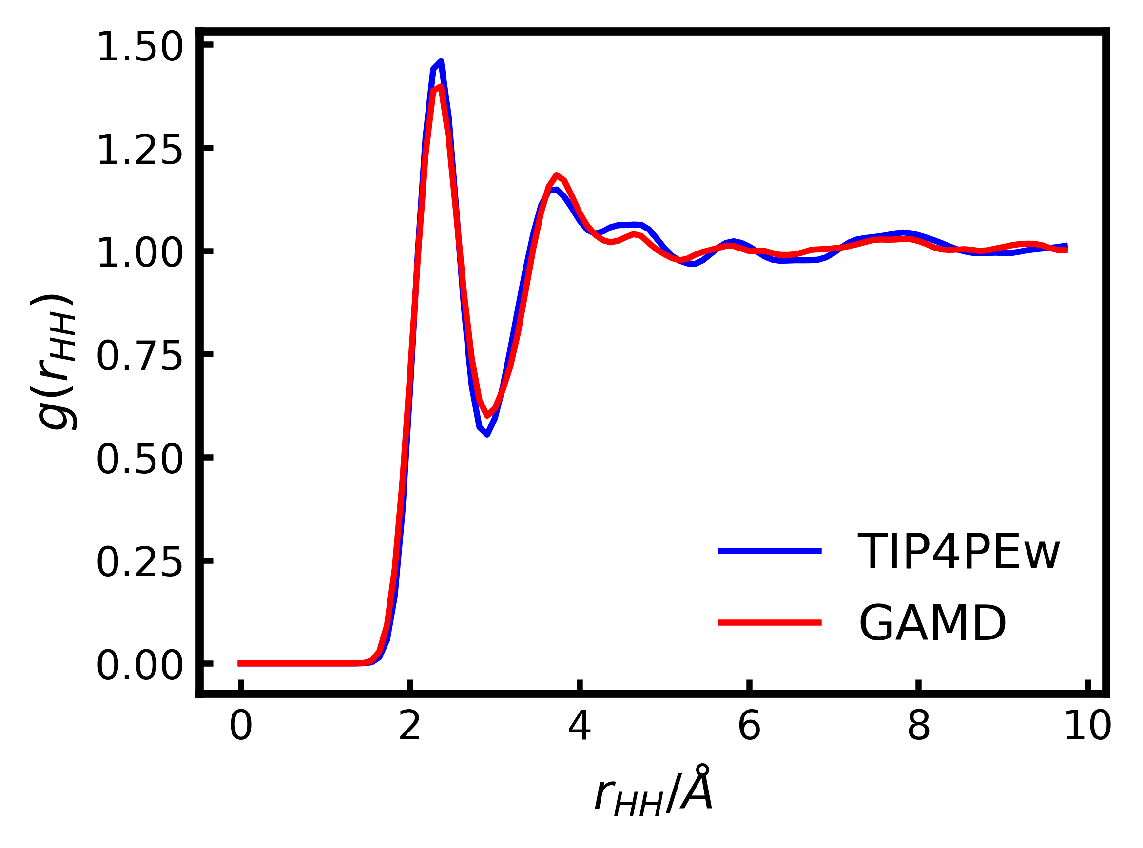
(a) Hydrogen-Hydrogen

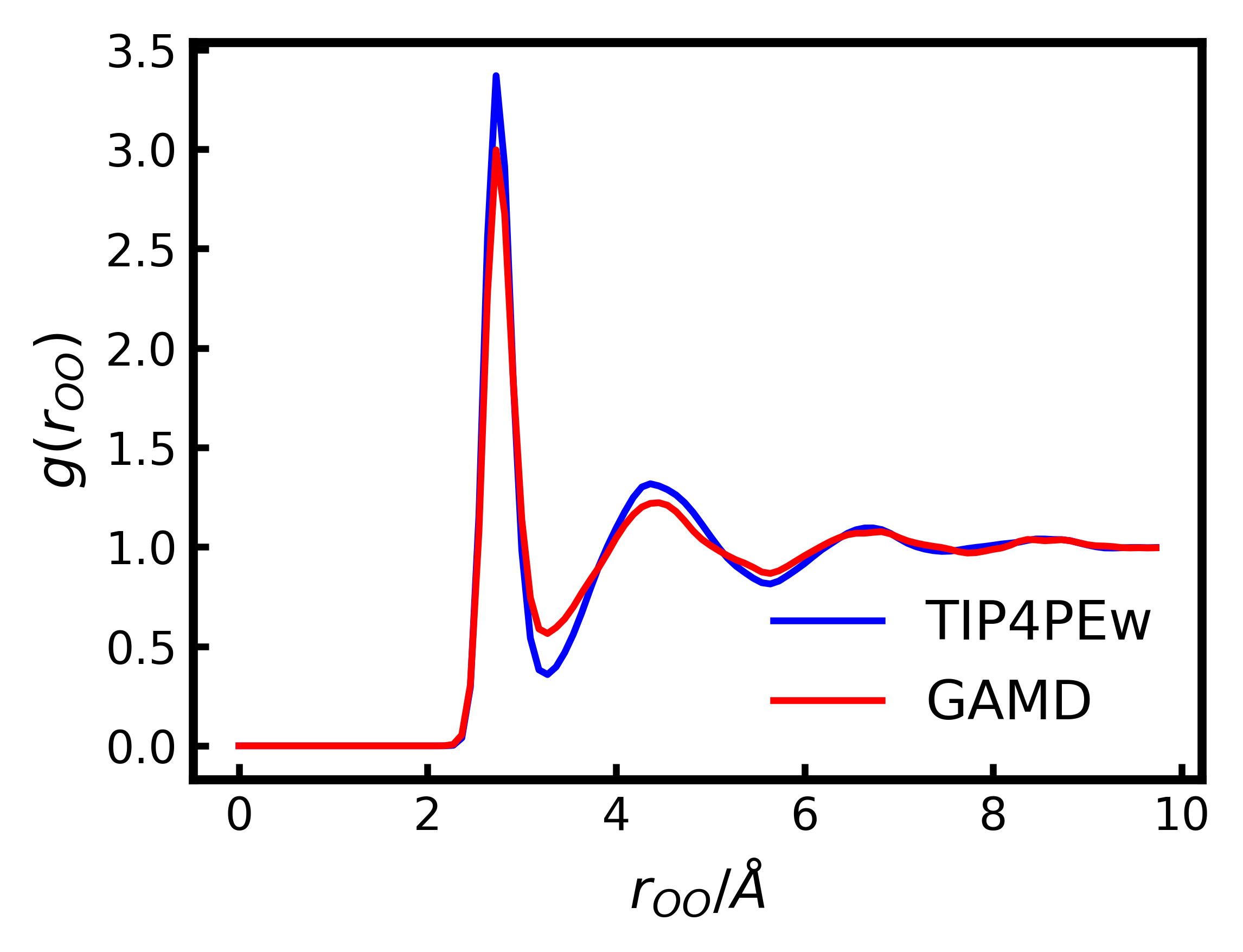
(b) Oxygen-Oxygen

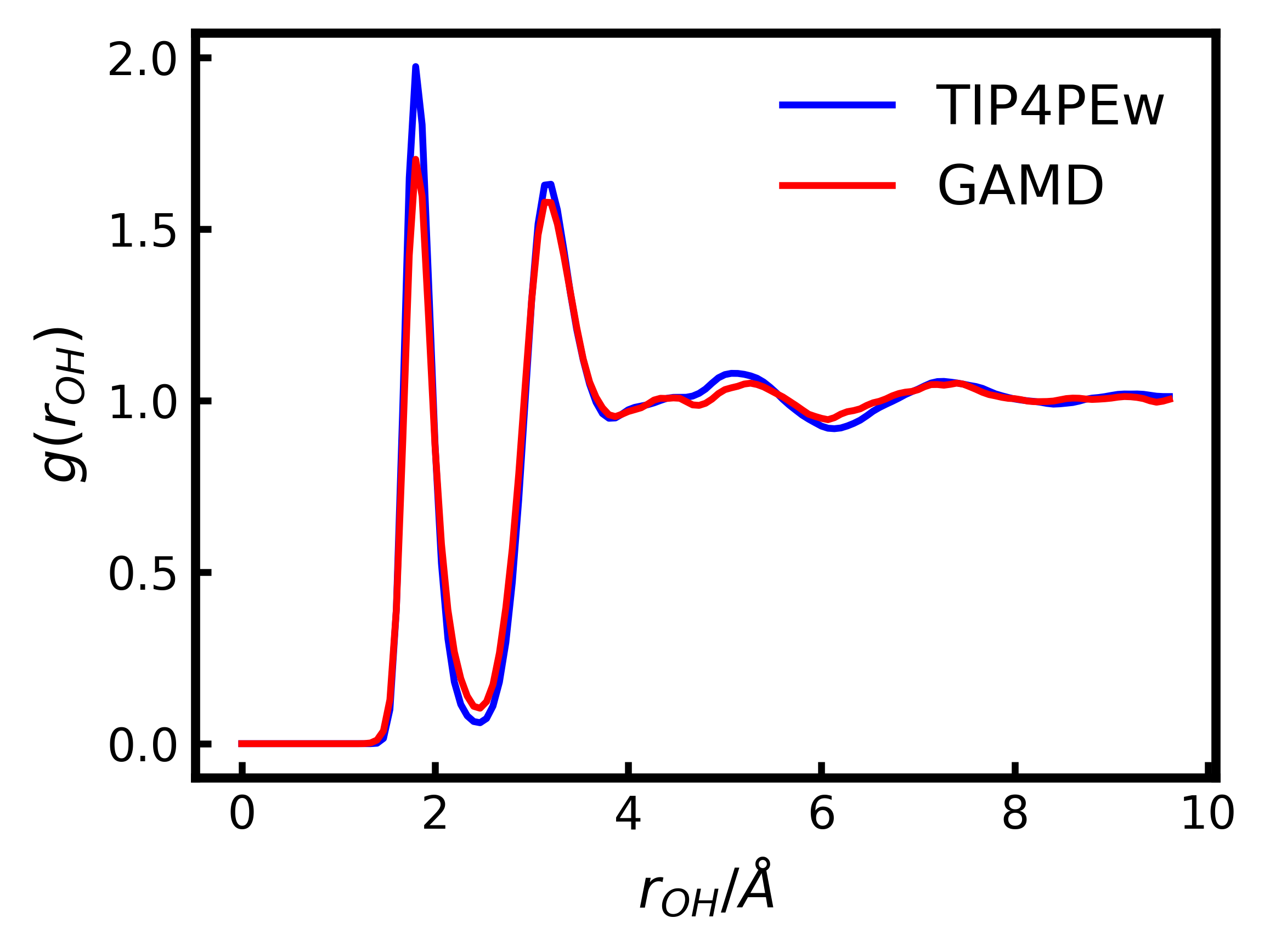
(c) Oxygen-Hydrogen

Figure 6: Radial distribution function of GAMD (trained on TIP4P-Ew⁷⁵ data).

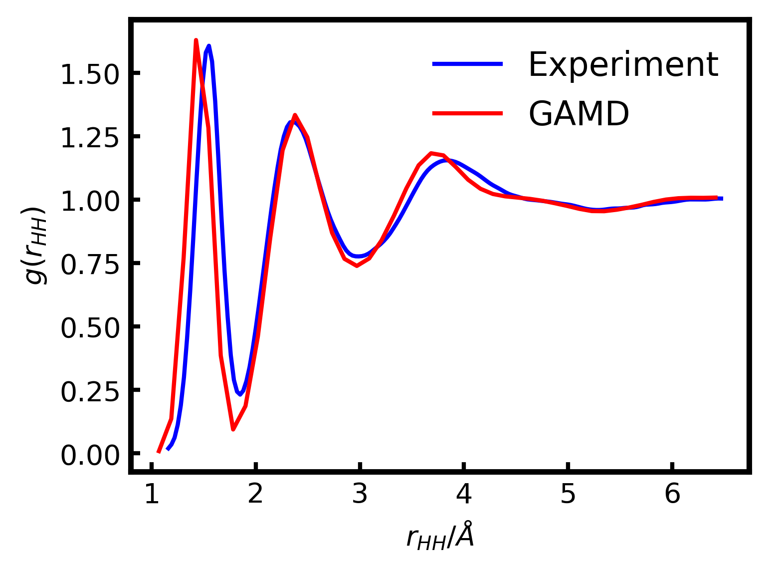
(a) Hydrogen-Hydrogen

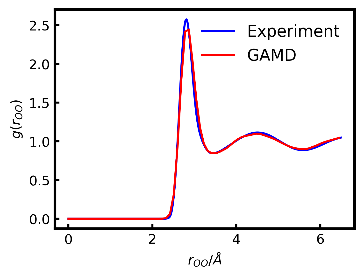
(b) Oxygen-Oxygen

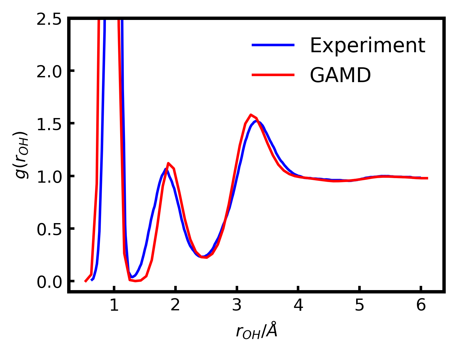
(c) Oxygen-Hydrogen

Figure 7: Radial distribution function of GAMD (trained on RPBE-D3⁶⁶, ⁷⁸, ⁷⁹ data). $X$-axis is truncated according to the corresponding experimental data. The experimental RDF data collection is taken from Cheng ⁸⁶. The original Hydrogen-Hydrogen RDF is from Chen et al. ⁸⁷, Oxygen-Oxygen RDF is from Skinner et al. ⁸⁸ and Oxygen-Hydrogen RDF is from Soper ⁸⁹.

In addition to the evaluation based on the spatial behavior of the simulated trajectories, we can directly compare GAMD’s predicted atomic forces with the forces derived from different force models by studying the predicted forces of GAMD trained on different data sources. Agreement in the direction of the forces is evaluated by comparing the $\cos\left<\hat{\mathbf{F}},\mathbf{F}\right>$ between the direction of predicted and reference forces. It has been observed that for models trained on empirical forcefields, more than $95\%$ of the predictions, $\cos\left<\hat{\mathbf{F}},\mathbf{F}\right>$ is of agreement above $0.995$ and $0.980$ for model trained on DFT data. Quantitative evaluation of errors of the predictions is reported in Table 2. Figure 8 depicts the alignment between predicted forces in each direction with the forces derived from different force models.

Ground Truth	Test snapthots	MAE ($meV/$\mathrm{\SIUnitSymbolAngstrom}$$)	RMSE ($meV/$\mathrm{\SIUnitSymbolAngstrom}$$)	$\cos<\hat{\mathbf{F}},\mathbf{F}>$	Relative error
TIP3P 74	1000	11.26 $\pm$ 0.84	15.16 $\pm$ 1.16	0.997	1.16% $\pm$ 0.09%
TIP4P-Ew 75	1000	13.86 $\pm$ 1.44	19.16 $\pm$ 4.47	0.999	1.29% $\pm$ 0.13%
RPBE-D3 66	723	24.28 $\pm$ 16.80	35.39 $\pm$ 23.09	0.986	1.47% $\pm$ 1.02%

Table 2: Quantitative analysis of force accuracy

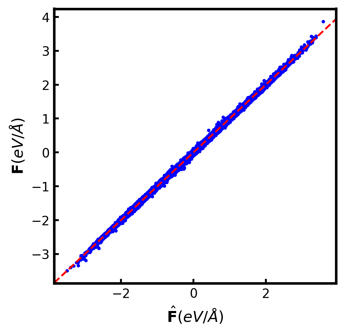
(a) GAMD trained on
TIP3P

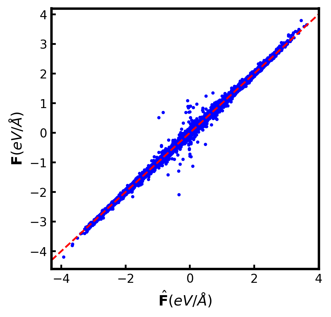
(b) GAMD trained on
TIP4P-Ew

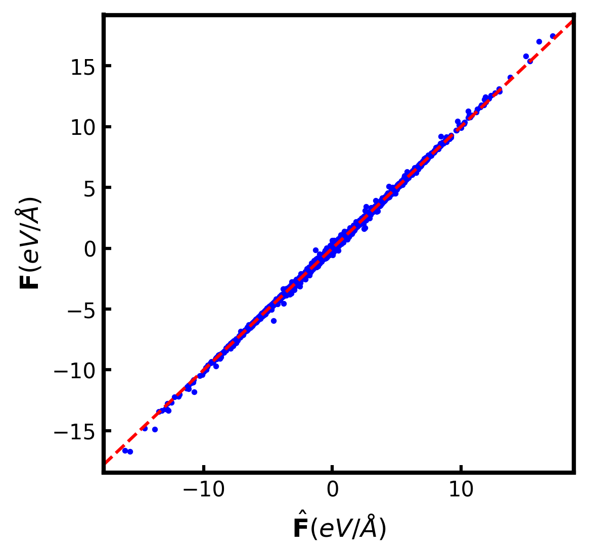
(c) GAMD trained on
RPBE-D3

Figure 8: Forces derived from different water potential models versus GAMD predicted forces. $\mathbf{F}$ denotes ground truth forces, $\hat{\mathbf{F}}$ denotes GAMD’s prediction.

Since forces in GAMD are not derived from potential energy surface, it does not conserve the potential energy of the system. Therefore GAMD requires thermostats to regulate the velocity during simulation. We study the temporal behavior and sensitivity of GAMD by using different thermostats to run NVT simulations. We test GAMD with different collision/dampening coefficients on Nosé–Hoover thermostat⁷⁶ and Langevin thermostat with BAOAB scheme⁹⁰. The temperature trends of GAMD trained on different water force models are shown in Figure 9, 10, 11. It is observed that GAMD cannot equilibrate under the NVE ensemble given its non-conserving property. When a relatively passive thermostat is applied, GAMD’s equilibrium will deviate from the target heat equilibrium. The models trained on TIP3P and TIP4P-Ew MD data are less sensitive to the intensity of the thermostat and can equilibrate to the target temperature with collision/dampening coefficient $\geq 5.0/ps$. The model trained on DFT data is more sensitive to this coefficient and requires more aggressive thermostat to maintain the target temperature. We hypothesize the main reason is that DFT training data encompasses a much diverse range of structures from low energy to high energy while MD data mostly consist of structures simulated around 300K temperature.

(a) Nosé–Hoover thermostat

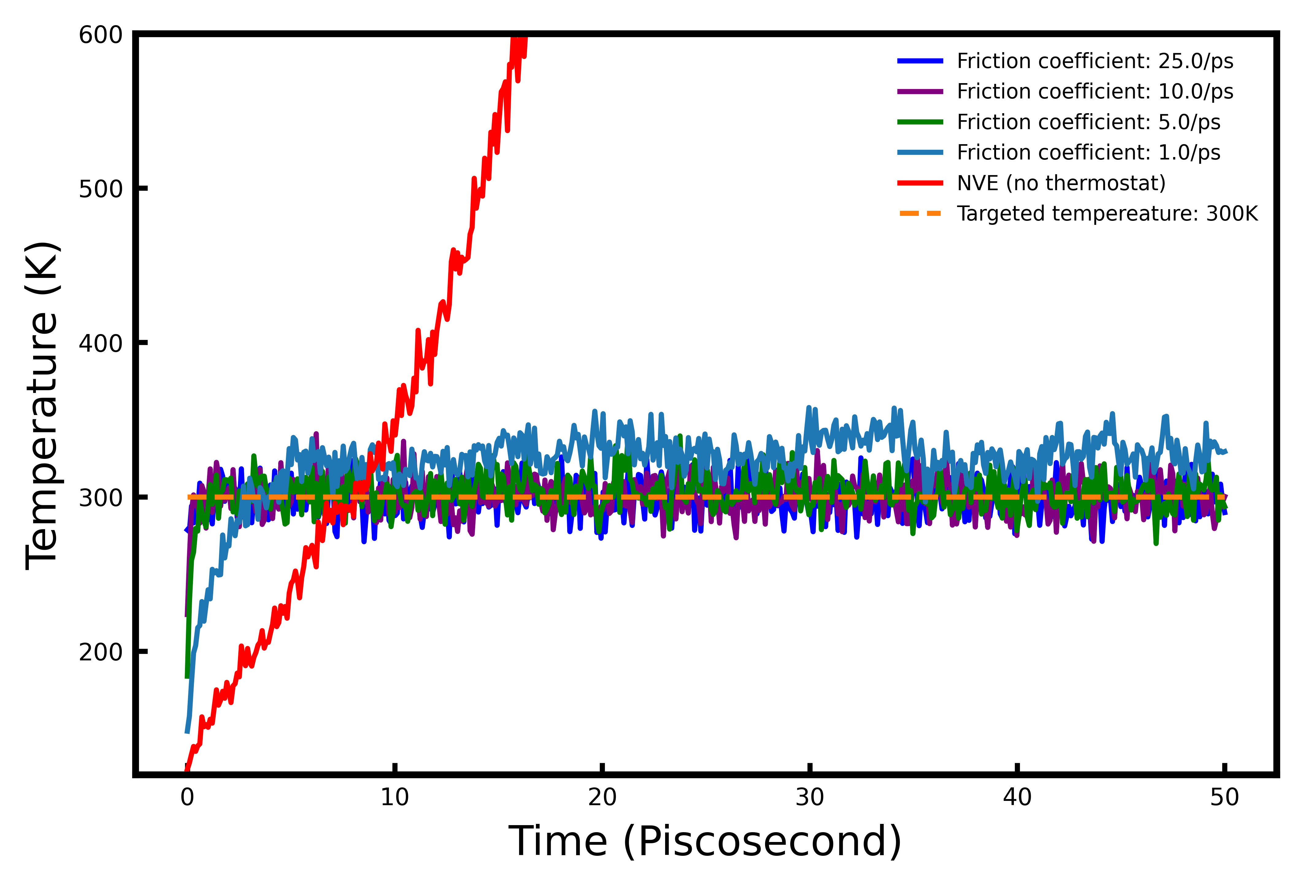
(b) Langevin thermostat

Figure 9: GAMD trained on TIP3P data.

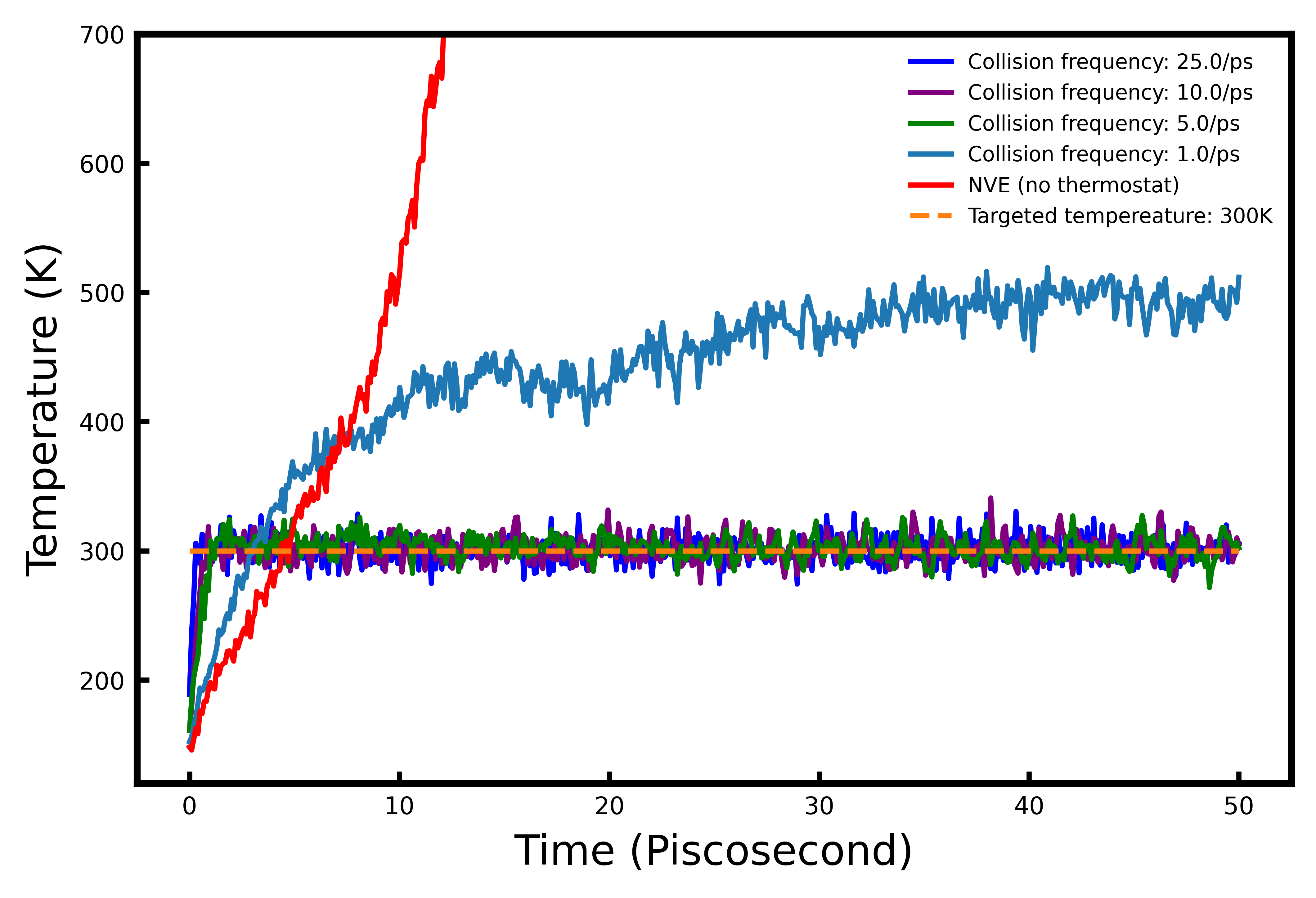
(a) Nosé–Hoover thermostat

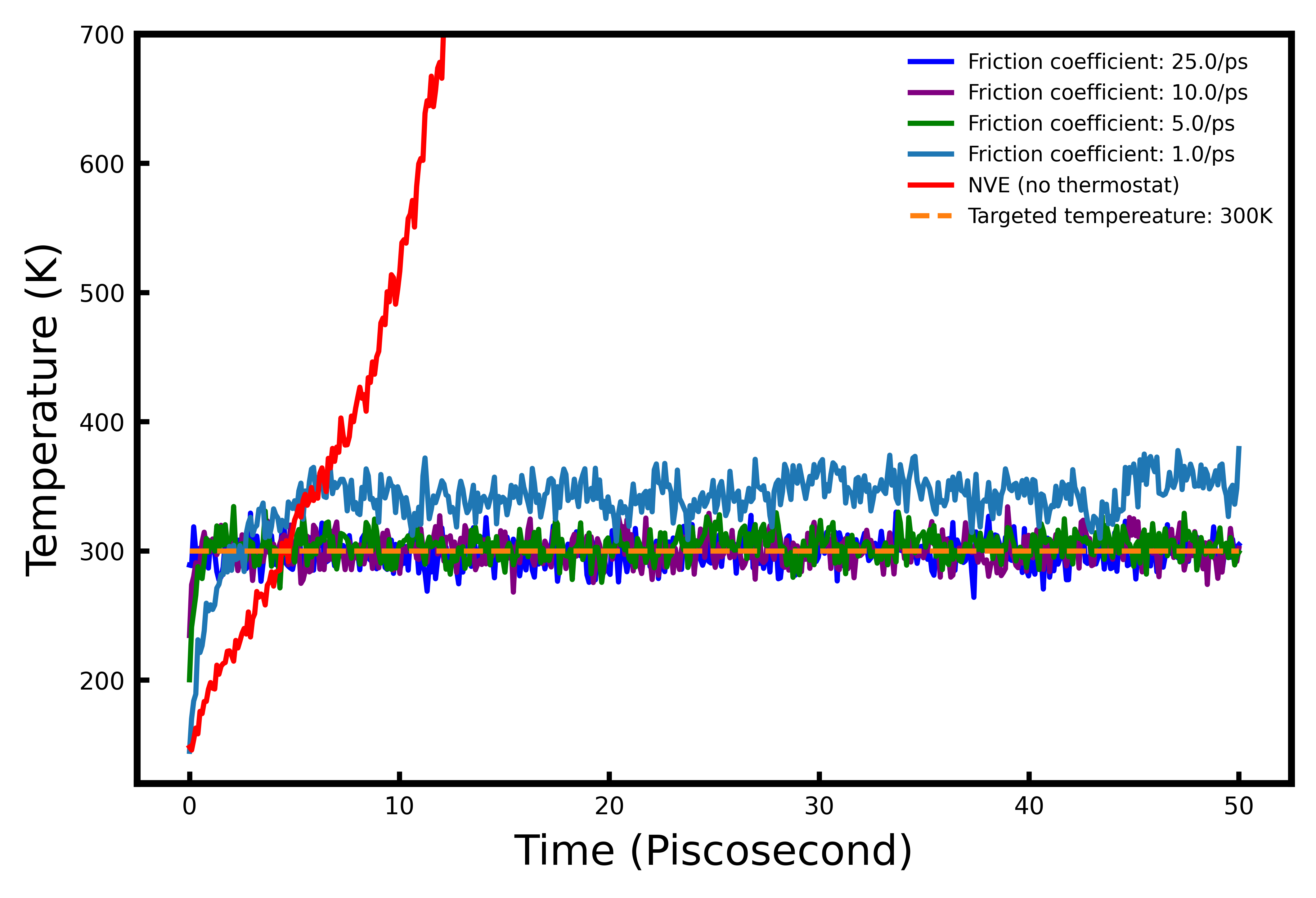
(b) Langevin thermostat

Figure 10: GAMD trained on TIP4P-Ew data.

(a) Nosé–Hoover thermostat

(b) Langevin thermostat

Figure 11: GAMD trained on RPBE data.

4.3 Scalability and Speed

Model	Molecule number	Box size (nm)	Time (ms) per force calculation step
			OpenMM	GAMD		LAMMPS
				Neighbor	Force Eval	Neighbor	Force Eval
3-site	258	2	0.192	2.962	4.063	0.001	0.754
	887	3	0.363	3.240	4.089	0.004	3.749
	2094	4	0.644	3.745	4.143	0.008	4.114
	4085	5	1.310	4.445	4.035	0.010	5.431
	13786	7.5	3.817	10.300	4.230	0.028	11.578
	24093	9	7.652	15.342	5.545	0.050	18.531
4-site	24093	9	7.848	-		0.056	28.164

Table 3: Quantitative comparison of force calculation speed on the Water box of different scales. In GAMD and LAMMPS, the time for each force evaluation is decomposed into two parts and reported separately. Neighbor denotes the time needed for updating the neighbor list (building graph and calculating edge features in GNN). Force Eval denotes the time to evaluate the net per-atom forces based on the neighbor list. GAMD adopts a 3-site setting for all of the calculations. The classical MD methods tested are TIP3P⁷⁴ and TIP4P-Ew⁷⁵.

We compare our model to two high-performance MD packages, OpenMM and LAMMPS, on the water box under multiple scales, ranging from 2 nanometers to 9 nanometers. The major bottleneck of current GAMD’s implementation is neighbor lists’ update and graph construction. The neighbor list update and graph construction in GAMD are based on JAX-MD, JAX, and DGL’s sparse matrix operation, which are optimized for machine learning workloads and are generally slower than customized CUDA neighbor-search routines used by MD packages. This results in the noticeable gap between the time of neighbor list update (including adjacency matrix assembling) in GAMD and counterparts in other MD packages. Despite this factor, GAMD still has a competitive computing efficiency (as shown in Table 3) at the large-scale simulation which is of great importance in practical problems ⁹¹. Since GAMD predicts forces directly by a set of MLPs which can be efficiently parallelized on the GPU, its actual force evaluation speed is faster than classical MD methods. We believe that with a more optimized implementation of the neighbor list data structure, GAMD’s performance can be further improved.

In comparision to classical MD simulation methods and DFT calculation, GAMD offers benefits in the following aspects. First, GAMD does not require explicit evaluation of energy and its gradient, instead, it directly predicts the net per-particle forces. Hence GAMD can learn the forcefield directly from observed data without any prior knowledge of the underlying energy equation. Second, GAMD does not require neighbor selection and energy accumulation based on different types of interactions (e.g. bonded interaction usually happened within a local region while non-bonded interaction happened between long-range particles). This reduces the computations needed in each step of simulation especially when there are multiple kinds of interactions in the system.

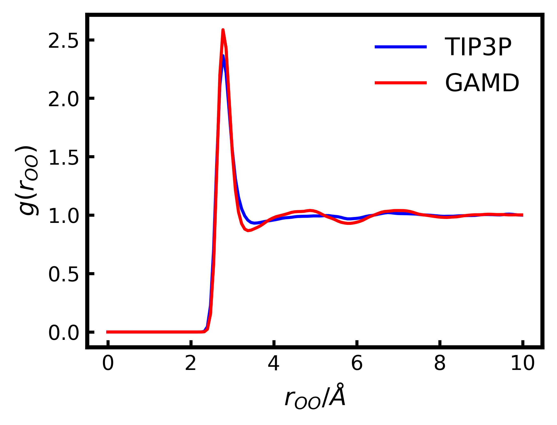
(a) Box size: $3~{}nm$

(b) Box size: $6~{}nm$

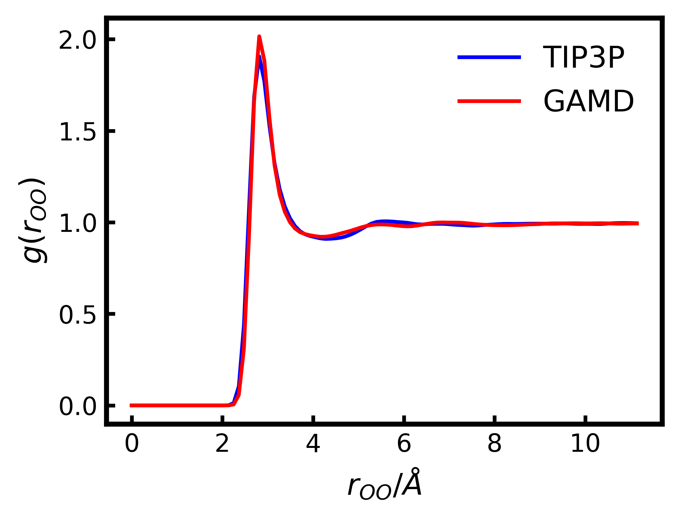
(c) Box size: $9~{}nm$

Figure 12: Radial distribution function for Oxygen-Oxygen distance in the water boxes of different sizes. (All the RDF plots are cutoff at $\sim 10$\mathrm{\SIUnitSymbolAngstrom}$$)

Figure 13: Relative error of force prediction on different sizes of water boxes. Error is measured and averaged on each simulation sequence of specific resolution.

Furthermore, GAMD is a supervised machine learning model in essence, but its scalability is not limited by the scale of training data. We find that GAMD can learn scale-agnostic dynamics and generalize well to much larger systems. Figure 12 and Figure 13 show that GAMD trained on a water box with 258 water molecules can be scaled up to a water box with much more molecules (about 100 times larger) without compromising accuracy. This demonstrates the scalability of the model and broadens the range of the problems where GAMD can operate.

5 Conclusion

A Graph Neural Networks Accelerated Molecular Dynamics model (GAMD) is presented. GAMD provides a data-driven framework that can predict atomic forces directly without explicitly calculating energy and does not require hand-designed molecular fingerprints. As GAMD does not derive energy from potential energy surface, it does not conserve energy and requires a thermostat to regulate velocities. We have showcased the applications of GAMD on two typical molecular systems - Lennard-Jones particles and water molecules. We use GAMD to simulate these systems in an NVT ensemble, which generates trajectories that are consistent with existing classical MD methods and experimental data in terms of spatial distribution and equilibrium state. It has also been shown that GAMD can be scaled up to much larger systems without compromising accuracy. Furthermore, a comprehensive benchmark on GAMD and other production-level MD engines (LAMMPS, OpenMM) is conducted, which shows GAMD has competitive efficiency at large-scale simulation.

6 Data Availability Statements

The data and code that support the findings of this project can be found at: https://github.com/BaratiLab/GAMD.

This work is supported by the start-up fund provided by CMU Mechanical Engineering, United States. The authors would like to thank Zhonglin Cao for valuable comments.

References

- Hollingsworth and Dror 2018 Hollingsworth, S. A.; Dror, R. O. Molecular Dynamics Simulation for All. Neuron 2018, 99, 1129–1143
- Karplus and McCammon 2002 Karplus, M.; McCammon, J. A. Molecular dynamics simulations of biomolecules. Nature Structural Biology 2002, 9, 646–652
- Becke 2014 Becke, A. D. Perspective: Fifty years of density-functional theory in chemical physics. The Journal of Chemical Physics 2014, 140, 18A301
- Unke et al. 2020 Unke, O. T.; Koner, D.; Patra, S.; Käser, S.; Meuwly, M. High-dimensional potential energy surfaces for molecular simulations: from empiricism to machine learning. Machine Learning: Science and Technology 2020, 1, 013001
- Harrison et al. 2018 Harrison, J. A.; Schall, J. D.; Maskey, S.; Mikulski, P. T.; Knippenberg, M. T.; Morrow, B. H. Review of force fields and intermolecular potentials used in atomistic computational materials research. Applied Physics Reviews 2018, 5, 031104
- Paquet and Viktor 2015 Paquet, E.; Viktor, H. L. Molecular dynamics, monte carlo simulations, and langevin dynamics: a computational review. BioMed research international 2015, 2015, 183918–183918, 25785262[pmid]
- Dror et al. 2010 Dror, R. O.; Jensen, M.; Borhani, D. W.; Shaw, D. E. Exploring atomic resolution physiology on a femtosecond to millisecond timescale using molecular dynamics simulations. Journal of General Physiology 2010, 135, 555–562
- Chmiela et al. 2017 Chmiela, S.; Tkatchenko, A.; Sauceda, H. E.; Poltavsky, I.; Schütt, K. T.; Müller, K.-R. Machine learning of accurate energy-conserving molecular force fields. Science Advances 2017, 3
- Hu et al. 2021 Hu, W.; Shuaibi, M.; Das, A.; Goyal, S.; Sriram, A.; Leskovec, J.; Parikh, D.; Zitnick, C. L. ForceNet: A Graph Neural Network for Large-Scale Quantum Calculations. 2021
- Mailoa et al. 2019 Mailoa, J. P.; Kornbluth, M.; Batzner, S.; Samsonidze, G.; Lam, S. T.; Vandermause, J.; Ablitt, C.; Molinari, N.; Kozinsky, B. A fast neural network approach for direct covariant forces prediction in complex multi-element extended systems. Nature Machine Intelligence 2019, 1, 471–479
- Park et al. 2021 Park, C. W.; Kornbluth, M.; Vandermause, J.; Wolverton, C.; Kozinsky, B.; Mailoa, J. P. Accurate and scalable graph neural network force field and molecular dynamics with direct force architecture. npj Computational Materials 2021, 7, 73
- Husic et al. 2020 Husic, B. E.; Charron, N. E.; Lemm, D.; Wang, J.; Pérez, A.; Majewski, M.; Krämer, A.; Chen, Y.; Olsson, S.; de Fabritiis, G.; Noé, F.; Clementi, C. Coarse graining molecular dynamics with graph neural networks. The Journal of Chemical Physics 2020, 153, 194101
- Wang et al. 2019 Wang, J.; Olsson, S.; Wehmeyer, C.; Pérez, A.; Charron, N. E.; de Fabritiis, G.; Noé, F.; Clementi, C. Machine Learning of Coarse-Grained Molecular Dynamics Force Fields. ACS Central Science 2019, 5, 755–767
- Husic et al. 2020 Husic, B. E.; Charron, N. E.; Lemm, D.; Wang, J.; Pérez, A.; Majewski, M.; Krämer, A.; Chen, Y.; Olsson, S.; de Fabritiis, G.; Noé, F.; Clementi, C. Coarse graining molecular dynamics with graph neural networks. The Journal of Chemical Physics 2020, 153, 194101
- Unke et al. 2021 Unke, O. T.; Chmiela, S.; Gastegger, M.; Schütt, K. T.; Sauceda, H. E.; Müller, K.-R. SpookyNet: Learning force fields with electronic degrees of freedom and nonlocal effects. Nature Communications 2021, 12, 7273
- Noé et al. 2020 Noé, F.; Tkatchenko, A.; Müller, K.-R.; Clementi, C. Machine Learning for Molecular Simulation. Annual Review of Physical Chemistry 2020, 71, 361–390, PMID: 32092281
- Gkeka et al. 2020 Gkeka, P.; Stoltz, G.; Barati Farimani, A.; Belkacemi, Z.; Ceriotti, M.; Chodera, J. D.; Dinner, A. R.; Ferguson, A. L.; Maillet, J.-B.; Minoux, H.; Peter, C.; Pietrucci, F.; Silveira, A.; Tkatchenko, A.; Trstanova, Z.; Wiewiora, R.; Lelièvre, T. Machine Learning Force Fields and Coarse-Grained Variables in Molecular Dynamics: Application to Materials and Biological Systems. Journal of Chemical Theory and Computation 2020, 16, 4757–4775, PMID: 32559068
- Unke et al. 2021 Unke, O. T.; Chmiela, S.; Sauceda, H. E.; Gastegger, M.; Poltavsky, I.; Schütt, K. T.; Tkatchenko, A.; Müller, K.-R. Machine Learning Force Fields. 2021
- Botu et al. 2017 Botu, V.; Batra, R.; Chapman, J.; Ramprasad, R. Machine Learning Force Fields: Construction, Validation, and Outlook. The Journal of Physical Chemistry C 2017, 121, 511–522
- Li et al. 2017 Li, Y.; Li, H.; Pickard, F. C.; Narayanan, B.; Sen, F. G.; Chan, M. K. Y.; Sankaranarayanan, S. K. R. S.; Brooks, B. R.; Roux, B. Machine Learning Force Field Parameters from Ab Initio Data. Journal of Chemical Theory and Computation 2017, 13, 4492–4503, PMID: 28800233
- Chmiela et al. 2018 Chmiela, S.; Sauceda, H. E.; Müller, K.-R.; Tkatchenko, A. Towards exact molecular dynamics simulations with machine-learned force fields. Nature Communications 2018, 9, 3887
- Deringer et al. 2019 Deringer, V. L.; Caro, M. A.; Csányi, G. Machine Learning Interatomic Potentials as Emerging Tools for Materials Science. Advanced Materials 2019, 31, 1902765
- Behler 2016 Behler, J. Perspective: Machine learning potentials for atomistic simulations. The Journal of Chemical Physics 2016, 145, 170901
- Eshet et al. 2010 Eshet, H.; Khaliullin, R. Z.; Kühne, T. D.; Behler, J.; Parrinello, M. Ab initio quality neural-network potential for sodium. Phys. Rev. B 2010, 81, 184107
- Artrith et al. 2011 Artrith, N.; Morawietz, T.; Behler, J. High-dimensional neural-network potentials for multicomponent systems: Applications to zinc oxide. Phys. Rev. B 2011, 83, 153101
- Wang et al. 2018 Wang, H.; Zhang, L.; Han, J.; E, W. DeePMD-kit: A deep learning package for many-body potential energy representation and molecular dynamics. Computer Physics Communications 2018, 228, 178–184
- Artrith et al. 2017 Artrith, N.; Urban, A.; Ceder, G. Efficient and accurate machine-learning interpolation of atomic energies in compositions with many species. Phys. Rev. B 2017, 96, 014112
- Sanchez-Gonzalez et al. 2020 Sanchez-Gonzalez, A.; Godwin, J.; Pfaff, T.; Ying, R.; Leskovec, J.; Battaglia, P. W. Learning to Simulate Complex Physics with Graph Networks. Proceedings of the 37th International Conference on Machine Learning, ICML 2020, 13-18 July 2020, Virtual Event. 2020; pp 8459–8468
- Bapst et al. 2020 Bapst, V.; Keck, T.; Grabska-Barwińska, A.; Donner, C.; Cubuk, E. D.; Schoenholz, S. S.; Obika, A.; Nelson, A. W. R.; Back, T.; Hassabis, D.; Kohli, P. Unveiling the predictive power of static structure in glassy systems. Nature Physics 2020, 16, 448–454
- Battaglia et al. 2016 Battaglia, P.; Pascanu, R.; Lai, M.; Jimenez Rezende, D.; kavukcuoglu, k. Interaction Networks for Learning about Objects, Relations and Physics. Advances in Neural Information Processing Systems. 2016
- Bartók et al. 2017 Bartók, A. P.; De, S.; Poelking, C.; Bernstein, N.; Kermode, J. R.; Csányi, G.; Ceriotti, M. Machine learning unifies the modeling of materials and molecules. Science Advances 2017, 3
- Chen et al. 2019 Chen, C.; Ye, W.; Zuo, Y.; Zheng, C.; Ong, S. P. Graph Networks as a Universal Machine Learning Framework for Molecules and Crystals. Chemistry of Materials 2019, 31, 3564–3572
- Smith et al. 2017 Smith, J. S.; Isayev, O.; Roitberg, A. E. ANI-1: an extensible neural network potential with DFT accuracy at force field computational cost. Chem. Sci. 2017, 8, 3192–3203
- Christensen et al. 2020 Christensen, A. S.; Bratholm, L. A.; Faber, F. A.; Anatole von Lilienfeld, O. FCHL revisited: Faster and more accurate quantum machine learning. The Journal of Chemical Physics 2020, 152, 044107
- Zhang et al. 2018 Zhang, L.; Han, J.; Wang, H.; Car, R.; E, W. Deep Potential Molecular Dynamics: A Scalable Model with the Accuracy of Quantum Mechanics. Phys. Rev. Lett. 2018, 120, 143001
- Carbogno et al. 2008 Carbogno, C.; Behler, J.; Groß, A.; Reuter, K. Fingerprints for Spin-Selection Rules in the Interaction Dynamics of at Al(111). Phys. Rev. Lett. 2008, 101, 096104
- Behler 2011 Behler, J. Atom-centered symmetry functions for constructing high-dimensional neural network potentials. The Journal of Chemical Physics 2011, 134, 074106
- Behler and Parrinello 2007 Behler, J.; Parrinello, M. Generalized Neural-Network Representation of High-Dimensional Potential-Energy Surfaces. Phys. Rev. Lett. 2007, 98, 146401
- Behler 2017 Behler, J. First Principles Neural Network Potentials for Reactive Simulations of Large Molecular and Condensed Systems. Angewandte Chemie International Edition 2017, 56, 12828–12840
- Duvenaud et al. 2015 Duvenaud, D. K.; Maclaurin, D.; Iparraguirre, J.; Bombarell, R.; Hirzel, T.; Aspuru-Guzik, A.; Adams, R. P. Convolutional Networks on Graphs for Learning Molecular Fingerprints. Advances in Neural Information Processing Systems. 2015
- Kearnes et al. 2016 Kearnes, S.; McCloskey, K.; Berndl, M.; Pande, V.; Riley, P. Molecular graph convolutions: moving beyond fingerprints. Journal of Computer-Aided Molecular Design 2016, 30, 595–608
- Schütt et al. 2017 Schütt, K. T.; Arbabzadah, F.; Chmiela, S.; Müller, K. R.; Tkatchenko, A. Quantum-chemical insights from deep tensor neural networks. Nature Communications 2017, 8, 13890
- Unke and Meuwly 2019 Unke, O. T.; Meuwly, M. PhysNet: A Neural Network for Predicting Energies, Forces, Dipole Moments, and Partial Charges. Journal of Chemical Theory and Computation 2019, 15, 3678–3693, PMID: 31042390
- Schütt et al. 2017 Schütt, K. T.; Kindermans, P.-J.; Sauceda, H. E.; Chmiela, S.; Tkatchenko, A.; Müller, K.-R. SchNet: A continuous-filter convolutional neural network for modeling quantum interactions. 2017
- Lubbers et al. 2018 Lubbers, N.; Smith, J. S.; Barros, K. Hierarchical modeling of molecular energies using a deep neural network. The Journal of Chemical Physics 2018, 148, 241715
- Imbalzano et al. 2018 Imbalzano, G.; Anelli, A.; Giofré, D.; Klees, S.; Behler, J.; Ceriotti, M. Automatic selection of atomic fingerprints and reference configurations for machine-learning potentials. The Journal of Chemical Physics 2018, 148, 241730
- Pfaff et al. 2021 Pfaff, T.; Fortunato, M.; Sanchez-Gonzalez, A.; Battaglia, P. Learning Mesh-Based Simulation with Graph Networks. International Conference on Learning Representations. 2021
- Shlomi et al. 2021 Shlomi, J.; Battaglia, P.; Vlimant, J.-R. Graph neural networks in particle physics. Machine Learning: Science and Technology 2021, 2, 021001
- Li and Farimani 2022 Li, Z.; Farimani, A. B. Graph neural network-accelerated Lagrangian fluid simulation. Computers & Graphics 2022,
- Ogoke et al. 2020 Ogoke, F.; Meidani, K.; Hashemi, A.; Farimani, A. B. Graph Convolutional Neural Networks for Body Force Prediction. 2020
- Brandstetter et al. 2022 Brandstetter, J.; Worrall, D. E.; Welling, M. Message Passing Neural PDE Solvers. International Conference on Learning Representations. 2022
- de Avila Belbute-Peres et al. 2020 de Avila Belbute-Peres, F.; Economon, T. D.; Kolter, J. Z. Combining Differentiable PDE Solvers and Graph Neural Networks for Fluid Flow Prediction. 2020
- Xie and Grossman 2018 Xie, T.; Grossman, J. C. Crystal Graph Convolutional Neural Networks for an Accurate and Interpretable Prediction of Material Properties. Phys. Rev. Lett. 2018, 120, 145301
- Karamad et al. 2020 Karamad, M.; Magar, R.; Shi, Y.; Siahrostami, S.; Gates, I. D.; Barati Farimani, A. Orbital graph convolutional neural network for material property prediction. Phys. Rev. Materials 2020, 4, 093801
- Wang et al. 2021 Wang, Y.; Wang, J.; Cao, Z.; Farimani, A. B. MolCLR: Molecular Contrastive Learning of Representations via Graph Neural Networks. 2021
- Gilmer et al. 2017 Gilmer, J.; Schoenholz, S. S.; Riley, P. F.; Vinyals, O.; Dahl, G. E. Neural Message Passing for Quantum Chemistry. Proceedings of the 34th International Conference on Machine Learning. 2017; pp 1263–1272
- Klicpera et al. 2020 Klicpera, J.; Groß, J.; Günnemann, S. Directional Message Passing for Molecular Graphs. International Conference on Learning Representations. 2020
- Klicpera et al. 2020 Klicpera, J.; Giri, S.; Margraf, J. T.; Gunnemann, S. Fast and Uncertainty-Aware Directional Message Passing for Non-Equilibrium Molecules. ArXiv 2020, abs/2011.14115
- Schoenholz and Cubuk 2020 Schoenholz, S. S.; Cubuk, E. D. JAX M.D. A Framework for Differentiable Physics. Advances in Neural Information Processing Systems. 2020
- Doerr et al. 2021 Doerr, S.; Majewski, M.; Pérez, A.; Krämer, A.; Clementi, C.; Noe, F.; Giorgino, T.; De Fabritiis, G. TorchMD: A Deep Learning Framework for Molecular Simulations. Journal of Chemical Theory and Computation 2021, 17, 2355–2363, PMID: 33729795
- Schütt et al. 2019 Schütt, K. T.; Kessel, P.; Gastegger, M.; Nicoli, K. A.; Tkatchenko, A.; Müller, K.-R. SchNetPack: A Deep Learning Toolbox For Atomistic Systems. Journal of Chemical Theory and Computation 2019, 15, 448–455
- Wang et al. 2020 Wang, W.; Axelrod, S.; Gómez-Bombarelli, R. Differentiable Molecular Simulations for Control and Learning. ICLR 2020 Workshop on Integration of Deep Neural Models and Differential Equations. 2020
- Pukrittayakamee et al. 2009 Pukrittayakamee, A.; Malshe, M.; Hagan, M.; Raff, L. M.; Narulkar, R.; Bukkapatnum, S.; Komanduri, R. Simultaneous fitting of a potential-energy surface and its corresponding force fields using feedforward neural networks. The Journal of Chemical Physics 2009, 130, 134101
- Chanussot et al. 2021 Chanussot, L.; Das, A.; Goyal, S.; Lavril, T.; Shuaibi, M.; Riviere, M.; Tran, K.; Heras-Domingo, J.; Ho, C.; Hu, W.; Palizhati, A.; Sriram, A.; Wood, B.; Yoon, J.; Parikh, D.; Zitnick, C. L.; Ulissi, Z. Open Catalyst 2020 (OC20) Dataset and Community Challenges. ACS Catalysis 2021, 11, 6059–6072
- Morawietz and Behler 2013 Morawietz, T.; Behler, J. A Density-Functional Theory-Based Neural Network Potential for Water Clusters Including van der Waals Corrections. The Journal of Physical Chemistry A 2013, 117, 7356–7366, PMID: 23557541
- Morawietz et al. 2016 Morawietz, T.; Singraber, A.; Dellago, C.; Behler, J. How van der Waals interactions determine the unique properties of water. Proceedings of the National Academy of Sciences 2016, 113, 8368–8373
- Cheng et al. 2019 Cheng, B.; Engel, E. A.; Behler, J.; Dellago, C.; Ceriotti, M. Ab initio thermodynamics of liquid and solid water. Proceedings of the National Academy of Sciences 2019, 116, 1110–1115
- Ba et al. 2016 Ba, J. L.; Kiros, J. R.; Hinton, G. E. Layer Normalization. 2016
- He et al. 2015 He, K.; Zhang, X.; Ren, S.; Sun, J. Deep Residual Learning for Image Recognition. 2015
- Paszke et al. 2019 Paszke, A.; Gross, S.; Massa, F.; Lerer, A.; Bradbury, J.; Chanan, G.; Killeen, T.; Lin, Z.; Gimelshein, N.; Antiga, L.; Desmaison, A.; Kopf, A.; Yang, E.; DeVito, Z.; Raison, M.; Tejani, A.; Chilamkurthy, S.; Steiner, B.; Fang, L.; Bai, J.; Chintala, S. In Advances in Neural Information Processing Systems 32; Wallach, H., Larochelle, H., Beygelzimer, A., d'Alché-Buc, F., Fox, E., Garnett, R., Eds.; Curran Associates, Inc., 2019; pp 8024–8035
- Wang et al. 2019 Wang, M.; Zheng, D.; Ye, Z.; Gan, Q.; Li, M.; Song, X.; Zhou, J.; Ma, C.; Yu, L.; Gai, Y.; Xiao, T.; He, T.; Karypis, G.; Li, J.; Zhang, Z. Deep Graph Library: A Graph-Centric, Highly-Performant Package for Graph Neural Networks. arXiv preprint arXiv:1909.01315 2019,
- Eastman et al. 2017 Eastman, P.; Swails, J.; Chodera, J. D.; McGibbon, R. T.; Zhao, Y.; Beauchamp, K. A.; Wang, L.-P.; Simmonett, A. C.; Harrigan, M. P.; Stern, C. D.; Wiewiora, R. P.; Brooks, B. R.; Pande, V. S. OpenMM 7: Rapid development of high performance algorithms for molecular dynamics. PLOS Computational Biology 2017, 13, 1–17
- Lennard-Jones 1931 Lennard-Jones, J. E. Cohesion. Proceedings of the Physical Society 1931, 43, 461–482
- Jorgensen et al. 1983 Jorgensen, W. L.; Chandrasekhar, J.; Madura, J. D.; Impey, R. W.; Klein, M. L. Comparison of simple potential functions for simulating liquid water. The Journal of Chemical Physics 1983, 79, 926–935
- Horn et al. 2004 Horn, H. W.; Swope, W. C.; Pitera, J. W.; Madura, J. D.; Dick, T. J.; Hura, G. L.; Head-Gordon, T. Development of an improved four-site water model for biomolecular simulations: TIP4P-Ew. The Journal of Chemical Physics 2004, 120, 9665–9678
- Nosé 1984 Nosé, S. A unified formulation of the constant temperature molecular dynamics methods. The Journal of Chemical Physics 1984, 81, 511–519
- Hoover 1985 Hoover, W. G. Canonical dynamics: Equilibrium phase-space distributions. Phys. Rev. A 1985, 31, 1695–1697
- Hammer et al. 1999 Hammer, B.; Hansen, L. B.; Nørskov, J. K. Improved adsorption energetics within density-functional theory using revised Perdew-Burke-Ernzerhof functionals. Phys. Rev. B 1999, 59, 7413–7421
- Grimme et al. 2010 Grimme, S.; Antony, J.; Ehrlich, S.; Krieg, H. A consistent and accurate ab initio parametrization of density functional dispersion correction (DFT-D) for the 94 elements H-Pu. The Journal of Chemical Physics 2010, 132, 154104
- Kingma and Ba 2017 Kingma, D. P.; Ba, J. Adam: A Method for Stochastic Optimization. 2017
- Hendrycks and Gimpel 2020 Hendrycks, D.; Gimpel, K. Gaussian Error Linear Units (GELUs). 2020
- Humphrey et al. 1996 Humphrey, W.; Dalke, A.; Schulten, K. VMD: Visual molecular dynamics. Journal of Molecular Graphics 1996, 14, 33 – 38
- Kondati Natarajan et al. 2015 Kondati Natarajan, S.; Morawietz, T.; Behler, J. Representing the potential-energy surface of protonated water clusters by high-dimensional neural network potentials. Phys. Chem. Chem. Phys. 2015, 17, 8356–8371
- Morawietz et al. 2012 Morawietz, T.; Sharma, V.; Behler, J. A neural network potential-energy surface for the water dimer based on environment-dependent atomic energies and charges. The Journal of Chemical Physics 2012, 136, 064103
- Reinhardt and Cheng 2021 Reinhardt, A.; Cheng, B. Quantum-mechanical exploration of the phase diagram of water. Nature Communications 2021, 12
- Cheng 2019 Cheng, B. Neural network potential for bulk ice and liquid water based on the revPBE0+D3 DFT calculations. https://github.com/BingqingCheng/neural-network-potential-for-water-revPBE0-D3, 2019
- Chen et al. 2016 Chen, W.; Ambrosio, F.; Miceli, G.; Pasquarello, A. Ab initio Electronic Structure of Liquid Water. Phys. Rev. Lett. 2016, 117, 186401
- Skinner et al. 2014 Skinner, L. B.; Benmore, C. J.; Neuefeind, J. C.; Parise, J. B. The structure of water around the compressibility minimum. The Journal of Chemical Physics 2014, 141, 214507
- Soper 2000 Soper, A. The radial distribution functions of water and ice from 220 to 673 K and at pressures up to 400 MPa. Chemical Physics 2000, 258, 121–137
- Leimkuhler and Matthews 2013 Leimkuhler, B.; Matthews, C. Robust and efficient configurational molecular sampling via Langevin dynamics. The Journal of Chemical Physics 2013, 138, 174102
- Zhao et al. 2013 Zhao, G.; Perilla, J.; Yufenyuy, E.; Meng, X.; Chen, B.; Ning, J.; Ahn, J.; Gronenborn, A.; Schulten, K.; Aiken, C.; Zhang, P. Mature HIV–1 Capsid Structure by Cryo–Electron Microscopy and All–Atom Molecular Dynamics. Nature 2013, 497, 643–646