Deep Efficient Continuous Manifold Learning
for Time Series Modeling

Abstract

Modeling non-Euclidean data is drawing extensive attention along with the unprecedented successes of deep neural networks in diverse fields. Particularly, a symmetric positive definite matrix is being actively studied in computer vision, signal processing, and medical image analysis, due to its ability to learn beneficial statistical representations. However, owing to its rigid constraints, it remains challenging to optimization problems and inefficient computational costs, especially, when incorporating it with a deep learning framework. In this paper, we propose a framework to exploit a diffeomorphism mapping between Riemannian manifolds and a Cholesky space, by which it becomes feasible not only to efficiently solve optimization problems but also to greatly reduce computation costs. Further, for dynamic modeling of time-series data, we devise a continuous manifold learning method by systematically integrating a manifold ordinary differential equation and a gated recurrent neural network. It is worth noting that due to the nice parameterization of matrices in a Cholesky space, training our proposed network equipped with Riemannian geometric metrics is straightforward. We demonstrate through experiments over regular and irregular time-series datasets that our proposed model can be efficiently and reliably trained and outperforms existing manifold methods and state-of-the-art methods in various time-series tasks.

1 Introduction

Time series data is a set of sequential observation values over time that is ubiquitous in the real-world such as video, natural language, audio, bio-signals, etc. For example, in computer vision, a video is a set of consecutive images that await to be explored in diverse tasks such as action recognition [1], object tracking [2], etc. In natural language processing, a sequence of words is used for tasks of document classification [3], sentiment analysis [3], and language translation [4]. Furthermore, electroencephalogram (EEG) and electrocardiogram (ECG) data are bio-signals, frequently used for diagnostic-related tasks, such as sleep staging [5] and seizure detection [6], respectively. Recently, with the development of devices, it has become possible to densely record more complex observations, and accordingly, more accurate and effective modeling of time-series data is essential.

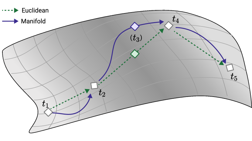
Figure 1: Depicted of difference between two sequential points in manifold space and Euclidean space. In particular, modeling and handling for the missing value $t_{3}$ require a technique that considers the characteristics of the manifold space.

TABLE I: Summary of related works categorized by space, continuous, approach.

Methods	Space	Continuous	Irregularity	Description
GRU-D [7]			$\checkmark$	GRU-based missing pattern representation learning
WEASEL+MUSE [8]	Euclidean			Similarity measure with bag-of-pattern
TapNet [9]				Distance-based low-dimensional feature representation learning
ShapeNet [10]				Shapelet-neural network
TS2Vec [11]				Hierarchical contrastive learning for a universal time-series representation
ODE-RNN [12]		$\checkmark$	$\checkmark$	Learning hidden dynamics by neural ODE
GRU-ODE [13, 14]		$\checkmark$	$\checkmark$	Neural ODE analogous to GRU
ODE2VAE [15]		$\checkmark$	$\checkmark$	Second order ODE for high-dimensional continuous data
Neural CDE [16]		$\checkmark$	$\checkmark$	Neural controlled differential equation model for irregularly-sampled data
SPDSRU [17]	Manifold			Arithmetic and geometric operations for SPD hard constraints
ManifoldDCNN [1]				Dilated CNN network for manifold-valued sequential data
MCNF [18, 19]		$\checkmark$		Neural manifold ODE for continuous normalizing flows
Ours	Manifold	$\checkmark$	$\checkmark$	Systematic integration of GRU and ODE
				with diffeomorphism mappings from SPD space to Cholesky space

While there has been a number of literature on algorithms and pattern analysis methods, deep learning has recently been most exhaustively employed as the de facto standard for time-series modeling. These approaches use convolutional neural networks (CNNs) or recurrent neural networks (RNNs) to capture spatial or temporal features of time-series data [20, 21, 22, 9, 10]. Recently, Transformer-based methods [23, 24] have been used to handle the lack of long-range dependency, which is one of the problems of RNN. However, these neural network-based methods suffer from (i) an inadequacy in handling non-Euclidean characteristics in data e.g., processing data in manifold space and (ii) insufficient data for processing complex and high-dimensional data. In this context, utilizing manifold space for modeling in deep learning for time series data offers several notable advantages compared to traditional Euclidean approaches. By effectively capturing the intrinsic non-linearity inherent in time series data and employing a mapping procedure onto lower-dimensional manifold, deep learning models become capable of adeptly capturing intricate temporal patterns and dependencies that would otherwise go unnoticed in Euclidean representations [25, 26, 27]. Consequently, this facilitates the attainment of more precise and expressive data representations. Furthermore, the adoption of manifold space learning engenders heightened robustness of models to the influences of noise and outliers [26], an augmented capacity for generalization through an emphasis on crucial variations [27], hence providing a more condensed and abstract perspective of temporal patterns. These advantages collectively contribute to advancing more dependable, efficient, and interpretable models for time series analysis.

Simultaneously, researchers have actively explored manifold space as a computational method for efficiently handling the geometric features of data. Such approaches are often used for the analysis of various representations, including but not limited to shapes [28], graphs and trees [29, 30], symmetric positive definite (SPD) matrices [31, 32], and rotation matrices [33]. Of these data types, the SPD matrix has received considerable attention in a variety of application areas due to its ability to learn suitable statistical representations [34, 35, 36]. In computer vision, SPD matrices have achieved great success as representations for classification tasks such as skeletal-based human behavioral recognition [37] and emotion recognition [34]. In signal processing, it has also been used as an expression method for multivariate time-series (MTS) data [35]. In neuroimage data analysis, a diffusion tensor image, which indicates structural connections over brain regions, has been treated as manifold-valued data [36]. Nevertheless, the direct use of SPD matrices remains a challenge because of its rigid constraints. SPD matrices in the Euclidean metric cause unfavorable results, such as the swelling effect [38] and a finite distance of symmetric matrices with non-positive eigenvalues [39, 40]. Thus, it is unreasonable for conventional deep-learning methods to model SPD matrices by ignoring their geometric characteristics and computational constraints. Additionally, backpropagation in the optimization process makes it difficult for operand components within deep neural networks to maintain positive definiteness. To address these problems, several methods have been proposed to train the model while maintaining the structure of the SPD matrix. For instance, SPDNet [34] handles this issue through an orthogonal weight matrix on the compact Stiefel manifolds. In [41], the optimizer structure was designed through a meta-learning-based method. Furthermore, existing deep learning methodologies, e.g., CNN-based models [1, 36] or RNN-based models [17], were proposed to deal with the manifold-valued sequential data, suggesting a recursive method for the weighted Fréchet mean to avoid the problems of high computational cost and instability in optimization. However, numerical errors and excessive costs remain challenges in the computation process.

Generally, modeling time-series data is based on the premise of discrete observations and emission intervals. However, data in the real world are mainly irregularly-sampled data possibly due to unexpected errors in recording or device. Fig. 1 presents an example of time-series data with one missing value at a time point $t_{3}$ on a discrete-time interval. When modeling and handling the missing value using an imputation technique, e.g., bi-linear interpolation, in a Euclidean metric (green-colored arrows), it causes a large error compared to the one estimated in a manifold metric. Even when given two data points with the same interval, its latent representations in the manifold take the form of a curve (rather than a linear form) due to the geometric characteristics. Notably, it is beneficial to model in a continuous-time space so that the geometric features inherent in the data are better represented, thus improving target downstream tasks. Therefore, it is of paramount importance to develop a continuous manifold learning method for time-series modeling.

A recent provocative approach to deal with irregularly sampled data is a continuous-time model through ordinary differential equations (ODE) with a time variable [42]. Neural ODE [42] and its variants [12, 13] have demonstrated their capability in signal representation by capturing dynamics over the internal hidden states. Subsequent studies extend the neural ODE to the manifold space [18, 19]. For example, Manifold ODE [18] has been proposed to learn the dynamics of the states in the Riemannian manifold, aiming to estimate complicated distributions in the framework of normalizing flow [43]. Although various neural ODEs for manifold space have been proposed, their application for time-series data is still limited and, even if applicable, computationally expensive and inefficient.

In this work, we propose a novel method of continuous manifold learning on sequential manifold-valued data for time-series modeling. Based on rigorous mathematical justifications, we propose to exploit a diffeomorphism mapping between Riemannian manifolds and a Cholesky space [40], by which it becomes feasible to efficiently solve optimization problems and to greatly reduce computational costs. We devise an algorithm to solve an optimization problem under the SPD constraint and achieve an effective computation cost by re-defining operations within a deep neural network framework. Our proposed method represents manifold-valued sequential data via a practical computation based on well-defined mathematical formulations. Particularly, we introduce a recurrent neural model on the Cholesky space, making it possible to greatly enhance computational efficiency and train network parameters with conventional backpropagation. Moreover, the proposed method successfully learns real-world continuous data modeling for irregularity or sparsity and adjusts the discrepancy in geodesics with the use of a manifold ODE for dynamics representation utilizing an RNN-based network. To prove the validity and robustness of our proposed method, we conducted exhaustive experiments and achieved promising performance over various public datasets.

In summary, there are three major contributions of this work:

• To handle the hard constraints of an SPD matrix in time-series modeling, we devise a novel computational mechanism that exploits a diffeomorphism mapping from SPD space to Cholesky space and applies it to a deep recurrent network. Our proposed method greatly reduces computational costs and numerical errors, thus enabling robust and stable learning.

• We also develop a manifold ODE representing temporal dynamics inherent in time-series data, allowing it to learn trajectory with geometric characteristics of sequential manifold-valued data.

• We exhaustively demonstrate the effectiveness of the proposed method through experiments over various public datasets, achieving state-of-the-art performance.

We organized the rest of this work as follows. Section 2 briefly reviews related work. In Section 3, we describe essential preliminary concepts to pave the way for understanding the proposed method. Then, Section 4 introduces the proposed method for continuous manifold learning with the diffeomorphism estimation. Section 5 describes experimental settings in detail for reproducibility and results are compared with existing methods. Finally, we conclude the study and recommend future research directions in Section 6.

TABLE II: Summary of operations in the Riemannian space and the Cholesky space. The notations used in the operations are as follows; $d$: the dimension of a matrix, $P$: a point in Riemannian space, $Q$: a point in tangent space of Riemannian space, $X,Y,L$: points in Cholesky space, $K$: a point in tangent space of Cholesky space. Note that for the distance in Riemannian space, we denote the affine-invariant Riemannian metric.

Manifold	Riemannian space	Cholesky space
	$\mathcal{S}^{+}_{d}=\{P\in\mathbb{R}^{d\times d}:P=P^{\top},\mathbf{x}^{\top}P\mathbf{x}>0,\forall\mathbf{x}\in\mathbb{R}^{d}\setminus\{\mathbf{0}_{d}\}\}$	$\mathcal{L}_{+}=\{X\in\mathbb{R}^{d\times d}:\mathcal{D}(X)>0,\{X_{ij}\}_{i>j}=0\}$
Metric	$\mathcal{T}_{X}\mathcal{M}\times\mathcal{T}_{X}\mathcal{M}$	$\sum_{i>j}X_{ij}Y_{ij}+\sum^{m}_{j=1}X_{jj}Y_{jj}L^{-2}_{jj}$
Distance	$\frac{1}{2}||\log(P_{1}^{-\frac{1}{2}}P_{2}P_{1}^{-\frac{1}{2}})||_{F}$	$\{||\lfloor L\rfloor-\lfloor K\rfloor||^{2}_{F}+||\log\mathcal{D}(L)-\log\mathcal{D}(K)||^{2}_{F}\}^{\frac{1}{2}}$
Exponential map	$P^{\frac{1}{2}}\exp(P^{\frac{1}{2}}QP^{-\frac{1}{2}})P^{\frac{1}{2}}$	$\lfloor X\rfloor+\lfloor K\rfloor+\mathcal{D}(X)\exp\{\mathcal{D}(K)\mathcal{D}(X)^{-1}\}$
Logarithmic map	$Q^{\frac{1}{2}}\log(Q^{\frac{1}{2}}PQ^{-\frac{1}{2}})Q^{\frac{1}{2}}$	$\lfloor X\rfloor-\lfloor K\rfloor+\mathcal{D}(K)\log\{\mathcal{D}(K)^{-1}\mathcal{D}(X)\}$

2 Related Work

In this section, we introduce existing research on discrete and continuous time-series modeling. TABLE I compares recent methods with our proposed in terms of computing space, continuous, and time regularity.

2.1 Discrete Time-Series Modeling

Most general models employed as baselines in time-series data are distance function-based methods [44]. Traditionally, nearest neighbor (NN) classifiers with distance functions [45] have been widely used, and the method used with Dynamic Time Warping (DTW) in particular has shown good performance [46]. In WEASEL-MUSE [8], a bag of Symbolic Fourier Approximation (SFA) is used for MTS classification. However, these classical models have limited scope and may face challenges when dealing with complex patterns, as well as limitations in terms of computational cost, sensitivity to outliers, and potential data loss.

Recently, deep learning-based methods have shown promising performance. In MLSTM-FCN [21], a model combining long short-term memory (LSTM) and CNN is proposed for MTS classification tasks. Specifically, performance is improved by adding squeeze-and-excitation blocks [47]. In [22], an unsupervised method is proposed to solve the variable lengths and sparse labeling problems of time-series data. The authors process the variable length through a dilated convolutional [48] encoder and build a triplet loss [49] with negative samples. Meanwhile, for high-dimensional multivariate data and limited training label problems, TapNet [9] proposes an attentional prototype network by learning low-dimensional features through random group permutation. In ShapeNet [10], the author proposes an MDC-CNN with a triplet loss that trains time-series subsequences of various lengths in a unified space. Meanwhile, transformer-based methods [23, 24] have been mainly used for forecasting time-series data, especially due to their ability to model long-range dependencies. Representation learning for time series data has garnered significant attention in recent years. Of various techniques, contrastive learning-based methods have emerged as prominent approaches, offering universal representation learning for various time series data tasks [11, 24]. Zerveas et al. [24] propose an unsupervised representation learning method based on transformers, evaluating its effectiveness in multivariate time series regression and classification. In [11], TS2Vec is introduced as a technique for learning universal representations at different semantic levels. Although these models use deep learning-based methods to learn spatio-spectral-temporal features from time-series data, they are limited in the assumption that the data have constant intervals and thus are most suitable for regular time-series data. In contrast, our proposed method is a neural ODE-based method that enables continuous time-series modeling.

2.2 Continuous Modeling

Meanwhile, researchers have focused on modeling dynamic patterns at continuous time points. Foremost, [42] proposes the idea of parameterizing derivatives of hidden states for continuous modeling. Inspired by neural ODEs, [12] propose latent ODE and ODE-RNN to deal with irregularly-sampled data. In [13], GRU-ODE-Bayes, combining GRU-ODE and GRU-Bayes, is proposed to address sporadic observations that occur in multidimensional time-series data. Theoretically similar to [13], in Neural CDE [16], an extended model of Neural ODE using a controlled differential equation is proposed to address the limitations of an ordinary differential equation. Meanwhile, in ODE2VAE, by decomposing the latent space into position and velocity components, time-sequential modeling for sequential data is proposed [15]. In [50], for the relevance or importance of individual samples, a continuous-time attention method is proposed by applying the attention mechanism to the neural ODE.

Recent studies on the use of neural ODEs have begun to model structured [51] or manifold-valued data [18]. To capture the essence of continuous node representations, [51] introduces a graph-based model. Within the research community, neural ODEs have been expanded from their original domain of Euclidean space to encompass a manifold space, particularly in normalizing flow tasks [18, 19]. Even with the potential demonstrated by these advancements, a substantial gap exists in research regarding applying neural ODEs to high-dimensional time-series data. In contrast, our model takes a different approach by employing neural ODEs to specifically address continuous time-series modeling, focusing on the trajectories of hidden states within a manifold space while incorporating structural features.

2.3 Manifold Learning

In order to better represent the geometric characteristics inherent in time-series data, recent studies focus on modeling with manifold-valued data, especially SPD matrices, in deep learning frameworks. In [34], the author proposes an SPDNet that consists of fully connected convolution-like layers, rectified linear units-like layers, and eigenvalue logarithm layers to train the deep model while maintaining the data structure on the SPD matrix. Subsequently, [52] redefines the batch normalization on SPDNet using Riemannian operations to improve the classification performance and robustness of the model. In [35], the author proposes a metric learning-based SPD model that divides the classification problem into sub-problems and builds a single model to solve each sub-problem. Succinctly, SPDNet models are presented based on mapping with sub-manifold, but the repeated eigenvalue decomposition in the process inevitably generates tremendous computation costs.

Meanwhile, [17] proposes a deep model based on statistical machine learning when data are ordered, longitudinal, or temporal in a Riemannian manifold. Additionally, to resolve the slow speed issue of RNN-based models, the dilated and causal CNNs were defined in the manifold space [36, 1]. In [53], a flow-based generative model for manifold-valued data is introduced through three types of invertible layers in a generative regime. Training a deep model while maintaining the SPD constraint is challenging due to huge computational costs and unstable training.

Our approach differs from these previous SPD manifold methods, which directly process the SPD matrix. We accomplished this through mapping into the Cholesky space, which is easy to compute. This way, our proposed method relaxes the constraints enough to allow the optimization to be processed with the training algorithms.

3 Preliminaries

In this section, we concisely provide useful definitions and operations for Riemannian geometry. The notations and operations in Riemannian and Cholesky spaces are summarized in TABLE II. Note that our development is based on the diffeomorphism mapping of Cholesky decomposition, thus in Riemannian Cholesky space rather than in the Riemannian geometry of SPD matrices. In the following, $\lfloor\cdot\rfloor$ and $\mathcal{D}(\cdot)$ denote the strictly lower triangular and the diagonal part of a matrix, respectively.

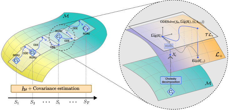
Figure 2: For the overall framework of the proposed method, first, input sequences $\{S_{i}\}_{1,\cdots,T}$ are fed into a feature extraction network $h_{\theta}$ for high-level representation. The manifold point $\{C_{i}\}_{1,\cdots,T}$ obtained by covariance estimation is then decomposed to $\{X_{i}\}_{1,\cdots,T}$ in the Cholesky space. Our proposed Riemannian manifold gated recurrent unit (RGRU) calculates Cholesky points, then the estimated points are mapped into the tangent space of the ordinary differential equation (ODE) solver ($\operatorname{ODESolve}$) through a logarithmic map $\widetilde{\operatorname{Log}}(\cdot)$. Afterward, the output of the ODE solver at the $i$-th timepoint $H^{\prime}_{i}$ is projected to Cholesky space $\mathcal{L}_{+}$ by an exponential map $\widetilde{\operatorname{Exp}}(\cdot)$.

3.1 Riemannian Manifold and Metric on Cholesky Space [40].

A Riemannian manifold $(\mathcal{M},g)$ is a real, smooth manifold $\mathcal{M}$ equipped with a positive-definite inner product $g_{X}$ on the tangent space $\mathcal{T}_{X}\mathcal{M}$ at each point $X\in\mathcal{M}$. The $g_{X}$ is called a Riemannian metric, making it possible to define several geometric notions on a Riemannian manifold, such as the angle and curve length.

The space $\mathcal{S}^{+}_{d}$ of $d\times d$ SPD matrices is a smooth submanifold of the space $\mathcal{S}_{d}$ of symmetric matrices, whose tangent space at a given SPD matrix is identified with $\mathcal{S}_{d}$. Cholesky decomposition represents a matrix $S\in\mathcal{S}^{+}_{d}$ as a product of a lower triangular matrix $L$ and its transpose, i.e., $S=LL^{\top}$. The smooth submanifold $\mathcal{L}_{+}$ of the space of lower triangular matrices $\mathcal{L}$ with diagonal elements all positive defines a Cholesky space. Note that the tangent space of $\mathcal{L}_{+}$ at a given matrix $L\in\mathcal{L}_{+}$ is identified with the linear space $\mathcal{L}$. Let the strict lower triangular space $\lfloor\mathcal{L}\rfloor=\{\lfloor X\rfloor|X\in\mathcal{L}\}\in\mathbb{R}^{d(d-1)/2}$ with the Frobenius inner product $\langle X,Y\rangle_{F}=\sum^{d}_{i,j=1}X_{ij}Y_{ij}$, $\forall$ $X,Y\in\lfloor\mathcal{L}\rfloor$, while denoting the diagonal part $\mathcal{D}(\mathcal{L})=\{\mathcal{D}(X)|X\in\mathcal{L}\}$ with a different inner product $\langle\mathcal{D}(L)^{-1}\mathcal{D}(X),\mathcal{D}(L)^{-1}\mathcal{D}(Y)\rangle_{F}$. Then, we define a metric $\tilde{g}$ for the tangent space $\mathcal{T}_{L}\mathcal{L}_{+}$ as follows,

$$\tilde{g}_{L}(X,Y) =\langle X,Y\rangle_{F}+\langle\mathcal{D}(L)^{-1}\mathcal{D}(X),\mathcal{D}(L)^{-1}\mathcal{D}(Y)\rangle_{F}$$

$$=\sum^{d}_{i=1}\sum^{i}_{j=1}X_{ij}Y_{ij}+\sum^{d}_{j=1}X_{jj}Y_{jj}L^{-2}_{jj}.$$ (1)

Proposition 1. [40] Cholesky map $\mathfrak{L}$ is a diffeomorphism between smooth manifolds $\mathcal{L}_{+}$ and $\mathcal{S}^{+}_{d}$.

The full proof of Proposition 1 can be found in [40]. Essentially, the Cholesky map easily represents deep learning processes in the SPD manifold space.

3.2 Exponential and Logarithmic Maps

For any $P\in\mathcal{S}^{+}_{d}$ and $Q\in\mathcal{S}_{d}$, the exponential map $\operatorname{Exp}_{P}:\mathcal{S}_{d}\rightarrow\mathcal{S}^{+}_{d}$ and the logarithmic map $\operatorname{Log}_{Q}:\mathcal{S}^{+}_{d}\rightarrow\mathcal{S}_{d}$ are defined as

$$\operatorname{Exp}_{P}(Q) =P^{\frac{1}{2}}\exp(P^{\frac{1}{2}}QP^{-\frac{1}{2}})P^{\frac{1}{2}}\in S^{+}_{d},$$ (2)

$$\operatorname{Log}_{Q}(P) =Q^{\frac{1}{2}}\log(Q^{\frac{1}{2}}PQ^{-\frac{1}{2}})Q^{\frac{1}{2}}\in S_{d}.$$ (3)

Generally, it is difficult to compute Riemannian exponential and logarithmic maps because they require evaluating a series of infinite number of terms [39]. However, by mapping to Cholesky space, we obtain easy-to-compute expressions for Riemannian exponential and logarithmic maps. Let $X\in\mathcal{L}_{+}$ and $K\in\mathcal{L}$. Then, we define the exponential map $\widetilde{\operatorname{Exp}}$ and the logarithmic map $\widetilde{\operatorname{Log}}$ as in [40]

$$\widetilde{\operatorname{Exp}}_{X}(K) =\lfloor X\rfloor+\lfloor K\rfloor+\mathcal{D}(X)\exp\{\mathcal{D}(K)\mathcal{D}(X)^{-1}\},$$ (4)

$$\widetilde{\operatorname{Log}}_{K}(X) =\lfloor X\rfloor-\lfloor K\rfloor+\mathcal{D}(K)\log\{\mathcal{D}(K)^{-1}\mathcal{D}(X)\}.$$ (5)

For the convenience of expression, we omit the subscript (i.e., $\widetilde{\operatorname{Exp}}_{X}=\widetilde{\operatorname{Exp}}$)

3.3 Fréchet Mean

The Fréchet mean [54] is an extension of the Euclidean mean, widely used to aggregate representations in neural networks such as attention [4] and batch normalization [55], showing strong theoretical and practical interest in Riemannian data analysis. Given $\{P_{i}\}_{i=1}^{N}$ samples on $\mathcal{S}^{+}_{d}$, the Fréchet mean is defined as

$$\mu=arg\min_{G\in\mathcal{S}^{+}_{d}}\sum^{N}_{i=1}\delta_{R}^{2}(G,P_{i}).$$ (6)

where $\delta_{R}$ is the Riemannian distance between two points on the manifold. Unfortunately, the solution to the minimization problem in Eq. (6) is unknown in closed-form, but is usually computed using an iterative solver, e.g., Karcher flow [56], that approximates the solution by computing in tangent space and mapping back to manifold space via logarithmic and exponential maps, respectively. However, the Fréchet mean in Cholesky space is closed and easy to compute. That is, an iterative operation is not required. We call this the log-Cholesky mean $\mu_{\mathcal{L}_{+}}$ and it is defined as [40]

$$\mu_{\mathcal{L}_{+}}=\frac{1}{N}\sum^{N}_{i=1}\lfloor X_{i}\rfloor+\exp\Big{\{}N^{-1}\sum^{N}_{i=1}\log\mathcal{D}(X_{i})\Big{\}}.$$ (7)

3.4 Manifold ODE

We introduce the ordinary differential equations in manifold space. Suppose that $\mathbf{z}(t)$ is a differentiable curve with values in $\mathcal{M}$. Then, by the definition of the tangent space, its derivative $d\mathbf{z}(t)/dt\in\mathcal{T}_{\mathbf{z}(t)}\mathcal{M}\;\forall t$. This assumption leads to the following definition:

Definition 1. Let $\mathcal{M}$ be a manifold space. A vector field $f$ in regard to the dynamics is a $\mathcal{C}^{1}$-mapping such that

$$\frac{d\mathbf{z}(t)}{dt}=f(\mathbf{z}(t),t)\in\mathcal{T}_{\mathbf{z}(t)}\mathcal{M}.$$ (8)

A vector field $f$ is called a differential equation on the manifold, and a function $z$ is called an integral curve or simply a solution of the equation.

According to Definition 1, a vector field is defined at arbitrary intervals in the manifold space. We consider the interval $[t_{1},t_{2}]$ such that $z_{1}=\mathbf{z}(t_{1})$. Since the solution of a differential equation depends on the initial point, we obtain the notation $\varphi_{t_{2}}(z_{1})=\mathbf{z}(t_{2})$ for the solution at time $t_{2}$ with an initial condition $z_{1}=\mathbf{z}(t_{1})$.

4 Continuous Manifold Learning on Riemannian Cholesky Space

This section introduces our proposed method of continuous manifold learning in Cholesky space from sequential manifold-valued data for time-series modeling. We illustrate the overall procedures in Fig. 2.

4.1 Mapping to the Riemannian Cholesky Space

For manifold learning, we first transform the input time-series data into manifold space. Specifically, we exploit second-order statistics (i.e., covariance) of features represented via a function $h_{\theta}$, then use a shrinkage estimator [57], to estimate second-order statistics and thus, represent an SPD matrix in manifold space. Then, an SPD matrix $S$ is decomposed into a lower triangular matrix $X$ and its transpose $X^{\top}$ by Cholesky decomposition $C(S)=XX^{\top}$. We express the lower triangular matrix $X$ as the sum of the strictly lower part and the diagonal part as $X=\lfloor X\rfloor+\mathcal{D}(X)$.

Generally, it is challenging to train a network in SPD Riemannian manifold due to: (1) there are mathematical constraints in optimization, e.g., the convexity of weights in FM estimation [17], the validity of the output to be an SPD matrix [34], and (2) numerical errors that occur by distorting the geometric structure during the learning process, especially when the dimension of a matrix increases [58]. Meanwhile, when conducting operations in Cholesky space, due to the nice properties of the Cholesky matrices, we only consider the constraint that the elements of the diagonal matrix $\mathcal{D}(X)$ should be positive, and the elements in $\lfloor X\rfloor$ are unconstrained. Thus, by taking advantage of operating in the Cholesky space, it becomes relatively easier to solve an optimization problem.

4.2 Recurrent Network Model in Cholesky Space

An RNN equipped with gated recurrent units (GRU) [59] is successfully used for time-series modeling in various applications. Here, we introduce a novel Riemannian manifold GRU (RGRU) by reformulating gating operations in the Cholesky space. It is worth noting that the reformulated operations apply not only to GRU but also to LSTM. Compared with existing deep learning methods for SPD matrix modeling [17, 53, 1, 36, 34, 52, 41, 35], as we formulate the optimization problem in a Cholesky space with a unique constraint of positivity in values of the diagonal part of $\mathcal{D}(X)$, the optimization is solved relatively easily and with efficient computations, thus making their computation costs cheap.

Let us reformulate the gating operations and feature representations in terms of the Cholesky geometry with (i) weighted Fréchet mean (wFM), (ii) bias addition, and (iii) non-linearity. First, the wFM is defined using Eq. (7) for the weighted combination of Cholesky matrices as follows

$$\operatorname{wFM}( \left\{X_{i}\right\}_{i=1,\cdots,N},\mathbf{w}\in\mathbb{R}^{N}_{\geq 0})$$

$$= \frac{1}{N}\sum^{N}_{i=1}(w_{i}\cdot\lfloor X_{i}\rfloor)+\exp\Big{\{}N^{-1}\sum^{N}_{i=1}w_{i}\cdot\log\mathcal{D}(X_{i})\Big{\}}$$ (9)

where $\mathbb{R}_{\geq 0}$ denotes a space of non-negative real numbers and $w_{i}$ denotes the $i$-th element of the weight vector $\mathbf{w}$. Second, for the bias addition, we define an operator $\oplus$ on $\mathcal{L}_{+}$ [40] by

$$X\oplus Y=\lfloor X\rfloor+\lfloor Y\rfloor+\mathcal{D}(X)\mathcal{D}(Y).$$ (10)

Such an operation $\oplus$ is a smooth commutative group operation on the manifold $\mathcal{L}_{+}$. Since this group operation is a bi-invariant metric, we regard the operation for translation, analogous to the case in Euclidean space. Third, regarding the non-linearity, since the off-diagonal values are unconstrained but the diagonal values should be positive, we handle elements of the off-diagonal and the diagonal parts separately by applying two independent activation functions accordingly and then adding the resulting values to obtain a valid Cholesky matrix, e.g., $\text{tanh}(\lfloor X\rfloor)+\text{softplus}(\mathcal{D}(X))$.

Given a sequence of SPD matrices $\mathbf{X}=\{X_{1},X_{2},\cdots,X_{T}\}$ on $\mathcal{L}_{+}$ obtained from an input time-series sample by passing through the feature extractor $H_{\theta}$ and the covariance estimation module consecutively, we reformulate the gating and representation operations involved in our RGRU as follows

$$\left\{\begin{array}[]{c l}\mathbf{z}_{i}&=\sigma(\text{wFM}(\left\{X_{i},H_{i-1}\right\},W_{z})\oplus B_{z}),\\ \mathbf{r}_{i}&=\sigma(\text{wFM}(\left\{X_{i},H_{i-1}\right\},W_{r})\oplus B_{r}),\\ \mathbf{l}_{i}&=\text{wFM}(\left\{X_{i},\mathbf{r}_{i}\odot H_{i-1}\right\},W_{l})\oplus B_{l},\\ \hat{H}_{i}&=\text{tanh}(\lfloor\mathbf{l}_{i}\rfloor)+\text{softplus}(\mathcal{D}(\mathbf{l}_{i})),\\ H_{i}&=(1-\mathbf{z}_{i})\odot H_{i-1}+\mathbf{z}_{i}\odot\hat{H}_{i},\end{array}\right.$$ (16)

where $H_{i}\in\mathcal{L}_{+}$ is the hidden state in RGRU, $\mathbf{z}_{i}\in\mathcal{L}_{+},\mathbf{r}_{i}\in\mathcal{L}_{+}$ and $\hat{H}_{i}\in\mathcal{L}_{+}$ are the update gate, the reset gate, and candidate hidden state, respectively; $\{W_{z}\in\mathcal{L}_{+},W_{r}\in\mathcal{L}_{+},W_{l}\in\mathcal{L}_{+}\}$ are learnable weights and $\{B_{z}\in\mathcal{L}_{+},B_{r}\in\mathcal{L}_{+}$, $B_{l}\in\mathcal{L}_{+}\}$ are corresponding learnable biases; $\sigma(\cdot)$ is a logistic sigmoid function, tanh($\cdot$) is a hyperbolic tangent function, and softplus$(\cdot)$ is a softplus function, and $\odot$ denotes an operator of element-wise multiplication that satisfies the group axiom. It is worth noting that without loss of generality, any activation function with a positive output range, e.g., sigmoid, can be used in the position of a softplus function.

4.3 Neural Manifold ODE

For continuous manifold learning, we further leverage the technique of neural manifold ODEs [18] in sequential data modeling and model the dynamics of $f$ by a neural network with its learnable parameters $\Theta$. Here, we define both the forward and backward pass gradient computations for network parameter learning. Notably, the forward pass is computed in manifold space but the backward pass is defined solely through an ODE in Euclidean space.

4.3.1 Forward Mode

Forward mode integration is broadly classified into two groups: a projection method [60] and an implicit method [18, 60, 61]. In this work, we employ an implicit method due to its general applicability in any manifold space and its definition using step-based solvers [62, 61]. Particularly, we use a variant of an Euler method solver with an update step $h_{t+\epsilon}=\exp_{H_{t}}(\epsilon f_{\Theta}(H_{t},t))$ for the Riemannian exponential map [62]. Here, $\epsilon$ is a time step.

4.3.2 Backward Mode

Recently, [42] and [18] proposed an adjoint sensitivity method to effectively compute the gradients and calculate the derivative of a manifold ODE, independently. In our method, we use the adjoint method to compute the derivative of a manifold ODE.

In differential geometry, $D_{x}f_{\Theta}:\mathcal{T}_{x}\mathcal{M}\rightarrow\mathcal{T}_{x}\mathcal{N}$ defines a derivative of a function $f_{\Theta}:\mathcal{M}\rightarrow\mathcal{N}$ mapping between two manifolds.

Theorem 1. [18] We define a loss function $E:\mathcal{M}\rightarrow\mathbb{R}$. Suppose that there is an embedding of manifold space $\mathcal{M}$ in Euclidean space $\mathbb{R}^{d}$. Let the adjoint state be $\mathbf{a}(t)=D_{\mathbf{z}(t)}E$, then the adjoint satisfies

$$\frac{d\mathbf{a}(t)}{dt}=-\mathbf{a}(t)D_{\mathbf{z}}(t)f_{\Theta}(\mathbf{z}(t),t)$$ (17)

In the implementation, we construct the differential equation

$$\frac{d\widetilde{\operatorname{Log}}(H_{t})}{dt}=D_{\widetilde{\operatorname{Exp}}(H_{t})}\widetilde{\operatorname{Log}}\Big{(}f_{\Theta}(\widetilde{\operatorname{Exp}}(H_{t}),t)\Big{)}$$ (18)

Then, $\widetilde{\operatorname{Log}}(H_{t})$ is solved using the numerical integration technique. Finally, we can update $H_{t}$ to $H_{t+\epsilon}$. With the adjoint state, we calculate the gradients with respect to the start and end time points, $t_{s}$, $t_{e}$ with the initial condition $H_{s}$, and the weights $\Theta$.

Input : Time-series data $\mathbf{S}=\{S_{i}\}_{i=1,\ldots,T}$ and time stamps $\mathbf{t}=\{t_{i}\}_{i=1,\ldots,T}$, learnable model parameters $\theta,\;\Theta$

Output : $\{H_{i}\}_{i=1,\cdots,T}$

1:  $\{S^{\prime}_{i}\}_{i=1,\ldots,T}=h_{\theta}(\mathbf{S})$

12:  $\{C^{\prime}_{i}\in\mathcal{S}^{+}_{d}\}_{i=1,\ldots,T}=\operatorname{SE}(\{S^{\prime}_{i}\}_{i=1,\ldots,T})$  // SE: Shrinkage Estimation

23:  $\{X_{i}X_{i}^{\top}\}_{i=1,\ldots,T}=\operatorname{CD}(\{C^{\prime}_{i}\}_{i=1,\ldots,T})$  // CD: Cholesky Decomposition

34:  $H_{0}=\mathbf{I}$  // Identity matrix

5:  for $i$ in $1,2,\cdots,T$ do

6:     $H^{\prime}_{i}=$ ODESolve$(f_{\Theta},\widetilde{\operatorname{Log}}(H_{i-1}),(t_{i-1},t_{i}))$

47:     $H_{i}=$ RGRU$(\widetilde{\operatorname{Exp}}(H^{\prime}_{i}),X_{i})$  // Eq. (16)

8:  end for

9:  return $\{H_{i}\}_{i=1,\cdots,T}$

Algorithm 1 Pseudo algorithm of ODE-RGRU

4.4 ODE-RGRU

Here, we describe the systematic integration of manifold ODE and RGRU in a unified framework for sequential continuous manifold modeling, called ODE-RGRU. Formally, the ODE-RGRU is formulated as

$$H^{\prime}_{i} =\text{ODESolve}(f_{\Theta},\widetilde{\operatorname{Log}}(H_{i-1}),(t_{i-1},t_{i}))$$ (19)

$$H_{i} =\text{RGRU}(\widetilde{\operatorname{Exp}}(H^{\prime}_{i}),X_{i}),$$ (20)

where $X_{i}\in\mathcal{L}_{+}$ is an input manifold-valued feature and $H_{i}$ is a latent state at the $i-$th timepoint, for $i=1,\cdots,T$. We define such a hidden state $H^{\prime}_{i}$ to be the solution on tangent space after mapping via $\widetilde{\operatorname{Log}}$ to an ODESolver and then the output of the ODESolver is orthogonally projected to a manifold space by an exponential map $\widetilde{\operatorname{Exp}}$. The initial hidden state $H_{0}$ is set to identity matrices $\mathbf{I}$ that satisfy the SPD constraint. For each observation over time, the corresponding hidden state is updated in the Cholesky space using Eq. (16), i.e., RGRU. The overall algorithm of ODE-RGRU is summarized in Algorithm 1. Note that Algorithm 1 focused on the representation of the hidden state, while the proposed model concentrated on mapping to the Cholesky space within the SPD matrix. However, considering the diffeomorphic properties between these two spaces, it is also possible to apply a mapping from the Cholesky space to the SPD space. Thus, depending on the desired objective, mapping between the Cholesky space and the SPD space is feasible, offering flexibility in achieving the intended goals.

4.5 Computational Time Efficiency

It should be noted that the computation of manifold space point representations in our proposed model relies on CPU-based operations, which may result in slower training times compared to conventional time series modeling approaches. However, this limitation is mitigated by the inherent statistical characteristics of data and the model’s capacity for effective generalization. Consequently, despite the potential trade-off in computational speed, the model enables efficient optimization and exhibits rapid convergence due to its ability to leverage the intrinsic statistical properties of data [63].

To learn geometric information in a neural network through manifold learning, the internal operations should consider and satisfy manifold constraints. Specifically, the SPD matrix appears in various domains, but it is difficult to train a neural network because of rigid constraints, i.e., symmetries and all positive eigenvalues. To tackle such challenges, [34] train their model in a compact Stiefel manifold space and [41] applied Euclidean operations in a tangent space with a logarithmic map and switched to manifold space with an exponential map. Most operations are performed through the Eigenvalue decomposition with a computational complexity of $O(k\cdot n^{3})$ on $k$ iterations for Fréchet mean estimation. That is, as the dimensions of the matrices of interest increase, the computational cost increases exponentially. Therefore, the previous work [64] derives explicit gradient expressions so that manifold learning could be performed in a reasonable computational time, but it was limited to hyperbolic space. Consequently, it remains that a computational problem exists in the Riemannian manifold for the Fréchet mean estimation, thus making the model’s training slow and unstable.

In this work, we propose to exploit the Cholesky decomposition, which finds a unique lower triangular matrix for an SPD matrix. The nice properties of a Cholesky matrix allow efficient numerical calculations. Moreover, it has simple and easy-to-compute expressions for Riemannian exponential and logarithmic maps. Notably, it provides a closed-form solution for the weighted Fréchet mean with a linear computational complexity.

5 Experiments

In this section, we evaluate the proposed method for real-world applications of video action recognition, sleep staging classification, and various multivariate time-series modeling tasks by using publicly available datasets. Our implementation code used for the experiments is available at ”https://github.com/ku-milab/Deep-Efficient-Continuous-Manifold-Learning” and all the implementation details are provided in our GitHub repository.

TABLE III: Performance (mean$\pm$std, %) on an action recognition task (UCF11).

Method	# Parameters	Accuracy
ODE-RGRU (Ours)	66,767	89.4 $\pm$ 1.2
ManifoldDCNN [1]	3,658	82.3 $\pm$ 1.8
SPDSRU [17]	3,445	78.4 $\pm$ 1.4
TT-GRU [20]	202,667	81.3 $\pm$ 1.1
TT-LSTM [20]	6,176	79.6 $\pm$ 3.5
GRU	18,602,606	79.3 $\pm$ 3.8
LSTM	24,791,606	71.4 $\pm$ 2.7

5.1 Datasets and Preprocessing

5.1.1 Action Recognition

For the action recognition task, we used the UCF11 [65] dataset. The UCF11 dataset is composed of 1,600 video clips, with 11 action categories, e.g., basketball shooting, biking/cycling, diving, golf swinging, etc. The length of the video frames varies from 204 to 1492 per clip with a resolution of each frame being $320\times 240$. Similar to previous work [1, 17], we downsized all frames to $160\times 120$ and sampled 50 frames from each clip, i.e., $N=50$, with an equal time gap between frames. Then, we performed the $5$-fold cross-validation for fair evaluation, while keeping the class balance.

5.1.2 Sleep Staging Classification

We used the SleepEDF-20 [66] dataset for the sleep staging classification task. The SleepEDF-20 is the Sleep Cassette that comprises 20 subjects (10 males and 10 females) aged 25-34. Two polysomnographies were recorded during day-night periods, except for subject 13 who lost the second night due to a device problem. All signals were segmented into lengths of 30 seconds and manually labeled into 8 categories, ‘wake,’ ‘rapid eye movement (REM),’ ‘non REM1/2/3/4,’ ‘movement,’ and ‘unknown,’ by sleep experts [67]. In this work, similar to the previous studies [68, 69, 70, 5], we merged ‘non REM3’ and ‘non REM4’ stages into a ‘non REM3’ stage and removed samples labeled as ‘movement’ and ‘unknown.’ Here, we used spectrogram data rather than raw signals [71]. To achieve this, we sampled all signals at 100Hz rate and applied short-time Fourier transformation to compute spectrograms. For this experiment, we used single-channel EEG and 2-channel EEG/EOG samples. Note that we did not exploit electromyogram recordings due to their incompleteness. As a result, we obtained a multi-channel signal $S\in\mathbb{R}^{F\times T\times C}$ where $F$, $T$, and $C$ denote the number of frequency bins, the number of spectral columns, and the number of channels, respectively. We set $F=129$, $T=29$, $C=1$ or $C=2$ (for the single-channel EEG or two-channel EEG/EOG). For the staging classification, $10$ continuous segments of data were used as input, i.e., $N=10$. For a fair evaluation, we conducted a $20$-fold cross-validation by maintaining a class balance similar to [68, 69, 70, 5].

5.1.3 Multivariate Time Series Classification

To evaluate various sensor data in the classification task not only for sleep staging classification, we used the UEA archive [44], a well-known multivariate time-series data. The UEA archive consists of 30 real-world multivariate time-series data for various classification applications, e.g., Human Action Recognition, Motion classification, etc. The dimension of the archive range from 2 dimensions in AtrialFibrillation to 1345 in DuckDuckGeese, and the time length is from 8 in PenDigits to 17984 in EigenWorms. The dataset is divided into train and test sets with the train size ranging from 12 to 30000. Detailed information about each dataset can be found in [44].

5.1.4 Time Series Forecasting & Imputation

For the forecasting task, we used four public datasets, including three ETT datasets [23] and the Electricity dataset [72]. The ETT is the dataset that collects electricity transformer temperature, which is an important indicator in power long-term deployment. The ETT dataset consists of ETTh₁, ETTh₂ at a 1-hour level and ETTm₁ at a 15-minute level, and each point is expressed as an oil temperature and 6 power load features. Electricity dataset is the measurement of electric power consumption that contains 2,075,259 measurements.

For the imputation task, we collected data from the TADPOLE database, which is based on the Alzheimer’s Disease Neuroimaging Initiative (ADNI) cohort. This dataset comprises information from 1,737 patients and encompasses 1,500 biomarkers obtained over 12,741 visits spanning 22 time periods. Although the TADPOLE database offers numerous biomarkers for predicting the Alzheimer’s disease (AD) spectrum, our study focused on six volumetric MRI features, T1-weighted MRI scans, and cognitive test scores, such as the mini-mental state exam (MMSE), Alzheimer’s disease assessment scale (ADAS)-cog11, and ADAS-cog13.

TABLE IV: Performance on sleep staging classification task (SleepEDF-20). We computed accuracy (Acc), Cohen’s kappa value ($\kappa$), macro F1-score (MF1), averaged sensitivity (Sen), and averaged specificity (Spec).

Method	EEG					EEG/EOG
	Acc	$\kappa$	MF1	Sen	Spec	Acc	$\kappa$	MF1	Sen	Spec
ODE-RGRU (Ours)	86.3	0.807	80.2	80.6	96.3	86.6	0.812	80.3	81.4	96.4
ODE-RGRU (w/o ODEFunc.) (Ours)	84.1	0.774	74	75	95.6	84.3	0.777	74.8	75.7	95.7
XSleepNet [5]	86.3	0.813	80.6	80.2	96.4	86.4	0.813	80.9	79.9	96.2
SeqSleepNet [71]	85.2	0.798	78.4	78.0	96.1	86.0	0.809	79.7	79.2	96.2
FCNN + RNN [5]	81.8	0.754	75.6	75.7	95.3	83.5	0.775	77.7	77.2	95.5
DeepSleepNet [70]	-	-	-	-	-	82.0	0.760	76.9	-	-
U-time [73]	-	-	79.0	-	-	-	-	-	-	-
IITNet [74]	83.9	0.780	77.6	-	-	-	-	-	-	-

TABLE V: Performance on UEA archive. We compute the accuracy of all comparison methods, total best accuracy, average rank, and Wilcoxon-signed rank test.

Dataset	EDI	DTWI	DTWD	MLSTM	WEASEL	NS	TapNet	ShapeNet	TST	TS2Vec	ODE-RGRU
	[44]	[44]	[44]	-FCNs [21]	+MUSE [8]	[22]	[9]	[10]	[24]	[11]	(Ours)
ArticularyWordRecognition	0.970	0.980	0.987	0.973	0.990	0.987	0.987	0.987	0.977	0.987	0.973
AtrialFibrillation	0.267	0.267	0.220	0.267	0.333	0.133	0.333	0.400	0.067	0.200	0.333
BasicMotions	0.676	1.000	0.975	0.950	1.000	1.000	1.000	1.000	0.975	0.975	1.000
CharacterTrajectories	0.964	0.969	0.989	0.985	0.990	0.994	0.997	0.980	0.975	0.995	0.991
Cricket	0.944	0.986	1.000	0.917	1.000	0.986	0.958	0.986	1.000	0.972	0.986
DuckDuckGeese	0.275	0.550	0.600	0.675	0.575	0.675	0.575	0.725	0.620	0.680	0.700
EigenWorms	0.549	-	0.618	0.504	0.890	0.878	0.489	0.878	0.748	0.847	0.847
Epilepsy	0.666	0.978	0.964	0.761	1.000	0.957	0.971	0.987	0.949	0.964	0.964
ERing	0.133	0.133	0.133	0.133	0.133	0.133	0.133	0.133	0.874	0.874	0.748
EthanolConcentration	0.293	0.304	0.323	0.373	0.430	0.236	0.323	0.312	0.262	0.308	0.373
FaceDetection	0.519	-	0.529	0.545	0.545	0.528	0.556	0.602	0.534	0.501	0.620
FingerMovements	0.550	0.520	0.530	0.580	0.490	0.540	0.530	0.580	0.560	0.480	0.600
HandMovementDirection	0.278	0.306	0.231	0.365	0.365	0.270	0.378	0.338	0.243	0.338	0.311
Handwriting	0.200	0.316	0.286	0.286	0.605	0.533	0.357	0.451	0.225	0.515	0.457
Heartbeat	0.619	0.658	0.717	0.663	0.727	0.737	0.751	0.756	0.746	0.683	0.751
InsectWingbeat	0.128	-	-	0.167	-	0.160	0.208	0.250	0.105	0.466	0.548
JapaneseVowels	0.924	0.959	0.949	0.976	0.973	0.989	0.965	0.984	0.978	0.984	0.992
Libras	0.833	0.894	0.870	0.856	0.878	0.867	0.850	0.856	0.656	0.867	0.861
LSST	0.456	0.575	0.551	0.373	0.590	0.558	0.568	0.590	0.408	0.537	0.595
MotorImagery	0.510	-	0.500	0.510	0.500	0.540	0.590	0.610	0.500	0.510	0.630
NATOPS	0.850	0.850	0.883	0.889	0.870	0.944	0.939	0.883	0.850	0.928	0.950
PEMS-SF	0.705	0.734	0.711	0.699	-	0.688	0.751	0.751	0.740	0.682	0.763
PenDigits	0.973	0.939	0.977	0.978	0.948	0.983	0.980	0.977	0.560	0.989	0.986
Phoneme	0.104	0.151	0.151	0.110	0.190	0.246	0.175	0.298	0.085	0.233	0.302
RacketSports	0.868	0.842	0.803	0.803	0.934	0.862	0.868	0.882	0.809	0.855	0.868
SelfRegulationSCP1	0.771	0.765	0.775	0.874	0.710	0.846	0.652	0.782	0.754	0.812	0.823
SelfRegulationSCP2	0.483	0.533	0.539	0.472	0.460	0.556	0.550	0.578	0.550	0.578	0.550
SpokenArabicDigits	0.967	0.959	0.963	0.990	0.982	0.956	0.983	0.975	0.923	0.988	0.977
StandWalkJump	0.200	0.333	0.200	0.067	0.333	0.400	0.400	0.533	0.267	0.467	0.400
UWaveGestureLibrary	0.881	0.868	0.903	0.891	0.916	0.884	0.894	0.906	0.575	0.906	0.834
Total Best acc	0	2	1	2	9	1	3	6	2	3	10
Average Rank	6.8	6.0	5.4	5.2	4.2	4.2	4.0	2.9	6.2	3.9	2.6
Wilcoxon Test p-value	0.000	0.000	0.000	0.000	0.155	0.013	0.003	0.802	0.000	0.094	-

TABLE VI: Performance on irregular CharacterTrajectories. We computed the mean and variance of accuracy on five repeats.

Method	Test Accuracy
	30% dropped	50% dropped	70% dropped
ODE-RGRU (Ours)	98.9 $\pm$ 0.2	98.3 $\pm$ 0.2	98.6 $\pm$ 0.3
Neural CDE [16]	98.7 $\pm$ 0.8	98.8 $\pm$ 0.2	98.6 $\pm$ 0.4
ODE-RNN [12]	95.4 $\pm$ 0.6	96 $\pm$ 0.3	95.3 $\pm$ 0.6
GRU-D [7]	94.2 $\pm$ 2.1	90.2 $\pm$ 4.8	91.9 $\pm$ 1.7
GRU-$\Delta$t [16]	93.6 $\pm$ 2	91.3 $\pm$ 2.1	90.4 $\pm$ 0.8

5.2 Experimental Setting

5.2.1 Action Recognition

In our work, we compared the proposed method with state-of-the-art manifold learning methods and typical deep learning models in the action recognition task. For the baseline methods representing data in Euclidean space, we exploited GRU [59], LSTM [75], TT-GRU, and TT-LSTM [20]. For GRU and LSTM, we first extracted spatial features using 3 convolutional layers with a kernel size of $7\times 7$ and channel dimensions of 10, 15, and 25, respectively. Further, batch normalization [55], leaky rectified linear units (LeakyReLU) [76], and max pooling were followed after each convolutional layer. Then, the extracted spatial features were flattened and fed into the recurrent models, i.e., GRU and LSTM, both of which had $50$ hidden nodes. For TT-GRU and TT-LSTM, we reshaped an input sample to $8\times 20\times 20\times 18$ and set the rank size to $1\times 4\times 4\times 4\times 1$. Finally, we obtained the $4\times 4\times 4\times 4$ output shape.

For the other baseline methods considered in the action recognition experiments, we employed SPDSRU [17] and ManifoldDCNN [1]. For covariance matrices used in SPDSRU and ManifoldDCNN, we adopted a covariance block analogous to [77] to get the reported testing accuracies. Then, for SPDSRU, 2 convolutional layers with $7\times 7$ kernels, $7$ channels for the final output were chosen, therefore the dimension of the covariance matrix was $8\times 8$ the same as in [17]. Finally, based on [1], ManifoldDCNN also used 2 convolutional layers with $7\times 7$ kernels and set $6$ channels for the final output, i.e., the dimension covariance matrix was $7\times 7$.

While training our proposed method, we chose 3 convolutional layers with a kernel size of $7\times 7$ and exploited batch normalization [55], LeakyReLU activation [76], and max pooling for $h_{\theta}$. Further, we set the number of output dimensions to $32$, i.e., the dimension of the SPD matrix was $32\times 32$. Therefore, the diagonal matrix and strictly lower triangular matrix through Cholesky decomposition were expressed as a 32-dimensional vector and a vector of $32\times(32-1)/2$ dimension, respectively. Moreover, similar to neural ODEs [42], we employed a multilayer perceptron (MLP) with a $\tanh$ activation of $f_{\Theta}$. Finally, we set the number of hidden units to $100$ for RGRU.

5.2.2 Sleep Staging Classification

For the sleep staging classification experiments, we compared our proposed method with the state-of-the-art methods of XSleepNet [5], SeqSleepNet [71], FCNN+RNN [5], DeepSleepNet [70], U-time [73], and IITNet [74]. We report the performance of those competing methods by taking from [5].

By following [5], we used a filterbank layer [78] for time-frequency input data. Through the learnable filterbank layer, the spectral dimension of the input data was reduced from $F=129$ to $32$. Here, 2 convolutional layers followed by batch normalization and a LeakyReLU activation were used for $h_{\theta}$. The output dimension was set as $8$, i.e., the dimension of the SPD matrix was $8\times 8$. We also used an MLP with a $\tanh$ for $f_{\Theta}$ and set $50$ hidden units for RGRU. Finally, since the sleep staging of a sample is related to neighboring samples, we also exploited a bidirectional structure in RGRU to consider such useful information, the same as in other competing methods.

5.2.3 Multivariate Time Series Classification

In the UEA archive experiment, we compared our proposed method with eight different methods, including three benchmarks [44], a bag-of-pattern based approach [8], and deep learning-based methods [21, 22, 9, 10, 11, 24]. The three benchmarks are Euclidean Distance (EDI), which is a 1-nearest neighbor with distance functions, dimension-independent dynamic time warping (DTWI), and dimension-dependent dynamic time warping (DTWD) [44]. WEASEL-MUSE [8] is a bag-of-pattern-based approach with statistical feature selection. For deep learning-based methods, MLSTM-FCN [21] is the multivariate extension of the LSTM-FCN framework with a squeeze-and-excite block. Negative samples (NS) [22] is an unsupervised learning method with triplet loss through several negative samples. TapNet [9] is an attentional prototype network with limited training labels. ShapeNet [10] is a shapelet-neural network for multivariate time-series classification tasks. TST [24] is a transformer-based unsupervised learning approach. We reported the performance of the baseline results from the original papers [44, 21, 8, 22, 9, 10, 24] and [11], respectively.

To train the model, we first divided the data with sliding time windows. Since the time resolution is high, the time window is used for the efficiency of the calculation. Therefore, the input value was divided into 5 time intervals, and the parameter was set from 1 to 30 according to the time length in each dataset. For the encoder part, we chose 3 convolutional layers with a kernel size of $2$ and batch normalization, LeakyReLU activation. We set the number of output dimensions to $32$ and the number of hidden units $32$ for RGRU. All parameters were adjusted according to each dataset’s dimension and time length ratio.

5.2.4 Time Series Forecasting & Imputation

For the forecasting experiment, we compared our proposed method with three different methods, including TCN [79], Informer [23], and TS2Vec [11]. We reported the performance of those competing methods by taking from [11]. For the imputation task, a standard LSTM with a mean (LSTM-M), forward (LSTM-F) imputation, MRNN [80], and MinimalRNN [81] were used as comparison methods.

To train the model for forecasting tasks, we set up the encoder using experimental settings in UEA. For the decoder part, we chose 1 transposed convolutional layer with LeakyReLU activation and 1 convolutional layer for the prediction part. All parameters were adjusted according to the dimension and time length in each dataset and the prediction length $H$.

To ensure a fair experimental comparison in imputation tasks, we selected 11 out of the 22 available AD-progression prediction time sequences. In order to maintain consistency, subjects who did not have a baseline visit or had fewer than three visits were excluded from our analysis. As a result, our final dataset consisted of 691 subjects. Our proposed method incorporates 2 convolutional layers followed by batch normalization and LeakyReLU activation. The output dimension and RGRU hidden units were set as 32 and 16, respectively.

5.2.5 Training Details

For all experiments except forecasting and imputation, we used a multi-class cross-entropy loss and employed an Adam optimizer with a learning rate of $10^{-4}$ and an $\ell_{2}$ regularizer with a weighting coefficient of $10^{-3}$. We trained our proposed network for 1,000 (action recognition), 20 (sleep staging classification) epochs, and 400 (UEA archive, ETT, Electricity, and ADNI) iterations with a batch size of 32. For forecasting and imputation, we used a mean squared error (MSE) loss. For the learnable parameters of RGRU, which should be in Cholesky space, i.e., $W_{z},W_{r},W_{l},B_{z},B_{r},B_{l}\in\mathcal{L}_{+}$, we only needed to care about the diagonal elements. In order for that, we simply applied an absolute operator during backpropagation.

TABLE VII: Performance of time series imputation in terms of MAPE and $R^{2}$. ($*$: $p<0.05$)

Method	MMSE		ADAS-cog11		ADAS-cog13
	MAPE $\downarrow$	$R^{2}$ $\uparrow$	MAPE $\downarrow$	$R^{2}$ $\uparrow$	MAPE $\downarrow$	$R^{2}$ $\uparrow$
LSTM-M	0.173$\pm$0.030∗	-0.412$\pm$1.143∗	0.929$\pm$0.433∗	0.321$\pm$0.173∗	0.863$\pm$0.289∗	0.302$\pm$0.267∗
LSTM-F	0.235$\pm$0.110∗	-0.053$\pm$0.495∗	0.829$\pm$0.353∗	0.198$\pm$0.494∗	0.790$\pm$0.152∗	0.177$\pm$0.468∗
MRNN [80]	0.149$\pm$0.031∗	0.168$\pm$0.284∗	0.930$\pm$0.224∗	0.262$\pm$0.184∗	0.920$\pm$0.234∗	0.263$\pm$0.187∗
MinimalRNN [81]	0.175$\pm$0.052∗	0.472$\pm$0.116∗	0.565$\pm$0.142∗	0.569$\pm$0.038∗	0.451$\pm$0.111	0.635$\pm$0.049∗
Ours	0.099$\pm$0.018	0.608$\pm$0.067	0.441$\pm$0.043	0.689$\pm$0.036	0.403$\pm$0.043	0.726$\pm$0.034

TABLE VIII: Performance on a multivariate time series forecasting task. We computed the mean squared error (MSE) of all comparison methods.

Dataset	$H$	TCN	Informer	TS2Vec	ODE-RGRU
		[79]	[23]	[11]	(Ours)
ETTh1	24	0.767	0.577	0.599	0.643
	48	0.713	0.685	0.629	0.616
	168	0.995	0.931	0.755	0.838
	336	1.175	1.128	0.907	0.885
	720	1.453	1.215	1.048	0.862
ETTh2	24	1.365	0.720	0.398	0.781
	48	1.395	1.457	0.580	0.881
	168	3.166	3.489	1.901	3.945
	336	3.256	2.723	2.304	2.472
	720	3.690	3.467	2.650	2.283
ETTm1	24	0.324	0.323	0.443	0.672
	48	0.477	0.494	0.582	0.783
	96	0.636	0.678	0.622	0.648
	288	1.270	1.056	0.709	0.765
	672	1.381	1.192	0.786	0.835
Electric.	24	0.305	0.312	0.287	0.260
	48	0.317	0.392	0.307	0.396
	168	0.358	0.515	0.332	0.328
	336	0.349	0.759	0.349	0.336
	720	0.447	0.969	0.375	0.375
Total best MSE		1	1	10	8

5.3 Experimental Results and Analysis

5.3.1 Classification Performance

Action Recognition. As presented in TABLE III, the proposed method outperformed the competing baseline methods with a large margin (7.1% $\sim$ 18.0%) in the action recognition task. Notably, the proposed method achieved the best performance although the number of its tunable parameters was significantly smaller than the other Euclidean representation-based methods. Based on these promising results, we presume that the proposed method could learn geometric features in complex actions efficiently.

Sleep Staging Classification. We evaluated the methods in terms of accuracy (Acc), Cohen’s kappa value ($\kappa$) [82], macro F1-score (MF1) [83], averaged sensitivity (Sen), and averaged specificity (Spec) and reported the results in TABLE IV. In the single-channel EEG analysis, our proposed method showed an accuracy of 86.3% and a sensitivity of 80.6%, which were the same or higher than the comparative methods. Although XSleepNet [5] achieved slightly higher performance for Cohen’s kappa value, the macro F1-score, and the specificity, the proposed method also showed comparable and plausible performance. Furthermore, it is worth noting that XSleepNet used both raw signals and spectrograms for its decision-making. For the two-channel EEG/EOG case, the proposed method outperformed all baseline methods for metrics of accuracy, sensitivity, and specificity. In contrast, our method slightly underperformed XSleepNet, which exploited complement data types.

Multivariate Time Series Classification. The experimental results from the UEA archive are shown in TABLE V. For each dataset, we evaluated the accuracy and computed the total best accuracy, average rank, and Wilcoxon-signed rank test by following [10]. Our proposed method showed the best performance in 10 datasets, and in particular, Ering and InsectWingbeat showed overwhelming performance compared to the competing baseline methods. Also, compared with distance-based methods such as NS [22], TapNet [9], and ShapeNet [10], it showed sufficiently high performance even on small-sized datasets (e.g., AtrialFibrillation, BasicMotions). This shows that our proposed method learns the trajectory of time well to discover a sufficient representation even with limited training samples. Our method ranked the top on average among the competing methods considered in this work by showing the highest performance over 10 datasets in general time-series classification tasks. We also conducted a Wilcoxon-signed rank test following in [10, 84, 85] for the statistical validity of our proposed method. As presented in the last row of TABLE V, all results are statistically significant, except for WEASEL+MUSE and ShapeNet.

Compared to WEASEL+MUSE, we observed that ODE-RGRU consistently outperforms, particularly in scenarios involving high-dimensional or large datasets such as InsectWingbeat and PEMS-SF. Conversely, WEASEL+MUSE often grappled with challenges, including memory issues [9], which hindered its execution. The limitation in WEASEL+MUSE can be attributed to the necessity of generating symbols (words) for each sub-sequence, considering its length and dimension. Notably, in the case of high-dimensional time series data, the size of the symbol dictionary can significantly increase, making the approach less suitable for efficiently handling large datasets.

ShapeNet has empirically exhibited performance levels comparable to our proposed method, but we argue it has certain inherent limitations. Specifically, ShapeNet requires the identification of shapelets tailored to each dataset. This procedure can be time-consuming and might not fully encompass crucial details regarding variables and subsequence positions. In contrast, our proposed approach addresses these limitations by acquiring universal representations encompassing essential temporal and geometric information within time series data. This methodological disparity renders our approach versatile and adaptable across various tasks, as it prioritizes the capture of general time series characteristics.

5.3.2 Forecasting & Imputation Performance

We evaluated the competing methods in terms of MSE and reported the results in TABLE VIII. Our proposed method demonstrated the best performance in 8 cases and exhibited comparable results in most instances. However, the proposed method generally showed competitive performance in long-term predictions but tended to show somewhat poor performance in short-term predictions.

This discrepancy might be attributed to using a sliding window for conducting prediction tasks on long-time series data. While this approach extracts temporal and geometric information into the manifold space, it introduces challenges in incorporating semantic information into the prediction process. Although TS2Vec [11], which learned semantic level time-series representation, showed better performance overall, our proposed method showed plausible performance in the ETTh₁ and electricity datasets.

We also conducted cognitive score prediction to demonstrate the imputation ability of our method. We evaluated the metrics of mean absolute percentage error (MAPE) and coefficient of determination ($R^{2}$). In addition, we performed a statistical significance test using the Wilcoxon signed-rank test to compare the performance of our framework with other comparative methods. The results, as presented in TABLE VII, demonstrated that our proposed method achieved the highest MAPE and $R^{2}$ for all features. This outcome indicates the superior performance of our approach compared to the other methods under consideration.

5.3.3 Irregularly-Sampled Data (CharacterTrajectories)

To show the effectiveness of our model for continuous models [16, 12, 13] dealing with irregularly-sampled time-series data, we conducted additional experiments using a CharacterTrajectories dataset from the UEA archive. To do this, we randomly dropped 30%, 50%, and 70% of time-series data across channels by following [16]. While training our proposed model with irregular settings, we set the model structure to be the same as with regular settings. However, it was difficult to use the time window due to random missing values, so we calculated the SPD matrix for each time point using feature maps obtained via 3 convolutional layers with a kernel size of 1 and batch normalization, LeakyReLU activation.

We evaluated the mean and variance of accuracy through five repeats and reported in TABLE VI. Our proposed method showed the same or higher performance at 30% and 70% drops compared with the baseline methods. Although it showed 0.5 lower performance in 50% dropped than Neural CDE [16], it was still an overwhelming performance compared to other continuous models [12, 13]. This indicates that our proposed model encouraged sufficient improvement even on irregularly-sampled data.

5.3.4 Ablation Study

To verify the effectiveness of the manifold ODE in our method, we conducted ablation studies by taking off the manifold ODEs. We conducted experiments on the SleepEDF-20 dataset, and the results are illustrated in TABLE IV. Without manifold ODEs, ODE-RGRU (w/o ODEFunc.) showed a lower performance than ODE-RGRU. In particular, MF1 and sensitivity were the lowest among baseline models in both cases of EEG and EEG/EOG. This shows that time-series modeling has made a sufficient improvement in learning geometric characteristic representations through manifold ODE.

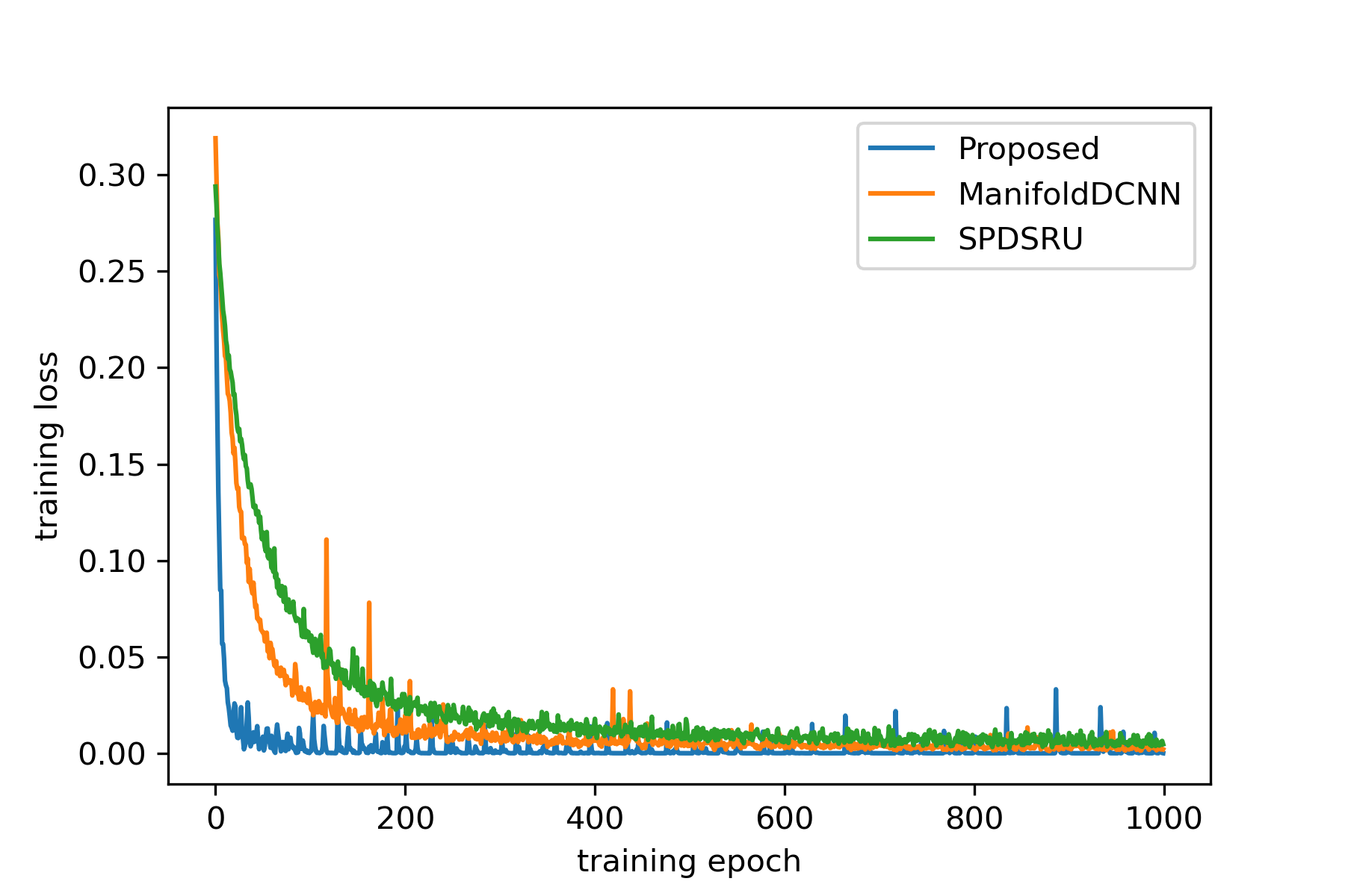
Figure 3: Comparison of the training loss curves of the manifold-based methods over the UCF11 dataset.

5.3.5 Training Speed

Our method uses Cholesky decomposition to map the SPD manifolds into Cholesky space. The Cholesky decomposition greatly reduces the computational costs, allowing us to use the larger SPD matrix than the existing geometric deep-learning methods [34, 52]. Therefore, by using the large SPD matrix, the proposed method could learn various features of the large dimensional input data. We compared the learning curves of three comparative manifold deep-learning methods in Fig. 3. Remarkably, our proposed method showed its convergence faster and more stable than the others.

6 Conclusion

Manifold learning with deep neural networks for SPD matrices is a challenge due to their hard constraints. In this paper, we proposed a novel deep efficient continuous manifold neural network, called ODE-RGRU, by systematically combining GRU and ODE in Cholesky space, and efficiently resolving difficulties related to computational costs in optimization. Specifically, we first reformulated the gating operations in GRU, thus making it work in the Riemannian manifold. Furthermore, to learn continuous geometric feature representations from sequential SPD-valued data, we additionally devised and applied a manifold ODE to the recurrent model. In our extensive experiments on various time-series tasks, we empirically demonstrated its effectiveness and suitability for time-series representation modeling, by achieving state-of-the-art performance for classification, forecasting, and imputation tasks.

Seungwoo Jeong received the B.S. degree in Mathematics and Statistics from Hankuk University of Foreign Studies, Yongin, South Korea, in 2019. He is currently pursuing the Ph.D. degree with the Department of Artificial Intelligence, Korea University, Seoul, South Korea. His current research interests include time-series analysis, brain-computer interface, and machine/deep learning.

Wonjun Ko received the Ph.D. degree in brain and cognitive engineering from Korea University, Seoul, Republic of Korea, in 2022. He was a Data Scientist with SK Hynix Inc., Incheon, Republic of Korea, from 2022 to 2023. He is currently an Assistant Professor at the School of AI Convergence, Sungshin Women’s University, Seoul, Republic of Korea. His current research interests include machine learning, representation learning, and data mining.

Ahmad Wisnu Mulyadi received the bachelor’s degree in computer science education from the Indonesia University of Education, Bandung, Indonesia, in 2010. He is currently pursuing the Ph.D. degree with the Department of Brain and Cognitive Engineering, Korea University, Seoul, South Korea. His current research interests include machine/deep learning in healthcare, biomedical image analysis, and graph representation learning.

Heung-Il Suk is currently a Professor at the Department of Artificial Intelligence and an Adjunct Professor at the Department of Brain and Cognitive Engineering at Korea University. He was a Visiting Professor at the Department of Radiology at Duke University between 2022 and 2023. He was awarded a Kakao Faculty Fellowship from Kakao and a Young Researcher Award from the Korean Society for Human Brain Mapping (KHBM) in 2018 and 2019, respectively. His research interests include causal machine/deep learning, explainable AI, biomedical data analysis, and brain-computer interface. Dr. Suk serves as an Editorial Board Member for Clinical and Molecular Hepatology (Artificial Intelligence Sector), Electronics, Frontiers in Neuroscience, Frontiers in Radiology (Artificial Intelligence in Radiology), International Journal of Imaging Systems and Technology (IJIST), and a Program Committee or a Reviewer for NeurIPS, ICML, ICLR, AAAI, IJCAI, CVPR, MICCAI, AISTATS, etc.

References

- [1] X. Zhen, R. Chakraborty, N. Vogt, B. B. Bendlin, and V. Singh, “Dilated convolutional neural networks for sequential manifold-valued data,” in Proceedings of the IEEE/CVF International Conference on Computer Vision, 2019, pp. 10 621–10 631.
- [2] Y. Zhang, C. Wang, X. Wang, W. Zeng, and W. Liu, “FairMOT: On the fairness of detection and re-identification in multiple object tracking,” International Journal of Computer Vision, vol. 129, no. 11, pp. 3069–3087, 2021.
- [3] J. Devlin, M.-W. Chang, K. Lee, and K. Toutanova, “BERT: Pre-training of deep bidirectional transformers for language understanding,” arXiv preprint arXiv:1810.04805, 2018.
- [4] A. Vaswani, N. Shazeer, N. Parmar, J. Uszkoreit, L. Jones, A. N. Gomez, Ł. Kaiser, and I. Polosukhin, “Attention is all you need,” in Advances in Neural Information Processing Systems, vol. 30, 2017, pp. 5998–6008.
- [5] H. Phan, O. Y. Chén, M. C. Tran, P. Koch, A. Mertins, and M. De Vos, “XSleepNet: Multi-view sequential model for automatic sleep staging,” IEEE Transactions on Pattern Analysis and Machine Intelligence, 2021.
- [6] W. Ko, E. Jeon, S. Jeong, and H.-I. Suk, “Multi-scale neural network for EEG representation learning in BCI,” IEEE Computational Intelligence Magazine, vol. 16, no. 2, pp. 31–45, 2021.
- [7] Z. Che, S. Purushotham, K. Cho, D. Sontag, and Y. Liu, “Recurrent neural networks for multivariate time series with missing values,” Scientific Reports, vol. 8, no. 1, pp. 1–12, 2018.
- [8] P. Schäfer and U. Leser, “Multivariate time series classification with WEASEL+ MUSE,” arXiv preprint arXiv:1711.11343, 2017.
- [9] X. Zhang, Y. Gao, J. Lin, and C.-T. Lu, “TapNet: Multivariate time series classification with attentional prototypical network,” in Proceedings of the AAAI Conference on Artificial Intelligence, vol. 34, no. 04, 2020, pp. 6845–6852.
- [10] G. Li, B. Choi, J. Xu, S. S. Bhowmick, K.-P. Chun, and G. L. Wong, “ShapeNet: A shapelet-neural network approach for multivariate time series classification,” in Proceedings of the AAAI Conference on Artificial Intelligence, vol. 35, no. 9, 2021, pp. 8375–8383.
- [11] Z. Yue, Y. Wang, J. Duan, T. Yang, C. Huang, Y. Tong, and B. Xu, “TS2Vec: Towards universal representation of time series,” in Proceedings of the AAAI Conference on Artificial Intelligence, vol. 36, no. 8, 2022, pp. 8980–8987.
- [12] Y. Rubanova, R. T. Chen, and D. K. Duvenaud, “Latent ordinary differential equations for irregularly-sampled time series,” in Advances in Neural Information Processing Systems, vol. 32, 2019, pp. 5320–5330.
- [13] E. De Brouwer, J. Simm, A. Arany, and Y. Moreau, “GRU-ODE-Bayes: Continuous modeling of sporadically-observed time series,” in Advances in Neural Information Processing Systems, vol. 32, 2019, pp. 7377–7388.
- [14] I. D. Jordan, P. A. Sokół, and I. M. Park, “Gated recurrent units viewed through the lens of continuous time dynamical systems,” Frontiers in Computational Neuroscience, vol. 15, p. 678158, 2021.
- [15] C. Yildiz, M. Heinonen, and H. Lahdesmaki, “ODE2VAE: Deep generative second order ODEs with Bayesian neural networks,” in Advances in Neural Information Processing Systems, vol. 32, 2019, pp. 13 434–13 443.
- [16] P. Kidger, J. Morrill, J. Foster, and T. Lyons, “Neural controlled differential equations for irregular time series,” in Advances in Neural Information Processing Systems, vol. 33, 2020, pp. 6696–6707.
- [17] R. Chakraborty, C.-H. Yang, X. Zhen, M. Banerjee, D. Archer, D. Vaillancourt, V. Singh, and B. Vemuri, “A statistical recurrent model on the manifold of symmetric positive definite matrices,” in Advances in Neural Information Processing Systems, vol. 31, 2018, pp. 8897–8908.
- [18] A. Lou, D. Lim, I. Katsman, L. Huang, Q. Jiang, S.-N. Lim, and C. De Sa, “Neural manifold ordinary differential equations,” in Advances in Neural Information Processing Systems, vol. 33, 2020, pp. 17 548–17 558.
- [19] L. Falorsi and P. Forré, “Neural ordinary differential equations on manifolds,” arXiv preprint arXiv:2006.06663, 2020.
- [20] Y. Yang, D. Krompass, and V. Tresp, “Tensor-train recurrent neural networks for video classification,” in Proceedings of the 34th International Conference on Machine Learning. PMLR, 2017, pp. 3891–3900.
- [21] F. Karim, S. Majumdar, H. Darabi, and S. Harford, “Multivariate LSTM-FCNs for time series classification,” IEEE Transactions on Neural Networks, vol. 116, pp. 237–245, 2019.
- [22] J.-Y. Franceschi, A. Dieuleveut, and M. Jaggi, “Unsupervised scalable representation learning for multivariate time series,” in Advances in Neural Information Processing Systems, vol. 32, 2019, pp. 4650–4661.
- [23] H. Zhou, S. Zhang, J. Peng, S. Zhang, J. Li, H. Xiong, and W. Zhang, “Informer: Beyond efficient transformer for long sequence time-series forecasting,” in Proceedings of the AAAI Conference on Artificial Intelligence, vol. 35, no. 12, 2021, pp. 11 106–11 115.
- [24] G. Zerveas, S. Jayaraman, D. Patel, A. Bhamidipaty, and C. Eickhoff, “A transformer-based framework for multivariate time series representation learning,” in Proceedings of the 27th ACM SIGKDD Conference on Knowledge Discovery & Data Mining, 2021, pp. 2114–2124.
- [25] J. Li, S. Wei, and W. Dai, “Combination of manifold learning and deep learning algorithms for mid-term electrical load forecasting,” IEEE Transactions on Neural Networks and Learning Systems, vol. 34, no. 5, pp. 2584–2593, 2023.
- [26] D. Ding, M. Zhang, F. Feng, Y. Huang, E. Jiang, and M. Yang, “Black-box adversarial attack on time series classification,” in Proceedings of the AAAI Conference on Artificial Intelligence, vol. 37, no. 6, 2023, pp. 7358–7368.
- [27] X. Chen, J. Weng, W. Lu, J. Xu, and J. Weng, “Deep manifold learning combined with convolutional neural networks for action recognition,” IEEE Transactions on Neural Networks and Learning Systems, vol. 29, no. 9, pp. 3938–3952, 2017.
- [28] A. X. Chang, T. Funkhouser, L. Guibas, P. Hanrahan, Q. Huang, Z. Li, S. Savarese, M. Savva, S. Song, H. Su et al., “ShapeNet: An information-rich 3D model repository,” arXiv preprint arXiv:1512.03012, 2015.
- [29] F. Scarselli, M. Gori, A. C. Tsoi, M. Hagenbuchner, and G. Monfardini, “The graph neural network model,” IEEE Transactions on Neural Networks, vol. 20, no. 1, pp. 61–80, 2008.
- [30] T. N. Kipf and M. Welling, “Semi-supervised classification with graph convolutional networks,” arXiv preprint arXiv:1609.02907, 2016.
- [31] M. Moakher, “A differential geometric approach to the geometric mean of symmetric positive-definite matrices,” SIAM Journal on Matrix Analysis and Applications, vol. 26, no. 3, pp. 735–747, 2005.
- [32] S. Jayasumana, R. Hartley, M. Salzmann, H. Li, and M. Harandi, “Kernel methods on the Riemannian manifold of symmetric positive definite matrices,” in Proceedings of the IEEE Conference on Computer Vision and Pattern Recognition, 2013, pp. 73–80.
- [33] A. Kendall and R. Cipolla, “Geometric loss functions for camera pose regression with deep learning,” in Proceedings of the IEEE Conference on Computer Vision and Pattern Recognition, 2017, pp. 5974–5983.
- [34] Z. Huang and L. Van Gool, “A Riemannian network for SPD matrix learning,” in Proceedings of the AAAI Conference on Artificial Intelligence, vol. 31, no. 1, 2017, pp. 2036–2042.
- [35] Y.-J. Suh and B. H. Kim, “Riemannian embedding banks for common spatial patterns with EEG-based SPD neural networks,” in Proceedings of the AAAI Conference on Artificial Intelligence, vol. 35, no. 1, 2021, pp. 854–862.
- [36] R. Chakraborty, J. Bouza, J. Manton, and B. C. Vemuri, “ManifoldNet: A deep neural network for manifold-valued data with applications,” IEEE Transactions on Pattern Analysis and Machine Intelligence, vol. 44, no. 2, pp. 799–810, 2020.
- [37] X. S. Nguyen, L. Brun, O. Lézoray, and S. Bougleux, “A neural network based on SPD manifold learning for skeleton-based hand gesture recognition,” in Proceedings of the IEEE/CVF Conference on Computer Vision and Pattern Recognition, 2019, pp. 12 036–12 045.
- [38] C. Chefd’Hotel, D. Tschumperlé, R. Deriche, and O. Faugeras, “Regularizing flows for constrained matrix-valued images,” Journal of Mathematical Imaging and Vision, vol. 20, no. 1, pp. 147–162, 2004.
- [39] V. Arsigny, P. Fillard, X. Pennec, and N. Ayache, “Geometric means in a novel vector space structure on symmetric positive-definite matrices,” SIAM Journal on Matrix Analysis and Applications, vol. 29, no. 1, pp. 328–347, 2007.
- [40] Z. Lin, “Riemannian geometry of symmetric positive definite matrices via Cholesky decomposition,” SIAM Journal on Matrix Analysis and Applications, vol. 40, no. 4, pp. 1353–1370, 2019.
- [41] Z. Gao, Y. Wu, Y. Jia, and M. Harandi, “Learning to optimize on SPD manifolds,” in Proceedings of the IEEE/CVF Conference on Computer Vision and Pattern Recognition, 2020, pp. 7700–7709.
- [42] R. T. Chen, Y. Rubanova, J. Bettencourt, and D. K. Duvenaud, “Neural ordinary differential equations,” in Advances in Neural Information Processing Systems, vol. 31, 2018, pp. 6572–6583.
- [43] D. Rezende and S. Mohamed, “Variational inference with normalizing flows,” in Proceedings of the 32nd International Conference on Machine Learning. PMLR, 2015, pp. 1530–1538.
- [44] A. Bagnall, H. A. Dau, J. Lines, M. Flynn, J. Large, A. Bostrom, P. Southam, and E. Keogh, “The UEA multivariate time series classification archive, 2018,” arXiv preprint arXiv:1811.00075, 2018.
- [45] J. Lines and A. Bagnall, “Time series classification with ensembles of elastic distance measures,” Data Mining and Knowledge Discovery, vol. 29, no. 3, pp. 565–592, 2015.
- [46] A. P. Ruiz, M. Flynn, J. Large, M. Middlehurst, and A. Bagnall, “The great multivariate time series classification bake off: a review and experimental evaluation of recent algorithmic advances,” Data Mining and Knowledge Discovery, vol. 35, no. 2, pp. 401–449, 2021.
- [47] J. Hu, L. Shen, and G. Sun, “Squeeze-and-excitation networks,” in Proceedings of the IEEE Conference on Computer Vision and Pattern Recognition, 2018, pp. 7132–7141.
- [48] A. v. d. Oord, S. Dieleman, H. Zen, K. Simonyan, O. Vinyals, A. Graves, N. Kalchbrenner, A. Senior, and K. Kavukcuoglu, “WaveNet: A generative model for raw audio,” arXiv preprint arXiv:1609.03499, 2016.
- [49] F. Schroff, D. Kalenichenko, and J. Philbin, “FaceNet: A unified embedding for face recognition and clustering,” in Proceedings of the IEEE Conference on Computer Vision and Pattern Recognition, 2015, pp. 815–823.
- [50] Y.-H. Chen and J.-T. Chien, “Continuous-time attention for sequential learning,” in Proceedings of the AAAI Conference on Artificial Intelligence, vol. 35, no. 8, 2021, pp. 7116–7124.
- [51] L.-P. Xhonneux, M. Qu, and J. Tang, “Continuous graph neural networks,” in Proceedings of the 37th International Conference on Machine Learning. PMLR, 2020, pp. 10 432–10 441.
- [52] D. Brooks, O. Schwander, F. Barbaresco, J.-Y. Schneider, and M. Cord, “Riemannian batch normalization for SPD neural networks,” in Advances in Neural Information Processing Systems, vol. 32, 2019, pp. 15 489–15 500.
- [53] X. Zhen, R. Chakraborty, L. Yang, and V. Singh, “Flow-based generative models for learning manifold to manifold mappings,” in Proceedings of the AAAI Conference on Artificial Intelligence, vol. 35, no. 12, 2021, pp. 11 042–11 052.
- [54] M. Fréchet, “Les éléments aléatoires de nature quelconque dans un espace distancié,” in Annales de l’institut Henri Poincaré, vol. 10, no. 4, 1948, pp. 215–310.
- [55] S. Ioffe and C. Szegedy, “Batch normalization: Accelerating deep network training by reducing internal covariate shift,” in Proceedings of the 32nd International Conference on Machine Learning. PMLR, 2015, pp. 448–456.
- [56] H. Karcher, “Riemannian center of mass and mollifier smoothing,” Communications on Pure and Applied Mathematics, vol. 30, no. 5, pp. 509–541, 1977.
- [57] Y. Chen, A. Wiesel, Y. C. Eldar, and A. O. Hero, “Shrinkage algorithms for MMSE covariance estimation,” IEEE Transactions on Signal Processing, vol. 58, no. 10, pp. 5016–5029, 2010.
- [58] Z. Dong, S. Jia, C. Zhang, M. Pei, and Y. Wu, “Deep manifold learning of symmetric positive definite matrices with application to face recognition,” in Proceedings of the AAAI Conference on Artificial Intelligence, vol. 31, no. 1, 2017, pp. 4009–4015.
- [59] K. Cho, B. Van Merriënboer, C. Gulcehre, D. Bahdanau, F. Bougares, H. Schwenk, and Y. Bengio, “Learning phrase representations using RNN encoder-decoder for statistical machine translation,” arXiv preprint arXiv:1406.1078, 2014.
- [60] E. Hairer, “Solving ordinary differential equations on manifolds,” in Lecture notes, University of Geneva, 2011.
- [61] P. E. Crouch and R. Grossman, “Numerical integration of ordinary differential equations on manifolds,” Journal of Nonlinear Science, vol. 3, no. 1, pp. 1–33, 1993.
- [62] A. Bielecki, “Estimation of the Euler method error on a Riemannian manifold,” Communications in Numerical Methods in Engineering, vol. 18, no. 11, pp. 757–763, 2002.
- [63] K. Kim, J. Kim, M. Zaheer, J. Kim, F. Chazal, and L. Wasserman, “Pllay: Efficient topological layer based on persistent landscapes,” Advances in Neural Information Processing Systems, vol. 33, pp. 15 965–15 977, 2020.
- [64] A. Lou, I. Katsman, Q. Jiang, S. Belongie, S.-N. Lim, and C. De Sa, “Differentiating through the Fréchet mean,” in Proceedings of the 37th International Conference on Machine Learning. PMLR, 2020, pp. 6393–6403.
- [65] J. Liu, J. Luo, and M. Shah, “Recognizing realistic actions from videos “in the wild”,” in Proceedings of the IEEE Conference on Computer Vision and Pattern Recognition, 2009, pp. 1996–2003.
- [66] A. L. Goldberger, L. A. Amaral, L. Glass, J. M. Hausdorff, P. C. Ivanov, R. G. Mark, J. E. Mietus, G. B. Moody, C.-K. Peng, and H. E. Stanley, “PhysioBank, PhysioToolkit, and PhysioNet: components of a new research resource for complex physiologic signals,” Circulation, vol. 101, no. 23, pp. e215–e220, 2000.
- [67] A. Rechtschaffen, “A manual for standardized terminology, techniques and scoring system for sleep stages in human subjects,” Brain Information Service, 1968.
- [68] H. Phan, F. Andreotti, N. Cooray, O. Y. Chén, and M. De Vos, “Automatic sleep stage classification using single-channel EEG: Learning sequential features with attention-based recurrent neural networks,” in Annual International Conference of the IEEE Engineering in Medicine and Biology Society, 2018, pp. 1452–1455.
- [69] H. Phan, F. Andreotti, N. Cooray, O. Y. Chén, and M. De Vos, “Joint classification and prediction CNN framework for automatic sleep stage classification,” IEEE Transactions on Biomedical Engineering, vol. 66, no. 5, pp. 1285–1296, 2018.
- [70] A. Supratak, H. Dong, C. Wu, and Y. Guo, “DeepSleepNet: A model for automatic sleep stage scoring based on raw single-channel EEG,” IEEE Transactions on Neural Systems and Rehabilitation Engineering, vol. 25, no. 11, pp. 1998–2008, 2017.
- [71] H. Phan, F. Andreotti, N. Cooray, O. Y. Chén, and M. De Vos, “SeqSleepNet: End-to-end hierarchical recurrent neural network for sequence-to-sequence automatic sleep staging,” IEEE Transactions on Neural Systems and Rehabilitation Engineering, vol. 27, no. 3, pp. 400–410, 2019.
- [72] A. Asuncion and D. Newman, “Uci machine learning repository,” 2007.
- [73] M. Perslev, M. Jensen, S. Darkner, P. J. Jennum, and C. Igel, “U-time: A fully convolutional network for time series segmentation applied to sleep staging,” in Advances in Neural Information Processing Systems, vol. 32, 2019, pp. 4415–4426.
- [74] H. Seo, S. Back, S. Lee, D. Park, T. Kim, and K. Lee, “Intra-and inter-epoch temporal context network (IITNet) using sub-epoch features for automatic sleep scoring on raw single-channel EEG,” Biomedical Signal Processing and Control, vol. 61, p. 102037, 2020.
- [75] S. Hochreiter and J. Schmidhuber, “Long short-term memory,” Neural Computation, vol. 9, no. 8, pp. 1735–1780, 1997.
- [76] A. L. Maas, A. Y. Hannun, A. Y. Ng et al., “Rectifier nonlinearities improve neural network acoustic models,” in Proceedings of the 30th International Conference on Machine Learning, vol. 30. Citeseer, 2013, p. 3.
- [77] K. Yu and M. Salzmann, “Second-order convolutional neural networks,” arXiv preprint arXiv:1703.06817, 2017.
- [78] H. Phan, F. Andreotti, N. Cooray, O. Y. Chén, and M. De Vos, “DNN filter bank improves 1-max pooling CNN for single-channel EEG automatic sleep stage classification,” in Annual International Conference of the IEEE Engineering in Medicine and Biology Society, 2018, pp. 453–456.
- [79] S. Bai, J. Z. Kolter, and V. Koltun, “An empirical evaluation of generic convolutional and recurrent networks for sequence modeling,” arXiv preprint arXiv:1803.01271, 2018.
- [80] J. Yoon, W. R. Zame, and M. van der Schaar, “Estimating missing data in temporal data streams using multi-directional recurrent neural networks,” IEEE Transactions on Biomedical Engineering, vol. 66, no. 5, pp. 1477–1490, 2018.
- [81] M. Nguyen, T. He, L. An, D. C. Alexander, J. Feng, B. T. Yeo, A. D. N. Initiative et al., “Predicting alzheimer’s disease progression using deep recurrent neural networks,” NeuroImage, vol. 222, p. 117203, 2020.
- [82] M. L. McHugh, “Interrater reliability: the kappa statistic,” Biochemia Medica, vol. 22, no. 3, pp. 276–282, 2012.
- [83] Y. Yang and X. Liu, “A re-examination of text categorization methods,” in Proceedings of the 22nd annual international ACM SIGIR conference on Research and development in information retrieval, 1999, pp. 42–49.
- [84] J. Demšar, “Statistical comparisons of classifiers over multiple data sets,” The Journal of Machine Learning Research, vol. 7, no. 1, pp. 1–30, 2006.
- [85] S. Holm, “A simple sequentially rejective multiple test procedure,” Scandinavian Journal of Statistics, no. 2, pp. 65–70, 1979.