Cadence: A Practical Time-series Partitioning Algorithm for Unlabeled IoT Sensor Streams

Abstract.

Timeseries partitioning is an essential step in most machine-learning driven, sensor-based IoT applications. This paper introduces a sample-efficient, robust, time-series segmentation model and algorithm. We show that by learning a representation specifically with the segmentation objective based on maximum mean discrepancy (MMD), our algorithm can robustly detect time-series events across different applications. Our loss function allows us to infer whether consecutive sequences of samples are drawn from the same distribution (null hypothesis) and determines the change-point between pairs that reject the null hypothesis (i.e., come from different distributions). We demonstrate its applicability in a real-world IoT deployment for ambient-sensing based activity recognition. Moreover, while many works on change-point detection exist in the literature, our model is significantly simpler and can be fully trained in $9$–$93$ seconds on average with little variation in hyperparameters for data across different applications. We empirically evaluate Cadence on four popular change point detection (CPD) datasets where Cadence matches or outperforms existing CPD techniques.

1. Introduction

The number of Internet-of-Things (IoT) and edge devices has exploded in the last decade (Stankovic, 2014; Atzori et al., 2010; Gubbia et al., 2013), providing new opportunities to transform everyday people’s lives. Coupled with advances in learning technologies (Greenwald and Oertel, 2017; Liu et al., [n.d.]), these can transform how people interact with their environment. Although research in this area has also increased dramatically (Nguyen et al., 2019; Jeyakumar et al., 2019; Huynh et al., 2019; Wang et al., 2019), some fundamental challenges remain. A typical machine learning workflow in sensor-based applications starts with unlabeled data. That data is visualized, featurized, and clustered in search of patterns. Typically, labels are obtained, and subsequent sample-label pairs are used to train a classifier. If the data is streaming, this becomes particularly challenging since it is unclear what constitutes the start and end of a training sample. Sensor-based and IoT applications generally follow a workflow where temporal sequence partitioning is a typical pre-processing step . Data acquisition is fast and inexpensive, trivially involving turning on a sensing device and recording measurements. However, partitioning time series to reflect changes observed in the physical world is notoriously difficult, particularly for large-scale systems. It can either be done implicitly through label acquisition from an expert or explicitly using change-point or time series segmentation techniques. In this paper, we focus on time-series partitioning step of sensor-based machine learning pipelines depicted in Figure 1.

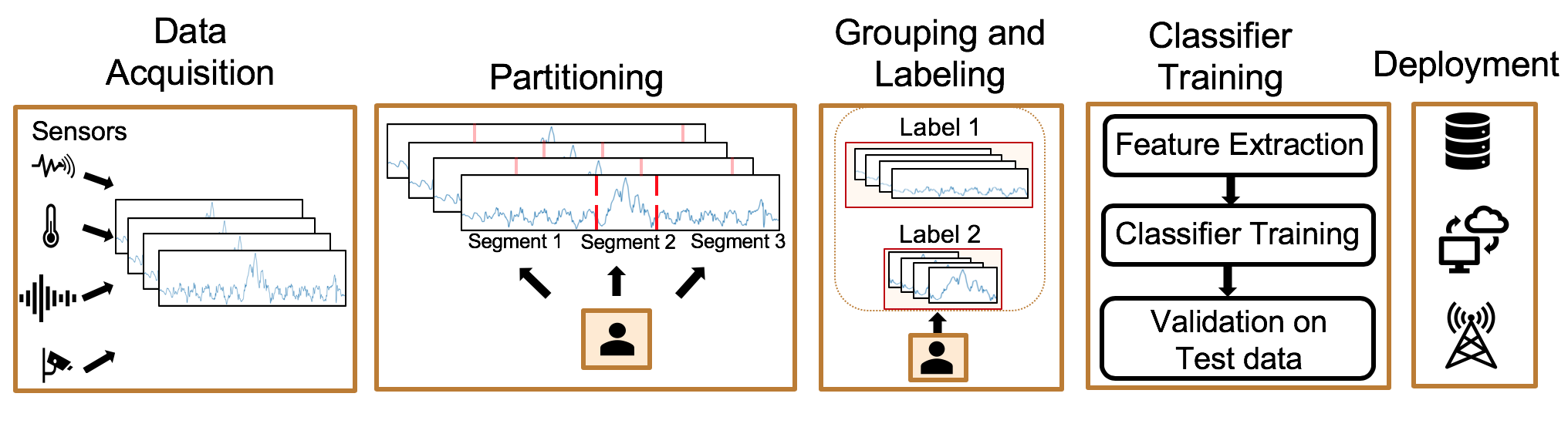
Figure 1. A general machine learning pipeline for sensor-based systems. Note, the partitioning step is crucial and non-trivial, as arbitrary partitioning can lead to arbitrary results (Keogh and Lin, 2005). Applications such as occupancy detection and human activity recognition use manual annotations for partitioning and labeling (i.e. a change in activity or occupancy), increasing labeling effort, and is often inconsistent. Time-series change-point detection can help delineate segments in streaming data without human input, and decrease labeling effort.

Change-point detection (CPD) tries to identify when the probability distribution of a stochastic process changes (Aminikhanghahi and Cook, 2017). While segmentation models a time series using piece-wise functional representations (Keogh et al., 2004), CPD is more useful for learning. Classifiers share similar goals to CPD algorithms. That is, they identify differences in the underlying distribution of the input.

The CPD literature is vast and spans several decades  (Lowry et al., 1992; Basseville and Nikiforov, 1993; Yamanishi and Takeuchi, 2002; Gustafsson, 1996; Kawahara et al., 2007; Idé and Tsuda, 2007; Moskvina and Zhigljavsky, 2003) and has appeared across many disciplines and applications, including finance  (Banerjee and Guhathakurta, 2020; Takayasu, 2015), genetic sequence analysis (Wang et al., 2011), anomaly and fault detection (Yamanishi et al., 2000), and human activity recognition (Ni et al., 2018; Aminikhanghahi and Cook, 2017). There are two broad classes of CPD algorithms: parametric and nonparametric. Parametric approaches make strong assumptions about the data and do not generalize well across different application contexts (Adams and Mackay, 2007; Chowdhury et al., 2012; Nassar et al., 2010). Nonparametric methods are data-driven and based on divergence metrics and kernel functions (Saatçi et al., 2010; Li et al., 2015a), each requiring a unique parameter configuration for a given application context. Deep learning models are most promising for general use but challenging to tune, as hyperparameter search is expensive. Proposed models are complex, making them difficult or impossible to run on edge devices themselves (Chang et al., 2019; Lai et al., 2017; Zhang et al., 2020). Besides, these models are sensitive to the underlying data distribution and the model parameters and thus do not provide a generalized solution.

Developing a data-driven change point detection method that provides computational and sample efficiency and is robust performing across various data domains is non-trivial and poses several challenges that we address in this paper. First, we propose a new way to learn robust time-series features by explicitly learning the similarity (and dissimilarity) between samples through the optimization objective. We show that representations learned in this way are sample efficient and yield better results for change-point detection than computationally expensive, more complex methods. Second, we propose a neural network architecture that learns features from time-series samples by co-training two networks together so that the latent features learned are embedded with similarity characteristics from the samples. This results in a deep embedding learning in latent space that is favorable to change-point detection without distributional assumptions and data-specific hyper-parameter tuning. Third, we show that our method is robust to different parameter choices and yields state-of-the-art performance while being computationally inexpensive. This makes our method, Cadence, a generalized change point detection mechanism for time series data – the most common data type in sensor-based, machine learning applications.

To demonstrate the proposed algorithm’s performance, we evaluate its performance on four empirical datasets (popular in CPD literature) and compare using several state-of-the-art CPD methods as a baseline. We further evaluate it in a real-world scenario for an ambient sensing application and show that Cadence can detect changes in sensor observations and events in the environments without human input. We make the following contributions:

• We propose a new, unsupervised learning approach called Cadence that learns time series embeddings by learning the similarity (and dissimilarity) between samples by incorporating MMD in the objective function.

• We show that it is sample efficient and much easier to train than state-of-the-art techniques.

• Cadence offers a generalized change point detection algorithm based on learned embeddings that does not require distributional assumptions and yields robust performance for different parameter settings.

• We show Cadence’s use in a real-world IoT application and present an empirical evaluation of Cadence on four popular CPD datasets where Cadence significantly outperforms existing CPD techniques.

Our algorithm is developed as a Python library and will be released as an open-source tool for use in end-to-end sensing applications.

The rest of the paper is organized as follows. We position the proposed approach to fill the gap in the existing change-point detection literature in Section 2. Sections 3 and 10.7 discuss the motivation behind change-point detection in the machine learning pipeline and the design rationale, respectively. In Sections 5,  6, and  7, we discuss the problem formulation of change-point and the two critical components of our method; kernel two-sample test and auto-encoder based feature learning, respectively. We demonstrate its practical deployability in a real-world application for ambient-sensing in Section 8. In Section 9, we describe the experimental evaluation procedure of the proposed approach. In Section 10, we show that Cadence outperforms state-of-the-art techniques and we conclude by discussing limitations of Cadence and future works in Section 11.

2. Related Work

In this section, we position our work in the context of previous works in the literature on change-point detection and kernel two-sample tests.

2.1. Change Point Detection

Many works in change-point detection are based on comparing probability distributions of time-series samples over past and current intervals (Basseville and Nikiforov, 1993; Gustafsson, 1996). In these methods, the common strategy is to detect a candidate change point when the two samples become significantly different by some statistical difference measure and the system issues an alarm for a change point (Basseville and Nikiforov, 1993; Willsky and Jones, 1976). Gustaffsson et al. (Gustafsson, 1996) introduced marginalized likelihood ratio-based difference measure to eliminate the pre-defined threshold and reduced computational complexity for generality and robustness. Similar to them, our work refrains from setting a dataset-specific threshold.

Kawahara et al. utilized (Kawahara et al., 2007) subspace models, where a subspace of the data space is discovered and the distance between the sub-spaces is utilized as a difference measure to identify changes. While the methods in this line are computationally efficient, they require a pre-designed time-series parametric model to form the sub-space (Idé and Tsuda, 2007; Moskvina and Zhigljavsky, 2003). Both state-space models and probability distribution methods rely on assumptions about parameters such as mean, variance, and the spectrum of underlying distributions for tracking changes. In our proposed model, we make no such assumptions about distribution parameters. Instead, we track changes in the underlying distribution of the data from features learned via a deep neural network.

As an alternative to parametric assumptions, non-parametric techniques such as density estimation has been used to identify changes in the literature. However, the performance of such methods degrades significantly for high dimensional data (Härdle et al., 2004). To ease this problem (Sugiyama et al., 2012) proposed direct density ratio estimation method, where the ratio of probability densities are estimated without actual calculation of probability density. Following this line, several techniques KLIEP (Sugiyama et al., 2008), uLSIF (Kanamori et al., 2009), RuLSIF (Liu et al., 2013) have been introduced for change detection under non-parametric setting. Liu et al. (Liu et al., 2013) used relative density ratio as a difference measure between samples to detect the change, but its performance is affected by the choice of hyperparameters such as window length and sample size. (Aminikhanghahi and Cook, 2017; Aminikhanghahi et al., 2018) used a non-parametric change detection approach using Separation distance as the difference measure, but it requires pre-defined feature calculation to apply the algorithm for change-point detection.

(Lee et al., 2018; De Ryck et al., 2020) explored change point detection using auto-encoders, but their performance for different datasets is largely influenced by window size and parameter settings. Sinn et al. (Sinn et al., 2012) used Maximum Mean Discrepancy (MMD) as the difference between the ordinal pattern in distribution (order structure in time series values) before and after a change-point under the assumption that the underlying time series is monotonically increasing or decreasing and for detecting multiple change-points requires iteratively applying the method to different blocks of the time series. The work in this paper is closely related to this line of work. While we use MMD as the score of change point possibility measure, we focused on computing change-point scores using kernel two-sample test on features learned from an autoencoder-based neural network.

2.2. Kernel Two Sample Test

Kernel two-sample test has been useful for statistical tests to identify the difference between two probability distributions. The two-sample tests are performed based on samples drawn from two probability distributions using a test statistic as the difference between two samples. Harchaoui et al. (Harchaoui et al., 2008) used a test statistic based upon maximum kernel Fisher discriminant ratio as a measure of homogeneity between segments in hypothesis testing. Along this line, Gretton et al. (Gretton et al., 2012a) introduced Maximum Mean Discrepancy (MMD) and non-parametric statistical tests based on MMD as a test statistic that is free from distribution assumptions.

MMD-based kernel two-sample test has been effective in change point detection literature (Zou et al., 2014; Harchaoui et al., 2008; Li et al., 2015b). However, the performance of these kernel methods requires tuning of the bandwidth parameter to obtain optimal performance from kernel measures. In (Gretton et al., 2012a, b) Gretton et al. presented a bandwidth parameter selection strategy for kernel using median value, which is a simple heuristic for good performance without theoretical validation, as shown by Ramdas et al. (Ramdas et al., 2015). In (Gretton et al., 2012b), Gretton et al. showed that better kernels can be learned by optimizing test power, which can be less effective in CPD problems with insufficient samples. Chang et al. (Chang et al., 2019) approached this problem by generating additional samples to mitigate the problem of insufficient samples and optimize test power towards better kernel learning. However, training generative models are computationally expensive and are thus of limited use in practice.

We take inspiration from (Liu et al., 2013) and compare subsequent samples based on a test statistic to identify a change in the distributions. We use Maximum Mean Discrepancy (MMD) as a test statistic as in (Chang et al., 2019). However, instead of generating additional samples towards kernel learning, we learn latent representations for change point detection from the samples by a deep neural network-based optimization. Our approach provides a generalized learning paradigm with simpler network architecture and faster training while achieving better detection performance.

3. Motivation

A typical machine learning pipeline has multiple phases: 1) data acquisition, 2) data labeling, 3) classifier training and testing, and 4) deployment and execution. We argue that in sensor-based, streaming machine learning applications, the transition from step 1 to step 2 is particularly challenging:

1. Most sensor data are time-series in nature, so the labeler can approximately delineate boundaries between events only if the data is put in the proper semantic context.

2. Raw sensor observations do not typically provide enough context, so labels are generated either by labeler in-situ or recorded via a contextually richer sensing modality (i.e., video/audio) and labeled a posteriori through manual annotations.

3. A standard solution is to pick a fixed, sliding window over the raw streams and acquire labels.

4. The exact delineation boundary for streaming data is not well defined (i.e., two different labelers may delineate the data in similar but unequal ways).

These challenges differentiate a standard machine learning pipeline from a streaming sensor-based one, illustrated in Figure 1.

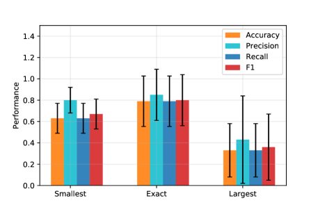
Figure 2. Classifier performance on the Beedance dataset under different delineation boundary sizes. Here, we create samples from the time series by sliding a fixed size window, where under Smallest and Largest condition window size is selected from the smallest and largest true segment present in the data. Under Exact condition, all samples are created from true segment boundaries in data based on labels. Selecting an arbitrarily small or large window introduces noise into individual samples and can influence the classifier’s performance.

We make several observations of the pipeline presented in the figure. First, as the exact delineation boundary for streaming data is arbitrary, human inspection involves high effort and high cost. Humans are error-prone and can misidentify event transitions, label them inconsistently, or may miss them altogether. Second, the context modality must be synchronized with the sensing modality for proper labeling. A delay in the measurement platform (i.e., network, processing) can cause a delay between the physical observation of an event and when it is recorded. Third, poor delineation can lead to poor classifier performance and can cause information leakage between events. The chosen window size influences the classifier’s performance as selecting an arbitrarily small or large window introduces noise into individual samples. A window too small may not contain sufficient relevant information about an event; a window too large may contain information about multiple events instead of a single event—this can result in biasing the classifier’s view of the input distribution.

We make this observation in Figure 2, whereby we measure a classifier’s performance as we change the boundaries that define discrete samples. Note, there is a drop in performance for samples created using a sliding window of fixed size. We also observe that performance improves when the actual segment boundaries define samples. (Sadri et al., 2018; Aminikhanghahi and Cook, 2017) made a similar observation that temporal segmentation as a pre-processing step in conjunction with a prediction or classification model leads to performance improvement in comparison to using a fixed-length sliding window, which is the common practice in many application areas including activity recognition (Ma et al., 2021; Bai et al., 2020; Tang et al., 2021; Abedin et al., 2021). We highlight some of these applications explored in recent literature in Table 1 that utilizes time-series partitioning procedure. More perniciously, Keogh et al. (Keogh and Lin, 2005) assert that features extracted from arbitrary segments by sliding static windows result in arbitrary results. This observation highlights the importance of finding good, representative sample boundaries in continuous measurements to capture physical events’ dynamics.

In many real-world sensing applications (Pan et al., 2019), statistical properties of events change over time and expose the system to concept-drift (Janardan and Mehta, 2017; Webb et al., 2016) and reduced performance for machine learning applications, as the training samples deviate from the observed ones over time. There is a need to incorporate change point detection techniques to enable continuous-learning applications. However, while complex models (Lai et al., 2017; Chang et al., 2019; Zhang et al., 2020) may outperform simpler ones, they are difficult to use in real systems due to their computation cost. Most IoT application developers desire an easy to train neural network, robust to different parameters and high performing across various application data. It relieves them from acquiring expertise in the underlying model to tune it for their specific purpose properly.

Category	Paper	Application Area
Activity Recognition	(Aminikhanghahi and Cook, 2017)	Activity detection in smart home using sensors
	(Wang and Zheng, 2018)	Activity recognition using RFID
	(Noor et al., 2017)	Activity recognition from accelerometer data
	(Kwon et al., 2020)	Activity recognition using virtual sensor extracted from video
Event Detection	(Guo et al., 2018)	Workout event detection using WiFi
	(Ohara et al., 2017)	Event detection of indoor objects using WiFi
	(Li, [n.d.])	Daily life event segmentation using wearable sensors
	(Saeed et al., 2021)	Physiological event detection using WiFi and wearable sensor
Other	(Huang et al., 2019)	User identification and authentication using RFID
	(Sarker et al., 2018)	Smartphone usage behaviour analysis
	(Bonacina et al., 2020)	Industrial plant status monitoring using temperature sensor

Table 1. Some application areas in recent literature that use time series partitioning in the pipeline

4. Design Rationale

4.1. Properties of Practical CPD Algorithms

Although partitioning is an essential step for time-series-based machine learning applications, the existing solutions do not offer the properties to make them feasible for real-world applications. Here, we describe the properties we need in a changepoint detection method to support real-world applications:

• Property 1: Ease of use. CPD techniques should be usable without the need for application domain-specific knowledge or strong assumptions about the underlying data distribution. Most approaches in parametric CPD make strong assumptions about data distribution (Adams and MacKay, 2007; Nassar et al., 2010), and even non-parametric ones are dependent on parameter choices such as window size and the number of training samples (Liu et al., 2013; Sugiyama et al., 2012; Li et al., 2015b).

• Property 2: Computational efficiency. A CPD library needs to provide satisfactory results while minimizing computational cost and runtime. While some approaches are not parameter-dependent and can achieve good performance, they are computationally expensive and are thus infeasible for practical purposes (Chang et al., 2019; Liu et al., 2018).

• Property 3: Performance. CPD techniques should accurately identify changes in the data distribution. A well-performing algorithm may achieve its precise performance due to data-specific parameterization or computational overhead for complex modeling purposes  (Chang et al., 2019), but have limited general use. On the other hand, relaxing the first two properties may degrade detection performance and become unreliable in practice.

We now discuss the design choices we make in our proposed approach, Cadence, to ensure these properties.

4.2. Design Discussion

Our change point detection scheme computes a dissimilarity score between two consecutive segments in time series such that this score can act as a probability of change point. There are several design choices involved in this process to ensure that the mechanism exhibits the properties in Section 4.1.

Maximum Mean Discrepancy. We utilize Maximum Mean Discrepancy (MMD) to measure the dissimilarity between the segments. MMD is a probabilistic distance measure that has been useful in non-parametric hypothesis testing (Gretton et al., 2012a). In our proposed technique, we perform hypothesis testing to determine change points in a two-sample test setting using Maximum Mean Discrepancy (MMD) as the test statistic. We perform the test between two consecutive segments (null hypothesis of they come from the same distribution vs. alternate hypothesis of they come from different distributions). While, there are other measures for the distance between two distributions such as Kullback-Leibler (KL) divergence (Pérez-Cruz, 2008), MMD is attractive for our use case for several reasons. First, it is a non-parametric distance measure, which relieves from parameter choice for estimation (Property 1). Second, MMD represents the distance between probability distributions as the distance between mean embeddings of features and can be easily empirically computed with a given number of samples (Property 2). As we are interested in MMD between latent embeddings of two segments to be used as change-point score, the non-negative, symmetric, and non-parametric properties of MMD provide a solution that is easy to compute and high-performing. Based on these advantages, we choose MMD over other distance measures such as KL divergence as our dissimilarity metric.

Autoencoder. We choose a stacked auto-encoder to learn the feature representations from time-series samples in a lower dimension space and calculate MMD in that space instead of calculating in data space. MMD-based change point detection measures the distance by applying a function on the samples to learn feature embeddings. Chang et al. (Chang et al., 2019) found that learning a better representation can help hypothesis testing-based change point detection compared to performing the test in the original data space. However, their approach based on generating additional samples is computationally expensive (Property 3).

On the other hand, with Autoencoder, we use gradient descent via back-propagation to learn the representation that is suitable for detecting changes between the samples, instead of calculating MMD between two samples in a linearly embedded space as in principal component analysis (PCA) or non-negative matrix factorization (NMF). Recent research has shown that auto-encoders are capable of producing meaningful and well-distinguished representations on real-world datasets (Vincent et al., 2010; Le, 2013; Hinton and Salakhutdinov, 2006) and exhibit denoising property in feature learning [72], which can be useful for noisy real-world time-series from IoT (Property 2). Furthermore, autoencoder training’s unsupervised nature facilitates learning representations without explicitly utilizing labels.

We experimented with several other models described in the literature, including a variational autoencoder (Kingma and Welling, 2013) and a variational recurrent neural network (Chung et al., 2015). Surprisingly, despite its simplicity, we found autoencoders outperform more complex models across various datasets. It is also simpler to train.

4.3. Caveats and Shortcomings

Before describing our proposed method, we explain some additional design choices we make in our method.

Window. In our proposed method, we use a sliding window to create segments for testing the hypothesis for change point. A sliding window may raise concern among the readers as the window size is a parameter choice, and this choice can influence algorithm performance. Note that the window size dictates the length of a segment. We compare segments by calculating the dissimilarity between consecutive segment pairs (Note Figure 3). However, our window-size choice does not dictate the start and end of an input sample used downstream in the rest of the processing pipeline. Here, we are interested in finding a homogeneous sample for an ML application, where the sample represents a single event or activity. To perform that comparison, we slide a window across the entire stream to compare consecutive segments created by the process above and use the dissimilarity to identify the start and end of a sample.

However, the fixed window size can still influence the algorithm’s sensitivity to events. We choose a window size of 25 timesteps for all of our experiments and experimentally explore how the choice influences performance in Section 10.4.

Figure 3. By sliding window $w$, pairs of past segment ${x_{L}}=\{{y_{t-w}},\dots,{y_{t-1}}\}$ and current segment ${x_{R}}=\{{y_{t}},\dots,{y_{t+w-1}}\}$ are compared to detect change point at every incoming time point. Note that, the objective of this window is to create non-overlapping segments for comparing their dissimilarity and use it as change-point probability at $t$ in two-sample test.

Threshold. We use the maximum mean discrepancy (MMD) score between consecutive segment pairs as the changepoint score. We report our proposed method’s performance using Area Under Curve Score (AUC) from true-positive rate (TPR) and false-positive rate (FPR) obtained using this changepoint score. However, to partition a time series into segments based on the obtained changepoint score, we need to set a threshold on the score. While finding an adaptive threshold that works well across different datasets is outside of this paper’s scope, in our experiments, we empirically observed that using a threshold of 40% of the maximum change point score provides good detection performance.

5. Problem Formulation

In this section, we formulate the problem of change point detection for time series. Let us consider a time series of $d$-dimensional observations $Y=\{{y_{1}},{y_{2}},{y_{3}},\dots y_{t},\dots\}$, where ${y_{t}}\in{\mathbb{R}^{d}}$. We create segments of window size $w$ and treat each segment as a single sample instead of a single $d$-dimensional observation. We follow the previous works in the literature in this choice (Liu et al., 2013; Sugiyama et al., 2008) as this captures the time-dependent information in the observations. Our objective is to detect a change point, where the observations undergo change.

Towards the goal of change point detection, we consider two consecutive segments of size $w$ at time $t$; past segment $x_{L}$ and current segment $x_{R}$. Our change point detection scheme is to compute a dissimilarity score between these two consecutive segments such that this score can act as a probability of change point at time $t$. Specifically, we want to leverage the dissimilarity score to answer whether samples ${x_{L}}$ and ${x_{R}}$ are from different distributions and hence decide whether the current time $t$ is a change point. Here, $t$ is the first time-point in the current segment marking the boundary between the two segment pairs. We create such segment pairs by a sliding window approach for the entire time series. This results in two matrices of past segments ($X_{L}$) and current segments ($X_{R}$). The dissimilarity between each pair allows us to compute change point scores for ${{t},{t+1},{t+2},{t+3},\dots}$ as shown in Figure 3.

Figure 3 illustrates the change point detection strategy for one-dimensional time series. For multi-variate time series, we concatenate segments in all dimensions into one segment while maintaining the order of time. This allows our strategy to be valid regardless of the number of dimensions under consideration instead of detecting changes in each dimension individually. In the next section, we introduce the dissimilarity score used for measuring change point probability.

Constraints. Notice that following the previous literature (Liu et al., 2013; Sugiyama et al., 2008; Chang et al., 2019), we create samples of window size $w$ to capture time-dependent information in our samples. In this setting, the method needs to have a specific number of observations available to create samples (which is dependent on the size of the window) for computing dissimilarity between sample pairs. As a result, the method cannot detect changes as soon as they occur as considered in the online changepoint detection setting. However, the smaller the window size is, the faster it can respond to a changepoint in inference mode (when a trained model is used to find change points on new data). Furthermore, we made piece-wise i.i.d. assumption regarding the segments created in this setting following the previous works (Harchaoui et al., 2008; Kawahara et al., 2007; Li et al., 2015b). However, in many settings, samples may not follow such assumptions and can follow non-i.i.d autoregressive process. We formulate the problem of change point detection for time series under these constraints and extending beyond this setting can be interesting which we leave for future work.

6. MMD for two-sample test

6.1. Two-sample Test

We utilize the concept of Maximum Mean Discrepancy (MMD) to measure the dissimilarity between the segments, ${x_{L}}$ and ${x_{R}}$. Maximum Mean Discrepancy is a probabilistic difference measure that is used for the two-sample test. In a two-sample test problem, a statistical test is performed under the null hypothesis that the probability distribution of the two samples is the same against the alternative hypothesis that the probability distribution of the samples is different.

Let us consider sample $X=\{{x_{1}},{x_{2}},\dots,{x_{m}}\}\sim P$ and sample $Y=\{{y_{1}},{y_{2}},\dots\ ,{y_{n}}\}\sim Q$ are i.i.d and drawn from distributions $P$ and $Q$ respectively. The definition of two-sample test can be formally established as:

${H_{0}}:P=Q$, samples X and Y are from same distributions.

${H_{A}}:P\neq Q$, samples X and Y are from different distributions.

Ideally, in a two-sample test, the test statistic should be such that when this measure is large, the samples are likely from different distributions, $P\neq Q$. On the other hand, the statistic becomes 0 if and only if $P=Q$. The closer the test statistic exhibits this behavior, the less susceptible it is to Type I and Type II errors.

6.2. MMD as test statistic

Maximum Mean Discrepancy (MMD) has been used in the literature as the two-sample test statistic (Harchaoui et al., 2008). MMD is defined as the difference between the mean embedding of the two samples. The hypothesis of two distributions $P$ and $Q$ being different is tested based on the samples drawn from each of them. Following the notations in (Gretton et al., 2012a, b, 2009), MMD between two distributions $P$ and $Q$ can be thus expressed as distance between the mean embeddings of $P$ and $Q$ in the following way,

(1) $${MMD}^{2}({P},{Q})={{M_{k}}}({P},{Q})={{\parallel{\mu_{P}}-{\mu_{Q}}\parallel}^{2}}$$

Given a kernel $k$ in the embedding space and the samples from $P$ and $Q$ are $X$ and $Y$, MMD can be written in terms of kernel functions as following,

(2) $${{M_{k}}}({X},{Y})=\mathop{\mathbb{E}_{P}}[{k(x,x^{\prime})}]-2\mathop{\mathbb{E}_{PQ}}[{k(x,y)}]+\mathop{\mathbb{E}_{Q}}[{k(y,y^{\prime})}]$$

where $x^{\prime}$ and $y^{\prime}$ are an independent copy of $x$ and $y$ from the distributions $P$ and $Q$ respectively. It has been demonstrated in (Nishiyama and Fukumizu, 2016) that for both Gaussian and Laplace kernels, ${M_{k}}({P},{Q})=0$ if and only if ${P}={Q}$. Additionally, both kernels exhibit properties of a characteristic kernel where ${M_{k}}({P},{Q})$ is non-negative.

The change point detection problem can be simplified into a binary classification problem where MMD at each time step acts as the change point probability score for the corresponding timestamp. ${M_{k}}({P},{Q})>0$ between $x_{L}$ and $x_{R}$ thus denotes the probability of time step $t$ being a change point. Note that, the two-sample test is designed to inform on the hypothesis of two samples coming from the same distribution based on ${M_{k}}({P},{Q})=0$. We leverage its notation for the change-point detection setting by using the MMD statistic as a change point probability.

In practice, ${M_{k}}({P},{Q})$ is estimated using finite samples from the two distributions $P$ and $Q$ through their kernel mean embedding. However, the test power is limited by the finite samples available for the estimation, as change points are rare in most cases.

6.3. Kernel Choice for MMD

The motivation for the choice of kernel can depend on problem complexity and the information to be extracted from the data. MMD utilizes the difference between the embeddings of the samples to perform the two-sample test. Hence, the kernel or similarity metric used in the test is crucial to its performance (Gretton et al., 2012a). Recall that the two-sample test should ensure that samples from unlike distributions should be distinguished with high probability. This minimizes Type II error, or false negative rate, which occurs if the test fails to show a difference when there is one. Similarly, the test statistic should be 0 (or very close to 0) when samples from the same distributions are compared.

The family of radial basis function (RBF) kernels exhibits such behavior. An RBF kernel is defined as,

(3) $${k(x,y)}=exp(-\gamma{\|x-y\|}^{2})$$

where the value of $\gamma$ is an adjustable parameter that provides sensitivity. The common heuristic to choose the value of gamma for RBF kernels in the literature is to use the median value (Schölkopf et al., 2002). However, the median heuristic does not guarantee maximum power and optimal performance of test statistics. Note that, the RBF kernel function is a non-linear euclidean distance whose value depends on the choice of $\gamma$. While the value of $\gamma$ contributes to the non-linear nature of this distance measure and the performance of the kernel, it requires hand-tuning for optimal performance depending on the data complexity and problem domain.

Considering $x=x^{\prime}$ and $y=y^{\prime}$ in (2), and combining (2) and (3), we get,

(4) $${{M_{k}}}({X},{Y})=\mathop{\mathbb{E}_{P}}[{k(x,x)}]-2\mathop{\mathbb{E}_{PQ}}[{k(x,y)}]+\mathop{\mathbb{E}_{Q}}[{k(y,y)}]$$

As a result, the first and third term in (4) becomes 1, which results in the value of ${{M_{k}}}({X},{Y})$ being dependent on the 2nd term only. There can be two cases here:

Case 1: $x=y:k(x,y)=1\rightarrow{}{{M_{k}}}({X},{Y})=0$

Case 2: $x\neq y:k(x,y)<1\rightarrow{}{{M_{k}}}({X},{Y})>0$

Note that this lays the foundation for test statistics suitable for the two-sample test in the change-point detection setting. In the next section, we discuss an embedding learning method via a deep neural network that learns features useful towards change point detection.

7. Deep Embedding Learning

LeCun et al. (LeCun et al., 2015) show that deep learning algorithms are in fact representation learning frameworks with representations lying on multiple levels, which are obtained by multi-layer non-linear transformation of the input. While many works have been done in the computer vision and natural language processing literature that have focused on learning representations for a specific task, relatively fewer works have focused on unsupervised feature learning from raw time series for change point detection.

7.1. Feature Learning For Change Point Detection

The foundation of MMD-based change point detection is grounded on measuring the distance between the samples by applying some kernel function on the samples that projects them in a new vector space. However, the feature space learned in this method is dependent on the number of samples available. Chang et al. (Chang et al., 2019) approached this problem by generating additional samples through a generative network to mitigate the problem of insufficient samples. Despite the computational complexity, it is clear from their findings that learning a better representation can help in the two-sample test-based change point detection in comparison to performing the test in the original data space. Which leaves us with the following question: Can we learn a feature representation from time-series data using deep neural networks, to detect change points in an unsupervised way, without generating new samples?

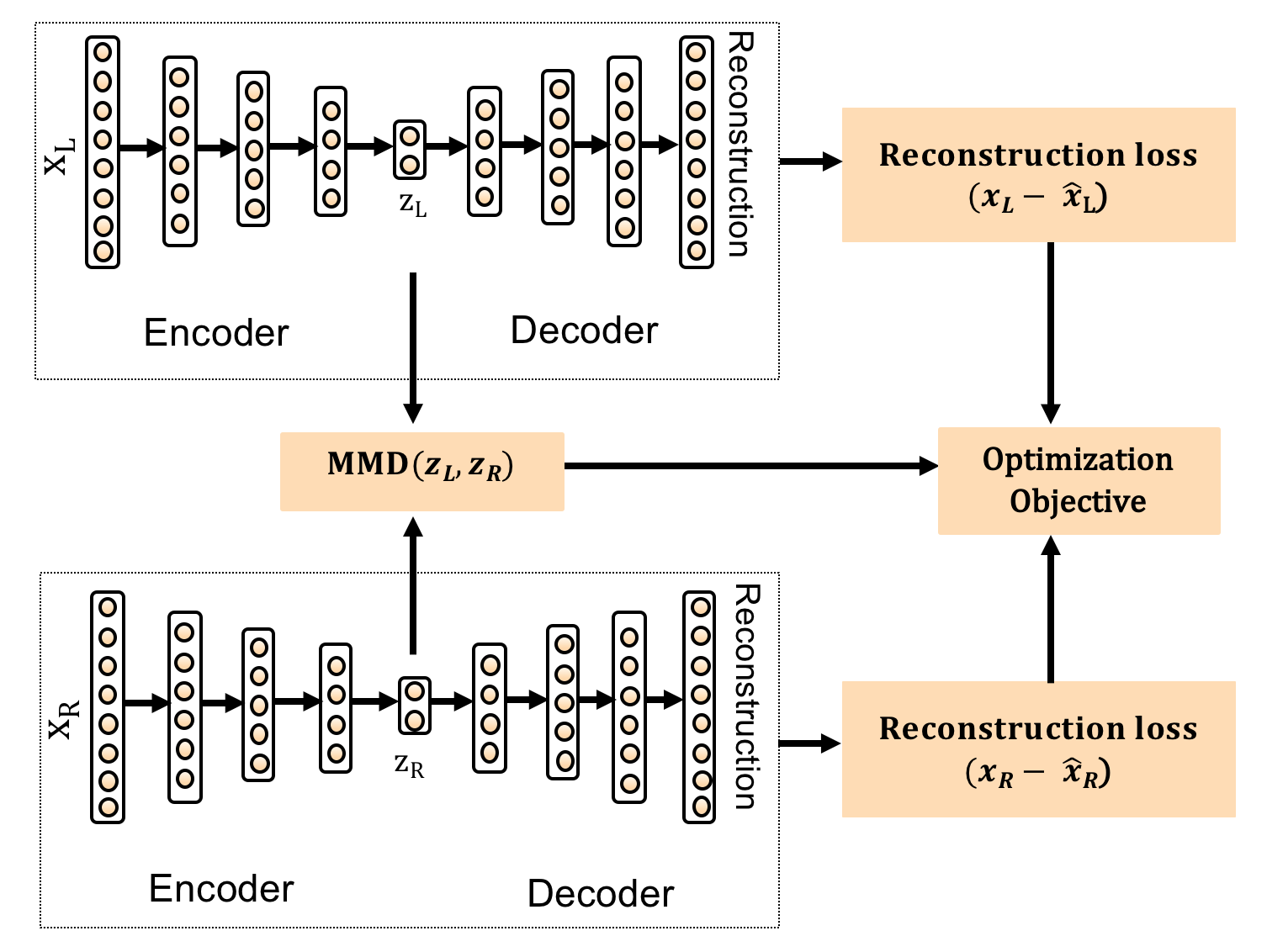
Figure 4. The architecture of the autoencoder network used in Cadence. We used three fully connected hidden layers with ReLU activation. For optimization, we used Adam optimizer and the learning rate was set to 0.0001. More implementation details are explained in Section 9.4

7.2. Auto-encoder

We propose to use a stacked auto-encoder to learn the feature representations from the data space to a lower dimension space. An auto-encoder is a pair of functions ($f$, $g$) designed to encode and decode data signals from an underlying domain. It takes an input ${x}$ = {${x_{1}},{x_{2}},{x_{3}},\dots,{x_{d}}\}\in{\mathbb{R}^{d}}$ and maps it to a hidden representation ${z}$ = {${z_{1}},{z_{2}},{z_{3}},\dots,{z_{d^{\prime}}}\}\in{\mathbb{R}^{d^{\prime}}}$ through a deterministic mapping between the input and the code.

The latent representation $z$ is mapped back to a reconstructed input $\hat{x}=g_{\theta^{\prime}}(z)$ = $\phi(W^{\prime}x+b^{\prime})$ in the input space with parameters $\theta^{\prime}=\{W^{\prime},b^{\prime}\}$. The parameters of the autoencoder {$\theta,\theta^{\prime}$} are optimized to minimize the $l_{2}$ reconstruction error $\mathcal{L}$($\boldsymbol{x}$, $\boldsymbol{\hat{x}}$):

(5) $$\theta,\theta^{\prime}={argmin_{\theta,\theta^{\prime}}}\mathcal{L}(x,\hat{x})$$

Here, $\mathcal{L}$ is a loss function which is a measure of the discrepancy between input $\boldsymbol{x}$ and its reconstruction $\boldsymbol{\hat{x}}$ over all available training samples.

7.3. Learning Representation for Change Point

In our architecture, we apply a non-linear transformation to the data X and map it to lower dimension feature space ${Z},{f_{\theta}}$ $\colon$ ${X}$ $\rightarrow{Z}$, where $\theta$ are the learnable parameters. The optimization objective should allow learning such features that maximize the dissimilarity between the segments that are from different distributions in the latent space $Z$. Figure 4 shows the neural network architecture used in Cadence.

Objective Function Rationale. Reconstruction loss is the commonly used loss function in neural network parameterization, defined as the squared loss between the input $x$ and its reconstructed output $\hat{x}$, ${{\|x-\hat{x}\|}^{2}}$. However, reconstruction loss minimizes towards better reconstruction output, whereas we are interested in better separation between segments that are from different distributions.

Towards this goal, we use an additional loss function to learn features useful to the change point detection task, which we name as MMD loss. It is defined as ${MMD}({z_{L}},{z_{R}})$, where ${z_{L}}$ and ${z_{R}}$ are the latent representation of the past and current segments ${x_{L}}$ and ${x_{R}}$ learned in the optimization process. Note that, our objective is to learn a representation through the training that separates the dissimilar segments better in the learned feature space. While two-sample test demands for MMD to be large ($>0$) to detect a change-point, maximizing MMD between the pairs directly will maximize the distance between samples for both when P = Q (same distribution) and P $\neq$ Q (different distribution). This will increase the false positive rate in the test statistic and will fail to achieve the change point detection goal.

Hence, we use MMD loss as an optimization objective that allows learning such features so that both reconstruction loss and MMD are minimized for segment pairs. This strategy is motivated by the intuition that MMD contribution in the loss function (and optimization) comes from only pairs from different distributions. One reason for this strategy’s effectiveness can be minimizing MMD loss helps the latent space towards better segmentation in conjunction with reconstruction objective, whereas explicitly maximizing MMD loss moves further away from reconstruction objective space. The magnitude of MMD between the pairs in the lower dimension is much less than the reconstruction loss (between the sample and its reconstructed approximation). Hence, the total loss function value per epoch is dominated by reconstruction loss. We therefore use a weighting factor $\beta$ to MMD to balance its effect on the loss function value (please see section 9.4 and 10.2 for details on the choice of $\beta$ value).

The objective function for our algorithm (Algorithm 1) thus becomes, Reconstruction loss + MMD loss

(6) $${{\|x_{L}-\hat{x_{L}}\|}^{2}}+{{\|x_{R}-\hat{x_{R}}\|}^{2}}+{\beta}{M_{k}}({z_{L}},{z_{R}})$$

1

Input : $w$ window size, $\alpha$ learning rate, ${n_{c}}$ number of iterations

2

Output : change point scores

3

4Learning

5while ${M_{k}}({Z^{L}},{Z^{R}})<\epsilon$ do

6       for $t=1,\dots n_{c}$ do

7             Sample a minibatch ${X_{t}}={({X^{L}_{t}},{X^{R}_{t}})}$;

8            

9            gradient $(\theta)$ $\leftarrow{}$ $MSE$ ($X^{L}$, $\hat{X^{L}}$) + $MSE$ ($X^{R}$, $\hat{X^{R}}$) + $M_{k}(Z^{L},Z^{R})$;

10            

11            $\theta$ $\leftarrow{}$ $\alpha\cdot$ Adam ($\theta$, gradient $(\theta)$);

12            

13       end for

14      

15 end while

16

17Inference

18feature space mapping, ${f_{\theta}}$ $\colon$ $X^{L},X^{R}$ $\rightarrow$ ${Z^{L},Z^{R}}$;

19

20${M_{k}}({Z^{L}},{Z^{R}})\sim$ change point scores;

21

22return change point scores;

Algorithm 1 our proposed algorithm

For change point detection, we train the autoencoder in the learning phase (Algorithm 1) to learn a latent feature representation from each sample pair specifically with the objective function in (6). In the inference phase, we use the trained network to project incoming sample pairs in the latent space and perform a two-sample test based on the MMD computed in the latent space.

Change Point Detection. To identify change points, we first apply a smoothing filter on this score and then use the resultant score as change point probability for each time point. From this set of probabilities, we find local maxima points using a threshold of 40% of the maximum change point score. We empirically observed that this threshold has worked well for the datasets used in the experiments. This relieves from relying on a user-defined threshold decided from domain-specific knowledge.

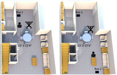
Figure 5. Data collection setup using multiple sensor boxes of Maestro in a room

8. Application: Activity Sensing

To demonstrate the use of our proposed change-point detection method in a real-world sensing application, in this section we apply Cadence for ambient sensing. In our application, we used Cadence to sense changes in a physical environment for human activity sensing from time series consisting of ambient sensor observations. We use a sensor suite comprised of non-intrusive sensors to detect events in daily life in a room setting for indoor activity sensing, which we call Maestro. Maestro includes various off-the-shelf low-cost sensors such as accelerometer, magnetometer, illumination sensor, humidity, temperature, and audio sensor to capture occupant interaction with ambient objects using 18 channels of information from 9 physical sensors. A Maestro unit is powered by a Raspberry Pi3B+©, and the data collection is managed by an Arduino Uno©. The sampling rate for the sensors is 30 samples/sec. Data collected from a Maestro unit over every 10 seconds are stacked and uploaded to a remote server via WIFI to be stored in a TimeScaleDB database.

Experiment. We conduct a real-world experiment using a typical household of 3 people as the test-bed. We put the sensor suite at a location of the room around which most interactions of the room occupants occurred during the experiment. We allow Maestro, the sensor suite, to record all activities for several hours and periodically upload them to the database in batches of 10 seconds. The data does not contain any identifying information to be linked back to the subjects from whom it was collected. During the experiment, occupants of the room naturally interacted with different ambient objects and household appliances. The experimenter (also a member of the household) annotated the occupancy of the room during the experiment period which we use as ground-truth labels. The layout of the testbed is shown in Figure 5.

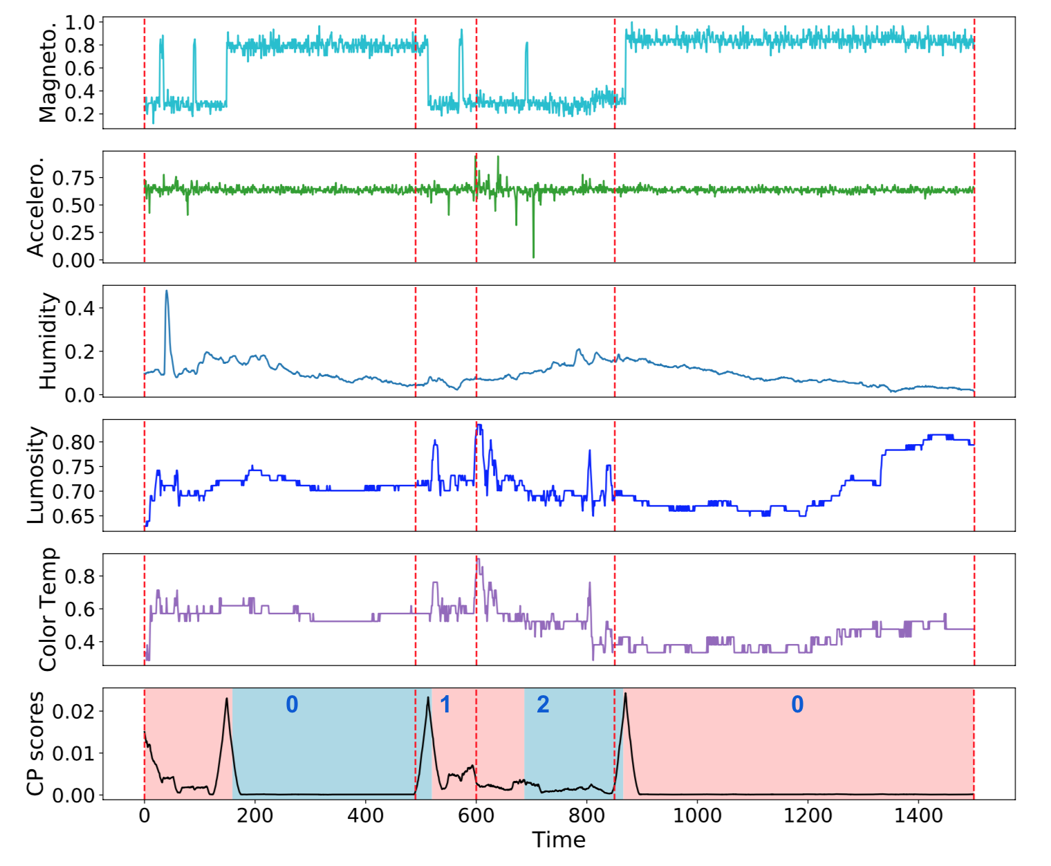
Figure 6. Performance of Cadence in an ambient sensing application. The first five plots show sensor readings obtained from different sensors. Red dashed vertical lines indicate annotations from the human labeler. The bottom plot shows change-point scores in black. Segments based on identified change point decisions are shown in alternating shaded regions of red and blue. True occupant levels in each segment are indicated in blue. We observe that there is a rough alignment between human-labeled occupancy change and change point possibility score from Cadence. A change-point score above the baseline of 0 occurs when changes are observed in raw sensor readings. Also note that there are events that are apparent from the sensor readings (around t=180), which is ignored by the occupancy annotator (absent among ground truth change points), but is apparent from change-point score.

Result. We consider the occupancy detection application where our goal is to detect the locations in the time series when the occupancy level of the room has changed based on activities captured by the sensor readings. In Figure 6, top five plots show raw readings from five selected sensors. The bottom plot shows change point scores per time-point to denote the possibility for each time-point of being a change-point using our method. The segments obtained from Cadence are shown in alternating shaded red and blue regions. We note that the change point scores above 0 correlate with sensor events and hence do not always align with human-provided occupancy change-point. Ground-truth annotations are obtained from human, which is dependent on the human perception scale about context.

Qualitatively, we observe that there is a rough alignment between human annotation of change-point and the change point score, and do not always match the peak score. One explanation for this can be events are happening in the ambient environment of that room that is ignored by the application-specific annotation (room occupancy, in this case), yet observed by sensors that can be useful for fine-grained sensing and labeling. This type of small interval events or actions may not be indicative of context-level changes such as room occupancy but can be important for in-situ sensing of interesting contextual events, partitioning, labeling, and classification in the wild (recall Partitioning step in Figure 1). Our change point detection algorithm identifies these events as change points.

Evaluation. We obtain Area under the ROC (Receiver Operating Characteristic) Curve, or AUC score, of 0.827 for our experiment to detect change points in the sensor streams from Maestro using Cadence. There are existing works that perform occupancy detection using data from ambient sensors (Ang et al., 2016; Zimmermann et al., 2018) as well as electricity consumption data from smart meter (Feng et al., 2020) in a supervised setting. To compare with existing occupancy detection systems, we use supervised occupancy detection systems using ambient sensor data based on machine learning methods such as Multilayer perceptron (MLP), Random Forest (RF), and Support Vector Machine (SVM) for performance evaluation. Our results show that Cadence, being unsupervised, provides performance (AUC: 0.827) comparable with supervised learning methods used in the literature (SVM: 0.826, MLP: 0.496, RF: 0.097). Cadence provides an easy to train, fast, unsupervised approach to identify change-points in multi-dimensional unlabeled sensor streams that can reduce human effort in partitioning time-series.

9. Experimental Evaluation

In this section, we describe details of the experimental evaluation of the proposed Cadence framework. We highlight the existing algorithms with which we compare for benchmark evaluation, the datasets used for evaluation, followed by implementation notes on our proposed framework.

9.1. Algorithms

Dataset	Application Domain	# of instances	# of CPs	% of CPs
Beedance	Biology	1057	19	1.8%
Yahoo	Network Traffic	1440	32	2.2%
HASC	Human Activity Sensing	39397	65	0.16%
Fishkiller	Environmental Science	45175	899	1.99%

Table 2. Dataset Statistics. CP indicates change-points based on annotation

We evaluate the performance of our algorithm, Cadence, with other CPD methods available in the literature for the properties mentioned in section 4.1. We select five existing methods to use to compare against Cadence. We include RDR-CPD (Liu et al., 2013), a density-ratio estimation-based method to detect changepoints using a Gaussian Kernel, and Mstats-CPD (Li et al., 2015b) using an MMD kernel for the two-sample test under the condition that a large amount of data is available. LSTNet (Lai et al., 2017) uses an RNN parameterized kernel for the kernel two-sample test. TIRE (Ryck et al., 2021) uses an autoencoder to extract time and frequency domain features and detect changepoints using euclidean distance-based dissimilarity. KL-CPD (Chang et al., 2019), the current top-performing method in the literature, uses an RNN kernel learning approach by creating additional samples when sufficient data is not available.

9.2. Dataset

We evaluate our proposed approach on 4 publicly available datasets used in change point detection literature for benchmarking. The datasets come from real-life application domains of biology, environmental science, network traffic loads, and human activity recognition. We use these datasets in our evaluation as they are the closest approximations to IoT applications that use time series partitioning, are publicly available and, are frequently used in CPD literature for benchmarking. We perform the evaluation on the following datasets:

• Bee-dance. The bee-dance dataset (bee, 2008) consists of the pixel locations in x and y dimensions and angle differences of dancer bee movements. The dance movements represent a three-stage communication method between forager bees about the orientation and distance to the food sources and water. Biologists have been interested in identifying the change point of transitioning from one stage to another of the dance and map the pattern of each stage with the information it conveys. Change point labels denote different segments (phases) of the dance in this case. Figure 7 shows a subset of the signals in the data along with predicted change point scores from the proposed method.

• Yahoo. The yahoo dataset (yah, 2017) consists of real time-series of network traffic data with anomalies, which has been manually annotated as change-points. The data consists of time-series representing metrics of various Yahoo services (e.g. CPU utilization, memory, network traffic, etc.). Change point labels here denote an abrupt rise in the incoming traffic.

• HASC. This dataset is a subset of the Human Activity Sensing Consortium (HASC) challenge 2011 dataset (has, 2011), which provides human activity information collected by portable three-axis accelerometers. The goal of change-point detection is to segment the time series data into 6 activities: stay, walk, jog, skip, stair up, and stair down. Change point labels denote the segment boundaries of the activities for this dataset.

• Fishkiller. Fishkiller dataset (Osborne et al., 2011) records sensor readings of water level from a river dam in British Columbia, Canada. When the dam does not operate normally, the water level rapidly oscillates in a short period, which leads to rapid water level drops followed by salmon fish becoming stranded and suffocating. The beginning and end of every water oscillation (the reason for fish-killing) are treated as change points and change point labels, in this case, denote abnormal functioning of the dam.

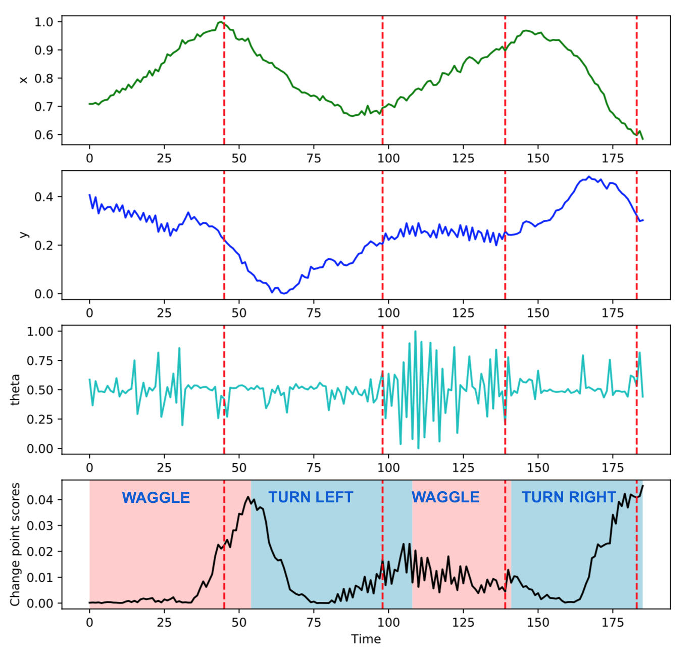
Figure 7. Predicted change point score on Beedance data using our method. In the first three plots are waggle dance signals of x, y co-ordinates, and phase angles of honey bee movement. The last plot (in black) is MMD scores obtained from our framework. Red dashed vertical lines denote ground truth change point labels (not used in prediction). Segments based on identified change point decisions are shown in alternating shaded regions of red and blue.

A summary of the data statistics is described in Table 2. We preprocess all 4 datasets by normalizing each dimension of the data in the range of [0, 1]. Note that the datasets have a varied sampling rate and are available with manual annotation of change points which we use as ground truth in evaluation. The unit of the window size is hence represented by the number of steps on the time dimension. Following (Liu et al., 2013; Saatçi, 2010; Chang et al., 2019), the datasets are divided into train-validation-test split of 60%, 20%, and 20% in chronological order.

9.3. Evaluation Metric

For the quantitative evaluation of our algorithm, we use the Receiver Operating Characteristic (ROC) curve of change point detection results as the evaluation metric. ROC curve is a plot of true positive rate (the fraction of positive examples that are correctly labeled by the classifier) against the false positive rate (the fraction of negative examples that are misclassified as positive) under different classification thresholds of the test statistic. The area under the ROC curve (AUC) is an aggregate measure of the classifier’s performance across all possible classification thresholds. While there are alternate evaluation metrics for binary classifiers such as Precision-Recall (PR) curve, ROC curve and AUC score are not biased towards classification models that perform well on the minority class at the expense of the majority class (He and Garcia, 2009; Davis and Goadrich, 2006). This is a property that is attractive when dealing with imbalanced data. Additionally, AUC is the metric commonly used in CPD literature (Chang et al., 2019; Liu et al., 2013; Li et al., 2015b) and is used as the performance metric to obtain a comparative evaluation of detection performance in this work. To calculate the AUC from the ROC curve, we obtain true positive rate and false positive rate under different change point probability thresholds, which is used to plot the ROC curve. AUC is calculated by aggregating the entire two-dimensional area under the ROC curve.

9.4. Implementation Notes

Determining the hyperparameters of the deep neural network for unsupervised learning is non-trivial. Inspired by van der Maaten et al, (Maaten and Hinton, 2008), we set the autoencoder dimensions to ${{d}-40-30-20-{z}}$ for all the datasets, where $d$ denotes the dimension of the time-series sample (data space) and $z$ denotes the dimension of latent representation (feature space). All the layers are fully connected dense layers with ReLU activation functions. We have used the same architecture and hyperparameters for all the datasets unless specifically mentioned otherwise.

We initialize the weights prior to training with Kaiming initialization for training deep neural networks with ReLU activation for better convergence (He et al., 2015). The deep autoencoder is trained for 2000 iterations without using dropout. The learning rate is set to 0.0001. We used Adam optimizer (Kingma and Ba, 2014) for all our experiments. All of the above parameters are kept fixed to achieve a reasonably low objective function value and are held constant across all datasets. Default value of $\beta=1.0$ , $w=25$ and $z=3$ are used across all datasets unless mentioned otherwise.

Note that training is fully unsupervised for our method with no information to change-point labels. We use performance on the validation set as a stopping criterion for the training procedure and select the best-parameterized model. All final results are reported based on the test set.

10. Results and Analysis

10.1. Benchmark Evaluation

In Table 3, we report the results of performance evaluation based on Area-Under-Curve (AUC) score from the ROC curve. AUC performances of existing baseline CPD techniques (except TIRE) are reported from (Chang et al., 2019).

Dataset	Beedance	Yahoo	HASC	Fishkiller
RDR-CPD	0.5197	0.6029	0.4217	0.4942
Mstats-CPD	0.5616	0.6961	0.5199	0.6392
LSTNet	0.6168	0.8863	0.5077	0.9127
TIRE	0.7001	0.7083	0.6504	0.5753
KLCPD	0.6767	0.9146	0.6490	0.9596
Cadence	0.7541	0.9774	0.6525	0.9477

Table 3. Comparative Evaluation on four datasets based on AUC score. Our method achieves best AUC in three out of the four datasets. On Fishkiller dataset it is second best by a small margin (1.2%)

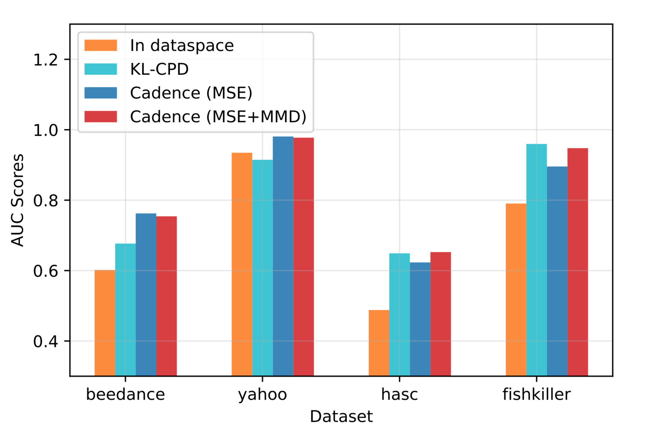
Figure 8. Ablation test of our method

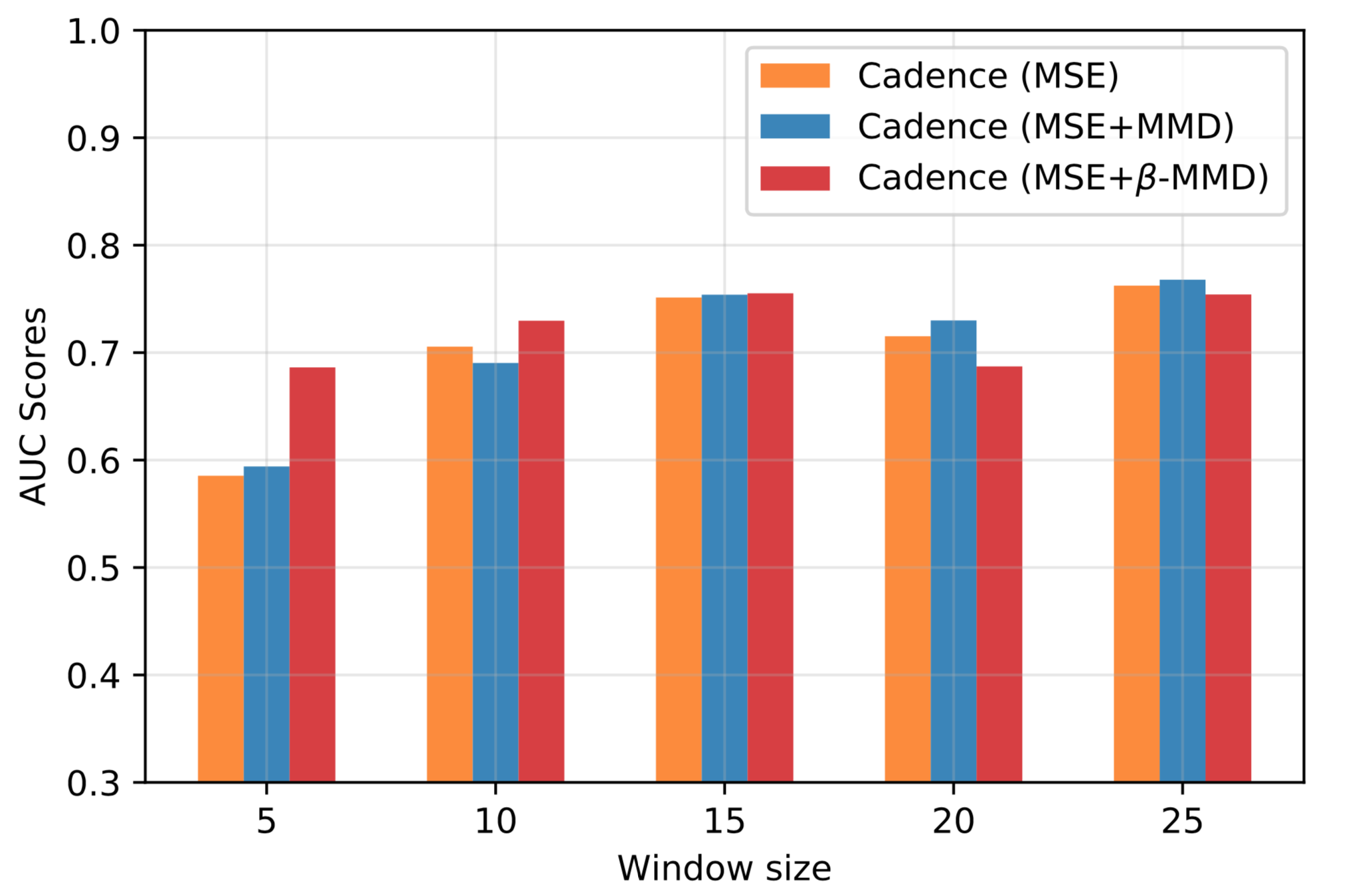
Figure 9. Ablation test for different window size

We compare with baseline methods RDR-CPD (Liu et al., 2013), which uses density-ratio estimation to detect change-points using Gaussian Kernel, and Mstats-CPD (Li et al., 2015b), which uses kernel MMD for two-sample test when a large amount of background data is available. These methods measure distribution distance using a kernel-based measure in the original data space, hence performance can be dependent on the amount of data available. LSTNet (Liu et al., 2018) uses RNN parameterized kernels for the kernel two-sample test and performs better compared to methods testing in the data space. However, for highly non-stationary and complex data (Beedance and HASC), the results are much inferior. As the changes in Yahoo and Fishkiller dataset more resembles anomaly and fault detection problem, this also shows the effectiveness of RNN-based methods in anomaly data and limitation to generalize to broader CPD problems. TIRE (Ryck et al., 2021) uses an autoencoder-based approach similar to Cadence to extract time and frequency domain features and finding change points using euclidean distance-based dissimilarity from the features. While it performs well on Beedance and HASC, on datasets such as Yahoo and Fishkiller that resemble anomaly data it performs worse due to its dependence on parameters based on domain knowledge.

KL-CPD (Chang et al., 2019), the current baseline method, uses an RNN parameterized kernel learning approach by creating additional samples to mitigate the problem of insufficient samples when sufficient data are not available. Notice that our proposed method, Cadence, shows performance comparable for both datasets (HASC and Fishkiller) where the sample size is large, but significantly outperforms KL-CPD for smaller datasets (Beedance and Yahoo). The AUC scores achieved by our method on these two datasets are 10.2% and 6.4% higher than that of KL-CPD respectively. This indicates the capability of deep autoencoders to learn meaningful, well-distinguished features through unsupervised training that is useful in performing kernel two-sample tests in the feature space.

10.2. Ablation Test on Learning Embedding

To explore how Cadence performs under different feature spaces, we perform an ablation study where our method performs kernel two-sample test with different feature mappings. To validate training a deep network for feature learning, in In dataspace the kernel-based two-sample tests are performed in the original dataspace between two segments without using a deep autoencoder. We use KL-CPD by Chang et al. (Chang et al., 2019) as a baseline method. For Cadence (MSE), kernel two-sample tests are performed on the feature space learned by optimizing reconstruction loss only. Cadence (MSE+MMD), uses maximum mean discrepancy in its objective function alongside reconstruction loss.

The results are shown in Figure 9. We observed improvement in AUC scores in all 4 datasets with up to 30% improvement over solution achieved without using a deep autoencoder (In dataspace). We further notice the generation of additional synthetic samples does offer an advantage over performing the two-sample test in data space [cyan bars rises over orange]. Cadence (MSE) [blue bars] learns the feature space without generating additional samples to balance the classes with sufficient samples. In Cadence (MSE+MMD) [red bars], our network learns more fine-grained parameterization geared towards identifying changes between segments by incorporating MMD between segments in the optimization objective. Notice that our method performs significantly better for smaller datasets (Beedance and Yahoo) than KL-CPD. We observe the advantage of adding a discrepancy measure (MMD) in the objective function for larger datasets (HASC and Fishkiller), where the composite loss function provides leverage over reconstruction loss only (red bar rises over blue bars). This validates our choice of the loss function and its advantage in our CPD goal.

Ablation Test for Window Size. We further demonstrate how Cadence performs with different optimization objectives across different window sizes, as shown in Figure 9. We trained Cadence with segments created using a sliding window, $w$ of size {5, 10, 15, 20, 25} and three versions of optimization objective: reconstruction loss only (MSE), composite loss of reconstruction plus MMD (MSE + MMD), and weighted composite loss (MSE +$\beta$-MMD). The value of $\beta$ was selected from 0.01, 0.1, 10, 100 and Cadence (MSE+MMD) is the baseline where $\beta$=1.0. Our results show that for smaller window sizes, tuning the $\beta$ parameter in Cadence-$\beta$-MMD provides leverage over the other two cases, and $\beta$=10 performs the best in such case. As the window size increases, the effect of tuning becomes negligible, and all three versions of Cadence perform similarly ($w=25$). We also see that Cadence performs better with more data (upward trend as $w$ gets larger).

We note that the two-sample test on features learned via Cadence (MSE) provides better performance over testing in the original dataspace (Figure 9). We do not observe a similar gain for Cadence (MSE + MMD) (up to 7% performance improvement above Cadence (MSE)). We make the same observation in Figure 9. Using Cadence (MSE) achieves good performance for larger window sizes. However, for small window sizes, Cadence (MSE + $\beta$-MMD) provides more robust performance.

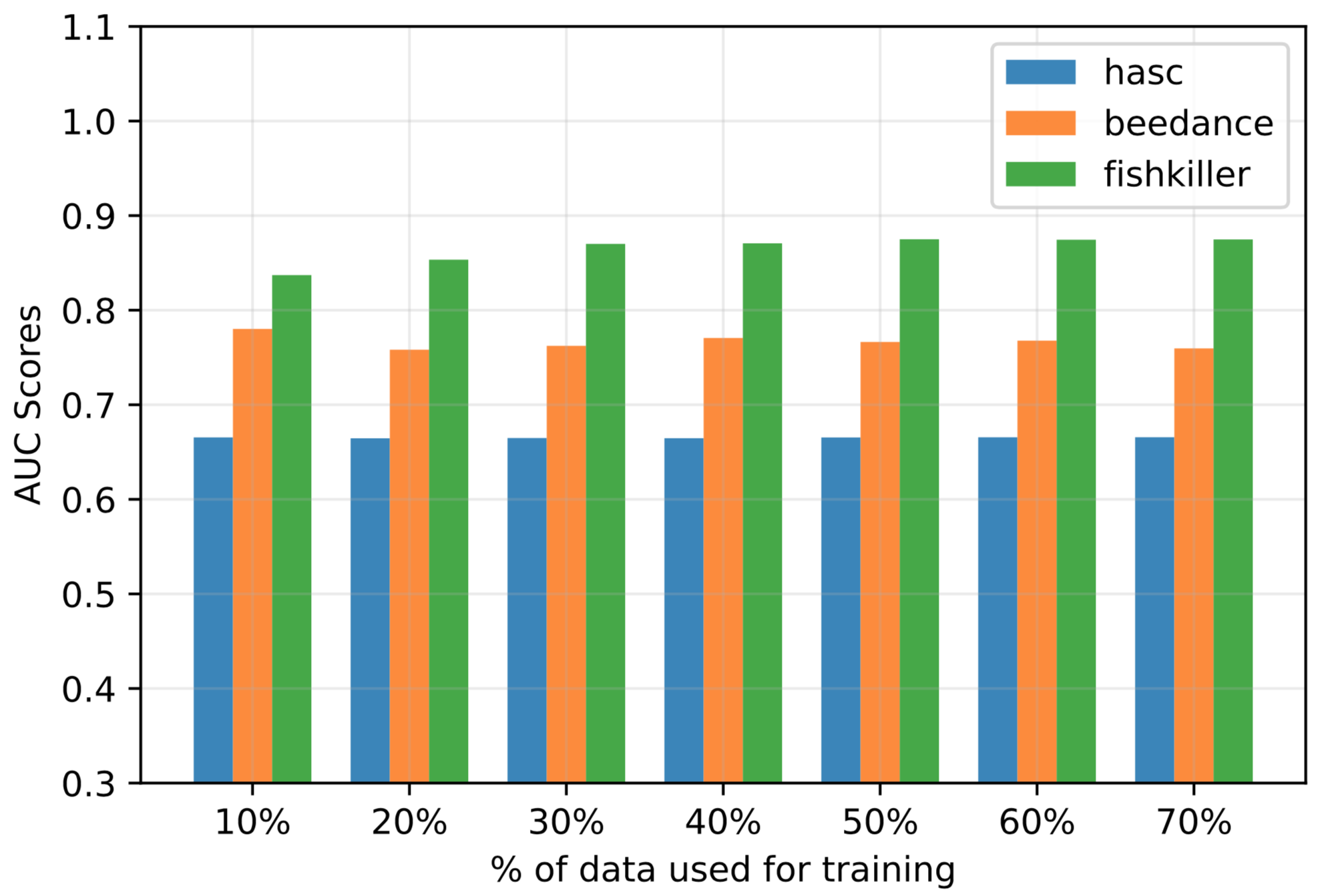
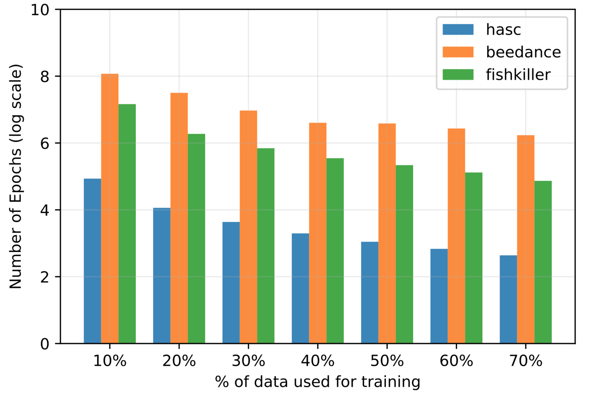
Figure 10. Our method shows stable performance under limited training data conditions as low as 10% of the available data. As the amount of training data decreases, our method still reaches the solution (left), however at the cost of more training epochs (right), which demonstrates sample efficiency of our proposed approach.

10.3. Impact of number of training samples

Recall that the amount of data available has been studied in the CPD literature as it impacts the success of kernel two-sample test based change-point detection. To demonstrate the effect of the amount of available training data on Cadence, we sample different subsets of the datasets and trained our network using fractions of training data between 10%-70% and report the achieved AUC on the test set (20%). We exclude the yahoo dataset in this experiment as its change-point labels are distributed across different fractions unevenly and thus performance on data subsets does not reflect true detection performance.

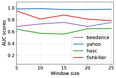
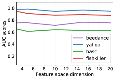
Figure 11. Effect of different window size (left) and different encoding dimension (right)

We present the results obtained in Figure  10. Cadence shows robust performance for limited training data condition as low as 10% for all three of the datasets in Figure 10 (left). This may raise concern among readers since our proposed method is unsupervised and performance deterioration is expected with less available data. However, Figure 10 (right) demonstrates that robust performance is achieved at the cost of more training time to learn the useful features for a two-sample test. Specifically, as training data decreases, Cadence still reaches the solution, however at the cost of more training epochs. In other words, Cadence leverages deep neural network parameterization to obtain useful feature mapping when training data is not sufficient. This relaxes the need for creating additional samples as suggested in (Chang et al., 2019), but the network requires more iterations to obtain that mapping when lesser data is available.

10.4. Impact of window size

Finding the right size for the sliding window is a common hyperparameter choice that can influence CPD performance. We experimented with the window size, $w$, of the segments for all 4 datasets. We varied $w$ to {5, 10, 15, 20, 25} to observe how performance varies for different window sizes. Except for Fishkiller, all three other datasets improve or provide robust performance under different window sizes in Figure 11 (left). One explanation of Fishkiller performance degradation for large window size can be the oscillatory nature of the observations. The oscillatory, seasonality pattern observed in the data, which monitors river dam functioning via sensors, can influence the MMD-based test statistic between the segments depending on the duration and frequency of the pattern.

10.5. Impact of feature space dimension

Another implementation choice for autoencoder-based optimization is the dimension of the encoded space (feature space). We study how different feature space dimensions would affect the change point detection performance of Cadence. We varied the size of the bottleneck layer of the auto-encoder, which encodes the segments in the feature space. Deep embedding learned in the lower dimension space is dependent on the size of this layer, hence it is going to influence the performance of MMD-based two-sample test statistic as well. We varied the size of this encoder layer, $z$, to {3, 5, 10, 15, 20}. We observe AUC remaining stable across these parameter settings for all four datasets in Figure 11 (right).

10.6. Impact of different kernel choices

So far we have assumed the choice of the kernel is fixed as Gaussian for all our experiments. To study the effect of kernel choices on the performance of our method, we experimented with different kernel choices from the RBF kernel family. To this end, we repeat our experiments on all 4 datasets using Gaussian (our choice of the kernel) along with Laplace and Cauchy kernels. We choose these kernels due to their positive definite properties (Fasshauer, 2011) which is fundamental to our MMD based kernel two-sample test (recall eqn. 4).

Figure 13 shows the results of our experiments. In general, we see a very small effect of kernel choice in the performance across all 4 datasets. Both Gaussian and Laplace kernel exhibit performance superior to Cauchy kernel. This suggests the suitability of RBF kernels (such as Gaussian kernel) as the dissimilarity metric for the proposed method.

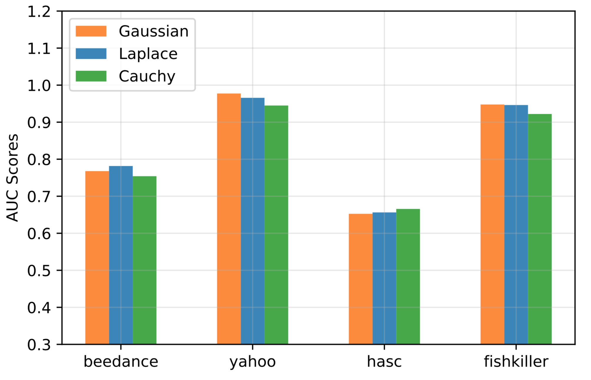
Figure 12. Effect of different kernel choice

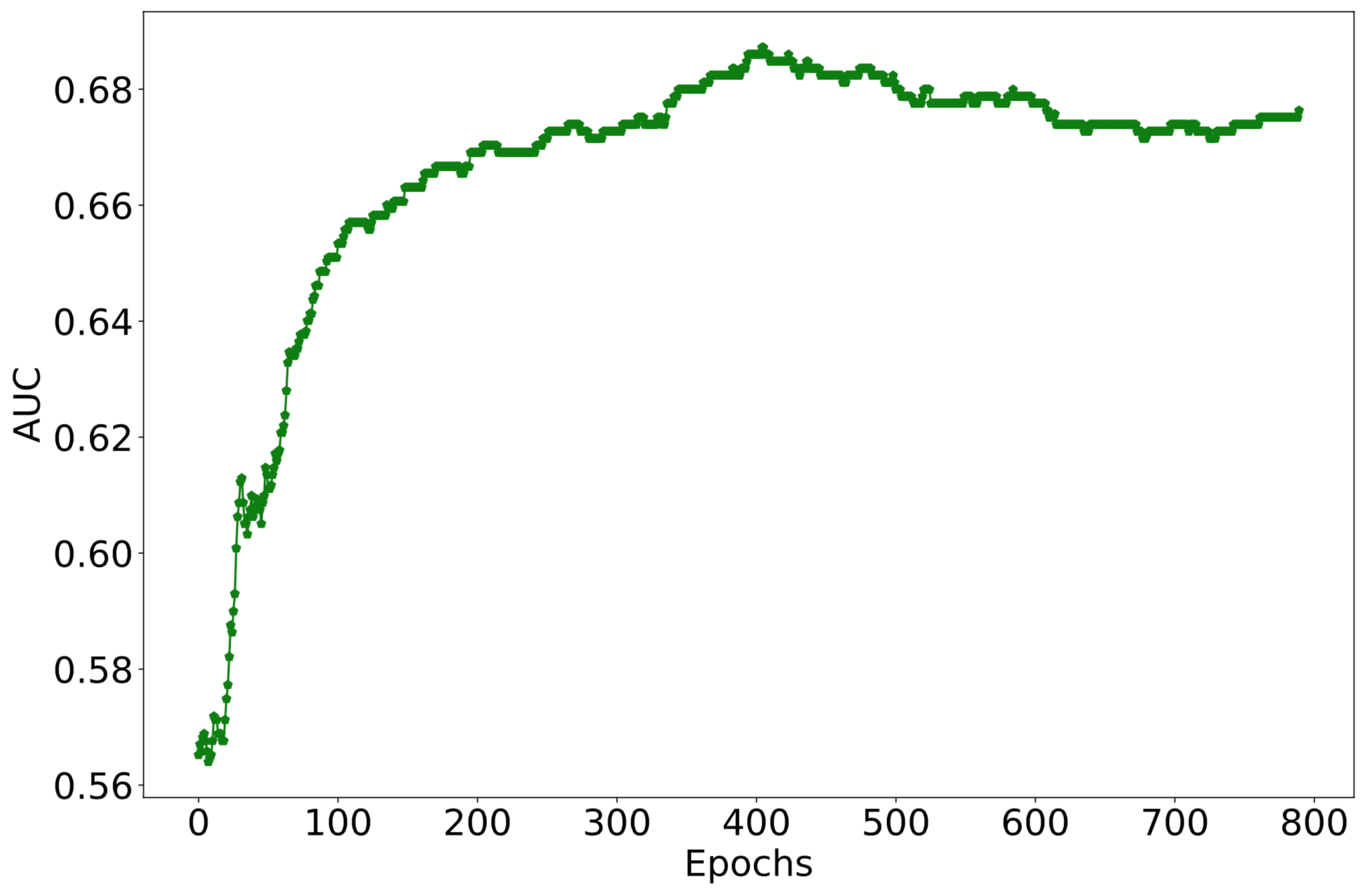
Figure 13. Performance over different epochs

10.7. Computation cost

Recall from our motivation for auto-encoder based approach for MMD-based kernel two-sample test was to obtain good performance without generating additional samples. (Chang et al., 2019) utilized a Generative Adversarial Network-based model to create additional samples for CPD problem. However, such generative models are computationally expensive and require long training time to achieve desirable performance, which can be of limited practice for deployment.

In Table 4, we present a computation complexity analysis in terms of CPU utilization, memory consumption and processing time for our method. We ran our model on a Tesla K80 machine with 12GB RAM. Processing time includes the time required for training using the best model found via early stopping criteria. We include the computational cost of KLCPD and TIRE for the purpose of comparison. For all four cases, Cadence shows the best performance in terms of CPU utilization and memory consumption (except Beedance), and processing time (except Beedance and yahoo). While TIRE also shows low CPU, memory, and time requirement because of its autoencoder-based architecture as Cadence, Cadence shows lower computation cost as it processes raw time series and has an efficient batch processing mechanism based on PyTorch. In terms of processing time, Cadence shows comparable performance to KL-CPD (in Table 4) within under 1.5 minutes whereas for hasc and fishkiller, KLCPD cannot complete processing due to computational exhaustion (denoted by Out of Memory (OOM)). Unlike KL-CPD, a generative network, Cadence relies on the autoencoder’s data compression capability in the hidden layer as a latent feature representation learning method. As a result, the model complexity and computational cost are relatively lower in comparison to other deep networks. We utilize several techniques based on the observations made in the existing literature which we believe has aided in lower computation cost while providing good performance such as the use of ReLU activation function (Livni et al., 2014) and unsupervised training for better generalization in smaller networks (Erhan et al., 2010). Datasets representative of anomaly and fault detection problems (Yahoo and Fishkiller) require less time to process due to their subtle seasonality in variation. Beedance and HASC, which capture complex distributions of biological and human activity, require longer processing time to learn the representations and perform MMD-based two-sample test. Cadence exhibits all three properties outlined in section  as we show in Table 5.

		Beedance	yahoo	hasc	fishkiller
	KLCPD	59.1	31.2	OOM	OOM
CPU Utilization (%)	TIRE	18.2	13.2	43.7	45.2
	Cadence	2.7	6.2	24.8	20.3
	KLCPD	8.3	6.4	OOM	OOM
Memory Consumption (%)	TIRE	0.5	1.8	2.3	7.2
	Cadence	1.4	0.7	1.5	0.8
	KLCPD	4570.82	21674.40	OOM	OOM
Processing Time (seconds)	TIRE	44.72	24.60	954.62	470.47
	Cadence	53.2	36.5	93	8.34

Table 4. Comparison of average CPU utilization, memory consumption, and processing time on all 4 datasets. We include KLCPD and TIRE in this comparison as they are the best performing methods. KLCPD’s CPU utilization, memory consumption, and processing time for hasc and fishkiller datasets are omitted due to computational exhaustion (OOM: Out of Memory).

11. Discussion and Future Work

Representation learning. Training of the auto-encoder is fully unsupervised in Cadence and validation performance is used as a stopping criterion. The gradual performance improvement in Figure 13 on unseen test data as training progresses implies that the training aided towards better change point detection performance on unseen data. However, following the CPD literature and prior works on MMD, we made piece-wise i.i.d assumption regarding the time series segments. Real-world datasets may not always follow this assumption. One direction for future work is to incorporate recurrent neural networks (RNN) to capture temporal dynamics in the representation learning to overcome the assumption of i.i.d samples. When data is highly non-stationary, using Variational Autoencoder (Kingma and Welling, 2013) has been explored for anomalies (Lin et al., 2020; Guo et al., 2020) and can provide leverage in better representation learning for change-point detection in future work.
Time series partitioning. Cadence uses MMD between each consecutive segment pairs as a change-point score to indicate the possibility of a given point being a change-point. However, a threshold needs to be set on MMD values to determine the location of change points in the sensor stream. In this work, we focus on finding a method that is generalizable and well-performing across various domains and Cadence shows that property using the same threshold (40% of the maximum change point score) on all the experiment datasets. However, change-point detection performance will be sensitive to the choice of threshold and further exploration for adaptive threshold choice is needed in future work.
Generalizability and Scale. Our model is developed and used in two separate phases: development (training) and inference. The training time for Cadence is dependent on the amount of data available for training. Training from scratch may require a large dataset and increased training time. However, this can be reduced with transfer learning (Zhuang et al., 2020; Liu et al., 2019) where a previously trained model can be trained with much fewer iterations using new data and pre-trained weights. In the inference phase, the trained model can be applied to streaming data in batches and can thus scale to large data. The inference-generation throughput may be a bottleneck for large-scale streaming applications. Cadence’s inference time is $\sim{30}$ milliseconds (KLCPD: $\sim{4.45}$ seconds, TIRE: $\sim{225}$ milliseconds) which should cover a large class of IoT applications. However, we leave related scaling challenges for massive streaming applications for future work.

Algorithms	Ease of use	Computational Efficiency	Performance
RDR-CPD (Liu et al., 2013)	✓	✗	✗
Mstats-CPD (Li et al., 2015b)	✗	✓	✗
LSTNet (Liu et al., 2018)	✓	✗	✗
TIRE(Ryck et al., 2021)	✓	✓	✗
KLCPD (Chang et al., 2019)	✗	✗	✓
Cadence (Proposed Approach)	✓	✓	✓

Table 5. Overview of properties exhibited by existing CPD algorithms. We design our proposed approach, Cadence, to exhibit all three properties.

12. Conclusion

This paper presents Cadence - a framework that projects a set of time series samples in a jointly optimized feature space towards change-point detection. It works by iteratively optimizing a custom representation learning objective based on the discrepancy between time-series samples. Using this novel feature mapping, our approach provides a way to detect time-series events without using change-point labels provided by a human. We evaluate our proposed algorithm, Cadence, with public change point detection datasets and present its performance for different parameter settings in the paper. We compared Cadence’s performance with the state-of-the-art techniques and showed its superior performance as well as robustness to hyperparameter tuning and sample efficiency. Its good performance is obtained within surprisingly less time, with a simpler, easy to train, and generalizable model. With these properties, Cadence has the potential to scale well for practical deployment in applications of general-purpose sensing and continuous learning without human input.

References

- (1)
- bee (2008) 2008. Honey Bee Waggle Data. https://www.cc.gatech.edu/~borg/ijcv_psslds/
- has (2011) 2011. HASC 2011 Data. http://hasc.jp/hc2011/
- yah (2017) 2017. Yahoo Web Data. https://webscope.sandbox.yahoo.com
- Abedin et al. (2021) Alireza Abedin, Mahsa Ehsanpour, Qinfeng Shi, Hamid Rezatofighi, and Damith C. Ranasinghe. 2021. Attend and Discriminate: Beyond the State-of-the-Art for Human Activity Recognition Using Wearable Sensors. Proc. ACM Interact. Mob. Wearable Ubiquitous Technol. 5, 1, Article 1 (March 2021), 22 pages. https://doi.org/10.1145/3448083
- Adams and Mackay (2007) Ryan P. Adams and David J.C. Mackay. 2007. Bayesian Online Changepoint Detection.
- Adams and MacKay (2007) Ryan Prescott Adams and David JC MacKay. 2007. Bayesian online changepoint detection. arXiv preprint arXiv:0710.3742 (2007).
- Aminikhanghahi and Cook (2017) S. Aminikhanghahi and D. J. Cook. 2017. A Survey of Methods for Time Series Change Point Detection. Knowledge and information systems 51, 2 (May 2017), 339–367.
- Aminikhanghahi and Cook (2017) S. Aminikhanghahi and D. J. Cook. 2017. Using change point detection to automate daily activity segmentation. In 2017 IEEE International Conference on Pervasive Computing and Communications Workshops. 262–267.
- Aminikhanghahi and Cook (2017) Samaneh Aminikhanghahi and Diane J Cook. 2017. Using change point detection to automate daily activity segmentation. In 2017 IEEE International Conference on Pervasive Computing and Communications Workshops (PerCom Workshops). IEEE, 262–267.
- Aminikhanghahi et al. (2018) Samaneh Aminikhanghahi, Tinghui Wang, and Diane J Cook. 2018. Real-time change point detection with application to smart home time series data. IEEE Transactions on Knowledge and Data Engineering 31, 5 (2018), 1010–1023.
- Ang et al. (2016) Irvan Bastian Arief Ang, Flora Dilys Salim, and Margaret Hamilton. 2016. Human occupancy recognition with multivariate ambient sensors. In 2016 IEEE International Conference on Pervasive Computing and Communication Workshops (PerCom Workshops). 1–6. https://doi.org/10.1109/PERCOMW.2016.7457116
- Atzori et al. (2010) L. Atzori, A. Iera, and G. Morabito. 2010. The Internet of Things: A survey. Computer Networks 54, 15 (Oct. 2010), 2787–2805.
- Bai et al. (2020) Lei Bai, Lina Yao, Xianzhi Wang, Salil S. Kanhere, Bin Guo, and Zhiwen Yu. 2020. Adversarial Multi-View Networks for Activity Recognition. Proc. ACM Interact. Mob. Wearable Ubiquitous Technol. 4, 2, Article 42 (June 2020), 22 pages. https://doi.org/10.1145/3397323
- Banerjee and Guhathakurta (2020) Sayantan Banerjee and Kousik Guhathakurta. 2020. Change‐point analysis in financial networks. Stat 9, 1 (Jan 2020).
- Basseville and Nikiforov (1993) Michèle Basseville and Igor V. Nikiforov. 1993. Detection of Abrupt Changes: Theory and Application. Prentice-Hall, Inc., Upper Saddle River, NJ, USA.
- Bonacina et al. (2020) Fabrizio Bonacina, Eric Stefan Miele, and Alessandro Corsini. 2020. Time Series Clustering: A Complex Network-Based Approach for Feature Selection in Multi-Sensor Data. Modelling 1, 1 (2020), 1–21. https://doi.org/10.3390/modelling1010001
- Chang et al. (2019) Wei-Cheng Chang, Chun-Liang Li, Yiming Yang, and Barnabás Póczos. 2019. Kernel Change-point Detection with Auxiliary Deep Generative Models. In International Conference on Learning Representations.
- Chowdhury et al. (2012) Md Foezur Rahman Chowdhury, Sid-Ahmed Selouani, and Douglas D. O’Shaughnessy. 2012. A highly non-stationary noise tracking and compensation algorithm, with applications to speech enhancement and on-line ASR. 2012 IEEE International Conference on Acoustics, Speech and Signal Processing (ICASSP) (2012), 4337–4340.
- Chung et al. (2015) Junyoung Chung, Kyle Kastner, Laurent Dinh, Kratarth Goel, Aaron Courville, and Yoshua Bengio. 2015. A recurrent latent variable model for sequential data. arXiv preprint arXiv:1506.02216 (2015).
- Davis and Goadrich (2006) Jesse Davis and Mark Goadrich. 2006. The relationship between Precision-Recall and ROC curves. In Proceedings of the 23rd international conference on Machine learning. 233–240.
- De Ryck et al. (2020) Tim De Ryck, Maarten De Vos, and Alexander Bertrand. 2020. Change Point Detection in Time Series Data using Autoencoders with a Time-Invariant Representation. arXiv preprint arXiv:2008.09524 (2020).
- Erhan et al. (2010) Dumitru Erhan, Aaron Courville, Yoshua Bengio, and Pascal Vincent. 2010. Why does unsupervised pre-training help deep learning?. In Proceedings of the thirteenth international conference on artificial intelligence and statistics. JMLR Workshop and Conference Proceedings, 201–208.
- Fasshauer (2011) G. E. Fasshauer. 2011. Positive definite kernels: past, present and future. (2011).
- Feng et al. (2020) Cong Feng, Ali Mehmani, and Jie Zhang. 2020. Deep Learning-Based Real-Time Building Occupancy Detection Using AMI Data. IEEE Transactions on Smart Grid 11, 5 (2020), 4490–4501. https://doi.org/10.1109/TSG.2020.2982351
- Greenwald and Oertel (2017) Hal S. Greenwald and Carsten K. Oertel. 2017. Future Directions in Machine Learning. Frontiers in Robotics and AI 3 (2017), 79.
- Gretton et al. (2012a) Arthur Gretton, Karsten M Borgwardt, Malte J Rasch, Bernhard Schölkopf, and Alexander Smola. 2012a. A kernel two-sample test. Journal of Machine Learning Research 13, Mar (2012), 723–773.
- Gretton et al. (2009) Arthur Gretton, Kenji Fukumizu, Zaïd Harchaoui, and Bharath K. Sriperumbudur. 2009. A Fast, Consistent Kernel Two-Sample Test. In Advances in Neural Information Processing Systems 22. 673–681.
- Gretton et al. (2012b) A. Gretton, D. Sejdinovic, H. Strathmann, S. Balakrishnan, M. Pontil, K. Fukumizu, and B. K Sriperumbudur. 2012b. Optimal kernel choice for large-scale two-sample tests. In Advances in neural information processing systems. 1205–1213.
- Gubbia et al. (2013) J. Gubbia, R. Buyya, S. Marusic, and M. Palaniswami. 2013. Internet of Things (IoT): A vision, architectural elements, and future directions. Future Generation Computer Systems 29, 7 (Sept. 2013), 1645–1660.
- Guo et al. (2018) Xiaonan Guo, Jian Liu, Cong Shi, Hongbo Liu, Yingying Chen, and Mooi Choo Chuah. 2018. Device-free personalized fitness assistant using WiFi. Proceedings of the ACM on Interactive, Mobile, Wearable and Ubiquitous Technologies 2, 4 (2018), 1–23.
- Guo et al. (2020) Yifan Guo, Tianxi Ji, Qianlong Wang, Lixing Yu, Geyong Min, and Pan Li. 2020. Unsupervised Anomaly Detection in IoT Systems for Smart Cities. IEEE Transactions on Network Science and Engineering 7, 4 (2020), 2231–2242. https://doi.org/10.1109/TNSE.2020.3027543
- Gustafsson (1996) F. Gustafsson. 1996. The marginalized likelihood ratio test for detecting abrupt changes. IEEE Trans. Automat. Control 41, 1 (1996), 66–78.
- Harchaoui et al. (2008) Zaïd Harchaoui, Francis Bach, and Éric Moulines. 2008. Kernel Change-Point Analysis. In 21st International Conference on Neural Information Processing Systems (NIPS’08). 609–616.
- Härdle et al. (2004) W. Härdle, A. Werwatz, M. Müller, and S. Sperlich. 2004. Nonparametric density estimation. In Nonparametric and semiparametric models. 39–83.
- He and Garcia (2009) Haibo He and Edwardo A Garcia. 2009. Learning from imbalanced data. IEEE Transactions on knowledge and data engineering 21, 9 (2009), 1263–1284.
- He et al. (2015) Kaiming He, Xiangyu Zhang, Shaoqing Ren, and Jian Sun. 2015. Delving deep into rectifiers: Surpassing human-level performance on imagenet classification. In Proceedings of the IEEE international conference on computer vision. 1026–1034.
- Hinton and Salakhutdinov (2006) Geoffrey E Hinton and Ruslan R Salakhutdinov. 2006. Reducing the dimensionality of data with neural networks. science 313, 5786 (2006), 504–507.
- Huang et al. (2019) Anna Huang, Dong Wang, Run Zhao, and Qian Zhang. 2019. Au-Id: Automatic User Identification and Authentication through the Motions Captured from Sequential Human Activities Using RFID. Proc. ACM Interact. Mob. Wearable Ubiquitous Technol. 3, 2, Article 48 (June 2019), 26 pages. https://doi.org/10.1145/3328919
- Huynh et al. (2019) Sinh Huynh, Rajesh Krishna Balan, JeongGil Ko, and Youngki Lee. 2019. VitaMon: Measuring Heart Rate Variability Using Smartphone Front Camera. In 17th Conference on Embedded Networked Sensor Systems (SenSys ’19). 1–14.
- Idé and Tsuda (2007) Tsuyoshi Idé and Koji Tsuda. 2007. Change-Point Detection using Krylov Subspace Learning. In Proceedings of the Seventh SIAM International Conference on Data Mining, April 26-28, 2007, Minneapolis, Minnesota, USA. 515–520.
- Janardan and Mehta (2017) Janardan and Shikha Mehta. 2017. Concept drift in Streaming Data Classification: Algorithms, Platforms and Issues. 122 (2017), 804 – 811. 5th International Conference on Information Technology and Quantitative Management, ITQM 2017.
- Jeyakumar et al. (2019) Jeya Vikranth Jeyakumar, Liangzhen Lai, Naveen Suda, and Mani Srivastava. 2019. SenseHAR: A Robust Virtual Activity Sensor for Smartphones and Wearables. In 17th Conference on Embedded Networked Sensor Systems (SenSys ’19). 15–28.
- Kanamori et al. (2009) T. Kanamori, S. Hido, and M. Sugiyama. 2009. A least-squares approach to direct importance estimation. Journal of Machine Learning Research 10, Jul (2009), 1391–1445.
- Kawahara et al. (2007) Y. Kawahara, T. Yairi, and K. Machida. 2007. Change-Point Detection using Krylov Subspace Learning. In Proceedings of the Seventh IEEE International Conference on Data Mining, 2007. 559–564.
- Keogh et al. (2004) Eamonn Keogh, Selina Chu, David Hart, and Michael Pazzani. 2004. Segmenting time series: A survey and novel approach. In Data mining in time series databases. World Scientific, 1–21.
- Keogh and Lin (2005) Eamonn Keogh and Jessica Lin. 2005. Clustering of time-series subsequences is meaningless: implications for previous and future research. Knowledge and information systems 8, 2 (2005), 154–177.
- Kingma and Ba (2014) Diederik P Kingma and Jimmy Ba. 2014. Adam: A method for stochastic optimization. arXiv preprint arXiv:1412.6980 (2014).
- Kingma and Welling (2013) Diederik P Kingma and Max Welling. 2013. Auto-encoding variational bayes. arXiv preprint arXiv:1312.6114 (2013).
- Kwon et al. (2020) Hyeokhyen Kwon, Catherine Tong, Harish Haresamudram, Yan Gao, Gregory D. Abowd, Nicholas D. Lane, and Thomas Plötz. 2020. IMUTube: Automatic Extraction of Virtual on-Body Accelerometry from Video for Human Activity Recognition. Proc. ACM Interact. Mob. Wearable Ubiquitous Technol. 4, 3, Article 87 (Sept. 2020), 29 pages. https://doi.org/10.1145/3411841
- Lai et al. (2017) Guokun Lai, Wei-Cheng Chang, Yiming Yang, and Hanxiao Liu. 2017. Modeling Long- and Short-Term Temporal Patterns with Deep Neural Networks. CoRR abs/1703.07015 (2017). http://arxiv.org/abs/1703.07015
- Le (2013) Quoc V Le. 2013. Building high-level features using large scale unsupervised learning. In 2013 IEEE international conference on acoustics, speech and signal processing. IEEE, 8595–8598.
- LeCun et al. (2015) Yann LeCun, Yoshua Bengio, and Geoffrey Hinton. 2015. Deep learning. nature 521, 7553 (2015), 436–444.
- Lee et al. (2018) Wei-Han Lee, Jorge Ortiz, Bongjun Ko, and Ruby Lee. 2018. Time series segmentation through automatic feature learning. arXiv preprint arXiv:1801.05394 (2018).
- Li et al. (2015a) S. Li, Y. Xie, H. Dai, and L. Song. 2015a. M-Statistic for Kernel Change-Point Detection. In Advances in Neural Information Processing Systems 28. 3366–3374.
- Li et al. (2015b) Shuang Li, Yao Xie, Hanjun Dai, and Le Song. 2015b. M-Statistic for Kernel Change-Point Detection. In 28th International Conference on Neural Information Processing Systems (NIPS’15, Vol. 2). 3366–3374.
- Li ([n.d.]) Wei Z. Jia W. Sun M. Li, Z. [n.d.]. Daily life event segmentation for lifestyle evaluation based on multi-sensor data recorded by a wearable device. ([n. d.]).
- Lin et al. (2020) S. Lin, R. Clark, R. Birke, S. Schönborn, N. Trigoni, and S. Roberts. 2020. Anomaly Detection for Time Series Using VAE-LSTM Hybrid Model. In ICASSP 2020 - 2020 IEEE International Conference on Acoustics, Speech and Signal Processing (ICASSP). 4322–4326. https://doi.org/10.1109/ICASSP40776.2020.9053558
- Liu et al. (2013) Song Liu, Makoto Yamada, Nigel Collier, and Masashi Sugiyama. 2013. Change-point detection in time-series data by relative density-ratio estimation. Neural Networks 43 (2013), 72–83.
- Liu et al. (2019) Tong Liu, Shakeel Alibhai, Jinzhen Wang, Qing Liu, Xubin He, and Chentao Wu. 2019. Exploring Transfer Learning to Reduce Training Overhead of HPC Data in Machine Learning. In 2019 IEEE International Conference on Networking, Architecture and Storage (NAS). 1–7. https://doi.org/10.1109/NAS.2019.8834723
- Liu et al. ([n.d.]) T. Y. Liu, T. Qin, B. Shao, W. Chen, and J. Bian. [n.d.]. Machine Learning: Research hotspots in the next ten years. https://www.microsoft.com/en-us/research/lab/microsoft-research-asia/articles/machine-learning-research-hotspots/.
- Liu et al. (2018) Yusha Liu, Chun-Liang Li, and Barnabás Póczos. 2018. Classifier Two Sample Test for Video Anomaly Detections. In BMVC.
- Livni et al. (2014) Roi Livni, Shai Shalev-Shwartz, and Ohad Shamir. 2014. On the Computational Efficiency of Training Neural Networks. In Proceedings of the 27th International Conference on Neural Information Processing Systems - Volume 1 (Montreal, Canada) (NIPS’14). MIT Press, Cambridge, MA, USA, 855–863.
- Lowry et al. (1992) Cynthia A. Lowry, William H. Woodall, Charles W. Champ, and Steven E. Rigdon. 1992. A multivariate exponentially weighted moving average control chart.
- Ma et al. (2021) Haojie Ma, Zhijie Zhang, Wenzhong Li, and Sanglu Lu. 2021. Unsupervised Human Activity Representation Learning with Multi-Task Deep Clustering. Proc. ACM Interact. Mob. Wearable Ubiquitous Technol. 5, 1, Article 48 (March 2021), 25 pages. https://doi.org/10.1145/3448074
- Maaten and Hinton (2008) Laurens van der Maaten and Geoffrey Hinton. 2008. Visualizing data using t-SNE. Journal of machine learning research 9, Nov (2008), 2579–2605.
- Moskvina and Zhigljavsky (2003) V. Moskvina and A. Zhigljavsky. 2003. An Algorithm Based on Singular Spectrum Analysis for Change-Point Detection. Communications in Statistics-simulation and Computation 32 (01 2003), 319–352.
- Nassar et al. (2010) Matthew R. Nassar, Robert C. Wilson, Benjamin S. Heasly, and Joshua I. Gold. 2010. An approximately Bayesian delta-rule model explains the dynamics of belief updating in a changing environment. The Journal of neuroscience : the official journal of the Society for Neuroscience 30, 37 (2010), 12366–78.
- Nguyen et al. (2019) Viet Nguyen, Siddharth Rupavatharam, Luyang Liu, Richard Howard, and Marco Gruteser. 2019. HandSense: Capacitive Coupling-Based Dynamic, Micro Finger Gesture Recognition. In Proceedings of the 17th Conference on Embedded Networked Sensor Systems (SenSys ’19). 285–297.
- Ni et al. (2018) Qin Ni, Lei Zhang, and Luqun Li. 2018. A Heterogeneous Ensemble Approach for Activity Recognition with Integration of Change Point-Based Data Segmentation. Applied Sciences 8, 9 (2018), 1695.
- Nishiyama and Fukumizu (2016) Yu Nishiyama and Kenji Fukumizu. 2016. Characteristic kernels and infinitely divisible distributions. The Journal of Machine Learning Research 17, 1 (2016), 6240–6267.
- Noor et al. (2017) Mohd Halim Mohd Noor, Zoran Salcic, I Kevin, and Kai Wang. 2017. Adaptive sliding window segmentation for physical activity recognition using a single tri-axial accelerometer. Pervasive and Mobile Computing 38 (2017), 41–59.
- Ohara et al. (2017) Kazuya Ohara, Takuya Maekawa, and Yasuyuki Matsushita. 2017. Detecting State Changes of Indoor Everyday Objects Using Wi-Fi Channel State Information. Proc. ACM Interact. Mob. Wearable Ubiquitous Technol. 1, 3, Article 88 (Sept. 2017), 28 pages. https://doi.org/10.1145/3131898
- Osborne et al. (2011) Michael Osborne, Roman Garnett, Kevin Swersky, and Nando De Freitas. 2011. A machine learning approach to pattern detection and prediction for environmental monitoring and water sustainability. In ICML Workshop on Machine Learning for Global Challenges.
- Pan et al. (2019) Shijia Pan, Mario Berges, Juleen Rodakowski, Pei Zhang, and Hae Young Noh. 2019. Fine-grained recognition of activities of daily living through structural vibration and electrical sensing. In 6th ACM International Conference on Systems for Energy-Efficient Buildings, Cities, and Transportation. 149–158.
- Pérez-Cruz (2008) Fernando Pérez-Cruz. 2008. Kullback-Leibler divergence estimation of continuous distributions. In 2008 IEEE international symposium on information theory. IEEE, 1666–1670.
- Ramdas et al. (2015) A. Ramdas, S. J. Reddi, B. Póczos, A. Singh, and L. Wasserman. 2015. On the decreasing power of kernel and distance based nonparametric hypothesis tests in high dimensions. In Twenty-Ninth AAAI Conference on Artificial Intelligence.
- Ryck et al. (2021) Tim De Ryck, Maarten De Vos, and Alexander Bertrand. 2021. Change Point Detection in Time Series Data using Autoencoders with a Time-Invariant Representation. arXiv:2008.09524 [cs.LG]
- Saatçi et al. (2010) Yunus Saatçi, Ryan Turner, and Carl Edward Rasmussen. 2010. Gaussian Process Change Point Models. In Proceedings of the 27th International Conference on International Conference on Machine Learning (ICML’10). 927–934.
- Saatçi (2010) Yunus Saatçi. 2010. Gaussian Process Change Point Models.
- Sadri et al. (2018) Amin Sadri, Flora D. Salim, Yongli Ren, Wei Shao, John C. Krumm, and Cecilia Mascolo. 2018. What Will You Do for the Rest of the Day? An Approach to Continuous Trajectory Prediction. Proc. ACM Interact. Mob. Wearable Ubiquitous Technol. 2, 4, Article 186 (Dec. 2018), 26 pages. https://doi.org/10.1145/3287064
- Saeed et al. (2021) Aaqib Saeed, Flora D. Salim, Tanir Ozcelebi, and Johan Lukkien. 2021. Federated Self-Supervised Learning of Multisensor Representations for Embedded Intelligence. IEEE Internet of Things Journal 8, 2 (Jan 2021), 1030–1040. https://doi.org/10.1109/jiot.2020.3009358
- Sarker et al. (2018) Iqbal H Sarker, Alan Colman, Muhammad Ashad Kabir, and Jun Han. 2018. Individualized time-series segmentation for mining mobile phone user behavior. Comput. J. 61, 3 (2018), 349–368.
- Schölkopf et al. (2002) Bernhard Schölkopf, Alexander J Smola, Francis Bach, et al. 2002. Learning with kernels: support vector machines, regularization, optimization, and beyond.
- Sinn et al. (2012) Mathieu Sinn, Ali Ghodsi, and Karsten Keller. 2012. Detecting change-points in time series by maximum mean discrepancy of ordinal pattern distributions. In Proceedings of the Twenty-Eighth Conference on Uncertainty in Artificial Intelligence. 786–794.
- Stankovic (2014) J. Stankovic. 2014. Research Directions for the Internet of Things. IEEE Internet of Things Journal 1, 1 (Feb. 2014), 3 – 9.
- Sugiyama et al. (2008) M. Sugiyama, S. Nakajima, H. Kashima, P. V. Buenau, and M. Kawanabe. 2008. Direct importance estimation with model selection and its application to covariate shift adaptation. In Advances in neural information processing systems. 1433–1440.
- Sugiyama et al. (2012) M. Sugiyama, T. Suzuki, and T. Kanamori. 2012. Density ratio estimation in machine learning. Cambridge University Press.
- Takayasu (2015) H. Takayasu. 2015. Basic methods of change-point detection of financial fluctuations. In 2015 International Conference on Noise and Fluctuations (ICNF). 1–3.
- Tang et al. (2021) Chi Ian Tang, Ignacio Perez-Pozuelo, Dimitris Spathis, Soren Brage, Nick Wareham, and Cecilia Mascolo. 2021. SelfHAR: Improving Human Activity Recognition through Self-Training with Unlabeled Data. Proc. ACM Interact. Mob. Wearable Ubiquitous Technol. 5, 1, Article 36 (March 2021), 30 pages. https://doi.org/10.1145/3448112
- Vincent et al. (2010) P. Vincent, H. Larochelle, I. Lajoie, Y. Bengio, and P. A. Manzagol. 2010. Stacked denoising autoencoders: Learning useful representations in a deep network with a local denoising criterion. Journal of machine learning research 11, Dec (2010), 3371–3408.
- Wang et al. (2019) Chongyang Wang, Temitayo A. Olugbade, Akhil Mathur, Amanda C. De C. Williams, Nicholas D. Lane, and Nadia Bianchi-Berthouze. 2019. Recurrent Network Based Automatic Detection of Chronic Pain Protective Behavior Using MoCap and SEMG Data. In Proceedings of the 23rd International Symposium on Wearable Computers (ISWC ’19). 225–230.
- Wang et al. (2011) Y. Wang, C. Wu, Z. Ji, B. Wang, and Y. Liang. 2011. Non-Parametric Change-Point Method for Differential Gene Expression Detection. PloS one 6 (05 2011), e20060.
- Wang and Zheng (2018) Yanwen Wang and Yuanqing Zheng. 2018. Modeling RFID Signal Reflection for Contact-Free Activity Recognition. Proc. ACM Interact. Mob. Wearable Ubiquitous Technol. 2, 4, Article 193 (Dec. 2018), 22 pages. https://doi.org/10.1145/3287071
- Webb et al. (2016) G. I. Webb, R. Hyde, H. Cao, H. L. Nguyen, and F. Petitjean. 2016. Characterizing Concept Drift. Data Min. Knowl. Discov. 30, 4 (2016), 964–994.
- Willsky and Jones (1976) A. Willsky and H. Jones. 1976. A generalized likelihood ratio approach to the detection and estimation of jumps in linear systems. IEEE Trans. Automat. Control 21, 1 (1976), 108–112.
- Yamanishi et al. (2000) K. Yamanishi, J. Takeuchi, G. Williams, and P. Milne. 2000. On-Line Unsupervised Outlier Detection Using Finite Mixtures with Discounting Learning Algorithms. In 6th International Conference on Knowledge Discovery and Data Mining (KDD ’00). 320–324.
- Yamanishi and Takeuchi (2002) Kenji Yamanishi and Jun-ichi Takeuchi. 2002. A Unifying Framework for Detecting Outliers and Change Points from Non-Stationary Time Series Data. In Proceedings of the Eighth ACM SIGKDD International Conference on Knowledge Discovery and Data Mining (KDD ’02). 676–681.
- Zhang et al. (2020) Ruohong Zhang, Yu Hao, Donghan Yu, Wei-Cheng Chang, Guokun Lai, and Yiming Yang. 2020. Explainable Unsupervised Change-point Detection via Graph Neural Networks. arXiv:2004.11934 [cs.LG]
- Zhuang et al. (2020) Fuzhen Zhuang, Zhiyuan Qi, Keyu Duan, Dongbo Xi, Yongchun Zhu, Hengshu Zhu, Hui Xiong, and Qing He. 2020. A Comprehensive Survey on Transfer Learning. arXiv:1911.02685 [cs.LG]
- Zimmermann et al. (2018) Lars Zimmermann, Robert Weigel, and Georg Fischer. 2018. Fusion of Nonintrusive Environmental Sensors for Occupancy Detection in Smart Homes. IEEE Internet of Things Journal 5, 4 (2018), 2343–2352. https://doi.org/10.1109/JIOT.2017.2752134
- Zou et al. (2014) Shaofeng Zou, Yingbin Liang, H. Vincent Poor, and Xinghua Mindy Shi. 2014. Nonparametric Detection of Anomalous Data via Kernel Mean Embedding. (04 2014).