Multidimensional Assignment Problem for multipartite entity resolution

Abstract

Multipartite entity resolution aims at integrating records from multiple datasets into one entity. We derive a mathematical formulation for a general class of record linkage problems in multipartite entity resolution across many datasets as a combinatorial optimization problem known as the multidimensional assignment problem. As a motivation for our approach, we illustrate the advantage of multipartite entity resolution over sequential bipartite matching. Because the optimization problem is NP-hard, we apply two heuristic procedures, a Greedy algorithm and very large scale neighborhood search, to solve the assignment problem and find the most likely matching of records from multiple datasets into a single entity. We evaluate and compare the performance of these algorithms and their modifications on synthetically generated data. We perform computational experiments to compare performance of recent heuristic, the very large-scale neighborhood search, with a Greedy algorithm, another heuristic for the MAP, as well as with two versions of genetic algorithm, a general metaheuristic. Importantly, we perform experiments to compare two alternative methods of re-starting the search for the former heuristic, specifically a random-sampling multi-start and a deterministic design-based multi-start. We find evidence that design-based multi-start can be more efficient as the size of databases grow large. In addition, we show that very large scale search, especially its multi-start version, outperforms simple Greedy heuristic. Hybridization of Greedy search with very large scale neighborhood search improves the performance. Using multi-start with as few as three additional runs of very large scale search offers some improvement in the performance of the very large scale search procedure. Last, we propose an approach to evaluating complexity of the very large-scale neighborhood search.

1 Introduction

In this paper, we describe a computationally challenging new application of the multidimensional assignment problem (MAP). We show how this application of the MAP arises naturally when simultaneously merging multiple massive datasets. Because finding global optimum for large-size instances of the MAP remains a significant hurdle, we apply a recent metaheuristic approach, known as the very large-scale neighborhood search (VLSNS), for solving the MAPs. Due to its novelty, the VLSNS algorithm is much less studied than other approaches for the MAP. In particular, it has not been evaluated on larger-sized problem instances, with exception of limited computational experiment in kammerdiner2017very . Therefore, we conduct extensive numerical experiments aimed at comparison of this solution method with state-of-the-art Greedy algorithm and with the global optimal solutions given by a standard linear solver such as Gurobi. We find that this novel metaheuristic shows good performance in our numerical comparison, and therefore, can be used in the context of merging multiple datasets known as multipartite entity resolution.

The amount of the information on the Internet increases every year. In 2005 there were 150 exabytes digital information produced; and there were already 1200 exabytes in 2010 Helbing2011 . Nearly 70% of this content is user generated ijwet2013 . One of the enablers of rapid growth of user-generated content are social media sites. Now there are hundreds of popular social media sites in the Internet. Many individuals maintain accounts at several sites at the same time. Social media sites allow its users to maintain a public profile describing the user. Contents of the profile vary from site to site. Different sites typically concentrate on different aspects of user’s identity, and as a result information presented in user profiles is presented in different ways and typically there is not much overlapping. For instance, users of LinkedIn typically provide to the site information regarding their name, education, and employment details. Nickname, name, and such details as location may be found from Twitter, and Instagram keeps photos and details of locations visited by the user; typically the user is identified by her screenname. In order to gain complete information regarding particular user, records from multiple sites should be linked into one entity.

Record linkage problem, a process of linking records representing the same real world entity, arises in many other applications, such as linking descriptions of the same product from multiple e-commerce sites. Another example is consolidating several databases with customers’ data when companies are merged. Record linkage problem is challenging, as representation of the same entity may vary across the sources, there may be little or no overlapping in the description, and some sources may contain inaccurate or even conflicting information.

Typical solution for pairwise entity matching is to define scoring function which returns result of pairwise comparison of records, then apply this to all pairs of potential matches, and extract pairs whose scoring is maximal. This problem is modeled in riederer_linking_2016 as maximum weighted matching on a bipartite graph. Often scoring function is restricted to be boolean, i.e. it takes values either 1 or 0 if entities match or not, respectively benjelloun_swoosh_2009 . There are methods describing record linkage provided there are erroneous values in some of the records guo_2010_vldb . Pairwise record linkage problem seeks to identify the relations between elements of two datasets; this problem may be solved by computing similarity between each pair of items in those datasets, and finding the most similar pairs.

However, this approach would not work for comparison between three and more datasets. This is illustrated by example below.

Example 1

Suppose we have three datasets: $\mathcal{A}=\{a_{1},a_{2},a_{3}\}$, $\mathcal{B}=\{b_{1},b_{2},b_{3}\}$, $\mathcal{C}=\{c_{1},c_{2},c_{3}\}$. We perform pairwise comparisons between the elements using non-transitive similarity function, and get the results as displayed in Table 1. The goal is to find such matching between elements of $\mathcal{A},\mathcal{B},$ and $\mathcal{C}$ so that the sum of the scores is maximized. True matching is $(a_{1},b_{1},c_{1})$, $(a_{2},b_{2},c_{2})$, $(a_{3},b_{3},c_{3})$, however, as $sim(a_{1},b_{1})=0.4$, sequential matching approaches may incorrectly result in matching $(a_{2},b_{1},c_{1})$, $(a_{1},b_{2},c_{2})$, $(a_{3},b_{3},c_{3})$

Table 1: Example, three-partite entity matching

$\mathcal{A}-\mathcal{B}$	sim	$\mathcal{B}-\mathcal{C}$	sim	$\mathcal{A}-\mathcal{C}$	sim
$(a_{1},b_{1})$	0.4	$(b_{1},c_{1})$	1.0	$(a_{1},c_{1})$	1.0
$(a_{1},b_{2})$	0.6	$(b_{1},c_{2})$	0.1	$(a_{1},c_{2})$	0.1
$(a_{1},b_{3})$	0.6	$(b_{1},c_{3})$	0.1	$(a_{1},c_{3})$	0.1
$(a_{2},b_{1})$	0.6	$(b_{2},c_{1})$	0.1	$(a_{2},c_{1})$	0.1
$(a_{2},b_{2})$	0.6	$(b_{2},c_{2})$	1.0	$(a_{2},c_{2})$	1.0
$(a_{2},b_{3})$	0.6	$(b_{2},c_{3})$	0.1	$(a_{2},c_{3})$	0.1
$(a_{3},b_{1})$	0.6	$(b_{3},c_{1})$	0.1	$(a_{3},c_{1})$	0.1
$(a_{3},b_{2})$	0.6	$(b_{3},c_{2})$	0.1	$(a_{3},c_{2})$	0.1
$(a_{3},b_{3})$	1.0	$(b_{3},c_{3})$	1.0	$(a_{3},c_{3})$	1.0

In the current paper, we study multipartite records linkage problem by formulating it as the multidimensional assignment problem (MAP). Besides the advantage of multipartite entity resolution over sequential bipartite, which was illustrated in Example 1, the formulation of multipartite entity resolution using the MAP can offer an additional advantage in terms of matching precision. In fact, this formulation allows one to establish the most likely linkage of records by solving the MAP to obtain its global optimum. It is noteworthy that although multipartite entity resolution has been discussed in zhang_principled_2015 , to the best of our knowledge, it has not been formulated as the MAP. The MAP is a well-known NP-hard problem in combinatorial optimization. This problem arises in various economic, military, and health care applications, but most notably in the context of multi-sensor fusion and multi-target tracking.

Our main contributions are as follows:

• We formulate multipartite records linkage problem as multidimensional assignment problem (MAP).

• We perform experimental evaluation of novel search algorithm for solving MAP, including the exploration or multi-start phase in this search.

  • We experimentally show that our algorithm finds better solution than Greedy algorithm.

  • We compare our algorithm results to optimal solutions obtained by genetic algorithms and Gurobi solver.

  • Importantly, we compare two distinct multi-start schemes (a random multi-start versus a design-based multi-start) for the exploration phase, and find computational evidence in support of the latter.

The remainder of this paper is organized as follows. Section 2 positions our paper in the related research literature and discusses the key contributions to both operations research and computer science. In Section 3, we first present intuition behind our approach to formulating general record linkage problems for multipartite entity resolution as the MAP, and then we show how the problem statement is mathematically derived. In Section 4, we outline two algorithms developed specifically for solving the MAP and focus our attention on a newer, VLSN-based approach. For completeness, we include pseudocode of each algorithm. First, we briefly describe Greedy algorithm. Second, we present the VLSN local search algorithm. Third, we propose several multi-start strategies for the VLSN search and discuss the resulting VLSN-based metaheuristics. Section 5 presents our approach to evaluating complexity of the VLSN-based metaheuristics using two related Markov chains. In Section 6, we study the performance of VLSN-based metaheuristics in terms of the solution quality and compare VLSN with non-VLSN algorithms, including Greedy algorithms, standard metaheuristic such as genetic algorithm, and an all-purpose solver such as Gurobi. Additionally, we illustrate the application of our approach to real record linkage and multipartite resolution on synthetic dataset. Finally, Section 7 concludes.

2 Related research

The paper builds upon several strands of the literature in mathematical programming and computer science. On one side, the paper is concerned with the multidimensional assignment problem in combinatorial optimization. On the other side, the study advances record linkage, entity resolution, and other related areas in relational databases. In this section, we review the prior research in these areas, starting first with computer science and then continuing with optimization.

In computer science, related areas include research on record linkage, network alignment, user identity reconciliation, de-anonymization of online social networks, entity resolution, and reference reconciliation. Survey brizan_survey_2006 reports entity resolution and record linkage methods used in relational databases. The survey focuses on criteria for entity matching (such as exact match, distance match, etc); survey considers pair-wise linkage only. Algorithm for linking user accounts across two social media sites is presented in the article riederer_linking_2016 . Authors model results produced by users at different sites as trajectories (these trajectories are modeled as buckets of records), compute the scores for every pair of users, represent this data as bipartite graph and find the maximum weighted matching on this graph. Authors consider linking across two sites. Review of user identity linkage across social networks kai_shu_2016 concentrates on linkage of user profiles between two social networks (source site and target site). Linking users between two social media sites by comparing usernames is presented in icwsm_2009 . Authors of he_relationship_2016 construct relationship between two social networks by applying decision tree classification to set of users’ features (same highschool, etc).

According to Papadakis_VLDB_2016 , entity resolution (identifying entities, that represent the same real-world object) has quadratic complexity, and because of that many algorithms employ blocking: cluster similar elements into blocks, and then perform cluster-wise comparison. Paper presents comprehensive survey of blocking methods; it focuses on resolution of entities over two datasets. Evaluation of entity resolution approaches is presented in Kopcke_VLDB_2010 . Authors consider real world datasets, and several algorithms for evaluation, however matching is carried out between two datasets only. Linking temporal entities is described in Li_sigmod_2015 . Paper concentrates on building temporal model of user profile evolution, and then provides matching algorithm across two datasets. Paper sagi_sigmod_2016 describes how fuzzy clustering may be used as a blocking method; authors applied the entity resolution methods to the repository of Holocaust-era information.

Paper zhang_principled_2015 describes entity resolution problem as combinatorial optimization for problem of max-weight graph matching on multi-partite graphs. Paper presents optimization model and several algorithms to solve it. Multipartite entity resolution problem is also studied in Ye_CIKM_2015 . Online version of entity resolution with an oracle which correctly labels matching and non-matching pairs through queries is studied in firmani_online_2016 . Distributed algorithms for data deduplication are studied in Chu_VLDB_2016 . puglisi_web_2016 describes how trackers track user in the Internet and further apply the information for personalized advertising. Papers Gokhale_sigmod_2014 ,wang_crowder_2012 describe application of crowdsourcing to entity matching. Paper focuses on application of blocking, and minimization of number of comparisons. Identification of Facebook users in Twitter is presented in Jain_2013 . Paper Zhou_2016 describes how data on adjacent users in the social network may be used for matching of user profiles between two social networks. Alignment of multiple social networks is studied in zhang_multiple_2015 . Survey of automated algorithms for duplicate detection and various similarity measures is presented in elmagarmid_duplicate_2007 . Authors of benjelloun_swoosh_2009 view record comparison functions and black-boxes, and analyze generic approach for entity resolution. Authors propose monotonicity conditions of merge, and describe entity resolution approach with idempotence, commutativity, associativity and representativity properties.

In combinatorial optimization, the multidimensional assignment problem (MAP), sometimes called the multi-index assignment, was first introduced in pierskalla1967tri ; pierskalla1968letter . This problem belongs to a general class of assignment problems burkard1999linear ; burkard2012assignment , such as the linear assignment problem (LAP) and the quadratic assignment problem (QAP). The MAP is shown to be NP-complete karp1972reducibility ; garey1979computers . In its simplest form, the MAP is usually characterized by two parameters, namely cardinality $N$ and dimensionality $M$. Then the number of feasible solutions of the MAP is $(N!)^{M-1}$, growing super exponentially. Three-dimensional version of the MAP is known as the axial 3-dimensional assignment or axial 3-AP. The axial 3-AP has an alternative closely related problem, known as the planar 3-AP.

The MAP found applications in diverse areas ranging from defense to physics. For example, the axial 3-AP can arise in the context of capital investment, dynamic facility location, satellite launching pierskalla1967tri ; pierskalla1968letter . Furthermore, the 3-AP can arise in production planning in automated manufacturing, such as in assembly of printed circuit boards crama1997assembly ; crama2012production . An interesting special case of the axial 3-AP with binary coefficients (i.e., zeros and ones) arises in application to perishable production planning arbib1999three . Applications of the related planar 3-AP include school timetabling hilton1980reconstruction ; frieze1981algorithm , experimental design hilton1980reconstruction , rostering gilbert1987algorithm ; gilbert1988multidimensional , and launch of communication satellites balas1983traffic .

The applications discussed so far lead to three-dimension versions of the MAP. A general (axial) MAP with higher dimensionality (i.e., $M>3$) can arise in relation to defense and military surveillance application in the field of multi-sensor multiple target tracking poore1993data . In this setting, the task is to solve a data association problem of identifying which sensor measurements or scans belong to which target paths or tracks. The axial MAP with dimensionality of $M=5$ arises in tracking charged elementary particles in colliding beam experiments in high energy physics pusztaszeri1996tracking ; pusztaszeri2000nonlinear . Routing in meshes or two-dimensional array of nodes (i.e., switches at a circuit level or processing elements at network interconnection level) can be formalized as an axial 3-AP with additional side constraints, which can be further reformulated into a standard sparse MAP with dimensionality $M=5$. Recently, biomedical and healthcare application of general MAP to detection and situational assessment of falls and near falls in elderly population using wearable sensors is described and studied in kammerdiner2015ranking ; kammerdiner2019data .

In this paper, we contribute to this literature by introducing a new application to record linkage and entity resolution problems in multiple relational databases. The feature of the MAPs arising in this context is that a problem instance has massive cardinality $N$ and small-to-moderate dimensionality $M\in[3,10]$. Because the MAP is generally NP-hard for $M\geq 3$, a natural question is how to solve the MAP instances to perform record linkage of real-life databases. Although we use a standard linear solver to get the global optimal solution, for sufficiently large $N$ even the best solver (e.g., Gurobi) will fail to return the global solution in a reasonable time. Therefore, we examine two approximate algorithm, namely (i) a promising new metaheuristic approach (VLSN search) that exploits a way to quickly search through a massive neighborhood of $N!$ solutions, and (ii) a Greedy heuristic that has good theoretical performance guarantees for asymptotic case ($N\to\infty$). Moreover, we hybridize these two heuristics by using a Greedy solution as a starting solution in the VLSN search. Furthermore, we contribute to the literature on search-based metaheuristics by exploring two alternative approaches to sampling or constructing solutions for re-initializing the search in each exploitation stages. These two alternative ways of exploration are random sampling and (deterministic) “design”-based constructive heuristic. Additionally, we contribute to the literature on metaheuristics for the MAP by comparing the VLSN-based algorithms with two versions of genetic algorithm (GA). Our results demonstrate that VLSN search tends to outperform GA on moderate-to-large instances. Last, because little is known about complexity of VLSN search, we propose an approach for evaluating worst-case complexity of the VLSN metaheuristics.

3 Assignment Formulation of General Record Linkage Problems

In this section, we formulate a general class of record linkage problems in the context of multipartite entity resolution as the multidimensional assignment problem (MAP), building upon the work of zhang_principled_2015 . We discuss variations on this formulation in the conclusion of this section.

To clarify the problem statement, we first present general intuition behind formulation of multipartite record linkage as the MAP. Recall that multipartite record linkage problem arises when merging records in multiple datasets, where each of these datasets contains different aspects of underlying entities. In application to user profile matching, linkage problem is matching records from multiple social media sites (e.g., Google, LinkedIn, Twitter) to associate these records with a user (i.e., entity). To formulate the problem, we assume that media site records have been deduplicated so that each record is unique. Next, we define a similarity function on the $M$-dimensional vector of records where each dimension corresponds to a given social media site (i.e., a given dataset included in a merge). The task is to partition the merged dataset into the $M$-dimensional vectors of records. For example, suppose the record linkage is performed with three records of Google accounts $g_{1},g_{2},g_{3}$, two LinkedIn accounts (or records) $l_{1},l_{2}$, and two Twitter accounts (or records) $t_{1},t_{2}$. Using similarities among accounts, the most likely matching returns three user profile vectors, namely user profile 1 with $(g_{1},l_{2},\cdot)$, profile 2 with $(g_{2},\cdot,t_{2})$ and profile 3 with $(g_{3},l_{1},t_{1})$, where $\cdot$ represents an empty record or an absence of an account on a given site. The key intuition behind our approach is that the records from $M$ sites are partitioned into the $M$-dimensional vectors or tuples so as to maximize the likelihood of similar records across sites being assigned together into a tuple. Observe that in partition, at most one record from each site is assigned to a given tuple.

Let $E\in\mathcal{E}$ be a real-world entity belonging to set of entities $\mathcal{E}$. Entities are represented by records in a source or a dataset. Entities are not observed directly. They are represented by their correct association of records from multiple sources. We assume that if an entity exists in a source then the entity is uniquely represented by a record. In other words, records in each source or dataset are deduplicated. Let a common set $\mathcal{R}$ of all possible records $R$ consist of representations of an entity $E\in\mathcal{E}$ in some source or dataset $D$. Alternatively, for any record $R$ found in some source $D$, we have $R\in\mathcal{R}$.

Let $M$ be the total number of sources or datasets that must be integrated. This integration is done by matching the records of each source or dataset with the corresponding records that represent the same unknown entity in other sources. $M$ is an integer such that $M\geq 2$. For each $k=1,2,\ldots,M$, let $D(k)$ denote a set that consists of a dummy or missing records and $N_{k}$ actual records (which are unique or deduplicated in the $k$-th dataset). Suppose that non-negative integers $i_{k}=0,1,\ldots,N_{k}$ denote the indexes of records in the $D(k)$-th dataset (or source) with the index $i_{k}=0$ representing the missing (or dummy) record, which has no field entries.

Let $sim(\cdot,\cdot):\mathcal{R}\times\mathcal{R}\mapsto[0,1]$ be a similarity function that compares any pair of records $R_{1},R_{2}\in\mathcal{R}$, mapping them to their similarity with dissimilar records represented by 0 and similar ones denoted by 1.

Definition 1

Given datasets $D(1),D(2),\ldots,D(M)$, $M$ corresponding records $R_{1},\ldots,R_{M}$, and a pair-wise similarity function $sim(\cdot,\cdot):\mathcal{R}\times\mathcal{R}\mapsto[0,1]$, we define a multi-record similarity function $msim(\cdot,\ldots,\cdot):\mathcal{R}^{M}\mapsto[0,1]$ as follows:

$$msim(R_{1},\ldots,R_{M})=\sum_{i,j:i<j}sim(R_{i},R_{j}).$$ (1)

In addition, let us consider a related function $\delta$:

$$\delta(R_{1},\ldots,R_{M}) := \sum_{i,j:i<j}\left(1-sim(R_{i},R_{j})\right)$$

$$= (M-1)M/2-msim(R_{1},\ldots,R_{M}).$$

Furthermore, let $d^{k}_{i_{k}}$ represent the $i_{k}$-th record in the $k$-th dataset for some $k=1,2,\ldots,M$ and $i_{k}=0,1,\ldots,N_{k}$. Then for any given $k$, $d^{k}_{0}$ is the missing (i.e., dummy) record. Also

$$D(k)=\cup_{i_{k}=0}^{N_{k}}\{d^{k}_{i_{k}}\},\textrm{ for any }k=1,\ldots,M.$$ (3)

We combine $M$ sets $D(1),D(2),\ldots,D(M)$ of entities into the cumulative collection of $M$ datasets, written as

$$D^{M}:=\{D(1),\ldots,D(M)\}=\cup_{k=1}^{M}D(k).$$ (4)

Problem Definition. In a general multipartite entity resolution, the goal is to link records from multiple sources (datasets) that corresponds to the same unknown entity. Hence, the decision making problem is to find the most likely partition of all possible $M$-tuples from the cumulative dataset $D^{M}$ into linkages (or $M$-partite matches) and non-linkages, given a collection of $M$ databases.

We define a linkage (or $M$-partite matching) of records $D_{i_{1}\ldots i_{M}}$ as

$$D_{i_{1}\ldots i_{M}}:=\{d^{1}_{i_{1}},\ldots,d^{M}_{i_{M}}\},$$ (5)

where exactly one record $d^{k}_{i_{k}}$ is included from the dataset $D(k)$ for each $k=1,\ldots,M$. According to this definition, we have $\color[rgb]{0,0,1}D_{0\ldots 0}:=\{d^{1}_{0},\ldots,d^{M}_{0}\}$.

Next, we define a set $\Gamma$ of all feasible partitions $\gamma$ of $D^{M}$ that satisfy the following conditions (or constraints):

$$\gamma = \{\gamma_{1},\ldots,\gamma_{m(\gamma)}\}$$ (6)

$$\gamma_{i}\cap\gamma_{j} \subset D_{0\ldots 0},\textrm{ for }i\neq j$$ (7)

$$D^{M} = \{d^{1}_{0},\ldots,d^{M}_{0}\}\cup\left(\cup_{j=1}^{m(\gamma)}\gamma_{j}\right)$$ (8)

$$\gamma_{i} \neq \{d^{1}_{0},\ldots,d^{M}_{0}\}\;\forall j=1,\ldots,m(\gamma)$$ (9)

$$\forall\gamma_{j}:\gamma_{j} = D_{i_{1}\ldots i_{M}}\;\exists!\;M\textrm{-tuple }(i_{1},\ldots,i_{M})$$ (10)

These conditions have the following meanings. Eq. 6 states that each feasible partition $\gamma$ consists of $m(\gamma)$ record linkages $\gamma_{i}$ that match records among $M$ datasets. Eq. 7 implies that any two distinct linkages only share missing records. Eq. 8 says that the cumulative collection $D^{M}$ of $M$ datasets or sources is comprised of record linkages forming a partition and missing records from each source. Eq. 9 states that no linkage matches only missing records. Importantly, Eq. 10 guarantees an existence of a unique ordered set of the positions $i_{m}$ of records from each source $m=1,\ldots,M$ for each linkage or matching $\gamma_{j},j=1,\ldots,m(\gamma)$ of records from a partition $\gamma$. Intuitively, together the conditions insure that a partition covers all the combined data from $M$ sources by splitting these data into the $M$-tuples $(i_{1},\ldots,i_{M})$ of records, which represent a unique hypothesized entity, and that $M$-tuples are distinct up to missing record(s) for some sources.

A missing record $d^{k}_{i_{k}}$ is included in the above definition, and we denote it by $D_{0\ldots 0i_{k}0\ldots 0}$. Using (5) – (10), we replace $\gamma_{i}$’s with the respective linkage variables $D_{i_{1}\ldots i_{M}}$ to rewrite the conditions satisfied by the set $\Gamma$ of all feasible partitions $\gamma$ of $D^{M}$ as follows:

$$\gamma = \left\{D_{i_{1}\ldots i_{M}}\textrm{meets~{}\eqref{eq:empty.D} -- \eqref{eq:MissingNotLinked.D},}\right.$$

$$\left.\textrm{for }i_{k}=0,\ldots,N_{k},k=1,\ldots,M\right\}$$

$$D_{i_{1}\ldots i_{M}}\cap D_{j_{1}\ldots j_{M}} \subset D_{0\ldots 0},$$

$$\textrm{ when }\exists k\in\{1,\ldots,M\}:i_{k}\neq j_{k}$$

$$D^{M} = D_{0\ldots 0}\cup\left(\bigcup_{D_{i_{1}\ldots i_{M}}\in\gamma}D_{i_{1}\ldots i_{M}}\right)$$ (13)

$$D_{0\ldots 0} \notin \gamma$$ (14)

The above conditions (3) and (13) are equivalent to the condition that each actual record $d^{k}_{i_{k}}$ is included in only one record linkage $D_{i_{1}\ldots i_{M}}\in\gamma$. We formalize this condition by introducing the 0-1 decision variables:

$$x_{i_{1}\ldots i_{M}}=\left\{\begin{array}[]{cc}1,&\textrm{if }D_{i_{1}\ldots i_{M}}\in\gamma;\\ 0,&\textrm{otherwise.}\end{array}\right.$$ (15)

This leads to the following equivalent characterization of the feasible partitions in $\Gamma$ in terms of the new variables:

$$\sum_{(i_{1},\ldots,i_{k-1},i_{k+1},\ldots,i_{M})=(0,\ldots,0)}^{(N_{1},\ldots,N_{k-1},N_{k+1},\ldots,N_{M})}x_{i_{1}\ldots i_{M}}=1,$$ (16)

$$\textrm{ for }i_{k}=1,\ldots,N_{k},\;k=1,\ldots,M.$$

The decision problem of record linkage in the context of multipartite entity resolution is concerned with choosing a feasible partition $\gamma\in\Gamma$ that maximizes the posterior probability $P(\gamma|D^{M})$ given the data, i.e.,

$$\max_{\gamma\in\Gamma}P(\gamma|D^{M}).$$ (17)

Note that because multiplying the objective by the constant (e.g., $\left[P(\gamma^{0}|D^{M})\right]^{-1}\equiv\textrm{const}$ for specific $\gamma^{0}$) does not change the solution of the optimization problem, (17) is equivalent to

$$\max_{\gamma\in\Gamma}\frac{P(\gamma|D^{M})}{P(\gamma^{0}|D^{M})},$$ (18)

where $\gamma_{0}$ denote a partition that consists of all missing records. In terms of $D_{i_{1}\ldots i_{M}}$, the partition $\gamma^{0}$ can be written as

$$\gamma^{0}=\left\{D_{0\ldots 0i_{k}0\ldots 0}|i_{k}=1,\ldots,N_{k},\;k=1,\ldots,M\right\}.$$ (19)

Using Bayes’ theorem:

$$P(A|B)=\frac{P(B|A)P(A)}{P(B)},\forall\textrm{ events }A,B:P(B)\neq 0,$$ (20)

we can write the posterior in (17) and (18) as:

$$P(\gamma|D^{M})=\frac{g(D^{M}|\gamma)P(\gamma)}{g(D^{M})},$$ (21)

where $g(D^{M})$ and $g(D^{M}|\gamma)$ denote the joint probability density function of the observed data $D^{M}$ in $M$ databases and the conditional probability density function of the observed data $D^{M}$ given a partition $\gamma$, respectively. Note that partitions have a discrete distribution, while the observed data are supposed (for simplicity) to be continuous (although the latter could be written as mixture of discrete and continuous variables if needed).

It is reasonable to assume that given a partition individual record linkages are mutually independent. Hence, the likelihood can be written as:

$$g(D^{M}|\gamma)=\prod_{D_{i_{1}\ldots i_{M}}\in\gamma}g(D_{i_{1}\ldots i_{M}}|\gamma),$$ (22)

whereas the prior can be written as:

$$P(\gamma) = \left(\int g(D^{M})dD^{M}\right)\times$$

$$\times \prod_{D_{i_{1}\ldots i_{M}}\in\gamma}\int g(D_{i1\ldots i_{M}}|\gamma)dD_{i1\ldots i_{M}}.$$

Using (22) and (3), the posterior (21) can be rewritten as

$$P(\gamma|D^{M})=\frac{\int g(D^{M})dD^{M}}{g(D^{M})}\times$$ (24)

$$\times\prod_{D_{i_{1}\ldots i_{M}}\in\gamma}g(D_{i_{1}\ldots i_{M}}|\gamma)\cdot\left(\int g(D_{i1\ldots i_{M}}|\gamma)dD_{i1\ldots i_{M}}\right)$$

Additionally, if $\gamma,\rho\in\Gamma$ are two distinct partitions (i.e., $\gamma\neq\rho$) and $D_{i_{1}\ldots i_{M}}\in\gamma\cap\rho$, we assume that the following holds:

$$g(D_{i_{1}\ldots i_{M}}|\gamma)\cdot\left(\int g(D_{i1\ldots i_{M}}|\gamma)dD_{i1\ldots i_{M}}\right)=$$ (25)

$$=g(D_{i_{1}\ldots i_{M}}|\rho)\cdot\left(\int g(D_{i1\ldots i_{M}}|\rho)dD_{i1\ldots i_{M}}\right).$$

We can write the objective function in (18) as follows, using (24):

$$\frac{P(\gamma|D^{M})}{P(\gamma^{0}|D^{M})}=$$ (26)

$$=\prod_{D_{i_{1}\ldots i_{M}}\in\gamma}\frac{(D_{i_{1}\ldots i_{M}}|\gamma)}{J_{0}}\times\left(\int g(D_{i1\ldots i_{M}}|\gamma)dD_{i1\ldots i_{M}}\right),$$

where

$$J_{0}=\prod_{k=1,i_{k}\neq 0}^{M}g(D_{0\ldots i_{k}\ldots 0}|\gamma^{0})\left(\int g(D_{0\ldots i_{k}\ldots 0}|\gamma^{0})dD_{0\ldots i_{k}\ldots 0}\right)$$ (27)

Applying a negative natural logarithm to both sides (26), we have:

$$-\ln\left(\frac{P(\gamma|D^{M})}{P(\gamma^{0}|D^{M})}\right)=$$

$$=\sum_{D_{i_{1}\ldots i_{M}}\in\gamma}\left\{\ln J_{0}-\ln g(D_{i_{1}\ldots i_{M}}|\gamma)\right.$$

$$\left.-\ln\left(\int g(D_{i1\ldots i_{M}}|\gamma)dD_{i1\ldots i_{M}}\right)\right\}.$$

Setting

$$c_{i_{1}\ldots i_{M}} = \ln J_{0}-\ln g(D_{i_{1}\ldots i_{M}}|\gamma)$$

$$- \ln\int g(D_{i1\ldots i_{M}}|\gamma)dD_{i1\ldots i_{M}},$$

we obtain from (3):

$$-\ln\left(\frac{P(\gamma|D^{M})}{P(\gamma^{0}|D^{M})}\right)=\sum_{D_{i_{1}\ldots i_{M}}\in\gamma}c_{i_{1}\ldots i_{M}},$$ (30)

and the maximum likelihood (18) with the constraints (16) on partitions $\gamma\in\Gamma$ is restated as the following minimization problem, known as the multidimensional assignment or the MAP:

$$\textrm{minimize }y:=\sum_{i_{1}=0}^{N_{1}}\cdots\sum_{i_{M}=0}^{N_{M}}c_{i_{1}\ldots i_{M}}x_{i_{1}\ldots i_{M}}$$

subject to

$$\sum_{(i_{1},\ldots,i_{k-1},i_{k+1},\ldots,i_{M})=(0,\ldots,0)}^{(N_{1},\ldots,N_{k-1},N_{k+1},\ldots,N_{M})}x_{i_{1}\ldots i_{M}}=1,$$

$$\textrm{ for }i_{k}=0,1,\ldots,N_{k},\;k=1,\ldots,M.$$

We assume that the cost coefficients in (3) in the optimization problem (3) are proportional to the corresponding $\delta$ in (3). This assumption is natural for the setting of user profile matching. In fact, any cost coefficient $c_{i_{1}\ldots i_{M}}$ in (3) corresponds to negative log-likelihood of the matching of records $(i_{1},\ldots,i_{M})$, where the records are ordered in accordance with datasets. For $c_{i_{1}\ldots i_{M}}$, we have $\delta(i_{1},\ldots,i_{M})=\sum_{k=1}^{M}\sum_{j<k}\left(1-sim(i_{j},i_{k})\right)=(M-1)M/2-msim(i_{1},\ldots,i_{M})$, and so $\exp\{-\delta(i_{1},\ldots,i_{M})\}\propto msim(i_{1},\ldots,i_{M})$. Hence, $\exp\{-c_{i_{1}\ldots i_{M}}\}\propto msim(i_{1},\ldots,i_{M})$. In other words, the corresponding likelihood of matched records $(i_{1},\ldots,i_{M})$ is proportional to the multi-record similarity $msim(i_{1},\ldots,i_{M})$. Of course, the minimization of negative log-likelihood is simply a maximum likelihood approach. Naturally, in user profile matching, more similar records are more likely to represent a better match.

4 Solution of the multidimensional assignment problem (MAP)

The solution approaches for the MAP include a number of exact and approximate methods ranging from branch-and-bound pierskalla1968letter and Lagrangian relaxation frieze1981algorithm to tri-substitution pierskalla1967tri and such metaheuristics as tabu search, simulated annealing, greedy randomized adaptive search procedure, memetic approach, and hybridization of several techniques kammerdiner2008multidimensional . The problem received an increased attention in the last decade gutin2008worst ; kammerdiner2007characteristics ; kammerdiner2009application ; karapetyan2011local ; krokhmal2011optimality ; nguyen2014solving ; pasiliao2010local ; vogiatzis2014graph . Here we will utilize and discuss two solution algorithms, namely a Greedy algorithm krokhmal2011optimality and very large-scale neighborhood search kammerdiner2017very .

4.1 Greedy algorithm for the MAP with discrete costs

Here we describe a greedy solution algorithm proposed in krokhmal2011optimality for solving the MAP with discrete costs. This algorithm works by iteratively finding the smallest cost coefficient $c_{i_{1}\ldots i_{M}}$ and then removing cost coefficients $c_{j_{1}\ldots j_{M}}$ with $i_{k}=j_{k}$ for any $k=1,\ldots,M$ (so that infeasible solutions cannot be selected). With an exception of the notation, here we will follow Algorithm 1 in krokhmal2011optimality , including the assumption of equal cardinalities $N_{1}=\ldots=N_{M}=n$ for all dimensions. Further research is needed to adapt this algorithm to work for a general case with different cardinalities, possibly by introducing dummy records in some dimensions to associate with partial profile matches.

Algorithm 1 A greedy algorithm for the MAP with discrete costs

1:  Input $n$, $M$, $C=\{c_{i_{1}\ldots i_{M}}|i_{k}=1,\ldots,n,k=1,\ldots,M\}$

2:  Initialize $y\leftarrow 0$

3:  Initialize $n^{M}$-array $X=\{x\left(i_{1},\ldots,x_{M}\right)\}\leftarrow 0$

4:  for all $m\in\{1,\ldots,M\}$ do

5:     Define set $\mathcal{N}_{m}\leftarrow\{1,\ldots,n\}$

6:  end for

7:  for all $k\in\{1,\ldots,n\}$ do

8:     Define submatrix $C^{(k)}\in\mathbb{R}^{(n-k+1)^{M}}$ of the matrix $C$ as $C^{(k)}\leftarrow\{c_{i_{1}\ldots i_{M}}:i_{k}\in\mathcal{N}_{k}\forall k\}$

9:     Find the smallest element $c_{i_{1}^{(k)}\ldots i_{M}^{(k)}}$ of $C^{(k)}$ such that $(i_{1}^{(k)}\ldots i_{M}^{(k)})\in\arg\min\{c_{i_{1}\ldots i_{M}}\in C^{(k)}\}$

10:     Let $y\leftarrow y+c_{i_{1}^{(k)}\ldots i_{M}^{(k)}}$

11:     Let $x\left(i_{1}^{(k)},\ldots,i_{M}^{(k)}\right)\leftarrow 1$

12:     for all $m\in\{1,\ldots,M\}$ do

13:        Update set $\mathcal{N}_{m}\leftarrow\mathcal{N}_{m}\setminus\{i_{m}^{(k)}\}$

14:     end for

15:  end for

16:  Output a feasible solution $X$ of the MAP (3) and cost $y$

4.2 Very large-scale neighborhood (VLSN) local search

We describe the solution algorithm that was recently proposed in kammerdiner2017very . Specifically, we present the version of the VLSN search algorithm for the MAP that is based on finding an optimal permutation for each dimension. The search alternates between two phases: (i) the exploitation phase (or a descend to a local minimum) and (ii) the exploration phase (or a re-initialization of a descent from a different solution).

We will follow the notation introduced in kammerdiner2017very . For convenience, we assume $N_{1}=\ldots=N_{M}=n$, i.e., cardinalities are the same in each dimension. The algorithm can be modified to allow for different cardinalities. For example, one can always index the datasets in a decreasing order of contained records and introduce enough dummy records into datasets with smaller cardinalities.

We take advantage of a well-known alternative formulation of the MAP (3) using the combinatorial optimization representation of the MAP solutions as the ordered set of $M-1$ permutations of size $n$, where $M,n$ are dimensionality and cardinality of the problem (see, e.g., burkard1999linear ). Let $S$ denote any given feasible solution of the MAP. Solution $S$ could be some starting solution or the current solution derived by changing some starting solution to preserve feasibility (i.e., ensure that all the constraints remain satisfied). For instance, a starting solution can be constructed as a feasible solution represented combinatorially by $M-1$ identity permutations $(1,2,\ldots,n)^{T}$. Another example of a starting solution is an ordered set of $M-1$ randomly generated permutations).

Let $k$ be dimension and $S=(\pi_{2},\ldots,\pi_{M})$ be a solution of an instance of the MAP (3) with cost coefficients $C$. An $n\times n$ matrix $C(k,S)$ with elements $C_{(k,S)}[i,j]$ is a projection of the solution $S$ onto the multidimensional matrix $C$ without (with free) dimension $k$ is defined as

$$C_{(k,S)}[i,j]=C[i,\pi_{2}(i),\ldots,\pi_{k-1}(i),j,\pi_{k+1}(i),\ldots,\pi_{M}(i)],$$ (32)

$$C_{(1,S)}[i,j]=C[i,\pi_{2}(j),\ldots,\pi_{M}(j)],$$ (33)

$$\textrm{ for }i=1,\ldots,n;j=1,\ldots,n.$$

Consider the linear assignment problem (LAP) with an $n\times n$ matrix of cost coefficients $B=(b_{ij})_{i=1,\ldots,n;j=1,\ldots,n}$:

$$\min_{\pi\in\Pi_{n}}\sum_{i=1}^{n}b_{i\pi(i)}.$$ (34)

Let $\textrm{LAP}(B)=\left(\sigma,y(\sigma)\right)$ denote a solution $\sigma\in\Pi_{n}$ with objective value $y=y(\sigma)$ of the LAP (34) with coefficient matrix $B$.

This algorithm works by using a multi-start for exploration and solving the respective two-dimensional assignments for exploitation of a very large neighborhood. First by finding a projection of the multidimensional costs in dimension $k$, the algorithm computes the $n\times n$ cost matrix $C(k,S)$ to be used in solving the linear assignment problem (LAP). Then the solution of the LAP replaces the $k$-th permutation-column in the current solution, and the algorithm continues in the next dimension $k+1$ for $k<M$ or in the dimension $1$ for $k=M$, until no improvement is possible.

Algorithm 2 Very Large-Scale Search via Optimal Permutation

1:  Input $\mu$, $M$, $n$, $C=\{c_{i_{1}\ldots i_{M}}|i_{k}=1,\ldots,n,k=1,\ldots,M\}$

2:  Input or Generate $\mu$ starting solutions $\Sigma=\{S_{1},\ldots,S_{\mu}\}$

3:  for all $S=(s_{2},\ldots,s_{M})\in\Sigma$ do

4:     Compute objective value $y\leftarrow y(S)$ via Equation (3)

5:     repeat

6:        for  dimension $k=1$ to $M$ do

7:           Get projection $C(k,S)$ of multidimensional matrix $C$

8:           Solve $\textrm{LAP}\left(C(k,S)\right)=(\pi_{k}^{\ast},y_{k}^{\ast})$

9:        end for

10:        Find $k^{\prime}$ such that $y_{k^{\prime}}=\min\{y_{k}^{\ast}:k=1,\ldots,M\}$

11:        if $y_{k^{\prime}}<y$ then

12:           Update $S\leftarrow(s_{2},\ldots,s_{k^{\prime}-1},\pi_{k^{\prime}},s_{k^{\prime}+1},\ldots,s_{M})$

13:           $y\leftarrow y_{k^{\prime}}$

14:        end if

15:     until no improving move is left

16:  end for

17:  Output a feasible solution $S$ of the MAP (3) and cost $y$

Example of input problem instance for algorithm 2 is depicted at figure 1, solution for this problem instance is depicted at figure 2. Nodes of the graph at figure 2 contain objective function value, directed edges are constructed by solving LAP.

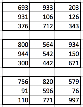
Figure 1: Three dimensional input hypermatrix example for algorithm 2

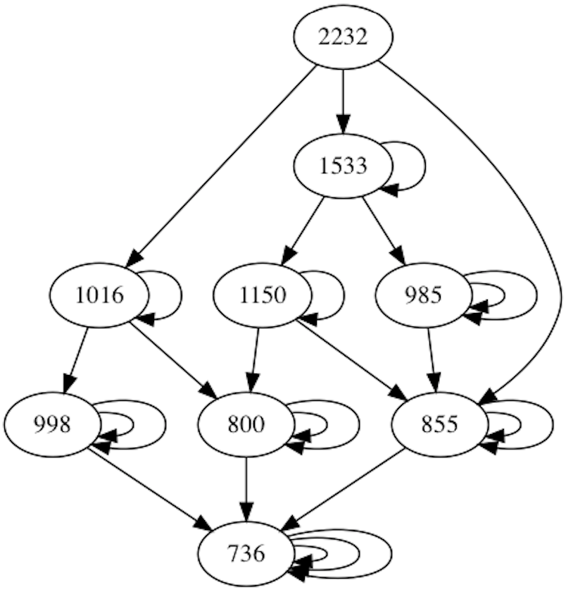
Figure 2: VLSN for matrix at figure 1. Starting solution is (693,542,997) = 2232; result is (203, 442, 91) = 736

Figure 2 shows example output graph generated by algorithm 2 with input matrix as in figure 1.

In Algorithm 2, the steepest descent through dimensions is described. Besides the steepest descent, the following variants of this search can be considered.

• Best improvement-based solution update (place a taboo on checking dimension $k^{\prime}$ in the next step).

• First improvement-based solution update (continue in new directions by increasing dimensions $k=k^{\prime}+1,\ldots$ or revisit previous directions by decreasing $k=k^{\prime}-1,\ldots$, placing a taboo on checking dimension $k^{\prime}$ in the next step).

• Random choice among improving solutions (with taboo on dimension $k^{\prime}$ in the next iteration).

4.3 Multi-start strategies for the VLSN search

The exploration stage of the VLSNS metaheuristic includes construction of another feasible solution from which the local search is to be restated. Multi-start strategy is a systematic way of constructing starting solutions. The original paper kammerdiner2017very that introduces the VLSNS metaheuristic describes two types of multi-start strategies, namely a random sampling strategy and a design based strategy. Using design based multi-start strategy in kammerdiner2017very , we propose a grid based strategy and compare the grid-based multi-start to random sampling multi-start. In particular, we modify the (random) design based restarts into the grid based restarts by using an identity permutation in place of a randomly generated permutation in the construction of starting solutions.

In combinatorics, a cyclic permutation is typically defined as a permutation which shifts all its elements $\{1,\ldots,N\}$ by a fixed offset, so that the elements moved off the end are inserted at the beginning of the permutation. In kammerdiner2017very , authors consider two types of cyclical permutations applied on a given permutation $\pi=(\pi(1),\ldots,\pi(N))$ of $N$-element set, namely

1. a $k$-push-up $\nu_{k}$:

   $$\nu_{k}(\pi(i))=\left\{\begin{array}[]{rl}\pi(i+k)&\textrm{for }i=1,\ldots,N-k,\\ \pi(i+k-N)&\textrm{for }i=N-k+1,\ldots,N.\end{array}\right.$$ (37)

2. a $k$-push-down $\delta_{k}$:

   $$\delta_{k}(\pi(i))=\left\{\begin{array}[]{rl}\pi(N+i-k)&\textrm{for }i=1,\ldots,k,\\ \pi(i-k)&\textrm{for }i=k+1,\ldots,N.\end{array}\right.$$ (40)

where $k$ is an integer $k=1,\ldots,N-1$.

Algorithm 3 Grid Multi-Start for Very Large-Scale Search

1:  Input $M$, $N$, and an initial permutation $\pi$ (e.g., $\pi=\iota=(1,2,\ldots,N)$)

2:  Initialize permutation subset to $\Pi_{0}\leftarrow\{\pi\}$

3:  for  position offset $k=1$ to $N-1$ do

4:     Construct $k$-push-up $\nu_{k}\leftarrow\nu_{k}(\pi)$

5:     Add $\nu_{k}$ to $\Pi_{0}$: $\Pi_{0}\leftarrow\Pi_{0}\cup\{\nu_{k}\}$

6:  end for

7:  Initialize multi-start (feasible) solutions set $\Sigma\leftarrow\varnothing$

8:  for number of starting solutions $\mu=1$ to $N^{M-1}$ do

9:     $S_{\mu}\leftarrow(\pi,\pi_{2},\ldots,\pi_{M})$, where $\pi_{j}\in\Pi_{0}$ for $j=2,\ldots,M$

10:     Add $S_{\mu}$ to $\Sigma$: $\Sigma\leftarrow\Sigma\cup\{S_{\mu}\}$

11:  end for

12:  Output a multi-start strategy $\Sigma=\{S_{1},\ldots,S_{\mu}\}$ with $\mu=N^{M-1}$

5 Complexity

The MAP is NP-hard (Karp, 1972). Next, we discuss an approach to evaluating the complexity of the VLSN search. In particular, we show that the search tree admits a partition of its nodes into the levels. These levels are ordered based on the MAP dimensions, which can be searched further. We use the partition of nodes into the levels in the search tree to define two related absorbing Markov chains. These two Markov chains allow us to obtain the upper bound on the expected number of moves through partition levels until reaching a local optimum.

To evaluate complexity of the VLSN search algorithm, observe that this algorithm works by successively searching through dimensions $1,2,\ldots,M$. Let $y$ and $y^{\prime}$ denote objective values of the current solution $S$ and the neighboring solution $S^{\prime}$. A starting solution or the current solution $S$ has some $I\leq M$ dimensions $m_{1},m_{2},\ldots,m_{I}$ that lead to improved objective value $y^{\prime}<y$. For the remaining $M-I\geq 0$ dimensions, there is no improvement as the neighborhood search returns $y^{\prime}=y$. Let us refer to the former $I$ dimensions as the improving dimensions of the current solution $S$, while the latter $M-I$ dimensions are called non-improving dimensions. The numbers of improving and non-improving dimensions $I,M-I\in\{0,1,\ldots,M\}$. This introduces a natural partition of the search tree of this algorithm into $M+1$ levels according to the specific number $I$ of improving dimensions that remain.

To illustrate this partition, consider, for example, a search tree in Fig. 2 for the MAP with $M=3,n=3$. The source node depicts a starting solution with objective value $2232$. The source node has an outdegree of three that corresponds to three improving dimensions, i.e., the source node belongs to the $I=3$ level. The intermediate nodes with objective values $1533,1150,1016$ have outdegree two each (not counting the self-loops) and belong to the $I=2$ level. Whereas the intermediate nodes with objective values $998,985,855,800$ have outdegree one each and belong to the $I=1$ level. The sink node with the (local and global) minimum objective value $736$ has a zero outdegree and belongs to the $I=0$ level in the search tree. Observe that the $I=2$ level’s node with value $1533$ leads to either another node (value $1150$) on the same $I=2$ level or the node (value $985$) on the lower level $I=1(=2-1)$. Interestingly, the source node (value $2232$) cannot stay on the same top level $I=3$ and instead leads to either the $I=2$ level nodes or the $I=1$ level node (value $855$). That is because an improving dimension that is used cannot be replaced with any other previously improved-on dimension.

As the algorithm progresses, the current solution moves from $S$ with $y$ and $I$ to its neighboring solution $S^{\prime}$ with $y^{\prime}<y$ and $I^{\prime}$. It is easy to see that for the VLSN search algorithm, we have:

1. if $I=M$ then $I^{\prime}\in\{I-1,I-2,\ldots,0\}$;

2. if $I=1,\ldots,M-1$ then $I^{\prime}\in\{I,I-1,\ldots,0\}$;

3. if $I=0$ then $I^{\prime}=\emptyset$.

In fact, $S$ and $S^{\prime}$ only differ in one dimension $k^{\ast}$, and by construction of the VLSN search no further improvements can be made through that dimension from $S^{\prime}$. If the current solution $S$ has $I=M$ then this solution is on the top level of the search tree. So, there are no dimensions that have been explored before such $S$. That means that its neighborhood solution $S^{\prime}$ cannot remain on the top level. Instead such $S^{\prime}$ must have $I^{\prime}<I$. On the other hand, if the current solution $S$ has $0<I<M$ then its neighborhood solution $S^{\prime}$ could have an improvement in some previously explored dimension $k_{1}$ (through which $S^{\prime}$ would have a neighbor $S_{1}$ with value $y_{1}$) as long as $y_{1}<y^{\prime}$. This means that for the levels $I=1,\ldots,M-1$, it is possible for $S^{\prime}$ to remain at the same level $I$ as $S$ after an objective-value improving move. Obviously, if the current solution $S$ has $I=0$ then no dimensions with improving moves remain, and so the current solution is a local (or global) optimum.

Next, we define two related Markov chains that allow us to evaluate the expected number of transitions through intermediate levels before reaching a minimum. The first Markov chain corresponds with the VLSN search through the levels, with the $I=0$ level as an absorbing state. The second Markov chain simplifies the evaluation of the first passage times in comparison with the first Markov chain.

For any $I_{0},I_{1}=0,1,\ldots,M$, let $p(I_{0},I_{1})=\Pr(I_{0}^{\prime}=I_{1})$ denote the probability of the number of improving dimensions changing from $I_{0}$ to $I_{1}$ when the VLSN search moves from $S_{0}$ and $S_{1}$. Now let us define a Markov chain $C$ with $M+1$ states corresponding to the levels of the search tree with a given number $I$ of the remaining improving dimensions. This Markov chain has an absorbing state at $I=0$, as the VLSN search algorithm stops when a local optimum is reached and no improving moves can be made. Consider the transition matrix $P=(P_{ij})_{i,j=0}^{M}$ of this Markov chain $C$.

$$P=\left(\begin{array}[]{cccccc}1&0&0&\ldots&0&0\\ p(1,0)&p(1,1)&0&\ldots&0&0\\ \vdots&\vdots&\vdots&\ddots&\vdots&\vdots\\ p(M-1,0)&p(M-1,1)&&\ldots&p(M-1,M-1)&0\\ p(M,0)&p(M,1)&p(M,2)&\ldots&p(M,M-1)&0\end{array}\right)$$ (41)

To get an upper bounds for the expected number of transitions before reaching the absorbing state for Markov chain $C$, consider a related Markov chain $C_{1}$ whose transition matrix $P_{1}$ is based on the transition probabilities.

$$P_{1}=\left(\begin{array}[]{ccccccc}1&0&0&\ldots&0&0&0\\ 1-p(1,1)&p(1,1)&0&\ldots&0&0&0\\ \vdots&\vdots&\vdots&\ddots&\vdots&\vdots&\vdots\\ 0&0&0&\ldots&1-p(M-1,M-1)&p(M-1,M-1)&0\\ 0&0&0&\ldots&0&1&0\end{array}\right)$$ (42)

Let $\nu_{I}$, $I=0,1,\ldots,M$ denote the expected number of transitions in this Markov chain $C_{1}$ starting in state $I$ before reaching the absorbing state $I=0$, i.e. local minimum. Note that $\nu_{0}=0$ and for any $0<I<M$, $\nu_{I}=1+p_{I,I}\nu_{I}+(1-p_{I,I})\nu_{I-1}$ or $\nu_{I}=\nu_{I-1}+\frac{1}{1-p_{I,I}}$. Hence, $\nu_{I}=\sum_{i=1}^{I}\frac{1}{1-p_{i,i}}$ for $I=1,2,\ldots,M-1$. Also, $\nu_{M}=1+\nu_{M-1}=1+\sum_{i=1}^{M-1}\frac{1}{1-p_{i,i}}$.

The Hungarian algorithm for solving the LAP in each dimension has complexity of order $n^{3}$. Whereas the complexity of extracting the matrix of cost coefficients for the LAP (i.e., getting the projection $C(k,S)$ of multidimensional cost array $C$) has order $n^{2}$. The expected number of times the VLSN search repeatedly solves the Hungarian algorithm does not exceed $\mu M\nu_{M}=\mu M\left(1+\sum_{i=1}^{M-1}\frac{1}{1-p_{i,i}}\right)$. Hence, the VLSN search has the worst-case complexity of $n^{3}\mu M\nu_{M}$.

6 Numerical experiments

The main goal of our numerical studies is to document and compare the performance of two recent heuristics developed for general MAPs of large size. Additionally, we want to understand the extent to which different exploration or multi-start strategies can influence the solutions returned by the VLSN search algorithm. This is particularly important because kammerdiner2017very proposed two distinct multi-start strategies but have not studied or compared them numerically.

Specifically, we have implemented two algorithms described above, and performed experiments, aimed at answering the following questions:

1. Does the VLSN search result in better MAP solutions than those produced by Greedy algorithm?

2. Does a multi-start VLSN search strategy improve the found solution when compared to a single-start?

3. Does the use of greedy algorithm’s solution as the starting solution for the VLSN search improve the found solution when compared to the VLSN search started at a randomly constructed feasible solution?

4. How does the grid compare to the random start?

The algorithms were implemented in C++; the code was executed in sequential manner using 40 core Intel(R) Xeon(R) CPU E5-2640 v4 @ 2.40GHz processor with 256 GB RAM. Optimal solutions were obtained using Gurobi 9.0 solver on the same computer, using 20 threads. In Gurobi, we have set timelimit 10 minutes for each of the problems. While running VLSN we have set limit on number of explored nodes for instances with M = 3 and N = 50 (250000 nodes), and N = 100 (400000 nodes), and with M = 4, N = 20 (1600000 nodes), and N = 30 (2700000 nodes).

We have implemented two versions of genetic algorithm, inspired by a random-key generic algorithm as described in 10.1007/s10898-013-0105-7 . As MAP is a constrained discrete optimization problem, we had to develop an encoding and decoding scheme that would satisfy problem constraints after the crossover operations. We have represented a chromosome as a matrix $M_{cd}$ where number of rows $c$ equals to problem cardinality, and number of columns $d$ to dimensionality of considered MAP. Then, each row of the matrix would represent coordinates of the cell of the MAP hypermatrix. Each column $i\in(1,...d)$ of $M_{cd}$ represents a permutation of elements $(1,...,c)$. MAP objective function value would then be equal to the sum of values corresponding to all cells in $M_{cd}$. Crossover operation producing one chromosome from two was implemented as a random combination of columns of two matrices $M^{1}_{cd}$ and $M^{2}_{cd}$. Each evolution step was taking $p\%$ of the best (“elitist”) solutions, performing crossover resulting in $r\%$ of new chromosomes, merging the results with $q<p$% top solutions and generating remaining population randomly. We have implemented two versions of genetic algorithm: GA1 had $p$ set to 60%, $q$ to 20%, and $r$ to 60%, and GA2 had $p$ set to 40% (thus, only “elite” 20% and remaining 20% were involved in the crossover). GA1 had 2000 evolution steps, GA2 had 5000 steps.

We have generated random hypermatrices of different dimensions $M$ and cardinalities $N$, and solved the MAP for these synthetic matrices. Matrix elements contain uniformly distributed random numbers in the range from 0 to 1. Results of the experiment are shown in Tables  LABEL:exp-3AP and LABEL:exp-4AP. These tables show pairwise comparisons of several versions of the VLSN search with greedy algorithms, genetic algorithms, and all-purpose solver Gurobi 9. These include the VLSN search with a single starting solution (denoted by VLSN1), the VLSN search with multiple starts (denoted by VLSNMS), a greedy algorithm (denoted by Greedy), the VLSN search which uses deterministic grid-based strategy to construct starting feasible solutions (denoted by Grid-VLSN), and a hybridization of the VLSN search with greedy algorithm, where the VLSN search uses the solution found by greedy procedure as a starting solution. For each of these algorithms, we record the (best or smallest local optimal) values $y_{\textrm{alg}}^{i}$ of the solutions found by the algorithm for a given problem instance $i\in\{1,\ldots,I\}$and compare these values using statistical approaches.

We present and discuss the results of statistical comparison of VLSN and non-VLSN algorithms in Section 6.1. As the size $N^{M}$ of hypermatrix of cost coefficients grows exponentially with the dimensionality $M$, we limit our numerical experiments to the MAP instances with $M=3,4$. For the 3-AP, we consider instances with cardinality $N=3,10,20,30,40,50,100$. While for the 4-AP, we consider $N=3,10,20,30$. Although the MAP instances with $N=3$ are trivial having the input size of 27 or 81 cost coefficients, the larger cardinality $N$ values in our experiments produce hypermatrices with 1,000,000 and 810,000 coefficients and instances with $100!^{2}$ and $30!^{3}$ feasible solutions for this generally NP-hard problem.

Furthermore, we illustrate the application of our MAP-based approach to solving multipartite entity resolution problem from computer science in Section 6.2. We show that VLSN-based approaches such as Greedy-VLSN can perform well when matching data from three datasets or sources with various degree of dissimilarity in the records contained in different sources (i.e., datasets).

6.1 Statistical comparison of the solution quality for the VLSN search and alternative algorithms

We compare the quality of solutions found by various versions of the VLSN search and alternative algorithms, including metaheuristics, Greedy heuristic, and a standard solver such as Gurobi. In particular, the comparisons are performed on sets of randomly generated problem instances for given cardinality ($n$) and dimensionality ($M$) parameters of the MAP. To perform proper statistical comparisons among the algorithms, we fix the MAP parameters $n,M$ and choose pairs $(A_{1},A_{2})$ of algorithms to compare so that Algorithm 1, $A_{1}$, is a version of the VLSN search (e.g., a grid multi-start VLSN search, or a hybrid VLSN search with a start at Greedy solution), and Algorithm 2, $A_{2}$ is an alternative, non-VLSN algorithm (e.g., a Genetic algorithm GA, a Greedy algorithm, Gurobi, etc.).

Let $y_{1},y_{2}$ (and $T_{1},T_{2}$) denote the objective values (and the number of solutions explored) that are found by algorithms $A_{1},A_{2}$. Recall that $A_{1}$ always stands for some VLSN algorithm while $A_{2}$ is non-VLSN, and consider a difference $y_{1}-y_{2}$ between their returned objective values (alternatively, $T_{1}-T_{2}$ is a difference in the number of searched solutions between $A_{1}$ and $A_{2}$). This difference $y_{1}-y_{2}$ is positive, when the quality of solution found by the VLSN search is better than its alternative’s $A_{2}$. For some of $I=100$ randomly generated problem instances, the $y_{1}-y_{2}$ differences are randomly distributed. Recall that the objective values $y_{1},y_{2}$ are sums of randomly generated cost coefficients. So, by the law of large numbers, for large cardinality $n$, the difference $y_{1}-y_{2}$ is approximately normally distributed as a difference of approximately normal $y_{i},i=1,2$.

To statistically compare the solution qualities, we construct a confidence interval for $y_{1}-y_{2}$, where the observed differences are taken between $y_{1}=y_{1}(i)$ and $y_{2}=y_{2}(i)$ when $A_{1},A_{2}$ are ran on the same problem instance $\mathrm{MAP}_{i}(n,M)$ where $n,M$ are the cardinality and the dimensionality, and $i=1,2,\ldots,I$. To construct the confidence intervals, find the sample mean

$$\color[rgb]{1,0,0}A_{1,2}=\widehat{y_{2}-y_{1}}=\frac{1}{I}\sum_{i=1}^{I}\left(y_{2}(i)-y_{1}(i)\right),$$

and the sample standard deviation $\color[rgb]{1,0,0}D_{1,2}=\sqrt{\frac{1}{I-1}\sum_{i=1}^{I}\left(y_{2}(i)-y_{1}(i)-A_{1,2}\right)^{2}}.$ Given a p-value of $0.05$, the 95%-confidence interval for the difference $y_{2}-y_{1}$ is

$$\color[rgb]{1,0,0}\left(A_{1,2}-t_{1-\alpha/2,I-1}\cdot\frac{D_{1,2}}{\sqrt{I-1}},\quad A_{1,2}+t_{1-\alpha/2,I-1}\cdot\frac{D_{1,2}}{\sqrt{I-1}}\right),$$

where $t_{\alpha}$ is the $\alpha$-th percentile of the t-distribution. Here, we use $\alpha=0.05$, $I-1=99$, and $t_{1-\alpha/2,I-1}=t_{0.975,99}=1.984$.

We compute $A_{1,2}$, $D_{1,2}$, and the confidence intervals for all possible combinations of the VLSN search variants $A_{1}$ and the alternative, non-VLSN solution algorithms $A_{2}$. Using the confidence intervals, we interpret the results of comparison as follows. If zero does not belong to the confidence interval, then the difference in performance (i.e., solution quality) between $A_{1}$ and $A_{2}$ is statistically significant. Moreover, the VLSN search outperforms if $\color[rgb]{1,0,0}0<A_{1,2}-t_{1-\alpha/2,I-1}\cdot\frac{D_{1,2}}{\sqrt{I-1}}$, or equivalently $\color[rgb]{1,0,0}A_{1,2}>t_{1-\alpha/2,I-1}\cdot\frac{D_{1,2}}{\sqrt{I-1}}$. Otherwise the non-VLSN algorithm outperforms if $\color[rgb]{1,0,0}A_{1,2}+t_{1-\alpha/2,I-1}\cdot\frac{D_{1,2}}{\sqrt{I-1}}<0$, or $\color[rgb]{1,0,0}A_{1,2}<-t_{1-\alpha/2,I-1}\cdot\frac{D_{1,2}}{\sqrt{I-1}}$.

Observe that most pairs of VLSN and non-VLSN algorithms $A_{1},A_{2}$ are not based on each other. The only exception from this rule is comparison between Greedy-VLSN (a hybridized VLSN with Greedy solutions as its starts) and Greedy (non-VLSN). By construction, Greedy-VLSN is guaranteed to always do at least as good as Greedy on the same problem instance. So, the differences of these two will follow a log-normal distribution rather than be approximately normally distributed, since there is a dependence. Hence, we modify the construction of the confidence intervals for these two algorithms.

First, for the Greedy-VLSN and Greedy algorithms $A_{1},A_{2}$, we calculate the sample means and standard deviations for the logged differences:

$$\color[rgb]{1,0,0}A_{1,2}=\widehat{\log(y_{2}-y_{1})}=\frac{1}{I}\sum_{i=1}^{I}\log\left(y_{2}(i)-y_{1}(i)\right),$$

and

$$\color[rgb]{1,0,0}D_{1,2}=\sqrt{\frac{1}{I-1}\sum_{i=1}^{I}\left(\log\left(y_{2}(i)-y_{1}(i)\right)-A_{1,2}\right)^{2}},$$

where $\log(\cdot)$ represents a natural logarithm.

Using a modified Cox method zhou1997confidence suggested for moderate sample sizes $I=100\geq 50$, a 95% confidence interval for the log-difference $\log(y_{2}-y_{1})$ between Greedy-VLSN $A_{1}$ and Greedy $A_{2}$ is

$$\color[rgb]{1,0,0}(\log L,\log U)=\left(A_{1,2}+\frac{D_{1,2}^{2}}{2}\pm t_{1-\alpha/2}\sqrt{\frac{D_{1,2}^{2}}{2}+\frac{D_{1,2}^{4}}{2(I-1)}}\right),$$

where $t_{\alpha}$ is the $\alpha$-th percentile of the t-distribution. Here again, we use $\alpha=0.05$, $I-1=99$, and $t_{1-\alpha/2,I-1}=t_{0.975,99}=1.984$. Then a 95% confidence interval for the difference $(y_{2}-y_{1})$ between Greedy-VLSN $A_{1}$ and Greedy $A_{2}$ is

$$\color[rgb]{1,0,0}(L,U)=\left(\exp\left\{A_{1,2}+\frac{D_{1,2}^{2}}{2}\pm t_{1-\alpha/2}\sqrt{\frac{D_{1,2}^{2}}{2}+\frac{D_{1,2}^{4}}{2(I-1)}}\right\}\right),$$

The results of the comparison for the MAP with $M=3$ and $M=4$ are summarized in Tables LABEL:exp-3AP and LABEL:exp-4AP, respectively. With exception of the small-size MAP with $M=3,n=3$ or $M=4,n=4$, VLSN algorithms outperforms Greedy and both genetic algorithms. As the cardinality and the size of instances grow, the random multi-start search (VLSNMS) seems to perform the best among the tested heuristics, as evident from the comparison with Gurobi. However, the deterministic grid-based multi-start (Grid-VLSN) begin to outperform the random multi-start search as the cardinality becomes sufficiently high (e.g., the 3-APs with $n=100$ and the 4-APs with $n=20,30$. This suggests that due to the space-filling property of this design-based multi-start kammerdiner2017very , the grid-based multi-start strategy tends to result in exploration of more diverse or expansive set of solutions. On the other hand, the use of Greedy solution as a start in the VLSN search may improve the performance. In fact, for the 3-APs with $N=50$ and $N=100$, hybrid Greedy-VLSN search significantly outperforms other tested heuristics.

Table 2: Statistical Comparison of Experiments for $M=3$

$A_{1}$:	$A_{2}$:	M	n	Mean	Std. $D_{1,2}$	95% C.I.	Winner
VLSN	Non-VLSN			$A_{1,2}$
VLSN1	Greedy	3	3	214342.030	229466.388	(168586.546, 260097.514)	VLSN
	GA1	3	3	-7695.080	45128.527	(-16693.686, 1303.526)	None
	GA2	3	3	-7695.080	45128.527	(-16693.686, 1303.526)	None
	Gurobi	3	3	-7695.080	45128.527	(-16693.686, 1303.526)	None
VLSNMS	Greedy	3	3	223494.530	223403.268	(178948.029, 268041.031)	VLSN
	GA1	3	3	1457.420	12369.498	(-1009.052, 3923.892)	None
	GA2	3	3	1457.420	12369.498	(-1009.052, 3923.892)	None
	Gurobi	3	3	1457.420	12369.498	(-1009.052, 3923.892)	None
Grid-VLSN	Greedy	3	3	223494.530	223403.268	(178948.029, 268041.031)	VLSN
	GA1	3	3	1457.420	12369.498	(-1009.052, 3923.892)	None
	GA2	3	3	1457.420	12369.498	(-1009.052, 3923.892)	None
	Gurobi	3	3	1457.420	12369.498	(-1009.052, 3923.892)	None
Greedy-VLSN	Greedy	3	3	209645.460	230090.725	(3225943.686, 810173971774378.625)	VLSN
	GA1	3	3	-12391.650	41144.578	(-20595.858, -4187.442)	Non-VLSN
	GA2	3	3	-12391.650	41144.578	(-20595.858, -4187.442)	Non-VLSN
	Gurobi	3	3	-12391.650	41144.578	(-20595.858, -4187.442)	Non-VLSN
VLSN1	Greedy	3	10	542017.770	315482.629	(479110.691, 604924.849)	VLSN
	GA1	3	10	760288.510	175283.909	(725336.986, 795240.034)	VLSN
	GA2	3	10	769004.430	181455.812	(732822.231, 805186.629)	VLSN
	Gurobi	3	10	-128186.000	70074.942	(-142158.909, -114213.091)	Non-VLSN
VLSNMS	Greedy	3	10	665923.850	313330.992	(603445.806, 728401.894)	VLSN
	GA1	3	10	884194.590	154886.611	(853310.277, 915078.903)	VLSN
	GA2	3	10	892910.510	167886.376	(859434.050, 926386.970)	VLSN
	Gurobi	3	10	-4279.920	12186.237	(-6709.850, -1849.990)	Non-VLSN
Grid-VLSN	Greedy	3	10	629492.110	318919.295	(565899.761, 693084.459)	VLSN
	GA1	3	10	847762.850	156755.347	(816505.912, 879019.788)	VLSN
	GA2	3	10	856478.770	169972.853	(822586.268, 890371.272)	VLSN
	Gurobi	3	10	-40711.660	32373.959	(-47167.011, -34256.309)	Non-VLSN
Greedy-VLSN	Greedy	3	10	542307.910	320121.278	(156061.777, 4065828346.104)	VLSN
	GA1	3	10	760578.650	165832.273	(727511.777, 793645.523)	VLSN
	GA2	3	10	769294.570	196599.749	(730092.678, 808496.462)	VLSN
	Gurobi	3	10	-127895.860	87987.696	(-145440.563, -110351.157)	Non-VLSN
VLSN1	Greedy	3	20	585363.040	307288.252	(524089.915, 646636.165)	VLSN
	GA1	3	20	3823013.580	300278.765	(3763138.144, 3882889.016)	VLSN
	GA2	3	20	3835849.410	295563.710	(3776914.153, 3894784.667)	VLSN
	Gurobi	3	20	-236083.590	52816.299	(-246615.134, -225552.046)	Non-VLSN
VLSNMS	Greedy	3	20	722671.110	303454.217	(662162.490, 783179.730)	VLSN
	GA1	3	20	3960321.650	298155.840	(3900869.524, 4019773.776)	VLSN
	GA2	3	20	3973157.480	301518.528	(3913034.836, 4033280.124)	VLSN
	Gurobi	3	20	-98775.520	20701.131	(-102903.315, -94647.725)	Non-VLSN
Grid-VLSN	Greedy	3	20	672606.190	304057.858	(611977.204, 733235.176)	VLSN
	GA1	3	20	3910256.730	293280.628	(3851776.719, 3968736.741)	VLSN
	GA2	3	20	3923092.560	306168.609	(3862042.692, 3984142.428)	VLSN
	Gurobi	3	20	-148840.440	26144.873	(-154053.715, -143627.165)	Non-VLSN
Greedy-VLSN	Greedy	3	20	640749.880	309907.226	(65603.813, 18985277.328)	VLSN
	GA1	3	20	3878400.420	299689.695	(3818642.444, 3938158.396)	VLSN
	GA2	3	20	3891236.250	310487.262	(3829325.244, 3953147.256)	VLSN
	Gurobi	3	20	-180696.750	56969.899	(-192056.520, -169336.980)	Non-VLSN
VLSN1	Greedy	3	30	547523.710	287548.220	(490186.738, 604860.682)	VLSN
	GA1	3	30	7434182.070	426287.497	(7349180.555, 7519183.585)	VLSN
	GA2	3	30	7499214.450	292365.595	(7440916.896, 7557512.004)	VLSN
	Gurobi	3	30	-272285.320	32905.022	(-278846.565, -265724.075)	Non-VLSN
VLSNMS	Greedy	3	30	659756.550	291005.873	(601730.124, 717782.976)	VLSN
	GA1	3	30	7546414.910	428167.560	(7461038.512, 7631791.308)	VLSN
	GA2	3	30	7611447.290	290447.548	(7553532.193, 7669362.387)	VLSN
	Gurobi	3	30	-160052.480	15141.474	(-163071.682, -157033.278)	Non-VLSN
Grid-VLSN	Greedy	3	30	619527.740	291727.276	(561357.466, 677698.014)	VLSN
	GA1	3	30	7506186.100	432202.493	(7420005.138, 7592367.062)	VLSN
	GA2	3	30	7571218.480	287537.072	(7513883.731, 7628553.229)	VLSN
	Gurobi	3	30	-200281.290	21595.991	(-204587.520, -195975.060)	Non-VLSN
Greedy-VLSN	Greedy	3	30	623372.170	282526.737	(104743.167, 536568.429)	VLSN
	GA1	3	30	7510030.530	430923.987	(7424104.501, 7595956.559)	VLSN
	GA2	3	30	7575062.910	283967.037	(7518440.024, 7631685.796)	VLSN
	Gurobi	3	30	-196436.860	45216.148	(-205452.937, -187420.783)	Non-VLSN
VLSN1	Greedy	3	40	632734.380	310776.474	(570765.706, 694703.054)	VLSN
	GA1	3	40	11370163.470	450560.750	(11280321.881, 11460005.059)	VLSN
	GA2	3	40	11159395.770	412442.699	(11077154.901, 11241636.639)	VLSN
	Gurobi	3	40	-301675.170	33257.627	(-308306.724, -295043.616)	Non-VLSN
VLSNMS	Greedy	3	40	741892.330	308895.953	(680298.631, 803486.029)	VLSN
	GA1	3	40	11479321.420	445664.135	(11390456.213, 11568186.627)	VLSN
	GA2	3	40	11268553.720	410541.045	(11186692.040, 11350415.400)	VLSN
	Gurobi	3	40	-192517.220	13239.799	(-195157.229, -189877.211)	Non-VLSN
Grid-VLSN	Greedy	3	40	702126.210	310744.835	(640163.844, 764088.576)	VLSN
	GA1	3	40	11439555.300	446812.411	(11350461.127, 11528649.473)	VLSN
	GA2	3	40	11228787.600	412326.091	(11146569.983, 11311005.217)	VLSN
	Gurobi	3	40	-232283.340	19798.391	(-236231.129, -228335.551)	Non-VLSN
Greedy-VLSN	Greedy	3	40	738094.340	302753.314	(79306.429, 4576228.208)	VLSN
	GA1	3	40	11475523.430	450631.897	(11385667.654, 11565379.206)	VLSN
	GA2	3	40	11264755.730	411792.814	(11182644.448, 11346867.012)	VLSN
	Gurobi	3	40	-196315.210	42157.588	(-204721.412, -187909.008)	Non-VLSN
VLSN1	Greedy	3	50	532389.470	305910.186	(471391.131, 593387.809)	VLSN
	GA1	3	50	15283969.450	570429.146	(15170226.162, 15397712.738)	VLSN
	GA2	3	50	15099111.000	503005.517	(14998811.950, 15199410.050)	VLSN
	Gurobi	3	50	-378638.790	39552.538	(-386525.546, -370752.034)	Non-VLSN
VLSNMS	Greedy	3	50	663933.540	303157.072	(603484.171, 724382.909)	VLSN
	GA1	3	50	15415513.520	568004.680	(15302253.669, 15528773.371)	VLSN
	GA2	3	50	15230655.070	504040.517	(15130149.642, 15331160.498)	VLSN
	Gurobi	3	50	-247094.720	13459.298	(-249778.497, -244410.943)	Non-VLSN
Grid-VLSN	Greedy	3	50	656987.910	307018.338	(595768.606, 718207.214)	VLSN
	GA1	3	50	15408567.890	568944.808	(15295120.578, 15522015.202)	VLSN
	GA2	3	50	15223709.440	503299.612	(15123351.748, 15324067.132)	VLSN
	Gurobi	3	50	-254040.350	14541.767	(-256939.971, -251140.729)	Non-VLSN
Greedy-VLSN	Greedy	3	50	717863.920	302082.191	(132413.175, 547247.574)	VLSN
	GA1	3	50	15469443.900	569746.864	(15355836.659, 15583051.141)	VLSN
	GA2	3	50	15284585.450	505483.372	(15183792.317, 15385378.583)	VLSN
	Gurobi	3	50	-193164.340	32610.082	(-199666.774, -186661.906)	Non-VLSN
VLSN1	Greedy	3	100	432980.030	308760.169	(371413.406, 494546.654)	VLSN
	GA1	3	100	36266744.820	641765.795	(36138777.040, 36394712.600)	VLSN
	GA2	3	100	35997235.880	725050.818	(35852661.107, 36141810.653)	VLSN
	Gurobi	3	100	-446354.930	37218.735	(-453776.327, -438933.533)	Non-VLSN
VLSNMS	Greedy	3	100	572240.510	312392.330	(509949.635, 634531.385)	VLSN
	GA1	3	100	36406005.300	638373.264	(36278713.989, 36533296.611)	VLSN
	GA2	3	100	36136496.360	728320.389	(35991269.637, 36281723.083)	VLSN
	Gurobi	3	100	-307094.450	10890.716	(-309266.053, -304922.847)	Non-VLSN
Grid-VLSN	Greedy	3	100	594828.740	312548.849	(532506.655, 657150.825)	VLSN
	GA1	3	100	36428593.530	638288.430	(36301319.135, 36555867.925)	VLSN
	GA2	3	100	36159084.590	727803.960	(36013960.843, 36304208.337)	VLSN
	Gurobi	3	100	-284506.220	10877.640	(-286675.216, -282337.224)	Non-VLSN
Greedy-VLSN	Greedy	3	100	726941.570	309360.760	(134148.649, 551656.943)	VLSN
	GA1	3	100	36560706.360	634202.488	(36434246.699, 36687166.021)	VLSN
	GA2	3	100	36291197.420	726377.431	(36146358.122, 36436036.718)	VLSN
	Gurobi	3	100	-152393.390	24995.680	(-157377.516, -147409.264)	Non-VLSN

Table 3: Statistical Comparison of Experiments for $M=4$

$A_{1}$:	$A_{2}$:	M	n	Mean	Std. $D_{1,2}$	95% C.I.	Winner
VLSN	Non-VLSN			$A_{1,2}$
VLSN1	Greedy	4	4	420708.680	291983.871	(362487.241, 478930.119)	VLSN
	GA1	4	4	-33290.710	64040.578	(-46060.369, -20521.051)	Non-VLSN
	GA2	4	4	-33290.710	64040.578	(-46060.369, -20521.051)	Non-VLSN
	Gurobi	4	4	-33290.720	64040.574	(-46060.379, -20521.061)	Non-VLSN
VLSNMS	Greedy	4	4	453999.390	273321.510	(399499.217, 508499.563)	VLSN
	GA1	4	4	0.000	0.000	(0.000, 0.000)	Tie
	GA2	4	4	0.000	0.000	(0.000, 0.000)	Tie
	Gurobi	4	4	-0.010	0.100	(-0.030, 0.010)	None
Grid-VLSN	Greedy	4	4	453999.390	273321.510	(399499.217, 508499.563)	VLSN
	GA1	4	4	0.000	0.000	(0.000, 0.000)	Tie
	GA2	4	4	0.000	0.000	(0.000, 0.000)	Tie
	Gurobi	4	4	-0.010	0.100	(-0.030, 0.010)	None
Greedy-VLSN	Greedy	4	4	342323.700	286661.924	(6464833.248, 884074728781398.875)	VLSN
	GA1	4	4	-111675.690	118453.291	(-135295.217, -88056.163)	Non-VLSN
	GA2	4	4	-111675.690	118453.291	(-135295.217, -88056.163)	Non-VLSN
	Gurobi	4	4	-111675.700	118453.283	(-135295.226, -88056.174)	Non-VLSN
VLSN1	Greedy	4	10	457756.410	303442.832	(397250.060, 518262.760)	VLSN
	GA1	4	10	849064.340	157667.201	(817625.579, 880503.101)	VLSN
	GA2	4	10	944836.200	122696.744	(920370.530, 969301.870)	VLSN
	Gurobi	4	10	-168329.980	35154.080	(-175339.686, -161320.274)	Non-VLSN
VLSNMS	Greedy	4	10	580535.270	296673.117	(521378.798, 639691.742)	VLSN
	GA1	4	10	971843.200	145473.373	(942835.882, 1000850.518)	VLSN
	GA2	4	10	1067615.060	119273.555	(1043831.972, 1091398.148)	VLSN
	Gurobi	4	10	-45551.120	14835.867	(-48509.385, -42592.855)	Non-VLSN
Grid-VLSN	Greedy	4	10	567159.630	297875.243	(507763.455, 626555.805)	VLSN
	GA1	4	10	958467.560	144629.304	(929628.549, 987306.571)	VLSN
	GA2	4	10	1054239.420	120087.033	(1030294.125, 1078184.715)	VLSN
	Gurobi	4	10	-58926.760	15813.094	(-62079.883, -55773.637)	Non-VLSN
Greedy-VLSN	Greedy	4	10	471827.540	302512.696	(287030.494, 48785145828.742)	VLSN
	GA1	4	10	863135.470	154370.048	(832354.159, 893916.781)	VLSN
	GA2	4	10	958907.330	136883.720	(931612.784, 986201.876)	VLSN
	Gurobi	4	10	-154258.850	64071.598	(-167034.695, -141483.005)	Non-VLSN
VLSN1	Greedy	4	20	342618.340	295625.389	(283670.785, 401565.895)	VLSN
	GA1	4	20	3931114.510	337716.280	(3863774.052, 3998454.968)	VLSN
	GA2	4	20	3954816.290	282396.423	(3898506.584, 4011125.996)	VLSN
	Gurobi	4	20	-269337.000	32469.602	(-275811.423, -262862.577)	Non-VLSN
VLSNMS	Greedy	4	20	481352.330	295531.385	(422423.519, 540281.141)	VLSN
	GA1	4	20	4069848.500	333945.221	(4003259.989, 4136437.011)	VLSN
	GA2	4	20	4093550.280	282354.181	(4037248.997, 4149851.563)	VLSN
	Gurobi	4	20	-130603.010	10977.705	(-132791.959, -128414.061)	Non-VLSN
Grid-VLSN	Greedy	4	20	483696.310	294034.410	(425065.995, 542326.625)	VLSN
	GA1	4	20	4072192.480	333364.431	(4005719.778, 4138665.182)	VLSN
	GA2	4	20	4095894.260	282618.431	(4039540.285, 4152248.235)	VLSN
	Gurobi	4	20	-128259.030	10061.525	(-130265.293, -126252.767)	Non-VLSN
Greedy-VLSN	Greedy	4	20	468652.290	291875.195	(76908.751, 479624503.370)	VLSN
	GA1	4	20	4057148.460	333773.486	(3990594.193, 4123702.727)	VLSN
	GA2	4	20	4080850.240	286310.078	(4023760.153, 4137940.327)	VLSN
	Gurobi	4	20	-143303.050	43853.404	(-152047.397, -134558.703)	Non-VLSN
VLSN1	Greedy	4	30	301879.240	299150.600	(242228.759, 361529.721)	VLSN
	GA1	4	30	7477163.470	324465.621	(7412465.187, 7541861.753)	VLSN
	GA2	4	30	7437036.990	369574.419	(7363344.035, 7510729.945)	VLSN
	Gurobi	4	30	-325354.810	37874.047	(-332906.876, -317802.744)	Non-VLSN
VLSNMS	Greedy	4	30	457678.140	293766.388	(399101.268, 516255.012)	VLSN
	GA1	4	30	7632962.370	322434.530	(7568669.085, 7697255.655)	VLSN
	GA2	4	30	7592835.890	365974.022	(7519860.852, 7665810.928)	VLSN
	Gurobi	4	30	-169555.910	10206.322	(-171591.046, -167520.774)	Non-VLSN
Grid-VLSN	Greedy	4	30	465655.330	295055.791	(406821.352, 524489.308)	VLSN
	GA1	4	30	7640939.560	323539.582	(7576425.928, 7705453.192)	VLSN
	GA2	4	30	7600813.080	364738.028	(7528084.499, 7673541.661)	VLSN
	Gurobi	4	30	-161578.720	10410.772	(-163654.623, -159502.817)	Non-VLSN
Greedy-VLSN	Greedy	4	30	503226.990	291500.030	(85368.942, 509448384.965)	VLSN
	GA1	4	30	7678511.220	324933.084	(7613719.725, 7743302.715)	VLSN
	GA2	4	30	7638384.740	364695.841	(7565664.571, 7711104.909)	VLSN
	Gurobi	4	30	-124007.060	35641.249	(-131113.907, -116900.213)	Non-VLSN

Column $A_{1}$: VLSN contains a name of VLSN version. Column $A_{2}$: Non-VLSN lists a name of non-VLSN algorithm that is compared with the VLSN search in the same row. Columns $A_{1,2}$, $D_{1,2}$, and 95% C.I. display the sample mean, the sample standard deviation, and the 95% confidence interval for $y_{1}-y_{2}$.

6.2 Illustration of application to multipartite entity resolution problem

Current experiment presents illustration of application of proposed algorithms to multipartite entity resolution problem. Experiment settings and results are displayed in table 5. We have collected list of 2610 highly cited researcher names from (http://www.webometrics.info/en/node/58) and selected subset of size N of their names. Next, we created three identical datasets $D_{1}$, $D_{2}$, and $D_{3}$. Column e denotes error: probability under which random letter of any item in $D_{1}$ or $D_{2}$ would be changed to random letter. Part of distorted dataset is shown in table 4. We have generated input matrix as per formulation 3, using trigram similarity as similarity function, and performed greedy search as in algorithm 1, and then improved it using VLSN with greedy start (alg. 2). Algorithms return solutions as set of 3-tuples $((d_{1}^{1},d_{2}^{1},d_{3}^{1}),...,(d_{1}^{N},d_{2}^{N},d_{3}^{N}))$, meaning that $d_{1}^{1}$, $d_{2}^{1}$, and $d_{3}^{1}$ denote the same entity. We define 3-tuple as correctly matched, if all its elements correspond to the record for the same entity, otherwise the 3-tuple is matched incorrectly. We define recall of the algorithm as the ratio of correctly matched 3-tuples to the total number of 3-tuples. Columns R(G) and R(V_G) denote recall for greedy and for VLSN-greedy algorithms respectively. Column $|V|$ denotes number of nodes in the resulting graph. Results of this experiment show that recall for VLSN search improves over greedy search.

Table 4: part of source data for e = 40

$D_{1}$	$D_{2}$	$D_{3}$
Sigmund Freud	Sigmund Freud	SigmundxFreuv
Graham Colditz	srShamNConditz	GrahaGOColditu
Ronald C Kessler	RLnald C KmsslXr	pocalt C KEssler
JoAnn E Manson	hoAnn AhYansan	JoAnniE Manson
Shizuo Akira	ShMzuI Tkila	zhizuoyAkCra

Table 5: Results of application of MAP to multipartite entity resolution problem

#	N	e	G	V_G	$|V|$	R(G)	R(V_G)
1	10	0	10	10	1	1.0	1.0
2	10	50	6	10	4	0.6	1.0
3	20	20	20	20	1	1.0	1.0
4	20	30	17	20	2	0.85	1.0
5	40	20	40	40	1	1.0	1.0
6	20	50	16	20	4	0.8	1.0
7	50	10	50	50	1	1.0	1.0
8	10	20	10	10	1	1.0	1.0
9	20	10	20	20	1	1.0	1.0
10	20	40	20	20	1	1.0	1.0
11	10	40	6	8	4	0.6	0.8
12	20	0	20	20	1	1.0	1.0
13	10	30	8	10	2	0.8	1.0
14	10	10	10	10	1	1.0	1.0
15	40	10	40	40	1	1.0	1.0
16	50	20	48	48	2	0.96	0.96
17	40	30	31	38	4	0.775	0.95
18	40	40	30	37	7	0.75	0.925
19	100	10	100	100	1	1.0	1.0
20	50	30	36	50	5	0.72	1.0
21	100	20	96	98	2	0.96	0.98
22	50	40	38	46	13	0.76	0.92
23	40	50	22	26	25	0.55	0.65
24	50	50	20	28	13	0.4	0.56
25	100	30	72	96	13	0.72	0.96
26	300	10	289	300	4	0.96	1.0
27	100	40	54	71	35	0.54	0.71
28	100	50	31	47	83	0.31	0.47
29	300	20	269	300	9	0.89	1.0
30	300	30	207	276	20	0.69	0.92
31	300	40	131	201	82	0.43	0.67

7 Conclusions and further research

Current paper describes mathematical derivation of multidimensional assignment problem and its application to multipartite entity matching. Exact solution of MAP is NP-hard; in current paper we present two heuristic approaches to solve the problem. Because the new application to multipartite entity resolution requires solving problems with large cardinality, exact approaches become computationally infeasible. Heuristic and metaheuristic approaches are more scalable; but they require intelligent strategies for exploration of vast solution set. Therefore, understanding which multistart approaches should be used in exploration phase of a search become important. We add to this under-investigated area by studying three alternative ways to restart VLSN search algorithm, including random restart, grid-based restart and greedy restart.

Limitation of current approach is necessity to have entire matrix with comparison filled with values; it means, that all elements of all datasets should be compared to each other. Due to practical limitations that cannot be performed for large datasets. We aim at resolving this limitation by reformulating MAP taking into account blocking, or Top-K similarity queries. Next, in current experiments matrices are generated using uniform random distribution. We believe that in real data, when matrices are constructed using comparisons, distributions will be other than uniform random, and it would lead to different properties of solutions.

Data availability statement

All data generated or analysed during this study are included in this published article.

References

- [1] E. Adar, M. Hurst, T. Finin, N. S. Glance, N. Nicolov, and B. L. Tseng, editors. Proceedings of the Third International Conference on Weblogs and Social Media, ICWSM 2009, San Jose, California, USA, May 17-20, 2009. The AAAI Press, 2009.
- [2] C. Arbib, D. Pacciarelli, and S. Smriglio. A three-dimensional matching model for perishable production scheduling. Discrete Applied Mathematics, 92(1):1–15, 1999.
- [3] E. Balas and P. R. Landweer. Traffic assignment in communication satellites. Operations Research Letters, 2(4):141–147, 1983.
- [4] O. Benjelloun, H. Garcia-Molina, D. Menestrina, Q. Su, S. E. Whang, and J. Widom. Swoosh: A Generic Approach to Entity Resolution. The VLDB Journal, 18(1):255–276, Jan. 2009.
- [5] D. Brizan and A. Tansel. A Survey of Entity Resolution and Record Linkage Methodologies. Communications of the IIMA, 6(3):41–50, 2006.
- [6] R. Burkard, M. Dell’Amico, and S. Martello. Assignment problems, revised reprint, volume 106. Siam, 2012.
- [7] R. E. Burkard and E. Cela. Linear assignment problems and extensions. In Handbook of combinatorial optimization, pages 75–149. Springer, 1999.
- [8] X. Chu, I. F. Ilyas, and P. Koutris. Distributed data deduplication. Proc. VLDB Endow., 9(11):864–875, July 2016.
- [9] Y. Crama, O. E. Flippo, J. Van de Klundert, and F. C. Spieksma. The assembly of printed circuit boards: A case with multiple machines and multiple board types. European journal of operational research, 98(3):457–472, 1997.
- [10] Y. Crama, A. G. Oerlemans, and F. C. Spieksma. Production planning in automated manufacturing. Springer Science & Business Media, 2012.
- [11] A. K. Elmagarmid, P. G. Ipeirotis, and V. S. Verykios. Duplicate Record Detection: A Survey. IEEE Transactions on Knowledge and Data Engineering, 19(1):1–16, Jan. 2007.
- [12] D. Firmani, B. Saha, and D. Srivastava. Online Entity Resolution Using an Oracle. Proc. VLDB Endow., 9(5):384–395, Jan. 2016.
- [13] A. Frieze and J. Yadegar. An algorithm for solving 3-dimensional assignment problems with application to scheduling a teaching practice. Journal of the operational research society, 32(11):989–995, 1981.
- [14] M. R. Garey and D. S. Johnson. Computers and intractability, volume 174. freeman San Francisco, 1979.
- [15] K. C. Gilbert and R. B. Hofstra. An algorithm for a class of three-dimensional assignment problems arising in scheduling applications. IIE transactions, 19(1):29–33, 1987.
- [16] K. C. Gilbert and R. B. Hofstra. Multidimensional assignment problems. Decision Sciences, 19(2):306–321, 1988.
- [17] C. Gokhale, S. Das, A. Doan, J. F. Naughton, N. Rampalli, J. Shavlik, and X. Zhu. Corleone: Hands-off crowdsourcing for entity matching. In Proceedings of the 2014 ACM SIGMOD International Conference on Management of Data, SIGMOD ’14, pages 601–612, New York, NY, USA, 2014. ACM.
- [18] S. Guo, X. L. Dong, D. Srivastava, and R. Zajac. Record linkage with uniqueness constraints and erroneous values. Proc. VLDB Endow., 3(1-2):417–428, Sept. 2010.
- [19] G. Gutin, B. Goldengorin, and J. Huang. Worst case analysis of max-regret, greedy and other heuristics for multidimensional assignment and traveling salesman problems. Journal of Heuristics, 14(2):169–181, 2008.
- [20] J. He, H. Liu, R. Y. K. Lau, and J. He. Relationship Identification Across Heterogeneous Online Social Networks. Computational Intelligence, Jan. 2016.
- [21] D. Helbing and S. Balietti. From social data mining to forecasting socio-economic crises. The European Physical Journal Special Topics, 195(1):3, 2011.
- [22] A. Hilton. The reconstruction of latin squares with applications to school timetabling and to experimental design. In Combinatorial Optimization II, pages 68–77. Springer, 1980.
- [23] P. Jain, P. Kumaraguru, and A. Joshi. @i seek ’fb.me’: Identifying users across multiple online social networks. In Proceedings of the 22Nd International Conference on World Wide Web, WWW ’13 Companion, pages 1259–1268, New York, NY, USA, 2013. ACM.
- [24] A. Kammerdiner. Ranking risk exposures for situational surveillance of falls with sensors. Operations Research for Health Care, 7:132–137, 2015.
- [25] A. Kammerdiner, P. Krokhmal, and P. Pardalos. Characteristics of the distribution of hamming distance values between multidimensional assignment problem solutions. Advances in Cooperative Control and Optimization, pages 339–352, 2007.
- [26] A. Kammerdiner and C. F. Vaughan. Very large-scale neighborhood search for the multidimensional assignment problem. In S. Butenko, P. M. Pardalos, and V. Shylo, editors, Optimization Methods and Applications. Springer, 2017.
- [27] A. R. Kammerdiner. Multidimensional assignment problem multidimensional assignment problem. In Encyclopedia of Optimization, pages 2396–2402. Springer, 2008.
- [28] A. R. Kammerdiner and A. N. Guererro. Data-driven combinatorial optimization for sensor-based assessment of near falls. Annals of Operations Research, 276(1-2):137–153, 2019.
- [29] A. R. Kammerdiner, A. Mucherino, and P. M. Pardalos. Application of monkey search meta-heuristic to solving instances of the multidimensional assignment problem. In Optimization and Cooperative Control Strategies, pages 385–397. Springer, 2009.
- [30] D. Karapetyan and G. Gutin. Local search heuristics for the multidimensional assignment problem. Journal of Heuristics, 17(3):201–249, 2011.
- [31] R. M. Karp. Reducibility among combinatorial problems. In Complexity of computer computations, pages 85–103. Springer, 1972.
- [32] H. Köpcke, A. Thor, and E. Rahm. Evaluation of entity resolution approaches on real-world match problems. Proc. VLDB Endow., 3(1-2):484–493, Sept. 2010.
- [33] P. A. Krokhmal. On optimality of a polynomial algorithm for random linear multidimensional assignment problem. Optimization Letters, 5(1):153–164, 2011.
- [34] F. Li, M. L. Lee, W. Hsu, and W.-C. Tan. Linking temporal records for profiling entities. In Proceedings of the 2015 ACM SIGMOD International Conference on Management of Data, SIGMOD ’15, pages 593–605, New York, NY, USA, 2015. ACM.
- [35] D. M. Nguyen, H. A. Le Thi, and T. P. Dinh. Solving the multidimensional assignment problem by a cross-entropy method. Journal of Combinatorial Optimization, 27(4):808–823, 2014.
- [36] G. Papadakis, J. Svirsky, A. Gal, and T. Palpanas. Comparative analysis of approximate blocking techniques for entity resolution. Proc. VLDB Endow., 9(9):684–695, May 2016.
- [37] E. L. Pasiliao Jr. Local neighborhoods for the multidimensional assignment problem. In Dynamics of information systems, pages 353–371. Springer, 2010.
- [38] W. P. Pierskalla. The tri-substitution method for the three-dimensional assignment problem. CORS Journal, 5:71–81, 1967.
- [39] W. P. Pierskalla. Letter to the editor—the multidimensional assignment problem. Operations Research, 16(2):422–431, 1968.
- [40] A. Poore, N. Rijavec, M. Liggins, and V. Vannicola. Data association problems posed as multidimensional assignment problems: problem formulation. In Optical Engineering and Photonics in Aerospace Sensing, pages 552–563. International Society for Optics and Photonics, 1993.
- [41] S. Puglisi, D. Rebollo-Monedero, and J. Forné. On Web user tracking: How third-party http requests track users’ browsing patterns for personalised advertising. In 2016 Mediterranean Ad Hoc Networking Workshop (Med-Hoc-Net), pages 1–6, June 2016.
- [42] J.-F. Pusztaszeri. The nonlinear assignment problem in experimental high energy physics. In Nonlinear Assignment Problems, pages 55–89. Springer, 2000.
- [43] J.-F. Pusztaszeri, P. E. Rensing, and T. M. Liebling. Tracking elementary particles near their primary vertex: a combinatorial approach. Journal of Global Optimization, 9(1):41–64, 1996.
- [44] C. Riederer, Y. Kim, A. Chaintreau, N. Korula, and S. Lattanzi. Linking Users Across Domains with Location Data: Theory and Validation. In Proceedings of the 25th International Conference on World Wide Web, WWW ’16, pages 707–719, Republic and Canton of Geneva, Switzerland, 2016. International World Wide Web Conferences Steering Committee.
- [45] T. Sagi, A. Gal, O. Barkol, R. Bergman, and A. Avram. Multi-source uncertain entity resolution at yad vashem: Transforming holocaust victim reports into people. In Proceedings of the 2016 International Conference on Management of Data, SIGMOD ’16, pages 807–819, New York, NY, USA, 2016. ACM.
- [46] A. Semenov and J. Veijalainen. A modelling framework for social media monitoring. International Journal of Web Engineering and Technology, 8(3):217–249, 2013. PMID: 57226.
- [47] K. Shu, S. Wang, J. Tang, R. Zafarani, and H. Liu. User identity linkage across online social netwroks: A review. In To appear in SIGKDD Explorations, To appear in SIGKDD Explorations, 2016.
- [48] R. M. Silva, M. G. Resende, and P. M. Pardalos. Finding multiple roots of a box-constrained system of nonlinear equations with a biased random-key genetic algorithm. J. of Global Optimization, 60(2):289–306, Oct. 2014.
- [49] C. Vogiatzis, E. L. Pasiliao, and P. M. Pardalos. Graph partitions for the multidimensional assignment problem. Computational Optimization and Applications, 58(1):205–224, 2014.
- [50] J. Wang, T. Kraska, M. J. Franklin, and J. Feng. CrowdER: Crowdsourcing Entity Resolution. Proc. VLDB Endow., 5(11):1483–1494, July 2012.
- [51] T. Ye and H. W. Lauw. Structural constraints for multipartite entity resolution with markov logic network. In Proceedings of the 24th ACM International on Conference on Information and Knowledge Management, CIKM ’15, pages 1691–1694, New York, NY, USA, 2015. ACM.
- [52] D. Zhang, B. I. P. Rubinstein, and J. Gemmell. Principled Graph Matching Algorithms for Integrating Multiple Data Sources. IEEE Transactions on Knowledge and Data Engineering, 27(10):2784–2796, Oct. 2015.
- [53] J. Zhang and P. S. Yu. Multiple Anonymized Social Networks Alignment. In 2015 IEEE International Conference on Data Mining, pages 599–608, Nov. 2015.
- [54] X. Zhou, X. Liang, H. Zhang, and Y. Ma. Cross-platform identification of anonymous identical users in multiple social media networks. IEEE Trans. on Knowl. and Data Eng., 28(2):411–424, Feb. 2016.
- [55] X.-H. ZHOU and S. Gao. Confidence intervals for the log-normal mean. Statistics in medicine, 16(7):783–790, 1997.