Training Lipschitz continuous operators using reproducing kernels

Abstract

This paper proposes that Lipschitz continuity is a natural outcome of regularized least squares in kernel-based learning. Lipschitz continuity is an important proxy for robustness of input-output operators. It is also instrumental for guaranteeing closed-loop stability of kernel-based controlllers through small incremental gain arguments. We introduce a new class of nonexpansive kernels that are shown to induce Hilbert spaces consisting of only Lipschitz continuous operators. The Lipschitz constant of estimated operators within such Hilbert spaces can be tuned by suitable selection of a regularization parameter. As is typical for kernel-based models, input-output operators are estimated from data by solving tractable systems of linear equations. The approach thus constitutes a promising alternative to Lipschitz-bounded neural networks, that have recently been investigated but are computationally expensive to train.

1 Introduction

Although neural networks have impressive performance on tasks such as image recognition, they can be brittle [Szegedy et al.(2013)Szegedy, Zaremba, Sutskever, Bruna, Erhan, Goodfellow, and Fergus], and are susceptible to adversarial attacks [Eykholt et al.(2018)Eykholt, Evtimov, Fernandes, Li, Rahmati, Xiao, Prakash, Kohno, and Song]. One way of measuring neural networks’ robustness with respect to input perturbations is through their Lipschitz constant (or incremental gain). To this end, several recent contributions focus on the computation of Lipschitz constants, and the training of neural networks with given Lipschitz constants. Early contributions in this direction are [Szegedy et al.(2013)Szegedy, Zaremba, Sutskever, Bruna, Erhan, Goodfellow, and Fergus, Scaman and Virmaux(2018), Tsuzuku et al.(2018)Tsuzuku, Sato, and Sugiyama]. More recently, new methods have emerged that utilize properties of the activation functions: [Combettes and Pesquet(2020)] treat them as nonexpansive operators while [Fazlyab et al.(2019)Fazlyab, Robey, Hassani, Morari, and Pappas, Pauli et al.(2022)Pauli, Koch, Berberich, Kohler, and Allgöwer] exploit incremental quadratic constraints to come up with less conservative bounds. The latter results rely on semidefinite programming and linear matrix inequalities (LMIs). In theory, these LMI-based techniques have polynomial complexity (albeit with high degree). In practice, however, they are computationally demanding and thus only applicable to small-scale networks, c.f. [Revay et al.(2020)Revay, Wang, and Manchester].

In this paper we approach the problem of learning Lipschitz continuous input-output operators from a different perspective, namely regularized least squares in reproducing kernel Hilbert spaces (RKHSs). Reproducing kernels play an important role in machine learning algorithms such as support vector machines [Schölkopf and Smola(2001)]. They have also been popularized in systems and control, which led to a renaissance of system identification [Ljung et al.(2020)Ljung, Chen, and Mu]. Starting from the work of [Pillonetto and De Nicolao(2010)], reproducing kernel Hilbert spaces have proven useful to combine data fitting with prior knowledge of, e.g., stability [Pillonetto et al.(2011)Pillonetto, Quang, and Chiuso], causality [Dinuzzo(2015)] and positivity [Khosravi and Smith(2019)]. Further contributions focus on reduced order modeling [Bouvrie and Hamzi(2017)] and error bounds of kernel-based models [Maddalena et al.(2021)Maddalena, Scharnhorst, and Jones].

In contrast to feedforward neural networks that are Lipschitz continuous by the properties of their activation functions, not all kernel-based models exhibit Lipschitz continuity. This motivates the study of specific classes of kernels. In this paper we introduce so-called nonexpansive kernels whose associated Hilbert spaces only contain Lipschitz continuous operators. It is shown that the bilinear, Gaussian a scaled Laplacian kernel are members of this class. We also prove that a Lipschitz constant for any operator in a nonexpansive RKHS is given by the operator’s norm. This enables efficient computation of Lipschitz constants for kernel-based models, and paves the way for training operators with given Lipschitz constants via regularized least squares. One of the attractive features of the approach lies in its simplicity. In fact, imposing Lipschitz properties does not lead to computational overhead: identification is performed via standard regularized least squares in suitable (nonexpansive) reproducing kernel Hilbert spaces.

In addition, we demonstrate how monotone operators can be identified using the kernel-based approach, exploiting the Cayley transform. We work with the case that the input and output spaces are general Hilbert spaces, and the results are thus applicable to spaces of square integrable functions and square summable sequences, which are relevant for dynamical systems and control. We illustrate this by identifying a model of the potassium current, one of the components of the Hodgkin-Huxley system describing the behavior of a neuron.

The outline of the paper is as follows. In Section 2 we provide background material on reproducing kernel Hilbert spaces and regularized least squares. Subsequently, in Section 3 we state the problem. Section 4 contain our results on identifying Lipschitz continuous operators. Then, in Section 5 we show how these results can also be applied to train monotone operators. Section 6 treats an illustrative example and Section 7 contains our conclusions. Throughout the paper, we refer to the extended manuscript [van Waarde and Sepulchre(2021)] for the proofs of the main results.

1.1 Notation

Let $\mathcal{X}$ and $\mathcal{Z}$ be real Banach spaces with norms $\left\lVert\cdot\right\rVert_{\mathcal{X}}$ and $\left\lVert\cdot\right\rVert_{\mathcal{Z}}$, respectively. We denote the collection of all bounded linear operators from $\mathcal{X}$ to $\mathcal{Z}$ is denoted by $\mathcal{B}(\mathcal{X},\mathcal{Z})$. We denote the operator norm of $A\in\mathcal{B}(\mathcal{X},\mathcal{Z})$ by $\left\lVert A\right\rVert_{\mathcal{B}(\mathcal{X},\mathcal{Z})}$. If $\mathcal{X}=\mathcal{Z}$ we simply use the notation $\mathcal{B}(\mathcal{X})$. The identity operator in $\mathcal{B}(\mathcal{X})$ is denoted by $I$.

Next, let $\mathcal{X},\mathcal{Z}$ be real Hilbert spaces with inner product $\left\langle\cdot,\cdot\right\rangle_{\mathcal{X}}$ and $\left\langle\cdot,\cdot\right\rangle_{\mathcal{Z}}$. We use $A^{*}$ to denote the adjoint of $A\in\mathcal{B}(\mathcal{X},\mathcal{Z})$. An operator $A\in\mathcal{B}(\mathcal{X})$ is called self-adjoint if $A=A^{*}$. It is called positive if $\left\langle x,Ax\right\rangle_{\mathcal{X}}\geq 0$ for all $x\in\mathcal{X}$. If $A\in\mathcal{B}(\mathcal{X})$ is a self-adjoint positive operator then there exists a unique self-adjoint positive $A^{\frac{1}{2}}\in\mathcal{B}(\mathcal{X})$, called the square root, such that $A=A^{\frac{1}{2}}A^{\frac{1}{2}}$ [Riesz and Sz.-Nazy(1956), p. 265].

2 Background on reproducing kernel Hilbert spaces

In this section we review some of the theory of reproducing kernel Hilbert spaces of operators [Micchelli and Pontil(2004), Micchelli and Pontil(2005), Carmeli et al.(2006)Carmeli, De Vito, and Toigo, Caponnetto et al.(2008)Caponnetto, Micchelli, Pontil, and Ying].

Throughout, we let $\mathcal{U}$ and $\mathcal{Y}$ be real Hilbert spaces. In addition, we consider a real Hilbert space $\mathcal{H}$ of operators from the set of inputs $\mathcal{U}$ to the output space $\mathcal{Y}$.

Definition 2.1.

A mapping $K:\mathcal{U}\times\mathcal{U}\to\mathcal{B}(\mathcal{Y})$ is called a reproducing kernel for $\mathcal{H}$ if the following two properties hold:

• $K(\cdot,u)y:\mathcal{U}\to\mathcal{Y}$ is a member of $\mathcal{H}$ for all $u\in\mathcal{U}$ and $y\in\mathcal{Y}$;

• The reproducing property holds: for all $u\in\mathcal{U}$, $y\in\mathcal{Y}$ and $H\in\mathcal{H}$ we have that

  $$\left\langle y,H(u)\right\rangle_{\mathcal{Y}}=\left\langle H,K(\cdot,u)y\right\rangle_{\mathcal{H}}.$$ (1)

We say that $\mathcal{H}$ is a reproducing kernel Hilbert space if it admits a reproducing kernel.

Every reproducing kernel Hilbert space has exactly one reproducing kernel [Kadri et al.(2016)Kadri, Duflos, Preux, Canu, Rakotomamonjy, and Audiffren, Thm. 1]. The class of reproducing kernels is completely characterized by two properties: symmetry and positive semidefiniteness.

Definition 2.2.

A mapping $K:\mathcal{U}\times\mathcal{U}\to\mathcal{B}(\mathcal{Y})$ is called

• symmetric if $K(u,v)^{*}=K(v,u)$.

• positive semidefinite if for all $n\in\mathbb{N}$, $u_{1},u_{2},\dots,u_{n}\in\mathcal{U}$ and $y_{1},y_{2},\dots,y_{n}\in\mathcal{Y}$ we have that

  $$\sum_{i=1}^{n}\sum_{j=1}^{n}\left\langle y_{i},K(u_{i},u_{j})y_{j}\right\rangle_{\mathcal{Y}}\geq 0.$$ (2)

The following result, called the Moore-Aronszajn theorem [Aronszajn(1950)], shows that $K$ is a reproducing kernel for some Hilbert space if and only if it is symmetric positive semidefinite. For the case that the output is vector-valued, as considered in this paper, we refer to [Micchelli and Pontil(2005)].

Theorem 2.3.

A mapping $K:\mathcal{U}\times\mathcal{U}\to\mathcal{B}(\mathcal{Y})$ is the reproducing kernel for some reproducing kernel Hilbert space if and only if it is symmetric positive semidefinite.

Moreover, if $K$ is symmetric positive semidefinite, then there exists a unique reproducing kernel Hilbert space $\mathcal{H}$ that admits $K$ as a reproducing kernel.

The Moore-Aronszajn theorem is important because it provides a complete classification of reproducing kernel Hilbert spaces: every symmetric positive semidefinite $K$ defines a unique reproducing kernel Hilbert space and vice versa. Some examples of scalar-valued reproducing kernels $K:\mathcal{U}\times\mathcal{U}\to\mathbb{R}$ are the polynomial kernel:

$$k(u,v)=(c+\left\langle u,v\right\rangle_{\mathcal{U}})^{d},$$

with $c\geq 0$ and $d\in\mathbb{N}$, and the radial basis function kernel:

$$k(u,v)=f(\left\lVert u-v\right\rVert_{\mathcal{U}}^{2}),$$ (3)

where $f:[0,\infty)\to\mathbb{R}$ is completely monotone, i.e., continuous on $[0,\infty)$, infinitely differentiable on $(0,\infty)$ and satisfying

$$(-1)^{n}\frac{d^{n}}{dx^{n}}f(x)\geq 0$$

for all $n\in\mathbb{N}$ and $x\in(0,\infty)$ [Schoenberg(1938)]. The well-known Gaussian and Laplacian kernels are special cases of radial basis function kernels. More general vector-valued $K:\mathcal{U}\times\mathcal{U}\to\mathcal{B}(\mathcal{Y})$ can be constructed from scalar-valued ones as follows. We have that

$$K(u,v):=\sum_{i=1}^{r}k_{i}(u,v)R_{i}$$

is symmetric positive semidefinite if $k_{i}:\mathcal{U}\times\mathcal{U}\to\mathbb{R}$ is symmetric positive semidefinite and $R_{i}\in\mathcal{B}(\mathcal{Y})$ is self-adjoint and positive for all $i=1,2,\dots,r$ [Kadri et al.(2016)Kadri, Duflos, Preux, Canu, Rakotomamonjy, and Audiffren].

Symmetry and positive semidefiniteness can also be expressed in terms of the so-called Gram operator associated with $K$. To do this, we define

$$\mathcal{Y}^{n}:=\underbrace{\mathcal{Y}\times\mathcal{Y}\times\cdots\times\mathcal{Y}}_{n\text{ times}}.$$

Since $\mathcal{Y}$ is Hilbert, $\mathcal{Y}^{n}$ is a Hilbert space with inner product

$$\left\langle(y_{1},y_{2},\dots,y_{n}),(z_{1},z_{2},\dots,z_{n})\right\rangle_{\mathcal{Y}^{n}}:=\sum_{i=1}^{n}\left\langle y_{i},z_{i}\right\rangle_{\mathcal{Y}}.$$

For $u_{1},u_{2},\dots,u_{n}\in\mathcal{U}$ the Gram operator $G:\mathcal{Y}^{n}\to\mathcal{Y}^{n}$ is defined as

$$G(y_{1},\dots,y_{n})=\left(\sum_{j=1}^{n}K(u_{1},u_{j})y_{j},\dots,\sum_{j=1}^{n}K(u_{n},u_{j})y_{j}\right).$$

Then $K$ is symmetric if and only if $G$ is self-adjoint for all $n\in\mathbb{N}$ and $u_{1},u_{2},\dots,u_{n}\in\mathcal{U}$. Moreover, it is positive semidefinite if and only if $G$ is a positive operator for all $n\in\mathbb{N}$ and $u_{1},u_{2},\dots,u_{n}\in\mathcal{U}$, see [van Waarde and Sepulchre(2021), Lem. 3].

Another way of characterizing reproducing kernels is through the notion of feature maps, see also [Micchelli and Pontil(2005)].

Theorem 2.4.

Let $K:\mathcal{U}\times\mathcal{U}\to\mathcal{B}(\mathcal{Y})$. Then $K$ is symmetric positive semidefinite if and only if there exists a Hilbert space $\mathcal{W}$ and a feature map $\phi:\mathcal{U}\to\mathcal{B}(\mathcal{Y},\mathcal{W})$ such that for all $u,v\in\mathcal{U}$:

$$K(u,v)=\phi(u)^{*}\phi(v).$$ (4)

2.1 Regularized least squares

An attractive feature of RKHSs is that several function estimation problems have an elegant and tractable solution if the underlying space has a reproducing kernel. We focus on the regularized least squares problem

$$\min_{H\in\mathcal{H}}\left(\sum_{i=1}^{n}\left\lVert y_{i}-H(u_{i})\right\rVert^{2}_{\mathcal{Y}}+\gamma\left\lVert H\right\rVert_{\mathcal{H}}^{2}\right),$$ (5)

where $y_{i}\in\mathcal{Y}$, $u_{i}\in\mathcal{U}$ for $i=1,2,\dots,n$ and $\gamma>0$ is a scalar. It turns out that the solution to (5) is unique for any RKHS, see [Micchelli and Pontil(2005), Thm. 4.1].

Theorem 2.5 (RegLS representer theorem).

Suppose that $\mathcal{H}$ is a reproducing kernel Hilbert space of operators from $\mathcal{U}$ to $\mathcal{Y}$ and let $K:\mathcal{U}\times\mathcal{U}\to\mathcal{B}(\mathcal{Y})$ be its reproducing kernel. There exists a unique solution $\hat{H}$ to (5), which is given by

$$\hat{H}(\cdot)=\sum_{j=1}^{n}K(\cdot,u_{j})c_{j},$$ (6)

where the coefficients $c_{j}\in\mathcal{Y}$ ($j=1,2,\dots,n$) are the unique solution to the system of linear equations

$$(G+\gamma I)(c_{1},\dots,c_{n})=(y_{1},\dots,y_{n}),$$ (7)

where $G:\mathcal{Y}^{n}\to\mathcal{Y}^{n}$ is the Gram operator associated with $K$ and $u_{1},u_{2},\dots,u_{n}$.

3 Problem statement

The goal of this paper is to train robust kernel-based models of the form (6). One measure of robustness, that has recently been popularized in the literature on neural networks, are bounds on the Lipschitz constant [Tsuzuku et al.(2018)Tsuzuku, Sato, and Sugiyama, Fazlyab et al.(2019)Fazlyab, Robey, Hassani, Morari, and Pappas, Pauli et al.(2022)Pauli, Koch, Berberich, Kohler, and Allgöwer].

Definition 3.1.

Let $\mathcal{X}$ and $\mathcal{Z}$ be Banach spaces. An operator $R:D\subseteq\mathcal{X}\to\mathcal{Z}$ is

• Lipschitz continuous if there exists a nonnegative constant $\ell\in\mathbb{R}$ such that

  $$\left\lVert R(x)-R(y)\right\rVert_{\mathcal{Z}}\leq\ell\left\lVert x-y\right\rVert_{\mathcal{X}}$$ (8)

  for all $x,y\in D$.

• Nonexpansive if it is Lipschitz continuous with constant $\ell=1$, i.e.,

  $$\left\lVert R(x)-R(y)\right\rVert_{\mathcal{Z}}\leq\left\lVert x-y\right\rVert_{\mathcal{X}}$$

  for all $x,y\in D$.

• Contractive if it is Lipschitz continuous with $\ell<1$.

The main problems studied in this paper are to compute Lipschitz constants for kernel-based models, and to train models with given Lipschitz constants. We formalize these problems as follows.

Problem: Consider $n$ pairs of data points $(u_{i},y_{i})\in\mathcal{U}\times\mathcal{Y}$ for $i=1,2,\dots,n$.

1. Let $\mathcal{H}$ be a reproducing kernel Hilbert space and $\gamma>0$. Consider the solution $\hat{H}$ to (5). Find (if it exists) a constant $\ell$ such that (8) holds for $\hat{H}$.

2. Given a constant $\ell$, design a suitable reproducing kernel Hilbert space $\mathcal{H}$ and constant $\gamma>0$ such that the solution $\hat{H}$ to (5) satisfies (8).

4 Identifying Lipschitz continuous operators

To start off, we note that for arbitrary RKHSs, the solution to (5) is generally not (globally) Lipschitz continuous. As a simple example, one can consider a polynomial kernel $K(u,v)=(\left\langle u,v\right\rangle_{\mathcal{U}})^{2}$. This kernel induces estimates (6) of the form

$$\hat{H}(u)=\sum_{j=1}^{n}(\left\langle u,u_{j}\right\rangle_{\mathcal{U}})^{2}c_{j},$$

which do not satisfy (8). This motivates the restriction of the class of symmetric positive semidefinite kernels. In what follows, we recall the definition of nonexpansive kernels, introduced in [van Waarde and Sepulchre(2021)]. This definition is relevant because the reproducing kernel Hilbert space associated to a symmetric positive semidefinite and nonexpansive kernel contains only Lipschitz continuous operators.

Definition 4.1.

A mapping $K:\mathcal{U}\times\mathcal{U}\to\mathcal{B}(\mathcal{Y})$ is nonexpansive if

$$\left\lVert K(u,u)-K(u,v)-K(v,u)+K(v,v)\right\rVert_{\mathcal{B}(\mathcal{Y})}^{\frac{1}{2}}\leq\left\lVert u-v\right\rVert_{\mathcal{U}}.$$ (9)

holds for all $u,v\in\mathcal{U}$.

We emphasize that Definition 4.1 introduces nonexpansiveness for two-variable mappings, and is thus different from the classical Definition 3.1. Nonetheless, the term “nonexpansive” is natural also in the context of kernels because it is intimately related to Definition 3.1 through feature maps. Indeed, let $K:\mathcal{U}\times\mathcal{U}\to\mathcal{B}(\mathcal{Y})$ be symmetric positive semidefinite. Then, by Theorem 2.4, $K(u,v)=\phi(u)^{*}\phi(v)$ for some $\phi:\mathcal{U}\to\mathcal{B}(\mathcal{Y},\mathcal{W})$, where $\mathcal{W}$ is a Hilbert space. Note that

$$K(u,u)-K(u,v)-K(v,u)+K(v,v)=(\phi(u)-\phi(v))^{*}(\phi(u)-\phi(v))$$ .

By [Bauschke and Combettes(2011), Fact 2.18(ii)], this means that

$$\left\lVert K(u,u)-K(u,v)-K(v,u)+K(v,v)\right\rVert_{\mathcal{B}(\mathcal{Y})}^{\frac{1}{2}}=\left\lVert\phi(u)-\phi(v)\right\rVert_{\mathcal{B}(\mathcal{Y},\mathcal{W})}$$ .

Therefore, a kernel $K$ is nonexpansive if and only if all its associated feature maps are nonexpansive in the sense of Definition 3.1.

Theorem 4.2.

Let $\bar{u}:=(u_{1},u_{2},\dots,u_{n})\in\mathcal{U}^{n}$ and $\bar{y}:=(y_{1},y_{2},\dots,y_{n})\in\mathcal{Y}^{n}$ be data. Consider a symmetric positive semidefinite kernel $K:\mathcal{U}\times\mathcal{U}\to\mathcal{B}(\mathcal{Y})$, and let $\mathcal{H}$ be its associated reproducing kernel Hilbert space. Assume that $K$ is nonexpansive. Then the following statements hold:

1. Every $H\in\mathcal{H}$ is Lipschitz continuous with constant $\left\lVert H\right\rVert_{\mathcal{H}}$.

2. The solution $\hat{H}\in\mathcal{H}$ to the regularized least squares problem (5) has norm

   $$\left\lVert\hat{H}\right\rVert_{\mathcal{H}}=\left\lVert G^{\frac{1}{2}}(G+\gamma I)^{-1}\bar{y}\right\rVert_{\mathcal{Y}^{n}},$$

   where $G:\mathcal{Y}^{n}\to\mathcal{Y}^{n}$ is the Gram operator associated with $K$ and $\bar{u}$.

3. Thus, $\hat{H}$ is Lipschitz continuous with constant $\ell$ if $\gamma>0$ satisfies

   $$\left\lVert G^{\frac{1}{2}}(G+\gamma I)^{-1}\bar{y}\right\rVert_{\mathcal{Y}^{n}}\leq\ell.$$ (10)

A proof of Theorem 4.2 is provided in [van Waarde and Sepulchre(2021)]. We can now draw a few conclusions:

1. In reproducing kernel Hilbert spaces associated with nonexpansive kernels, every operator is Lipschitz continuous, and a Lipschitz constant is given by the RKHS norm of the operator.

2. To train robust kernel-based models satisfying (8), we can apply regularized least squares with i) a suitable (nonexpansive) kernel, and ii) a suitable parameter $\gamma$ satisfying (10).

3. An attractive feature of this approach is its simplicity. In fact, by Theorems 2.5 and 4.2, Lipschitz continuous operators can be identified by solving tractable systems of linear equations. This is a potential advantage over training robust neural networks [Fazlyab et al.(2019)Fazlyab, Robey, Hassani, Morari, and Pappas, Pauli et al.(2022)Pauli, Koch, Berberich, Kohler, and Allgöwer] that relies on semidefinite programming.

In the following proposition from [van Waarde and Sepulchre(2021)], we highlight some examples of nonexpansive kernels.

Proposition 4.3.

The following (scalar-valued) symmetric positive semidefinite kernels $k:\mathcal{U}\times\mathcal{U}\to\mathbb{R}$ are nonexpansive:

• The bilinear kernel $\left\langle u,v\right\rangle_{\mathcal{U}}$.

• The Gaussian kernel $e^{\frac{-\left\lVert u-v\right\rVert^{2}_{\mathcal{U}}}{\sigma^{2}}}$ whenever $\sigma\geq\sqrt{2}$.

• The scaled Laplacian kernel

  $$k(u,v)=(1+\left\lVert u-v\right\rVert_{\mathcal{U}})e^{-\left\lVert u-v\right\rVert_{\mathcal{U}}}.$$

• The kernel

  $$k(u,v)=(c+\left\lVert u-v\right\rVert_{\mathcal{U}}^{2})^{-d}$$

  where $c\geq 0$ and $d>0$ are reals satisfying $2d\leq c^{d+1}$.

In addition, $K:\mathcal{U}\times\mathcal{U}\to\mathcal{B}(\mathcal{Y})$ is both symmetric positive semidefinite and nonexpansive if

• $K(u,v)=k(u,v)R$ where $k:\mathcal{U}\times\mathcal{U}\to\mathbb{R}$ is a symmetric positive semidefinite and nonexpansive kernel, and $R\in\mathcal{B}(\mathcal{Y})$ is self-adjoint and positive with $\left\lVert R\right\rVert_{\mathcal{B}(\mathcal{Y})}\leq 1$.

• $K(u,v)=\sum_{i=1}^{r}\alpha_{i}K_{i}(u,v)$, where $K_{i}:\mathcal{U}\times\mathcal{U}\to\mathcal{B}(\mathcal{Y})$ is nonexpansive symmetric positive semidefinite, $\alpha_{i}\geq 0$ for all $i=1,2\dots,r$ and $\sum_{i=1}^{r}\alpha_{i}\leq 1$.

• $K(u,v)=RL(u,v)R^{*}$, where $L:\mathcal{U}\times\mathcal{U}\to\mathbb{R}$ is a symmetric positive semidefinite and nonexpansive kernel, and $R\in\mathcal{B}(\mathcal{Y})$ satisfies $\left\lVert R\right\rVert_{\mathcal{B}(\mathcal{Y})}\leq 1$.

5 Monotone operators

A concept that is closely related to nonexpansiveness is monotonicity.

Definition 5.1.

Let $\mathcal{X}$ be a Hilbert space and $R:D\subseteq\mathcal{X}\to\mathcal{X}$. We say that $R$ is monotone if

$$\left\langle x-y,R(x)-R(y)\right\rangle_{\mathcal{X}}\geq 0$$

for all $x,y\in D$.

Monotone operators play a fundamental role in convex analysis and optimization [Ryu and Yin(2022)]. In the special case that $\mathcal{X}$ is the space of square integrable functions, monotonicity is also closely related to incremental passivity (and the notions coincide for causal operators [Desoer and Vidyasagar(1975)]). Monotonicity can thus be interpreted as the physical property that any input/output trajectory $(x,R(x))$ can only dissipate energy with respect to any other given trajectory $(y,R(y))$.

The following proposition asserts a well-known relation between monotone and nonexpansive operators [Bauschke and Combettes(2011)].

Proposition 5.2.

Let $\mathcal{X}$ be a Hilbert space and $R:\mathcal{X}\to\mathcal{X}$. Suppose that $I+R$ is invertible. Define the operator $S:\mathcal{X}\to\mathcal{X}$ as

$$S:=(I-R)(I+R)^{-1}.$$ (11)

Let $(u,y),(v,z)\in\mathcal{X}\times\mathcal{X}$ be related by $v=u+y$ and $z=u-y$. Then we have that

1. $I+S$ is invertible and

   $$R=(I-S)(I+S)^{-1}.$$ (12)

2. $y=R(u)$ if and only if $z=S(v)$.

3. $R$ is monotone if and only if $S$ is nonexpansive.

The operation on $S$ in (12) is often referred to as the Cayley transform. The consequence of Proposition 5.2 is that we can also identify monotone operators using reproducing kernel Hilbert spaces. To this end, let us assume that $\mathcal{U}=\mathcal{Y}$. Given data samples $u_{1},u_{2},\dots,u_{n}\in\mathcal{U}$ and $y_{1},y_{2},\dots,y_{n}\in\mathcal{Y}$, we can compute the “transformed data” $v_{i}:=u_{i}+y_{i}$ and $z_{i}=u_{i}-y_{i}$, and apply Theorem 4.2 (with $\ell=1$) to identify a nonexpansive operator $S$ from the input/output data $(v_{i},z_{i})$ for $i=1,2,\dots,n$. The operator $R$, defined in terms of $S$ in (12), is then monotone by Proposition 5.2.

In some cases, it is beneficial to choose a slightly larger regularization parameter in Theorem 4.2, so that $\ell$ is strictly less than $1$ and $S$ is a contraction. Indeed, in this case, the input/output behavior of $R$ can be simulated efficiently using fixed point algorithms.

Proposition 5.3.

Suppose that $S:\mathcal{U}\to\mathcal{Y}$ is a contraction with Lipschitz constant $\ell\in[0,1)$. Then $I+S$ is invertible so $R$ in (12) is well-defined. Moreover, for any $u^{*}\in\mathcal{U}$, the output $y^{*}=R(u^{*})$ can be computed via the Picard iteration $y^{*}=\lim_{k\to\infty}y^{k}$, where $y^{0}\in\mathcal{Y}$ is arbitrary and

$$y^{k+1}=u^{*}-S(u^{*}+y^{k})\text{ for }k\geq 0.$$

In addition, for any $k\geq 0$ we have that

$$\left\lVert y^{k}-y^{*}\right\rVert_{\mathcal{Y}}\leq\ell^{k}\left\lVert y^{0}-y^{*}\right\rVert_{\mathcal{Y}}.$$

The proposition follows from the Banach fixed point theorem and the fact that the mapping $y\mapsto u^{*}-S(u^{*}+y)$ is a contraction by the hypothesis on $S$.

6 Illustrative example

We consider a model of the potassium ion channel, which is a component of the Hodgkin-Huxley dynamical system [Hodgkin and Huxley(1952)] describing the electrical characteristics of an excitable cell. This conductance-based model relates the current through the potassium channel and the voltage across the cell’s membrane through a nonlinear conductance. It is described by

$$\dot{x} =\alpha(u)(1-x)-\beta(u)x,\>\>x(0)=0$$ (13)

$$y =gx^{4}(u-\bar{u}),$$

where $x:\mathbb{R}\to\mathbb{R}$ denotes the gating (state) variable, $u:\mathbb{R}\to\mathbb{R}$ denotes the (input) voltage across the cell’s membrane, and $y:\mathbb{R}\to\mathbb{R}$ is the (output) potassium current per unit area. The functions $\alpha$ and $\beta$ depend on the voltage but not explicitly on time. Both $\bar{u}\in\mathbb{R}$ and $g\in\mathbb{R}$ are constants, called the reversal potential and maximal conductance, respectively.

Owing to the original proposal by Hodgkin and Huxley, the constants $g$ and $\bar{u}$ are chosen as $g=36$ and $\bar{u}=12$, while the functions $\alpha$ and $\beta$ are given by

$$\alpha(u) =0.01\frac{u+10}{e^{\frac{u+10}{10}}-1}$$

$$\beta(u) =0.125e^{\frac{u}{80}}.$$

Hodgkin and Huxley determined the model (13) and its parameters on the basis of a series of step response experiments where the voltage $u$ was kept at different constant values, ranging from $-6mV$ to $-109mV$, and the corresponding current $y$ was measured, see [Hodgkin and Huxley(1952), Part II]. Using the model (13), we have reconstructed the input-output data of [Hodgkin and Huxley(1952)] over the time instants $t_{0},t_{1},\dots,t_{20}$, where $t_{j}=0.5j$, and the results are displayed as black crosses in Figure 1.

All these experimental data suggest that the input-output behavior of the potassium current defines a monotone operator on $\ell_{2}(\{0,1,\dots,20\})$. Nonetheless, it can be proven that the model (13) is not monotone [van Waarde and Sepulchre(2021)]. Next, we will identify a monotone operator of the potassium current using the tools of this paper. We use a kernel of the form

$$K(u,v)=(1+\left\lVert u-v\right\rVert_{\ell_{2}})e^{-\left\lVert u-v\right\rVert_{\ell_{2}}}\cdot I,$$

which is nonexpansive by Proposition 4.3. We choose a value of $\gamma=4.441\cdot 10^{-4}$ which implies that the left hand side of (10) is $0.9903<1$. This results in an identified nonexpansive operator of the form (6). Lastly, we exploit the fixed point algorithm in Proposition 5.3 to simulate the Cayley transform of this identified system. The simulation results are reported in Figure 1 for different constant input values (in various colors). Note that the curves are obtained by interpolating between the output values at times $t_{j}$ ($j=0,1,\dots,20$).

We observe that the identified operator explains the data well, with a small misfit for larger input values and near-perfect reconstruction for smaller ones. Importantly, by Proposition 5.2 the identified operator is monotone.

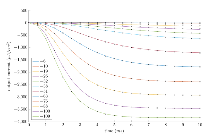
Figure 1: Outputs of the identified operator for constant input voltages from $-6mV$ to $-109mV$ (in colors). The black crosses correspond to the data samples at times $t_{0},t_{1},\dots,t_{20}$.

7 Conclusions

In this paper, we have introduced a method to incorporate bounds on the Lipschitz constant in kernel-based regularized least squares problems. As our main result, we have introduced a new class of nonexpansive kernels that induce Hilbert spaces consisting of Lipschitz continuous operators. Using regularized least squares, Lipschitz continuous operators can then be identified from data and their Lipschitz constants can be tuned by appropriate choice of the regularization parameter. We have also demonstrated how the approach enables the identification of monotone operators via the Cayley transform. The limitation of state-space modeling to achieve this objective was illustrated with a simple model of a nonlinear circuit, in particular the celebrated model of the potassium current of [Hodgkin and Huxley(1952)].

In the context of machine learning, the results of this paper are well-aligned with the objectives of [Tsuzuku et al.(2018)Tsuzuku, Sato, and Sugiyama, Fazlyab et al.(2019)Fazlyab, Robey, Hassani, Morari, and Pappas, Pauli et al.(2022)Pauli, Koch, Berberich, Kohler, and Allgöwer]. These papers focus on training input-output operators satisfying Lipschitz properties using feedforward neural network architectures. In this paper, we have argued that kernel-based models are easier to train, but more studies are needed to compare the performance and to understand the relative merits of both approaches.

In the context of systems and control, Lipschitz continuity and monotonicity are closely related to the notions of finite incremental gain and incremental passivity [Desoer and Vidyasagar(1975), van der Schaft(2017)]. These properties are the cornerstone of the analysis of feedback systems. This relation is explored in more detail in [van Waarde and Sepulchre(2021)].

References

- [Aronszajn(1950)] N. Aronszajn. Theory of reproducing kernels. Transactions of the American Mathematical Society, 68(3):337–404, 1950.
- [Bauschke and Combettes(2011)] H. H. Bauschke and P. L. Combettes. Convex Analysis and Monotone Operator Theory in Hilbert Spaces. Springer Publishing Company, Incorporated, 1st edition, 2011.
- [Bouvrie and Hamzi(2017)] J. Bouvrie and B. Hamzi. Kernel methods for the approximation of nonlinear systems. SIAM Journal on Control and Optimization, 55(4):2460–2492, 2017.
- [Caponnetto et al.(2008)Caponnetto, Micchelli, Pontil, and Ying] A. Caponnetto, C. A. Micchelli, M. Pontil, and Y. Ying. Universal multi-task kernels. Journal of Machine Learning Research, 9(52):1615–1646, 2008.
- [Carmeli et al.(2006)Carmeli, De Vito, and Toigo] C. Carmeli, E. De Vito, and A. Toigo. Vector valued reproducing kernel Hilbert spaces of integrable functions and Mercer theorem. Analysis and Applications, 4(4):377–408, 2006.
- [Combettes and Pesquet(2020)] P. L. Combettes and J.-C. Pesquet. Lipschitz certificates for layered network structures driven by averaged activation operators. SIAM Journal on Mathematics of Data Science, 2(2):529–557, 2020.
- [Desoer and Vidyasagar(1975)] C. A. Desoer and M. Vidyasagar. Feedback Systems: Input-output Properties. Electrical science series. Academic Press, 1975.
- [Dinuzzo(2015)] F. Dinuzzo. Kernels for linear time invariant system identification. SIAM Journal on Control and Optimization, 53(5):3299–3317, 2015.
- [Eykholt et al.(2018)Eykholt, Evtimov, Fernandes, Li, Rahmati, Xiao, Prakash, Kohno, and Song] K. Eykholt, I. Evtimov, E. Fernandes, B. Li, A. Rahmati, C. Xiao, A. Prakash, T. Kohno, and D. Song. Robust physical-world attacks on deep learning visual classification. In Proceedings of the IEEE/CVF Conference on Computer Vision and Pattern Recognition, pages 1625–1634, 2018.
- [Fazlyab et al.(2019)Fazlyab, Robey, Hassani, Morari, and Pappas] M. Fazlyab, A. Robey, H. Hassani, M. Morari, and G. Pappas. Efficient and accurate estimation of Lipschitz constants for deep neural networks. In Advances in Neural Information Processing Systems, volume 32, 2019.
- [Hodgkin and Huxley(1952)] A. L. Hodgkin and A. F. Huxley. A quantitative description of membrane current and its application to conduction and excitation in nerve. The Journal of Physiology, 117(4):500–544, 1952.
- [Kadri et al.(2016)Kadri, Duflos, Preux, Canu, Rakotomamonjy, and Audiffren] H. Kadri, E. Duflos, P. Preux, S. Canu, A. Rakotomamonjy, and J. Audiffren. Operator-valued kernels for learning from functional response data. Journal of Machine Learning Research, 17(20):1–54, 2016.
- [Khosravi and Smith(2019)] M. Khosravi and R. S. Smith. Kernel-based identification of positive systems. In Proceedings of the IEEE Conference on Decision and Control, pages 1740–1745, 2019.
- [Ljung et al.(2020)Ljung, Chen, and Mu] L. Ljung, T. Chen, and B. Mu. A shift in paradigm for system identification. International Journal of Control, 93(2):173–180, 2020.
- [Maddalena et al.(2021)Maddalena, Scharnhorst, and Jones] E. T. Maddalena, P. Scharnhorst, and C. N. Jones. Deterministic error bounds for kernel-based learning techniques under bounded noise. Automatica, 134, 2021.
- [Micchelli and Pontil(2004)] C. A. Micchelli and M. Pontil. Kernels for multi-task learning. Proceedings of Advances in Neural Information Processing Systems, pages 921–928, 2004.
- [Micchelli and Pontil(2005)] C. A. Micchelli and M. Pontil. On learning vector-valued functions. Neural Computation, 17(1):177–204, 2005.
- [Pauli et al.(2022)Pauli, Koch, Berberich, Kohler, and Allgöwer] P. Pauli, A. Koch, J. Berberich, P. Kohler, and F. Allgöwer. Training robust neural networks using Lipschitz bounds. IEEE Control Systems Letters, 6:121–126, 2022.
- [Pillonetto and De Nicolao(2010)] G. Pillonetto and G. De Nicolao. A new kernel-based approach for linear system identification. Automatica, 46(1):81–93, 2010.
- [Pillonetto et al.(2011)Pillonetto, Quang, and Chiuso] G. Pillonetto, M. Quang, and A. Chiuso. A new kernel-based approach for nonlinear system identification. IEEE Transactions on Automatic Control, 56(12):2825–2840, 2011.
- [Revay et al.(2020)Revay, Wang, and Manchester] M. Revay, R. Wang, and I. R. Manchester. Lipschitz bounded equilibrium networks. available online at arxiv.org/abs/2010.01732, 2020.
- [Riesz and Sz.-Nazy(1956)] F. Riesz and B. Sz.-Nazy. Functional analysis. Blackie and Son, English translation of 2nd French edition, 1956.
- [Ryu and Yin(2022)] E. K. Ryu and W. Yin. Large-Scale Convex Optimization via Monotone Operators. Cambridge University Press (to be published), 2022.
- [Scaman and Virmaux(2018)] K. Scaman and A. Virmaux. Lipschitz regularity of deep neural networks: Analysis and efficient estimation. In Proceedings of the International Conference on Neural Information Processing Systems, pages 3839–3848, 2018.
- [Schoenberg(1938)] I. J. Schoenberg. Metric spaces and completely monotone functions. Annals of Mathematics, 39(4):811–841, 1938.
- [Schölkopf and Smola(2001)] B. Schölkopf and A. J. Smola. Learning with Kernels: Support Vector Machines, Regularization, Optimization, and Beyond. MIT Press, Cambridge, MA, USA, 2001.
- [Szegedy et al.(2013)Szegedy, Zaremba, Sutskever, Bruna, Erhan, Goodfellow, and Fergus] C. Szegedy, W. Zaremba, I. Sutskever, J. Bruna, D. Erhan, I. Goodfellow, and R. Fergus. Intriguing properties of neural networks. available online at arxiv.org/abs/1312.6199, 2013.
- [Tsuzuku et al.(2018)Tsuzuku, Sato, and Sugiyama] Y. Tsuzuku, I. Sato, and M. Sugiyama. Lipschitz-margin training: Scalable certification of perturbation invariance for deep neural networks. In Advances in Neural Information Processing Systems, volume 31, 2018.
- [van der Schaft(2017)] A. van der Schaft. L2-Gain and Passivity Techniques in Nonlinear Control. Springer, 3rd edition, 2017.
- [van Waarde and Sepulchre(2021)] H. J. van Waarde and R. Sepulchre. Kernel-based models for system analysis. available online at arxiv.org/abs/2110.11735, 2021.