Learning Connectivity with Graph Convolutional Networks for Skeleton-based Action Recognition

Abstract

Learning graph convolutional networks (GCNs) is an emerging field which aims at generalizing convolutional operations to arbitrary non-regular domains. In particular, GCNs operating on spatial domains show superior performances compared to spectral ones, however their success is highly dependent on how the topology of input graphs is defined.
In this paper, we introduce a novel framework for graph convolutional networks that learns the topological properties of graphs. The design principle of our method is based on the optimization of a constrained objective function which learns not only the usual convolutional parameters in GCNs but also a transformation basis that conveys the most relevant topological relationships in these graphs. Experiments conducted on the challenging task of skeleton-based action recognition shows the superiority of the proposed method compared to handcrafted graph design as well as the related work.

1 Introduction

Deep learning is currently witnessing a major interest in computer vision and neighboring fields [48]. Its principle consists in learning mapping functions, as multi-layered convolutional or recurrent neural networks, whose inputs correspond to different stimulus (images, videos, etc.) and outputs to their classification and regression. Early deep learning architectures, including AlexNet [49] and other networks [50, 52, 53, 54, 55, 57, 58, 59, 61, 63, 64, 62, 66, 68, 69, 70, 71, 72, 74, 75, 77, 76, 78, 79, 73, 67, 65, 80], were initially dedicated to vectorial data such as images [49, 52]. However, data sitting on top of irregular domains (including graphs) require extending deep learning to non-vectorial data [83, 84, 85, 86]. These extensions, widely popularized as graph neural networks (GNNs), are currently emerging for different use-cases and applications [105]. Two major families of GNNs exist in the literature; spectral and spatial. Spectral methods [83, 84, 82, 86, 87, 88, 89, 81, 85] achieve convolution by projecting the signal of a given graph onto a Fourier basis (as the spectral decomposition of the graph Laplacian) prior to its convolution in the spectral domain using the hadamard (entrywise) product, and then back-projecting the resulting convoluted signal in the input domain using the inverse of the Fourier transform [118]. Whilst spectral convolution is well defined, it requires solving a cumbersome eigen-decomposition of the Laplacian. Besides, the resulting Fourier basis is graph-dependent and non-transferable to general and highly irregular graph structures [105]. Another category of GNNs, dubbed as spatial [99, 97, 100, 101, 103], has also emerged and seeks to achieve convolutions directly in the input domain without any preliminary step of spectral decomposition. Its general principle consists in aggregating node representations before applying convolution to the vectorized node aggregates [107, 108, 106, 103, 105, 104]. This second category of methods is deemed computationally more efficient and also more effective compared to spectral ones; however, its success is reliant on the aggregate operators which in turn depend on the topology of input graphs.
Graph topology is usually defined with one or multiple adjacency matrices (or equivalently their Laplacian operators) that capture connectivity in these graphs as well as their differential properties. Most of the existing GNN architectures rely on predetermined graph structures which dependent on the properties of the underlying applications [119, 120, 121] (e.g., node-to-node relationships in social networks [101], edges in 3D modeling [20, 19, 22, 23, 25], protein connectivity in biological systems [115, 116], etc.) whilst other methods handcraft graph connections by modeling similarities between nodes [40]. However, connections (either intrinsically available or handcrafted) are powerless to optimally capture all the relationships between nodes as their setting is oblivious to the targeted applications. For instance, node-to-node relationships, in human skeletons, capture the intrinsic anthropometric characteristics of individuals (useful for their identification) while other connections, yet to infer, are necessary for recognizing their dynamics and actions (See Fig. 2). Put differently, depending on the task at hand, connectivity should be appropriately learned by including not only the existing intrinsic links between nodes in graphs but also their extrinsic (inferred) relationships.
In this paper, we introduce a novel framework that learns convolutional filters on graphs together with their topological properties. The latter are modeled through matrix operators that capture multiple aggregates on graphs. Learning these topological properties relies on a constrained cross-entropy loss whose solution corresponds to the learned entries of these matrix operators. We consider different constraints (including stochasticity, orthogonality and symmetry) acting as regularizers which reduce the space of possible solutions and the risk of overfitting. Stochasticity implements random walk Laplacians while orthogonality models multiple aggregation operators with non-overlapping supports; it also avoids redundancy and oversizing the learned GNNs with useless parameters. Finally, symmetry reduces further the number of training parameters and allows learning positive semi-definite matrix operators. We also consider different reparametrizations, particularly crispmax, that implement orthogonality while being highly effective as shown later in experiments.

2 Related work

Without any a priori knowledge, graph inference (a.k.a graph design) is ill-posed and NP-hard [129, 130, 131]. Most of the existing solutions rely on constraints (including similarity, smoothness, sparsity, band-limitedness, etc. [127, 3, 4, 12, 9, 14, 11, 5, 6, 8, 15]) which have been adapted for a better conditioning of graph design [16, 18]. From the machine learning point-of-view and particularly in GNNs, early methods [97, 43] rely on handcrafted or predetermined graphs that model node-to-node relationships using similarities or the inherent properties of the targeted applications [102, 29, 41]. These relationships define operators (with adjacency matrices or Laplacians) that aggregate the neighbors of nodes before applying convolutions on the resulting aggregates. Existing operators include the power series of the adjacency matrices [133] (a.k.a power maps) and also the recursive Chebyshev polynomial which provides an orthogonal Laplacian basis [40]. However, in spite of being relatively effective, the potential of these handcrafted operators is not fully explored as their design is either rigid or agnostic to the tasks at hand or achieved using the tedious cross validation. More recent alternatives seek to define graph topology that best fits a given classification or regression problem [90, 91, 92, 94, 95, 96, 89, 88]. For instance, authors in [95] propose a GNN for semi-supervised classification tasks that learns graph topology with sparse structure given a cloud of points; node-to-node connections are modeled with a joint probability distribution on Bernoulli random variables whose parameters are found using bi-level optimization. A computationally more efficient variant of this method is introduced in [96] using a weighted cosine similarity and edge thresholding.
Other solutions make improvement over the original GNNs in [43] by exploiting symmetric matrices; for instance, the adaptive graph convolutional network in [88] discovers hidden structural relations (unspecified in the original graphs), using a so-called residual graph adjacency matrix by learning a distance function over nodes. The work in [89] introduces a dual architecture with two parallel graph convolutional layers sharing the same parameters. This method considers a normalized adjacency matrix and a positive pointwise mutual information matrix in order to capture node co-occurrences through random walks sampled from a graph. The difference of our contribution, w.r.t this related work, resides in multiple aspects; on the one hand, in contrast to many existing methods (e.g., [133] which consider a single adjacency matrix shared through power series), the matrix operators designed in our contribution are non-parametrically learned and this provides more flexibility to our design. On the other hand, constraining these matrices (through stochasticity, orthogonality and symmetry) provides us with an effective regularization that mitigates overfitting as corroborated later in experiments.

3 Spatial graph convolutional networks

Let ${\cal S}=\{{\cal G}_{i}=({\cal V}_{i},{\cal E}_{i})\}_{i}$ denote a collection of graphs with ${\cal V}_{i}$, ${\cal E}_{i}$ being respectively the nodes and the edges of ${\cal G}_{i}$. Each graph ${\cal G}_{i}$ (denoted for short as ${\cal G}=({\cal V},{\cal E})$) is endowed with a graph signal $\{\psi(u)\in\mathbb{R}^{s}:\ u\in{\cal V}\}$ and associated with an adjacency matrix ${\bf A}$ with each entry ${\bf A}_{uu^{\prime}}>0$ iff $(u,u^{\prime})\in{\cal E}$ and $0$ otherwise. Graph convolutional networks (GCNs) return both the representation and the classification of ${\cal G}$ by learning $K$ filters ${\cal F}=\{g_{\theta}\}_{\theta=1}^{K}$; each filter $g_{\theta}=({\cal V}_{\theta},{\cal E}_{\theta})$, also referred to as graphlet, corresponds to a graph with a small number of nodes and edges, i.e., $|{\cal V}_{\theta}|\ll|{\cal V}|$ and $|{\cal E}_{\theta}|\ll|{\cal E}|$. This filter $g_{\theta}$ defines a convolution at a given node $u\in{\cal V}$ of ${\cal G}$ as

$$({\cal G}\star g_{\theta})_{u}=f\bigg{(}\frac{1}{|{\cal V}_{\theta}|}\sum_{u^{\prime}\in{\cal N}_{r}(u),v\in{\cal V}_{\theta}}\big{\langle}\psi(u^{\prime}),\psi(v)\big{\rangle}\bigg{)},$$ (1)

being $f$ a nonlinear activation, ${\cal N}_{r}(u)$ the $r$-hop neighbors of $u$ and $\langle.,.\rangle:\mathbb{R}^{s}\times\mathbb{R}^{s}\rightarrow\mathbb{R}$ the inner product. This graph convolution — similar to the convolution kernel [1] — bypasses the ill-posedness of the spatial support around $u$ due to arbitrary degrees and node permutations in ${\cal N}_{r}(u)$; since the input of $f$ is defined as the sum of all of the inner products between all of the possible signal pairs taken from $\psi({\cal N}_{r}(u))\times\psi({\cal V}_{\theta})$, its evaluation does not require any hard-alignment between these pairs and it is thereby agnostic to any arbitrary automorphism in ${\cal G}$ and $g_{\theta}$.
Considering $w_{\theta}=\frac{1}{|{\cal V}_{\theta}|}\sum_{v\in{\cal V}_{\theta}}\psi(v)$ as the aggregate of the graph signal in ${\cal V}_{\theta}$, Eq. (1) reduces to

$$({\cal G}\star g_{\theta})_{u}=f\bigg{(}\bigg{\langle}\sum_{u^{\prime}}{\bf A}^{{\!(r)}}_{uu^{\prime}}.\psi(u^{\prime}),w_{\theta}\bigg{\rangle}\bigg{)},$$ (2)

with ${{\bf A}^{{\!(r)}}_{\phantom{+}}}$ being the $r$-hop adjacency matrix of ${\cal G}$. From this definition, knowing the parameters of the aggregate $w_{\theta}$ is sufficient in order to well define spatial convolutions on graphs. Besides, each aggregate filter $w_{\theta}$ has less parameters, and its learning is less subject to overfitting, compared to the non-aggregate filter $g_{\theta}$ especially when the latter is stationary so the parameters of $w_{\theta}$ could be shared through different locations (nodes) of ${\cal G}$. Using Eq. (2), the extension of convolution to $K$-filters and $|{\cal V}|$ nodes can be written as

$$({\cal G}\star{\cal F})_{\cal V}=f\big{(}{{\bf A}^{{\!(r)}}_{\phantom{+}}}\ {\bf U}^{\top}\ {\bf W}\big{)},$$ (3)

here ^⊤ is the matrix transpose operator, ${\bf U}\in\mathbb{R}^{s\times n}$ is the graph signal (with $n=|{\cal V}|$), ${\bf W}\in\mathbb{R}^{s\times C}$ is the matrix of convolutional parameters corresponding to the $C$ channels (filters) and $f(.)$ is now applied entrywise. In Eq. 3, the input signal ${\bf U}$ is projected using the adjacency matrix ${\bf A}$ and this provides for each node $u$, the aggregate set of its neighbors. Taking powers of ${\bf A}$ (i.e., ${\bf A}^{\!(r)}$, with $r>1$) makes it possible to capture the $r$-hop neighbor aggregates in ${\cal V}$ and thereby to model larger extents and more influencing contexts. When the adjacency matrix ${\bf A}$ is common to all graphs, entries of ${\bf A}$ could be handcrafted or learned so Eq. (3) implements a convolutional network with two layers; the first one aggregates signals in ${\cal N}_{r}({\cal V})$ by multiplying ${\bf U}$ with ${\bf A}^{\!(r)}$ while the second layer achieves convolution by multiplying the resulting aggregate signals with the $C$ filters in ${\bf W}$.

4 Learning connectivity in GCNs

In the sequel of this paper, we rewrite the aforementioned adjacency matrices as $\{{\bf A}_{k}\}_{k}$; the latter will also be referred to as context matrices. Following Eq. 3, the term ${\bf A}_{k}{\bf U}^{\top}$ acts as a feature extractor that collects different statistics including means and variances of node contexts; indeed, when ${\bf A}_{k}$ is column-stochastic, ${\bf A}_{k}{\bf U}^{\top}$ models expectations $\{\mathbb{E}(\psi({\cal N}_{r}(u)))\}_{u}$, and if one considers ${\bf I}-{\bf A}_{k}$ instead of ${\bf A}_{k}$, then $({\bf I}-{\bf A}_{k})\ {\bf U}^{\top}$ captures (up to a squared power) statistical variances $\{\psi(u)-\mathbb{E}(\psi({\cal N}_{r}(u)))\}_{u}$. Therefore, $\{{\bf A}_{k}\}_{k}$ constitutes a transformation basis (possibly overcomplete) which allows extracting first and possibly higher order statistics of graph signals before convolution. One may also design this basis to make it orthogonal, by constraining the learned matrices $\{{\bf A}_{k}\}_{k}$ to be cycle and loop-free (such as trees), and consider the power map ${\bf A}_{k}={\bf A}^{\!(k)}$, so the basis $\{{\bf A}_{k}\}_{k}$ becomes necessarily orthogonal (see later section 5.2). The latter property — which allows learning compact and complementary convolutional filters — is extended to unconstrained graph structures as shown subsequently.
Considering ${E}$ as the cross entropy loss associated to a given classification task and ${\bf vec}(\{{\bf A}_{k}\}_{k})$ as a vectorization that appends all the entries of $\{{\bf A}_{k}\}_{k}$ following any arbitrary order, we turn the design of $\{{\bf A}_{k}\}_{k}$ as a part of GCN learning. As the derivatives of ${E}$ w.r.t different layers of the GCN are known (including the output of convolutional layer in Eq. 3), one may use the chain rule in order to derive the gradient $\frac{\partial{E}}{\partial{\bf vec}(\{{\bf A}_{k}\}_{k})}$ and hence update the entries of $\{{\bf A}_{k}\}_{k}$ using stochastic gradient descent (SGD). In this section, we upgrade SGD by learning both the convolutional parameters of GCNs together with the matrices $\{{\bf A}_{k}\}_{k}$ while implementing orthogonality, stochasticity and symmetry. As shown subsequently, orthogonality allows us to design $\{{\bf A}_{k}\}_{k}$ with a minimum number of parameters, stochasticity normalizes nodes by their degrees and allows learning normalized random walk Laplacians, while symmetry reduces further the number of training parameters by constraining the upper and the lower triangular parts of the learned $\{{\bf A}_{k}\}_{k}$ to share the same parameters, and also the underlying learned random walk Laplacians to be positive semi-definite.

4.1 Stochasticity

In this subsection, we rewrite ${\bf A}_{k}$ for short as ${\bf A}$. Stochasticity of a given matrix ${\bf A}$ ensures that all of its entries are positive and each column sums to one; i.e. the matrix ${\bf A}$ models a Markov chain whose entry ${\bf A}_{ij}$ provides the probability of transition from one node $u_{j}$ to $u_{i}$ in ${\cal G}$. In other words, the matrix ${\bf A}$ captures probabilistically how reachable is the set of neighbors (context) of a given node $u_{j}$. Taking powers of a stochastic matrix ${\bf A}$ provides the probability of transition in multiple steps and these powers also preserve stochasticity. This property also implements normalized random walk Laplacian operators which are valuable in the evaluation of weighted means and variances in Eq. 3 using a standard feed-forward network; otherwise, one has to consider a normalization layer (with extra parameters), especially on graphs with heterogeneous degrees in order to reduce the covariate shift and distribute the transition probability evenly through nodes before achieving convolutions. Hence, stochasticity acts as a regularizer that reduces the complexity (number of layers and parameters) in the learned GCN and thereby the risk of overfitting.
Stochasticity requires adding equality and inequality constraints in SGD, i.e., ${\bf A}_{ij}\in[0,1]$ and $\sum_{q}{\bf A}_{qj}=1$. In order to implement these constraints, we consider a reparametrization of the learned matrices, as ${\bf A}_{ij}=h(\hat{{\bf A}}_{ij})/{\sum_{q}h(\hat{{\bf A}}_{qj})}$, with $h:\mathbb{R}\rightarrow\mathbb{R}^{+}$ being strictly monotonic and this allows a free setting of the matrix $\hat{{\bf A}}$ during optimization while guaranteeing ${\bf A}_{ij}\in[0,1]$ and $\sum_{q}{\bf A}_{qj}=1$. During backpropagation, the gradient of the loss ${E}$ (now w.r.t $\hat{{\bf A}}$) is updated using the chain rule as

$$\begin{array}[]{lll}\displaystyle\frac{\partial{E}}{\partial\hat{{\bf A}}_{ij}}&=&\displaystyle\sum_{p}\frac{\partial{E}}{\partial{\bf A}_{pj}}.\frac{\partial{\bf A}_{pj}}{\partial\hat{{\bf A}}_{ij}}\\ &&\textrm{with}\displaystyle\ \ \ \frac{\partial{\bf A}_{pj}}{\partial\hat{{\bf A}}_{ij}}=\frac{h^{\prime}(\hat{{\bf A}}_{pj})}{\sum_{q}h(\hat{{\bf A}}_{qj})}.(\delta_{pi}-{\bf A}_{pj}),\par\end{array}$$ (4)

and $\delta_{pi}=1_{\{p=i\}}$. In practice $h$ is set to $\exp$ and the original gradient $\big{[}\frac{\partial{E}}{\partial{{\bf A}}_{pj}}\big{]}_{p=1}^{n}$ is obtained from layerwise gradient back propagation (as already integrated in standard deep learning tools including PyTorch). Hence the new gradient (w.r.t $\hat{{\bf A}}$) is obtained by multiplying the original one by the Jacobian ${\bf J}_{\textrm{stc}}=\big{[}\frac{\partial{{\bf A}}_{pj}}{\partial{\hat{{\bf A}}}_{ij}}\big{]}_{p,i=1}^{n}$ which merely reduces to $[{{\bf A}}_{ij}.(\delta_{pi}-{\bf A}_{pj})]_{p,i}$ when $h(.)=\exp(.)$.

4.2 Orthogonality

Learning multiple matrices $\{{\bf A}_{k}\}_{k}$ allows us to capture different contexts and graph topologies when achieving aggregation and convolution, and this enhances the discrimination power of the learned GCN representation as shown later in experiments. With multiple matrices $\{{\bf A}_{k}\}_{k}$ (and associated convolutional filter parameters $\{{\bf W}_{k}\}_{k}$), Eq. 3 is updated as

$$({\cal G}\star{\cal F})_{\cal V}=f\bigg{(}\sum_{k=1}^{K}{\bf A}_{k}{\bf U}^{\top}{\bf W}_{k}\bigg{)}.$$ (5)

If aggregation produces, for a given $u\in{\cal V}$, linearly dependent vectors ${\cal X}_{u}=\{\sum_{u^{\prime}}{\bf A}_{kuu^{\prime}}.\psi(u^{\prime})\}_{k}$, then convolution will also generate linearly dependent representations with an overestimated number of training parameters in the null space of ${\cal X}_{u}$. Besides, matrices $\{{\bf A}_{1},\dots,{\bf A}_{K}\}$ used for aggregation, may also generate overlapping and redundant contexts.
Provided that $\{\psi(u^{\prime})\}_{u^{\prime}\in{\cal N}_{r}(u)}$ are linearly independent, the sufficient condition that makes vectors in ${\cal X}_{u}$ linearly independent reduces to constraining $({\bf A}_{kuu^{\prime}})_{k,u^{\prime}}$ to lie on the Stiefel manifold (see for instance [123, 124, 126]) defined as $V_{K}(\mathbb{R}^{n})=\{{\bf M}\in\mathbb{R}^{K\times n}:{\bf M}\,{\bf M}^{\top}={\bf I}_{K}\}$ (with ${\bf I}_{K}$ being the $K\times K$ identity matrix) which thereby guarantees orthonormality and minimality of $\{{\bf A}_{1},\dots,{\bf A}_{K}\}$. A less compelling condition is orthogonality, i.e., $\langle{\bf A}_{k},{\bf A}_{k^{\prime}}\rangle_{F}=0$ and ${\bf A}_{k}\geq{\bf 0}_{n}$, ${\bf A}_{k^{\prime}}\geq{\bf 0}_{n}$, $\forall k\neq k^{\prime}$ — with $\langle,\rangle_{F}$ being the Hilbert-Schmidt (or Frobenius) inner product defined as $\langle{\bf A}_{k},{\bf A}_{k^{\prime}}\rangle_{F}={\bf Tr}({\bf A}_{k}^{\top}{\bf A}_{k^{\prime}})$ — and this equates ${\bf A}_{k}\odot{\bf A}_{k^{\prime}}={\bf 0}_{n}$, $\forall k\neq k^{\prime}$ with $\odot$ denoting the entrywise hadamard product and ${\bf 0}_{n}$ the $n\times n$ null matrix.

4.2.1 Problem statement

Considering the cross entropy loss $E$, the matrix operators $\{{\bf A}_{k}\}_{k}$ (together with the convolutional filter parameters ${\bf W}=\{{\bf W}_{k}\}_{k}$) are learned as

$$\begin{array}[]{lll}\displaystyle{\displaystyle\min}_{\{{\bf A}_{k}\}_{k},{\bf W}}&\displaystyle E\big{(}{\bf A}_{1},\dots,{\bf A}_{K};{\bf W}\big{)}&\\ &&\\ \displaystyle{\textrm{s.t.}}&{\bf A}_{k}\odot{\bf A}_{k}>{\bf 0}_{n}&\\ &{\bf A}_{k}\odot{\bf A}_{k^{\prime}}={\bf 0}_{n}&\forall k,k^{\prime}\neq k.\end{array}$$ (6)

A natural approach to solve this problem is to iteratively and alternately minimize over one matrix while keeping all the others fixed. However — and besides the non-convexity of the loss — the feasible set formed by these $O(K^{2})$ bi-linear constraints is not convex w.r.t $\{{\bf A}_{k}\}_{k}$. Moreover, this iterative procedure is computationally expensive as it requires solving multiple instances of constrained projected gradient descent and the number of necessary iterations to reach convergence is large in practice. All these issues make solving this problem challenging and computationally intractable even for reasonable values of $K$ and $n$. In what follows, we consider an alternative, dubbed as crispmax, that makes the design of orthogonality substantially more tractable and also effective.

4.2.2 Crispmax

We investigate a workaround that optimizes these matrices while guaranteeing their orthogonality as a part of the optimization process. Considering $\exp(\gamma\hat{{\bf A}}_{k})\oslash(\sum_{r=1}^{K}\exp(\gamma\hat{{\bf A}}_{r}))$ as a softmax reparametrization of ${\bf A}_{k}$, with $\oslash$ being the entrywise hadamard division and $\{\hat{{\bf A}}_{k}\}_{k}$ free parameters in $\mathbb{R}^{n\times n}$, it becomes possible to implement orthogonality by choosing large values of $\gamma$ in order to make this softmax crisp; i.e., only one entry ${\bf A}_{kij}\gg 0$ while all others $\{{\bf A}_{k^{\prime}ij}\}_{k^{\prime}\neq k}$ vanishing thereby leading to ${\bf A}_{k}\odot{\bf A}_{k^{\prime}}={\bf 0}_{n}$, $\forall k,k^{\prime}\neq k$. By plugging this crispmax reparametrization into Eq. 6, the gradient of the loss ${E}$ (now w.r.t $\{\hat{{\bf A}}_{k}\}_{k}$) is updated using the chain rule as

$$\begin{array}[]{lll}\displaystyle&\displaystyle\frac{\partial{E}}{\partial{\bf vec}(\{\hat{{\bf A}}_{k}\}_{k})}&=\displaystyle{\bf J}_{\textrm{orth}}.\frac{\partial{E}}{\partial{\bf vec}({\{{{\bf A}}_{k}\}_{k}})},\end{array}$$ (7)

with each entry $({\bf i},{\bf j})=(kij,k^{\prime}i^{\prime}j^{\prime})$ of the Jacobian ${\bf J}_{\textrm{orth}}$ being

$$\begin{array}[]{lll}&\displaystyle\left\{\begin{array}[]{ll}\gamma{{\bf A}}_{kij}.(1-{\bf A}_{kij})&{\footnotesize\textrm{if}\ k=k^{\prime},i=i^{\prime},j=j^{\prime}}\\ -\gamma{{\bf A}}_{kij}.{\bf A}_{k^{\prime}ij}&{\small\textrm{if}\ k\neq k^{\prime},i=i^{\prime},j=j^{\prime}}\\ 0&\textrm{\small otherwise,}\end{array}\right.\end{array}$$ (8)

here $\frac{\partial{E}}{\partial{\bf vec}({\{{{\bf A}}_{k}\}_{k}})}$ is obtained from layerwise gradient backpropagation. Note that the aforementioned Jacobian is extremely sparse and efficient to evaluate as only $Kn^{2}$ entries are non-zeros (among the $K^{2}n^{4}$ possible entries). However, with this reparametrization, large values of $\gamma$ may lead to numerical instability when evaluating the exponential. We circumvent this instability by choosing $\gamma$ that satisfies $\epsilon$-orthogonality: a surrogate property defined subsequently.

Definition 1 ($\epsilon$-orthogonality)

A basis $\{{\bf A}_{1},\dots,{\bf A}_{K}\}$ is $\epsilon$-orthogonal if $\ \forall k,k^{\prime}\neq k$,

$${\bf A}_{k}\odot{\bf A}_{k^{\prime}}\leq\epsilon\ \mathds{1}_{n},$$

with $\mathds{1}_{n}$ being the $n\times n$ unitary matrix.

Considering the above definition, (nonzero) matrices belonging to an $\epsilon$-orthogonal basis are linearly independent w.r.t $\langle.,.\rangle_{F}$ (provided that $\gamma$ is sufficiently large) and hence this basis is also minimal. The following proposition provides a tight lower bound on $\gamma$ that satisfies $\epsilon$-orthogonality.

Proposition 1 ($\epsilon$-orthogonality bound)

Consider $\{{\bf A}_{kij}\}_{ij}$ as the entries of the crispmax reparametrized matrix ${\bf A}_{k}$ defined as $\exp(\gamma\hat{{\bf A}}_{k})\oslash\big{(}\sum_{r=1}^{K}\exp(\gamma\hat{{\bf A}}_{r})\big{)}$. Provided that $\exists\delta>0:$ $\forall i,j,\ell^{\prime}$, $\exists!\ell$, $\hat{{\bf A}}_{\ell ij}\geq\hat{{\bf A}}_{\ell^{\prime}ij}+\delta$ (with $\ell^{\prime}\neq\ell$) and if $\gamma$ is at least

$$\frac{1}{\delta}\ln\bigg{(}\frac{K\sqrt{(1-2\epsilon)}}{1-\sqrt{(1-2\epsilon)}}+1\bigg{)}$$

then $\{{\bf A}_{1},\dots,{\bf A}_{K}\}$ is $\epsilon$-orthogonal.

Proof 1

For any entry $i,j$, one may find $\ell$, $\ell^{\prime}$ in $\{1,\dots,K\}$ (with $\ell\neq\ell^{\prime}$) s.t. $({\bf A}_{k}\odot{\bf A}_{k^{\prime}})_{ij}$

$$\begin{array}[]{lll}\displaystyle&\leq&\displaystyle({\bf A}_{\ell}\odot{\bf A}_{\ell^{\prime}})_{ij}\\ &&\\ &=&\frac{1}{2}({\bf A}_{\ell ij}^{2}+{\bf A}_{\ell^{\prime}ij}^{2})-\frac{1}{2}({\bf A}_{\ell ij}-{\bf A}_{\ell^{\prime}ij})^{2}\\ &&\\ \displaystyle&\leq&\frac{1}{2}-\frac{1}{2}({\bf A}_{\ell ij}-{\bf A}_{\ell^{\prime}ij})^{2}\\ \displaystyle&=&\frac{1}{2}-\frac{1}{2}\bigg{(}\displaystyle\frac{\exp(\gamma\hat{{\bf A}}_{\ell ij})-\exp(\gamma\hat{{\bf A}}_{\ell^{\prime}ij})}{\exp(\gamma\hat{{\bf A}}_{\ell ij})+\exp(\gamma\hat{{\bf A}}_{\ell^{\prime}ij})+\sum_{r=3}^{K}\exp(\gamma\hat{{\bf A}}_{rij})}\bigg{)}^{2}\\ &&\\ \displaystyle&\leq&\frac{1}{2}-\frac{1}{2}\bigg{(}\displaystyle\frac{\exp(\gamma\hat{{\bf A}}_{\ell ij})-\exp(\gamma\hat{{\bf A}}_{\ell^{\prime}ij})}{\exp(\gamma\hat{{\bf A}}_{\ell ij})+(K-1)\exp(\gamma\hat{{\bf A}}_{\ell^{\prime}ij})}\bigg{)}^{2}\\ &&\\ \displaystyle&\leq&\frac{1}{2}-\frac{1}{2}\bigg{(}\displaystyle\frac{1}{1+\frac{K}{\exp(\gamma\delta)-1}}\bigg{)}^{2}.\end{array}$$

The sufficient condition is to choose $\gamma$ such as

$$\frac{1}{2}-\frac{1}{2}\bigg{[}\displaystyle\frac{1}{1+\frac{K}{\exp(\gamma\delta)-1}}\bigg{]}^{2}\leq\epsilon\implies\displaystyle\gamma\geq\displaystyle\frac{1}{\delta}\ln\bigg{(}\frac{K\sqrt{(1-2\epsilon)}}{1-\sqrt{(1-2\epsilon)}}+1\bigg{)}.$$

$\blacksquare$

Following the above proposition, setting $\gamma$ to the above lower bound guarantees $\epsilon$-orthogonality; for instance, when $K=2$, $\delta=0.01$ and provided that $\gamma\geq 530$, one may obtain $0.01$-orthogonality which is almost a strict orthogonality. This property is satisfied as long as one slightly disrupts the entries of $\{\hat{{\bf A}}_{k}\}_{k}$ with random noise during SGD training. However, this may still lead to another limitation; precisely, bad local minima are observed due to an early convergence to crisp adjacency matrices. We prevent this by steadily annealing the temperature $1/\gamma$ of the softmax through epochs of SGD (using $\frac{\gamma.\textrm{epoch}}{\textrm{max\_epochs}}$ instead of $\gamma$) in order to make optimization focusing first on the loss, and then as optimization evolves, temperature cools down and allows reaching the aforementioned lower bound (thereby crispmax) and $\epsilon$-orthogonality at convergence.

4.3 Symmetry & Combination

Symmetry is obtained using weight sharing, i.e., by constraining the upper and the lower triangular parts of the matrices $\{{\bf A}_{k}\}_{k}$ to share the same entries. This is guaranteed by considering the reparametrization of each matrix as ${\bf A}_{k}=\frac{1}{2}(\hat{{\bf A}}_{k}+\hat{{\bf A}}_{k}^{\top})$ with $\hat{{\bf A}}_{k}$ being a free matrix. Starting from symmetric $\{{\bf A}_{k}\}_{k}$, weight sharing is maintained through SGD by tying pairwise symmetric entries of the gradient $\frac{\partial{E}}{\partial{\bf vec}(\{\hat{{\bf A}}_{k}\}_{k})}$ and this is equivalently obtained by multiplying the original gradient $\frac{\partial{E}}{\partial{\bf vec}(\{{{\bf A}}_{k}\}_{k})}$ by the Jacobian ${\bf J}_{\textrm{sym}}=\frac{1}{2}\big{[}1_{\{k=k^{\prime}\}}.1_{\{(i=i^{\prime},j=j^{\prime})\vee(i=j^{\prime},j=i^{\prime})\}}\big{]}_{ijk,i^{\prime}j^{\prime}k^{\prime}}$ which is again extremely sparse and highly efficient to evaluate.
One may combine symmetry with all the aforementioned constraints by multiplying the underlying Jacobians, so the final gradient is obtained by multiplying the original one as

$$\frac{\partial{E}}{\partial{\bf vec}(\{\hat{{\bf A}}_{k}\}_{k})}=\displaystyle{\bf J}_{\textrm{(sym or stc)}}.{\bf J}_{\textrm{orth}}.\frac{\partial{E}}{\partial{\bf vec}(\{{{\bf A}}_{k}\}_{k})}.$$ (9)

Since all the Jacobians are sparse, their product provides an extremely sparse Jacobian. This order of application is strict, as orthogonality sustains after the two other operations, while the converse is not necessarily guaranteed at the end of the optimization process. Note that symmetry could be combined with orthogonality but not with stochasticity as the latter may undo the effect of symmetry if applied subsequently; the converse is also true.

5 Experiments

We evaluate the performance of our GCN learning framework on the challenging task of action recognition [110, 111, 112, 114], using the SBU kinect dataset [19]. The latter is an interaction dataset acquired using the Microsoft kinect sensor; it includes in total 282 video sequences belonging to $8$ categories: “approaching”, “departing”, “pushing”, “kicking”, “punching”, “exchanging objects”, “hugging”, and “hand shaking” with variable duration, viewpoint changes and interacting individuals (see examples in Fig. 1). In all these experiments, we use the same evaluation protocol as the one suggested in [19] (i.e., train-test split) and we report the average accuracy over all the classes of actions.

5.1 Video skeleton description

Given a video ${\cal V}$ in SBU as a sequence of skeletons, each keypoint in these skeletons defines a labeled trajectory through successive frames (see Fig. 1). Considering a finite collection of trajectories $\{v_{j}\}_{j}$ in ${\cal V}$, we process each trajectory using temporal chunking: first we split the total duration of a video into $M$ equally-sized temporal chunks ($M=8$ in practice), then we assign the keypoint coordinates of a given trajectory $v_{j}$ to the $M$ chunks (depending on their time stamps) prior to concatenate the averages of these chunks and this produces the description of $v_{j}$ (again denoted as $\psi(v_{j})\in\mathbb{R}^{s}$ with $s=3\times M$) and $\{\psi(v_{j})\}_{j}$ constitutes the raw description of nodes in a given video ${\cal V}$. Note that two trajectories $v_{j}$ and $v_{k}$, with similar keypoint coordinates but arranged differently in time, will be considered as very different when using temporal chunking. Note also that beside being compact and discriminant, this temporal chunking gathers advantages – while discarding drawbacks – of two widely used families of techniques mainly global averaging techniques (invariant but less discriminant) and frame resampling techniques (discriminant but less invariant). Put differently, temporal chunking produces discriminant raw descriptions that preserve the temporal structure of trajectories while being frame-rate and duration agnostic.

Figure 1: This figure shows the whole keypoint tracking and description process.

5.2 Setting & Performances

We trained the GCN networks end-to-end for 3,000 epochs with a batch size equal to $200$, a momentum of $0.9$ and a learning rate (denoted as $\nu(t)$) inversely proportional to the speed of change of the cross entropy loss used to train our networks; when this speed increases (resp. decreases), $\nu(t)$ decreases as $\nu(t)\leftarrow\nu(t-1)\times 0.99$ (resp. increases as $\nu(t)\leftarrow\nu(t-1)/0.99$). All these experiments are run on a GeForce GTX 1070 GPU device (with 8 GB memory) and no data augmentation is achieved.

Baselines. We compare the performances of our GCN against two power map baselines. The latter, closely related to our contribution, is given as ${\bf A}_{k}={\bf A}^{\!(k)}$ with ${\bf A}^{\!(k)}={\bf A}^{\!(k-1)}{\bf A}$, ${\bf A}^{\!(0)}={\bf I}$ and this defines nested supports for convolutions. Two variants of this baseline are also considered in our experiments

• Handcrafted. All the matrices $\{{\bf A}_{k}\}_{k}$ are evaluated upon a handcrafted adjacency matrix ${\bf A}$ (set using the original skeleton). In this setting, orthogonality is obtained when only a subset of edges in ${\cal G}$ (or equivalently in the adjacency matrix ${\bf A}$) are kept; this subset corresponds to edges of a spanning tree of ${\bf A}$ obtained using Kruskal [134]. With this initial setting of ${\bf A}$, orthogonality is maintained through $\{{\bf A}_{k}\}_{k}$ by updating only the nonzero entries of these matrices. Symmetry (resp. stochasticity) is obtained by taking $\frac{1}{2}({\bf A}+{\bf A}^{\top})$ (resp. ${\bf A}{\bf D}({\bf A})^{-1}$ with ${\bf D}({\bf A})$ being the degree matrix of ${\bf A}$) instead of ${\bf A}$ so all the resulting matrices $\{{\bf A}_{k}\}_{k}$ will preserve these two properties.

• Learned. In this variant, all the unmasked entries of the matrices $\{{\bf A}_{k}\}_{k}$ are learned. In contrast to the handcrafted setting, orthogonality is obtained as a part of the optimization process (as already discussed in section 4.2), so the original matrix ${\bf A}$ does not necessarily correspond to a spanning tree. Similarly, stochasticity and symmetry are implemented as a part of the optimization process; nonetheless, symmetry is structural, i.e., it is obtained by further constraining the structure of the masks, defining the nonzero entries of $\{{\bf A}_{k}\}_{k}$, to be symmetric.

		none	sym	orth	stc	sym+orth	orth+stc	Mean
HPM.	$K=1$	89.2308	92.3077	–	89.2308	–	–	90.2564
	$K=4$	87.6923	89.2308	89.2308	87.6923	90.7692	92.3077	89.4872
	$K=8$	90.7692	95.3846	92.3077	90.7692	92.3077	92.3077	92.3077
	Mean	89.2308	92.3077	90.7692	89.2308	91.5384	92.3077	90.7692
LPM.	$K=1$	92.3077	87.6923	–	95.3846	–	–	91.7949
	$K=4$	92.3077	92.3077	93.8462	95.3846	90.7692	96.9231	93.5897
	$K=8$	95.3846	90.7692	87.6923	93.8462	93.8462	92.3077	92.3077
	Mean	93.3333	90.2564	90.7692	94.8718	92.3077	94.6154	92.7180
Our	$K=1$	95.3846	93.8462	–	95.3846	–	–	94.8718
	$K=4$	93.8462	95.3846	95.3846	96.9231	93.8462	98.4615	95.6410
	$K=8$	92.3077	93.8462	95.3846	90.7692	95.3846	90.7692	93.0769
	Mean	93.8462	94.3590	95.3846	94.3590	94.6154	94.6154	94.4615

TABLE I: Detailed performances on SBU using handcrafted and learned power map aggregation operators as well as our learned GCN operators, w.r.t combinations of (i) ”constraints” (orth, sym, and stc stand for orthogonality, symmetry and stochasticity respectively) and (ii) different values of $K$. Note that orthogonality is obviously not applicable when $K=1$.

Performances, Ablation and Comparison. Table I shows a comparison of action recognition performances, using our GCN (with different settings) against the two GCN baselines: handcrafted and learned power map GCNs dubbed as HPM, LPM respectively. In these results, we consider different numbers of matrix operators. From all these results, we observe a clear and a consistent gain of our GCN w.r.t these two baselines; at least one of the setting ($K=1$, $K=4$ or $K=8$) provides a substantial gain with globally a clear advantage when $K=4$ compared to the two other settings. We also observe, from ablation (see columns of Table I), a positive impact (w.r.t these baselines) when constraining the learned matrices to be stochastic and/or orthogonal while the impact of symmetry is not as clearly established as the two others, though globally positive. This gain, especially with stochasticity and orthogonality, reaches the highest values when $K$ is sufficiently (not very) large and this follows the small size of the original skeletons (diameter and dimensionality of the graphs and the signal) used for action recognition which constrains the required number of adjacency matrices. Hence, with few learned matrices (see also Fig. 2), our method is able to learn relevant representations for action recognition. Moreover, the ablation study in Table. I shows that our GCN captures better the topology of the context (i.e., neighborhood system defined by the learned matrices $\{{\bf A}_{k}\}_{k}$). In contrast, the baselines are limited when context is fixed and also when learned using a fixed a priori (possibly biased) about the structure of the matrices $\{{\bf A}_{k}\}_{k}$. From all these results, it follows that learning convolutional parameters is not enough in order to recover from this bias. In sum, the gain of our GCN results from (i) the high flexibility of the proposed design which allows learning complementary aspects of topology as well as matrix parameters, and also (ii) the regularization effect of our constraints which mitigate overfitting.
Finally, we compare the classification performances of our GCN against other related methods in action recognition ranging from sequence based such as LSTM and GRU [28, 30, 32] to deep graph (non-vectorial) methods based on spatial and spectral convolution [43, 42, 40]. From the results in Table II, our GCN brings a substantial gain w.r.t state of the art methods, and provides comparable results with the best vectorial methods.

Perfs 90.00 96.00 94.00 96.00 49.7 80.3 86.9 83.9 80.35 90.41 93.3 90.5 91.51 94.9 97.2 95.7 93.7 98.46 Methods GCNConv [43] ArmaConv [45] SGCConv [42] ChebyNet [40] Raw coordinates [19] Joint features [19] Interact Pose [38] CHARM [37] HBRNN-L [34] Co-occurrence LSTM [35] ST-LSTM [20] Topological pose ordering[47] STA-LSTM [32] GCA-LSTM [30] VA-LSTM [33] DeepGRU [28] Riemannian manifold trajectory[26] Our best GCN model (orth+stc+$K=4$)

TABLE II: Comparison against state of the art methods.

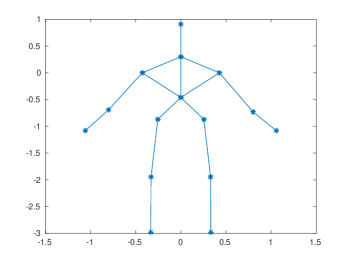
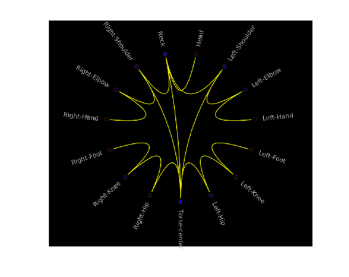
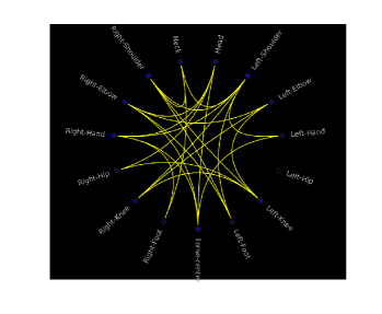
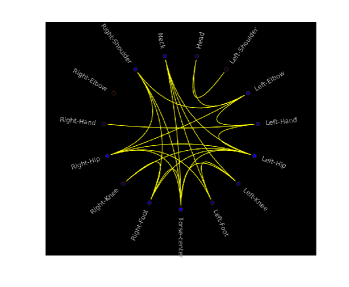
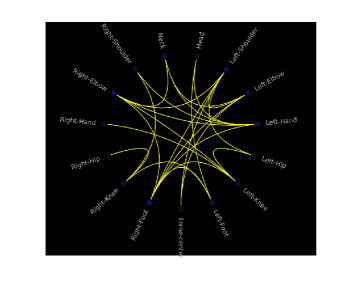
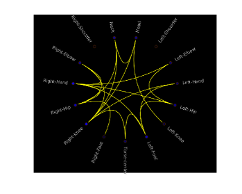
Figure 2: This figure shows (top) an original skeleton with its intrinsic node-to-node relationships useful for person identification, and (middle/bottom) four types of extrinsic node-to-node relationships found to be the most discriminating for action recognition when using the method introduced in this paper (the exact setting corresponds to Table I, with our learned matrix operators, using the orthogonality constraint and $K=4$). (Better to zoom the PDF version to view the learned node-to-node relationships).

6 Conclusion

We introduce in this paper a novel method which learns different matrix operators that ”optimally” define the support of aggregations and convolutions in graph convolutional networks. We investigate different settings which allow extracting non-differential and differential features as well as their combination before applying convolutions. We also consider different constraints (including orthogonality and stochasticity) which act as regularizers on the learned matrix operators and make their learning efficient while being highly effective. Experiments conducted on the challenging task of skeleton-based action recognition show the clear gain of the proposed method w.r.t different baselines as well as the related work.

References

- [1] D. Haussler. Convolution kernels on discrete structures. Technical report, Technical report, Department of Computer Science, University of California, 1999.
- [2] H. Sahbi. ”Kernel PCA for similarity invariant shape recognition.” Neurocomputing 70.16-18 (2007): 3034-3045.
- [3] X. Dong, D. Thanou, M. Rabbat, and P. Frossard, Learning graphs from data: A signal representation perspective, arXiv preprint arXiv:1806.00848, 2018.
- [4] S.I. Daitch, J.A. Kelner, and D.A. Spielman, Fitting a graph to vector data, in Proc. of ICML, 2009, pp. 201-208.
- [5] V. Kalofolias, How to learn a graph from smooth signals, in Proc. of the conf. on Artificial Intelligence and Statistics, 2016, pp. 920-929.
- [6] H.E. Egilmez, E. Pavez, and A. Ortega, Graph learning from data under structural and laplacian constraints, arXiv preprint arXiv:1611.05181,2016.
- [7] H. Sahbi, D. Geman, ”A Hierarchy of Support Vector Machines for Pattern Detection.” Journal of Machine Learning Research 7.10 (2006).
- [8] S.P. Chepuri, S. Liu, G. Leus, and A.O. Hero, Learning sparse graphs under smoothness prior, in Proc. of ICASSP, 2017, pp. 6508-6512.
- [9] B. Le Bars, P. Humbert, L. Oudre and A. s Kalogeratos. Learning Laplacian Matrix from Bandlimited Graph Signals. In ICASSP, 2019
- [10] H. Sahbi, J-Y. Audibert, and R. Keriven. ”Context-dependent kernels for object classification.” IEEE transactions on pattern analysis and machine intelligence 33.4 (2010): 699-708.
- [11] D. Valsesia, G. Fracastoro, and E. Magli, Sampling of graph signals via randomized local aggregations, arXiv preprint arXiv:1804.06182, 2018.
- [12] S. Sardellitti, S. Barbarossa, and P. Di Lorenzo, Graph topology inference based on transform learning, in Proc. of the Global Conf. on Signal and Information Processing, 2016, pp. 356-360.
- [13] Yuan, F., Xia, G. S., H. Sahbi, and Prinet, V. (2012). Mid-level features and spatio-temporal context for activity recognition. Pattern Recognition, 45(12), 4182-4191.
- [14] S. Sardellitti, S. Barbarossa, and P. Di Lorenzo. Graph topology inference based on sparsifying transform learning. IEEE TSP, 67(7), 2019.
- [15] X. Dong, D. Thanou, P. Frossard, and P. Vandergheynst, Learning Laplacian matrix in smooth graph signal representations, IEEE Trans. Signal Processing, vol. 64, no. 23, pp. 6160-6173, 2016.
- [16] B. Pasdeloup, V. Gripon, G. Mercier, D. Pastor, and M. G. Rabbat. Characterization and inference of graph diffusion processes from observations of stationary signals. IEEE TSIPN, 2017.
- [17] N. Bourdis, D. Marraud, and H. Sahbi. ”Camera pose estimation using visual servoing for aerial video change detection.” 2012 IEEE International Geoscience and Remote Sensing Symposium. IEEE, 2012.
- [18] D. Thanou, X. Dong, D. Kressner, and P. Frossard. Learning heat diffusion graphs. IEEE TSIPN, 3(3):484–499, 2017.
- [19] K. Yun, J. Honorio, D. Chattopadhyay, T-L. Berg, and D. Samaras. The HAU3D-CVPR Workshop, CVPR 2012.
- [20] J. Liu, A. Shahroudy, D. Xu, and G. Wang. Spatio-temporal LSTM with trust gates for 3D human action recognition. In ECCV, 2016
- [21] H. Sahbi and N. Boujemaa. ”Robust matching by dynamic space warping for accurate face recognition.” Proceedings 2001 International Conference on Image Processing (Cat. No. 01CH37205). Vol. 1. IEEE, 2001.
- [22] L. Shi, Y. Zhang, J. Cheng, and H. Lu. Two-stream adaptive graph convolutional networks for skeleton-based action recognition. CVPR, 2019
- [23] Y. Du and W. Wang and L. Wang. Hierarchical Recurrent Neural Network for Skeleton Based Action Recognition. CVPR, 2015
- [24] H. Sahbi and N. Boujemaa. ”Validity of fuzzy clustering using entropy regularization.” The 14th IEEE International Conference on Fuzzy Systems, 2005. FUZZ’05.. IEEE, 2005.
- [25] S. Yan and Y. Xiong and D. Lin. Spatial Temporal Graph Convolutional Networks for Skeleton-Based Action Recognition. AAAI, 2018
- [26] A. Kacem, M. Daoudi, B. Ben Amor, S. Berretti, J-Carlos. Alvarez-Paiva. A Novel Geometric Framework on Gram Matrix Trajectories for Human Behavior Understanding. IEEE TPAMI, 28 September 2018
- [27] E. Benhaim, H. Sahbi, and G. Vitte. ”Designing relevant features for visual speech recognition.” 2013 IEEE International Conference on Acoustics, Speech and Signal Processing. IEEE, 2013.
- [28] M. Maghoumi, JJ. LaViola Jr. DeepGRU: Deep Gesture Recognition Utility. In arXiv preprint arXiv:1810.12514, 2018
- [29] P. Vo, H. Sahbi,. Transductive kernel map learning and its application to image annotation. In: BMVC. pp. 1–12 (2012)
- [30] J. Liu, G. Wang, L. Duan, K. Abdiyeva, and A. C. Kot. Skeleton-based human action recognition with global context-aware attention lstm networks. IEEE TIP, 27(4):1586–1599, April 2018
- [31] Q. Oliveau and H. Sahbi. ”Learning attribute representations for remote sensing ship category classification.” IEEE Journal of Selected Topics in Applied Earth Observations and Remote Sensing 10.6 (2017): 2830-2840.
- [32] S. Song, C. Lan, J. Xing, W. Zeng, and J. Liu. An end-to end spatio-temporal attention model for human action recognition from skeleton data. In AAAI, 2017
- [33] P. Zhang, C. Lan, J. Xing, W. Zeng, J. Xue, and N. Zheng. View adaptive recurrent neural networks for high performance human action recognition from skeleton data. In ICCV, 2017
- [34] Y. Du, W. Wang, and L. Wang. Hierarchical recurrent neural network for skeleton based action recognition. In CVPR, 2015
- [35] W. Zhu, C. Lan, J. Xing, W. Zeng, Y. Li, L. Shen, and X. Xie. Co-occurrence feature learning for skeleton based action recognition using regularized deep LSTM networks. In AAAI, 2016
- [36] L. Wang and H. Sahbi. ”Nonlinear cross-view sample enrichment for action recognition.” European Conference on Computer Vision. Springer, Cham, 2014.
- [37] W. Li, L. Wen, M. Choo Chuah, and S. Lyu. Category-blind human action recognition: A practical recognition system. In ICCV, 2015
- [38] Y. Ji, G. Ye, and H. Cheng. Interactive body part contrast mining for human interaction recognition. In ICMEW, 2014
- [39] H. Sahbi. ”Coarse-to-fine deep kernel networks.” Proceedings of the IEEE International Conference on Computer Vision Workshops. 2017.
- [40] M. Defferrard, X. Bresson, P. Vandergheynst. Convolutional Neural Networks on graphs with Fast Localized Spectral Filtering. In NIPS, 2016
- [41] A. Dutta and H. Sahbi. ”High order stochastic graphlet embedding for graph-based pattern recognition.” arXiv preprint arXiv:1702.00156 (2017).
- [42] F. Wu, T. Zhang, A. Holanda de Souza Jr., C. Fifty, T. Yu, K-Q. Weinberger. Simplifying Graph Convolutional Networks. In arXiv:1902.07153, 2019
- [43] TN. Kipf, M. Welling. Semi-supervised classification with graph convolutional networks. In ICLR, 2017
- [44] M. Ferecatu and H. Sahbi. ”Multi-view object matching and tracking using canonical correlation analysis.” 2009 16th IEEE International Conference on Image Processing (ICIP). IEEE, 2009.
- [45] F-M. Bianchi, D. Grattarola, C. Alippi, L. Livi. Graph Neural Networks with Convolutional ARMA Filters. In arXiv:1901.01343, 2019
- [46] H. Sahbi. ”CNRS-TELECOM ParisTech at ImageCLEF 2013 Scalable Concept Image Annotation Task: Winning Annotations with Context Dependent SVMs.” CLEF (Working Notes). 2013.
- [47] F. Baradel, C. Wolf, J. Mille. Pose-conditioned Spatio-Temporal Attention for Human Action Recognition. In arXiv preprint, 2017
- [48] Y. LeCun, Y. Bengio, and G. Hinton. ”Deep learning.” nature 521.7553 (2015): 436-444.
- [49] A. Krizhevsky, I. Sutskever, and G. E. Hinton, “Imagenet classification with deep convolutional neural networks,” in NIPS, 2012, vol. 60, pp. 1097–1105.
- [50] C. Szegedy, W. Liu, Y. Jia, P. Sermanet, S. Reed, D. Anguelov, D. Erhan, V. Vanhoucke, and A. Rabinovich, “Going deeper with convolutions,” in CVPR, 2015, pp. 1–9.
- [51] H. Sahbi, Jean-Yves Audibert, and Renaud Keriven. ”Graph-cut transducers for relevance feedback in content based image retrieval.” 2007 IEEE 11th International Conference on Computer Vision. IEEE, 2007.
- [52] K. He, X. Zhang, S. Ren, and J. Sun, “Deep residual learning for image recognition,” in CVPR, 2016, pp. 770–778.
- [53] G. Huang, Z. Liu, L. v. d. Maaten, and K. Q. Weinberger, “Densely connected convolutional networks,” in CVPR, 2017, pp. 2261–2269.
- [54] M. Jiu and H. Sahbi. ”Semi supervised deep kernel design for image annotation.” 2015 IEEE International Conference on Acoustics, Speech and Signal Processing (ICASSP). IEEE, 2015.
- [55] He, Kaiming, et al. ”Mask r-cnn.” Proceedings of ICCV, 2017.
- [56] S. Thiemert, H. Sahbi, and M. Steinebach. ”Applying interest operators in semi-fragile video watermarking.” Security, Steganography, and Watermarking of Multimedia Contents VII. Vol. 5681. International Society for Optics and Photonics, 2005.
- [57] Girshick, Ross. ”Fast r-cnn.” Proceedings of the IEEE ICCV, 2015.
- [58] M. Javad, et al. ”Fast YOLO: A fast you only look once system for real-time embedded object detection in video.” arXiv:1709.05943 (2017).
- [59] W. Zaremba, I. Sutskever, and O. Vinyals. ”Recurrent neural network regularization.” arXiv preprint arXiv:1409.2329 (2014).
- [60] N. Boujemaa, F., Fleuret, V. Gouet, and H. Sahbi. (2004, January). Visual content extraction for automatic semantic annotation of video news. In the proceedings of the SPIE Conference, San Jose, CA (Vol. 6).
- [61] M. Schuster and K.K. Paliwal. ”Bidirectional recurrent neural networks.” IEEE TSP 45.11 (1997): 2673-2681.
- [62] M. Jiu and H. Sahbi. ”Deep kernel map networks for image annotation.” 2016 IEEE International Conference on Acoustics, Speech and Signal Processing (ICASSP). IEEE, 2016.
- [63] Zhang, Ziwei, Peng Cui, and Wenwu Zhu. ”Deep learning on graphs: A survey.” IEEE Transactions on Knowledge and Data Engineering (2020).
- [64] C. Szegedy et al. ”Inception-v4, inception-resnet and the impact of residual connections on learning.” In AAAI, 2017.
- [65] Iandola, Forrest, et al. ”Densenet: Implementing efficient convnet descriptor pyramids.” arXiv:1404.1869 (2014).
- [66] Iandola, Forrest N., et al. ”SqueezeNet: AlexNet-level accuracy with 50x fewer parameters and 0.5 MB model size.” arXiv:1602.07360 (2016).
- [67] M. Jiu and H. Sahbi. ”Laplacian deep kernel learning for image annotation.” 2016 IEEE International Conference on Acoustics, Speech and Signal Processing (ICASSP). IEEE, 2016.
- [68] G. Ishaan, et al. ”Improved training of wasserstein gans.” In NIPS, 2017.
- [69] O. Ronneberger, P. Fischer, and T. Brox. ”U-net: Convolutional networks for biomedical image segmentation.” International Conference on Medical image computing and computer-assisted intervention. Springer, 2015.
- [70] L-C. Chen et al. ”Deeplab: Semantic image segmentation with deep convolutional nets, atrous convolution, and fully connected crfs.” IEEE TPAMI 40.4 (2017): 834-848.
- [71] J. Long, E. Shelhamer and T. Darrell. ”Fully convolutional networks for semantic segmentation.” In IEEE CVPR, 2015.
- [72] M. Jiu and H. Sahbi. Deep representation design from deep kernel networks. Pattern Recognition 88 (2019): 447-457.
- [73] J. Donahue and L-A. Hendricks and M. Rohrbach and S. Venugopalan and S. Guadarrama and K. Saenko and T. Darrell. LT Recurrent Convolutional Networks for Visual Recognition and Description. TPAMI, 2017
- [74] M. Arjovsky, A. Shah, Y. Bengio. Unitary Evolution Recurrent Neural Networks. ICML, 2016
- [75] V. Dorobantu, P.A. Stromhaug, and J. Renteria. Dizzyrnn: Reparameterizing recurrent neural networks for norm-preserving backpropagation. CoRR, abs/1612.04035, 2016
- [76] H. Sahbi and N. Boujemaa. ”From coarse to fine skin and face detection.” Proceedings of the 8th ACM international conference on Multimedia. 2000.
- [77] Z. Mhammedi, A.D. Hellicar, A. Rahman, and J. Bailey. Efficient orthogonal parametrisation of recurrent neural networks using householder reflections. In ICML, 2017
- [78] E. Vorontsov, C. Trabelsi, S. Kadoury, and C. Pal. On orthogonality and learning recurrent networks with long term dependencies. In ICML, 2017
- [79] S. Wisdom, T. Powers, J. Hershey, J. Le Roux, and L. Atlas. Full-capacity unitary recurrent neural networks. In NIPS, pages 4880—4888. 2016
- [80] H. Sahbi. Deep Total Variation Support Vector Networks. Proceedings of the IEEE International Conference on Computer Vision Workshops. 2019.
- [81] J. Chen, T. Ma, C. Xiao. Fastgcn: fast learning with graph convolutional networks via importance sampling. arXiv preprint arXiv:1801.10247 (2018)
- [82] M. Henaff, J. Bruna, Y. LeCun. Deep convolutional networks on graphstructured data. arXiv preprint arXiv:1506.05163 (2015)
- [83] J. Bruna, W. Zaremba, A. Szlam, Y. LeCun. Spectral networks and locally connected networks on graphs. arXiv preprint arXiv:1312.6203 (2013)
- [84] M. Defferrard, X. Bresson, P. Vandergheynst. Convolutional neural networks on graphs with fast localized spectral filtering. In NIPS, 3844-3852 (2016)
- [85] W. Huang, T. Zhang, Y. Rong, J. Huang. Adaptive sampling towards fast graph representation learning. In NIPS. pp. 4558-4567 (2018)
- [86] T.N. Kipf, M. Welling. Semi-supervised classification with graph convolutional networks. arXiv preprint arXiv:1609.02907 (2016)
- [87] R. Levie, F. Monti, X. Bresson, M.M. Bronstein. Cayleynets: Graph convolutional neural networks with complex rational spectral filters. IEEE Transactions on Signal Processing 67(1), 97–109 (2018)
- [88] R. Li, S. Wang, F. Zhu, J. Huang. Adaptive graph convolutional neural networks. In AAAI, 2018.
- [89] Z. Chenyi and Q. Ma. Dual graph convolutional networks for graph-based semi-supervised classification. Proceedings of WWW, 2018.
- [90] Y. Li, C. Meng, C. Shahabi, Y. Liu. Structure-informed Graph Auto-encoder for Relational Inference and Simulation. ICML, 2019
- [91] T. Kipf, E. Fetaya, KC. Wang, M. Welling, R. Zemel. Neural Relational Inference for Interacting Systems. ICML, 2018
- [92] F. Alet, A-K. Jeewajee, M. Bauza, A. Rodriguez, T. Lozano-Perez, L.P. Kaelbling. Graph Element Networks: adaptive, structured computation and memory. ICML, 2018
- [93] L. Wang and H. Sahbi. ”Directed acyclic graph kernels for action recognition.” Proceedings of the IEEE International Conference on Computer Vision. 2013.
- [94] F. Alet, T. Lozano-Perez, and L.P. Kaelbling. Modular meta-learning. In the 2nd Conference on Robot Learning, pp. 856–868, 2018.
- [95] L. Franceschi and M. Niepert and M. Pontil and X. He. Learning Discrete Structures for Graph Neural Networks. ICML, 2019.
- [96] Y. Chen, L. Wu, M.J. Zaki. Deep Iterative and Adaptive Learning for Graph Neural Networks. In AAAI DLGMA Workshop, 2020.
- [97] A. Micheli. Neural network for graphs: A contextual constructive approach. IEEE TNN 20(3), 498?511 (2009)
- [98] H. Sahbi. ”A particular Gaussian mixture model for clustering and its application to image retrieval.” Soft Computing 12.7 (2008): 667-676.
- [99] M. Gori, G. Monfardini, F. Scarselli. A new model for learning in graph domains. In IEEE IJCNN, vol. 2, pp. 729–734, 2005.
- [100] F. Scarselli, M. Gori, A.C. Tsoi, M. Hagenbuchner, G. Monfardini. The graph neural network model. IEEE TNN 20(1), 61–80, 2008.
- [101] Z. Wu, S. Pan, F. Chen, G. Long, C. Zhang, P.S. Yu. A comprehensive survey on graph neural networks. arXiv:1901.00596 (2019).
- [102] H. Sahbi. ”Imageclef annotation with explicit context-aware kernel maps.” International Journal of Multimedia Information Retrieval (2015): 113-128.
- [103] W. Hamilton, Z. Ying, J. Leskovec. Inductive representation learning on large graphs. In NIPS. pp. 1024–1034 (2017)
- [104] J. Zhang, X. Shi, J. Xie, H. Ma, I. King, D.Y. Yeung. Gaan: Gated attention networks for learning on large and spatiotemporal graphs. arXiv:1803.07294 (2018)
- [105] F. Monti, D. Boscaini, J. Masci, E. Rodola, J. Svoboda, M.M. Bronstein. Geometric deep learning on graphs and manifolds using mixture model cnns. In CVPR, pp. 5115–5124 (2017)
- [106] M. Niepert, M. Ahmed, K. Kutzkov. Learning convolutional neural networks for graphs. In ICML, pp. 2014-2023 (2016)
- [107] J. Atwood, D. Towsley. Diffusion-convolutional neural networks. In NIPS, pp. 1993–2001 (2016)
- [108] H. Gao, Z. Wang, S. Ji. Large-scale learnable graph convolutional networks. In the 24th ACM SIGKDD International Conference on Knowledge Discovery & Data Mining. pp. 1416–1424. ACM (2018)
- [109] H. Sahbi and F. Fleuret. ”Scale-invariance of support vector machines based on the triangular kernel.” (2002).
- [110] L. Chen, L. Duan and D. Xu, ”Event Recognition in Videos by Learning From Heterogeneous Web Sources,” in IEEE CVPR, 2013, pp. 2666-2673
- [111] D. Xu, S-F. Chang. Visual Event Recognition in News Video using Kernel Methods with Multi-Level Temporal Alignment. CVPR 2007
- [112] L. Wang, Y. Xiong, Z. Wang, Y. Qiao, D. Lin, X. Tang, and L. Van Gool. Temporal segment networks: Towards good practices for deep action recognition. ECCV, 2016
- [113] H. Sahbi, L., Ballan, G., Serra and A. Del Bimbo. (2012). Context-dependent logo matching and recognition. IEEE Transactions on Image Processing, 22(3), 1018-1031.
- [114] D. Tran and L. Bourdev and R. Fergus and L. Torresani and M. Paluri. Learning Spatiotemporal Features With 3D Convolutional Networks. ICCV, 2015
- [115] S. Martin, Z. Marinka, Z. Blaz, U. Jernej, C. Tomaz. Orthogonal matrix factorization enables integrative analysis of multiple RNA binding proteins. Bioinformatics, Volume 32, Issue 10, 15 May 2016, Pages 1527–1535
- [116] S. Ye, J. Liang, R. Liu, X. Zhu. Symmetrical Graph Neural Network for Quantum Chemistry, with Dual R/K Space. arXiv:1912.07256, 2019
- [117] L. Wang and H. Sahbi. ”Bags-of-daglets for action recognition.” 2014 IEEE International Conference on Image Processing (ICIP). IEEE, 2014.
- [118] D. Slepian. Some comments on Fourier analysis, uncertainty and modeling. In Society for Industrial and Applied Mathematics (SIAM review), 1983
- [119] T. Wang, R. Liao, J. Ba, and S. Fidler. Nervenet: Learning structured policy with graph neural networks. ICLR, 2018
- [120] A. Loukas. What graph neural networks cannot learn: depth vs width. ICLR, 2020
- [121] A. Atamna, N. Sokolovska and J-C. Crivello. ”A Principled Approach to Analyze Expressiveness and Accuracy of Graph Neural Networks.” In ISIDA. Springer, 2020.
- [122] H. Sahbi and F. Fleuret. ”Kernel methods and scale invariance using the triangular kernel.” (2004).
- [123] N. Yasunori. A note on Riemannian optimization methods on the Stiefel and the Grassmann manifolds. In NOLTA, volume 1, pages 349–352, 2005.
- [124] L. Huang, X. Liu, B. Lang, A. W. Yu, Y. Wang, and B. Li. Orthogonal weight normalization: Solution to optimization over multiple dependent Stiefel manifolds in deep neural networks. In AAAI, 2017.
- [125] H. Sahbi,P. Etyngier, J-Y. Audibert and R. Keriven (2008, June). Manifold learning using robust graph laplacian for interactive image search. In 2008 IEEE Conference on Computer Vision and Pattern Recognition (pp. 1-8). IEEE.
- [126] A. Shukla, S. Bhagat, S. Uppal, S. Anand, P. Turaga. PrOSe: Product of Orthogonal Spheres Parameterization for Disentangled Representation Learning. In BMVC, 2019.
- [127] M. Belkin and P. Niyogi. Lapl eigenmaps for dimensionality reduction and data representation. Neural computation 15.6 (2003): 1373-1396.
- [128] S. Thiemert, H. Sahbi, and M. Steinebach. ”Using entropy for image and video authentication watermarks.” Security, Steganography, and Watermarking of Multimedia Contents VIII. Vol. 6072. International Society for Optics and Photonics, 2006.
- [129] S. Kumar et al. ”A unified framework for structured graph learning via spectral constraints.” JMLR 21.22 (2020): 1-60.
- [130] Khalil, Elias, et al. ”Learning combinatorial optimization algorithms over graphs.” In NIPS, 2017.
- [131] Prates, Marcelo, et al. ”Learning to solve NP-complete problems: A graph neural network for decision TSP.” In AAAI. Vol. 33. 2019.
- [132] H. Sahbi and Xi Li. ”Context-based support vector machines for interconnected image annotation.” Asian Conference on Computer Vision. Springer, Berlin, Heidelberg, 2010.
- [133] Y. Li, R. Yu, C. Shahabi, and Y. Liu, Diffusion convolutional recurrent neural network: Data-driven traffic forecasting. In Proc. of ICLR, 2018.
- [134] J.B. Kruskal. ”On the shortest spanning subtree of a graph and the traveling salesman problem”. Proc of the AMS, 7 (1): 48-50, 1956.
- [135] H. Sahbi, Coarse to fine support vector machines for hierarchical face detection, Ph.D. thesis, PhD thesis, Versailles University, 2003.
- [136] S. Tollari, P. Mulhem, M. Ferecatu, H. Glotin, M. Detyniecki, H. Sahbi, and Z-Q. Zhao. ”A comparative study of diversity methods for hybrid text and image retrieval approaches.” In Workshop of the Cross-Language Evaluation Forum for European Languages, pp. 585-592. Springer, Berlin, Heidelberg, 2008.