A novel kinetic mechanism for the onset of fast magnetic reconnection and plasmoid instabilities in collisionless plasmas

Abstract

Magnetic reconnection can explosively release magnetic energy when opposing magnetic fields merge and annihilate through a current sheet, driving plasma jets and accelerating non-thermal particle populations to high energy, in plasmas ranging from space and astrophysical to laboratory scales [1, 2, 3, 4]. Through laboratory experiments and spacecraft observations, significant experimental progress has been made in demonstrating how fast dissipation and reconnection occurs in narrow, kinetic-scale current sheets [4, 5, 6]. However, a challenge has been to demonstrate what triggers reconnection and how it proceeds rapidly and efficiently as part of a global system much larger than these kinetic scales. Here we show experimentally the full development of a process where the current sheet forms and then breaks up into multiple current-carrying structures at the ion kinetic scale. The results are consistent with tearing of the current sheet, however modified by collisionless kinetic ion effects, which leads to a larger growth rate and number of plasmoids than observed in previous experiments [7] or compared to predictions from standard tearing instability theory [8] and previous non-linear kinetic reconnection simulations [9, 10]. This effect will increase the role of plasmoid instabilities in many natural reconnection systems and should be considered in triggering rapid reconnection in a broad range of natural plasmas with collisionless, compressible flows, including at the Earth’s magnetosheath [11, 12] and magnetotail [13] and at the heliopause [14], in accretion disks [15], and in turbulent high-Mach-number collisionless shocks [3].

In weakly collisional plasmas, current sheets typically thin to kinetic scales comparable to the ion skin depth $d_{i}=(m_{i}/\mu_{0}n_{e}Z_{{e\!f\!\!f}}e^{2})^{1/2}$ [2, 4, 5, 6]. In most astrophysical and space plasmas of interest, however, there is a very large separation of scales between global scales driving reconnection and the kinetic scales where dissipation occurs, which presents a challenge for understanding efficient conversion of magnetic field energy. The large scale separation from the global scale to kinetic and resistive scales is indicated by large values of the dimensionless system size $L/d_{i}$ and the Lundquist number $S=\mu_{0}LV_{A}/\eta$, where $L$ is the current sheet length, $V_{A}=B/\sqrt{\mu_{0}n_{i}m_{i}}$ is the Alfvén speed, and $\eta$ the plasma resistivity [16]. Theory and recent simulation have proposed how plasmoid instabilities [8, 9, 16, 17, 18, 19] grow and interact to generate turbulent flows near reconnection layers. The resulting plasmoid turbulence simultaneously forces a large number of narrow current sheets for fast dissipation while maintaining broad outflow layers for efficient global energy conversion. This scenario remains to be demonstrated in experiments, though the initial steps of this process are indicated by laboratory observations of individual plasmoids [7, 20, 21, 22, 23], or in spacecraft data which appears to cross such structures [13]. Experiments with high-energy laser-produced plasmas allow access to reconnection in such a large-system size regime, with current sheets much longer than both ion and electron kinetic scales, $L/d_{i}\sim 50$, and at large Lundquist number ($S\sim 1000$) [24] which can therefore address these questions [25]. We note this normalized system size approaches that for the Earth’s magnetotail (where $L\sim 10R_{E}\sim 100d_{i}$, where $R_{E}$ is the Earth’s radius). Using this technique, in this Letter we present laboratory experiments with collisionless ions in large-system size regime showing the formation and subsequent breakup of a reconnection current sheet. The results are consistent with tearing instabilities, though we observe larger growth rates, and a larger number of structures than were produced in previous experiments [7], or predicted by classical tearing instability theory [8, 26, 27] and previous non-linear kinetic reconnection simulations [10].

Experiments at the OMEGA EP Laser Facility were used to collide and merge two magnetized plasma plumes and drive reconnection (Fig. 1). Following the techniques of previous laser-driven reconnection experiments [28, 24, 29], a pair of expanding, interacting plasma plumes are generated with two laser pulses irradiating a pair of thin CH foils. As the plumes expand, they each self-generate a strong toroidal magnetic field ($B=~{}$20-40 T) by the Biermann battery effect, and, as the two plasmas merge together, these fields interact and reconnect. In these experiments we introduce a gap between two adjacent foils to allow diagnostic access for high resolution proton radiography, optical refractometry, and Thomson scattering of the reconnection layer (Fig. 1a,b). The colliding ablated flows compress the anti-parallel fields, leading to a strongly-driven magnetic reconnection in a compressible regime relevant to high Mach number shocks and other compressible flows in heliophysics and astrophysics. The plasma density and temperature is measured by Thomson scattering and ranges from $n_{e}=$ 1–3 $\times~{}10^{25}$ m^-3, with $T_{e}=$ 400–600 eV and $T_{i}=$ 1600–2400 eV. The corresponding plasma $\beta_{e}=2\mu_{0}n_{e}T_{e}/B^{2}=$ 2–8 and dynamic $\beta_{\textrm{dyn}}=\mu_{0}n_{i}m_{i}V_{in}^{2}/B^{2}=~{}$ 2.5–10, assuming inflows $V_{in}\approx$ 250 km/s at the time of reconnection. The ion skin depth $d_{i}\approx$ 60–100 $\mu$m demonstrates the large separation of scales between kinetic scales and the global length of the current sheet, $L_{CS}\sim 4$ mm =  40–80 $d_{i}$. The high plasma temperature implies a long ion mean-free-path ($\lambda_{ii}>$ 0.5 mm, between the counterflowing plasmas) and a high Lundquist number $S\sim$ 2500–4500. (Methods of establishing plasma parameters are discussed in the Supplementary and presented in Table S1).

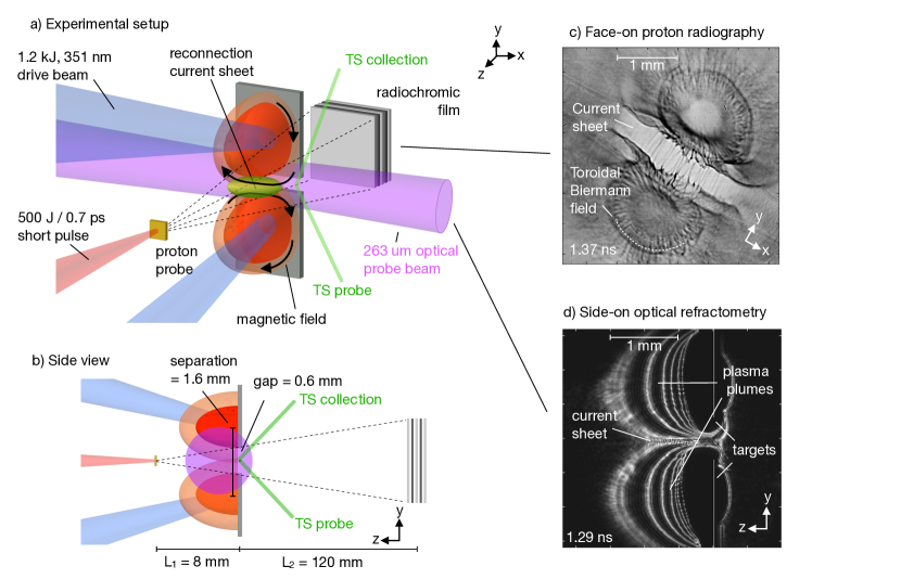
Figure 1: Experimental setup for observations of magnetic reconnection by proton radiography and optical refractometry. (a-b) The experiment consists of two parallel plastic (CH) foils, each driven by a 1.25 kJ, 1 ns laser at 351 nm to produce two expanding plasma plumes. We define a coordinate system where $x$ is in the plane of the foil and corresponds to the reconnection outflow direction, $y$ is in the plane of the foil corresponding to the reconnection inflow direction, and $z$ is perpendicular to the foil corresponding to the direction of plasma current flow in the current sheet. The two foils were separated by a gap of 600 $\mu$m. Thomson scattering is used to measure plasma density and separate electron and ion temperatures. The Thomson scattering volume was in the plane of the foils at a position $y=0.8$ mm “downstream” of the collision midpoint between the two plumes. (c) Proton radiography was obtained using a beam of fast protons produced by irradiating a Cu-foil with a short-pulse laser (480 J in 0.7 ps), which produced a high-time- ($\sim$ ps) and space-resolution ($<20~{}\mu$m) point source of protons with a broad energy distribution out to 10’s of MeV. The protons stream through the interaction region and deposit in a radiochromic film (RCF) stack, which provides energy resolution. The protons probed the plasma along the $z$-axis, yielding proton radiography images in the $x$-$y$ plane. An example film image is shown corresponding to 30 MeV protons. (d) Side-on optical probing was obtained with a 263 nm probe beam connected to an angular-filter refractometry (AFR) system. The beam propagated along the $x$-axis yielding images in the $y-z$ plane corresponding to density line-integrated in $x$. The bands map contours of constant gradient in line-averaged density, giving the global plume structure (Supplementary). The initial locations of the target foils are indicated by the gray lines.

Imaging data (Fig. 1c and d) shows the evolution of the magnetic fields and plasma density in the colliding plasmas. The proton radiography data (Fig. 1c) is obtained using a beam of high-energy protons, which streamed through the merging plasmas, and were recorded in a stack of radiochromic film. The protons experience small deflections from the transverse electric and magnetic fields along their trajectories, so that the fluence variations are related to the line-integrated electromagnetic fields [30]. For this geometry, protons respond to line-integrated magnetic field components ($\int B_{x}dz$ and $\int B_{y}dz$), which correspond to the reconnection inflow and outflow magnetic field components. Secondly, at these plasma parameters and proton-probing energies, the protons respond predominantly to magnetic rather than electric fields [31]. The radiographs are analyzed quantitatively below, but it is useful to first point out the qualitative features in the data. First, the thin dark circular feature, marked “Toroidal Biermann field”, is due to the proton focusing by the global toroidal field by the global Biermann battery effect in each plume. Where the plumes begin to merge and interact, a current sheet is formed, observed as a broad ($\sim 450$ $\mu$m) fluence depletion (light, marked “Current sheet”), bounded by two narrow fluence enhancements (dark), similar to observations in Ref. [24]. The fluence depletion is consistent with the defocusing of protons by the reversing magnetic field across the current sheet. Transverse fluence variations are also observed along the sheet, as well as around the plumes, related to small scale magnetic fluctuations. Side-on optical refractometry is simultaneously obtained using a 263 nm optical probe beam (Fig. 1d) to observe the plasma density. Significant plasma interaction is observed where the two plasmas meet and form the current sheet.

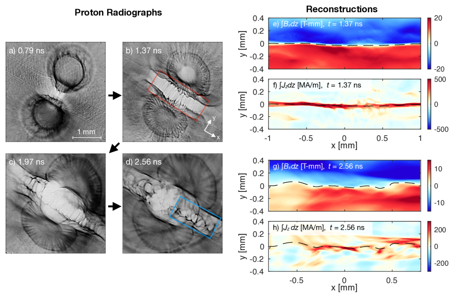
Figure 2: Proton radiography observations of current sheet formation and breakup. (a-d) Raw proton radiography data images at four times show the collision of two plumes. The images were obtained on separate shots, and therefore individual features cannot be tracked between frames, however the global features including the formation of an extended current sheet, and subsequent current-sheet breakup is apparent. The data correspond to film in the RCF stack corresponding to 30 MeV protons. (e,f) Reconstructions of the reconnecting magnetic field $(\int B_{x}dz$, panel e) and plasma current density ($\int J_{z}dz$, panel f) corresponding to the magenta box in the early-time (data 1.37 ns, panel b). (g,h) Same, corresponding to the blue box in the late time data (2.56 ns, panel d). The dashed line indicates the magnetic reversal surface, where $\int B_{x}dz=0$. The images (a-d) have been sharpened and contrast-adjusted, while data in (e-h) rely on processed raw data. The processing and reconstruction methodology is described in detail in the Supplementary.

A sequence of proton radiographs (Fig. 2) shows the full evolution of the interaction of the plumes, and formation and breakup of the current sheet. We present both the raw proton radiograph data (a-d), which contains valuable qualitative information, as well as quantitative reconstructions of the magnetic field $(\int B_{x}dz)$ and current ($\int J_{z}dz$) (e-h). Soon after the two plasmas meet (Fig. 2a, 0.79 ns), the current sheet region of reversing magnetic field forms, which quickly extends to nearly the full 3.5 mm field-of-view (by Fig. 2c, 1.97 ns). At early time, as the current sheet is forming, it is relatively uniform along its length (Fig. 2b, 1.37 ns) with relatively small current fluctuations evident in fine transverse proton modulations. However, by later time (Fig. 2c and d, 1.97 and 2.56 ns), the transverse modulations transition to a much higher-contrast with a cellular morphology. The amplitude of these structures is now very high, corresponding to $\sim$100% variations in the proton fluence.

A reconstruction of the plasma current sheet quantitatively demonstrates that these high-amplitude cellular structures correspond to a breakup of the current sheet. The reconstruction procedure [30] inverts the proton fluence maps to obtain the line-integrated magnetic fields and associated current density, where the line-integration is along the trajectory (primarily $\hat{z}$) of the probing protons. Figure 2e and f show the line-integrated magnetic field and plasma current density at the early time $t=1.37$ ns as the current sheet is forming. At this time, the current sheet is highly-extended and quasi-laminar, with half-width $a\equiv B_{up}/(dB/dy)=$30–40 $\mu$m. The upstream field $|\int B_{x}dz|$ is approximately 20 T-mm, and the peak line-integrated current density ($\int J_{z}dz$) is near 400 MA/m. Outside the current sheet, the current density is slightly negative, reflecting the closure of the current back through the plasma plumes.

The reconstruction at later time (2.56 ns, Fig. 2g and h) shows an evolution to a current sheet full of cellular structures. We focus reconstruction on a downstream region, centered approximately 0.8 mm from the midpoint and indicated by the blue box of Fig. 2d, as this is the region which shows significant current sheet dynamics. The $B_{x}=0$ surface, marked with a dashed line, has become highly kinked and folded. The upstream fields have also weakened somewhat to $|\int B_{up}dz|\sim$ 15 T-mm). Most importantly, the current density has become highly modulated, with near 100% modulations in the current density. The typical scale of the current modulation is 200 $\mu$m.

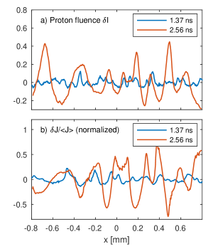
Figure 3: Profiles of proton fluence and current density along the current sheet. a) Proton fluence cuts along the center of the current sheet ($y=0$) at early (1.37 ns) and late (2.56 ns). b) Corresponding reconstructed current density ($\int J_{z}dz$) profiles following the current sheet structure, normalized to the average along the current sheet. Both have been filtered to remove the mean and long-scale variations ($\lambda>500$ um) to focus on the variations.

We examine profiles of the raw proton and reconstructed current density fluctuations in Fig. 3, corresponding to profiles taken along $B_{x}=0$. For each, we filter to isolate modulations with wavelength $<500$ $\mu$m, and for the current we normalize to the average current in the current sheet. Both the protons fluctuation ($\delta I$) and current density fluctuations ($\delta J/J$) increase significantly, with the RMS increasing by a factor of $\sim$4 between the two time points. The data show a strong relation between raw proton fluence and plasma current. This is important as this confirms the relation between high-contrast cellular proton fluence structures in the raw data (Fig. 2d) with the breakup of the current structures (Fig. 2h).

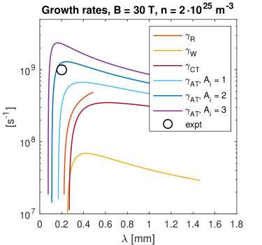
Figure S4: Instability growth calculations for various theories under experimental parameters for various wavelength. The theory models are described in the text. The experimentally-estimated growth rate to generate structures at $\lambda=200~{}\mu$m is indicated as the circular data point.

Given that the proton measurement is line-integrating, we examined whether the late-time data indicate that current sheet itself has been folded and broken up, or whether it can be explained by the superposition of a laminar current sheet with another independent, modulated magnetic field created by another process. The evidence that the current sheet itself has been strongly folded and broken up is that the late-time data no longer shows any amount of the relatively clean early-time (1.37 ns) current sheet. The key question is therefore to examine if current sheet instabilities can explain the breakup of the current sheet into multiple current carrying structures. Taking the current modulation scale as indicative of the instability, and peaking at wavelengths $\lambda=2\pi/k$ near 200 $\mu$m, we evaluate $ka\approx 1$, where the current sheet half-width $a=30-40~{}\mu$m is obtained from the early-time magnetic profiles. Based on the growth of magnetic fluctuations (Fig. 3, the instability growth rate $\gamma$ is in excess of $10^{9}$ s^-1, but we note is likely fully into the non-linear regimes at late times when the current sheet is nearly entirely broken up. A natural mechanism to drive the breakup is the tearing instability. However, the wavelength is smaller than expected for classical tearing, which is stabilized for $ka\gtrsim 1$. We evaluated classical (resistive) [32, 8] and collisionless [26] tearing for experimental parameters (Fig. S4), which both predict linear growth rates too slow to explain these dynamics as well as fastest-growing wavelengths longer than observed. For this reason, it is also perhaps not surprising that the typical wavelength is also significantly shorter than observed in recent nonlinear kinetic particle-in-cell simulations initiated from a Harris sheet [10] or under laser-plasma conditions [33].

We find the growth at shorter-wavelength may be explained by coupling of tearing to plasma temperature anisotropy, so-called anisotropic tearing, which was proposed previously as a mechanism to trigger reconnection in the magnetotail [34, 35, 36]. The anisotropy couples a mirror- (or Weibel-type) instability to the tearing dynamics and boosts growth rates and produces current-sheet-breakup at shorter wavelengths. Phase-space anisotropy of the ions can develop from counterstreaming ions or possibly compressive perpendicular heating resulting from the strong inflows, parameterized by $\alpha=T_{\perp,{e\!f\!\!f}}/T_{||}-1$, where $T_{\perp,eff}=M_{i}V_{in}^{2}+T_{\perp}$, and where the directions for $T_{\perp}$ and $T_{||}$ are with respect to the upstream field.

For the present experiments, using $t=2$ ns, we estimate an anisotropy up to $\alpha~{}\approx~{}$4 forms in C⁶⁺ populations due to the strong plasma inflow, $V_{in}\sim$ 250 km/s, compared to the measured $T_{||}~{}\sim~{}$2 keV. Figure S4 shows a calculation of growth rate versus wavelength for various tearing models, including anisotropic tearing for several values of anisotropy. Whereas classical (isotropic) tearing is stable at $\lambda=200~{}\mu$m, ion anisotropy boosts the growth rates and shifts the fastest-growing wavenumbers to $ka=~{}$1–2 [36], which can therefore explain the observations. (While challenging to estimate due to their collisionality, anisotropy developing in the electron populations can also strongly boost growth rates [36].) Interestingly, anisotropic tearing also has a much larger growth rate than a pure Weibel instability (at $B=0$, calculated in Fig. S4, also pointed out by Ref. [36]), owing to the presence of the current sheet which magnetizes the electrons which allows the mode to grow more rapidly. While pure ion-type Weibel instability was observed in previous laser experiments [37, 38], the present observations are at finite magnetic field and the morphology is apparently different, leading to closed cell magnetic structures rather than extended filaments.

The observations motivate particle-in-cell plasma simulations to probe the interaction between these instabilities and reconnection. We use the particle-in-cell simulation code PSC initialized with plasma flow, density, and temperature profiles obtained from a DRACO radiation-hydrodynamics simulation, benchmarked against the observed density evolution, and with magnetic fields consistent with the observed fields (Fig. 2f, the setup and codes are discussed in the Supplementary). Figure 4 shows a full 3-D visualization from the simulation of the structures formed during reconnection in the current sheet. These large-scale simulations keep the full system size in the inflow direction ($L/d_{i0}\approx 100$). In systems of this size, during the compression phase, current sheet is broken into a large number of plasmoids. Synthetic proton radiography is obtained by ray-tracing protons from a point-source, through the simulation volume, and then projecting them ballistically to a detector plane, where a fluence map is obtained. The pattern obtained shows the “cellular” structures which wrap around the O-points formed by reconnection, showing how the change in magnetic topology and reconnection is manifested in the radiography.

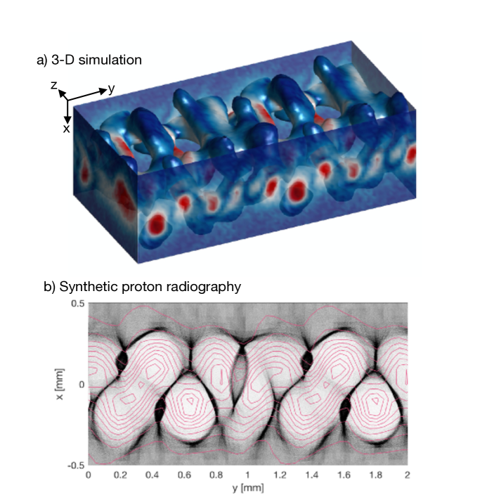
Figure 4: Simulations of colliding plasmas under experimental conditions. a) The 3-D visualization plasma current density (color) plotted atop iso-contours of plasma density. The face surfaces display current density, showing the formation of a large number of magnetic islands (high current density in red). b) Synthetic proton radiography obtained from line-integrating (along $z$) through the simulation fields, showing the development of multiple cellular plasmoid structures from the reconnection of magnetic fields. Following the conventions of the experimental film, higher proton fluence is rendered as darker. The magenta lines follow directly the simulation line-integrated magnetic fields $\int\mathbf{B}_{x,y}dz$, and are included to show the connection between cellular structures in the proton radiography and change in the averaged magnetic topology. Because of the 1-D nature of the plasma inflow initial condition used in the PIC simulation, a larger plasma compression is observed than in recent full 3-D simulations of similar systems, where the extra dimensionality allows a transverse dilation of the plasma. To account for this, we rescale the simulation length scales by matching the local ion-skin depth to the experiment.

These results show the full development of the formation and breakup of a current sheet at a large-system size, high-Lundquist number and collisionless-ion regime. The fast growth of instabilities at short wavelength ($ka\approx 1$) indicates the likely role of anisotropic tearing driven by collisionless ions. These instabilities will boost reconnection rates and increase the number of plasmoids generated compared to pure tearing instability theory, which has implications for observational signatures and more broadly for enhancing reconnection in a number of space plasma and astrophysical systems, for example driving “seas of plasmoids” in the heliosheath [14, 39], and driving electron-scale turbulent reconnection in the Earth magnetosphere [12]. These results demonstrate a rich physics connecting the evolution of magnetic fields to the formation of non-thermal plasma distributions and to kinetic instabilities, important to energy conversion and transport processes in collisionless astrophysical and space plasmas, which can now be studied in the laboratory, and may be observed in space plasmas with rapid phase space measurements made possible by the Magnetosphere Multiscale Mission [4].

1 Acknowledgments

The authors thank the OMEGA EP team for carrying out the experiments. Experiment time was made possible by grant DE-NA0003613 provided by the National Laser User Facility. Simulations were conducted on the Titan supercomputer at the Oak Ridge Leadership Computing Facility at the Oak Ridge National Laboratory through the Innovative and Novel Computational Impact on Theory and Experiment (INCITE) program, which is supported by the Office of Science of the DOE under Contract DE-AC05-00OR22725. This research was also supported by the DOE under Contracts DE-SC0008655, DE-SC0008409, and DE-SC0016249, and DE-AC02-09CH11466.

Appendix S Supplementary Materials

S.1 Detailed experimental setup

Experiments were conducted at the OMEGA EP facility at the University of Rochester Laboratory for Laser Energetics. Two 6 mm $\times$ 4 mm plastic (CH) targets of thickness 25 $\mu$m were aligned in a common plane, separated by a uniform gap of 600 $\mu$m (Fig. 1a and b). The two main plasma plumes were each driven by a 1.25 kJ, 1 ns pulse of 351 nm ($3\omega$) light, with foci separated across the gap by 1600 $\mu$m. Phase plates were used which produced two smoothed beam profiles with $1/e$ radius of 340 um and with a supergaussian intensity profile with index 8. The peak intensity was near 3$\,\times\,10^{14}$ W/cm². Over all shots analyzed from OMEGA EP in this study, the mean laser-energy-per plume was 1.25 kJ, with the full range from 1.21 to 1.29 kJ, for a laser reproducibility of $\pm 3\%$.

A fast beam of probing protons was produced by a third, short-pulse IR ($1\omega$) laser, 480 J in 0.7 ps, focused to a spot size of $<25~{}\mu$m on a thin Cu foil. The thin Cu target was mounted in a backlighter assembly which is shielded from the expanding plasma with an additional thin Ta foil, all mounted in a 1 mm-diameter CH cylinder. The short pulse produced a population of high energy probing protons with a broad distribution of energies out to $>$ 40 MeV by the target-normal sheath acceleration mechanism [40]. Over several shots, the probing protons were variably timed with respect to the main drive plumes to radiograph different points of the plasma evolution and collision.

The probe protons pass through the plasmas of interest, and pick up deflections to their trajectories by electric and magnetic field structures in the plasmas, after which they propagate ballistically to a radiochromic film (RCF) stack. The stack of film provides energy resolution due to the varying Bragg peak with proton energy. For these experiments the proton source was $L_{1}$ = 8 mm from the foil plane, and detector $L_{2}$ = 120 mm from the foil plane, for a geometrical magnification of $M=16$. Distances in Figs. 1 and 2 are given in units in the plasma plane. A full discussion of the processing and analysis of the proton probing data is given in section S.5.

In addition to proton probing, additional plasma measurements were obtained using angular-filter refractometry of an optical probe beam, discussed in Section S.2. In addition, surrogate experiments were fielded at OMEGA which allowed a Thomson-scattering measureent of plasma density ($n_{e}$) and electron and ion temperatures ($T_{e},T_{i}$), discussed in section S.3.

S.2 Angular refractometry density measurement

A 263 nm ($4\omega$) optical probe beam was used to probe the plasma density evolution from the side-on, providing imaging data on the evolution of the plasma density. Optical probing provides data related to plasma density line-integrated along the beam path; in this experimental setup, the 4$\omega$ beam propagates along the $y$-axis, which is along the current sheet. The $4\omega$ probe beam was configured with both angular-filter refractometry (AFR) and shadowgraphy legs.

This section describes the AFR data processing and plasma density results. For AFR, a mask placed at the Fourier plane produces bright and dark bands in the final image, which map the contours of the refractive index of the plasma [41]. This information both displays the qualitative evolution of the plumes and can be quantitatively processed [42]. AFR [41] uses a “bulls-eye” mask placed at the optical Fourier plane, which masks certain refractive angles. Transitions from light-to-dark and vice-versa correspond to fixed values of the plasma refraction angle $|\mathbf{\theta}|$, where

$$\mathbf{\theta}=\frac{1}{2n_{e,cr,4\omega}}\mathbf{\nabla}_{\perp}\int n_{e}d\ell.$$ (1)

Qualitatively, the bands correspond to contours of constant $|\nabla n|$.

Both single and colliding plasmas were probed over a series of shots. We describe two analyses. First, a 1-D analysis is readily accomplished along the vertical axis of each plume. This can be processed to directly obtain the line-integrated density as a function of height ($z$), and this data is a useful support of the reproducibility of the plasmas from shot to shot. Second, for single plumes, the entire plume can be analyzed using a reconstruction procedure and assuming azimuthal symmetry, which provides a full density map.

The 1-D analysis provides valuable baseline plasma evolution information for comparison against simulations and confirming the high reproducibility between shots. Along the central (vertical) expansion axis of each plume, the density profile is nearly 1-D ($\partial/\partial z\gg\partial/\partial x=0$), and we therefore analyze Eq. 1 as a 1-D equation in $z$ along the expansion axis. We locate the AFR transitions in the image, which provide a locus of points $\{z_{j}\}$, for the $j$th AFR transition, and where the transition refraction angles $\{\theta_{j}\}$ are known based on the AFR filter construction and calibration [41]. In between these points, the refraction angle is interpolated in log-space, which is the the logical choice for a quasi-exponential profile, producing $\theta(z)$. Finally, the line-integrated density is obtained by integrating Eq. 1. Figure S1 shows the line-integrated densities along the plume axis for several shots clustered at times ($t=$ 1.3, 2.5 ns) corresponding to the times analyzed in Fig. 2. The plasma profiles are well-reproduced at each time indicating the high-reproducibility of the laser performance and plasma production.

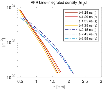
Figure S1: AFR Line-integrated density observations for early ($t=1.25$ ns), and late time ($t=2.5$ ns), corresponding to the two time points analyzed extensively in the proton radiography data. The observation time was repeated over several shots, both with double-plumes and with single plumes. The timing of the 4$\omega$ probe was directly measured for each shot and is indicated in the legend, as well as whether the shot was a single plume (’s’) or was the left (’l’) or right (’r’) plume of a double-plume shot.

Secondly, for single-plume shots, a reconstruction method is used to convert the line-integrated observations to density, assuming azimuthal symmetry [42]. Single plasmas are the most appropriate for reconstruction as they are reasonably azimuthally symmetric. A typical AFR image and associated reconstruction are shown in Fig. S2. This data is also useful as a comparison against single-point Thomson scattering measurements below.

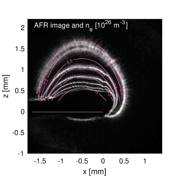
Figure S2: Angular filter refractometry image with overplotted reconstructed density for a single expanding plasma, $t=$ 1.35 ns. The target foil surface is denoted in gray.

S.3 Thomson scattering

Optical Thomson scattering (OTS) was used to provide direct measurements of plasma parameters during the plume interaction. OTS measurements were conducted on surrogate experiments at OMEGA, using identical targets and drive laser pointing. Each plume was driven by two overlapped OMEGA 3$\omega$ beams, with on-target laser energy of 950 J per plume, which is only slightly lower than the energies used at OMEGA EP. (Proton radiography was also obtained on these OMEGA shots, and qualitatively confirms the EP proton results presented in this paper, and which shows that the OMEGA shots were in a common regime.) A 527 nm ($2\omega$) Thomson scattering probe beam was passed through the plume interaction region. The scattering volume was directly in the gap between targets, in the plane of the foil, and at a distance $y=~{}0.8$ mm downstream from the direct midpoint between the plumes, which corresponds to the center of the blue inversion box of Fig. 2d. The scattered light was collected and split along two beam lines. One line passed through a lower resolution (150g/mm) spectrometer to collect spectra associated with electron plasma waves (EPW), while the other line passed through a high resolution (2160g/mm) spectrometer to collect spectra associated with ion acoustic waves (IAW). Each line was then detected on a separate streak camera with $\sim$50 ps temporal resolution.

The scattered power is proportional to the spectral density function

$$S(\mathbf{k},\omega)=\frac{2\pi}{k}\left|1-\frac{\chi_{e}}{\epsilon}\right|^{2}f_{e}\left(\frac{\omega}{k}\right)+\frac{2\pi Z}{k}\left|\frac{\chi_{e}}{\epsilon}\right|^{2}f_{i}\left(\frac{\omega}{k}\right)$$ (2)

where $\omega$ is the frequency, $\mathbf{k=k_{s}-k_{i}}$ is the wavevector being probed ($\mathbf{k_{i}}$ is the wavevector of the incident probe beam and $\mathbf{k_{s}}$ is the wavevector of the collected light), $Z$ is the ion charge state, $f_{e}$ and $f_{i}$ are the electron and ion distribution functions, respectively, $\chi_{e}$ and $\chi_{i}$ are the electron and ion susceptibilities, respectively, and $\epsilon=1+\chi_{e}+\chi_{i}$ is the longitudinal dielectric function [43]. The first term on the RHS of Eq. 2 corresponds to the EPW feature, while the second term corresponds to the IAW feature. Assuming Maxwellian distribution functions, plasma parameters can be extracted by iteratively fitting $S(\mathbf{k},\omega)$ to the measured spectra until a best fit is found. Error analysis is done using a Monte Carlo approach, in which the extracted plasma parameters represent the mean value over 50 fits, with the error bars corresponding to the standard deviation [44].

Four shots were analyzed. All data was collected from the same location, but two probe beam orientations were used (changing the scattering vector orientation compared to the foils). The results are shown in Fig. S3 for the electron temperature, electron density, and ion temperature. While the temperature values are consistent between orientations, the density is somewhat higher in one orientation. It is not clear if the difference is due to a relative pointing difference between shots (estimated to be small), or the presence of a density clump in the scattering volume in one of the shots (as the OTS measurement volume is smaller than the magnetic structures apparent in the proton radiography data). We take the density range as measure of the uncertainty and fold it into the analysis. We note that many key quantities such as the ion skin depth and Alfvén velocity depend relatively weakly on density ($\propto n_{e}^{-1/2}$), so errors in these quantities are relatively smaller.

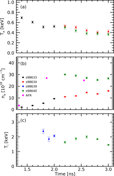
Figure S3: Thomson scattering measurements of the reconnection layer. a) Electron temperature. b) Electron density. c) Ion temperature. All values derived from analysis of the EPW and IAW spectra. Also shown in (b) are the electron densities measured with $2\times$ AFR (magenta squares).

The AFR density measurements were in good agreement with the Thomson scattering data. The Thomson scattering was obtained at a point in the target plane and a distance 0.8 mm in $x$ and 0.8 mm in $y$ compared to the center of the laser foci. To obtain a similar point from the AFR, we use single plume AFR data and evaluate at a point consistent with radius $r=0.11$ mm ($=0.8\times\sqrt{2}$) and in the foil plane. We multiple the AFR density by 2 to account for two plumes, which is in reasonable agreement and supports the TS data (Fig. S3).

S.4 Plasma parameters

Table S1 shows estimated plasma parameters in the current sheet in the region of the blue box of Fig. 2d, and at the time $t$=2 ns characteristic of the time when instabilities are growing and the current sheet is breaking up. The upstream magnetic fields and the current sheet width were determined from the analysis of magenta region in Fig. 2b at early time (t = 1.37 ns), where the current sheet is well-formed. To convert proton radiography observations (line-integrated magnetic fields), to an average magnetic field, we assumed a relation $\bar{B}=(1/L_{B})\int Bd\ell$ to obtain an average magnetic field, assuming an integration scale length $L_{B}$. We assume a broad range of possible $L_{B}$ of 0.5–1 mm, based by the plasma size as observed in side-on images (Fig. 1). The uncertainty in $L_{B}$ dominates the uncertainty in $\bar{B}$, and we fold this into uncertainties in parameters (such as $\beta$ and $S$) and theory comparisons below.

Plasma density and temperatures are obtained from Thomson scattering measurements, and we indicate the full range of values observed between 2.0 and 2.5 ns. The full range of values are folded in as uncertainties when estimating parameters (such as $S$ and $d_{i})$ and when comparing to theory. Inflow speeds are estimate based on a ballistic “time-of-flight” from the plasma birth location, near the edge of the laser focus at $r=350~{}\mu$m relative to each plume center, to the measurement location.

Table S1: Plasma parameters in reconnection current sheet, blue box of Fig. 2d

Density $n_{e}$ (m-3)	1–3$\,\times\,10^{25}$
Temperature $T_{e}$ (eV)	400–600
Temperature $T_{i}$ (eV)	1600–2400
Inflow speed $V_{in}$ (km/s)	250
Magnetic field $B$ (T)	20–40
Current sheet full-length $L_{cs}$ (mm)	4
Current sheet half-width $a=B_{up}/(dB/dx)$ ($\mu$m)	30–40
Instability wavelength $\lambda$ ($\mu$m)	200
Normalized wavenumber $ka$	0.9–1.1
$d_{i}$ (50–50 CH mixture) ($\mu$m)	60–100
$d_{e}$ ($\mu$m)	1–1.6
ion-ion MFP (C6+–C6+, between inflow populations) (mm)	0.5
Global Lundquist number $S=\mu_{0}LV_{A}/\eta$	2500-4500
Current sheet Lundquist number $S_{a}=\mu_{0}aV_{A}/\eta$	20–40
System size $L/d_{i}$	50
$\nu_{ei}/\omega_{ce}$	0.04 – 0.12
$\beta_{e}=2\mu_{0}n_{e}T_{e}/B^{2}$	2–8
$\beta_{\mathrm{dyn}}=\mu_{0}n_{i}m_{i}V_{in}^{2}/B^{2}$	2.5–10
electron magnetization $\omega_{ce}/\nu_{ei}$	15–50

S.5 Proton radiography analysis

Proton radiographs were obtained on HD-V2 film. For the qualitative radiography images presented (Fig. 2a-d), the data was sharpened using an unsharp-mask routine. Therefore the images are interpretive and do not quantitatively correspond to a physical proton dose. However, for all physics analysis (Fig. 2e-h), we start with the clean raw data, and apply a detailed processing and analysis chain which is now described.

In order to quantitatively analyze the radiographs, we use recent results [45] on the relation between proton dose and the film exposure, which shows the relation of the proton fluence (dose) to the film optical depth (OD), obtained from $OD_{\{RGB\}}=-log_{10}(T_{\{RGB\}})$ where $T_{\{RGB\}}$ is the transmission in red, green, or blue channels reported by the Epson scanner. The zero-exposure optical depth, $OD_{0}$, was obtained from unexposed RCF. The resulting background was subtracted from the $OD$s to produce a signal proportional to proton fluence. The linearity of $OD$ with dose has been studied [45] and is valid for the range of $OD$ we obtain. We found that applying a small color correction, $OD_{R*}=OD_{R}-\alpha_{R}OD_{B}$ and $OD_{G*}=OD_{G}-\alpha_{G}OD_{B}$, where $\alpha\sim 0.15-0.2$ improved the background subtraction and corrected some long-scale modulations in the film. (The $B$ channel itself has very low response to the proton dose, therefore mainly corrects any OD structuring the film substrate). To test the consistency and robustness of the results, we analyzed both $R*$ and $G*$ channels, as well as analyzed a several layers near the relevant energy, discussed below.

Proton radiographs are analyzed using a recent reconstruction algorithm [30]. The algorithm solves for the deflection magnetic field ($\int B_{x}dz,\int B_{y}dz$) consistent with the observed proton fluence pattern. Previous proton-deflection experiments in this plasma parameter regime [31] showed that the magnetic field is the dominant effect (over electric fields) in deflecting protons, and therefore we regard proton deflections as strictly due to magnetic fields. The algorithm assumes zero-normal-deflection boundary conditions ($\int\mathbf{B}dz\times\mathbf{n}=0$, where $\mathbf{n}$ is the normal vector through the boundary). Therefore we chose reconstruction volumes which extend to $y=\pm 800$ $\mu$m, that is, to the offset of each laser focus. (This reconstruction volume is larger than the data presented in Fig. 2 which has been cropped to focus on the current sheet.) Based on the structure of the Biermann fields (azimuthal around each laser focus, though of course this is modified where the plumes interact), $B_{x}$ is expected to be small at these $y$ positions.

The reconstruction algorithm assumes that the “undisturbed” proton fluence before reaching the plasma is uniform. However, we found that minor changes to the proton fluence, especially at long-wavelength scales, can significantly modify the magnetic field pattern. This results fundamentally because proton fluence radiographs are most closely related to $B$-field gradients, i.e. plasma current density [46], and inferring magnetic fields from this requires a spatial integration which is sensitive to “DC” or long-wavelength offsets. Furthermore it is clear from examining radiographs in cases with $B=0$ that the proton beams are not perfectly uniform. However, the goal in this study is primarily to understand qualitative structures in the plasma current density, and our main analysis focuses on this quantity. To overcome proton fluence non-uniformity we devised a high-pass filter which damps long-scale non-uniformities in the proton signal. The results in Fig. 2 use a filter characterized by $FWHM=600$ $\mu$m.

To provide an uncertainty and robustness analysis of this procedure, we conducted various robustness and consistency checks. That is, we conducted an identical analysis using the neighboring layers in the film stack, and also compared both the $R*$ and $G*$ channels. The scan of the neighboring layers only made a moderate difference in the energy analyzed (24.7, 29.2, or 33.2 MeV, i.e. only $\pm~{}7\%$ in proton velocity), but had a larger difference (factor of 2) in the average proton fluence. Therefore the comparison of different layers and color channels is a useful test for uncertainty related to any film saturation effect, background subtraction, or any energy-dependent proton-beam aberrations. Second, we also tested different spatial filters applied to the data, from FWHM 400 $\mu$m to 800 $\mu$m. All these tests produced basically indistinguishable results, confirming that the results are not an artifact of the analysis procedure. As an example metric, the RMS $\delta J/J$, discussed in relation to Fig. 3, varied only $[-10\%,+20\%]$ over all these tests, versus the factor $\sim$4 change in this quantity from early to late time. These confirm the robustness of the results.

S.6 Tearing Instability Models

The tearing theory was generalized to anisotropic distribution functions for electrons and ions in several prior theoretical works [34, 35, 36]. Anisotropic tearing has attracted significant theoretical interest over the years as it is found to significantly increase the instability of current sheets and may thereby contribute to space physics phenomena such as magnetospheric substorm onset.

A fundamental parameter is the tearing instability index, the dimensionless quantity $a\Delta^{\prime}$, which is related to the free magnetic energy available to be released by current sheet breakup. (Often abbreviated $\Delta^{\prime}$, here we use $a\Delta^{\prime}$, where $a$ is a length scale related to the current-sheet profile, to be clear that we have a dimensionless quantity.). The tearing index depends on the current profile and instability wavelength. For the canonical current sheet profile with $B_{x}(y)\propto\tanh(y/a)$, and for transverse tearing perturbation $\xi\propto\exp(-ikx+\gamma t)$, it is given by,

$$a\Delta^{\prime}=2(1/ka-ka).$$ (3)

The quantity can change quantitatively for different current profiles, but generally changes sign to negative for $ka\gtrsim 1$, indicating a stabilization of the mode. This is a significant constraint for the present observations where $ka\approx 1$ is observed.

In the fluid regime, resistive dissipation leads to the classical resistive (Furth-Killeen-Rosenbluth) tearing [32, 8] with growth rate (in the constant-$\Psi$ regime),

$$\gamma_{R}=0.96\frac{V_{A}}{a}S_{a}^{-3/5}(a\Delta^{\prime})(ka)^{2/5}.$$ (4)

Here $S_{a}$ is the Lundquist number evaluated with the current sheet half-width, $S_{a}=\mu_{0}aV_{A}/\eta$.

The resistive tearing has been generalized to collisionless regimes [26] where electron Landau damping in the current sheet provides dissipation, and further generalized to the anisotropic tearing considering pressure anisotropy, where $T_{\perp}>T_{||}$ provides additional positive feedback driving instability growth [34, 35, 36]. For anisotropic tearing, we use the analytic formulas of Quest et al. [36] (Eq. (43), which were found to be in reasonable agreement with the full-orbit numerical calculations by the same authors. Here we use the analytic formulas because numerical calculations were not conducted in our parameter regime. In this theory, the growth rate of anisotropic ion tearing is given by,

$$\gamma_{AT}=kv_{te}\frac{\epsilon_{e}^{3/2}}{\beta_{e}}\left[\frac{\sqrt{\pi}}{2\cdot 2.96}(a\Delta^{\prime})+\frac{1}{\sqrt{\pi}}\sum_{j}\frac{\beta_{j}}{\epsilon_{j}^{3/2}}A_{j}\right].$$ (5)

Here the electron beta $\beta_{e}=2n_{e}T_{e}\mu_{0}/B^{2}$, and $\epsilon_{e}=\rho_{e}/a$. One recognizes the first term in brackets of Eq. 5 is the collisionless tearing drive ($\propto\Delta^{\prime}$), and the second related to anisotropic ions ($\propto A_{j}$). We generalized the treatment to sum over multiple ion species ($j$) which may have separate anisotropies $A_{j}=T_{\perp,{e\!f\!\!f},j}/T_{||,j}-1$, and with $\beta_{j}=2\mu_{0}n_{j}T_{\perp,{e\!f\!\!f},j}/B^{2}$, and $\epsilon_{j}=\rho_{j}/a$, where $\rho_{j}=m_{j}V_{\perp,j}/Z_{j}eB$. The equation was also simplified considering moderate ion anisotropy ($A_{j}\ll M_{i}/m_{e}$), and zero electron anisotropy ($A_{e}=0)$. Quest et al also introduce a modified expression for $a\Delta^{\prime}$, which we retained, however this term is really only important for very long wavelengths $ka\ll 1$. The pure collisionless tearing $\gamma_{CT}$ [26] is obtained from the $A_{j}=0$ limit of this equation. The anisotropic tearing can also be driven by electron anisotropy, and indeed can provide a stronger lever than ions and has therefore often been considered in space physics contexts [47, 36]. However since we infer rapid electron collisional isotropization in the present experiments, this effect is difficult to estimate, so we presently just consider the case $A_{e}=0$.

Interestingly, the anisotropic tearing obtains a larger growth rate than pure Weibel instability ($B=0$), for which the growth rate is given by [48],

$$\gamma_{W}=\frac{kv_{te}}{\sqrt{\pi}}\left[\sum_{j}\frac{(n_{j}/n_{e})Z_{j}^{2}}{M_{j}/m_{e}}A_{j}-k^{2}d_{e}^{2}\right],$$ (6)

Here $d_{e}$ is the electron skin depth. For this dispersion relation, we considered the ion-pinch dispersion relation of Davidson et al, in the limit $\gamma/kv_{te}<1$, and again moderate ion anisotropy. The difference between anisotropic tearing and pure Weibel is the presence of the current sheet, which magnetized the electrons, which increases the growth of the instability. This fact was pointed out by Quest et al [36].

We evaluate growth rate of these instabilities for experimental parameters versus $\lambda=2\pi/k$. We consider the typical parameters, $B_{up}=30$ T, $n_{e}=2\cdot 10^{25}$ m^-3, and a current sheet half-width $a$ = 35 $\mu$m. We consider drive by anisotropic C${}^{6}+$ ions, at a fraction 1/7 of the $n_{e}$ density, with variable anisotropy $A_{i}$ from 1–3 indicated in the legend. For experimental plasma inflows of order 250 km/s (based on time-of-flight) an anisotropy up to 4 is possible considering the measured $T_{i}=2000$ eV. We plot classical tearing (orange) for unstable $k$ from $S_{a}^{0.25}<ka<1$, which corresponds to unstable constant-$\Psi$ modes where the growth-rate of Eq. 4 applies. We also plot collisionless tearing (red), pure Weibel (Eq. 6) (yellow), and anistropic tearing with $A_{i}$ = 1–3, (blue through purple). It is found that classical modes and pure Weibel have too-low growth-rates and are stable at the observed structure size. Ion Anisotropy $>2$ is sufficient to drive the observed instability growth at $\lambda\approx 200~{}\mu$m and $\gamma>10^{9}$ s^-1. The small relative growth of the pure Weibel mode compared to anisotropic tearing is consistent with the calculations of Quest et al ([36], Fig. 8). Scanning parameters, we find similar curves and the conclusions do not change for $B_{up}=$20–40 T and density $n_{e}=$ 1–3 $\cdot 10^{25}$ m^-3.

S.7 Particle-in-cell simulation setup

The particle-in-cell code PSC [49] is used to simulate reconnection between colliding laser-plasmas following the general model which has been used previously [25, 33]. The rich dynamics include compression of opposing magnetic fields into an ion-scale current sheet with the simultaneously development of kinetic instabilities and plasmoid development. Here we focus on a simulation of current sheet formation and reconnection where strong ion anisotropy develops, to show how this instability can initiate the formation of a large number of plasmoids with quantitative similarity to the experimental observations.

The simulations are 3-D, but for computational reasons we simulate a relatively narrow slug from the global geometry. Accordingly, the simulations are initialized with two 1-D flows ($n=n(y),V_{y}=V_{y}(y),B_{x}=B_{x}(y)$, following the coordinate system of Fig. 1. The initial profiles are qualitatively similar to used previously [25, 50, 33], but modified for new DRACO [51] simulations of these gapped experiments. From these new simulations, the initial profiles are taken at a time after magnetic fields have been generated by the Biermann battery effect. Specifically, the profiles are obtained from a radial cut between the bubbles at a height $z=400~{}\mu$m. A reference density is obtained based on the peak plasma density from DRACO, $n_{0}=$1.25$\,\times\,10^{27}$ m^-3, which defines a global ion skin depth for normalizing the simulation box, $d_{i0}\approx 8~{}\mu$m, for a 50-50 CH mixture. (For simplicity the PSC simulation itself is conducted with a pure-ion plasma.) The two plume centers are separated by the global length scale $L_{x0}=200~{}d_{i0}$, making for a very large kinetic simulation, and we use dimensions $25\times 25~{}d_{i0}$ in the two transverse directions. The profile is a smooth gaussian core which transitions to a steeper exponential to agree with the DRACO profiles, and the initial density at the midpoint between the two plumes is $\sim 0.015~{}n_{0}$. The plumes are given a uniform initial temperature $T_{0}$. Oppositely polarized magnetic fields are initialized in each plume with magnitude $B_{0}=0.05(n_{0}T_{0})^{1/2}$. Two counter flows are initialized, again per DRACO, with profiles for each plume $V=V_{0}|x|/L_{x0}$, with $V_{0}/C_{s}=2$, where $C_{s}$ is the sound speed and $x$ the distance from the center of the plume. The initial condition was modified from previous simulations [25, 50, 33], to allow ion counterstreaming between the two plumes in the initial condition. As commonly used with explicit PIC simulations, we use a compressed ion-electron mass ratio $M_{i}/m_{e}=64$ as well as a compressed speed-of-light, characterized by $m_{e}c^{2}/T_{0}=25$.

We have found that due to the nature of the 1-D flows driving the simulation, the density and fields are strongly compressed compared to the experimental (AFR) measurements of the density. This is because the flows in the real system compress along the $x$-direction while simultaneously de-compressing along the $y$- and $z$-directions (vertical and down-current-sheet), whereas the simulation simply compresses in $x$. This and other 3-D effects were demonstrated in recent work [52] which simulated the full 3-D evolution and reconnection in these systems with two plumes expanding from a thin foil. However, those fully-3-D simulations were conducted at a smaller plume separation ($L_{sep}\sim 80d_{i,ab}$, where $d_{i,ab}$ is the ion skin depth evaluated at the ablation surface); unfortunately the present experimental system is too large ($L_{sep}\sim 400~{}d_{i,ab}$) to enable such a simulation with present capabilities. For this reason, we match simulations to experiments by (1) judicious initialization to match dimensionless parameters such as the plasma $\beta_{e}$ once the current sheet forms; and (2), when generating experimental observables such as proton radiography, re-scaling lengths to match the local ion-skin depth in the current sheet between simulation and experiment, and scaling the magnetic fields to the experimental values observed in the current sheet.

References

- [1] Masuda, S., Kosugi, T., Hara, H., Tsuneta, S. & Ogawara, Y. A loop-top hard X-ray source in a compact solar flare as evidence for magnetic reconnection. Nature 371, 495–497 (1994).
- [2] Yamada, M., Kulsrud, R. & Ji, H. Magnetic reconnection. Rev. Mod. Phys. 82, 603–664 (2010).
- [3] Matsumoto, Y., Amano, T., Kato, T. N. & Hoshino, M. Stochastic electron acceleration during spontaneous turbulent reconnection in a strong shock wave. Science 347, 974–978 (2015).
- [4] Burch, J. L. et al. Electron-scale measurements of magnetic reconnection in space. Science 352, aaf2939 (2016).
- [5] Ren, Y. et al. Experimental verification of the Hall effect during magnetic reconnection in a laboratory plasma. Phys. Rev. Lett. 95, 055003 (2005).
- [6] Fox, W. et al. Experimental Verification of the Role of Electron Pressure in Fast Magnetic Reconnection with a Guide Field. Phys. Rev. Lett. 118, 125002 (2017).
- [7] Hare, J. . D. et al. Anomalous Heating and Plasmoid Formation in a Driven Magnetic Reconnection Experiment. Phys. Rev. Lett. 118 (2017).
- [8] Bhattacharjee, A., Huang, Y. M., Yang, H. & Rogers, B. Fast reconnection in high-Lundquist-number plasmas due to the plasmoid Instability. Phys. Plasmas 16, 112102 (2009).
- [9] Daughton, W. et al. Role of electron physics in the development of turbulent magnetic reconnection in collisionless plasmas. Nat Phys 7, 539–542 (2011).
- [10] Daughton, W. et al. Transition from collisional to kinetic regimes in large-scale reconnection layers. Phys. Rev. Lett. 103, 065004 (2009).
- [11] Retinò, A. et al. In situ evidence of magnetic reconnection in turbulent plasma. Nature Phys. 3, 236–238 (2007).
- [12] Phan, T. D. et al. Electron magnetic reconnection without ion coupling in Earth’s turbulent magnetosheath. Nature 557, 202–206 (2018).
- [13] Chen, L. J. et al. Observation of energetic electrons within magnetic islands. Nature Phys. 4, 19–23 (2007).
- [14] Opher, M. et al. Is the Magnetic Field in the Heliosheath Laminar or a Turbulent Sea of Bubbles? Astrophys. J. 734, 71 (2011).
- [15] Hoshino, M. Angular Momentum Transport and Particle Acceleration During Magnetorotational Instability in a Kinetic Accretion Disk. Phys. Rev. Lett. 114 (2015).
- [16] Ji, H. & Daughton, W. Phase diagram for magnetic reconnection in heliophysical, astrophysical, and laboratory plasmas. Phys. Plasmas 18, 111207 (2011).
- [17] Shibata, K. & Tanuma, S. Plasmoid-induced-reconnection and fractal reconnection. Earth, Planets and Space 53, 473–482 (2001).
- [18] Loureiro, N. F., Schekochihin, A. A. & Cowley, S. C. Instability of current sheets and formation of plasmoid chains. Phys. Plasmas 14, 100703 (2007).
- [19] Uzdensky, D. A., Loureiro, N. F. & Schekochihin, A. A. Fast Magnetic Reconnection in the Plasmoid-Dominated Regime. Phys. Rev. Lett. 105, 235002 (2010).
- [20] Gekelman, W., Pfister, H. & Kan, J. R. Experimental Observations of Patchy Reconnections Associated with the Three-Dimensional Tearing Instability. J. Geophys. Res. 96, 3829–3833 (1991).
- [21] Fiksel, G. et al. Magnetic Reconnection between Colliding Magnetized Laser-Produced Plasma Plumes. Phys. Rev. Lett. 113, 105003 (2014).
- [22] Olson, J. et al. Experimental Demonstration of the Collisionless Plasmoid Instability below the Ion Kinetic Scale during Magnetic Reconnection. Phys. Rev. Lett. 116, 255001 (2016).
- [23] Jara-Almonte, J., Ji, H., Yamada, M., Yoo, J. & Fox, W. Laboratory Observation of Resistive Electron Tearing in a Two-Fluid Reconnecting Current Sheet. Phys. Rev. Lett. 117, 095001 (2016).
- [24] Rosenberg, M. J. et al. Slowing of Magnetic Reconnection Concurrent with Weakening Plasma Inflows and Increasing Collisionality in Strongly Driven Laser-Plasma Experiments. Phys. Rev. Lett. 114, 205004 (2015).
- [25] Fox, W., Bhattacharjee, A. & Germaschewski, K. Fast Magnetic Reconnection in Laser-Produced Plasma Bubbles. Phys. Rev. Lett. 106, 215003 (2011).
- [26] Coppi, B., Laval, G. & Pellat, R. Dynamics of the Geomagnetic Tail. Phys. Rev. Lett. 16, 1207–1210 (1966).
- [27] Baalrud, S. D., Bhattacharjee, A., Huang, Y. M. & Germaschewski, K. Hall magnetohydrodynamic reconnection in the plasmoid unstable regime. Phys. Plasmas 18, 092108 (2011).
- [28] Nilson, P. M. et al. Magnetic Reconnection and Plasma Dynamics in Two-Beam Laser-Solid Interactions. Phys. Rev. Lett. 97, 255001 (2006).
- [29] Fiksel, G. et al. Electron energization during merging of self-magnetized, high-beta, laser-produced plasmas. J. Plasma Phys. 87 (2021).
- [30] Bott, A. F. A. et al. Proton imaging of stochastic magnetic fields. J. Plasma Phys. 83 (2017).
- [31] Petrasso, R. D. et al. Lorentz Mapping of Magnetic Fields in Hot Dense Plasmas. Phys. Rev. Lett. 103, 085001 (2009).
- [32] Furth, H. P., Killeen, J. & Rosenbluth, M. N. Finite-Resistivity Instabilities of a Sheet Pinch. Phys. Fluids 6, 459–484 (1963).
- [33] Lezhnin, K. V. et al. Regimes of magnetic reconnection in colliding laser-produced magnetized plasma bubbles. Phys. Plasmas 25, 093105 (2018).
- [34] Chen, J. & Palmadesso, P. Tearing instability in an anisotropic neutral sheet. Phys. Fluids 27, 1198 (1984).
- [35] Burkhart, G. R. & Chen, J. Linear, collisionless, bi-maxwellian neutral-sheet tearing instability. Phys. Rev. Lett. 63, 159–162 (1989).
- [36] Quest, K. B., Karimabadi, H. & Daughton, W. Linear theory of anisotropy driven modes in a Harris neutral sheet. Phys. Plasmas 17, 022107 (2010).
- [37] Fox, W. et al. Filamentation Instability of Counterstreaming Laser-Driven Plasmas. Phys. Rev. Lett. 111, 225002 (2013).
- [38] Huntington, C. M. et al. Observation of magnetic field generation via the Weibel instability in interpenetrating plasma flows. Nature Phys. 11, 173–176 (2015).
- [39] Drake, J. F., Opher, M., Swisdak, M. & Chamoun, J. N. A Magnetic Reconnection Mechanism for the Generation of Anomalous Cosmic Rays. Astrophys. J. 709, 963 (2010).
- [40] Snavely, R. A. et al. Intense High-Energy Proton Beams from Petawatt-Laser Irradiation of Solids. Phys. Rev. Lett. 85, 2945–2948 (2000).
- [41] Haberberger, D. et al. Measurements of electron density profiles using an angular filter refractometera). Phys. Plasmas 21, 056304 (2014).
- [42] Angland, P., Haberberger, D., Ivancic, S. T. & Froula, D. H. Angular filter refractometry analysis using simulated annealing. Rev. Sci. Inst. 88, 103510 (2017).
- [43] Sheffield, J., Froula, D. H., Glenzer, S. H. & Luhmann, N. Plasma Scattering of Electromagnetic Radiation (Academic Press, 2011), 2nd edn.
- [44] Follett, R. K. et al. Plasma characterization using ultraviolet thomson scattering from ion-acoustic and electron plasma waves (invited). Rev. Sci. Inst. 87, 11E401 (2016).
- [45] Chen, S. N. et al. Absolute dosimetric characterization of Gafchromic EBT3 and HDv2 films using commercial flat-bed scanners and evaluation of the scanner response function variability. Rev. Sci. Inst. 87, 073301 (2016).
- [46] Graziani, C., Tzeferacos, P., Lamb, D. Q. & Li, C. Inferring morphology and strength of magnetic fields from proton radiographs. Rev. Sci. Inst. 88, 123507 (2017).
- [47] Karimabadi, H. Role of electron temperature anisotropy in the onset of magnetic reconnection. Geophys. Res. Lett. 31, L18801 (2004).
- [48] Davidson, R. C., Hammer, D. A., Haber, I. & Wagner, C. E. Nonlinear Development of Electromagnetic Instabilities in Anisotropic Plasmas. Phys. Fluids 15, 317–333 (1972).
- [49] Germaschewski, K. et al. The Plasma Simulation Code: A modern particle-in-cell code with patch-based load-balancing. J. Comp. Phys. 318, 305–326 (2016).
- [50] Fox, W., Bhattacharjee, A. & Germaschewski, K. Magnetic reconnection in high-energy-density laser-produced plasmas. Phys. Plasmas 19, 056309 (2012).
- [51] Radha, P. B. et al. Multidimensional analysis of direct-drive, plastic-shell implosions on OMEGA. Phys. Plasmas 12, 056307 (2005).
- [52] Matteucci, J. et al. Biermann-battery-mediated magnetic reconnection in 3d colliding plasmas. Phys. Rev. Lett. 121, 095001 (2018).