Rotating neutron stars without light cylinders

Abstract

We find a class of twisted and differentially rotating neutron star  magnetospheres that do not have a light cylinder, generate no wind and thus do not spin-down. The magnetosphere is composed of embedded differentially rotating flux surfaces, with the angular velocity decreasing as $\Omega\propto 1/r$ (equivalently, becoming smaller at the foot-points closer to the axis of rotation). For each given North-South self-similar twist profile there is a set of self-similar angular velocity profiles (limited from above) with a “smooth”, dipolar-like magnetic field structure extending to infinity. For spin parameters larger than some critical value, the light cylinder appears, magnetosphere opens up, and the wind is generated.

1 Introduction

Magnetospheres of pulsars are highly magnetized and relativistically rotating (Goldreich & Julian, 1969). Though the initial set-up is very simple - rotating magnetized sphere with dipolar magnetic field - the nonlinear effects of charges and currents on the open field lines modify the field and make the problem highly non-linear (Beskin et al., 1988; Contopoulos et al., 1999; Gruzinov, 2005; Spitkovsky, 2006).

Another complication comes from possible non-dipolar, current-carrying magnetospheric fields in the closed zone (Thompson et al., 2002; Parfrey et al., 2013; Lyutikov, 2013). Current-loaded magnetospheres, e.g.  slightly twisted dipole (so that the northern foot-point is at different azimuthal angle $\phi$ than the southern foot-point) are not the same as vacuum multipoles (though they can be expanded as a sum of). Qualitatively, a given twist of a field line concentrates at the point of lowest guiding field. Hence at the furthest point (along closed field lines) in a (nearly) dipolar magnetosphere. This is especially important for magnetar phenomena (Thompson et al., 2002; Parfrey et al., 2013; Lyutikov, 2013).

Yet another complication comes from possible differential rotation of the foot points. This is induced by the electron Hall dynamics in the neutron star crust (Goldreich & Reisenegger, 1992; Wood et al., 2014; Gourgouliatos et al., 2015). In a “Solar flare” model of magnetar activity Lyutikov (2006, 2015) slow, plastic twisting of footprints leads to kink instabilities, generation of flares and Coronal Mass ejections.

Overall the system becomes very complicated/nonlinear. This puts special emphasis on possible (semi)-analytical solutions, that solve the complicated mathematics problem, and yet can be easily traced to the first principles. In this paper we discuss a class of (quasi)-analytical solutions of pulsar magnetospheres with a highly unusual properties: rotating and twisted pulsar magnetospheres  without light cylinders.

2 Self-similar rotating and twisted magnetospheres

The workhorse of analytical investigation of pulsar magnetospheres  is the relativistic generalization of the Grad-Shafranov equation (Grad, 1967; Shafranov, 1966; Scharlemann & Wagoner, 1973; Michel, 1973; Beskin, 2009) which expresses the force balance in an axially symmetric magnetosphere. The conditions of zero-divergence of the magnetic field, the ideal condition and axial symmetry allow the force balance to be expressed as a single scalar equation for the shape of the magnetic flux function $\Psi(r,\theta)$. There is a mathematical problem, though: the source terms (the poloidal current and in the case of differentially rotating magnetosphere the spin) enter as terms that are functions of the solution itself, not as independent quantities. This leads to mathematical complication: the equation to be solved and the solution need to be found self-consistently.

Few analytical roads remain. First, one can prescribe $I(\Psi)$ and solve for $\Psi$. For example linear relations $I=\alpha\Psi$ lead to simple, linear and hence highly useful analytical solutions, spheromaks in spherical geometry. Alternatively, Lynden-Bell & Boily (1994) suggested a self-similar approach, where the structure has a power-law scaling with the spherical radius. (They were adopted to cylindrical coordinates by Lyutikov, 2020b). Twisted configurations of Lynden-Bell & Boily (1994) are especially useful for astrophysical magnetars (Thompson et al., 2002).

In what follows we generalize the non-linear self-similar solutions of twisted magnetospheres  of Lynden-Bell & Boily (1994) to twisted and differentially rotating configurations.

2.1 Self-similar twisted and rotating magnetospheres

For a stationary axially symmetric configuration the Grad-Shafranov prescription involves field parametrization

$${\bf B}=(\nabla\Psi)\times(\nabla\phi)+I(\Psi)(\nabla\phi)\mbox{}$$

$${\bf E}=-\nabla\Phi(\Psi)\mbox{}$$

$$\Omega=-\Phi^{\prime}.$$ (1)

The force-free force balance

$${\bf E}{\rm\,div\,}{\bf E}+(\nabla\times{\bf B})\times{\bf B}=0$$ (2)

gives then the Grad-Shafranov equation (Grad, 1967; Shafranov, 1966; Scharlemann & Wagoner, 1973; Beskin, 2009)

$$(1-r^{2}\sin^{2}\theta\Omega^{2})\Delta\Psi-2\frac{\left(r\partial_{r}\Psi+\cot\theta\partial_{\theta}\Psi\right)}{r^{2}}+II^{\prime}-(\nabla\Psi)^{2}r^{2}\sin^{2}\theta\Omega\Omega^{\prime}=0,$$ (3)

(factors of $4\pi$ omitted). ($\Omega$ is not the rate of shearing of foot-points, it’s an angular velocity of rotation of a give flux surface.)

Let’s look for self-similar solutions to (3) in a form of

$$\Psi=r^{-p}F(\theta)\mbox{}$$

$$I\propto\Psi^{\alpha}\mbox{}$$

$$\Omega=C_{2}\Psi^{\beta}$$ (4)

By dimensional analysis

$$\alpha=1+1/p,\mbox{}$$

$$\beta=1/p$$ (5)

so that the radial scaling of all the components of the magnetic field is $\propto r^{-2-p}$: The electric part has the same power-law scaling as the magnetic. (We also comment that for $p=0$ one recovers Michel’s solution $\Psi=1-\cos\theta$, but with arbitrary $\Omega(\theta)$, $I=(1/2)\sin^{2}\theta\Omega(\theta)$ Lyutikov, 2011).

The angular part of the Grad-Shafranov equation (3) then obeys

$$\left(p(1+p)F+C_{1}F^{1+2/p}+(1-\mu^{2})F^{\prime\prime}\right)-\mbox{}$$

$$2C_{2}^{2}\frac{(1+p)^{2}}{p^{3}}(1-\mu^{2})F^{2/p-1}\left(p^{3}F^{2}+(1-\mu^{2})F^{\prime,2}+pF\left((1-\mu^{2})F^{\prime\prime}-2\mu F^{\prime}\right)\right)=0$$ (6)

where $\mu=\cos\theta$. The first part in parenthesis is the Lynden-Bell & Boily (1994) term. The last line is the contribution from self-similar rotations of the magnetosphere.

For given $F$ the fields are given by

$${\bf B}=\left\{{F^{\prime}},p{F},\frac{1}{2}\sqrt{\frac{C_{1}p}{p+1}}{F^{1+1/p}}\right\}r^{-2-p}{\sin\theta}^{-1},\mbox{}$$

$${\bf E}=\left\{F,-\frac{F^{\prime}}{p},0\right\}C_{2}(1+p)r^{-2-p}F^{1/p}$$ (7)

Solutions to Eq. (6) are of the eigenvalue problem: there are three conditions:

$$F^{\prime}(0)=0,\,\mbox{zero radial {magnetic field}\ at }\theta=\pi/2\mbox{}$$

$$F(1)=0,\,\mbox{zero \, }B_{\theta}\,{\mbox{a}t}\,\theta=0\mbox{}$$

$$F^{\prime}(1)=-2,\,\mbox{ radial {magnetic field}\ at the pole, normalized to the dipole field}$$ (8)

The three boundary conditions (8) impose an eigenvalue constraint on the triad of radial index $p$, twist $C_{1}$ and rotation $C_{2}$: given the two, the eigenvalue constraint fixes the third.

Corresponding solutions for $p(C_{1},C_{2})$ are plotted in Figs. 2-4. Rotation first strongly modifies highly twisted solutions $p\rightarrow 0$, Figs. 2. As the spin parameter $C_{2}$ increase, the range of allowed values of $C_{1}-p$ decreases. Solutions become more dipolar-like (in terms of radial profile, $p\approx 1$).

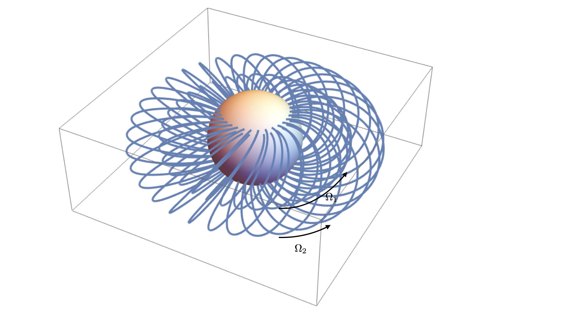
Figure 1: Rotating and twisted magnetosphere without light cylinder. Pictured are magnetic field lines for two flux surfaces. On each flux surface the magnetic field is twisted; in addition flux surfaces are rotating with spin frequency $\Omega$ decreasing as a function of maximal radius (equivalently, becoming smaller for smaller polar angles of the foot-points.

Note that in the cases when the eigen-problem cannot be satisfied, there may still be solutions with no light cylinder, but those solutions will be non-self-similar. Eventually, for large enough spin the light cylinder will be formed.

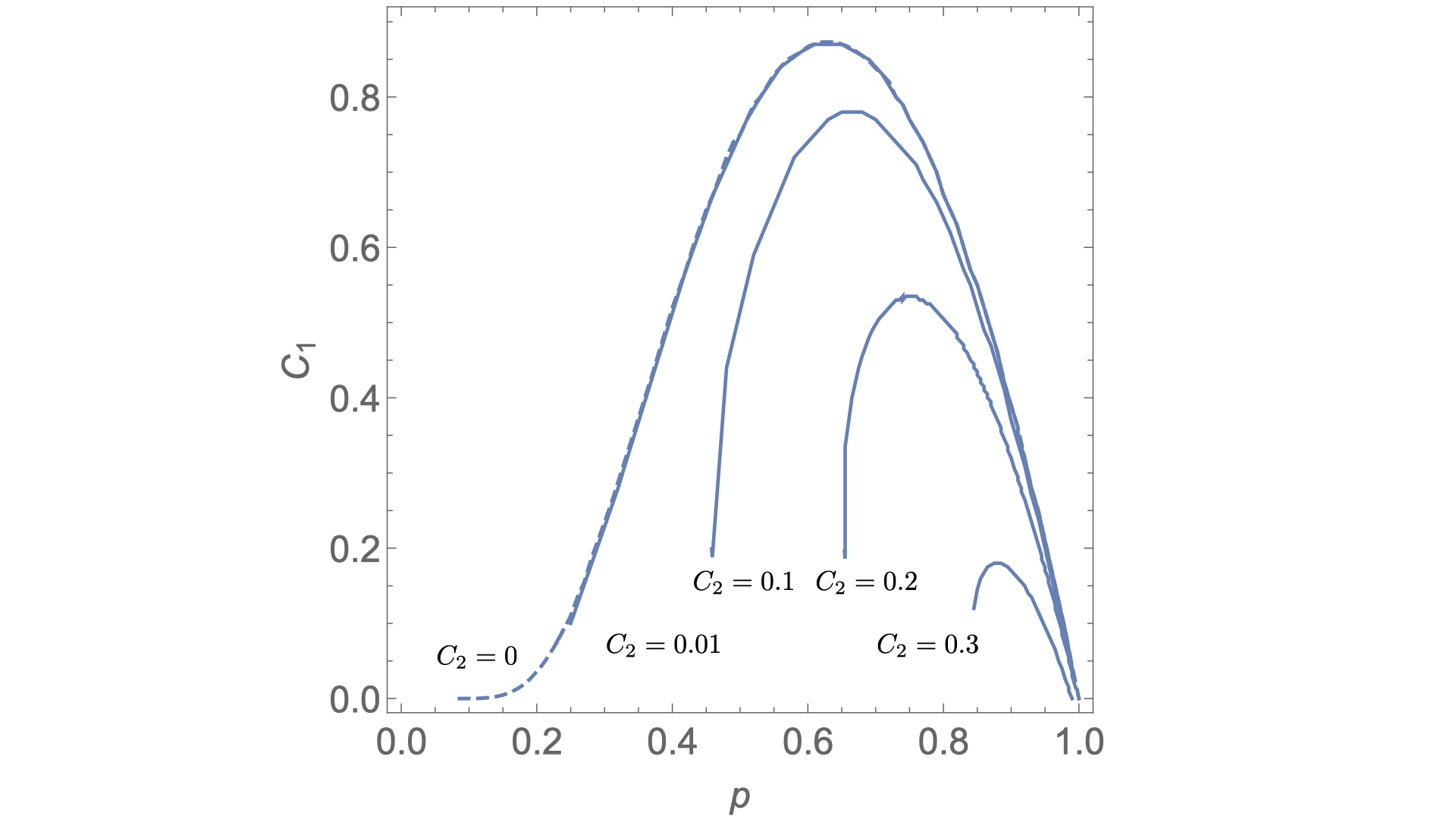
Figure 2: Radial power-law index $p$ as function of the twist parameter $C_{1}$ for different spins parameters. Dashed line, non-rotating is $C_{2}=0$. Other lines correspond to $C_{2}=0.01,\,0.1,\,0.2,\,0.3$ (top to bottom). Note that for cases when there are no self-similar solutions (e.g.  for $p$ smaller than some critical value for each $C_{2}\neq 0$) one may still a have no-light cylinder magnetosphere, but its structure is not self-similar.

In the case of untwisted magnetospheres, $C_{1}=0$, the maximal spin parameter is $C_{2}=0.34$, Fig. 3. We note that finite twists $C_{1}\neq 0$ allow for larger spins, Fig. 4.

For small twists the electromagnetic velocity is

$$\frac{{\bf E}\times{\bf B}}{B^{2}}\approx\left\{-\frac{2\sqrt{2}\sqrt{C_{1}}C_{2}\sin^{6}\theta\cos\theta}{5+3\cos(2\theta)},-\frac{\sqrt{2}\sqrt{C_{1}}C_{2}\sin^{7}\theta}{5+3\cos(2\theta)},2C_{2}\sin^{3}\theta\right\}$$ (9)

It is independent of the radius and changes sign at the equator. The Pointing flux $\propto r^{-2(2+p)}$ is zero at infinity: the pulsar does not spin down.

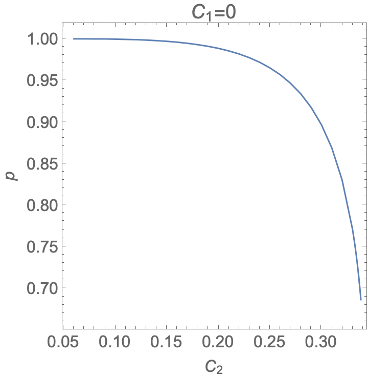
Figure 3: Radial power-law index $p$ as function of the rotation parameter $C_{2}$ for untwisted configuration $C_{1}=0$.

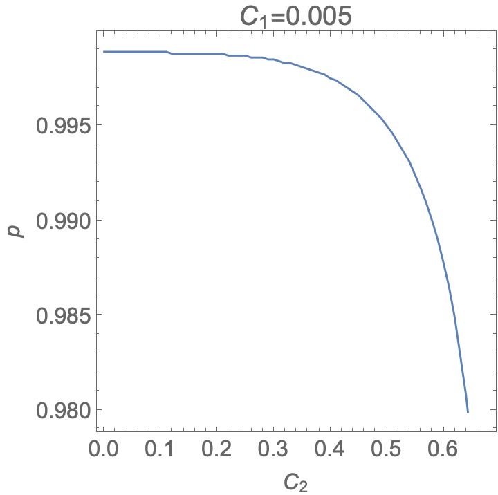
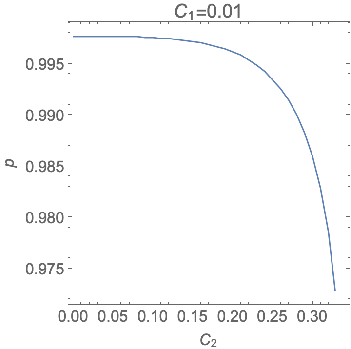
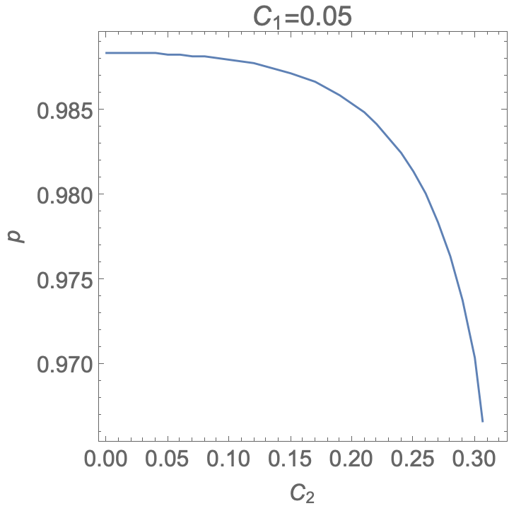
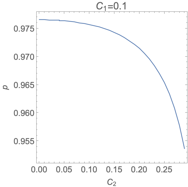
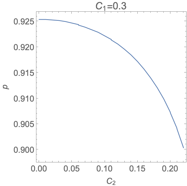
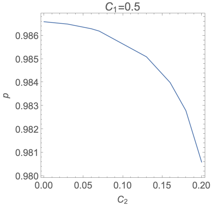
Figure 4: Radial power-law index $p$ as function of the spin parameter $C_{2}$ for different twist parameters. Beyond the plotted values the index $p$ falls down precipitously.

For each solution the angular velocity decreases with radius and increases with polar angle

$$\Omega=C_{2}\left(1+\frac{1}{p}\right)\frac{F(\mu)^{1/p}}{r}=\frac{R_{NS}}{r}{F(\mu)^{1/p}}\Omega_{0}$$ (10)

where typical value at the surface is

$$\Omega_{0}={C_{2}\left(1+\frac{1}{p}\right)}\frac{c}{R_{NS}}$$ (11)

(each flux surface rotates as a solid body.)

Azimuthal velocity is

$$v_{\phi}=\Omega r\sin\theta=(R_{NS}\Omega_{0})\sin\theta F^{1/p}$$ (12)

The locations of the light cylinder is determined by $v_{\phi}=c$. For the exemplary case of $C_{2}=0.1,C_{1}=0.66,p=0.79$ we have $\Omega_{0}=0.227$; the maximal value of $\Omega r\sin\theta$ equals $0.241\leq 1$. There is no light cylinder.

Generally, rotation leads to further (in addition to twisting) ”inflation” of field lines, Fig. 5. (We stress that inflation here occurs due to the rotation of a flux surface as a whole, not due to the shearing of the foot-points of a given field line).

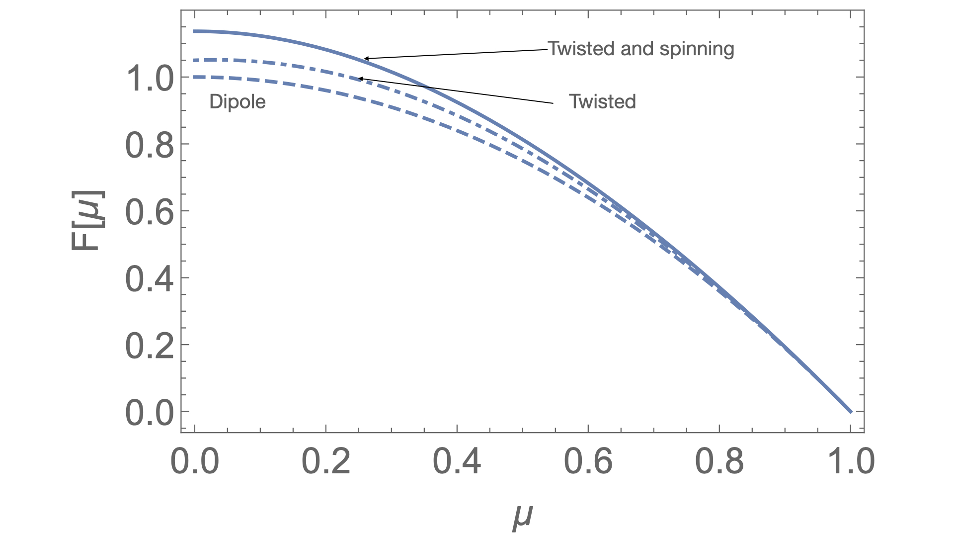
Figure 5: Example that both twist and rotation rotation leads to ”inflation” of field lines. Dashed line is for dipole $F=1-\mu^{2}$; dot-dashed is for twisted non-rotating case $C_{2}=0,C_{1}=0.66,p=0.867$, solid line is rotating case $C_{2}=0.1,C_{1}=0.66,p=0.79$ (same $C_{1}$ as non-rotating).

The electric potential

$$\Phi=C_{2}r^{-(1+p)}F^{1+1/p}$$ (13)

leads to distributed charge

$$\rho_{e}=\Delta\Phi\propto r^{-(3+p)}\approx\frac{\Omega_{0}B_{NS}}{4\pi c}\left(\frac{R_{NS}}{r}\right)^{-(3+p)}$$ (14)

electric field,

$${\bf E}=-\nabla\Phi\propto r^{-(2+p)}$$ (15)

Near the neutron star the radial component of the electric field integrated over the surface gives the central charge $Q_{c}$

$$Q_{c}\approx\frac{\Omega_{0}B_{NS}R_{NS}^{3}}{c}$$ (16)

Since for $r\rightarrow\infty$ $E_{r}\to 0$ faster than $1/r^{2}$, the total distributed charge equals the central charge.

3 Simulation

3.1 PHAEDRA code

PHAEDRA code (Parfrey et al., 2012) is a pseudo-spectral code developed specifically to study highly magnetized plasma regime, force-free electrodynamics, the vanishing-inertia limit of magnetohydrodynamics (Gruzinov, 1999; Komissarov, 2006)

The code solves Maxwell’s equations

$$\begin{array}[]{l}\frac{1}{c}{\partial_{t}\mathbf{B}}=-\nabla\times\mathbf{E}\\ \frac{1}{c}{\partial_{t}\mathbf{E}}=\nabla\times\mathbf{B}-\frac{4\pi}{c}\mathbf{J}\end{array}$$ (17)

supplemented by the force-free expression.

$$\rho\mathbf{E}+\mathbf{J}\times\mathbf{B}=0$$ (18)

The force free Ohm’s law is then

$$\frac{4\pi\mathbf{J_{FF}}}{c}=\frac{B\cdot\nabla\times\mathbf{B}-\mathbf{E}\cdot\nabla\times\mathbf{E}}{B^{2}}\mathbf{B}+\nabla\cdot\mathbf{E}\frac{\mathbf{E}\times\mathbf{B}}{\mathbf{B}^{2}}$$ (19)

Condition $\mathbf{E}.\mathbf{B}=0$ is satisfied by construction, while $\mathbf{B}^{2}-\mathbf{E}^{2}\geq 0$ is assumed (and checked at each step). The code uses a thin frictional absorbing layer next to the outer boundary. The code applies two spectral filters of 8th and 36th order, to maintain stability (Parfrey et al., 2012).

Our results further indicate that the code is very stable and efficient, and has low numerical dissipation. The full numerical grid is defined in axisymmetric spherical coordinates and composed of $N_{r}\times N_{\theta}$ cells along the radial and $\theta$ directions, respectively. The simulation zone in our work extends from the stellar surface $r_{min}=R_{NS}$ up to $r_{max}=100R_{NS}$.

The inner boundary is set as the radius of the star ($r=R_{NS}$) and the following conditions are strongly enforced at every Runge-Kutta substep.

$$\begin{array}[]{l}B_{r}=B_{r}(\theta)\\ E_{\theta}=-\Omega B_{r}\sin\theta\\ E_{\phi}=0\end{array}$$ (20)

3.2 Initialization

Analytical self-similar solutions, §2.1, are approximations: the system is generally non-self-similar (there is a special scale - the light cylinder). Thus, we do not expect the numerics to match exactly with analytics, just to follow the general trend. With this in mind, we initialize the simulation setup with analytical approximation for the structure of non-rotating twisted magnetospheres for small/mild twist parameter $C_{1}$, and the values of $C_{2}$ from the self-similar solution, Fig. 2. For small twists we can find analytical relation for the structure of non-rotating magnetosphere  by expanding near $p=1,\,C_{1}=0$ and the dipolar flux function (Lyutikov, 2013):

$$p=1-8C_{1}/35\mbox{}$$

$${F}=(1-\mu^{2})\left(1+{1\over 140}(1-\mu^{2})(17-5\mu^{2})C_{1}\right)\mbox{}$$

$$\mu=\cos\theta$$ (21)

In this approximation the flux magnetic field components and twist angle are given by

$$\frac{B_{r}}{B_{NS}}={2\mu\over\tilde{r}^{2+p}}\,\left(1+{3(13-18\mu^{2}+5\mu^{4})\over 140}C_{1}\right)\mbox{}$$

$$\frac{B_{\theta}}{B_{NS}}=p{\sqrt{1-\mu^{2}}\over\tilde{r}^{2+p}}\,\left(1+{(17-22\mu^{2}+5\mu^{4})C_{1}\over 140}\right)\mbox{}$$

$$\frac{B_{\phi}}{B_{NS}}={\sqrt{\frac{C_{1}p}{1+p}}\frac{(1-\mu^{2})^{3/2}}{\tilde{r}^{2+p}}}\mbox{}$$

$$\frac{j_{r}}{B_{NS}/{4\pi}}=2\sqrt{2}\mu(1-\mu^{2})\tilde{r}^{-3-p}\sqrt{C_{1}}\mbox{}$$

$$\frac{j_{\theta}}{B_{NS}/{4\pi}}=\sqrt{2}(1-\mu^{2})^{3/2}\tilde{r}^{-3-p}\sqrt{C_{1}}\mbox{}$$

$$\frac{j_{\phi}}{B_{NS}/{4\pi}}=(1-\mu^{2})^{5/2}\tilde{r}^{-3-p}C_{1}\mbox{}$$

$$\Delta\phi=\sqrt{2C_{1}}\mu_{fp}\mbox{}$$

$$\tilde{r}=\frac{r}{R_{NS}}$$ (22)

where $C_{1}$ is a twist parameter, $\mu_{fp}$ is the cosine of the polar angle of the northern foot point and $B_{NS}$ is the equatorial magnetic field.

3.3 Results

In order to demonstrate that the simulated magnetic field follows the radial scaling predicted by analytics, we plot a time slice of toroidal magnetic field $B_{\phi}$ at $\theta=\frac{\pi}{2}$ in Fig. 6 and try to fit it to $r^{-(2+p)}$. We see that the our radial scaling is in agreement with the analytics.

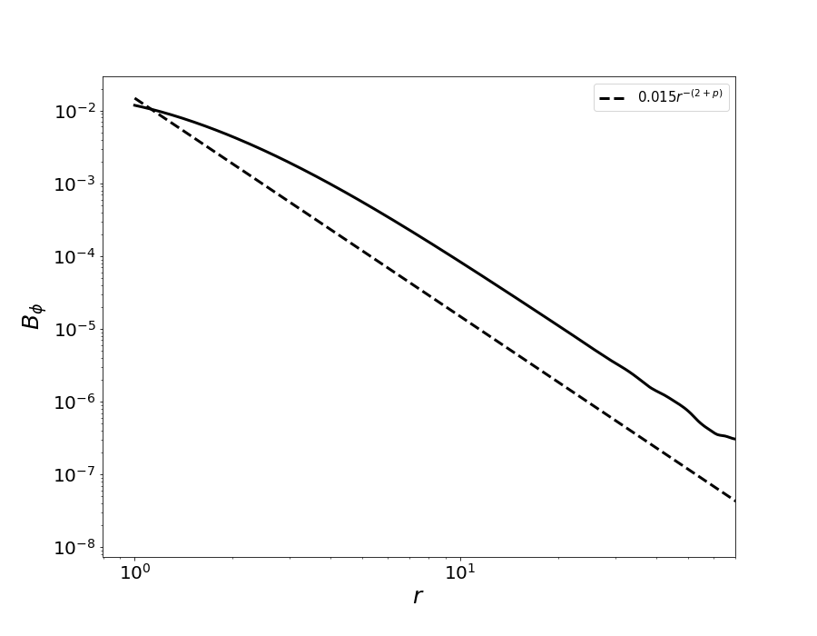
Figure 6: Time slice of toroidal magnetic field $B_{\phi}$ near the equator for $C_{2}=0.10,C_{1}=0.005,p=0.9989$. Solid line is our simulation results, dashed line is the theoretical expectation $r^{-(2+p)}$.

In Fig. 7 we plot the scaled azimuthal magnetic field, radial momentum, and the azimuthal velocity for three sets of $C_{1},C_{2}$. For $C_{1}=0.005\sim 0$ as evident in the top panel, the structure of the rotating magnetosphere clearly matches the analytical result: there are no open field lines, not radial Poynting flux, no energy losses. We see similar structure for the case of $C_{2}=0.1,C_{1}=0.66,p=0.79$ (twisted sheared configuration) in bottom panel.

For small $C_{2}$ all twisted configuration do not have a light cylinder ( first two panels in Fig. 7 and also bottom row in Fig. 8). When we increase the spin parameter $C_{2}$, the picture changed qualitatively, bottom panel in Fig. 7 (Also see middle row in Fig. 8).

$\hskip 30.00005ptC_{1}=0.005,C_{2}=0.10$

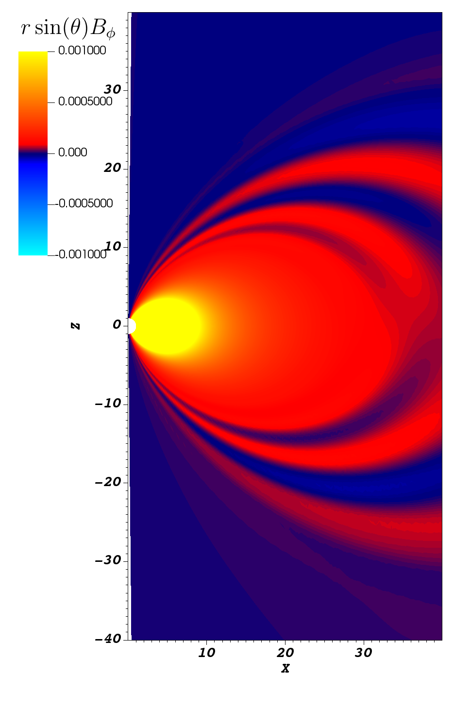
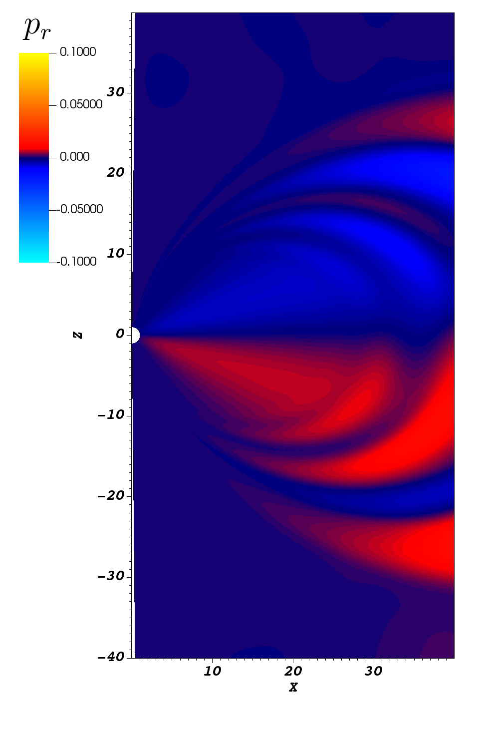
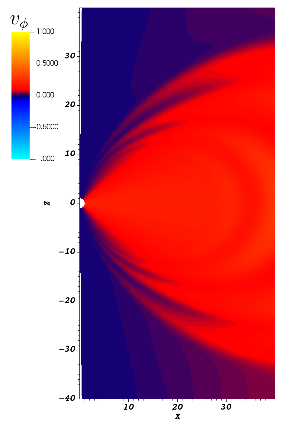
$\hskip 30.00005ptC_{1}=0.66,C_{2}=0.10$

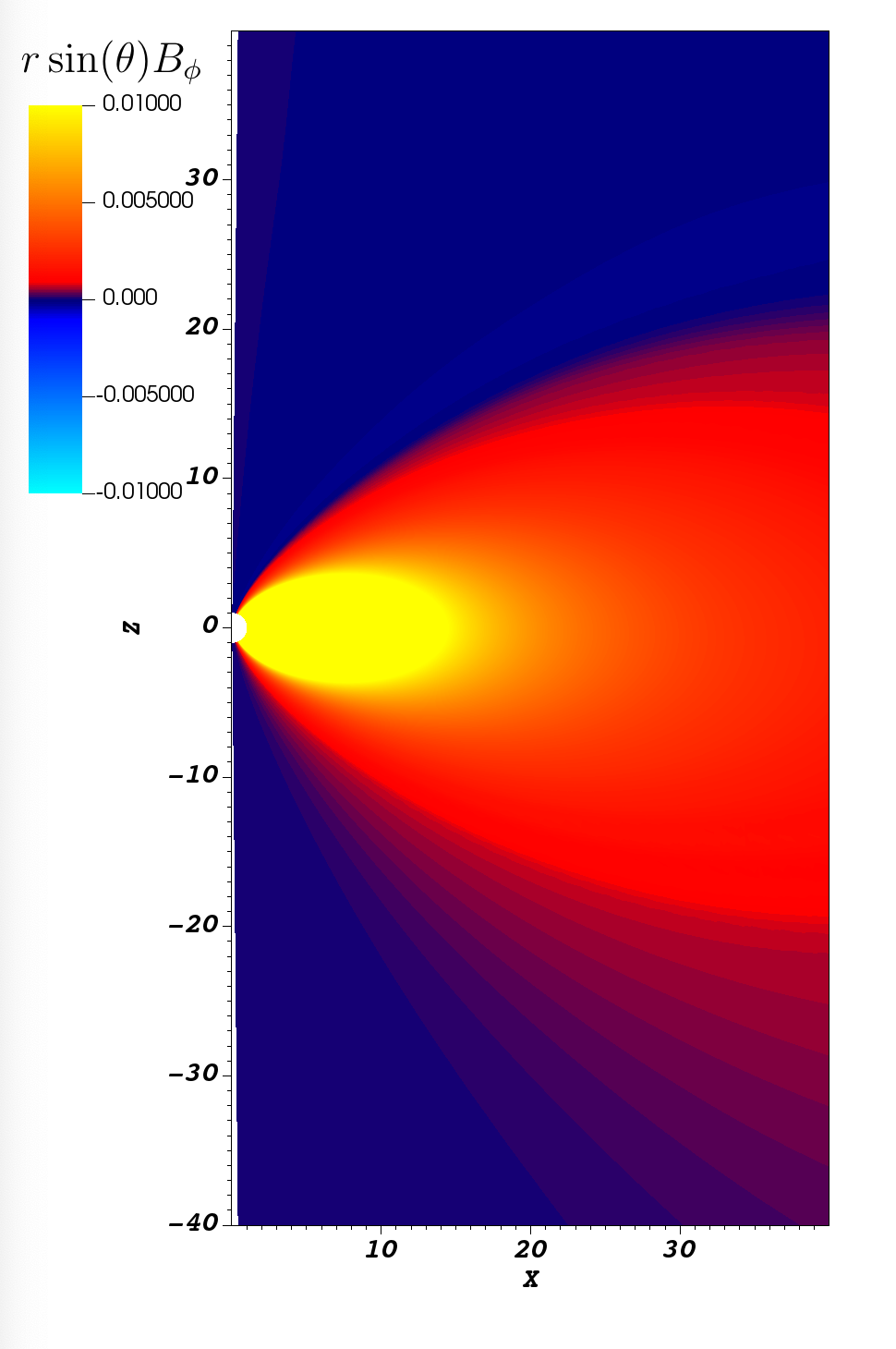
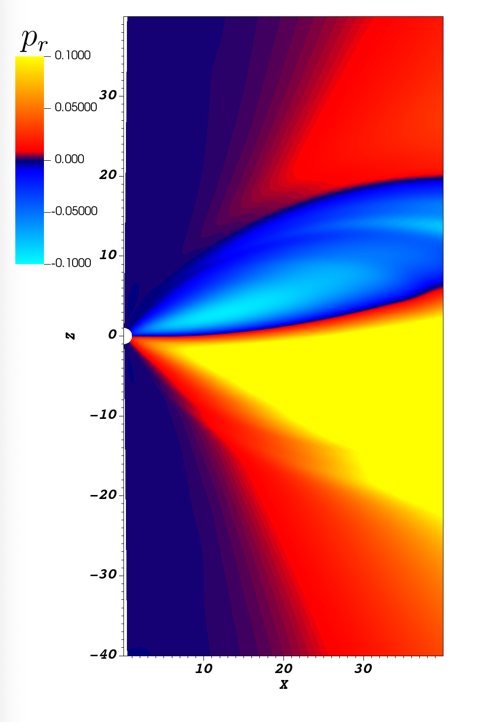
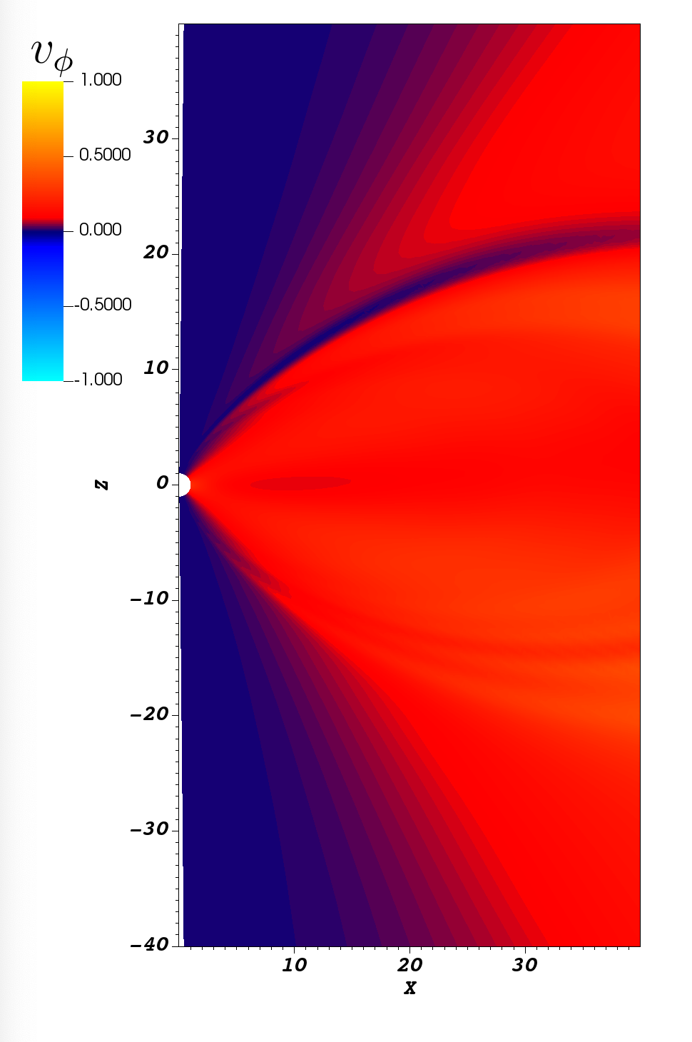
$\hskip 30.00005ptC_{1}=0.005,C{2}=0.20$

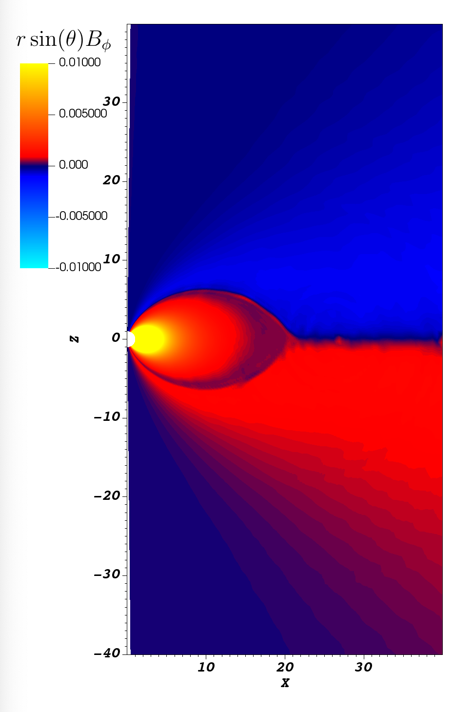
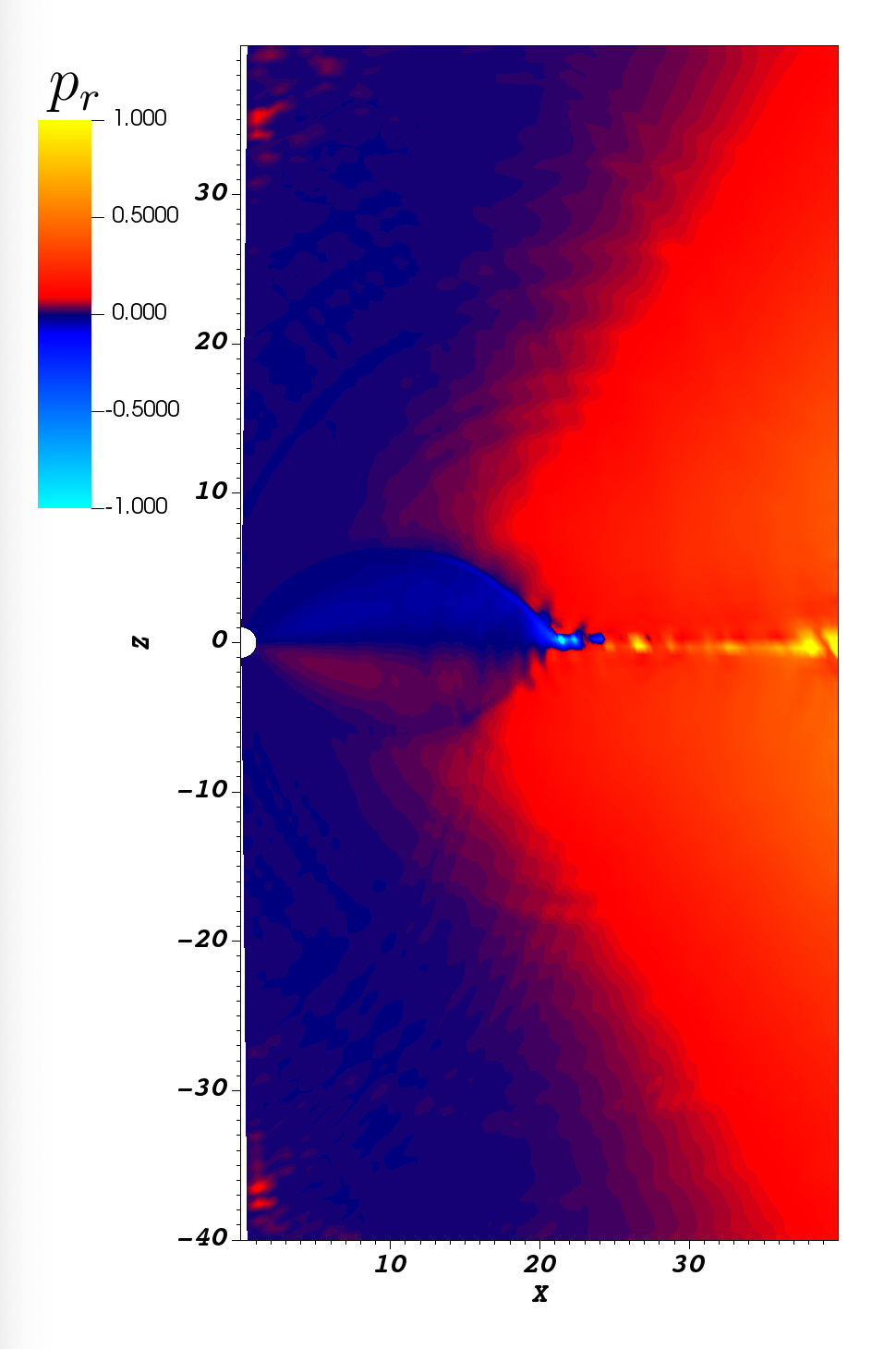
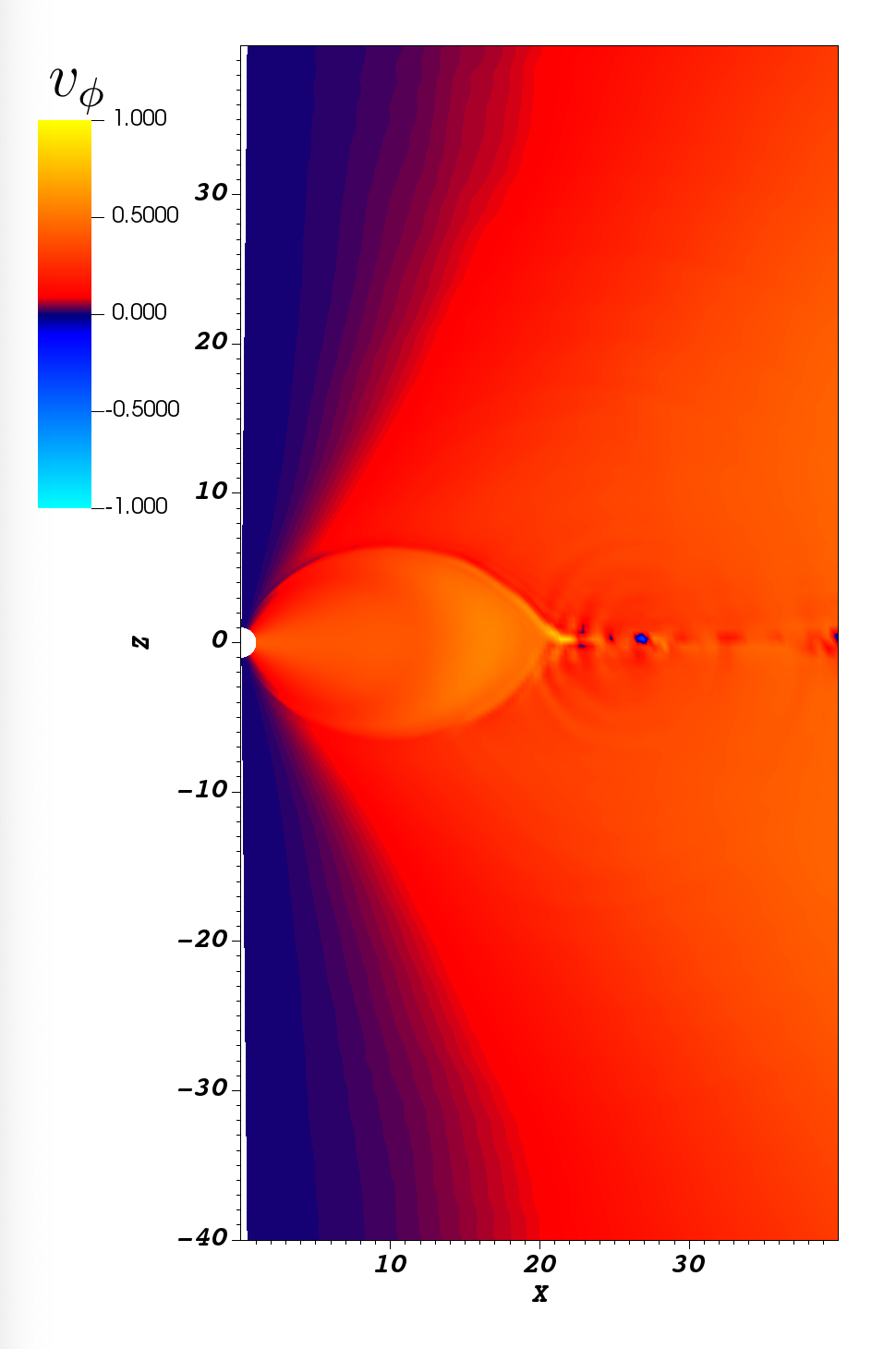
Figure 7: Zoomed-in time slice of our force-free simulation depicting toroidal magnetic field $r\sin(\theta)B_{\phi}$, radial momentum $p_{r}$ and toroidal velocity $v_{\phi}$ for the fiducial magnetosphere without light cylinder. In top panel we plot $C_{1}=0.005,C_{2}=0.10,p=0.9989$ case, middle panel is for $C_{1}=0.66,C_{2}=0.10,p=0.79$, bottom panel is for $C_{1}=0.05,C_{2}=0.20,p=0.9854$. The radial momentum is the ${\bf E}\times{\bf B}\propto C_{2}\sqrt{C_{1}}$ drift, Eq. (7). Since $\Omega\propto 1/r$, Eq. (10), azimuthal velocity $v_{\phi}$ remains approximately constant with radius, Eq. (9), top right panels. We don’t observe light cylinder in top two rows. At higher spin parameter $C_{2}=0.2,C_{1}=0.05,p=0.9854$ (lower row) the light cylinder can be clearly identified by the location of the Y-point. The wind is generated (this is especially clearly seen in radial momentum $p_{r}$, central panel.

To further verify the observations made in previous paragraphs, we plot scaled toroidal magnetic field for various permutations of $C_{1},C_{2}$ in Fig. 8,

From the figures it is clear that the presence of the light cylinder and wind depends strongly on $C_{2}$. For slow rotation $C_{2}=0.1$ (bottom row) there is no light cylinder. The light cylinder appears near $C_{2}\geq C_{2,crit}\approx 0.15$. (To guide an eye, formation of the wind requires light cylinder and the corresponding formation of a Y-point. Images with no Y-point imply no wind and no light cylinder.) A more precise critical value of $C_{2,crit}$ could not be determined: at the transition the light cylinder appears at large distances, reaching the absorbing layer next to the outer boundary). For larger $C_{2}\geq C_{2,crit}$ the light cylinder is located closer to the star. We restrict our simulations to $C_{2}\leq 0.3$. At this moment the light cylinder is located nearly at the star’s surface, but the relaxation time becomes very long (if compared with small $C_{2}$ cases).

$\hskip 30.00005ptC_{2}=0.2$

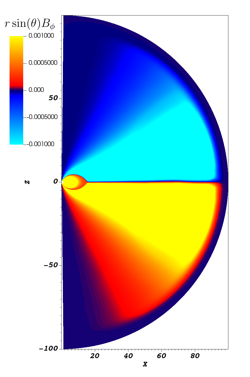
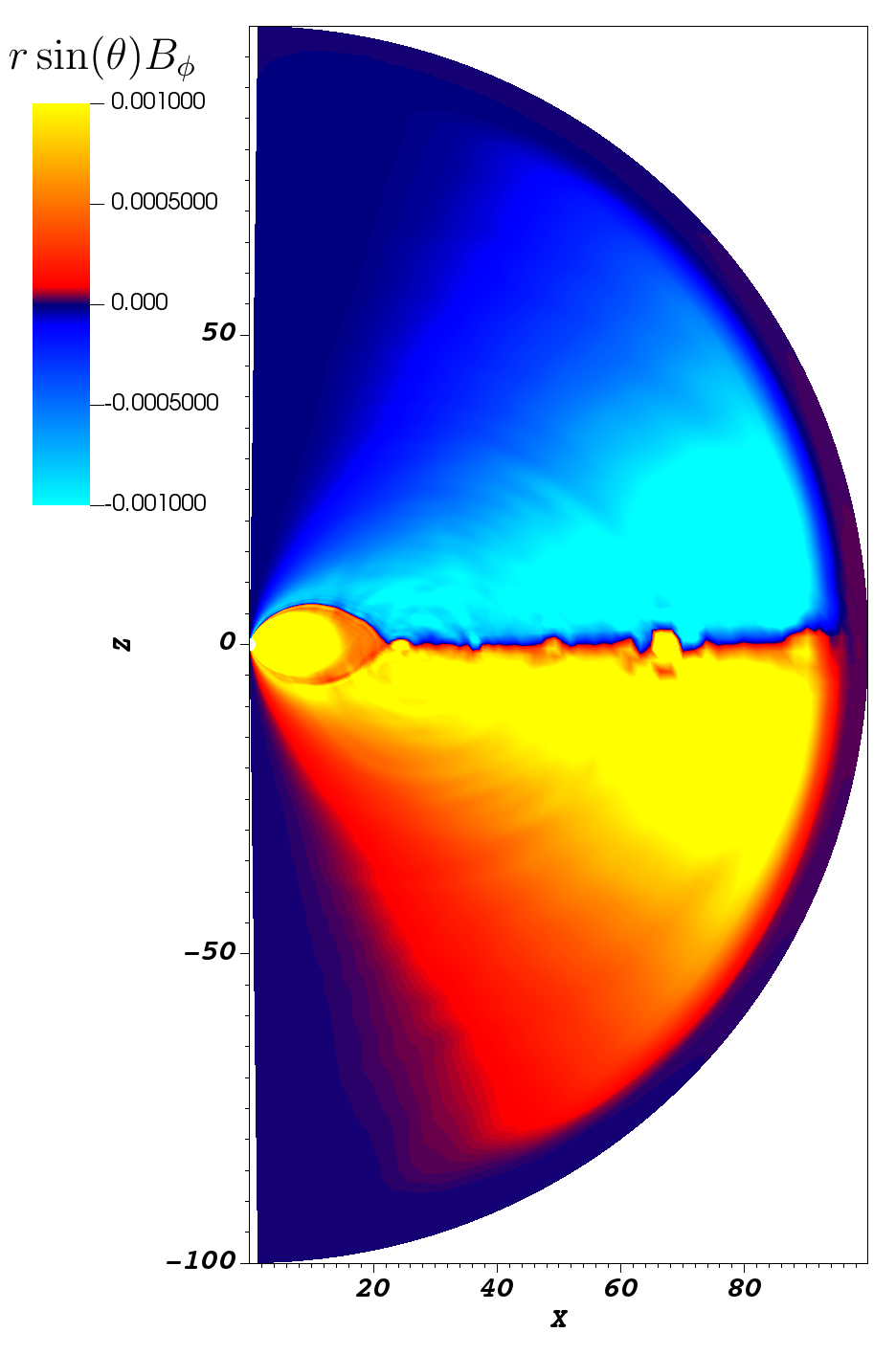
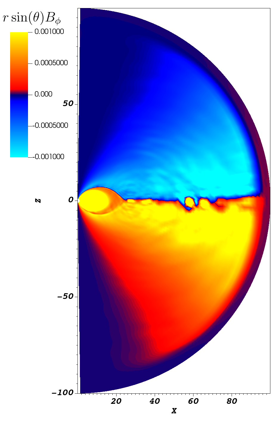
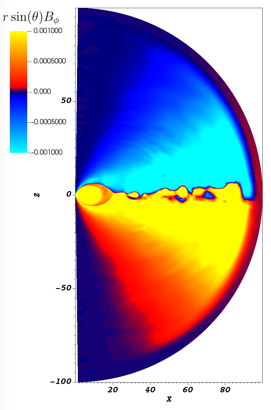
$\hskip 30.00005ptC_{2}=0.15$

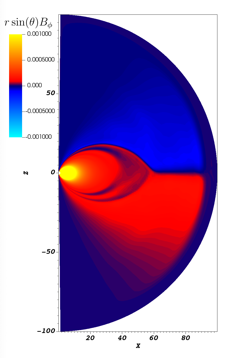
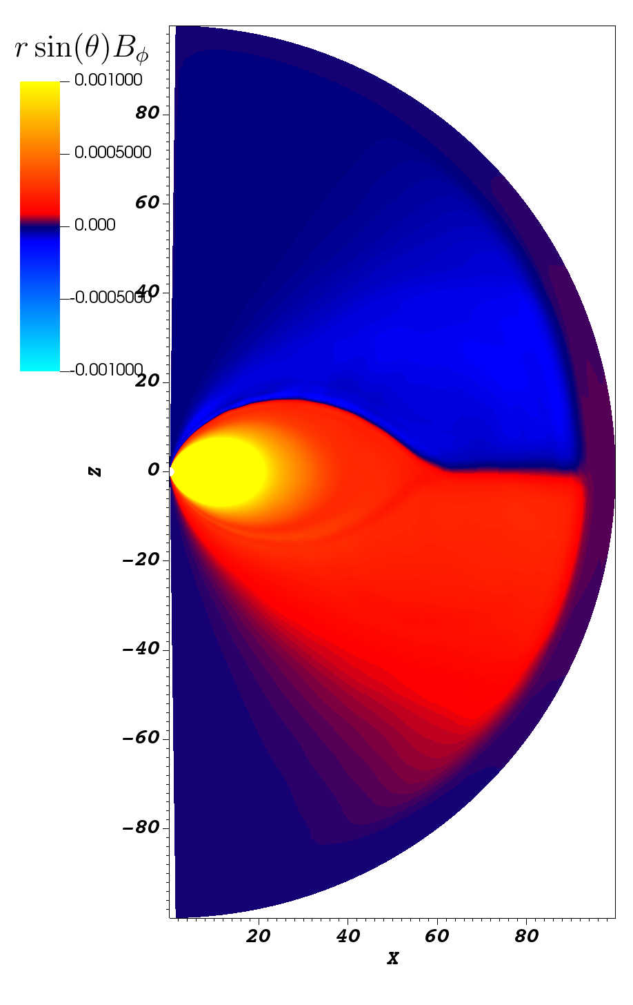
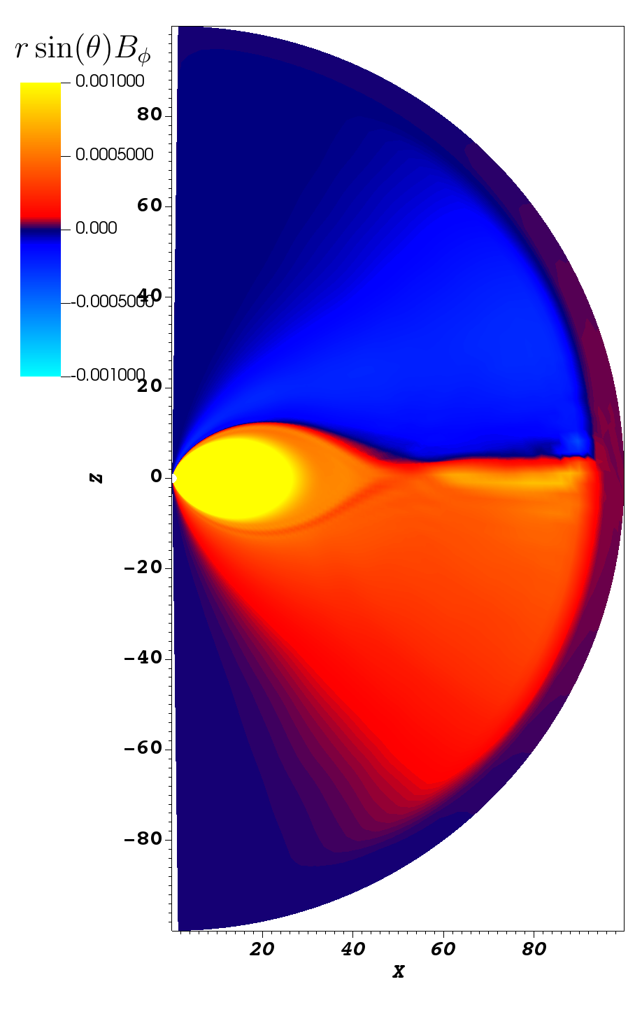
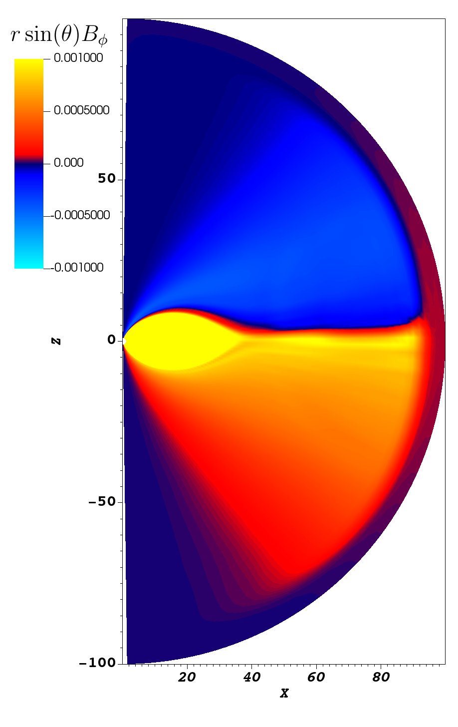
$\hskip 40.00006ptC_{2}=0.1$

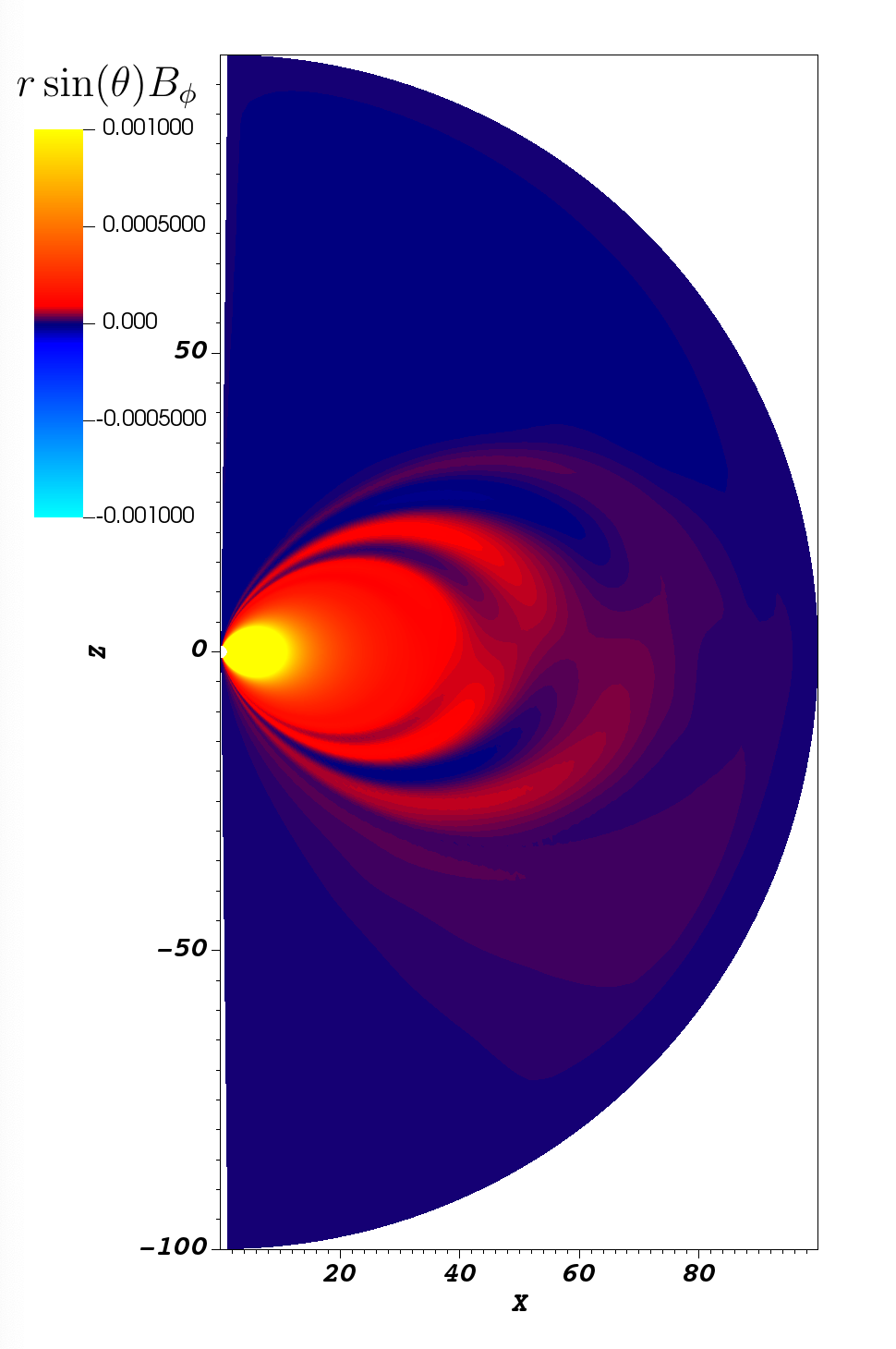
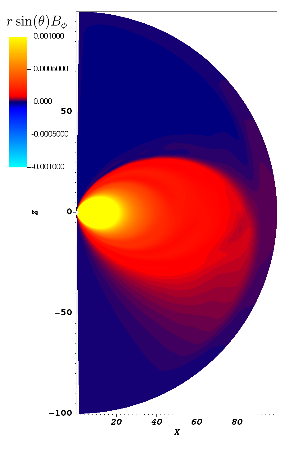
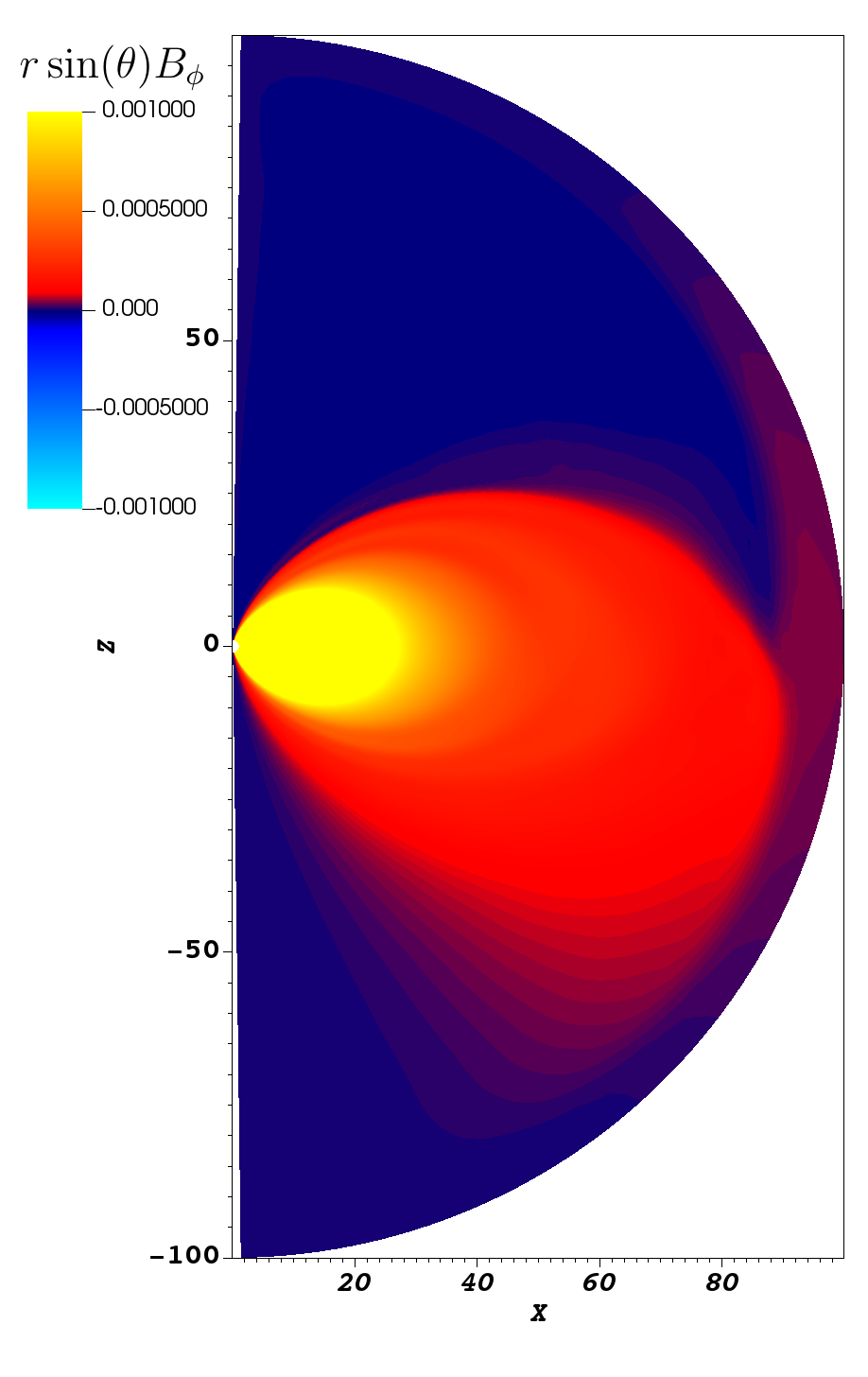
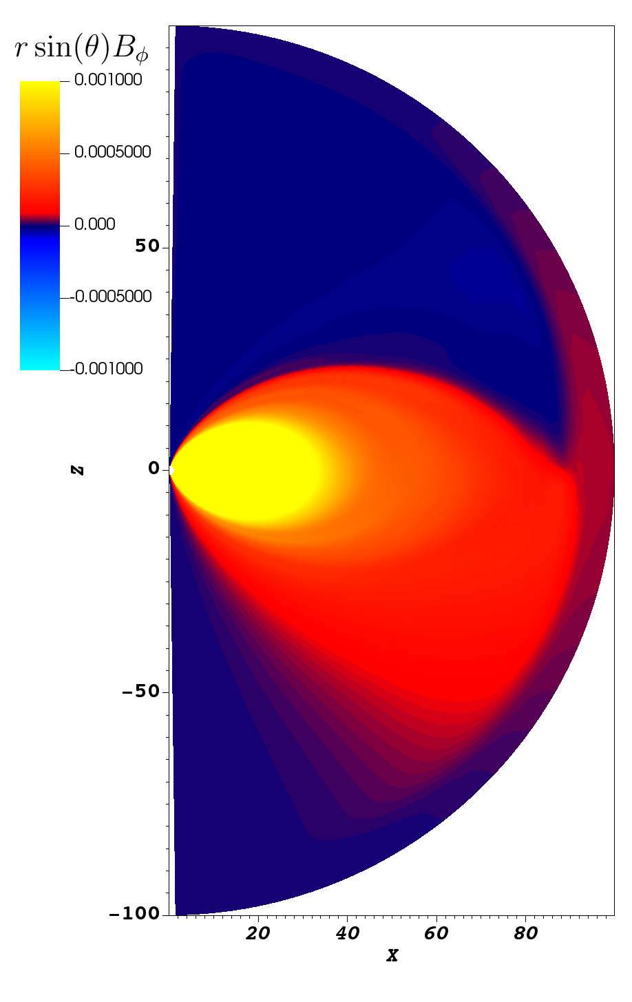
$C_{1}=0.01$

$C_{1}=0.1$

$C_{1}=0.2$

$C_{1}=0.3$

Figure 8: A mosaic of $r\sin(\theta)B_{\phi}$ for different twist rotation parameters $C_{1}$ and $C_{2}$. $C_{2}=0.2$ (top panel), $C_{2}=0.15$ (middle panel), and $C_{2}=0.1$ (bottom panel). $C_{1}=0.01,0.1,0.2,0.3$ from left to right for both panels at $t=30$, measured in light crossing time ${R_{NS}}{/c}$).

4 Discussion

We discuss an analytical model of a differentially rotating neutron stars with twisted magnetospheres. We find a new type of solutions without light cylinders. Such configuration could still be a pulsar, a rotating neutron star: it will be more like magnetar producing periodically modulated radio emission driven by magnetic reconnection (Lyutikov, 2002, 2020a), not by the rotational energy.

The present model is mostly mathematical. It requires that the twisting motion of the foot-points be comparable to the spin; and the spin shear must be of the particular shape, related to twist. It is a bit surprising that rotating magnetospheres can still be self-similar, since there is a special distance, the light cylinder. Our results indicate, that there is a special set of parameters without light cylinder, thus allowing for self-similar solution.

We see the value of the model in that, first, that it provides a clear analytical example of a new types of solutions of the pulsar equation: rotating yet non-spinning down configurations. Secondly, the model might have implication for numerical modeling of twisted, sheared and rotating magnetospheres of magnetars. Those types of models usually start with stationary neutron star, and then twist, shear and rotate it. Necessarily, in those simulations the twisting, shearing and the rotation rate must be similar, as the simulations are limited in their dynamic range: they have to deal with twisting rates similar, just somewhat smaller, to the rotation rate.

5 ACKNOWLEDGEMENTS

This work had been supported by NASA grants 80NSSC17K0757 and 80NSSC20K0910, NSF grants 1903332 and 1908590. We would like to thank Yiannis Contopoulos, Kyle Parfrey and Alexander Philippov for discussions.

6 Data availability

The data underlying this article will be shared on reasonable request to the corresponding author.

References

- Beskin (2009) Beskin, V. S. 2009, MHD Flows in Compact Astrophysical Objects: Accretion, Winds and Jets
- Beskin et al. (1988) Beskin, V. S., Gurevich, A. V., & Istomin, I. N. 1988, Ap&SS, 146, 205
- Contopoulos et al. (1999) Contopoulos, I., Kazanas, D., & Fendt, C. 1999, ApJ, 511, 351
- Goldreich & Julian (1969) Goldreich, P. & Julian, W. H. 1969, ApJ, 157, 869
- Goldreich & Reisenegger (1992) Goldreich, P. & Reisenegger, A. 1992, ApJ, 395, 250
- Gourgouliatos et al. (2015) Gourgouliatos, K. N., Kondić, T., Lyutikov, M., & Hollerbach, R. 2015, MNRAS, 453, L93
- Grad (1967) Grad, H. 1967, Physics of Fluids, 10, 137
- Gruzinov (1999) Gruzinov, A. 1999, ArXiv Astrophysics e-prints
- Gruzinov (2005) —. 2005, Phys. Rev. Lett., 94, 021101
- Komissarov (2006) Komissarov, S. S. 2006, MNRAS, 367, 19
- Lynden-Bell & Boily (1994) Lynden-Bell, D. & Boily, C. 1994, MNRAS, 267, 146
- Lyutikov (2002) Lyutikov, M. 2002, ApJ, 580, L65
- Lyutikov (2006) —. 2006, MNRAS, 367, 1594
- Lyutikov (2011) —. 2011, Phys. Rev. D, 83, 124035
- Lyutikov (2013) —. 2013, arXiv e-prints, arXiv:1306.2264
- Lyutikov (2015) —. 2015, MNRAS, 447, 1407
- Lyutikov (2020a) —. 2020a, arXiv e-prints, arXiv:2006.16029
- Lyutikov (2020b) —. 2020b, Journal of Plasma Physics, 86, 905860210
- Michel (1973) Michel, F. C. 1973, ApJ, 180, L133
- Parfrey et al. (2012) Parfrey, K., Beloborodov, A. M., & Hui, L. 2012, MNRAS, 423, 1416
- Parfrey et al. (2013) —. 2013, ApJ, 774, 92
- Scharlemann & Wagoner (1973) Scharlemann, E. T. & Wagoner, R. V. 1973, ApJ, 182, 951
- Shafranov (1966) Shafranov, V. D. 1966, Reviews of Plasma Physics, 2, 103
- Spitkovsky (2006) Spitkovsky, A. 2006, ApJ, 648, L51
- Thompson et al. (2002) Thompson, C., Lyutikov, M., & Kulkarni, S. R. 2002, ApJ, 574, 332
- Wood et al. (2014) Wood, T. S., Hollerbach, R., & Lyutikov, M. 2014, Physics of Plasmas, 21, 052110