Accumulation of magnetoelastic bosons in yttrium iron garnet: kinetic theory and wave vector resolved Brillouin light scattering

Abstract

We derive and solve quantum kinetic equations describing the accumulation of magnetoelastic bosons in an overpopulated magnon gas realized in a thin film of the magnetic insulator yttrium iron garnet. We show that in the presence of a magnon condensate, there is a non-equilibrium steady state in which incoherent magnetoelastic bosons accumulate in a narrow region in momentum space for energies slightly below the bottom of the magnon spectrum. The results of our calculations agree quite well with Brillouin light scattering measurements of the stationary non-equilibrium state of magnons and magnetoelastic bosons in yttrium iron garnet.

I Introduction

The theoretical investigation of magnon-phonon interactions in magnetic insulators was initiated by Abrahams and Kittel Abrahams52 in 1952. Over the years the interest in this topic has waned and often the effect of the phonons on magnons has been taken into account only implicitly by assuming that phonons merely serve as a thermal bath and an energy sink for the magnons. Recently magnon-phonon interactions have attracted renewed interest in the field of spintronics Bozhko20 where one can now study phenomena which are dominated by the magnetoelastic coupling.Kamra14 ; Rueckriegel14 ; Ogawa15 ; Kikkawa16 ; Takahashi16 ; Baryakhtar17 ; Ramos19 ; Rueckriegel20 Of particular interest are magnetoelastic bosons which emerge because of the hybridization of magnons with phonons and as such combine properties of both. For example, in a recent series of experiments, Bozhko17 ; Frey21 the spontaneous accumulation of magnetoelastic bosons during the thermalization of an overpopulated magnon gas in the magnetic insulator yttrium iron garnet (YIG) was observed by Brillouin light scattering spectroscopy. While a phenomenological explanation of this observation in terms of a bottleneck accumulation effect was already provided by the authors of Ref. [Bozhko17, ], important questions about the nature of the accumulation remain open. For example, it is not clear whether the accumulation in the magnetoelastic mode is coherent. Moreover, in addition to the magnetoelastic accumulation, in the experiment a magnon condensate at the bottom of the magnon spectrum was also observed. As the magnon condensate and the magnetoelastic boson are energetically nearly degenerate, this raises the question of the importance of interactions between these different types of modes.

The theory of magnons, phonons, and hybrid magnetoelastic bosons in YIG films is already well-developed, see for example Refs. [Kalinkos86, ; Kreisel09, ; Rueckriegel14, ]. In the present work, we go beyond this established theory by developing a kinetic theory for the coupled magnon-phonon system which allows us to gain a complete microscopic understanding of the physical processes leading to the accumulation of magnetoelastic bosons in YIG Bozhko17 ; Frey21 . To this end, we derive quantum kinetic equations for the incoherent distribution functions and condensate amplitudes of the magnetoelastic bosons. We then solve the kinetic equations numerically to obtain a non-equilibrium steady state that displays the magnetoelastic accumulation. In the experimental section of this work, we present new wave vector resolved Brillouin light scattering results for the magnetoelastic accumulation in YIG which are in good agreement with our theoretical predictions.

The rest of this work is organized as follows: In Sec. II, we briefly review the theory of magnons and phonons in thin YIG films; in particular, we discuss the magnetoelastic modes and the relevant interaction vertices. The quantum kinetic equations describing the dynamics of the coupled magnon-phonon system are derived and self-consistently solved in Sec. III; we also compare our theoretical results with new Brillouin light scattering measurements. In the concluding Sec. IV we briefly summarize our results. Finally, in three appendices we present technical details of the derivation of the magnon-phonon Hamiltonian in YIG and of the derivation of the relevant collision integrals using an unconventional method based on a systematic expansion in powers of connected equal-time correlations. Fricke97 ; Hahn21

II Magnetoelastic bosons in YIG

II.1 Magnons

At room temperature, the low-energy magnetic properties of YIG can be described by the following effective quantum spin Hamiltonian, Cherepanov93 ; Tupitsyn08 ; Kreisel09

$$\mathcal{H}_{m}=-\frac{1}{2}\sum_{ij}\sum_{\alpha\beta}\left(J_{ij}\delta^{\alpha\beta}+D_{ij}^{\alpha\beta}\right)S_{i}^{\alpha}S_{j}^{\beta}-h\sum_{i}S_{i}^{z},$$ (1)

where the indices $i,j=1,\dots,N$ label the sites $\bm{R}_{i}$ and $\bm{R}_{j}$ of a simple cubic lattice with spacing $a\approx 12.376\,\mathrm{\r{A}}$, and $\alpha,\beta\in\{x,\,y,\,z\}$ denote the Cartesian components of the spin operators $\bm{S}_{i}$ localized at lattice sites $\bm{R}_{i}$. The ferromagnetic exchange coupling $J_{ij}=J\left(\bm{R}_{i}-\bm{R}_{j}\right)$ has the value $J\approx 3.19\,{\rm K}$ if the lattice sites $\bm{R}_{i}$ and $\bm{R}_{j}$ are nearest neighbors and vanishes otherwise. Finally, the dipole-dipole interaction tensor is

$$D_{ij}^{\alpha\beta}=\left(1-\delta_{ij}\right)\frac{\mu^{2}}{\left|\bm{R}_{ij}\right|^{3}}\left[3\hat{{R}}_{ij}^{\alpha}\hat{{R}}_{ij}^{\beta}-\delta^{\alpha\beta}\right],$$ (2)

where $\bm{R}_{ij}=\bm{R}_{i}-\bm{R}_{j}$ and $\hat{\bm{R}}_{ij}=\bm{R}_{ij}/\left|\bm{R}_{ij}\right|$ is the corresponding unit vector. The magnetic moment is denoted by $\mu=2\mu_{B}$ where $\mu_{B}$ is the Bohr magneton. The external magnetic field $\bm{H}=H\bm{e}_{z}$ is assumed to be applied in $z$-direction (the classical ground state is then a saturated ferromagnet with macroscopic magnetization also pointing in $z$-direction) and we denote by $h=\mu H$ the corresponding Zeeman energy. Having fixed $\mu$ as described above, we may use the value of the room-temperature saturation magnetization $4\pi M_{S}=1750\,{\rm G}$ of YIG to determine the effective spin $S=M_{s}a^{3}/\mu\approx 14.2$ of our spin model Tupitsyn08 ; Kreisel09 . This large value of $S$ allows us to bosonize the spin Hamiltonian (1) via the Holstein-Primakoff transformation Holstein40 and expand the resulting effective boson Hamiltonian with respect to the small parameter $1/S$. As described in Appendix A, the quadratic part of the bosonic Hamiltonian is then diagonalized by transforming to momentum space and a canonical (Bogoliubov) transformation. Dropping unimportant constants, this procedure yields the following quadratic magnon Hamiltonian for YIG,

$$\mathcal{H}_{m}^{(2)}=\sum_{\bm{k}}\epsilon_{\bm{k}}b^{\dagger}_{\bm{k}}b_{\bm{k}},$$ (3)

where $b^{\dagger}_{\bm{k}}$ creates a magnon with momentum ${\bm{k}}$ and energy dispersion $\epsilon_{\bm{k}}$. In the thin film geometry shown in Fig. 1, it is sufficient to work with an effective two-dimensional model in order to describe the lowest magnon band of YIG.

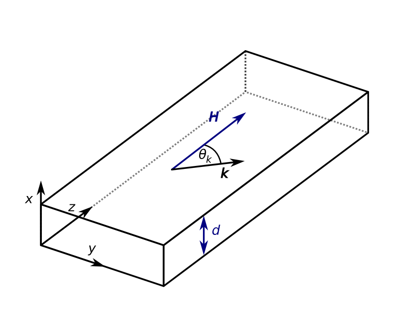
Figure 1: Geometry of a thin YIG film with thickness $d$ in the presence of a uniform external magnetic field $\bm{H}=H\bm{e}_{z}$ parallel to the plane of the film. In this work we consider only the lowest, uniform thickness modes with in-plane wave vectors ${\bm{k}}=\bm{e}_{z}|{\bm{k}}|\cos\theta_{\bm{k}}+\bm{e}_{y}|{\bm{k}}|\sin\theta_{\bm{k}}$.

Then the long-wavelength dispersion is well approximated by Kreisel09 ; Tupitsyn08 ; Kalinkos86 ; Hillebrands90

$$\epsilon_{\bm{k}}= \left[h+\rho_{s}{\bm{k}}^{2}+\left(1-f_{\bm{k}}\right)\Delta\sin^{2}\theta_{\bm{k}}\right]^{1/2}$$

$$\times\left[h+\rho_{s}{\bm{k}}^{2}+f_{\bm{k}}\Delta\right]^{1/2}.$$ (4)

Here, $\theta_{\bm{k}}$ is the angle between the magnetic field and the wave vector ${\bm{k}}$ (see Fig. 1), $\rho_{s}=JSa^{2}$ and $\Delta=4\pi M_{s}$ are the spin stiffness and the dipolar energy scale respectively, and

$$f_{\bm{k}}=\frac{1-e^{-|{\bm{k}}|d}}{|{\bm{k}}|d}$$ (5)

is the form factor for a film of thickness $d$. The magnon dispersion (4) is shown in Fig. 2 for momenta parallel and perpendicular to the magnetic field and experimentally relevant parameters. Note that in the long-wavelength regime probed by experiments Bozhko17 ; Frey21 which we aim to describe, the magnon dispersion (4) of YIG is rather flat. As a consequence, all decay processes which do not conserve the number of participating magnons are forbidden by energy conservation. Thus, there is an (approximate) $U(1)$ symmetry for low-energy magnons in YIG, which is one of the reasons that magnon condensation is possible in the first place. Therefore we retain only the number-conserving two-body magnon-magnon interaction

$$\mathcal{H}_{m}^{(4)} = \frac{1}{N}\sum_{{\bm{k}}_{1}\dots\bm{k}_{4}}\delta_{{\bm{k}}_{1}+\dots+{\bm{k}}_{4},0}\frac{1}{4}U_{{\bm{k}}_{1},{\bm{k}}_{2};{\bm{k}}_{3},{\bm{k}}_{4}}$$ (6)

$$\times b^{\dagger}_{-{\bm{k}}_{1}}b^{\dagger}_{-{\bm{k}}_{2}}b_{{\bm{k}}_{3}}b_{{\bm{k}}_{4}},$$

where the interaction vertex $U_{{\bm{k}}_{1},{\bm{k}}_{2};{\bm{k}}_{3},{\bm{k}}_{4}}$ is explicitly given in Eq. (LABEL:eq:vertex4) of Appendix A.

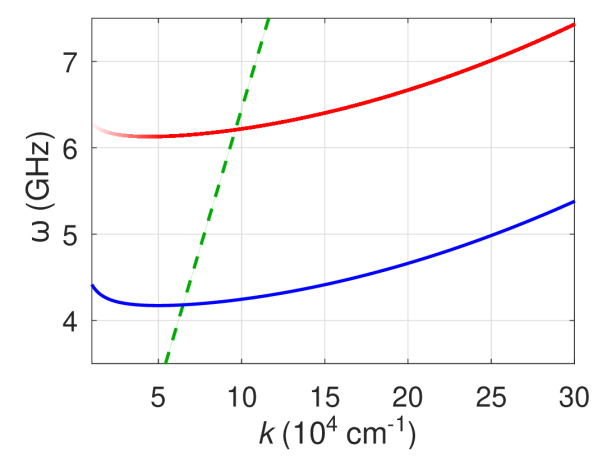
Figure 2: Magnon dispersion $\epsilon_{\bm{k}}$ as a function of wave vector $k=|{\bm{k}}|$ of a YIG film with thickness $d=6.7\,\mu{\rm m}$ in a magnetic field $H=145\,{\rm mT}$ for momenta parallel (blue) and perpendicular (red) to the magnetic field. Note that for very small momenta perpendicular to the field, the magnon dispersion relation (4) exhibits an unphysical negative slope, which we indicate by the shading of the red curve footnote_DE . We also show the dispersion $\omega_{{\bm{k}}\bot}=c_{\bot}|{\bm{k}}|$ (dashed green) of the transverse acoustic phonon mode in YIG.

II.2 Phonons and magnetoelastic hybridization in YIG

So far, we have considered only the magnon subsystem. In order to address the accumulation of magnetoelastic bosons, we should also take the phonons in YIG into account. At long wavelengths, the three relevant acoustic phonon branches of YIG are described by the following quadratic phonon Hamiltonian,

$$\mathcal{H}_{p}^{(2)}=\sum_{{\bm{k}}\lambda}\omega_{{\bm{k}}\lambda}\left(a_{{\bm{k}}\lambda}^{\dagger}a_{{\bm{k}}\lambda}+\frac{1}{2}\right),$$ (7)

where $a_{{\bm{k}}\lambda}^{\dagger}$ creates a phonon with momentum ${\bm{k}}$, polarization $\lambda$, and energy $\omega_{{\bm{k}}\lambda}=c_{\lambda}|{\bm{k}}|$, where $c_{\lambda}$ are the phonon velocities. It is well known Gurevich96 ; Gilleo58 that in YIG there are two degenerate transverse ($\lambda=\bot 1,\,\bot 2$) phonon modes with phonon velocity $c_{\bot 1}=c_{\bot 2}\equiv c_{\bot}=3.843\times 10^{5}\,\mathrm{cm}/\mathrm{s}$, and one longitudinal ($\lambda=\|$) mode with velocity $c_{\|}=7.209\times 10^{5}\,\mathrm{cm}/\mathrm{s}$. Interactions between the phonons can be safely ignored because of the large mass density $\rho=5.17\,\mathrm{g}/\mathrm{cm}^{3}$ of YIG. Gurevich96 The transverse phonon dispersion $\omega_{{\bm{k}}\bot}$ is shown in Fig. 2 as a dashed green line.

The coupling between the magnons and the phonons arises both from the dependence of the exchange interaction on the ionic positions as well as from relativistic effects involving the charge degrees of freedom which cannot be taken into account directly within an effective spin model. As the latter is usually dominant in collinear magnets at low energies,Gurevich96 we opt to derive the magnon-phonon interactions by quantizing the phenomenological expression for the classical magnetoelastic energy. This strategy was pioneered by Abrahams and Kittel Abrahams52 and more recently adopted in Ref. [Rueckriegel14, ]. At long wavelengths, the relevant contribution to the classical magnetoelastic energy is

$$E_{\rm me}=\frac{n}{M_{s}^{2}}\int d^{3}r\sum_{\alpha\beta}B^{\alpha\beta}M^{\alpha}(\bm{r})M^{\beta}(\bm{r})X^{\alpha\beta}(\bm{r}),$$ (8)

where $\bm{M}(\bm{r})$ is the local magnetization, $X^{\alpha\beta}(\bm{r})$ is the symmetric strain tensor, $n=a^{-3}$ is the number density of magnetic ions, and $B^{\alpha\beta}$ are phenomenological magnetoelastic constants. For a cubic lattice, these constants can be written as $B^{\alpha\beta}=\delta^{\alpha\beta}B_{\parallel}+(1-\delta^{\alpha\beta})B_{\bot}$, where $B_{\|}=47.8\,\mathrm{K}$ and $B_{\bot}=95.6\,\mathrm{K}$ for YIG Gurevich96 ; Eggers63 ; Hansen73 . The magnetoelastic energy (8) can then be quantized by replacing $\bm{M}(\bm{r}=\bm{R}_{i})\to\mu n\bm{S}_{i}$ and expanding the strain tensor $X^{\alpha\beta}(\bm{r})$ in terms of the phonon operators $a_{{\bm{k}}\lambda}$ and $a_{{\bm{k}}\lambda}^{\dagger}$. This procedure, outlined in Appendix. B and discussed in detail in Ref. Rueckriegel14, , yields to lowest order in $1/S$ the following Hamiltonian for the hybridization of magnons and phonons,

$$\mathcal{H}_{mp}^{(2)}=\frac{1}{2}\sum_{{\bm{k}}\lambda}\Gamma_{{\bm{k}}\lambda}\left(a_{-{\bm{k}}\lambda}+a_{{\bm{k}}\lambda}^{\dagger}\right)b_{\bm{k}}+{\rm h.c.},$$ (9)

where h.c. denotes the hermitian conjugate, and the hybridization vertices $\Gamma_{{\bm{k}}\lambda}$ are given explicitly in Eqs. (B6) and (B7) of Appendix B. Higher order magnon-phonon interactions open up additional decay channels.Rueckriegel14 ; Streib19 However, for YIG films the contribution of these processes is generally several orders of magnitude smaller than the contribution of the magnon-magnon interaction (6) at long wavelengths Demokritov06 ; Rueckriegel14 ; Streib19 , which justifies neglecting them.

In the following, we will focus solely on the transverse phonon branches and drop the longitudinal ones, because in thin YIG films only the two transverse branches hybridize with the magnons in the experimentally relevant region Frey21 ; Rueckriegel14 . To describe the magnetoelastic modes, we may furthermore neglect the non-resonant terms $a_{-{\bm{k}}\lambda}b_{\bm{k}}$ and $a_{-{\bm{k}}\lambda}^{\dagger}b_{\bm{k}}^{\dagger}$ in the hybridization Hamiltonian (9) as discussed in Refs. [Takahashi16, ; Bozhko17, ]. In this approximation, the quadratic Hamiltonian

$${\cal H}^{(2)}={\cal H}_{m}^{(2)}+{\cal H}_{p}^{(2)}+{\cal H}_{mp}^{(2)}$$ (10)

of the coupled magnon-phonon system can be diagonalized by the unitary transformation

$$\left(\begin{matrix}b_{\bm{k}}\\ a_{{\bm{k}}\bot 1}\\ a_{{\bm{k}}\bot 2}\end{matrix}\right)=\left(\begin{matrix}\bm{\phi}_{{\bm{k}}+},\bm{\phi}_{{\bm{k}}-},\bm{\phi}_{{\bm{k}}p}\end{matrix}\right)\left(\begin{matrix}\psi_{{\bm{k}}+}\\ \psi_{{\bm{k}}-}\\ \psi_{{\bm{k}}p}\end{matrix}\right).$$ (11)

Here, $\psi_{{\bm{k}}+}$, $\psi_{{\bm{k}}-}$ and $\psi_{{\bm{k}}p}$ are canonical bosonic annihilation operators associated with magnetoelastic modes, and the three column vectors $\bm{\phi}_{{\bm{k}}+}$, $\bm{\phi}_{{\bm{k}}-}$, $\bm{\phi}_{{\bm{k}}p}$ are given by

$$\bm{\phi}_{{\bm{k}}\pm}= \frac{\left(2\left(E_{{\bm{k}}\pm}-\omega_{{\bm{k}}\bot}\right),\Gamma_{{\bm{k}}\bot 1},\Gamma_{{\bm{k}}\bot 2}\right)^{T}}{\sqrt{4\left(E_{{\bm{k}}\pm}-\omega_{{\bm{k}}\bot}\right)^{2}+\left|\Gamma_{{\bm{k}}\bot 1}\right|^{2}+\left|\Gamma_{{\bm{k}}\bot 2}\right|^{2}}},$$ (12a)

$$\bm{\phi}_{{\bm{k}}p}= \frac{\left(0,-\Gamma_{{\bm{k}}\bot 2}^{*},\Gamma_{{\bm{k}}\bot 1}^{*}\right)^{T}}{\sqrt{\left|\Gamma_{{\bm{k}}\bot 1}\right|^{2}+\left|\Gamma_{{\bm{k}}\bot 2}\right|^{2}}}.$$ (12b)

These vectors can be identified with eigenvectors of the relevant $3\times 3$ Hamiltonian matrix. The dispersions of the two magnetoelastic modes are given by

$$E_{{\bm{k}}\pm}= \frac{1}{2}\left[\epsilon_{\bm{k}}+\omega_{{\bm{k}}\bot}\vphantom{\sqrt{\left(\epsilon_{\bm{k}}-\omega_{{\bm{k}}\bot}\right)^{2}+\left|\Gamma_{{\bm{k}}\bot 1}\right|^{2}+\left|\Gamma_{{\bm{k}}\bot 2}\right|^{2}}}\right.$$

$$\left.\phantom{\frac{1}{2}}\pm\sqrt{\left(\epsilon_{\bm{k}}-\omega_{{\bm{k}}\bot}\right)^{2}+\left|\Gamma_{{\bm{k}}\bot 1}\right|^{2}+\left|\Gamma_{{\bm{k}}\bot 2}\right|^{2}}\right].$$ (13)

In Fig. 3 a graph of these dispersions is shown for a YIG film with experimentally relevant parameters.

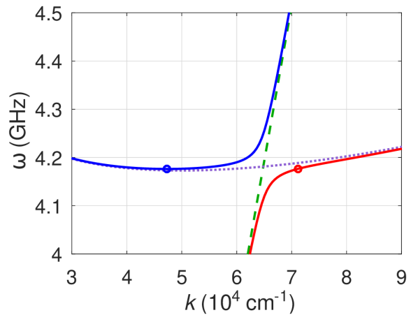
Figure 3: Dispersions of magnetoelastic modes in YIG for momenta parallel to the magnetic field: the blue solid curve represents the $+$ branch while the red solid curve represents the $-$ branch. The blue circle shows the minimum of the dispersion of the $+$ branch and the red circle marks the point where the dispersion of the $-$ branch has the same value. The magnon and phonon dispersions in absence of hybridization are also shown as dotted purple and dashed green line respectively. The film thickness is chosen as $d=6.7\,\mu{\rm m}$ and the magnetic field strength is $H=145\,{\rm mT}.$

The diagonalized quadratic Hamiltonian of the coupled magnon-phonon system then takes the simple form

$${\cal H}^{(2)}= \sum_{\bm{k}}\Bigl{[}E_{{\bm{k}}+}\psi_{{\bm{k}}+}^{\dagger}\psi_{{\bm{k}}+}+E_{{\bm{k}}-}\psi_{{\bm{k}}-}^{\dagger}\psi_{{\bm{k}}-}$$

$$\phantom{\sum_{\bm{k}}}+\omega_{{\bm{k}}\bot}\psi_{{\bm{k}}p}^{\dagger}\psi_{{\bm{k}}p}\Bigr{]}.$$ (14)

The purely phononic operators $\psi_{{\bm{k}}p}$ will not play a role in the following and are hence discarded. Expressing the quartic magnon-magnon interaction (6) in terms of the creation and annihilation operators $\psi_{{\bm{k}}\pm}^{\dagger}$ and $\psi_{{\bm{k}}\pm}$ of the magnetoelastic bosons and dropping some subleading intermodal terms (see below), we obtain

$$\mathcal{H}_{m}^{(4)}\approx \frac{1}{N}\sum_{{\bm{k}}_{1}\dots\bm{k}_{4}}\delta_{{\bm{k}}_{1}+\dots+{\bm{k}}_{4},0}\frac{1}{4}$$

$$\times\Bigl{[}U_{1,2;3,4}^{++++}\psi^{\dagger}_{-1+}\psi^{\dagger}_{-2+}\psi_{3+}\psi_{4+}$$

$$\phantom{\times}+U_{1,2;3,4}^{----}\psi^{\dagger}_{-1-}\psi^{\dagger}_{-2-}\psi_{3-}\psi_{4-}$$

$$\phantom{\times}+U_{1,2;3,4}^{++--}\psi^{\dagger}_{-1+}\psi^{\dagger}_{-2+}\psi_{3-}\psi_{4-}$$

$$\phantom{\times}+U_{1,2;3,4}^{--++}\psi^{\dagger}_{-1-}\psi^{\dagger}_{-2-}\psi_{3+}\psi_{4+}\Bigr{]},$$ (15)

where the subscripts $1,2,\ldots$ represent ${\bm{k}}_{1},{\bm{k}}_{2},\ldots$. The interaction vertices are

$$U_{1,2;3,4}^{\pm\pm\pm\pm}= \left(\phi_{-1\pm}^{1}\right)^{*}\left(\phi_{-2\pm}^{1}\right)^{*}\phi_{3\pm}^{1}\phi_{4\pm}^{1}U_{1,2;3,4},$$ (16a)

$$U_{1,2;3,4}^{\pm\pm\mp\mp}= \left(\phi_{-1\pm}^{1}\right)^{*}\left(\phi_{-2\pm}^{1}\right)^{*}\phi_{3\mp}^{1}\phi_{4\mp}^{1}U_{1,2;3,4},$$ (16b)

and $\phi_{{\bm{k}}\pm}^{1}=(1,0,0)\cdot\bm{\phi}_{{\bm{k}}\pm}$ are the magnonic components of the magnetoelastic wave functions defined in Eq. (12a). The vertices $U_{1,2;3,4}^{\pm\pm\pm\pm}$ describe $++\Leftrightarrow++$ and $--\Leftrightarrow--$ intramodal scattering events where the number of each magnetoelastic boson is conserved. They are responsible for the rapid thermalization of the pumped magnon gas away from the hybridization area. The other class of vertices $U_{1,2;3,4}^{\pm\pm\mp\mp}$ describe $++\Leftrightarrow--$ intermodal scattering events where the number of magnetoelastic bosons in the $+$ or $-$ branch changes by two while the total number of magnetoelastic bosons is conserved. Consequently, these processes exchange both energy and particles between the two magnetoelastic modes and thus are important for the thermalization of the low- and high-energy parts of the magnon spectrum. Because of their energy and momentum conservation constraints, they furthermore lead to a direct coupling of the region around the bottom of the magnon dispersion on the $+$ mode and the nearly degenerate hybridization area of the $-$ mode. Hence, we expect these intermodal processes to be crucial for the eventual appearance of a magnetoelastic accumulation.

Note that in Eq. (15) we have followed the ansatz described in Ref. [Bozhko17, ] and dropped two types of subleading intermodal scattering processes: A $+-\Leftrightarrow+-$ process which does not change the number of bosons in both branches, as well as $++\Leftrightarrow+-$ and $--\Leftrightarrow-+$ processes where the number of bosons on each branch changes only by one. While these scattering processes give rise to additional thermalization channels, we do not expect them to substantially affect the steady state. The first process only redistributes the bosons within the two branches, similar to the intramodal scattering. On the other hand, the second process can lead to an exchange of bosons between the bottom of the $+$ mode and the energetically degenerate hybridization area of the $-$ mode. However, to satisfy energy and momentum conservation, such a scattering requires the participation of high-energy magnons from the $-$ branch. Close to the steady state, we generally expect such processes that also involve high-energy bosons to be less important than the direct scattering between the low-energy bosons and the macroscopically occupied condensate.

III Accumulation of magnetoelastic bosons

In order to describe the experimentally observed accumulation of magnetoelastic bosons, Bozhko17 ; Frey21 we derive in this section quantum kinetic equations for the single-particle distribution functions and the condensation amplitudes of the magnetoelastic modes associated with the bosonic operators $\psi_{{\bm{k}}\pm}$. The kinetic equations are then solved self-consistently to obtain a non-equilibrium steady state which can be compared with experiments.

III.1 Quantum kinetic equations

The dynamics of the connected single-particle distribution function of the magnetoelastic modes,

$$n_{{\bm{k}}\pm}\equiv\langle\psi_{{\bm{k}}\pm}^{\dagger}\psi_{{\bm{k}}\pm}\rangle^{c}\equiv\langle\psi_{{\bm{k}}\pm}^{\dagger}\psi_{{\bm{k}}\pm}\rangle-\left|\Psi_{{\bm{k}}\pm}\right|^{2},$$ (17)

and the dynamics of the associated condensate amplitude (vacuum expectation value)

$$\Psi_{{\bm{k}}\pm}\equiv\langle\psi_{{\bm{k}}\pm}\rangle$$ (18)

can be obtained from the Heisenberg equations of motion of the Bose operators $\psi_{{\bm{k}}\pm}$. We write the equation of motion for the single-particle distribution function in the form

$$\partial_{t}n_{{\bm{k}}\pm}=I_{{\bm{k}}\pm},$$ (19)

where $I_{{\bm{k}}\pm}$ is the relevant collision integral. The derivation of this collision integral is outlined in Appendix C and the approximate expression sufficient for our purpose is given below in Eq. (21). The equation of motion for the condensate amplitude is

$$\partial_{t}\Psi_{{\bm{k}}\pm}+i\left(E_{{\bm{k}}\pm}-\mu_{c}\right)\Psi_{{\bm{k}}\pm}+\frac{i}{2N}\sum_{123}\delta_{1+2+3,\bm{k}}\left[U_{-\bm{k},1;2,3}^{++++}\Psi_{-1+}^{*}\Psi_{2+}\Psi_{3+}+U_{-\bm{k},1;2,3}^{++--}\Psi_{-1+}^{*}\Psi_{2-}\Psi_{3-}\right]=\tilde{I}_{{\bm{k}}\pm},$$ (20)

where $\mu_{c}$ is the chemical potential of the condensate and the collision integral $\tilde{I}_{{\bm{k}}\pm}$ describes scattering into and out of the condensate. The approximate expression for this collision integral that we use is given in Eq. (22) below; for more details we refer to Appendix C. For a realistic description of the experimental setup, this chemical potential $\mu_{c}$ of the condensate is necessary to take into account the approximate number conservation of the magnon subsystem. Physically, the finite value of $\mu_{c}$ is generated by the external pumping and is one of the parameters which characterize the non-equilibrium steady state. The collision integrals $I_{{\bm{k}}\pm}$ and $\tilde{I}_{{\bm{k}}\pm}$ on the right-hand sides of the equations of motion (19) and (20) describe the effect of the quartic interaction (15) on the dynamics; in general, $I_{{\bm{k}}\pm}$ and $\tilde{I}_{{\bm{k}}\pm}$ are complicated functionals of higher-order connected correlation functions, which satisfy additional equations of motion involving even higher-order correlation functions. One of the central problems in quantum kinetic theory is to find a good truncation strategy of this infinite hierarchy of equations of motion. Here we us the method of expansion in connected equal-time correlations developed in Ref. [Fricke97, ] which two of us have recently used Hahn21 to develop a microscopic description of the effect of magnon decays on parametric pumping of magnons in YIG. An advantage of this method is that it directly produces equal-time correlations and that it offers a systematic truncation strategy in powers of connected correlations. The dominant contributions to the collision integrals $I_{{\bm{k}}\pm}$ and $\tilde{I}_{{\bm{k}}\pm}$ in Eqs. (19) and (20) are given in Appendix C, where we also give a diagrammatic representation of the various terms contributing to $I_{{\bm{k}}\pm}$ and $\tilde{I}_{{\bm{k}}\pm}$. Because the magnon-magnon interaction (15) in YIG is suppressed by the small factor of $1/S$, for our purpose it is sufficient to truncate the hierarchy of equations of motion at second order in the interaction. This yields the following expressions for the collision integrals on the right-hand sides of the equations of motion (19) and (20):

$$I_{{\bm{k}}\pm}= \frac{\pi}{4N^{2}}\sum_{123}\delta_{{\bm{k}}+1,2+3}\sum_{r=\pm}\left|U_{-{\bm{k}},-1;2,3}^{\pm\pm rr}\right|^{2}$$

$$\times\Bigl{\{}\delta\left(E_{{\bm{k}}\pm}+E_{1\pm}-E_{2r}-E_{3r}\right)\bigl{[}\left(1+n_{{\bm{k}}\pm}\right)\left(1+n_{1\pm}\right)n_{2r}n_{3r}-n_{{\bm{k}}\pm}n_{1\pm}\left(1+n_{2r}\right)\left(1+n_{3r}\right)\bigr{]}$$

$$\phantom{\times a}-\frac{1}{2}\delta\left(E_{{\bm{k}}\pm}+\mu_{c}-E_{2r}-E_{3r}\right)\left|\Psi_{1\pm}\right|^{2}\bigl{[}\left(1+n_{{\bm{k}}\pm}\right)n_{2r}n_{3r}-n_{{\bm{k}}\pm}\left(1+n_{2r}\right)\left(1+n_{3r}\right)\bigr{]}$$

$$\phantom{\times a}+\delta\left(E_{{\bm{k}}\pm}+E_{1\pm}-E_{2r}-\mu_{c}\right)\left|\Psi_{3r}\right|^{2}\bigl{[}\left(1+n_{{\bm{k}}\pm}\right)\left(1+n_{1\pm}\right)n_{2r}-n_{{\bm{k}}\pm}n_{1\pm}\left(1+n_{2r}\right)\bigr{]}\Bigr{\}},$$ (21)

$$\tilde{I}_{{\bm{k}}\pm}= \frac{\pi}{8N^{2}}\Psi_{{\bm{k}}\pm}\sum_{123}\delta_{{\bm{k}}+1,2+3}\sum_{r=\pm}\left|U_{-{\bm{k}},-1;2,3}^{\pm\pm rr}\right|^{2}$$

$$\times\delta\left(E_{1\pm}+\mu_{c}-E_{2r}-E_{3r}\right)\bigl{[}n_{1\pm}\left(1+n_{2r}\right)\left(1+n_{3r}\right)-\left(1+n_{1\pm}\right)n_{2r}n_{3r}\bigr{]}.$$ (22)

Note that apart from the additional $\pm$ mode label, the resulting kinetic equations coincide with the standard Boltzmann equations for Bose gases known from the literature Zaremba99 .

III.2 Non-equilibrium steady state

In principle, it would be desirable to directly simulate the temporal evolution of the distribution functions and condensate amplitudes that is generated by the coupled integro-differential equations (19) and (20) with the collision integrals given by Eqs. (21) and (22). However, this is a computationally very demanding task because it requires us to cover a large region of momentum space up to comparatively large energies so that thermalization can occur, while at the same time a very fine momentum resolution is necessary to resolve the bottom of the magnon spectrum as well as the energetically degenerate hybridization area in sufficient detail. To circumvent these computational difficulties, we focus on the steady state that eventually forms in the parametrically pumped magnon gas. Then we can take advantage of the fact that the magnon-magnon interaction (6) efficiently thermalizes the magnon gas to a quasi-equilibrium steady state characterized by a finite chemical potential $\mu_{m}$. When this chemical potential approaches the minimum of the magnon dispersion, a condensate is formed.Demokritov06 ; Demidov07 ; Dzyapko07 ; Demidov08a ; Demokritov08 ; Demidov08b ; Serga14 ; Clausen15a ; Clausen15b If the pumping is turned off, the chemical potential and the condensate slowly decay on time scales governed by the weak magnon-phonon interactions.Demokritov06 ; Clausen15a ; Clausen15b As the magnon-phonon hybridization which we aim to include only affects the mode dispersions and interaction amplitudes in a tiny region of momentum space, we may assume that the magnon gas is thermalized almost everywhere in momentum space. In this case the distribution functions of the magnetoelastic modes are described by the incoherent superposition

$$n_{{\bm{k}}\pm}=\left|\phi_{{\bm{k}}\pm}^{1}\right|^{2}n_{{\bm{k}}m}+\left(1-\left|\phi_{{\bm{k}}\pm}^{1}\right|^{2}\right)n_{{\bm{k}}p}$$ (23)

of the thermalized magnon and phonon distributions

$$n_{{\bm{k}}m}= \frac{1}{e^{\left(\epsilon_{{\bm{k}}}-\mu_{m}\right)/T_{m}}-1},$$ (24a)

$$n_{{\bm{k}}p}= \frac{1}{e^{\omega_{{\bm{k}}\bot}/T}-1}.$$ (24b)

Here we take into account that the magnon temperature $T_{m}$ in the steady state can deviate from the temperature $T$ of the phonons. Since these distribution functions annihilate the collision integrals (21) and (22) almost everywhere in momentum space, we can now focus on the small region in momentum space where deviations from Eqs. (23) are expected to occur: The hybridization area where magnons and phonons mix, and the bottom of the magnon spectrum that is energetically degenerate with the hybridization, see Fig. 3. The problem is then reduced to the calculation of the change in the distribution functions and the condensate amplitudes of the two magnetoelastic modes in these two regions. To this end, we develop a self-consistent solution of the kinetic equations (19) and (20) as follows: in a non-equilibrium steady state, the distribution functions and the condensate amplitudes are stationary, so that

$$\partial_{t}n_{{\bm{k}}\pm}= 0,$$ (25a)

$$\partial_{t}\Psi_{{\bm{k}}\pm}= 0.$$ (25b)

Starting from an initial guess for $n_{{\bm{k}}\pm}$ and $\Psi_{{\bm{k}}\pm}$, we can then use the equations of motion (19) and (20) to determine new values for the distribution functions $n_{{\bm{k}}\pm}$ as well as the condensate amplitudes $\Psi_{{\bm{k}}\pm}$. These are in turn used to determine the new values of the collision integrals (21) and (22). This procedure is iterated until convergence is achieved. As initial conditions for the self-consistency loop, we choose the incoherent superposition (23) for $n_{{\bm{k}}\pm}$, whereas the initial condensate density is estimated as follows. We neglect the collision integral in the equation of motion of the condensate amplitude (20) and set the loop momenta in the Gross-Pitaevskii terms equal the external momenta. Demanding that the time derivative of the condensate amplitude vanishes, we then obtain

$$\left|\Psi_{{\bm{k}}r}\right|=\delta_{{\bm{k}},{\bm{k}}_{\rm min}}\delta_{r,+}\sqrt{N\left|\frac{\mu_{c}-E_{{\bm{k}}+}}{U_{-{\bm{k}},-{\bm{k}};{\bm{k}},{\bm{k}}}^{++++}}\right|}.$$ (26)

Here, ${\bm{k}}_{\rm min}$ denotes the wave vector of the minimum of the magnon dispersion that is located in the $+$ branch of the magnetoelastic spectrum. Furthermore, changes in the distribution of the thermal magnon cloud are accounted for by also determining the magnon chemical potential $\mu_{m}$ and temperature $T_{m}$ self-consistently at each iteration. The phonon temperature $T$ on the other hand is kept fixed, reflecting the fact that the phonons act as a thermal bath for the magnons.

For the explicit numerical solution, we parametrize the wave vectors ${\bm{k}}$ by choosing $N_{\theta}$ angles $\theta_{\bm{k}}\in[0,\pi/2]$ and $N_{k}$ points for different lengths $k=|{\bm{k}}|$ of the wave vectors. For each angle $\theta_{\bm{k}}$, the $k$-values are chosen such that they are centered around the minimum of the magnon dispersion for the upper ($+$) mode and the hybridization area for the lower ($-$) mode, see Fig. 3. The resulting non-uniform mesh in momentum space is illustrated in Fig. 4. All modes outside this mesh are modeled with the quasi-equilibrium distribution (23).

(a)

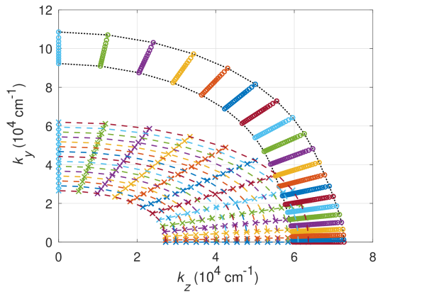
(b)

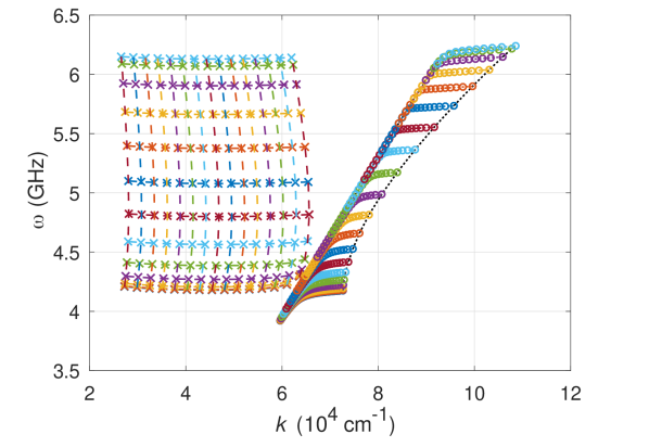
Figure 4: The mesh of wave vectors ${\bm{k}}=\bm{e}_{z}k_{z}+\bm{e}_{y}k_{y}$ consisting of $790$ grid points used for the numerical solution of the kinetic equations in this section. Crosses denote grid points for the upper ($+$) branch and circles denote grid points for the lower ($-$) branch. The upper figure (a) shows the grid in momentum space while the lower figure (b) shows the grid on the plane spanned by $k=|{\bm{k}}|$ and the excitation frequency $\omega$ using the same color coding and symbols as in (a).

To reproduce the experimental situation, the phonon temperature is fixed at room temperature, $T=290\,{\rm K}$, while the external magnetic field and the thickness of the YIG film are set to $H=145\,{\rm mT}$ and $d=6.7\,\mu{\rm m}$ respectively. The condensate chemical potential is set to $\mu_{c}=0.995\,\epsilon_{{\bm{k}}_{\rm min}}$ while we use $T_{m}=T$ and $\mu_{m}=0.98\,\epsilon_{{\bm{k}}_{\rm min}}$ as initial conditions for the self-consistency loop of the temperature and chemical potential of the thermal magnons footnote_muc . The system size appearing in the initial value (26) for the condensate amplitude is set to $N=8.0802\times 10^{6}$.

Our numerical results for the self-consistent steady state are shown in Fig. 5, where the total magnon density

$$\rho_{{\bm{k}}m}=\langle b^{\dagger}_{\bm{k}}b_{\bm{k}}\rangle=\sum_{r=\pm}\left|\phi^{1}_{{\bm{k}}r}\right|^{2}\left(n_{{\bm{k}}r}+\left|\Psi_{{\bm{k}}r}\right|^{2}\right)$$ (27)

is plotted as function of the wave vector ${\bm{k}}=\bm{e}_{z}k_{z}$ parallel to the external field and the excitation frequency $\omega$.

(a)

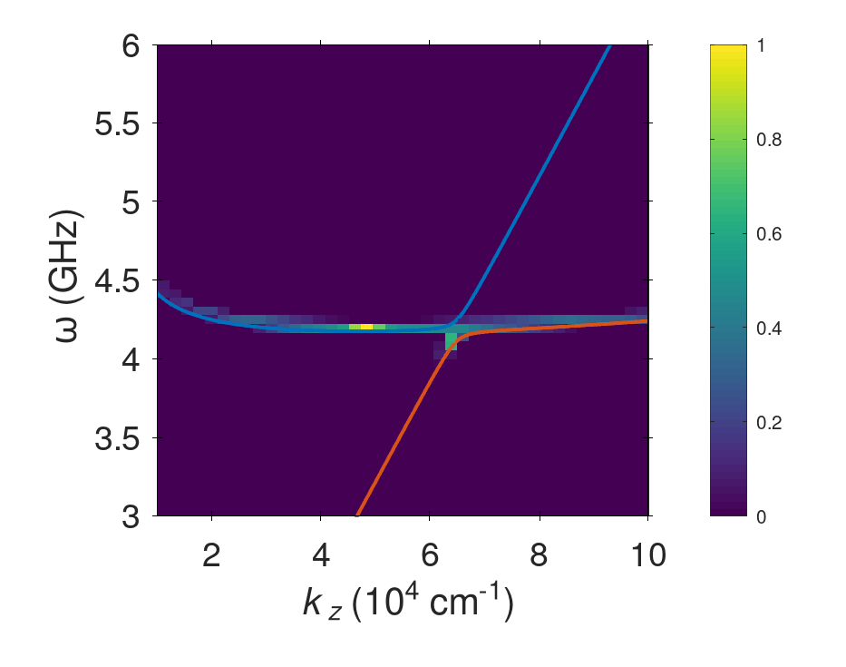
(b)

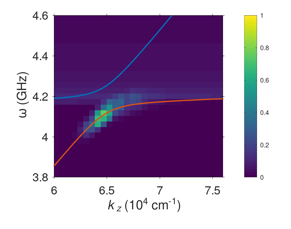
Figure 5: Magnon density $\rho_{{\bm{k}}m}$ as function of the wave vector ${\bm{k}}=\bm{e}_{z}k_{z}$ parallel to the external field and the excitation frequency $\omega$, normalized to the value of the magnon condensate. The dispersion relations of the upper ($+$) and lower ($-$) magnetoelastic modes for wave vectors parallel to the external magnetic field are indicated as blue and red lines respectively. The left peak in (a) is due to the magnon condensate. (b) shows a close-up of the hybridization area.

Apart from the condensate peak at the bottom of the magnon spectrum, one clearly sees the emergence of a second sharp peak in the lower magnetoelastic mode which is located slightly below the bottom of the magnon spectrum in the hybridization area. Despite the narrowness of this peak, our simulations furthermore reveal that it is completely incoherent; i.e., it is not associated with a finite condensate amplitude $\Psi_{{\bm{k}}-}$, but only with the incoherent distribution $n_{{\bm{k}}-}$ of the magnetoelastic bosons. This peak arises due to a bottleneck effect in the intermodal scattering across the hybridization gap, as discussed by Bozhko et al. Bozhko17 .

The change in the magnon density in momentum space is displayed in Fig. 6, which demonstrates that there is no significant deviation from the quasi-equilibrium state away from the bottom of the magnon spectrum for wave vectors parallel to the external magnetic field.

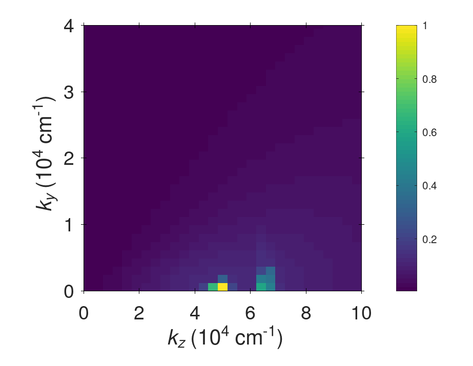
Figure 6: Magnon density $\rho_{{\bm{k}}m}$ in momentum space, normalized as in Fig. 5.

In particular, this means that the hybridization of magnons and phonons, which is a continuous function of the angle $\theta_{\bm{k}}$ between the wave vector and the external magnetic field, is on its own not sufficient to observe an accumulation of magnetoelastic bosons. Instead, the near-degeneracy of this hybridization with the bottom of the magnon spectrum, where the magnon condensate is located, is also necessary. Let us also point out that the temperature and chemical potential of the thermal magnon cloud in this steady state are given by $T_{m}=289.6\,{\rm K}$ and $\mu_{m}=0.978\,\epsilon_{{\bm{k}}_{\rm min}}$ respectively, which is very close to the initial values. Therefore the magnon distribution is virtually unaffected by the hybridization, indicating the adequacy of our quasi-equilibrium ansatz (23) for the incoherent distribution functions away from the hybridization area.

(a)

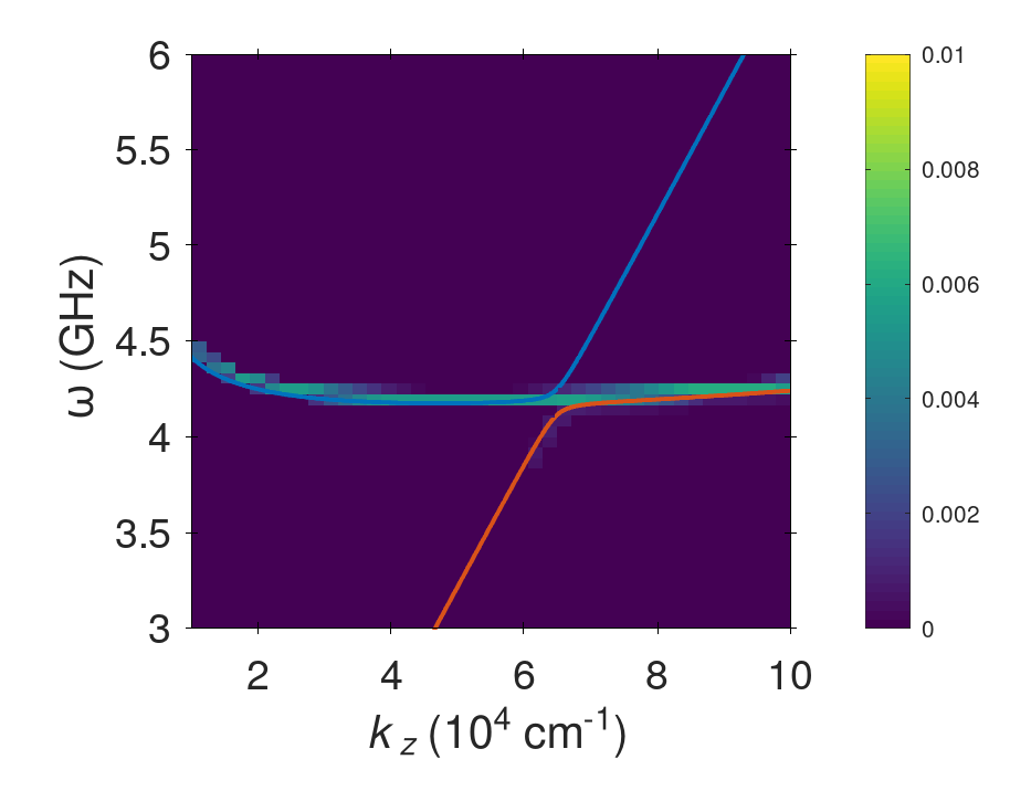
(b)

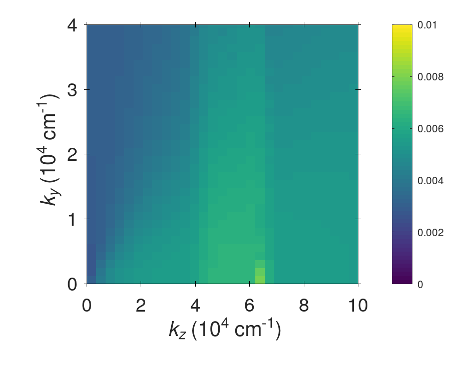
Figure 7: agnon density $\rho_{{\bm{k}}m}$ for a magnon gas that is not sufficiently pumped to establish a magnon condensate, on the same scale as Fig. 5. (a) Magnon density as function of the wave vector ${\bm{k}}=\bm{e}_{z}k_{z}$ parallel to the external field and the excitation frequency $\omega$. The dispersion relations of the upper ($+$) and lower ($-$) magnetoelastic modes for wave vectors parallel to the external magnetic field are indicated as blue and red lines, respectively. (b) Magnon density in momentum space.

To investigate the importance of the magnon condensate for the magnetoelastic accumulation, we also show in Fig. 7 numerical results for the case that the magnon gas is not driven sufficiently strong to form a magnon condensate, with $\mu_{m}=0.75\,\epsilon_{{\bm{k}}_{\rm min}}$. Even in this case, we observe a small bottleneck accumulation in the lower magnetoelastic mode, barely visible in Fig. 7(b). This is in agreement with Ref. [Bozhko17, ], where a magnetoelastic accumulation below the threshold of magnon condensation was reported. However, note the difference in scale: While the magnetoelastic peak in Fig. 5 is of the same order of magnitude as the magnon condensate and hence macroscopic, it is only slightly enhanced compared to the thermal magnon gas without a magnon condensate. Thus, we conclude that the scattering of incoherent magnetoelastic bosons with the nearly degenerate condensate amplitude is an important ingredient for the formation of a macroscopic magnetoelastic peak.

III.3 Comparison with experiment

To further test the predictions of our simulations against experimental observations, we have performed time- and wave vector-resolved Brillouin light scattering (BLS) spectroscopy Sandweg10 measurements of the magnetoelastic accumulation at room temperature in a $d=6.7\,\mu{\rm m}$ thick YIG film with dielectric coating. An external magnetic field $\bm{H}=H{\bm{e}}_{z}$ of 145 mT is applied in-plane parallel to the $z$-axis. Magnons are excited via a parallel parametric pumping Gurevich96 ; Serga12 pulse of length $1500\,{\rm ns}$. During this process photons of the applied microwave field with frequency $f_{p}=14\,{\rm GHz}$ are splitting into two magnons with frequency $f_{p}/2$ and opposite wave vectors. After the pumping pulse is switched off, the magnon gas rapidly thermalizes via number-conserving magnon-magnon scattering processes, generating a finite chemical potential and eventually a magnon condensate at the bottom of the spectrum.

Regarding the BLS spectroscopy experiment, a probing laser beam is focused onto the YIG film and the frequency shift of the scattered light is analyzed with a tandem Fabry-Pérot interferometer. This method is selective for magnons with a certain wave vector depending on the incident angle of the probing laser. Since the BLS setup is only sensitive to modes with a uniform profile along the film normal Bozhko20b , we are only able to detect the magnon intensity in the lowest mode. The BLS intensity depending on the magnon wave vector and energy is shown in Fig. 8.

(a)

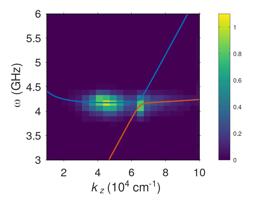
(b)

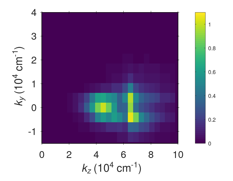
Figure 8: (a) Experimental magnon-phonon spectra and the population of the lowest magnon mode, with the dispersion relations of the upper ($+$) and lower ($-$) magnetoelastic modes for wave vectors parallel to the external magnetic field indicated as blue and red lines, respectively. (b) Wave vector-resolved magnon population. Both plots are normalized to the value of the magnon condensate to facilitate direct comparison with the theoretical prediction in Fig. 5.

Note that these measurements are in good agreement with the numerical results obtained from the solution of the kinetic equations shown in Figs. 5 and 6. In particular, the position of the peak in the magnetoelastic mode agrees very well with our theoretical predictions, while its magnitude is of the same order as the magnon condensate. The overall broader shape of the experimental distributions can at least partially be attributed to a lower resolution than in the numerical simulation. As all qualitative features of the experiment are furthermore reproduced by our calculations, we conclude that our non-equilibrium steady state solution of the kinetic equations correctly describes the relevant physics of the observed magnetoelastic accumulation in YIG.

IV Summary and conclusions

In this work we have studied the accumulation of magnetoelastic bosons – hybrid quasiparticles formed by the coupling of magnons and phonons – in an overpopulated magnon gas in YIG. Starting from an effective spin Hamiltonian and a phenomenological expression for the magnetoelastic energy, we have derived quantum kinetic equations describing the dominant scattering mechanisms for the magnetoelastic bosons, both for the incoherent quasiparticle distribution functions and for the condensate amplitudes. Guided by the observation that the bulk of the magnon and phonon clouds efficiently thermalize to their respective (quasi-)equilibria, we have developed an efficient numerical strategy which has enabled us to self-consistently determine the non-equilibrium steady state from the explicit solution of our kinetic equations without further approximation. This self-consistent steady state solution has allowed us to reproduce the spontaneous accumulation of magnetoelastic bosons in a microscopic calculation. For the first time, we also presented a two-dimensional wave-vector resolved measurement of this accumulation in YIG, which agrees well with our theoretical predictions. In particular, our microscopic theoretical approach based on the self-consistent solution of a quantum kinetic equation quantitatively describes the accumulation of quasiparticles in the hybridization area of the lower magnetoelastic branch, slightly below the bottom of the magnon spectrum.

Our study furthermore clarifies the importance of the magnon condensate for the accumulation of the magnetoelastic bosons: it turns out that the existence of a magnon condensate strongly enhances the accumulation of magnetoelastic bosons. Importantly, we have also shown that despite the spectral narrowness of the accumulation, it resides solely in the incoherent part of the distribution function and is thus not associated with a coherent state. We expect that these findings will be helpful for future studies of this intriguing phenomenon.

APPENDIX A EFFECTIVE MAGNON HAMILTONIAN FOR YIG

To make this work self-contained, we briefly review in this appendix the derivation of the interaction Hamiltonian (6) describing two-body interactions between magnons in YIG. For a more detailed derivation see, for example, Refs. [Kreisel09, ; Hick10, ; Hahn21, ]. With the help of the Holstein-Primakoff transformation Holstein40 the effective spin-Hamiltonian (1) can be expressed in terms of canonical boson operators $c_{i}$ and $c_{i}^{\dagger}$ as usual. Expanding the resulting effective boson Hamiltonian in powers of $1/S$ we obtain

$$\mathcal{H}_{m}=\mathcal{H}_{m}^{(0)}+\mathcal{H}_{m}^{(2)}+\mathcal{H}_{m}^{(3)}+\mathcal{H}_{m}^{(4)}+\mathcal{O}(S^{-1/2}),$$ (A1)

so that $\mathcal{H}_{m}^{(n)}={\cal O}(S^{2-n/2})$ contains the terms of order $n$ in the $c_{i}$ and $c_{i}^{\dagger}$. Transforming to momentum space,

$$c_{i}=\frac{1}{\sqrt{N}}\sum\limits_{\bm{k}}e^{i{\bm{k}}\cdot\bm{r}_{i}}c_{\bm{k}},$$ (A2)

where $N$ denotes the number of lattice sites in the $yz$-plane, we find that the quadratic part $\mathcal{H}_{m}^{(2)}$ of the Hamiltonian can be written as Hick10

$$\mathcal{H}_{m}^{(2)}=\sum\limits_{\bm{k}}\left[A_{\bm{k}}c^{\dagger}_{\bm{k}}c_{\bm{k}}+\frac{B_{\bm{k}}}{2}\left(c^{\dagger}_{\bm{k}}c^{\dagger}_{-{\bm{k}}}+c_{-{\bm{k}}}c_{\bm{k}}\right)\right],$$ (A3)

where

$$A_{\bm{k}} = h+S\left(J_{\bm{0}}-J_{\bm{k}}\right)+S\left[D^{zz}_{\bm{0}}-\frac{1}{2}\left(D^{xx}_{\bm{k}}+D^{yy}_{\bm{k}}\right)\right],$$

$$B_{\bm{k}} = -\frac{S}{2}\left[D^{xx}_{\bm{k}}-2iD^{xy}_{\bm{k}}-D^{yy}_{\bm{k}}\right],$$ (A5)

and the Fourier transforms of the exchange and dipolar couplings are defined by

$$J_{\bm{k}} = \sum\limits_{i}\text{e}^{-i{\bm{k}}\cdot\bm{r}_{ij}}J_{ij},$$ (A6)

$$D^{\alpha\beta}_{\bm{k}} = \sum\limits_{i}\text{e}^{-i{\bm{k}}\cdot\bm{r}_{ij}}D^{\alpha\beta}_{ij}.$$ (A7)

As explained in Sec. II.1, the cubic part ${\cal{H}}_{n}^{(3)}$ of the Hamiltonian can be neglected for our purpose because energy and momentum conservation cannot be fulfilled by the cubic interactions in the parameter regime of interest to us. Therefore we need only the quartic part of the Hamiltonian, which reads Hick10

$$\mathcal{H}_{m}^{(4)} = \frac{1}{N}\sum\limits_{{\bm{k}}_{1}\dots\bm{k}_{4}}\delta_{{\bm{k}}_{1}+{\bm{k}}_{2}+{\bm{k}}_{3}+{\bm{k}}_{4},0}$$ (A8)

$$\times\Biggl{[}\frac{1}{\left(2!\right)^{2}}\Gamma^{\bar{c}\bar{c}cc}_{1,2;3,4}c^{\dagger}_{-1}c^{\dagger}_{-2}c_{3}c_{4}$$

$$\phantom{\times}+\frac{1}{3!}\Gamma^{\bar{c}ccc}_{1;2,3,4}c^{\dagger}_{-1}c_{2}c_{3}c_{4}$$

$$\phantom{\times}+\frac{1}{3!}\Gamma^{\bar{c}\bar{c}\bar{c}c}_{1,2,3;4}c^{\dagger}_{-1}c^{\dagger}_{-2}c^{\dagger}_{-3}c_{4}\Biggr{]},$$

where we abbreviate the momenta ${\bm{k}}_{i}$ by $i$. The vertices are given by

$$\Gamma^{\bar{c}\bar{c}cc}_{1,2;3,4} = -\frac{1}{2}\Biggl{[}J_{{\bm{k}}_{1}+{\bm{k}}_{3}}+J_{{\bm{k}}_{2}+{\bm{k}}_{3}}+J_{{\bm{k}}_{1}+{\bm{k}}_{4}}+J_{{\bm{k}}_{2}+{\bm{k}}_{4}}$$ (A9a)

$$+D^{zz}_{{\bm{k}}_{1}+{\bm{k}}_{3}}+D^{zz}_{{\bm{k}}_{2}+{\bm{k}}_{3}}+D^{zz}_{{\bm{k}}_{1}+{\bm{k}}_{4}}+D^{zz}_{{\bm{k}}_{2}+{\bm{k}}_{4}}$$

$$-\sum\limits_{i=1}^{4}\left(J_{{\bm{k}}_{i}}-2D^{zz}_{{\bm{k}}_{i}}\right)\Biggr{]},$$

$$\Gamma^{\bar{c}ccc}_{1;2,3,4} = \frac{1}{4}\left[D^{xx}_{{\bm{k}}_{2}}-2iD^{xy}_{{\bm{k}}_{2}}-D^{yy}_{{\bm{k}}_{2}}+D^{xx}_{{\bm{k}}_{3}}-2iD^{xy}_{{\bm{k}}_{3}}-D^{yy}_{{\bm{k}}_{3}}\right.$$ (A9b)

$$\left.+D^{xx}_{{\bm{k}}_{4}}-2iD^{xy}_{{\bm{k}}_{4}}-D^{yy}_{{\bm{k}}_{4}}\right],$$

$$\Gamma^{\bar{c}\bar{c}\bar{c}c}_{1,2,3;4} = \left(\Gamma^{\bar{c}ccc}_{4;1,2,3}\right)^{*}.$$ (A9c)

The quadratic part $\mathcal{H}_{m}^{(2)}$ of the Hamiltonian can be diagonalized by the Bogoliubov transformation to new canonical Bose operators $b_{{\bm{k}}}$ and $b_{{\bm{k}}}^{\dagger}$,

$$\left(\begin{array}[]{c}c_{\bm{k}}\\ c^{\dagger}_{-{\bm{k}}}\end{array}\right)=\left(\begin{array}[]{cc}u_{\bm{k}}&-v_{\bm{k}}\\ -v_{\bf{k}}^{\ast}&u_{\bm{k}}\end{array}\right)\left(\begin{array}[]{c}b_{{\bm{k}}}\\ b^{\dagger}_{-{\bm{k}}}\end{array}\right),$$ (A10)

where the Bogoliubov coefficients are

$$u_{\bm{k}} = \sqrt{\frac{A_{\bm{k}}+\varepsilon_{\bm{k}}}{2\varepsilon_{\bm{k}}}},$$ (A11a)

$$v_{\bm{k}} = \frac{B_{\bm{k}}}{|B_{\bm{k}}|}\sqrt{\frac{A_{\bm{k}}-\varepsilon_{\bm{k}}}{2\varepsilon_{\bm{k}}}},$$ (A11b)

and the magnon dispersion $\epsilon_{\bm{k}}$ is given by

$$\epsilon_{\bm{k}}=\sqrt{A_{\bm{k}}^{2}-|B_{\bm{k}}|^{2}}.$$ (A12)

In terms of the new Bose operators, the quadratic part of the Hamiltonian has the form

$$\mathcal{H}_{m}^{(2)}=\sum\limits_{\bm{k}}\left[\epsilon_{\bm{k}}b^{\dagger}_{\bm{k}}b_{\bm{k}}+\frac{A_{\bm{k}}-\epsilon_{\bm{k}}}{2\epsilon_{\bm{k}}}\right].$$ (A13)

By neglecting the constant term in Eq. (A13) above, we arrive at Eq. (3). Finally, applying the Bogoliubov transformation (A10) to the quartic Hamiltonian (A8) and dropping the terms that do not conserve the magnon number yields the interaction Hamiltonian (6), with the quartic vertex explicitly given by

$$U_{1,2;3,4} = \phantom{..}\Gamma^{\bar{c}\bar{c}cc}_{1,2;3,4}u_{1}u_{2}u_{3}u_{4}+\Gamma^{\bar{c}\bar{c}cc}_{1,3;4,2}u_{1}u_{4}v_{3}v_{2}$$

$$+\Gamma^{\bar{c}\bar{c}cc}_{1,4;3,2}u_{1}u_{3}v_{4}v_{2}+\Gamma^{\bar{c}\bar{c}cc}_{2,3;4,1}u_{2}u_{4}v_{3}v_{1}$$

$$+\Gamma^{\bar{c}\bar{c}cc}_{2,4;3,1}u_{2}u_{3}v_{4}v_{1}+\Gamma^{\bar{c}\bar{c}cc}_{3,4;2,1}v_{1}v_{2}v_{3}v_{4}$$

$$-\Gamma^{\bar{c}ccc}_{4;3,2,1}u_{3}v_{2}v_{1}v_{4}-\Gamma^{\bar{c}ccc}_{3;4,2,1}u_{4}v_{2}v_{1}v_{3}$$

$$-\Gamma^{\bar{c}ccc}_{2;3,4,1}u_{2}u_{3}u_{4}v_{1}-\Gamma^{\bar{c}ccc}_{1;3,4,2}u_{1}u_{3}u_{4}v_{2}$$

$$-\Gamma^{\bar{c}\bar{c}\bar{c}c}_{2,3,4;1}u_{2}v_{3}v_{4}v_{1}-\Gamma^{\bar{c}\bar{c}\bar{c}c}_{1,3,4;2}u_{1}v_{3}v_{4}v_{2}$$

$$-\Gamma^{\bar{c}\bar{c}\bar{c}c}_{1,2,4;3}u_{1}u_{2}u_{3}v_{4}-\Gamma^{\bar{c}\bar{c}\bar{c}c}_{1,2,3;4}u_{1}u_{2}u_{4}v_{3}.$$

APPENDIX B QUANTIZATION OF THE MAGNETOELASTIC ENERGY

In order to quantize the magnetoelastic energy (8), we first note that the (linear) symmetric strain tensor $X^{\alpha\beta}(\bm{r})$ can be expressed in terms of the phonon displacement field $\bm{X}(\bm{r})$ as Landau70

$$X^{\alpha\beta}(\bm{r})=\frac{1}{2}\left[\frac{\partial X^{\alpha}(\bm{r})}{\partial r^{\beta}}+\frac{\partial X^{\beta}(\bm{r})}{\partial r^{\alpha}}\right].$$ (B1)

Following the standard approach of expanding the displacement field in terms of the phonon creation and annihilation operators $a_{{\bm{k}}\lambda}^{\dagger}$ and $a_{{\bm{k}}\lambda}$ then yields

$$\bm{X}(\bm{r})\to\frac{1}{\sqrt{N}}\sum_{{\bm{k}}\lambda}e^{i{\bm{k}}\cdot\bm{r}}\frac{a_{{\bm{k}}\lambda}+a_{-{\bm{k}}\lambda}^{\dagger}}{\sqrt{2\rho n\omega_{{\bm{k}}\lambda}}}\bm{e}_{{\bm{k}}\lambda}\;.$$ (B2)

where $n=1/a^{3}$ is the number density of ions and $\rho\approx 5.17\;\mbox{g}/\mbox{cm}^{2}$ is the mass density of YIG. The phonon polarization vectors $\bm{e}_{{\bm{k}}\lambda}=\bm{e}_{-{\bm{k}}\lambda}^{*}$ satisfy the orthogonality and completeness relations $\bm{e}_{{\bm{k}}\lambda}^{*}\cdot\bm{e}_{{\bm{k}}\lambda^{\prime}}=\delta_{\lambda\lambda^{\prime}}$ and $\sum_{\lambda}\bm{e}_{{\bm{k}}\lambda}\bm{e}_{{\bm{k}}\lambda}^{\dagger}={\bf 1}$. In the thin film geometry of Fig. 1, a convenient choice for the three polarization vectors is Rueckriegel14

$$\bm{e}_{{\bm{k}}\parallel}= i{\bm{k}}/|{\bm{k}}|=i\left(\bm{e}_{z}\cos\theta_{\bm{k}}+\bm{e}_{y}\sin\theta_{\bm{k}}\right),$$ (B3a)

$$\bm{e}_{{\bm{k}}\bot 1}= i\left(\bm{e}_{z}\sin\theta_{\bm{k}}+\bm{e}_{y}\cos\theta_{\bm{k}}\right),$$ (B3b)

$$\bm{e}_{{\bm{k}}\bot 2}= \bm{e}_{x}.$$ (B3c)

To leading order in $1/S$, the local magnetization is quantized by replacing

$$M^{x}(\bm{r})\to \frac{\mu n}{\sqrt{N}}\sum_{{\bm{k}}}e^{i{\bm{k}}\cdot\bm{r}}\sqrt{\frac{S}{2}}\left(c_{\bm{k}}+c_{-{\bm{k}}}^{\dagger}\right),$$ (B4a)

$$M^{y}(\bm{r})\to \frac{\mu n}{\sqrt{N}}\sum_{{\bm{k}}}e^{i{\bm{k}}\cdot\bm{r}}\frac{1}{i}\sqrt{\frac{S}{2}}\left(c_{\bm{k}}-c_{-{\bm{k}}}^{\dagger}\right),$$ (B4b)

$$M^{z}(\bm{r})\to \mu nS.$$ (B4c)

With this prescription the classical magnetoelastic energy $E_{\rm me}$ defined in Eq. (8) is replaced by the quantized magnon-phonon Hamiltonian ${\cal H}_{mp}^{(2)}+{\cal O}(1/S)$ with

$$\mathcal{H}_{mp}^{(2)}=\frac{1}{2}\sum_{{\bm{k}}\lambda}\gamma_{{\bm{k}}\lambda}\left(a_{-{\bm{k}}\lambda}+a_{{\bm{k}}\lambda}^{\dagger}\right)c_{\bm{k}}+{\rm h.c.}\;\;.$$ (B5)

For the thin-film geometry shown in Fig. 1 the hybridization vertices are given by Rueckriegel14

$$\gamma_{{\bm{k}}\parallel}= i\frac{B_{\bot}}{\sqrt{S\rho n\omega_{{\bm{k}}\lambda}}}\frac{2k_{y}k_{z}}{|{\bm{k}}|}=i\frac{B_{\bot}}{\sqrt{S\rho n\omega_{{\bm{k}}\lambda}}}|{\bm{k}}|\sin\left(2\theta_{\bm{k}}\right),$$ (B6a)

$$\gamma_{{\bm{k}}\bot 1}= i\frac{B_{\bot}}{\sqrt{S\rho n\omega_{{\bm{k}}\lambda}}}\frac{k_{y}^{2}-k_{z}^{2}}{|{\bm{k}}|}=-i\frac{B_{\bot}}{\sqrt{S\rho n\omega_{{\bm{k}}\lambda}}}|{\bm{k}}|\cos\left(2\theta_{\bm{k}}\right),$$ (B6b)

$$\gamma_{{\bm{k}}\bot 2}= -i\frac{B_{\bot}}{\sqrt{S\rho n\omega_{{\bm{k}}\lambda}}}k_{z}=-i\frac{B_{\bot}}{\sqrt{S\rho n\omega_{{\bm{k}}\lambda}}}|{\bm{k}}|\cos\theta_{\bm{k}}.$$ (B6c)

In the last step, we apply the Bogoliubov transformation (A10) to the magnon operators, which yields the magnon-phonon hybridization Hamiltonian given in Eq. (9), with the transformed hybridization vertices

$$\Gamma_{{\bm{k}}\lambda}=u_{\bm{k}}\gamma_{{\bm{k}}\lambda}-v_{\bm{k}}^{*}\gamma_{-{\bm{k}}\lambda}^{*}.$$ (B7)

APPENDIX C COLLISION INTEGRALS

In this appendix we outline the derivation of the collision integrals $I_{{\bm{k}}\pm}$ and $\tilde{I}_{{\bm{k}}\pm}$ in Eqs. (21) and (22). Therefore we use the method developed in Ref. [Fricke97, ] which produces a systematic expansion of the collision integrals in powers of connected equal-time correlation functions, see also Ref. [Hahn21, ] for a recent application of this method in the context of YIG.

Let us start with the collision integral $I_{{\bm{k}}\pm}$ which controls the time-derivative $\partial_{t}n_{{\bm{k}}\pm}$ of the distribution of the magnetoelastic modes. A diagrammatic representation of the various terms contributing to this collision integral is shown in Fig. 9. Note that the circles in Fig. 9 represent the exact equal-time correlations, while the black dots represent the bare four-point vertices defined in Eq. (16).

Figure 9: The diagrams contributing to the time evolution of the correlation $n_{{\bm{k}}+}=\langle\psi_{{\bm{k}}+}^{\dagger}\psi_{{\bm{k}}+}\rangle^{c}$ in an approximation where only the quartic vertices are retained. Note that the diagrams used here differ from Feynman diagrams as they represent contributions to the differential equations for the correlations at a fixed time. External vertices denote creation operators (outgoing arrows) or annihilation operators (incoming arrows) and internal vertices denote the bare interactions. Lines between the interaction vertices and external vertices represent connected correlations of order two where solid lines denote the upper ($+$) branch and dashed lines denote the lower ($-$) branch. The circles represent connected correlations.

Figure 10: The diagrams contributing to the time evolution of the correlations $\langle\psi_{{\bm{k}}_{1}+}^{\dagger}\psi_{{\bm{k}}_{2}+}^{\dagger}\psi_{{\bm{k}}_{3}+}\psi_{{\bm{k}}_{4}+}\rangle^{c}$ (left) and $\langle\psi_{{\bm{k}}_{1}+}^{\dagger}\psi_{{\bm{k}}_{2}+}^{\dagger}\psi_{{\bm{k}}_{3}-}\psi_{{\bm{k}}_{4}-}\rangle^{c}$ (right). The diagrams contain only the intramodal scattering vertex $U_{1,2;3,4}^{++++}$ and the intermodal scattering vertex $U_{1,2;3,4}^{++--}$. Diagrams containing correlations are of higher order in the interaction vertices and are neglected here.

Figure 11: The diagrams contributing to the time evolution of the condensate amplitude $\Psi_{{\bm{k}}+}=\langle\psi_{{\bm{k}}+}\rangle$. The graphical elements are defined in the caption of Fig. 9. The two diagrams in the second line represent the Gross-Pitaevskii term on the left-hand side of the equation of motion (20) for the condensate density $\Psi_{\bm{k}\pm}$.

Figure 12: The diagrams contributing to the time evolution of the three-field correlations $\langle\psi_{{\bm{k}}_{1}+}\psi_{{\bm{k}}_{2}+}^{\dagger}\psi_{{\bm{k}}_{3}+}^{\dagger}\rangle^{c}$ (left) and $\langle\psi_{{\bm{k}}_{1}+}\psi_{{\bm{k}}_{2}-}^{\dagger}\psi_{{\bm{k}}_{3}-}^{\dagger}\rangle^{c}$ (right) contain the condensate amplitude and the intramodal scattering vertex $U_{1,2;3,4}^{++++}$ (left) and the intermodal scattering vertex $U_{1,2;3,4}^{++--}$ (right). The symbols have the same meaning as in Fig. 9. Note that diagrams containing higher order correlations are neglected here because they lead to terms of higher order in the interaction vertices.

These diagrams represent the following mathematical expression,

$$I_{{\bm{k}}+} = \frac{i}{2N}\sum\limits_{{\bm{q}}_{1},{\bm{q}}_{2},{\bm{q}}_{3}}\delta_{{\bm{k}}+{\bm{q}}_{1}-{\bm{q}}_{2}-{\bm{q}}_{3},0}\left[U^{++++}_{-{\bm{k}},-{\bm{q}}_{1};{\bm{q}}_{2},{\bm{q}}_{3}}\langle\psi_{{\bm{q}}_{2}+}^{\dagger}\psi_{{\bm{q}}_{3}+}^{\dagger}\psi_{{\bm{k}}+}\psi_{{\bm{q}}_{1}+}\rangle^{c}+U^{++--}_{-{\bm{k}},-{\bm{q}}_{1};{\bm{q}}_{2},{\bm{q}}_{3}}\langle\psi_{{\bm{q}}_{2}-}^{\dagger}\psi_{{\bm{q}}_{3}-}^{\dagger}\psi_{{\bm{k}}+}\psi_{{\bm{q}}_{1}+}\rangle^{c}-\mathrm{c.c.}\right].$$ (C1)

$$+\frac{i}{2N}\sum\limits_{{\bm{q}}_{1},{\bm{q}}_{2},{\bm{q}}_{3}}\delta_{{\bm{k}}+{\bm{q}}_{1}-{\bm{q}}_{2}-{\bm{q}}_{3},0}\Biggl{[}U^{++++}_{-{\bm{k}},-{\bm{q}}_{1};{\bm{q}}_{2},{\bm{q}}_{3}}\langle\psi_{{\bm{q}}_{2}+}^{\dagger}\psi_{{\bm{q}}_{3}+}^{\dagger}\psi_{{\bm{k}}+}\rangle^{c}\langle\psi_{{\bm{q}}_{1}+}\rangle^{c}+2U^{++++}_{-{\bm{k}},-{\bm{q}}_{1};{\bm{q}}_{2},{\bm{q}}_{3}}\langle\psi_{{\bm{q}}_{1}+}^{\dagger}\psi_{{\bm{q}}_{2}+}\psi_{{\bm{k}}+}\rangle^{c}\langle\psi_{{\bm{q}}_{3}+}^{\dagger}\rangle^{c}$$

$$+U^{++--}_{-{\bm{k}},-{\bm{q}}_{1};{\bm{q}}_{2},{\bm{q}}_{3}}\langle\psi_{{\bm{q}}_{2}-}^{\dagger}\psi_{{\bm{q}}_{3}-}^{\dagger}\psi_{{\bm{k}}+}\rangle^{c}\langle\psi_{{\bm{q}}_{1}+}\rangle^{c}+2U^{++--}_{-{\bm{k}},-{\bm{q}}_{1};{\bm{q}}_{2},{\bm{q}}_{3}}\langle\psi_{{\bm{q}}_{1}+}^{\dagger}\psi_{{\bm{q}}_{2}-}\psi_{{\bm{k}}+}\rangle^{c}\langle\psi_{{\bm{q}}_{3}-}^{\dagger}\rangle^{c}-\mathrm{c.c.}\Biggr{]}.$$

For the four-point and three-point correlations in this expression, we use again their equations of motion. We will explicitly show only the calculations for the term shown in Fig. 9 contributing to the equation of motion of $\langle\psi_{{\bm{q}}_{2}+}^{\dagger}\psi_{{\bm{q}}_{3}+}^{\dagger}\psi_{{\bm{k}}+}\psi_{{\bm{q}}_{1}+}\rangle^{c}$ as an example which is,

$$\left[\frac{d}{dt}+i\left(E_{{\bm{k}}+}+E_{{\bm{q}}_{1}+}-E_{{\bm{q}}_{2}+}-E_{{\bm{q}}_{3}+}\right)\right]\langle\psi_{{\bm{q}}_{2}+}^{\dagger}\psi_{{\bm{q}}_{3}+}^{\dagger}\psi_{{\bm{k}}+}\psi_{{\bm{q}}_{1}+}\rangle^{c}$$ (C2)

$$= \frac{i}{4N}U^{++++}_{-{\bm{q}}_{2},-{\bm{q}}_{3};{\bm{k}},{\bm{q}}_{1}}\biggl{(}\langle\psi_{{\bm{k}}+}\psi_{{\bm{k}}+}^{\dagger}\rangle^{c}\langle\psi_{{\bm{q}}_{1}+}\psi_{{\bm{q}}_{1}+}^{\dagger}\rangle^{c}\langle\psi_{{\bm{q}}_{2}+}^{\dagger}\psi_{{\bm{q}}_{2}+}\rangle^{c}\langle\psi_{{\bm{q}}_{3}+}^{\dagger}\psi_{{\bm{q}}_{3}+}\rangle^{c}$$

$$\hskip 80.0pt-\langle\psi_{{\bm{k}}+}^{\dagger}\psi_{{\bm{k}}+}\rangle^{c}\langle\psi_{{\bm{q}}_{1}+}^{\dagger}\psi_{{\bm{q}}_{1}+}\rangle^{c}\langle\psi_{{\bm{q}}_{2}+}\psi_{{\bm{q}}_{2}+}^{\dagger}\rangle^{c}\langle\psi_{{\bm{q}}_{3}+}\psi_{{\bm{q}}_{3}+}^{\dagger}\rangle^{c}\biggr{)}+\dots$$

$$= \frac{i}{4N}U^{++++}_{-{\bm{q}}_{2},-{\bm{q}}_{3};{\bm{k}},{\bm{q}}_{1}}\left[\left(1+n_{{\bm{k}}+}\right)\left(1+n_{1+}\right)n_{2+}n_{3+}-n_{{\bm{k}}+}n_{1+}\left(1+n_{2+}\right)\left(1+n_{3+}\right)\right]+\dots.$$

The other contributions denoted by the dots contain three-point, four-point or six-point correlations, which we neglect to leading order in the interaction. As the contributions from the other diagrams have the same form the calculations are analogous for all terms. We now integrate this equation to obtain the formal result

$$\langle\psi_{{\bm{q}}_{2}+}^{\dagger}\psi_{{\bm{q}}_{3}+}^{\dagger}\psi_{{\bm{k}}+}\psi_{{\bm{q}}_{1}+}\rangle^{c} = \frac{i}{4N}\int\limits_{t_{0}}^{t}dt^{\prime}\cos\left[\left(E_{{\bm{k}}+}+E_{{\bm{q}}_{1}+}-E_{{\bm{q}}_{2}+}-E_{{\bm{q}}_{3}+}\right)\left(t-t^{\prime}\right)\right]U^{++++}_{-{\bm{q}}_{2},-{\bm{q}}_{3};{\bm{k}},{\bm{q}}_{1}}$$ (C3)

$$\times\left[\left(1+n_{{\bm{k}}+}\right)\left(1+n_{1+}\right)n_{2+}n_{3+}-n_{{\bm{k}}+}n_{1+}\left(1+n_{2+}\right)\left(1+n_{3+}\right)\right]+\dots.$$

Inserting Eq. (C3) into Eq. (C1) then leads to

$$I_{{\bm{k}}+}=\frac{1}{4N^{2}}\sum\limits_{{\bm{q}}_{1},{\bm{q}}_{2},{\bm{q}}_{3}}\delta_{{\bm{k}}+{\bm{q}}_{1}-{\bm{q}}_{2}-{\bm{q}}_{3},0}\left|U^{++++}_{-{\bm{k}},-{\bm{q}}_{1};{\bm{q}}_{2},{\bm{q}}_{3}}\right|^{2}\int\limits_{t_{0}}^{t}dt^{\prime}\cos\left[\left(E_{{\bm{k}}+}+E_{{\bm{q}}_{1}+}-E_{{\bm{q}}_{2}+}-E_{{\bm{q}}_{3}+}\right)\left(t-t^{\prime}\right)\right]$$

$$\times\left[\left(1+n_{{\bm{k}}+}\right)\left(1+n_{1+}\right)n_{2+}n_{3+}-n_{{\bm{k}}+}n_{1+}\left(1+n_{2+}\right)\left(1+n_{3+}\right)\right]+\dots.$$ (C4)

$$\underrightarrow{t_{0}\rightarrow-\infty}\;\frac{\pi}{4N^{2}}\sum\limits_{{\bm{q}}_{1},{\bm{q}}_{2},{\bm{q}}_{3}}\delta_{{\bm{k}}+{\bm{q}}_{1}-{\bm{q}}_{2}-{\bm{q}}_{3},0}\left|U^{++++}_{-{\bm{k}},-{\bm{q}}_{1};{\bm{q}}_{2},{\bm{q}}_{3}}\right|^{2}\delta\left(E_{{\bm{k}}+}+E_{{\bm{q}}_{1}+}-E_{{\bm{q}}_{2}+}-E_{{\bm{q}}_{3}+}\right)$$

$$\times\left[\left(1+n_{{\bm{k}}+}\right)\left(1+n_{1+}\right)n_{2+}n_{3+}-n_{{\bm{k}}+}n_{1+}\left(1+n_{2+}\right)\left(1+n_{3+}\right)\right]+\dots,$$ (C5)

where in the last step we have taken the limit $t_{0}\rightarrow-\infty$. In this way all terms entering the equation of motion for the one-particle distribution functions can be expressed in terms of the bare interaction vertices.

Finally, let us also give the diagrams contributing to the collision integral $\tilde{I}_{{\bm{k}}\pm}$ in Eq. (22) which appears in the equation of motion (20) for the condensate density $\Psi_{\bm{k}\pm}$. The diagrams in the first line of Fig. 11 represent the contributions to the equation of motion for the condensate density $\Psi_{\bm{k}\pm}$ involving higher-order correlations. On the other hand, the diagrams in the second line of Fig. 11 correspond to the Gross-Pitaevskii term which is not included in the collision integral in Eq. (20).

To lowest order in the interaction, the equation of motion for the three-point correlations in the diagrams of the first line of Fig. 12 can be expressed again in terms of the bare four-point vertices as shown in Fig. 12.

References

- (1) E. Abrahams and C. Kittel, Spin-Lattice Relaxation in Ferromagnets, Phys. Rev. 88, 1200 (1952); Relaxation Process in Ferromagnetism, Rev. Mod. Phys. 25, 233 (1953).
- (2) D. A. Bozhko, V. I. Vasyuchka, A. V. Chumak, and A. A. Serga, Magnon-phonon interactions in magnon spintronics (Review article), Low Temp. Phys. 46, 383 (2020).
- (3) A. Kamra and G. E. W. Bauer, Actuation, propagation, and detection of transverse magnetoelastic waves in ferromagnets, Solid State Commun. 198, 35 (2014).
- (4) A. Rückriegel, P. Kopietz, D. A. Bozhko, A. A. Serga, and B. Hillebrands, Magnetoelastic modes and lifetime of magnons in thin yttrium iron garnet films, Phys. Rev. B 89, 184413 (2014).
- (5) N. Ogawa, W. Koshibae, A. J. Beekman, N. Nagaosa, M. Kubota, M. Kawasaki, and Y. Tokura, Photodrive of magnetic bubbles via magnetoelastic waves, Proc. Natl. Acad. Sci. USA 112, 8977 (2015).
- (6) T. Kikkawa, K. Shen, B. Flebus, R. A. Duine, K. Uchida, Z. Qiu, G. E. W. Bauer, and E. Saitoh, Magnon polarons in the spin Seebeck effect, Phys. Rev. Lett. 117, 207203 (2016).
- (7) R. Takahashi and N. Nagaosa, Berry Curvature in Magnon-Phonon Hybrid Systems, Phys. Rev. Lett. 117, 217205 (2016).
- (8) V. G. Baryakhtar and A. G. Danilevich, Magnetoelastic oscillations in ferromagnets with cubic symmetry, Low Temp. Phys. 43, 351 (2017).
- (9) R. Ramos, T. Hioki, Y. Hashimoto, T. Kikkawa, P. Frey, A. J. E. Kreil, V. I. Vasyuchka, A. A. Serga, B. Hillebrands, and E. Saitoh, Room temperature and low-field resonant enhancement of spin Seebeck effect in partially compensated magnets Nat. Commun. 10, 5162 (2019).
- (10) A. Rückriegel and R. A. Duine, Long-range phonon spin transport in ferromagnet-nonmagnetic insulator heterostructures, Phys. Rev. Lett. 124, 117201 (2020).
- (11) D. A. Bozhko, P. Clausen, G. A. Melkov, V. S. L’vov, A. Pomyalov, V. I. Vasyuchka, A. V. Chumak, B. Hillebrands, and A. A. Serga, Bottleneck Accumulation of Hybrid Magnetoelastic Bosons, Phys. Rev. Lett. 118, 237201 (2017).
- (12) A. Kreisel, F. Sauli, L. Bartosch, and P. Kopietz, Microscopic spin-wave theory for yttrium-iron garnet films, Eur. Phys. J. B 71, 59 (2009).
- (13) B. A. Kalinikos, and A. N. Slavin, Theory of dipole-exchange spin wave spectrum for ferromagnetic films with mixed exchange boundary conditions, J. Phys. C 19, 7013 (1986).
- (14) P. Frey, D. A. Bozhko, V. S. L’vov, B. Hillebrands, and A. A. Serga, Double accumulation and anisotropic transport of magneto-elastic bosons in yttrium iron garnet films, Phys. Rev. B 104, 014420 (2021).
- (15) J. Fricke, Transport Equations Including Many-Particle Correlations for an Arbitrary Quantum System: A General Formalism, Ann. Phys. 252, 479 (1996); see also J. Fricke, Transportgleichungen für quantenmechanische Vielteilchensystems, (Cuvillier Verlag, Göttingen, 1996).
- (16) V. Hahn and P. Kopietz, Effect of magnon decays on parametrically pumped magnons, Phys. Rev. B 103, 094416 (2021).
- (17) V. Cherepanov, I. Kolokolov, and V. L’vov, The saga of YIG: spectra, thermodynamics, interaction and relaxation of magnons in a complex magnet, Phys. Rep. 229, 81 (1993).
- (18) I. S. Tupitsyn, P. C. E. Stamp, and A. L. Burin, Stability of Bose-Einstein Condensates of Hot Magnons in Yttrium Iron Garnet Films, Phys. Rev. Lett. 100, 257202 (2008).
- (19) T. Holstein and H. Primakoff, Field Dependence of the Intrinsic Domain Magnetization of a Ferromagnet, Phys. Rev. 58, 1098 (1940).
- (20) B. Hillebrands, Spin-wave calculations for multilayered structures, Phys. Rev. B 41, 530 (1990).
- (21) The negative slope of the magnon dispersion for wave vectors perpendicular to the magnetic field for very long wavelengths is an artifact of the thin film approximation. For thicker films in the m range, the thin film approximation fails to correctly account for the hybridization of different low-energy thickness modes for angles , which results in the shallow minimum observed in Fig. 2. This inaccuracy of the thin film approximation is well-known and has been discussed in detail in Ref. [Kreisel09, ]. For our purposes, it is of no consequence because we are ultimately only interested in the minimum of the magnon dispersion for and the magnon-phonon hybridization, which occurs at slightly larger wave vectors.
- (22) A. G. Gurevich and G. A. Melkov, Magnetization Oscillations and Waves (CRC, Boca Raton, FL, 1996).
- (23) M. A. Gilleo and S. Geller, Magnetic and Crystallographic Properties of Substituted Yttrium-Iron Garnet, , Phys. Rev. 110, 73 (1958).
- (24) F. G. Eggers and W. Strauss, A uhf Delay Line Using Single‐Crystal Yttrium Iron Garnet, J. Appl. Phys. 34, 1180 (1963).
- (25) P. Hansen, Magnetostriction of Ruthenium-Substituted Yttrium Iron Garnet, Phys. Rev. B 8, 246 (1973).
- (26) S. Streib, N. Vidal-Silva, Ka Shen, and G. E. W. Bauer, Magnon-phonon interactions in magnetic insulators, Phys. Rev. B 99, 184442 (2019).
- (27) S. O. Demokritov, V. E. Demidov, O. Dzyapko, G. A. Melkov, A. A. Serga, B. Hillebrands, and A. N. Slavin, Bose-Einstein condensation of quasi-equilibrium magnons at room temperature under pumping, Nature 443, 430 (2006).
- (28) E. Zaremba, T. Nikuni, and A. Griffin, Dynamics of Trapped Bose Gases at Finite Temperatures, Journal of Low Temperature Physics 116, 277 (1999).
- (29) V. E. Demidov, O. Dzyapko, S. O. Demokritov, G. A. Melkov, and A. N. Slavin, Thermalization of a Parametrically Driven Magnon Gas Leading to Bose-Einstein Condensation, Phys. Rev. Lett. 99, 037205 (2007).
- (30) O. Dzyapko, V. E. Demidov, S. O. Demokritov, G. A. Melkov, and A. N. Slavin, Direct observation of Bose-Einstein condensation in a parametrically driven gas of magnons, New J. Phys. 9, 64 (2007).
- (31) V. E. Demidov, O. Dzyapko, S. O. Demokritov, G. A. Melkov, and A. N. Slavin, Observation of Spontaneous Coherence in Bose-Einstein Condensate of Magnons, Phys. Rev. Lett. 100, 047205 (2008).
- (32) S. O. Demokritov, V. E. Demidov, O. Dzyapko, G. A. Melkov, and A. N. Slavin, Quantum coherence due to Bose–Einstein condensation of parametrically driven magnons, New J. Phys. 10, 045029 (2008).
- (33) V. E. Demidov, O. Dzyapko, M. Buchmeier, T. Stockhoff, G. Schmitz, G. A. Melkov, and S. O. Demokritov, Magnon Kinetics and Bose-Einstein Condensation Studied in Phase Space, Phys. Rev. Lett. 101, 257201 (2008).
- (34) A. A. Serga, V. S. Tiberkevich, C. W. Sandweg, V. I. Vasyuchka, D. A. Bozhko, A. V. Chumak, T. Neumann, B. Obry, G. A. Melkov, A. N. Slavin, and B. Hillebrands, Bose–Einstein condensation in an ultra-hot gas of pumped magnons, Nat. Comm. 5, 3452 (2014).
- (35) P. Clausen, D. A. Bozhko, V. I. Vasyuchka, B. Hillebrands, G. A. Melkov, and A. A. Serga, Stimulated thermalization of a parametrically driven magnon gas as a prerequisite for Bose-Einstein magnon condensation, Phys. Rev. B 91, 220402(R) (2015).
- (36) P. Clausen, D. A. Bozhko, V. I. Vasyuchka, G. A. Melkov, B. Hillebrands, and A. A. Serga, Supercurrent in a room-temperature Bose–Einstein magnon condensate, Nature Physics 12, 1057 (2016).
- (37) Note that in our non-equilibrium setup the chemical potential of the magnons at the minimum of the dispersion (which form the condensate) is in general different from the chemical potential of the other magnons. For our calculation we fix and then determine and the magnon temperature self-consistently.
- (38) C. W. Sandweg, M. B. Jungfleisch, V. I. Vasyuchka, A. A. Serga, P. Clausen, H. Schultheiss, B. Hillebrands, A. Kreisel, and P. Kopietz, Wide-range wavevector selectivity of magnon gases in Brillouin light scattering spectroscopy, Rev. Sci. Instrum. 81, 073902 (2010).
- (39) A. A. Serga, C. W. Sandweg, V. I. Vasyuchka, M. B. Jungfleisch, B. Hillebrands, A. Kreisel, P. Kopietz, and M. P. Kostylev, Brillouin light scattering spectroscopy of parametrically excited dipole-exchange magnons, Phys. Rev. B 86, 134403 (2012).
- (40) D. A. Bozhko, H. Yu. Musiienko-Shmarova, V. S. Tiberkevich, A. N. Slavin, I. I. Syvorotka, B. Hillebrands, and A. A. Serga, Unconventional spin currents in magnetic films, Phys. Rev. Research 2, 023324 (2020).
- (41) J. Hick, F. Sauli, A. Kreisel, and P. Kopietz, Bose-Einstein condensation at finite momentum and magnon condensation in thin film ferromagnets, Eur. Phys. J. B 78, 429 (2010).
- (42) L. D. Landau and E. M. Lifshitz, Theory of elasticity, (Pergamon Press, London, 1970).