A Matched Survey for the Enigmatic Low Radio Frequency Transient ILT J225347+862146

Abstract

Discovered in 2011 with LOFAR, the $15$ Jy low-frequency radio transient ILT J225347+862146 heralds a potentially prolific population of radio transients at $<100$ MHz. However, subsequent transient searches in similar parameter space yielded no detections. We test the hypothesis that these surveys at comparable sensitivity have missed the population due to mismatched survey parameters. In particular, the LOFAR survey used only $195$ kHz of bandwidth at $60$ MHz while other surveys were at higher frequencies or had wider bandwidth. Using $137$ hours of all-sky images from the Owens Valley Radio Observatory Long Wavelength Array (OVRO-LWA), we conduct a narrowband transient search at $\sim 10$ Jy sensitivity with timescales from $10$ min to $1$ day and a bandwidth of $722$ kHz at $60$ MHz. To model remaining survey selection effects, we introduce a flexible Bayesian approach for inferring transient rates. We do not detect any transient and find compelling evidence that our non-detection is inconsistent with the detection of ILT J225347+862146. Under the assumption that the transient is astrophysical, we propose two hypotheses that may explain our non-detection. First, the transient population associated with ILT J225347+862146 may have a low all-sky density and display strong temporal clustering. Second, ILT J225347+862146 may be an extreme instance of the fluence distribution, of which we revise the surface density estimate at $15$ Jy to $1.1\times 10^{-7}\deg^{-2}$ with a $95\%$ credible interval of $(3.5\times 10^{-12},3.4\times 10^{-7})\deg^{-2}$. Finally, we find a previously identified object coincident with ILT J225347+862146 to be an M dwarf at $420$ pc.

1 Introduction

Over the last decade, a new generation of low radio frequency ($\nu\lesssim 300$ MHz; wavelength $\lambda\gtrsim 1$ m) interferometer arrays based on dipoles have emerged. Dipole arrays simultaneously offer a large effective area ($\sim\lambda^{2}/4\pi$) as well as field of view (FOV) and are thus well suited to synoptic surveys of the time domain sky. Scientific exploitation of these instruments has been enabled by advances in processing technology. Progress in digital backends (e.g. Clark et al., 2013; Hickish et al., 2016) accommodates wider bandwidth and larger number of dipoles. New data flagging (e.g. Offringa et al., 2012; Wilensky et al., 2019), calibration (e.g. Noordam, 2004; Smirnov & Tasse, 2015) and imaging (e.g. Offringa et al., 2014; Tasse et al., 2018; Sullivan et al., 2012; Veenboer & Romein, 2020) algorithms have drastically improved data quality and processing speed. Dipole-based instruments like the the Long Wavelength Array (LWA; Ellingson et al., 2013; Taylor et al., 2012), the LOw Frequency ARray (LOFAR; van Haarlem et al., 2013; Prasad et al., 2016), the Murchison Widefield Array (MWA; Tingay et al., 2013; Wayth et al., 2018), the Owens Valley Radio Observatory Long Wavelength Array (OVRO-LWA; Anderson et al., 2018; Eastwood et al., 2018; Kocz et al., 2015), and the Square Kilometre Array-Low (SKA-Low; Dewdney et al., 2009) prototype stations (Wayth et al., 2017; Davidson et al., 2020) have carried out increasingly deeper and wider transient surveys.

Low radio frequency transient surveys may probe different populations of transients than higher frequency (GHz) radio surveys. At low radio frequencies, synchrotron-powered incoherent extragalactic transient sources often evolve on years to decades timescales and are often obscured by self-absorption (Metzger et al., 2015). Meanwhile, we expect coherent emission to be more common at low radio frequencies. The longer wavelength allows a larger volume of electrons to emit in phase and may lead to stronger emission (Melrose, 2017). Observationally, some coherent emission mechanisms prefer low radio frequencies (e.g. electron cyclotron maser emission, Treumann, 2006) or have steep spectra (e.g. pulsars, Jankowski et al., 2018). Despite their potential prevalence at low radio frequencies, the luminosity function for coherent emission sources at low radio frequencies remains poorly characterized. Initial transient surveys probing timescales of seconds to years at these frequencies have made significant progress into the transient rate-flux density phase space, but the transient populations at these frequencies remain poorly understood compared to higher radio frequencies.

To date, radio transient surveys below $350$ MHz have only yielded $8$ transient candidates across all timescales, with no populations or definitive multiwavelength associations identified (see Table 1 of Anderson et al. 2019 for a summary, and Kuiack et al. 2021a for an additional candidate). In addition to the rarity of detections, scintillation due to the ionosphere or near-Earth plasma, typically lasting a few seconds (Kuiack et al., 2021b) to minutes (Anderson et al., 2019), also complicates the interpretation of individual events. One can identify these events by their spectral features over a wide bandwidth and their coincidences with underlying fainter sources.

Of all the low-frequency radio transient detections so far, the Stewart et al. (2016) transient, ILT J225347+862146 (catalog ), stands out for a few reasons. The high flux density, relatively precise localization ($11\arcsec$), and high implied rate ($16^{+61}_{-15}$ sky^-1day^-1) make the transient promising for follow-up observations and searches for the associated population. The transient was detected during a $4$ month long LOFAR Low-Band Antennas (LBA) monitoring campaign of the Northern Celestial Pole (NCP) with irregular time coverage, totaling $400$ hours of observing time with a snapshot FOV of $175$ deg². The observing bandwidth was $195$ kHz at $60$ MHz. The transient peaked at $15$–$25$ Jy and evolved on timescales of around $10$ minutes. The fact that the transient was unresolved on the maximum projected baseline length of $10$ km and the relatively long duration of the transient argue against a scintillation event in the near field due to the ionosphere or near-Earth plasma.

The search for the underlying population of ILT J225347+862146 was one of the goals of the first non-targeted transient survey with the OVRO-LWA (Anderson et al., 2019). Despite having searched for one order of magnitude larger sky area than did Stewart et al. (2016) at a comparable sensitivity and frequencies, Anderson et al. (2019) reported no detected transients.

One hypothesis that may explain the non-detection by Anderson et al. (2019), which searched in images integrated over the full $27$–$85$ MHz frequency coverage of the OVRO-LWA, is that the emission associated with this transient is confined to a narrow band of frequencies. Coherent transient emission is known to exhibit narrowband morphology. Recently, Callingham et al. (2021) detected a burst from a M dwarf binary, CR Draconis, that only occupied a fractional bandwidth of $\Delta\nu/\nu=0.02$ at observing frequency $\nu=170$ MHz. On the brightest end of coherent emission, Fast Radio Bursts also commonly only appear in a fraction of the observing bandwidth with typical $\Delta\nu/\nu\sim 0.2$ (see e.g. Pleunis et al., 2021), with an extreme case reaching $\Delta\nu/\nu=0.05$ (Kumar et al., 2021).

Motivated by the narrowband hypothesis, the purpose of this work is to search for narrowband transients with timescales from $10$ minutes to $1$ day in 137 hours of all-sky monitoring data with the OVRO-LWA. With a comparable bandwidth and sensitivity, we also aim to replicate the Stewart et al. (2016) experiment with two orders of magnitude higher surface area searched. We also develop a Bayesian model for survey results so that we can fully account for our varying sensitivity as a function of FOV and robustly assess whether survey results are consistent.

We introduce the OVRO-LWA observation and data collection procedure in § 2. We describe the visibility flagging and calibration procedures in § 3.1, the imaging steps in § 3.2, and the transient candidate identification pipeline in § 3.3. In § 4, we introduce a Bayesian approach for modeling transient surveys and comparing different survey results. § 5 details the result of our survey. In § 6, we present an M dwarf coincident with the transient ILT J225347+862146 and discuss the implications of our work. We conclude in § 7.

Table 1: Parameters of the Observing Campaign

Parameter	Value
Start Time	2018-03-21 01:28 UTC
End Time	2018-03-26 18:53 UTC
Total Observing Time	$137$ hours
Maximum Baseline	$1.5$ km
Frequency Range	$27.38$–$84.92$ MHz
Channel Width	$24$ kHz

2 Observations

The OVRO-LWA is a low radio frequency dipole array currently under development at OVRO in Owens Valley, California. “Stage II” of the OVRO-LWA, identical to that in Anderson et al. (2019), produced the data for this work. The final stage of the array will come on-line in 2022, with $352$ antennas spanning $2.4$ km. The Stage II OVRO-LWA consisted of $256$ dipole antennas spanning a maximum baseline of $1.5$ km.

This transient survey make use of data from a $5$ day observing campaign, the parameters of which we summarize in Table 1. Full cross-correlations across the entire 256-element array were recorded to enable all-sky imaging. Stage II of the array only allowed integer second integration time. As a result, we chose the $13$ s integration time to enable differencing of images at almost the same sidereal time (see the motivation for sidereal image subtraction in § 3.2), because $1$ sidereal day is, within $0.1$ s, an integer multiple of $13$ s. We searched for transients in the $611$ s integrated images (henceforth referred to as the $10$ min search).

Unlike Anderson et al. (2019), which searched for broadband ($\Delta\nu/\nu>1$) counterparts to ILT J225347+862146, we explore the possibility that the event was narrowband, with $\Delta\nu/\nu\ll 1$. In our narrowband search, we chose a central frequency of $60$ MHz, identical to that used in Stewart et al. (2016). Stewart et al. (2016) used a bandwidth of 195 kHz, equivalent to $\Delta\nu/\nu=0.003$. In order to ensure that our sensitivity is well-matched to the peak flux density of ILT J225347+862146 ($15$–$25$ Jy), we use a bandwidth that is 3.7 times larger ($722$ kHz) to reach the desired noise level in $10$ min integrated images. This decision is well justified because our search is still sensitive to events with $\Delta\nu/\nu>0.012$, which is narrower bandwidth than any known phenomenon discussed in § 1. While we only use $722$ kHz of bandwidth for the search, we subsequently incorporate the full $57.8$ MHz bandwidth for candidate characterization.

3 Data Reduction and Analyses

3.1 Flagging and Calibration

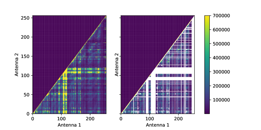
Figure 1: Amplitude diagnostics for all pairs of baselines before (left) and after (right) baseline flagging. Due to cross-talk between adjacent signal paths, a priori flagging of antennas adjacent to each other in the signal path has been applied before baseline flagging. The amplitude shown is the frequency-averaged amplitude after time averaging for $12$ hours without phase tracking. Therefore, outliers indicates bad antennas or baselines with excess stationary power. The final upgrade of the OVRO-LWA array will feature redesigned electronics with much better signal paths isolation and thus minimize signal coupling between nearby signal paths.

Flagging of bad data and calibration for this work largely follow the procedures outlined in Anderson et al. (2019), which we summarize here. For each day of observation, we identify and flag bad antennas from their autocorrelation spectra and derive the direction-independent (bandpass) calibration solutions during Cygnus A transit with the bandpass task in CASA 6 (McMullin et al., 2007; Raba et al., 2020). The bandpass calibration sets the flux scale. We then apply the daily bandpass solutions and flags to each $13$ s integration for the rest of the day. For each integration where Cyg A or Cas A are visible, we use TTCal(Eastwood, 2016), which implements the StEFCal algorithm (Salvini & Wijnholds, 2014), to solve for the their associated direction-dependent gains and and subtract their corrupted visibility from the data, a process known as peeling (Noordam, 2004). Peeling solutions are derived once per 13 s integration per 24 kHz frequency channel. Finally, for each integration, we find bad channels by detecting outliers in averaged visibilities per channel over baselines longer than 30 meters. The 30-meter cutoff suppresses flux contribution from the diffuse emission in the sky and allows for more robust outlier detections. The channel flags are subsequently applied to the $13$ s integration.

Our modifications to the Anderson et al. (2019) flagging and calibration approach are as follows:

1. Anderson et al. (2019) used 13 seconds of data during Cygnus A transit to derive the bandpass calibration. In this work, we use $20$ minutes of data around Cygnus A transit. The calibration integration time is longer than the typical ionospheric and analog gain fluctuation timescales of the array and thus offers more robust solutions that are more representative of the instrument bandpass.

2. To further identify baselines that have excess power due to cross-talk and common-mode noise, we follow Eastwood et al. (2018)’s strategy and derive baseline flags by identifying outliers in $12$ hour averaged visibility data without phase-tracking after bandpass calibration. We pick the 12 hours of the day when the the galaxy is below horizon. Averaging the visibility without phase-tracking attenuates the sky signals and highlights stationary excess power on baselines. Fig. 1 illustrates this strategy. These flags are generated and applied each day.

3. For each day, we randomly select two integrations to validate the flags and calibration solutions. We identify additional baselines and antennas that show excess visibility amplitude by visual inspection and add them to the per-day set of flags.

These flagging and calibration steps produce visibility data with flags at $13$ s time resolution.

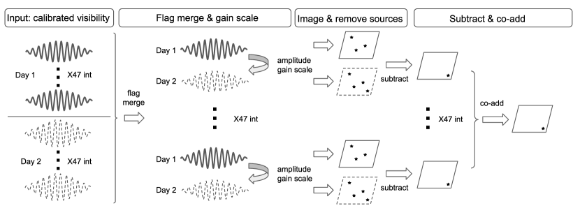
Figure 2: A cartoon representation of the imaging and differencing steps that produces the differenced images that we search for transients. The inputs are calibrated visibility from two time steps being subtracted, separated by one sidereal day. Each input visibility integration (represented by the fringe pattern) is 13 s long. The group of visibility data from each day consists of $47$ integrations. The flag merge, gain scale, imaging, source removal, subtract, and co-add steps are detailed in § 3.2

3.2 Imaging and Sidereal Image Differencing

In principle, image differencing allows us to remove diffuse emission and search for transients below the Jansky-level confusion limit (Cohen, 2004). However, when differencing OVRO-LWA images that were a few minutes apart, Anderson et al. (2019) observed the sensitivity degrading compared to the seconds-timescale search. They concluded that in searches for transients beyond a few integrations, sources’ motions across the antenna beams introduced significant direction-dependent errors that failed to subtract over the course of a few minutes.

Figure 3: Images illustrating effects that raise the noise level in sidereal image differencing and how we mitigate them. The rms noise is the rms noise reported by the source detection code. (a) The Sun moves by $\sim 1\deg$ per day. Deconvolving the Sun during imaging reduces the noise due to its sidelobes. (b) The analog gain scaling and inner Tukey weighting suppresses image differencing artifacts due to the diffuse sky, especially in the direction of the Galactic plane.

To circumvent the limitations due to the antenna beams, in this work we expand on the sidereal image differencing technique initiated by Anderson et al. (2019). We difference integrations that are, within $0.1$ s, 1 sidereal day apart, so that all persistent sources remain in the same positions of the antenna beams. Sidereal image differencing allows clean source subtraction without incorporating the individual antenna beams into calibration and imaging. This section details steps for generating $10$ min integrated and sidereally-differenced images (see also Fig. 2). For each pair of $10$ min groups of $13$ s visibility data that are 1 sidereal day apart, we perform the following operations:

1. We merge the flags for the two groups and apply the merged flags to all integrations within the groups. This ensures that the resultant images for the two groups have the same point spread function (PSF).

2. We apply a per-channel per-antenna per-integration amplitude correction to the integrations from the first day so that its autocorrelation amplitudes match those from the second day. This corrects for gain amplitude variations on short timescales (most notably temperature-dependent analog electronics gain variation that correlates with the $15$ min air-conditioning cycle in the electronics shelter).

3. We change the phase center of all visibility data to the same sky location, the phase center in the middle of the time integration. We then image each $13$ s integration with wsclean (Offringa et al., 2014), using Briggs $0$ weighting and a inner Tukey tapering parameter (-taper-inner-tukey) of 20 $\lambda$. The weighting and tapering scheme suppresses diffuse emission, especially toward the galactic plane, without introducing ripple-like artifacts corresponding to a sharp spatial scale cutoff. The typical full width at half maximum (FWHM) of the synthesized beam is $23^{\prime}\times 13^{\prime}$.

4. During imaging, we allow deconvolution of the Sun and the Crab pulsar by masking everything else in the sky with the -fits-mask argument of wsclean. We set the CLEAN threshold to $50$ Jy. This removes sidelobes in the images due to the Sun and the Crab pulsar: the Sun moves in celestial coordinates from day to day, and the Crab pulsar exhibits strong variability.

5. Each image from the first day is subtracted from its sidereal counterpart from the second day to form the differenced image. We then co-add the group of differenced images to form the $10$ min differenced image. We chose the co-adding approach because it is more efficient to parallelize than gridding all 10 minutes of visibility. For a subset of our data, we confirm that the co-added differenced images suffer from no sensitivity loss or artifacts by comparing them to differenced images produced directly by imaging the full $10$ min visibility dataset.

Figure 4: (a) Time series of noise at zenith in $10$ min subtracted images over the entire observation. Higher noise level corresponds to daytime. Noise level spikes typically occur at sunrise, at sunset, when a horizontal RFI source flares up, and when the Crab pulsar scintillates. (b) Histogram of image-plane noise measured in all integrations. The two modes of the distribution correspond to daytime (when both the Sun and the galactic plane are up) and nighttime observations.

Fig. 3 shows the main classes of problematic image differencing artifacts that our procedure removes. Our procedure aims at reducing the root-mean-square (rms) estimate of the noise due to far sidelobes of these artifacts in the rest of the image. The sidereally differenced images that our procedure produce are the data product on which we perform source detection to search for transients. Fig. 4 shows the noise characteristics of the sidereally differenced images.

We use Celery, a distributed task queue framework, with RabbitMQ as the message broker to distribute the compute workload for this project across a 10-node compute cluster near the telescope. Each node has $16$ cores and $64$ GB of RAM. The snapshot of the pipeline source code used for this work can be found at https://github.com/ovro-lwa/distributed-pipeline/tree/v0.1.0.

3.3 Source-finding and Candidate Sifting

We use the source detection code developed by Anderson et al. (2019) to detect sources in the sidereally subtracted images. The algorithm divides each image into $16$ tiles and estimates the local image noise in each tile. It then groups bright pixels with a Hierarchical Agglomerative Clustering (HAC) algorithm to identify individual sources. Anderson et al. (2019) tuned the parameters of the HAC algorithm for detecting sources in dirty subtracted images of the OVRO-LWA. The source detection algorithm only reports sources with peak flux density $6.5$ times the local standard deviation $\sigma$. Based on the number of independent synthesized beam searched (Frail et al., 2012), we estimate the probability of detecting a $6.5\sigma$ outlier due to Gaussian noise fluctuation over the entire survey to be $<5\times 10^{-3}$.

For each detected source, we visually inspect its cutout images and its all-sky image in an interactive Jupyter (Kluyver et al., 2016) notebook widget that records the labels for all detected sources. We developed the tool with the ipywidgets and matplotlib (Hunter, 2007) packages. We can rule out a large number of artifacts based on their appearances and their positions in the sky: RFI sources and meteor reflections are often resolved and/or close to the horizon. We label point sources detected in the subtracted images that only appear in either the “before” or the “after” images as candidate transients.

For these candidates, we generate spectra time series (dynamic spectrum) over the entire $58$ MHz of bandwidth and re-image them with different weighting schemes to ascertain the properties of these candidates. For candidates that appear near Vir A, Tau A, or Her A, we deconvolve the bright source to test whether a given candidate is part of the bright source’s sidelobe.

3.4 Quantifying Survey Sensitivity

We quantify the noise in subtracted images with the standard deviations at zenith reported by the source detection code.

The power beam of an OVRO-LWA dipole approximately follows a $\cos^{1.6}(\theta)$ pattern, where $\theta$ is the angle from zenith (Anderson et al., 2019). Therefore, for a given snapshot with noise at zenith $\sigma_{z}$, the primary-beam-corrected image noise at an angle $\theta$ from zenith is given by $\sigma_{z}/\cos^{1.6}(\theta)$. Furthermore, the number of artifacts increases as the zenith angle increases, due to both horizon RFI sources and increased total electron content (TEC) through the ionosphere at lower elevations. Therefore, we define the zenith angle cutoff for our survey as when the marginal volume probed with increasing zenith angle is small. The volume probed for a non-evolving population of transients uniformly distributed in space has the following dependencies on FOV and sensitivity:

$$V\propto\int_{0}^{\theta_{0}}S_{0}^{-3/2}d\Omega,$$ (1)

where $S_{0}$ is the sensitivity as a function of solid angle $\Omega$, and $\theta_{0}$ the zenith angle limit of a survey. This is equivalent to the Figure of Merit defined in Macquart (2014) for such a population of transients. Substitute in the dependency of sensitivity on zenith angle and we get

$$V \propto \int_{0}^{\theta_{0}}(\cos^{-1.6}{\theta})^{-3/2}\sin{\theta}d\theta$$

$$\propto -\cos^{3.4}\theta_{0}.$$

We choose a zenith angle cut $\theta_{0}=60\deg$, which encompasses $90\%$ of the available survey volume. The beam-averaged noise $\bar{\sigma}$ is therefore given by

$$\bar{\sigma}=\frac{\int_{0}^{2\pi}\int_{0}^{\theta_{0}}\frac{\sigma_{z}}{\cos^{1.6}\theta}\sin\theta d\theta d\phi}{\int_{0}^{2\pi}\int_{0}^{\theta_{0}}\sin\theta d\theta d\phi}.$$ (2)

For a zenith angle cut of $\theta_{0}=60\deg$, this evaluates to $1.72\sigma_{z}$.

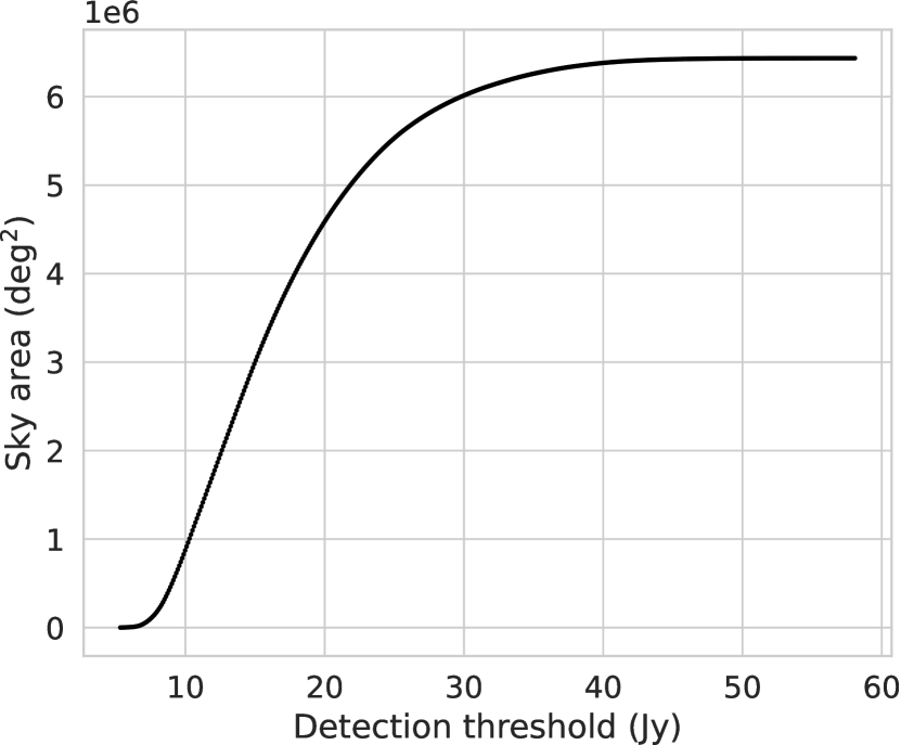
Figure 5: Cumulative sky area surveyed at $10$ min timescale as a function of detection threshold.

Since our sensitivity varies significantly over the FOV, we also quantify our sensitivity in terms of total sky area versus sensitivity, aggregated over all images in our survey. Our approach is similar to that of Bell et al. (2014), albeit with much finer flux density bins. Fig. 5 shows the cumulative sky area as a function of sensitivity for $10$ min timescale transients. The binned sky area and sensitivity $\{\Omega_{tot,i},S_{i}\}$ forms the basis of our Bayesian modeling of transient detections detailed in § 4.2.

The aforementioned approach assumes that the sky is static with respect to the primary beam. However, Earth rotation rotates the sky across the primary beam. We do not account for for this effect in our analysis due to the short integration time and the smoothness of the primary beam. The rotation modifies the sensitivity estimate for each point in the sky by a negligible $<1\%$ for a 10 min integration.

4 Estimating the Transient Surface Density

While our survey aims to match Stewart et al. (2016) as much as possible, there remains a number of differences. Most notably, our sensitivity varies by factor of $\sim 8$ across the survey, due to the gain pattern of a dipole antenna and different level of sky noise at different time of the day. Therefore, in this section, we devise a Bayesian scheme for inferring transient rates so that we can incorporate varying sensitivity as a function of sky area surveyed. The Bayesian approach also facilitates testing whether two survey results are consistent, an important question when the implied rate of two surveys are significantly different.

4.1 The Frequentist Confidence Interval

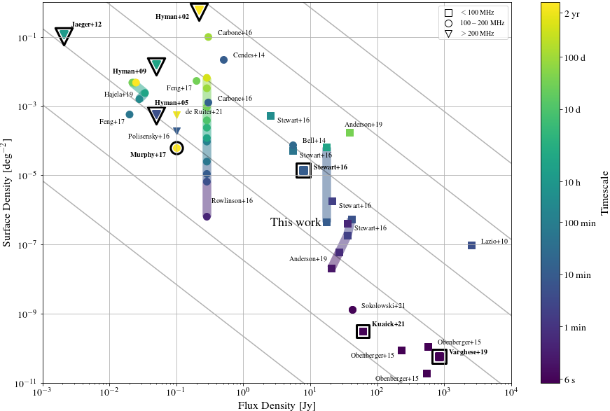
Figure 6: The radio transient phase space diagram shows the transient surface density as a function of limiting flux density for non-targeted transient surveys at $<300$ MHz to date. Each point denotes the typical sensitivity and the $95\%$ frequentist upper limit of transient surface density of the survey. Surveys with detections are marked in bold. The color denotes the timescale of the search, ranging from timescales of $1$ s (Kuiack et al., 2021a) to $5.5$ -yr (de Ruiter et al., 2021). Surveys conducted at different frequencies are marked with different shapes. Surveys with similar surface density and flux density limits may probe different populations of transients if they operate in different frequencies or timescales. Each of the solid gray lines traces a hypothetical standard candle population in a Euclidean universe, i.e. a cumulative flux density distribution (Eq. 6) power law index of $\gamma=3/2$.
References: Hyman et al. (2002, 2005, 2009); Lazio et al. (2010); Jaeger et al. (2012); Bell et al. (2014); Cendes et al. (2014); Obenberger et al. (2015); Carbone et al. (2016); Polisensky et al. (2016); Rowlinson et al. (2016); Stewart et al. (2016); Feng et al. (2017); Murphy et al. (2017); Anderson et al. (2019); Hajela et al. (2019); Varghese et al. (2019); Kuiack et al. (2021a); de Ruiter et al. (2021); Sokolowski et al. (2021).

Once we count the number of transients $n$ detected in a survey, we can estimate the rate of low-frequency transients. For a given timescale, the rate of transients above a certain flux density threshold $S_{0}$ is typically parameterized by the surface density $\rho$, which gives the number of transients per sky area. For a given population of transient that occur with a surface density $\rho$ above a certain flux threshold $S_{0}$, the number of detections in a given survey with total independent sky area surveyed $\Omega_{tot}$ follows a Poisson distribution with rate parameter

$$\lambda=\rho\Omega_{tot}.$$ (3)

The probability mass function (PMF) of the Poisson distribution is given by

$$P_{pois}(n|\lambda)=\frac{\lambda^{n}e^{-\lambda}}{n!},$$ (4)

where $P(n)$ is the probability of obtaining $n$ detections. Gehrels (1986) computed a table of confidence interval values for $\lambda$ for a range of probability and number of detections in a given survey, from which one can derive the confidence interval on the surface density $\rho$. The 95% upper limit on the surface density $\rho$, along with the survey sensitivity $S_{0}$, is the typical metric quoted in low-frequency radio transient surveys and are plotted in the phase space diagram (Fig. 6).

Our survey is sensitive to transients with decoherence timescale (Macquart, 2014) $T$ from $10$ minutes to $1$ day. Since each of our snapshot has the same FOV $\Omega_{FOV}$, the total independent sky area surveyed is given by

$$\Omega_{tot}\simeq\Omega_{FOV}\left\lfloor\frac{N}{T/10\text{min}}\right\rfloor,$$ (5)

where $N$ is the number of $10$ min sidereally differenced images and $\lfloor\cdot\rfloor$ the floor function. Following conventions in the low-frequency transient search literature, we quote the $95\%$ confidence upper limit on $\rho$ at the average sensitivity of the survey.

4.2 Bayesian Inference for Transient Surveys

For wide-field instruments at low frequencies, the survey sensitivity can vary by more than an order of magnitude with time and FOV. Different sensitivity probes a different depth for a given population of transients. By reducing the information contained in a survey to its typical sensitivity, the above approach does not use all information contained within a survey. To address the variation of sensitivity across a survey, Carbone et al. (2016) models the surface density $\rho$ above a flux threshold $S_{0}$ as a power law of sensitivity:

$$\rho(S>S_{0})=\rho_{*}\left(\frac{S_{0}}{S_{*}}\right)^{-\gamma},$$ (6)

where $\gamma$ is the power law index, and $\rho_{*}$ the reference surface density at flux density $S_{*}$. The Poisson rate parameter is then given by

$$\lambda=\rho_{*}\left(\frac{S_{0}}{S_{*}}\right)^{-\gamma}\Omega_{tot},$$ (7)

For a given $\gamma$, the reference surface density $\rho_{*}$ can be inferred from number of detections in parts of the survey with different sensitivity.

Here we develop a Bayesian approach that extends the Carbone et al. (2016) model. Apart from enabling future extensions to the model, the main utilities of the Bayesian approach are as follows:

1. it allows us to marginalize over the source count power law index $\gamma$ for an unknown population when inferring the surface density $\rho_{*}$;

2. it outputs posterior distribution over $\rho_{*}$, which can be integrated to inform future survey decision making;

3. it allows for robust hypothesis testing of whether survey results are consistent with each other.

Our baseline model, $\mathcal{M}_{1}$, jointly infers $\gamma$ and $\rho_{*}$ for a single population of transients, thereby naturally accommodating our survey’s change of surface area with sensitivity. The alternative model, $\mathcal{M}_{2}$, proposes that our survey probes a population with surface density $r\rho_{*}$, with $r$ as a free parameter. In other words, $\mathcal{M}_{2}$ proposes that our survey and Stewart et al. (2016) select for different population of transients. Model comparison between $\mathcal{M}_{1}$ and $\mathcal{M}_{2}$ informs us whether two transient surveys yield inconsistent results. We now elaborate on the details of the models. The notebooks that implement the models are hosted at https://github.com/yupinghuang/BIRTS.

4.2.1 The Setting

To infer the model parameters $\bm{\theta}$ for a given model $\mathcal{M}$ and measured data $D$, we use Bayes’ theorem to obtain the posterior distribution, the probability distribution of $\bm{\theta}$ given the data,

$$p(\bm{\theta}|D,\mathcal{M})=\frac{p(D|\bm{\theta},\mathcal{M})p(\bm{\theta}|\mathcal{M})}{p(D|\mathcal{M})}.$$ (8)

Several other probability distributions of interest appear in Bayes’ theorem. $p(D|\bm{\theta},\mathcal{M})$ is the likelihood function, the probability of obtaining the measured data $D$ given a fixed model parameter vector $\bm{\theta}$ under model $\mathcal{M}$. $p(\bm{\theta}|\mathcal{M})$ is the prior distribution, specifying our a priori belief about the parameters. $p(D|\mathcal{M})$ is the evidence, the likelihood of observing data $D$ under model $\mathcal{M}$. Normalization of probability to $1$ requires that

$$p(D|\mathcal{M})=\int p(D|\bm{\theta},\mathcal{M})p(\bm{\theta}|\mathcal{M})d\bm{\theta},$$ (9)

which gives the evidence $p(D|\mathcal{M})$ the interpretation of the likelihood of observing data $p(D)$ averaged over the model parameter space.

4.2.2 Representing Data

We encode the results of surveys in the data variable $\{D_{i}\}=\{S_{0,i},\Omega_{tot,i},n_{i}\}$, where ${S_{0,i}}$ are the sensitivity bins, $\Omega_{tot,i}$ the differential total area surveyed in the $i$-th bin, and $n_{i}$ the number of detections in the $i$-th bin. The Stewart et al. (2016) detection with LOFAR can then be written as a one-bin data point:

$$D_{L}=\{15~{}\text{Jy},3.3\times 10^{5}~{}\deg^{2},1\}.$$ (10)

For the OVRO-LWA, $\{S_{0,i},\Omega_{tot,i}\}$ is the differential sensitivity-sky area curve described in § 3.4.

4.2.3 A Single Population Model

For a single survey, or for multiple surveys where we assume that the selection criteria do not affect the observed rate of the transients, a Poisson model with a single reference surface density $\rho_{*}$ and source count power law index $\gamma$ is appropriate. We denote this model $\mathcal{M}_{1}$ and the parameters $\bm{\theta_{1}}=(\rho_{*},\gamma)$.

For all the survey data encoded in $\{D_{i}\}$, the model states that for each sensitivity bin $S_{0,i}$ with sky area $\Omega_{tot,i}$, the detection count $n_{i}$ follows a Poisson distribution

$$\mathcal{M}_{1}:n_{i}\sim P_{pois}\left(n_{i}|\lambda=\rho_{*}\left(\frac{S_{0,i}}{S_{*}}\right)^{-\gamma}\Omega_{tot,i}\right),$$ (11)

where we use the $\sim$ operator to denote that each $n_{i}$ independently follows the distribution specified by the Poisson PMF $P_{pois}$ defined in Eq. 4. We choose the reference flux density $S_{*}=15$ Jy.

With the model specified, we adopt uninformative prior distributions $p(\gamma)\propto\gamma^{-3/2}$ and $p(\rho_{*})\propto 1/\rho_{*}$ derived in Appendix A. Integrating the joint posterior distribution $p(\rho_{*},\gamma|D,\mathcal{M}_{1})$ gives the marginalized posterior distribution for $\rho_{*}$. To understand the sensitivity of the posterior distribution on the choice of prior distributions, we also derive the posterior with uniform priors on $\gamma$ and $\rho_{*}$. In all cases, we bound the prior distribution on on $\gamma$ to $(0,5)$ and on $\rho_{*}$ to be $(10^{-14},10^{-3})\deg^{-2}$.

Even though the Poisson distribution can be integrated analytically over $\lambda$, with our modifications the likelihood function cannot be integrated analytically. For this two-parameter model, the integral can be done by a Riemann sum over a grid. However, we adopt a Markov Chain Monte Carlo (MCMC) approach to integrate the posterior distribution. The MCMC approach allows extensions of the model. For example, one may wish to incorporate an upper flux density cutoff $F_{max}$, for the flux density distribution. We extend this model to test the consistency of different survey results in the next section. The MCMC approach will also allow future work to turn more realistic models for transient detections (see e.g. Carbone et al., 2017; Trott et al., 2013, and references within) into inference problems, which will enable more accurate characterizations of the transient sky.

We use the No-U-Turn Sampler (NUTS; Hoffman et al., 2014), an efficient variant of the Hamiltonian Monte Carlo (HMC; Duane et al., 1987) implemented in the Bayesian inference package pymc3 (Salvatier et al., 2016) to sample from the posterior distribution. We allow 5000 tuning steps for the NUTS sampler to adapt its parameters and run 4 chains at different starting points. We check the effective sample size and the $\hat{R}$ statstics (Vehtari et al., 2021) provided by pymc3 for convergence of the samples to the posterior distribution.

4.2.4 A Two-population Model

To answer whether our survey results are consistent with Stewart et al. (2016), we develop a second model $\mathcal{M}_{2}$ as the competing hypothesis. $\mathcal{M}_{2}$ states that the transient counts from our survey with the OVRO-LWA, $\{n_{i}\}_{O}$, are drawn from a different Poisson distribution from which the LOFAR counts $\{n_{i}\}_{L}$ are drawn from. We introduce the surface density ratio, $r$, which modifies the effective transient surface density $\rho_{*}$ for our survey. In other words, $\mathcal{M}_{2}$ posits that our survey probes a population with a different surface density $r\rho_{*}$, than did Stewart et al. (2016). The model can be written as

$$\mathcal{M}_{2}:$$

$$\{n_{i}\}_{L}\sim P_{pois}\left(n_{i}|\lambda=\rho_{*}\left(\frac{S_{0,i}}{S_{*}}\right)^{-\gamma}\Omega_{tot,i}\right),$$

$$\{n_{i}\}_{O}\sim P_{pois}\left(n_{i}|\lambda=r\rho_{*}\left(\frac{S_{0,i}}{S_{*}}\right)^{-\gamma}\Omega_{tot,i}\right).$$ (12)

Our physical interpretation of $\mathcal{M}_{2}$ is that the two surveys probe populations with different averaged transient surface density.

The parametrization with the surface density ratio $r$ captures a wide range of selection effects, which may result in different specifications of the prior distribution on $r$. Since our survey covers the galactic plane, our all-sky rate can be enhanced if the population is concentrated along the galactic plane. We speculate that a natural prior on $r$ is then a uniform prior. On the other hand, the time sampling of Stewart et al. (2016) extends over $4$ months, while we have a continuous $5$ day survey. If the decoherence timescale of the transient event is much longer than the $10$ min emission timescale (e.g. long-term activity cycles), it reduces the number of epochs and thus the effective total area $\Omega_{tot}$ for our survey. In this case, a uniform prior on $1/r$ might be more appropriate. Lacking compelling evidence, we do not assume a particular source of rate modification and prefer the uninformative prior $p(r)\propto 1/r$ derived in Appendix A, which is invariant under the reparameterization $r\rightarrow 1/r$. Finally, we can put an additional constraint of $r>1$ or $r<1$ on the prior depending on whether we are interested in testing the effective surface density in our survey is enriched or diluted.

This parameterization, however, does not capture narrow bandwidth of the signal, because a narrow bandwidth modifies the effective flux of the transient, which appears inside the exponentiation by $\gamma$ in Eq. 7. Since we explicitly search for narrowband transients (§ 2), we do not consider such a model.

4.2.5 Testing Survey Consistencies via Model Comparison

With the two models we developed, the question of whether two survey results are inconsistent translates to deciding which model is preferred given the data. Given the dearth of information contained in surveys with few or no detections, a particular class of methods may inadvertently bias the result. Therefore, we test three different methods for Bayesian model comparisons as outlined below and compare their results.

WAIC

The first class is based on estimating the predictive accuracy of models. One popular example is the Widely Applicable Information Criterion (WAIC; Watanabe, 2013; Vehtari et al., 2015), which can be easily computed from posterior samples. Given $S$ samples of the parameters $\bm{\theta_{s}}$ from the computed posterior and all the data $y_{i}$, the WAIC is given by

$$\text{WAIC}= \sum_{i=1}^{n} \log\left(\frac{1}{S}\sum_{s=1}^{S}p(y_{i}|\bm{\theta_{s}})\right)-$$ (13)

$$\sum_{i=1}^{n} \text{Var}_{s=1}^{S}(\log p(y_{i}|\bm{\theta_{s}})),$$ (14)

where $\text{Var}_{s=1}^{S}$ denotes variance taken over the posterior samples. The first term is an estimate of the expected predictive accuracy of the model, while the second term, the effective degree of freedom, penalizes more complex models that are overfitted. The difference in the WAIC between two models, $\Delta\text{WAIC}$, then gives a measure of how well the two models may predict out-of-sample data.

Bayes factor

The second class of model comparison method bases on the Bayesian evidence Eq. 9, i.e. how efficient does a model explain observed data. Between two models, one computes the Bayes factor

$$B_{12}=\frac{p(\mathcal{M}_{1}|D)p(\mathcal{M}_{1})}{p(\mathcal{M}_{2}|D)p(\mathcal{M}_{2})},$$ (15)

where $p(\mathcal{M}_{1})$, and $p(\mathcal{M}_{2})$ are the prior distributions on each model, usually taken to be equal when no model is preferred a priori. Models with a larger parameter space is penalized by the resultant lower prior density. Scales exist for interpreting the significance of Bayes factor (Kass & Raftery, 1995).

Mixture model

The third method advocates for the use of a mixture model of the two contesting models in question and basing model comparison off the posterior of the mixture parameter (Kamary et al., 2014). The mixture approach avoids the computational cost and some theoretical difficulties of the Bayes factor. To construct the mixture model, we refer to the distribution function that generates the data under $\mathcal{M}_{1}$ as $f_{1}$, and the distribution function that corresponds to $\mathcal{M}_{2}$ as $f_{2}$, such that Eq. 11 is equivalently $\mathcal{M}_{1}:n_{i}\sim f_{1}$, and Eq. 4.2.4 is $\mathcal{M}_{2}:n_{i}\sim f_{2}$. With a parameter $\alpha$ that denotes the mixture weight for model $\mathcal{M}_{2}$, $0\leq\alpha\leq 1$. We construct the mixture model $\mathcal{M}_{m}$ from $\mathcal{M}_{1}$ and $\mathcal{M}_{2}$ for the purpose of model comparison. $\mathcal{M}_{m}$ is given by

$$\mathcal{M}_{m}:n_{i}\sim(1-\alpha) f_{1} (n_{i}|\bm{\theta_{1}},\Omega_{tot,i},S_{0,i})+$$

$$\alpha f_{2} (n_{i}|\bm{\theta_{2}},\Omega_{tot,i},S_{0,i}).$$ (16)

The mixture weight, $\alpha$, can be interpreted as the propensity of the data to support $\mathcal{M}_{2}$ versus $\mathcal{M}_{1}$. If $\alpha\rightarrow 1$, then $\mathcal{M}_{2}$ generates the data. If $\alpha\rightarrow 0$, $\mathcal{M}_{1}$ generates the data. Kamary et al. (2014) shows that the posterior distribution of $\alpha$ asymptotically concentrates around the value corresponding to the true model and recommend the posterior median $\hat{\alpha}$ as the point estimate for $\alpha$. We adopt Beta$(0.5,0.5)$ as the prior for the mixture weight $\alpha$, per the recommendation of Kamary et al. (2014). Beta$(0.5,0.5)$ equally encourages the posterior density of $\alpha$ to concentrate around $0$ and $1$. We also test the sensitivity of our results to the prior on $\alpha$ by using a uniform prior on $\alpha$.

Implementation

We compute $\Delta_{\text{WAIC}}$ and its standard deviation from the HMC posterior samples for $\mathcal{M}_{1}$ and $\mathcal{M}_{2}$. Given the low dimensionality of the model, we are able to compute the Bayes factor with the Sequential Monte Carlo algorithm (Ching & Chen, 2007; Minson et al., 2013) implemented in pymc3. We implement the mixture model as a separate model in pymc3 and sample from the posterior with the HMC algorithm to infer the mixture weight $\alpha$. We obtain the median of the posterior distribution of $\alpha$ and visually examine the posterior for concentration of probability density around $0$ or $1$. We present and interpret these model selection metrics in § 5.3.

5 Results

Figure 7: Diagnostics of the unresolved reflection candidate OLWA J1436+5103. (a) Discovery images of the candidate from the $722$ kHz wide search. The three panels show the differenced image, the image from the day before, and the image when the source appears. The title text displays the date of occurrence, the coordinates, the flux density, S/N, and distance to closest match in the persistent source catalog. (b) Dynamic spectrum for the $10$ min integration within a single $2.6$ MHz subband. The source is confined within a single time integration and only part of the subband bandwidth. (c) Spectrum of the source across the full $58$ MHz bandwidth in the single integration when the source is bright. The shaded region indicates broadcast frequencies of Channel 3 television. The coincidence of the emission frequencies with Channel 3 TV broadcast frequencies point to this source as a reflection artifact, likely from a meteor.

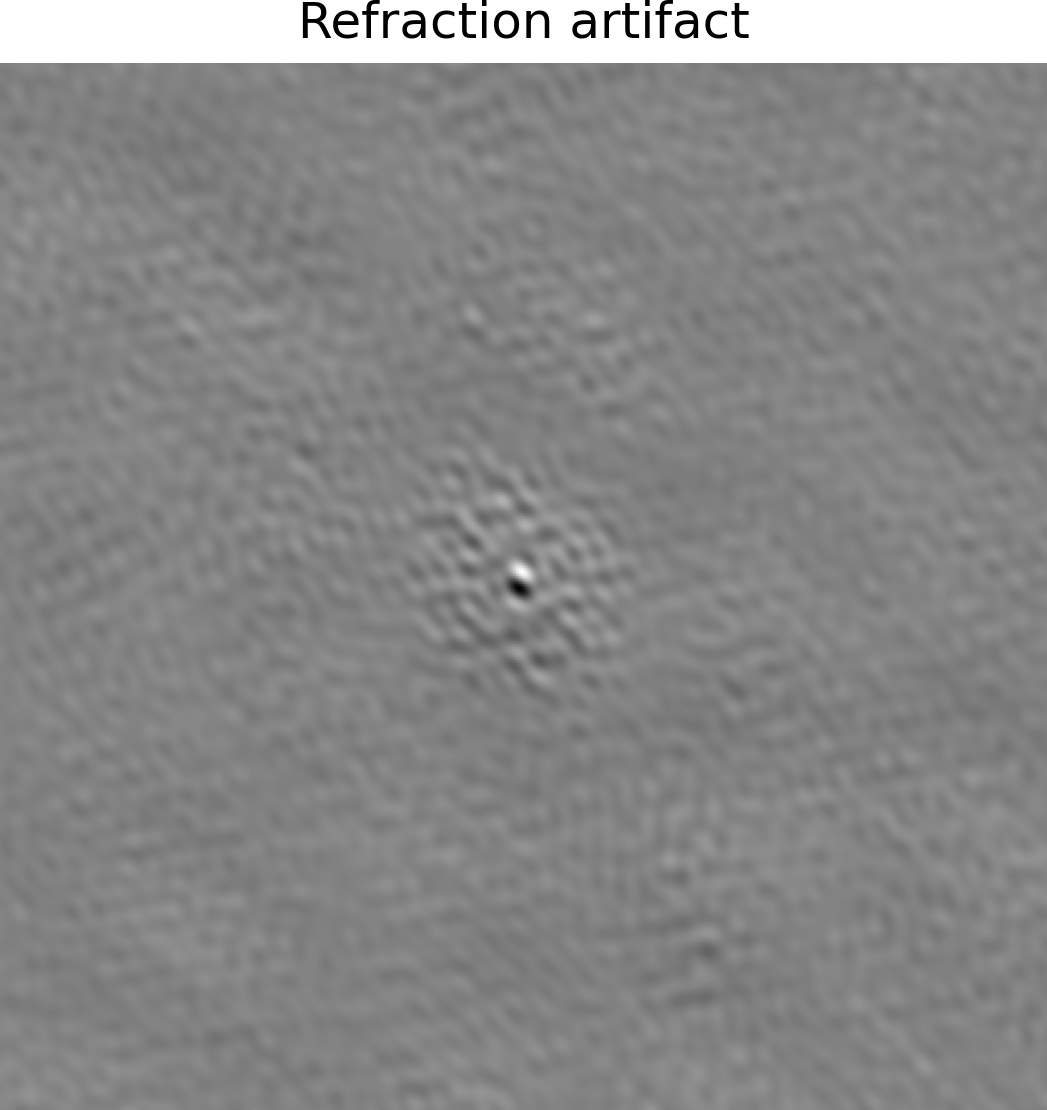
Figure 8: An example of refraction artifact in a differenced image. The position offset of the source between the two images gives rise to the dipole pattern in the differenced image.

5.1 Artifacts

Table 2: Number of transient candidates remaining after each major vetting step of the transient detection pipeline

Search step	Detection count
Source detection	9057
Persistent-source matching	2317
Visual inspection	2
Re-imaging	0

Table 2 shows the number of transient candidates after each sifting step. All $9057$ detected sources turned out to be artifacts. All of the artifact classes detailed in Anderson et al. (2019) appear in our data: meteor reflections, airplanes, horizon RFI sources, and scintillating sources. Fig. 7 shows a bright meteor reflection candidate, which appears as an unresolved source in the image. In addition to the artifacts detailed in Anderson et al. (2019), we identify $2$ classes of artifacts that are unique to our sidereal differencing search with long integration time: refraction artifacts and spurious point-like sources near the NCP.

The first class of artifacts that we identify is refraction artifacts (also described in Kassim et al., 2007). The bulk ionosphere functions as a spherical lens for a wide-field array (Vedantham et al., 2014). Due to the difference in the bulk ionospheric content between two images that are $1$ day apart, sources are refracted by different amounts in the two images and result in artifacts that have a dipole shape in the subtracted images (see Fig. 8 for an example). We identify these artifacts by visual inspection and by cross-matching detections against the persistent source catalog generated as a by-product of Anderson et al. (2019). However, for more sensitive searches in the future, the number of refraction artifacts will increase; collectively, their sidelobes may raise the noise level significantly. Image-plane de-distortion techniques like fits_warp (Hurley-Walker & Hancock, 2018) and direct measurement & removal techniques (see e.g. Reiss, 2016) can be used to suppress these refraction artifacts and their sidelobes in future searches, provided that the ionospheric phase remains coherent across the array.

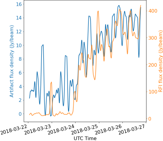
Figure 9: Light curves of the point source artifact at $\delta=86^{\circ}$ and the horizon RFI source. The flux scale for the artifact is on the left vertical axis and the flux scale for the horizon RFI source on the right. The light curves of these two sources are correlated.

The second class of artifacts is spurious point sources near the NCP. Two prominent sources, one at $\delta=86^{\circ}$ and the other at $\delta=76^{\circ}$, were repeatedly detected. Their flux density values correlate with that of a source of RFI in the northwest, which we attribute to an arcing power line (Fig. 9). For a long integration time, the slow fringe rate near the NCP may allow low-level near-field RFI sources and their sidelobes to show up as point-like sources (Perley, 2002; Offringa et al., 2013a). For this reason, we exclude the $15^{\circ}$ radius around the NCP from our subsequent analyses.

We note that even though the Stewart et al. (2016) survey centered on the NCP and they did not test for an RFI source outside their $10\deg$ FOV, it is unlikely that their detection is a sidelobe of a source of RFI. Unlike the OVRO-LWA, which cross-correlates all dipole antennas, LOFAR first beamforms on the station level (each station consisting of $96$ signal paths, typically 48 dual-polarization antennas) and then cross-correlates voltages from different stations. The station-based beamforming approach suppresses sensitivity to sources outside the main beam. In addition, although all the individual LOFAR dipole antennas are aligned, the antenna configurations of the Dutch LOFAR stations are rotated with respect to each other (van Haarlem et al., 2013), making it even less likely for the pair of stations in each baseline to be sensitive to the same direction far beyond the main beam. Finally, deep LOFAR observations of the NCP did not reveal RFI artifacts (Offringa et al., 2013b). Therefore, despite the high declination of the Stewart et al. (2016) survey field, we conclude that the sidelobe of a horizon RFI source likely did not lead to their transient detection.

5.2 Limits on Transient Surface Density

Table 3: Sky area per detection threshold bin at $10$ min timescale

Detection threshold (Jy)	Sky area (deg2)
5.33	242.36
5.44	381.59
5.54	479.56
5.65	835.37
…	…
58.07	14.1

Note. — Table 3 is published in its entirety in the machine-readable format. A portion is shown here for guidance regarding its form and content.

Fig. 4 illustrates the noise characteristics of the survey. Across the survey, the mean noise level in subtracted images is $1.57$ Jy with a standard deviation of $0.39$ Jy. Given our $6.5\sigma$ detection threshold, the mean noise level translates to a sensitivity of $10$ Jy at zenith. The cumulative sky area surveyed as a function of sensitivity is shown in Fig. 5, with the differential area per sensitivity bin recorded in Table. 3. As we find no astrophysical transient candidates in our search, we seek to put an upper limit in the transient surface density-flux density phase space. Our search is done with sidereal image differencing with an integration time of $10$ minutes. The number of sidereally differenced $10$ min images $N$ (Eq. 5) is $N=659$ after flagging integrations with excessive noise.

Because we exclude the sky area with declination above $75\deg$ and altitude angle below $30\deg$, we calculate the snapshot FOV and the FOV-averaged sensitivity numerically. We begin with a grid defined by the cosine of the zenith angle, $\cos\theta$, and the azimuth angle, $\phi$, such that each grid cell has the same solid angle $\Omega$. We then exclude cells that do not satisfy our declination cut. Finally, we evaluate the total solid angle integral $\Omega=\int\int(d\cos\theta)d\phi$ and the beam-averaging integral (Eq. 2) by a Riemann sum over the remaining grid cells. We find that the effective snapshot FOV for our survey is $\Omega_{FOV}=9800\deg^{2}$ and the FOV-averaged sensitivity is $1.7\sigma_{z}$.

Therefore, for a given population of transients with timescale $T$ from $10$ min to $1$ day, the total sky area searched for a transient with timescale $T$ is

$$\Omega_{tot} = \left.\Omega_{FOV}N\middle/\left\lfloor\frac{T}{10\text{min}}\right\rfloor\right.$$ (17)

$$= \left.6.5\times 10^{6}\middle/\left\lfloor\frac{T}{10\text{min}}\right\rfloor\right.\deg^{2}.$$

We found no $10$ min transients at an averaged sensitivity of $S_{0}=17$ Jy. At this flux level, we apply the approach described in § 6 and place a $95\%$ confidence frequentist limit on the transient surface density at

$$\rho\leq 4.6\times 10^{-7}\left\lceil\frac{T}{10\text{min}}\right\rceil\deg^{-2}.$$ (18)

We place our limits in the context of other surveys at similar frequencies in Fig. 6. Even though our upper limit is a factor of 30 more stringent than that of Stewart et al. (2016), our upper limit is marginally consistent with their 95% confidence lower limit of $1.5\times 10^{-7}\deg^{-2}$ at $11$ min timescale and $15$ Jy.

We apply our Bayesian model $\mathcal{M}_{1}$ to the detection threshold-sky area data (Table. 3). The model jointly infers the flux density distribution power law index $\gamma$ and the reference surface density at $15$ Jy, $\rho_{*}$, because our survey probes different amount of volume depending on $\gamma$. The estimate on $\rho_{*}$ is averaged over the prior on $\gamma$. In the uninformative prior case, the posterior distribution of $\rho_{*}$ is dominated by the prior for much of the probability density because the data do not contain much information. We report a $99.7\%$ credible upper limit of $2.1\times 10^{-7}\deg^{-2}$, at which point the posterior distribution has deviated from the prior significantly. In the case of a uniform prior over $(0,5)$ on $\gamma$ and flat prior on $\rho_{*}$, we find a $95\%$ credible upper limit of $3.9\times 10^{-7}\deg^{-2}$ and a $99.7\%$ credible upper limit of $8.2\times 10^{-7}\deg^{-2}$.

5.3 Consistency with Stewart et al. (2016)

Table 4: Survey parameters of this work with comparisons to the previous OVRO-LWA survey (Anderson et al., 2019) and Stewart et al. (2016) at relevant timescale

	This work	Anderson et al. (2019)	Stewart et al. (2016)
Timescale	611 s – 1 day	13 s – 1 day	30s, 2 min, 11 min, 55 min, 297 min
Central frequency (MHz)	$60$	$56$	$60$
Bandwidth (kHz)	$744$	$58000$	$195$
Resolution (arcmin)	$23\times 13$	$29\times 13.5$	$5.4\times 2.3$
Total observing time (hours)	137	31	348
Snapshot FOV ($\deg^{2}$)	$9800$	$17,045$	$175$
Average rms (Jy/beam)	$1.57$	$1.68$	$0.79$
95% surface density upper limit ($\deg^{-2}$)	$4.6\times 10^{-7}$	$5.53\times 10^{-7}$	$1.4\times 10^{-5}$
95% surface density lower limit ($\deg^{-2}$)	-	-	$1.5\times 10^{-7}$

Table 4 compares the parameters of our survey to Stewart et al. (2016) and Anderson et al. (2019). Our survey features a similar bandwidth, sensitivity, and timescale as the transient ILT J225347+862146. We ask whether our results are consistent with the Stewart et al. (2016) detection in a Bayesian model comparison setting. We consider the Stewart et al. (2016) detection as a data point $D_{L}$ (Eq. 10), and our survey as a collection of data points $\{D_{O,i}\}$ given by Table 3. Model $\mathcal{M}_{1}$ posits that both observations can be explained by a single population, whereas $\mathcal{M}_{2}$ posits that our survey’s selection effect results in a reduced transient rate (or equivalently, that our survey probes a different population with a reduced surface density). We consider the WAIC, the Bayes factor $B_{12}$, and the mixture model parameter $\alpha$ as three separate tests. We vary the prior on the surface density ratio $r$ and show the metrics in Table. 5.

Table 5: Model comparison metrics between the single rate model, $\mathcal{M}_{1}$, and the two-rate model, $\mathcal{M}_{2}$, with different priors on the rate ratio $r$ for the OVRO-LWA survey. $\Delta{\text{WAIC}}_{12}$ is the difference in WAIC, $\sigma_{\Delta{\text{WAIC}},12}$ its uncertainty, $B_{12}$ the Bayes factor, and $\hat{\alpha}$ the posterior median of the mixture weight. In all cases we additionally bound $0<r<1$ due to our non-detection. Larger values of $\Delta{\text{WAIC}}_{12}$, $B_{12}$, and $\hat{\alpha}$ mean greater preference for $\mathcal{M}_{2}$ relative to $\mathcal{M}_{1}$.

Prior	Predictive Accuracy		Bayes Factor	Mixture Model
	ΔWAIC_12	σ_ΔWAIC,12	B_12	^α
r∼Uniform(0,1)	1.6	1.3	3.53	0.78
p(r)∝1/r	4.0	3.1	28.8	0.97
1/r∼Uniform(1,2×10^4)	4.1	3.1	31.8	0.97

For all the priors we chose for $r$, the difference in WAIC, which estimates the predictive power of each model, is comparable to its standard deviation estimated across all data. The high standard error estimate is consistent with the fact that all but one data point, the detection, contain very little information. The WAIC test is therefore inconclusive.

We are able to compute the Bayes factor with good precision, as estimated from the results from multiple parallel MCMC chains. The Bayes factor gives the ratio of the posterior probability of each model. In our case where we assume the prior probability on each model to be equal, the Bayes factor corresponds to the ratio of the likelihoods of observing the data under each of the two models. The only addition in model $\mathcal{M}_{2}$ compared to $\mathcal{M}_{1}$ is the surface density ratio $r$ for our survey relative to Stewart et al. (2016). We compute the Bayes factor for different prior distributions over $r$. We rely on the scale suggested by Kass & Raftery (1995), which categorizes the Bayes factor significance as “not worth more than a bare mention” ($0<\log(B_{12})<1/2$), “substantial” ($1/2<\log(B_{12})<1$), “strong” ($1<\log(B_{12})<2$), and “decisive” ($\log(B_{12})>2$), to interpret the Bayes factor $B_{12}$. The uniform prior on $r$ model presents “substantial” evidence, the uninformative prior model “strong”, and uniform prior on $1/r$ model “strong” evidence that $\mathcal{M}_{2}$ is preferred. Although the Bayes factor varies by up to an order of magnitude with the choice of prior, in all cases the Bayes factor prefers $\mathcal{M}_{2}$. Therefore, we conclude that the Bayes factor test prefers the two-population model, $\mathcal{M}_{2}$.

The mixture weight $\alpha$ tells a similar story as the Bayes factor. Fig. 10 shows a sample posterior distribution of $\alpha$. For all of the $\mathcal{M}_{2}$ variants, the posterior distribution of $\alpha$ concentrates toward $1$, exhibiting a preference for $\mathcal{M}_{2}$ (Kamary et al., 2014). All of the posterior median estimates for $\alpha$, $\hat{\alpha}$ are close to $1$. We draw identical conclusions in the case when the prior on $\alpha$ is uniform as well, but only show results for the prior $\alpha\sim$Beta$(0.5,0.5)$.

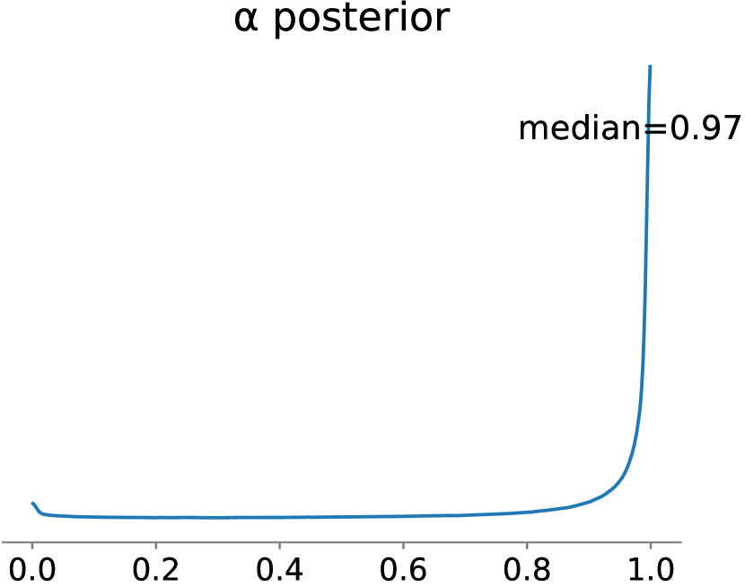
Figure 10: Posterior distribution of the mixture weight $\alpha$ with uninformative prior on all parameters. We adopt the posterior median $0.94$ to be the point estimate for $\alpha$. The posterior concentrates toward $\alpha=1$, indicating a preference for the model $\mathcal{M}_{2}$.

In the tests that are conclusive, we find strong evidence in support of the model $\mathcal{M}_{2}$, suggesting that our non-detection is not consistent with Stewart et al. (2016) under a single Poisson population model. Since we did not have a detection, our goal for testing survey result consistency is to inform designs for future surveys aiming to uncover this population. The degree to which the statistical evidence are in favor of the two-population model, $\mathcal{M}_{2}$, prompts us to consider why our survey may be inconsistent with Stewart et al. (2016). Because our survey is narrow band and at comparable sensitivity, the only remaining non-trivial differences between our survey and that of Stewart et al. (2016) are the choice of survey field and the time sampling. We consider how these differences may explain the inconsistency and their implications on future survey strategies in § 6.

6 Discussion

Motivated by the hypothesis that the Stewart et al. (2016) transient, ILT J225347+862146, may be narrowband, we searched for narrowband transients in $137$ hours of all-sky data with the OVRO-LWA at matching timescale and sensitivity as ILT J225347+862146. Having searched almost two orders of magnitude larger sky area for a $10$ min timescale transient than did Stewart et al. (2016), we did not detect any transient. Using a collection of Bayesian model comparison approaches, we found compelling evidence that our non-detection is inconsistent with Stewart et al. (2016). We discuss the implications of our non-detection followed by details of an M dwarf coincident with ILT J225347+862146 in this section.

6.1 Implications of Our Non-detection

Despite matching the Stewart et al. (2016) survey as much as possible while searching a much larger sky area, we did not detect any transient. We also find compelling statistical evidence that our survey results are inconsistent with that of Stewart et al. (2016) under a single Poisson transient population model. Assuming that the transient is astrophysical, we are left with two classes of possibilities. First, Stewart et al. (2016) may have been an instance of discovery bias. Second, the remaining differences in survey design may have led to our non-detection. We explore each of these scenarios and their implications on future surveys aiming at unveiling the population associated with ILT J225347+862146.

6.1.1 Was It Discovery Bias?

Perhaps the conceptually simplest solution for reconciling the Stewart et al. (2016) results with subsequent non-detections is that they found a rare instance of the population (see e.g. Macquart & Ekers, 2018, for a discussion of the discovery bias at the population level). One such recent example is the first discovered Fast Radio Burst, the “Lorimer burst” (Lorimer et al., 2007). The inferred rate from the Lorimer burst for events with similar fluence ($\sim 150$ Jy ms) was $400$ sky^-1 day^-1. However, subsequent searches at similar frequencies but much greater FOV yielded an estimate of $\sim 10\pm 4$ sky^-1 day^-1 for events with fluence greater than $100$ Jy ms (Shannon et al., 2018). To estimate how lucky Stewart et al. (2016) was if our survey and theirs truly probe the same population, we integrate the probability of obtaining a detection with a survey like Stewart et al. (2016), $(1-P_{pois}(n=0|\lambda=\rho_{*}\Omega_{tot,L}))$, over the marginal posterior distribution of the surface density at $15$ Jy, $\rho_{*}$, inferred from our data $D_{O}$. This probability turns out to be $0.0018$ under the uninformative prior and $0.02$ under the uniform prior.

On a technical note, previous surveys have quantified luck by calculating the null-detection probability assuming a fixed $\gamma$ and using either the frequentist point estimate (e.g. Kuiack et al., 2021a) or the $95\%$ confidence interval (e.g. Anderson et al., 2019) from the detection. The use of point estimate does not account for the significant uncertainty in the parameter, whereas the use of the confidence interval does not capitalize on the fact that the detection probability decays very quickly as $\lambda$ approaches $0$. Because it integrates over the posteriors of both $\gamma$ and $\rho_{*}$, our estimate of luck uses all the information available and makes minimal assumptions.

The detection probability that we calculated suggests that it is still plausible that the Stewart et al. (2016) has been a very lucky incident and the event is a extreme outlier of the fluence distribution. Curiously, although the Stewart et al. (2016) survey ran for about $4$ months, the transient was detected on the first day of the survey, within the first $30$ $11$ min snapshots taken. Using the single population model $\mathcal{M}_{1}$ with an uninformative prior, combining our non-detection with the Stewart et al. (2016) detection yields a $95\%$ credible interval for the surface density $\rho_{*}$ of $(3.5\times 10^{-12},3.4\times 10^{-7})\deg^{-2}$ and a point estimate of $1.1\times 10^{-7}\deg^{-2}$. In comparison, the surface density point estimate implied by the Stewart et al. (2016) detection is $2.9\times 10^{-6}\deg^{-2}$. If we are indeed probing the same population as Stewart et al. (2016), our non-detection establishes that the population associated with their detection is much rarer than their detection has implied.

Future surveys that aim at finding this transient will likely have diminishing returns, because the population can be many orders of magnitude rarer than the Stewart et al. (2016) detection implied. The best effort to uncover the population associated with ILT J225347+862146 in this case coincides with the systematic exploration of the low-frequency transient phase space. Future surveys will have to reach orders of magnitude better sensitivity, run for orders of magnitude longer time period, and ideally use more optimized time-frequency filtering in order to make significant progress uncovering transients in the low-frequency radio transient sky. The Stage III expansion of the OVRO-LWA, scheduled to start observing in early 2022, will feature redesigned analog electronics that suppress the coupling in adjacent signal paths that limit our current sensitivity. With the Stage III array, the thermal noise in a subtracted image across the full bandwidth on $10$ min timescale will be $30$ mJy. The processing infrastructure developed in this work and elsewhere (see e.g. Ruhe et al., 2021) represent significant steps toward turning low-frequency radio interferometers into real-time transient factories.

6.1.2 Was It Selection Effects?

On the other hand, the model comparison results compel us to consider the more likely scenario that that our survey design has not selected for the same population as did Stewart et al. (2016). While there is only one detection, our Bayesian approach did account for the uncertainty that comes with the dearth of informative by drawing conclusion from the full posterior distribution. Our survey searched for narrowband transients, as did Stewart et al. (2016). The only remaining substantial differences between our survey and Stewart et al. (2016) are their choice of the NCP as the monitoring field and their time sampling, spreading $400$ hours of observing time over the course of $4$ months. We seek hypotheses that involve these two differences and not luck.

First, we consider the possibility that the choice of NCP as the monitoring field made Stewart et al. (2016) much more likely than us to detect an instance of the population. For an extragalactic population of transients, the events distribution should be isotropic. If the transient population is galactic, the events should concentrate along the galactic plane. If the distance scale of the population is less than the galactic scale height of $<400$ pc, the events will appear uniform over the sky. If the distance scale of the population is much greater than the galactic scale height, the events will concentrate at low galactic latitudes. ILT J225347+862146 has a galactic latitude of $b=28.6\deg$. Finally, if a population of transients uniformly distributes across the sky, but there is a bias against finding sources at low Galactic latitudes, then the observed population may concentrate around high Galactic latitudes. Most of the sky area that our survey probes is in high Galactic latitudes. Thus, no populations of astrophysical transients should concentrate only around the NCP when a sufficient depth is probed. The NCP preference can only be due to a extremely nearby progenitor relative to the rest of the population. The NCP hypothesis requires Stewart et al. (2016) again to be lucky, the consequences of which we already discussed in § 6.1.1.

The other possibility, which ascribes less luck to Stewart et al. (2016), is that the difference in time sampling between our survey and that of Stewart et al. (2016) led to our non-detection. Our survey consisted of $137$ hours of continuous observations, whereas Stewart et al. (2016) monitored the NCP intermittently over the course of $4$ months, totaling $\sim 400$ hours of observations. Under a Poisson model, the cadence of observations, as long as it is much greater than the timescale of the transient, does not affect the distribution of the outcome. So a population that is sensitive to sampling cadence will necessarily have a non-Poisson temporal behavior. We explore one simple scenario here with an order-of-magnitude estimation. Over the timescale of years, suppose there is a constant number of sources in the sky capable of producing this class of transients detectable by Stewart et al. (2016). Assuming that Stewart et al. (2016) was unaffected by the time clustering behavior of the bursts, we take the mean surface density $\rho=0.006\deg^{-2}$, and the mean burst rate $r=0.003$ hr^-1, from the FOV and total observing time of Stewart et al. (2016). We take their point estimate of surface density and extrapolate that there are $60$ such sources accessible to our survey based on our snapshot FOV. In order for the probability of our observation falling outside any source’s activity window to be $>68\%$, the probability of non-detection for an average individual source should be $>0.68^{1/60}=0.994.$ If we consider a model, where each source turns on for a short window $w$, emitting bursts at roughly the observed burst rate by Stewart et al. (2016), then turns off for a much longer time that averages around $T$, $T\gg w$. Our non-detections can be readily realized if the repeating timescale of the source $T>137\text{hr}/0.006\sim 10^{3}$ days. Stellar activity cycles or binary orbital periods can potentially give rise to these timescales. In contrast, the $4$ month time-span of Stewart et al. (2016) has probability $120/10^{3}=0.1$ of hitting the activity window. This estimate still requires Stewart et al. (2016) to be somewhat lucky and number of sources in the sky to be few, but we do note that there is significant uncertainty associated with this estimate. Assuming that ILT J225347+862146 is a typical member of this population that produce temporally clustered bursts, because the OVRO-LWA has a factor of $50$ larger field of view, we can readily test this hypothesis by spreading $\sim 100$ hours of observations over the course of $\sim 20$ days. Although the added complexity of this explanation only made our non-detection slightly more consistent with Stewart et al. (2016), the test for it is straightforward.

In summary, we have two remaining viable hypotheses. First, the Stewart et al. (2016) detection may represent an extreme sample of the fluence distribution, in which case more sensitive and longer surveys may uncover the population. However, improving survey sensitivity and duration has diminishing return if one’s sole goal is to detect members of this population, since the surface density and the fluence distribution power law index of the population cannot be well constrained from existing observations (see also Kipping, 2021). It is however likely that the population will eventually be revealed as low-frequency transient surveys becomes more sensitive and more automated. The other hypothesis, that the population are clustered in time, can be readily tested by spacing out observing time with a wide-field instrument like the OVRO-LWA and AARTFAAC (Prasad et al., 2016).

A potential alternative to our phenomenological approach for inferring the properties of this class of transients is population synthesis (see e.g. Bates et al., 2014; Gardenier et al., 2019) for potential progenitors. However, the significant uncertainty associated with the single detection will likely give inconclusive results.

6.1.3 Limitations

Two limitations may hinder our ability to understand the population underlying ILT J225347+862146 with our survey: unoptimized matched filtering for the population, and incomplete characterization of survey sensitivity.

Although our choice of integration time and bandwidth is well-matched to the event ILT J225347+862146, our choice may not be well-matched to the population of transients underlying ILT J225347+862146. It is possible that the population has widely-varying timescales and frequency structures that our survey is not optimized for. Even if our filtering is well matched to the typical timescales and frequencies, because our $10$ min integrations do not overlap, we may miss transients that do not fall entirely in a time integration. However, because our FOV is much greater than that of Stewart et al. (2016) and these features are common to both our survey and that of Stewart et al. (2016), filtering mismatch for the population alone cannot explain our non-detection and does not alter the implications of our results. We only searched around 60 MHz in order to replicate the Stewart et al. (2016) survey as much as possible, but the transient population should manifest at other similar frequencies as well. To maximize the chance of detecting a transient, a future transient survey with the OVRO-LWA may feature overlapping integrations, overlapping search frequency windows, and different search bandwidths across the $>57$ MHz observing bandwidth.

We quantified our sensitivity in terms of the rms of the subtracted image and assume that our search is complete down to the detection threshold. Although we do routinely detect refraction artifacts down to our detection threshold and we exclude regions in the sky that are artifact-prone, the most robust way to assess completeness is via injection-recovery tests that cover different observing time, elevation angles, and positions in the sky. The completeness function over flux density can then be incorporated into our Bayesian rate inference model.

6.2 An M Dwarf Coincident with ILT J225347+862146

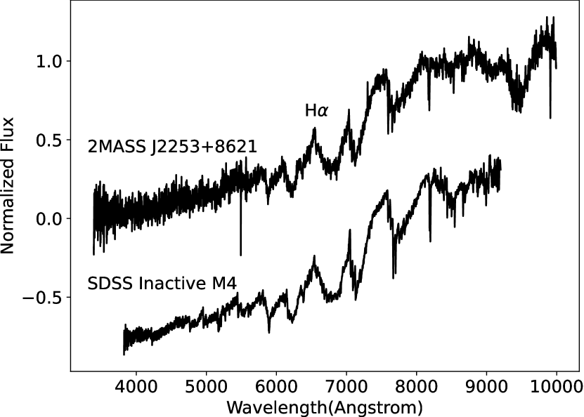
Figure 11: Palomar DBSP spectrum of the M dwarf 2MASS J22535150+8621556 coincident with the radio transient ILT J225347+862146. The location of the 6562  Å H$\alpha$ line is indicated. An SDSS inactive M4 dwarf template spectrum (Bochanski et al., 2007) is plotted with offset for reference. The feature at $7300$ Å was present in other sources during the same night of observation and is thus likely not astrophysical.

Table 6: Basic parameters for the coincident M dwarf

Parameter	Value
2MASS Designation	2MASS J22535150+8621556
Gaia Designation	Gaia EDR3 2301292714713394688
Right Ascension (J2000)	$22^{h}53^{m}51.45^{s}$
Declination (J2000)	$+86^{\circ}21^{\prime}55.56^{\prime\prime}$
Distance	$420^{+18}_{-22}$ pc
Gaia G magnitude	18.8
Gaia Bp-Rp color	2.59
Spectral type	M4V

2MASS (Skrutskie et al., 2006) Gaia EDR 3 (Gaia Collaboration et al., 2021)

Without a detection of another instance of the transient population, we revisit an optical coincidence of the Stewart et al. (2016) transient for clues on the nature of the population. In an attempt to elucidate the nature of ILT J225347+862146, Stewart et al. (2016) obtained a deep ($r^{\prime}\sim 22.5$) image of the field. There was no discernible galaxy in their image. For a galactic origin, Stewart et al. (2016) considered radio flare stars, in particular M dwarfs, as viable progenitors to this population of transients. In their optical image, they found one high-proper-motion objects within the $1\sigma$ localization circle. They concluded that the object did not have colors consistent with an M dwarf, noting however that their color calibration had significant errors.

We cross-matched the $1\sigma$-radius localization region of ILT J225347+862146 with the Gaia (Gaia Collaboration et al., 2016) Early Data Release 3 source catalog (Gaia Collaboration et al., 2021) and found two matches. The closer match, at an offset of $10\arcsec$, is an M dwarf at a distance of $420^{+18}_{-22}$ pc (Bailer-Jones et al., 2021). The M dwarf is indeed the high-proper-motion object identified by Stewart et al. (2016). The farther offset match at $13\arcsec$ is a K dwarf at a distance of $1.7\pm 0.2$ kpc (Bailer-Jones et al., 2021).

In order to prioritize follow-up efforts, we used the procedures outlined below to evaluate the significance of the coincidence and attempted to identify a posteriori bias. We did not seek to claim an association of the star with the transient in this exercise. Rather, we assessed whether the coincidence warranted further investigations into any of these objects. We emphasize that only more instances of the population, or observed peculiarities of the coincident stars that may explain the transient, can lend credence to the association claim of the transient with a stellar source.

For each object, we randomly selected locations in the Stewart et al. (2016) survey field and searched for objects with parallax greater than the $1\sigma$ upper bound of the object within the $1\sigma$ localization radius of $14\arcsec$ and calculated the fraction of trials that resulted in matches. The calculated fraction represented the chance of finding any object within the $14\arcsec$ localization radius with greater parallax than the match in question. We found this chance coincidence probability to be $1.9\%$ for the M dwarf and $15\%$ for the K dwarf. The probability of finding any galactic Gaia source within a $14\arcsec$ radius in the Stewart et al. (2016) field is $16\%$. We used distance as a discriminating factor because bright transients from a nearer source is in general energetically more plausible. The low chance association rate is not due to survey incompleteness for dim sources, because Gaia is $>99\%$ complete down to $G>20$ at this declination (Boubert & Everall, 2020). Although our chance coincidence criteria were quite general, the criteria were determined after the we identified the coincidence. As such, the significance of the coincidence may be inflated. Based on the low chance coincidence rate, we decided to obtain follow-up data on the M dwarf.

We obtained a spectrum of the M dwarf with the Double Spectrograph (DBSP; Oke & Gunn, 1982) on the 200-inch Hale telescope. The spectrum is consistent with an inactive M4 dwarf, exhibiting no excess H$\alpha$ emission nor signs of a companion. The Gaia (Gaia Collaboration et al., 2021), Wide-field Infrared Survey Explorer (WISE; Wright et al., 2010), and Two Micron All Sky Survey (2MASS Skrutskie et al., 2006) colors are consistent with a main sequence M4 dwarf. Table 6 summarizes the basic properties of the M dwarf. We searched for signs of variability in other wavelengths. The M dwarf was marginally detected in the Transiting Exoplanet Survey Satellite (TESS; Ricker et al., 2015) Full Frame Images (FFIs) for sectors 18, 19, 20 as well as Zwicky Transient Facility (ZTF; Masci et al., 2019) Data Release 6, and not detected in Monitor of All-sky X-ray Image (MAXI; Matsuoka et al., 2009). The light curves from TESS, ZTF, or MAXI did not show any transient behavior, with the caveat of low signal-to-noise ratios.

If the M dwarf was responsible for the transient, the implied peak isotropic spectral luminosity $L_{\nu}\sim 3\times 10^{21}$ erg Hz^-1s^-1. The peak luminosity of the transient, assuming that the emission is broadband, is $\nu L_{\nu}\sim 2\times 10^{29}$ erg s^-1. The peak luminosity and the peak spectral luminosity would be many orders of magnitude higher than those of the brightest bursts ever seen from stars at centimeter to decameter wavelengths (e.g. Spangler & Moffett, 1976; Osten & Bastian, 2008, although they were both targeted observations). Given the lack of observed peculiarity of the M dwarf, we are unable to ascertain its association with the transient.

7 Conclusion

We presented results from a $137$ hr transient survey with the OVRO-LWA. We designed the survey to search in a narrow bandwidth, in a much greater sky area, and with enough sensitivity to detect events like the low-frequency transient ILT J225347+862146 discovered by Stewart et al. (2016). We also presented an M dwarf coincident with this transient and optical follow-up observations. This work represents the most targeted effort to date to elucidate the nature of the population underlying this transient. The main findings of this work are as follows:

1. We adopted a Bayesian inference and model comparison approach to model and compare transient surveys. Our Bayesian approach accounts for our widely varying sensitivity as a function of FOV and different transient population properties. It can be extended readily to model the nuances of each transient survey.

2. Despite searching for almost two orders of magnitude larger total sky area, our narrowband transient search yielded no detections. One possible explanation for our non-detection and the non-detection of the Anderson et al. (2019) broadband search is that Stewart et al. (2016) detected an extreme sample of the fluence distribution (i.e. discovery bias). In this scenario, we revised the surface density of transients like ILT J225347+862146 to $1.1\times 10^{-7}\deg^{-2}$, a factor of 30 lower than the estimate implied by the Stewart et al. (2016) detection. The $95\%$ credible interval of the surface density is $(3.5\times 10^{-12},3.4\times 10^{-7})\deg^{-2}$,

3. The alternative explanation is that the population produces transients that are clustered in time with very low duty cycles and low all-sky source density. Therefore, compared to the $4$ month time baseline of Stewart et al. (2016), our short time baseline ($5$ days) was responsible for our non-detection. Because our much larger FOV compared to Stewart et al. (2016), the allowed parameter space for this hypothesis is small. However, the cost for testing this hypothesis is relatively low.

4. Owing to the availability of the Gaia catalog, we identified an object within the $1\sigma$ localization region of ILT J225347+862146 as an M dwarf at $420$ pc, with an a posteriori chance coincidence rate $<2\%$. However, we are unable to robustly associate this M dwarf with the transient based on follow-up spectroscopy and existing catalog data.

Appendix A Derivation of an Uninformative Prior

When surveys contain very few detections, the choice of prior can impact the results of the inference quite significantly. Here we derive a prior on our model parameters that is less informative than a uniform prior. We write our model in simplified notations as

$$\lambda=\rho_{*}S^{-\gamma},$$ (A1)

where $\lambda/\Omega_{tot}\rightarrow\lambda$, $S/S_{*}\rightarrow S$ when compared to Eq. 3. We seek to derive a prior distribution density function $p(\rho_{*},\gamma)$ that is invariant under reasonable reparameterization, such that it does not encode information based on the parameterization of the problem. Here we follow Jeffreys (1946) and VanderPlas (2014) and derive one such prior using the symmetry of the model under exchange of variables. Since $S$ and $\lambda$ are symmetric in this relationship, the model can also be rewritten as

$$S=\rho_{*}^{\prime}\lambda^{-\gamma^{\prime}},$$ (A2)

i.e. a model of typical flux density changing with occurrence rate. We can solve for the transformation $\rho_{*}^{\prime}=\rho_{*}^{1/\gamma}$ and $\gamma^{\prime}=1/\gamma$.

The prior density function transforms as follows

$$p(\rho_{*},\gamma)d\rho_{*}d\gamma=q(\rho_{*}^{\prime},\gamma^{\prime})d\rho_{*}^{\prime}d\gamma^{\prime},$$ (A3)

where $q(\rho_{*}^{\prime},\gamma^{\prime})$ is the prior density function on the reparameterized parameters. Because we claim the same ignorance whether we parameterize the problem with $(\rho_{*},\gamma)$ or $(\rho_{*}^{\prime},\gamma^{\prime})$, the prior distribution function on the two parameterization must be the same:

$$p(\rho_{*},\gamma_{*})=q(\rho_{*}^{\prime},\gamma^{\prime}).$$ (A4)

The determinant of the Jacobian matrix of the transformation $(\rho_{*},\gamma)\rightarrow(\rho_{*}^{\prime},\gamma^{\prime})$ is $-\rho^{\frac{1}{\gamma}-1}/\gamma^{3}$.

The change of variable theorem then gives

$$p(\rho_{*},\gamma)d\rho_{*}d\gamma=\left|-\frac{\rho^{\frac{1}{\gamma}-1}}{\gamma^{3}}\right|p(\rho_{*}^{1/\gamma},1/\gamma)d\rho_{*}d\gamma.$$ (A5)

Imposing that the $\rho_{*}$ and $\gamma$ are independent in our prior, a functional form that satisfies the above requirement is

$$p(\rho_{*})\propto 1/\rho_{*},$$ (A6)

$$p(\gamma)\propto\gamma^{-3/2}.$$ (A7)

When we modify $\rho$ to $r\rho$ in the two-population model $\mathcal{M}_{2}$ (Eq. 4.2.4), Eq. A6 is satisfied when $p(r)\propto 1/r$. This prior density is also invariant under the reparameterization $r\rightarrow 1/r$.

References

- Anderson et al. (2018) Anderson, M. M., Hallinan, G., Eastwood, M. W., et al. 2018, ApJ, 864, 22, doi: 10.3847/1538-4357/aad2d7
- Anderson et al. (2019) —. 2019, ApJ, 886, 123, doi: 10.3847/1538-4357/ab4f87
- Astropy Collaboration et al. (2018) Astropy Collaboration, Price-Whelan, A. M., Sipőcz, B. M., et al. 2018, AJ, 156, 123, doi: 10.3847/1538-3881/aabc4f
- Bailer-Jones et al. (2021) Bailer-Jones, C. A. L., Rybizki, J., Fouesneau, M., Demleitner, M., & Andrae, R. 2021, AJ, 161, 147, doi: 10.3847/1538-3881/abd806
- Bates et al. (2014) Bates, S. D., Lorimer, D. R., Rane, A., & Swiggum, J. 2014, MNRAS, 439, 2893, doi: 10.1093/mnras/stu157
- Bell et al. (2014) Bell, M. E., Murphy, T., Kaplan, D. L., et al. 2014, MNRAS, 438, 352, doi: 10.1093/mnras/stt2200
- Bellm & Sesar (2016) Bellm, E. C., & Sesar, B. 2016, pyraf-dbsp: Reduction pipeline for the Palomar Double Beam Spectrograph. http://ascl.net/1602.002
- Bochanski et al. (2007) Bochanski, J. J., West, A. A., Hawley, S. L., & Covey, K. R. 2007, AJ, 133, 531, doi: 10.1086/510240
- Boubert & Everall (2020) Boubert, D., & Everall, A. 2020, MNRAS, 497, 4246, doi: 10.1093/mnras/staa2305
- Callingham et al. (2021) Callingham, J. R., Pope, B. J. S., Feinstein, A. D., et al. 2021, A&A, 648, A13, doi: 10.1051/0004-6361/202039144
- Carbone et al. (2017) Carbone, D., van der Horst, A. J., Wijers, R. A. M. J., & Rowlinson, A. 2017, MNRAS, 465, 4106, doi: 10.1093/mnras/stw3013
- Carbone et al. (2016) Carbone, D., van der Horst, A. J., Wijers, R. A. M. J., et al. 2016, MNRAS, 459, 3161, doi: 10.1093/mnras/stw539
- Cendes et al. (2014) Cendes, Y., Wijers, R. A. M. J., Swinbank, J. D., et al. 2014, arXiv e-prints, arXiv:1412.3986. https://arxiv.org/abs/1412.3986
- Ching & Chen (2007) Ching, J., & Chen, Y.-C. 2007, Journal of Engineering Mechanics, 133, 816, doi: 10.1061/(ASCE)0733-9399(2007)133:7(816)
- Clark et al. (2013) Clark, M. A., LaPlante, P. C., & Greenhill, L. J. 2013, International Journal of High Performance Computing Applications, 27, 178, doi: 10.1177/1094342012444794
- Cohen (2004) Cohen, A. 2004, Estimates of the Classical Confusion Limit for the LWA, Long Wavelength Array (LWA) Memo Series 17, Naval Research Laboratory. https://www.faculty.ece.vt.edu/swe/lwa/memo/lwa0017.pdf
- Davidson et al. (2020) Davidson, D. B., Bolli, P., Bercigli, M., et al. 2020, in 2020 XXXIIIrd General Assembly and Scientific Symposium of the International Union of Radio Science, 1–4, doi: 10.23919/URSIGASS49373.2020.9232307
- de Ruiter et al. (2021) de Ruiter, I., Leseigneur, G., Rowlinson, A., et al. 2021, MNRAS, 508, 2412, doi: 10.1093/mnras/stab2695
- Dewdney et al. (2009) Dewdney, P. E., Hall, P. J., Schilizzi, R. T., & Lazio, T. J. L. W. 2009, IEEE Proceedings, 97, 1482, doi: 10.1109/JPROC.2009.2021005
- Duane et al. (1987) Duane, S., Kennedy, A., Pendleton, B. J., & Roweth, D. 1987, Physics Letters B, 195, 216, doi: https://doi.org/10.1016/0370-2693(87)91197-X
- Eastwood (2016) Eastwood, M. W. 2016, TTCal, 0.3.0, Zenodo, doi: 10.5281/zenodo.1049160
- Eastwood et al. (2018) Eastwood, M. W., Anderson, M. M., Monroe, R. M., et al. 2018, AJ, 156, 32, doi: 10.3847/1538-3881/aac721
- Ellingson et al. (2013) Ellingson, S. W., Taylor, G. B., Craig, J., et al. 2013, IEEE Transactions on Antennas and Propagation, 61, 2540, doi: 10.1109/TAP.2013.2242826
- Feng et al. (2017) Feng, L., Vaulin, R., Hewitt, J. N., et al. 2017, AJ, 153, 98, doi: 10.3847/1538-3881/153/3/98
- Frail et al. (2012) Frail, D. A., Kulkarni, S. R., Ofek, E. O., Bower, G. C., & Nakar, E. 2012, ApJ, 747, 70, doi: 10.1088/0004-637X/747/1/70
- Gaia Collaboration et al. (2016) Gaia Collaboration, Prusti, T., de Bruijne, J. H. J., et al. 2016, A&A, 595, A1, doi: 10.1051/0004-6361/201629272
- Gaia Collaboration et al. (2021) Gaia Collaboration, Smart, R. L., Sarro, L. M., et al. 2021, A&A, 649, A6, doi: 10.1051/0004-6361/202039498
- Gardenier et al. (2019) Gardenier, D. W., van Leeuwen, J., Connor, L., & Petroff, E. 2019, A&A, 632, A125, doi: 10.1051/0004-6361/201936404
- Gehrels (1986) Gehrels, N. 1986, ApJ, 303, 336, doi: 10.1086/164079
- Hajela et al. (2019) Hajela, A., Mooley, K. P., Intema, H. T., & Frail, D. A. 2019, MNRAS, 490, 4898, doi: 10.1093/mnras/stz2918
- Hickish et al. (2016) Hickish, J., Abdurashidova, Z., Ali, Z., et al. 2016, Journal of Astronomical Instrumentation, 5, 1641001, doi: 10.1142/S2251171716410014
- Hoffman et al. (2014) Hoffman, M. D., Gelman, A., et al. 2014, J. Mach. Learn. Res., 15, 1593
- Hunter (2007) Hunter, J. D. 2007, Computing in Science & Engineering, 9, 90, doi: 10.1109/MCSE.2007.55
- Hurley-Walker & Hancock (2018) Hurley-Walker, N., & Hancock, P. J. 2018, Astronomy and Computing, 25, 94, doi: 10.1016/j.ascom.2018.08.006
- Hyman et al. (2002) Hyman, S. D., Lazio, T. J. W., Kassim, N. E., & Bartleson, A. L. 2002, AJ, 123, 1497, doi: 10.1086/338905
- Hyman et al. (2005) Hyman, S. D., Lazio, T. J. W., Kassim, N. E., et al. 2005, Nature, 434, 50, doi: 10.1038/nature03400
- Hyman et al. (2009) Hyman, S. D., Wijnands, R., Lazio, T. J. W., et al. 2009, ApJ, 696, 280, doi: 10.1088/0004-637X/696/1/280
- Jaeger et al. (2012) Jaeger, T. R., Hyman, S. D., Kassim, N. E., & Lazio, T. J. W. 2012, AJ, 143, 96, doi: 10.1088/0004-6256/143/4/96
- Jankowski et al. (2018) Jankowski, F., van Straten, W., Keane, E. F., et al. 2018, MNRAS, 473, 4436, doi: 10.1093/mnras/stx2476
- Jeffreys (1946) Jeffreys, H. 1946, Proceedings of the Royal Society of London. Series A. Mathematical and Physical Sciences, 186, 453, doi: 10.1098/rspa.1946.0056
- Kamary et al. (2014) Kamary, K., Mengersen, K., Robert, C. P., & Rousseau, J. 2014, arXiv e-prints, arXiv:1412.2044. https://arxiv.org/abs/1412.2044
- Kass & Raftery (1995) Kass, R. E., & Raftery, A. E. 1995, Journal of the American Statistical Association, 90, 773, doi: 10.1080/01621459.1995.10476572
- Kassim et al. (2007) Kassim, N. E., Lazio, T. J. W., Erickson, W. C., et al. 2007, ApJS, 172, 686, doi: 10.1086/519022
- Kipping (2021) Kipping, D. 2021, MNRAS, 504, 4054, doi: 10.1093/mnras/stab1129
- Kluyver et al. (2016) Kluyver, T., Ragan-Kelley, B., Pérez, F., et al. 2016, in Positioning and Power in Academic Publishing: Players, Agents and Agendas, ed. F. Loizides & B. Scmidt (IOS Press), 87–90. https://eprints.soton.ac.uk/403913/
- Kocz et al. (2015) Kocz, J., Greenhill, L. J., Barsdell, B. R., et al. 2015, Journal of Astronomical Instrumentation, 4, 1550003, doi: 10.1142/S2251171715500038
- Kuiack et al. (2021a) Kuiack, M., Wijers, R. A. M. J., Shulevski, A., et al. 2021a, MNRAS, 505, 2966, doi: 10.1093/mnras/stab1504
- Kuiack et al. (2021b) Kuiack, M. J., Wijers, R. A. M. J., Shulevski, A., & Rowlinson, A. 2021b, MNRAS, 504, 4706, doi: 10.1093/mnras/stab1156
- Kumar et al. (2021) Kumar, P., Shannon, R. M., Flynn, C., et al. 2021, MNRAS, 500, 2525, doi: 10.1093/mnras/staa3436
- Kumar et al. (2019) Kumar, R., Carroll, C., Hartikainen, A., & Martin, O. 2019, Journal of Open Source Software, 4, 1143, doi: 10.21105/joss.01143
- Lazio et al. (2010) Lazio, T. J. W., Clarke, T. E., Lane, W. M., et al. 2010, AJ, 140, 1995, doi: 10.1088/0004-6256/140/6/1995
- Lightkurve Collaboration et al. (2018) Lightkurve Collaboration, Cardoso, J. V. d. M., Hedges, C., et al. 2018, Lightkurve: Kepler and TESS time series analysis in Python, Astrophysics Source Code Library. http://ascl.net/1812.013
- Lorimer et al. (2007) Lorimer, D. R., Bailes, M., McLaughlin, M. A., Narkevic, D. J., & Crawford, F. 2007, Science, 318, 777, doi: 10.1126/science.1147532
- Macquart (2014) Macquart, J.-P. 2014, PASA, 31, e031, doi: 10.1017/pasa.2014.27
- Macquart & Ekers (2018) Macquart, J. P., & Ekers, R. D. 2018, MNRAS, 474, 1900, doi: 10.1093/mnras/stx2825
- Masci et al. (2019) Masci, F. J., Laher, R. R., Rusholme, B., et al. 2019, PASP, 131, 018003, doi: 10.1088/1538-3873/aae8ac
- Matsuoka et al. (2009) Matsuoka, M., Kawasaki, K., Ueno, S., et al. 2009, PASJ, 61, 999, doi: 10.1093/pasj/61.5.999
- McMullin et al. (2007) McMullin, J. P., Waters, B., Schiebel, D., Young, W., & Golap, K. 2007, in Astronomical Society of the Pacific Conference Series, Vol. 376, Astronomical Data Analysis Software and Systems XVI, ed. R. A. Shaw, F. Hill, & D. J. Bell, 127
- Melrose (2017) Melrose, D. B. 2017, Reviews of Modern Plasma Physics, 1, 5, doi: 10.1007/s41614-017-0007-0
- Metzger et al. (2015) Metzger, B. D., Williams, P. K. G., & Berger, E. 2015, The Astrophysical Journal, 806, 224, doi: 10.1088/0004-637X/806/2/224
- Minson et al. (2013) Minson, S. E., Simons, M., & Beck, J. L. 2013, Geophysical Journal International, 194, 1701, doi: 10.1093/gji/ggt180
- Murphy et al. (2017) Murphy, T., Kaplan, D. L., Croft, S., et al. 2017, MNRAS, 466, 1944, doi: 10.1093/mnras/stw3087
- Noordam (2004) Noordam, J. E. 2004, in Society of Photo-Optical Instrumentation Engineers (SPIE) Conference Series, Vol. 5489, Ground-based Telescopes, ed. J. Oschmann, Jacobus M., 817–825, doi: 10.1117/12.544262
- Obenberger et al. (2015) Obenberger, K. S., Taylor, G. B., Hartman, J. M., et al. 2015, Journal of Astronomical Instrumentation, 4, 1550004, doi: 10.1142/S225117171550004X
- Offringa et al. (2012) Offringa, A. R., van de Gronde, J. J., & Roerdink, J. B. T. M. 2012, A&A, 539, A95, doi: 10.1051/0004-6361/201118497
- Offringa et al. (2013a) Offringa, A. R., de Bruyn, A. G., Zaroubi, S., et al. 2013a, MNRAS, 435, 584, doi: 10.1093/mnras/stt1337
- Offringa et al. (2013b) —. 2013b, A&A, 549, A11, doi: 10.1051/0004-6361/201220293
- Offringa et al. (2014) Offringa, A. R., McKinley, B., Hurley-Walker, N., et al. 2014, MNRAS, 444, 606, doi: 10.1093/mnras/stu1368
- Oke & Gunn (1982) Oke, J. B., & Gunn, J. E. 1982, PASP, 94, 586, doi: 10.1086/131027
- Osten & Bastian (2008) Osten, R. A., & Bastian, T. S. 2008, ApJ, 674, 1078, doi: 10.1086/525013
- Perley (2002) Perley, R. 2002, Attenuation of Radio Frequency Interference by Interferometric Fringe Rotation, VLA Expansion Project Memo 49, National Radio Astronomy Observatory. https://library.nrao.edu/public/memos/evla/EVLAM_49.pdf
- Pleunis et al. (2021) Pleunis, Z., Michilli, D., Bassa, C. G., et al. 2021, ApJ, 911, L3, doi: 10.3847/2041-8213/abec72
- Polisensky et al. (2016) Polisensky, E., Lane, W. M., Hyman, S. D., et al. 2016, ApJ, 832, 60, doi: 10.3847/0004-637X/832/1/60
- Prasad et al. (2016) Prasad, P., Huizinga, F., Kooistra, E., et al. 2016, Journal of Astronomical Instrumentation, 5, 1641008, doi: 10.1142/S2251171716410087
- Raba et al. (2020) Raba, R., Schiebel, D., Emonts, B., et al. 2020, in Astronomical Society of the Pacific Conference Series, Vol. 527, Astronomical Society of the Pacific Conference Series, ed. R. Pizzo, E. R. Deul, J. D. Mol, J. de Plaa, & H. Verkouter, 271. https://arxiv.org/abs/1912.09439
- Reiss (2016) Reiss, D. J. 2016, DMTN-007: Dipole characterization for image differencing. https://dmtn-007.lsst.io/
- Ricker et al. (2015) Ricker, G. R., Winn, J. N., Vanderspek, R., et al. 2015, Journal of Astronomical Telescopes, Instruments, and Systems, 1, 014003, doi: 10.1117/1.JATIS.1.1.014003
- Rowlinson et al. (2016) Rowlinson, A., Bell, M. E., Murphy, T., et al. 2016, MNRAS, 458, 3506, doi: 10.1093/mnras/stw451
- Ruhe et al. (2021) Ruhe, D., Kuiack, M., Rowlinson, A., Wijers, R., & Forré, P. 2021, arXiv e-prints, arXiv:2103.15418. https://arxiv.org/abs/2103.15418
- Salvatier et al. (2016) Salvatier, J., Wiecki, T. V., & Fonnesbeck, C. 2016, PeerJ Computer Science, 2, e55
- Salvini & Wijnholds (2014) Salvini, S., & Wijnholds, S. J. 2014, A&A, 571, A97, doi: 10.1051/0004-6361/201424487
- Shannon et al. (2018) Shannon, R. M., Macquart, J. P., Bannister, K. W., et al. 2018, Nature, 562, 386, doi: 10.1038/s41586-018-0588-y
- Skrutskie et al. (2006) Skrutskie, M. F., Cutri, R. M., Stiening, R., et al. 2006, AJ, 131, 1163, doi: 10.1086/498708
- Smirnov & Tasse (2015) Smirnov, O. M., & Tasse, C. 2015, MNRAS, 449, 2668, doi: 10.1093/mnras/stv418
- Sokolowski et al. (2021) Sokolowski, M., Wayth, R. B., Bhat, N. D. R., et al. 2021, PASA, 38, e023, doi: 10.1017/pasa.2021.16
- Spangler & Moffett (1976) Spangler, S. R., & Moffett, T. J. 1976, ApJ, 203, 497, doi: 10.1086/154105
- Stewart et al. (2016) Stewart, A. J., Fender, R. P., Broderick, J. W., et al. 2016, MNRAS, 456, 2321, doi: 10.1093/mnras/stv2797
- Sullivan et al. (2012) Sullivan, I. S., Morales, M. F., Hazelton, B. J., et al. 2012, ApJ, 759, 17, doi: 10.1088/0004-637X/759/1/17
- Tasse et al. (2018) Tasse, C., Hugo, B., Mirmont, M., et al. 2018, A&A, 611, A87, doi: 10.1051/0004-6361/201731474
- Taylor et al. (2012) Taylor, G. B., Ellingson, S. W., Kassim, N. E., et al. 2012, Journal of Astronomical Instrumentation, 1, 1250004, doi: 10.1142/S2251171712500043
- Tingay et al. (2013) Tingay, S. J., Goeke, R., Bowman, J. D., et al. 2013, PASA, 30, e007, doi: 10.1017/pasa.2012.007
- Treumann (2006) Treumann, R. A. 2006, A&A Rev., 13, 229, doi: 10.1007/s00159-006-0001-y
- Trott et al. (2013) Trott, C. M., Tingay, S. J., Wayth, R. B., et al. 2013, ApJ, 767, 4, doi: 10.1088/0004-637X/767/1/4
- van Haarlem et al. (2013) van Haarlem, M. P., Wise, M. W., Gunst, A. W., et al. 2013, A&A, 556, A2, doi: 10.1051/0004-6361/201220873
- VanderPlas (2014) VanderPlas, J. 2014, arXiv e-prints, arXiv:1411.5018. https://arxiv.org/abs/1411.5018
- Varghese et al. (2019) Varghese, S. S., Obenberger, K. S., Dowell, J., & Taylor, G. B. 2019, ApJ, 874, 151, doi: 10.3847/1538-4357/ab07c6
- Vedantham et al. (2014) Vedantham, H. K., Koopmans, L. V. E., de Bruyn, A. G., et al. 2014, MNRAS, 437, 1056, doi: 10.1093/mnras/stt1878
- Veenboer & Romein (2020) Veenboer, B., & Romein, J. W. 2020, Astronomy and Computing, 32, 100386, doi: 10.1016/j.ascom.2020.100386
- Vehtari et al. (2015) Vehtari, A., Gelman, A., & Gabry, J. 2015, arXiv e-prints, arXiv:1507.04544. https://arxiv.org/abs/1507.04544
- Vehtari et al. (2021) Vehtari, A., Gelman, A., Simpson, D., Carpenter, B., & Bürkner, P.-C. 2021, Bayesian Analysis, 16, 667 , doi: 10.1214/20-BA1221
- Virtanen et al. (2020) Virtanen, P., Gommers, R., Oliphant, T. E., et al. 2020, Nature Methods, doi: https://doi.org/10.1038/s41592-019-0686-2
- Waskom (2021) Waskom, M. L. 2021, Journal of Open Source Software, 6, 3021, doi: 10.21105/joss.03021
- Watanabe (2013) Watanabe, S. 2013, Journal of Machine Learning Research, 14, 867
- Wayth et al. (2017) Wayth, R., Sokolowski, M., Booler, T., et al. 2017, PASA, 34, e034, doi: 10.1017/pasa.2017.27
- Wayth et al. (2018) Wayth, R. B., Tingay, S. J., Trott, C. M., et al. 2018, PASA, 35, e033, doi: 10.1017/pasa.2018.37
- Wilensky et al. (2019) Wilensky, M. J., Morales, M. F., Hazelton, B. J., et al. 2019, PASP, 131, 114507, doi: 10.1088/1538-3873/ab3cad
- Wright et al. (2010) Wright, E. L., Eisenhardt, P. R. M., Mainzer, A. K., et al. 2010, AJ, 140, 1868, doi: 10.1088/0004-6256/140/6/1868