On the geometry of the orthogonal momentum amplituhedron

Abstract

In this paper we study the orthogonal momentum amplituhedron $\mathcal{O}_{k}$, a recently introduced positive geometry that encodes the tree-level scattering amplitudes in ABJM theory. We generate the full boundary stratification of $\mathcal{O}_{k}$ and show that its boundaries can be labelled by so-called orthogonal Grassmannian forests (OG forests). We also determine the generating function for enumerating boundaries according to their dimension and show that the Euler characteristic of $\mathcal{O}_{k}$ equals one. This provides a strong indication that the orthogonal momentum amplituhedron is homeomorphic to a ball. This paper is supplemented with the Mathematica package orthitroids which contains useful functions for studying the positive orthogonal Grassmannian and the orthogonal momentum amplituhedron.

1 Introduction

In recent years we have seen tremendous interest in positive geometries Arkani-Hamed:2017tmz that encode observables in quantum field theories, and in particular the ones that can be employed to study scattering amplitudes. A particularly fruitful theory where positive geometries can be defined is $\mathcal{N}=4$ super Yang-Mills, where the amplituhedron $\mathcal{A}_{n,k}$ Arkani-Hamed:2013jha and the momentum amplituhedron $\mathcal{M}_{n,k}$ Damgaard:2019ztj have been introduced to encode the tree-level scattering amplitudes. Both of these geometries are defined as the image of the positive Grassmannian through a linear map. More recently, a similar construction has been proposed for ABJM theory tree-level scattering amplitudes Huang:2021jlh ; He:2021llb using the orthogonal Grassmannian and its positive part. The resulting geometry, denoted as $\mathcal{O}_{k}$ in this paper, is $(2k-3)$-dimensional and can be thought of as a deformation of the ABHY associahedron $A_{2k-3}$ Arkani-Hamed:2017mur where faces corresponding to even-particle planar Mandelstam variables are squashed to lower dimensional boundaries.

In this paper we study properties of $\mathcal{O}_{k}$, and in particular provide a complete classification of its boundaries. To this end we use the algorithm developed in Lukowski:2019kqi where it was successfully applied to find all boundaries of the amplituhedron $\mathcal{A}_{n,k}^{(2)}$, and which has been subsequently used to find all boundaries of the momentum amplituhedron $\mathcal{M}_{n,k}$ in Lukowski:2020bya . Applying this algorithm to the orthogonal momentum amplituhedron $\mathcal{O}_{k}$, we observe that all boundaries can be labelled by a particular class of graphs, which we call orthogonal Grassmannian forests, that correspond to all possible factorizations of ABJM amplitudes. This observation is analogous to the one that has been made for $\mathcal{N}=4$ sYM in Lukowski:2020bya , where the boundaries of the momentum amplihedron $\mathcal{M}_{n,k}$ can be labelled using Grassmannian forests, see Moerman:2021cjg . Both form a subset of the Grassmannian graphs introduced in Postnikov:2018jfq . In this paper we summarise our explorations of the boundaries for $\mathcal{O}_{k}$ for $k\leq 7$, and provide a conjecture on the boundary stratification for all $k$. In particular, using the methods developed in Moerman:2021cjg , we provide a generating function for the number of boundaries of a given dimension and this allows us to show that the Euler characteristic for the orthogonal momentum amplituhedron equals one. This story parallels the one developed for the momentum amplituhedron.

Moreover, it has been shown in He:2021llb that both the interior of the ABHY associahedron $A_{2k-3}$ and the interior of the orthogonal momentum amplituhedron $\mathcal{O}_{k}$ are diffeomorphic to the positive part of the moduli space of $n$ points on the Riemann sphere and therefore are diffeomorphic to each other. This is however not true for their closures. Nevertheless, in this paper we show that there is a simple diagrammatic way to understand how the boundaries of the associahedron naturally reduce to the boundaries of the orthogonal momentum amplituhedron.

This paper is organised as follows. In Section 2 we recall the definition of the positive orthogonal Grassmannian and collect its basic properties. In Section 3 we define the orthogonal momentum amplituhedron following He:2021llb ; Huang:2021jlh and find its boundary stratification. Then, in Section 4 we discuss the generating function for the number of boundaries of $\mathcal{O}_{k}$. Section 5 provides details on the diagrammatic map from boundaries of the associahedron $A_{2k-3}$ to those of the orthogonal momentum amplituhedron $\mathcal{O}_{k}$. We provide details on the Mathematica package orthitroids in Appendix A.

2 Positive Orthogonal Grassmannian

Let us start by recalling a few basic facts about Grassmannian spaces and their positive parts. The real Grassmannian $G(k,n)$ is the space of $k$-dimensional linear subspaces of $\mathbb{R}^{n}$. Elements of $G(k,n)$ can be represented by $k\times n$ matrices of maximal rank, where matrices related by $\mathrm{GL}(k)$ transformations are identified. The positive Grassmannian $G_{+}(k,n)$, extensively studied by Postnikov in Postnikov:2006kva , is defined as the subset of matrices $C\in G(k,n)$ for which all ordered maximal minors are non-negative. The boundary stratification of the positive Grassmannian $G_{+}(k,n)$ is well known Postnikov:2006kva and it can be described in terms of positroid cells. Positroid cells of $G_{+}(k,n)$ are in a bijection with various combinatorial objects, including decorated permutations of type $(k,n)$, i.e. permutations on $[n]=\{1,\ldots,n\}$ with $k$ anti-exceedances where fixed points are coloured either black or white, equivalence classes of reduced plabic (planar bicoloured) graphs, and, more generally, equivalence classes of reduced Grassmannian graphs Postnikov:2018jfq .

In this paper we will be interested in an equivalent description of (a particular analytic continuation of) the positive orthogonal Grassmannian $OG_{+}(k)$ introduced in Huang:2013owa . This is defined as a $\frac{k(k-1)}{2}$-dimensional slice of the positive Grassmannian $G_{+}(k,2k)$ satisfying certain orthogonality conditions:

$$OG_{+}(k)=\left\{C\in G_{+}(k,2k):C\cdot\eta\cdot C^{T}=0\right\}\,,$$ (1)

where $\eta\coloneqq\mathrm{diag}(-,+,-,\cdots,+)$. Similar to the positive Grassmannian, the boundary stratification of the positive orthogonal Grassmannian $OG_{+}(k)$ was given in Kim:2014hva in terms of cells which we call orthitroid cells. Orthitroid cells of $OG_{+}(k)$ are similarly in a bijection with various combinatorial objects, including permutations on $[2k]$ given as the product of $k$ disjoint two-cycles, a special class of marked Young diagrams called folded OG tableaux Kim:2014hva , and equivalence classes of reduced orthogonal Grassmannian graphs. A permutation on $[2k]$ given as the product of $k$ disjoint two-cycles can be naturally depicted as a crossing diagram as generated by the function oposPermToCrossing; see Figure 1 (left) for an example. For a precise definition of folded OG tableaux, we refer the reader to Section 4.1 of Kim:2014hva . The folded OG tableau of an orthitroid cell can be generated using the function oposPermToYoungReducedNice; see Figure 1 (right) for an example. Our primary interest, however, is in orthogonal Grassmannian graphs.

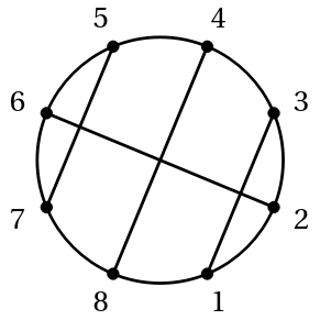
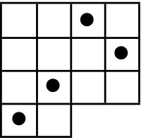
Figure 1: A crossing diagram (left) and folded OG tableau (right) for the permutation $(1\,3)(2\,6)(4\,8)(5\,7)$.

We define an orthogonal Grassmannian graph or OG graph of type $\underline{k}$ to be a finite planar graph $\Gamma$ with vertices $\mathcal{V}(\Gamma)$ and edges $\mathcal{E}(\Gamma)$, embedded in a disk, with $2k$ boundary vertices $\mathcal{V}_{\text{ext}}(\Gamma)=\{b_{1},\ldots,b_{2k}\}$ of degree $1$ on the boundary of the disk labelled counterclockwise. Moreover, all internal vertices $\mathcal{V}_{\text{int}}(\Gamma)=\mathcal{V}(\Gamma)\setminus\mathcal{V}_{\text{ext}}(\Gamma)$ must be connected to the boundary of the disk via a path in $\Gamma$ and have an even degree larger than $2$. We denote by $\mathcal{E}_{\text{int}}(\Gamma)$ the set of internal edges in $\Gamma$, i.e. those which are not adjacent to boundary vertices, and by $\Gamma_{\text{int}}$ the internal subgraph of $\Gamma$. In this paper we are primarily interested in OG graphs which are forests, i.e. have no internal cycles. We define them in analogy with Grassmannian forests defined in Moerman:2021cjg . An orthogonal Grassmannian forest or OG forest is an acyclic OG graph and an orthogonal Grassmannian tree or OG tree is a connected acyclic OG graph. Given an OG forest $\Gamma$ we denote the set of OG trees in $\Gamma$ by $\text{Trees}(\Gamma)$.

To each OG graph $\Gamma$, we can naturally assign a permutation in the following way: one can define a one-way strand $\sigma_{\Gamma}$ which is a directed walk along edges of $\Gamma$ which starts and ends at some boundary vertices. It is defined according to the rules-of-the-road as given in Postnikov:2018jfq . For each vertex $v\in\mathcal{V}_{\text{int}}(\Gamma)$ with adjacent edges labelled clockwise $e_{1},\ldots,e_{d}$, where $d=\deg(v)$, if $\sigma_{\Gamma}$ enters $v$ through edge $e_{i}$, it leaves through edge $e_{j}$, where $j=i+d/2$ (mod $d$). Said differently, if $v$ is thought of as a roundabout with $d=\deg(v)$ exits, $\sigma_{\Gamma}$ always exits the roundabout along the edge directly opposite the one it entered on. An OG graph $\Gamma$ is said to be reduced if

1. There are no strands forming closed loops in $\Gamma_{\text{int}}$.

2. All strands in $\Gamma$ are simple curves without self-intersections.

3. Any pair of strands $\alpha\neq\beta$ cannot have a bad double crossing where there is a pair of vertices $u\neq v$ such that both $\alpha$ and $\beta$ pass from $u$ to $v$; one does allow double crossings where $\alpha$ passes from $u$ to $v$ and $\beta$ passes from $v$ to $u$.

Importantly, OG forests are automatically reduced. The strand permutation of a reduced OG graph of type $\underline{k}$ is a permutation $\sigma_{\Gamma}:[2k]\to[2k]$ where $\sigma_{\Gamma}(i)=j$ if the one-way strand which starts at the boundary vertex $b_{i}$ ends at the boundary vertex $b_{j}$. The strand permutation is always a product of $k$ disjoint two-cycles and it is an invariant of a reduced OG graph. There is also a natural equivalence relation for reduced OG graphs: two reduced OG graphs $\Gamma\neq\Gamma^{\prime}$ are said to be equivalent if their strand permutations are the same, i.e. $\sigma_{\Gamma}=\sigma_{\Gamma^{\prime}}$. OG forests, however, are always unique with respect to this equivalence relation. The OG forest corresponding to a permutation on $[2k]$ given as the product of $k$ disjoint two-cycles can be generated using the function omomPermToForest. Figure 2 shows an example of an OG forest with its strand permutation.

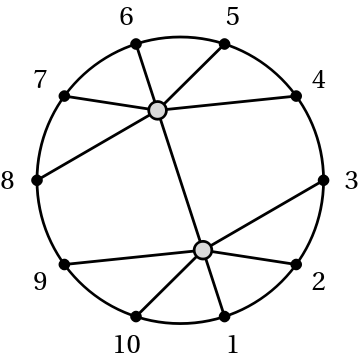
Figure 2: Example of an OG forest of type $\underline{5}$ with strand permutation $(1\,6)(2\,9)(3\,10)(4\,7)(5\,8)$.

As studied in Kim:2014hva , orthitroid cells of $OG_{+}(k)$ are in bijection with permutations $\sigma$ on $[2k]$ given as the product of $k$ disjoint two-cycles, and therefore with equivalence classes of reduced OG graphs $\Gamma$ of type $\underline{k}$. Consequently, these combinatorial objects provide unambiguous labels for orthitroid cells in $OG_{+}(k)$. We denote the orthitroid cell labelled by $\sigma$ (resp., $\Gamma$) as $S_{\sigma}$ (resp., $S_{\Gamma}$). The top cell (i.e. top-dimensional orthitroid cell) of $OG_{+}(k)$ is labelled by the permutation $(1,k+1)(2,k+2)\ldots(k,2k)$.

Each orthitroid cell in $OG_{+}(k)$ can be parametrized using the amalgamation method used in Huang:2013owa , and further explored in Kim:2014hva . In what follows we outline an algorithm, implemented in the function oposPermToMat, for constructing an orthogonal and positive matrix $C(\sigma)$ parametrising the orthitroid cell $S_{\sigma}$. This algorithm closely follows the BCFW construction given in Kim:2014hva with some minor modifications.

Let $\sigma=(i_{1},j_{1})(i_{2},j_{2})\ldots(i_{k},j_{k})$ with $i_{\ell}<j_{\ell}$ and $i_{1}<i_{2}<\ldots<i_{k}$ be a permutation labelling an orthitroid cell $S_{\sigma}$. The labels $i_{1},\ldots,i_{k}$ (resp., $j_{1},\ldots,j_{k}$) are called the pivots (resp., sinks) of $\sigma$ where $i_{\ell}$ is said to be the pivot corresponding to the sink $j_{\ell}$ in $\sigma$ for each $\ell=1,\ldots,k$. There is a unique zero-dimensional orthitroid cell $S_{\sigma_{0}}$ in the boundary stratification of $S_{\sigma}$ labelled by a permutation $\sigma_{0}$ which has the same pivots as $\sigma$. We call $\sigma_{0}$ the zero-permutation corresponding to $\sigma$ and this can be found using the function oposZeroPerm. The matrix $C(\sigma_{0})$ for $S_{\sigma_{0}}$ is constructed according to the prescription for bottom cells given in Kim:2014hva : $C(\sigma_{0})$ is defined to be a sparse $k\times 2k$ matrix whose only non-zero entries are $C_{\ell i_{\ell}}(\sigma_{0})=1$ and $C_{\ell j_{\ell}}(\sigma_{0})=(-1)^{(j_{\ell}-i_{\ell}-1)/2}$ for pivots $i_{\ell}$ and sinks $j_{\ell}$ of $\sigma_{0}$. By construction, $C(\sigma_{0})$ is real, orthogonal and positive.

More generally, to construct the matrix $C(\sigma)$, we first find a series of transpositions $\tau_{1},\ldots,\tau_{d}$ where $d=\dim(S_{\sigma})$ such that

$$\sigma=\tau_{d}\circ\tau_{d-1}\circ\cdots\circ\tau_{1}\circ\sigma_{0}\,.$$ (2)

These transpositions are obtained using the following recursive algorithm. Assume that we have already found decompositions (2) for all codimension-one boundaries $S_{\sigma^{\prime}}\in\partial S_{\sigma}$. For each such $\sigma^{\prime}$ we can write $\sigma=\tau_{\sigma^{\prime}}\circ\sigma^{\prime}$ where $\tau_{\sigma^{\prime}}=(j_{\sigma^{\prime},1},j_{\sigma^{\prime},2})$ is a transposition that corresponds to a BCFW bridge. To guarantee that the constructed matrix is real we need $j_{\sigma^{\prime},1}+j_{\sigma^{\prime},2}$ to be odd, and furthermore we want to use a BCFW bridge that acts on sinks and not on sources. The latter requirement can be translated into the condition that the line connecting the labels $j_{\sigma^{\prime},1}$ and $j_{\sigma^{\prime},2}$ does not cross any other line in the OG graph associated with $S_{\sigma}$. We have checked that it is always possible to find such a BCFW bridge for all orthitroid cells in $OG_{k}$ for $k\leq 7$. The algorithm described above is demonstrated in Figure 3 for the permutation $(1\,3)(2\,6)(4\,8)(5\,7)$.

Having determined the transpositions in (2), we then construct a BCFW rotation matrix $R(\tau_{m})\in SO(2k,2k)$ for each transposition $\tau_{m}$ according to the prescription given in Kim:2014hva . Here

$$SO(2k,2k)\coloneqq\left\{R\in\mathbb{R}^{2k\times 2k}:R\cdot\eta\cdot R^{T}=\eta\right\}\,.$$ (3)

For each transposition $\tau_{m}=(j_{\ell_{1}},j_{\ell_{2}})$, where $j_{\ell_{1}}<j_{\ell_{2}}$, define $R(\tau_{m})$ to have the non-trivial $2\times 2$ submatrix

$$R_{j_{\ell_{1}}j_{\ell_{1}}}(\tau_{m})=R_{j_{\ell_{2}}j_{\ell_{2}}}(\tau_{m})=\cosh\theta_{m}\,,$$ (4)

$$R_{j_{\ell_{1}}j_{\ell_{2}}}(\tau_{m})=R_{j_{\ell_{2}}j_{\ell_{1}}}(\tau_{m})=(-1)^{(j_{\ell_{2}}-j_{\ell_{1}}-1)/2}\sinh\theta_{m}\,,$$ (5)

and to be the identity matrix everywhere else. It is easy to check that $R(\tau_{m})$ is orthogonal. Our earlier requirement that $j_{\ell_{1}}+j_{\ell_{2}}$ be odd is now justified: it ensures that $R(\tau_{m})$ is real! Finally, the matrix $C(\sigma)$ for $S_{\sigma}$ is constructed as

$$C(\sigma)=C(\sigma_{0})R(\tau_{1})R(\tau_{2})\cdots R(\tau_{d})\,,$$ (6)

and is automatically real and orthogonal.

This algorithm for $C(\sigma)$ is implemented in the function oposPermToMat and we have checked that the matrices are positive when $\theta_{i}$ is positive for up to $k=5$. We believe that this will remain true for higher $k$ as well.

$$\begin{gathered}\includegraphics[scale={0.7}]{Figures/bcfw-step-0}\end{gathered}\xrightarrow{\tau_{3}=(67)}\begin{gathered}\includegraphics[scale={0.7}]{Figures/bcfw-step-1}\end{gathered}\xrightarrow{\tau_{2}=(78)}\begin{gathered}\includegraphics[scale={0.7}]{Figures/bcfw-step-2}\end{gathered}\xrightarrow{\tau_{1}=(38)}\begin{gathered}\includegraphics[scale={0.7}]{Figures/bcfw-step-3}\end{gathered}$$

Figure 3: BCFW construction for writing $\sigma=(1\,3)(2\,6)(4\,8)(5\,7)$ as $\sigma=\tau_{3}\circ\tau_{2}\circ\tau_{1}\circ\sigma_{0}$ where $\sigma_{0}=(1\,8)(2\,3)(4\,7)(5\,6)$.

3 Orthogonal Momentum Amplituhedron and its Boundary Stratification

The orthogonal momentum amplituhedron $\mathcal{O}_{k}$ was recently introduced by the authors of Huang:2021jlh and He:2021llb independently. The canonical form of $\mathcal{O}_{k}$ conjecturally encodes tree-level scattering amplitudes of ABJM theory with reduced supersymmetry in a similar way to how the canonical form of the momentum amplituhedron encodes tree-level scattering amplitudes in $\mathcal{N}=4$ super Yang-Mills theory Damgaard:2019ztj . The orthogonal momentum amplituhedron $\mathcal{O}_{k}$ is defined as the image of the map

$$\widetilde{\Phi}_{\Lambda}\colon OG_{+}(k) \to G(k,k+2)$$ (7)

$$c_{\alpha i} \mapsto Y_{\alpha}^{A}\coloneqq c_{\alpha i}\Lambda_{i}^{A}\,,$$

where $\alpha=1,\ldots,k,\,i=1,\ldots,2k$ and $A=1,\ldots,k+2$. Moreover, $\Lambda$ is a positive $(2k)\times(k+2)$ matrix whose entries are constrained to lie on the moment curve: $\Lambda_{i}^{A}=x_{i}^{A-1}$, for generic $x_{1}<x_{2}<\cdots<x_{2k}$. Importantly, it was shown in Huang:2021jlh ; He:2021llb that the image of the map $\tilde{\Phi}_{\Lambda}$ is not full-dimensional, and instead it lives inside a codimension-three subspace defined by the momentum conservation constraint

$$\sum_{i=1}^{2k}(-1)^{i}\big{(}Y^{\perp}\Lambda^{T}\big{)}_{i}^{\alpha}\big{(}Y^{\perp}\Lambda^{T}\big{)}_{i}^{\beta}=0\,.$$ (8)

The orthogonal momentum amplituhedron $\mathcal{O}_{k}$ is therefore $(2k-3)$-dimensional. It was also conjectured that the combinatorics of $\mathcal{O}_{k}$ are independent of the particular choice of positive matrix $\Lambda$, as long as it lives on the moment curve. Consequently, we will omit explicit references to $\Lambda$ in what follows.

In this paper we determine the complete stratification of boundaries for the orthogonal momentum amplituhedron $\mathcal{O}_{k}$ using the same recipe employed in Ferro:2020lgp for the momentum amplituhedron $\mathcal{M}_{n,k}$. Two main ingredients for this recipe are (1) computing the orthogonal momentum amplituhedron dimension for each orthitroid cell and (2) determining all codimension-one boundaries of the orthogonal momentum amplituhedron. These ingredients can then be combined using the algorithm introduced in Lukowski:2019kqi .

Let us start by defining the orthogonal momentum amplituhedron dimension for each cell in the positive orthogonal Grassmannian. Given an orthitroid cell $S_{\sigma}$ (resp. $S_{\Gamma}$) of $OG_{+}(k)$, we denote its image through the $\widetilde{\Phi}$ map as $\widetilde{\Phi}_{\sigma}^{\circ}=\widetilde{\Phi}(S_{\sigma})$ (resp. $\widetilde{\Phi}_{\Gamma}^{\circ}=\widetilde{\Phi}(S_{\Gamma})$) and refer to $\widetilde{\Phi}_{\sigma}^{\circ}$ (resp., $\widetilde{\Phi}_{\Gamma}^{\circ}$) as a stratum of $\mathcal{O}_{k}$. We denote its closure by $\widetilde{\Phi}_{\sigma}$ (resp., $\widetilde{\Phi}_{\Gamma}$) and its dimension by $\dim(\widetilde{\Phi}_{\sigma}^{\circ})$ (resp., $\dim(\widetilde{\Phi}_{\Gamma}^{\circ})$). The stratum associated with the top-cell of $OG_{+}(k)$ is denoted by $\mathcal{O}_{k}^{\circ}$ and its dimension is $\dim(\mathcal{O}_{k}^{\circ})=\dim(\mathcal{O}_{k})=2k-3$.

Secondly, following Huang:2021jlh , we define the planar Mandeslstam variables

$$S_{i,i+1,\ldots,i+p}\coloneqq\sum_{i\leq j_{i}<j_{2}\leq i+p}(-1)^{j_{1}+j_{2}+1}\langle Yj_{1}j_{2}\rangle^{2},$$ (9)

where $\langle Yij\rangle\coloneqq\epsilon_{l_{1},l_{2},\ldots,l_{k},l_{k+1},l_{k+2}}Y_{1}^{l_{1}}Y_{2}^{l_{2}}\cdots Y_{k}^{l_{k}}\Lambda_{i}^{l_{k+1}}\Lambda_{j}^{l_{k+2}}$. It has been conjectured that the planar Mandelstam variables are positive for all $Y\in\mathcal{O}_{k}$. Moreover, it is easy to check that the codimension-one boundaries of $\mathcal{O}_{k}$ correspond to planar Mandelstam invariants involving an odd-number of particles. On the other hand, the limit when even-particle planar Mandelstam invariants vanish corresponds to higher codimension boundaries.

Knowing the dimension of each stratum of $\mathcal{O}_{k}$ as implemented in the function omomDimension, and all codimension-one boundaries of $\mathcal{O}_{k}$, we were able to find the boundary stratification of $\mathcal{O}_{k}$ for $k\leq 7$ using the algorithm from Lukowski:2019kqi . A succinct summary of the algorithm from Lukowski:2019kqi for the momentum amplituhedron is given in Moerman:2021cjg . Very simply, given an orthitroid cell $S_{\sigma}$ of $OG_{+}(k)$, we say that $\widetilde{\Phi}_{\sigma}^{\circ}$ is a boundary stratum or boundary of $\mathcal{O}_{k}$ if $\widetilde{\Phi}_{\sigma}^{\circ}\cap\mathcal{O}_{k}^{\circ}=\emptyset$ and for every orthitroid cell $S_{\sigma^{\prime}}\neq S_{\sigma}$ whose closure contains $S_{\sigma}$, $\dim(\widetilde{\Phi}_{\sigma^{\prime}}^{\circ})>\dim(\widetilde{\Phi}_{\sigma}^{\circ})$. When applied to the orthogonal momentum amplituhedron, we find that the boundary stratification of $\mathcal{O}_{k}$ is a subposet of the orthitroid stratification of $OG_{+}(k)$.

It was observed in Ferro:2020lgp , and later clarified in Moerman:2021cjg , that the boundaries of the momentum amplituhedron $\mathcal{M}_{n,k}$ are in bijection with (contracted) Grassmannian forests of type $(k,n)$. Remarkably, we found that an analogous statement is true for the orthogonal momentum amplituhedron: boundaries of the orthogonal momentum amplituhedron $\mathcal{O}_{k}$ are in bijection with OG forests of type $\underline{k}$. More precisely, $\widetilde{\Phi}_{\Gamma}^{\circ}$ is a boundary of $\mathcal{O}_{k}$ if and only if $\Gamma$ is an OG forest of type $\underline{k}$. We have explicitly verified this characterization for the boundaries of $\mathcal{O}_{k}$ in all the cases that we have studied. Starting from the simplest example, one finds that the orthogonal momentum amplituhedron $\mathcal{O}_{2}$ is a segment, and its boundaries are labelled as in Figure 4.

    

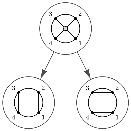
Figure 4: The orthogonal momentum amplituhedron $\mathcal{O}_{2}$ and its boundary poset.

A less trivial example is the three-dimensional $\mathcal{O}_{3}$ (which is equal to $OG_{+}(3)$); its shape and boundary poset are depicted in Figure 5.

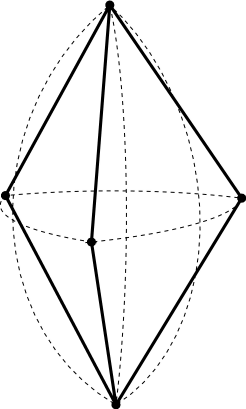
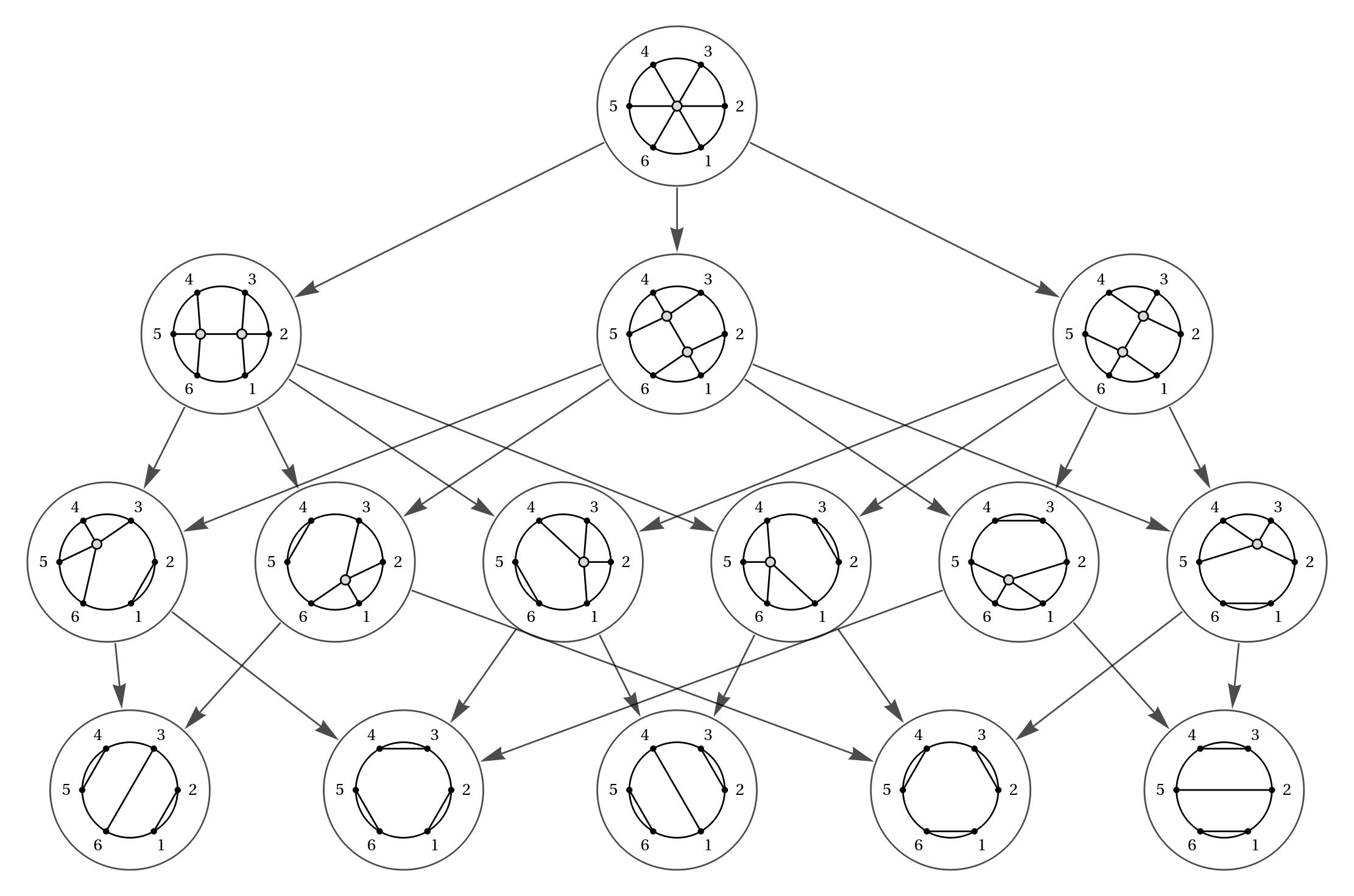
Figure 5: The orthogonal momentum amplituhedron $\mathcal{O}_{3}$ and its boundary poset.

A glimpse into the structure of the $k=4$ orthogonal momentum amplituhedron is given in Table 1, where we have listed all (up to cyclic relabelling) OG forests which appear in the boundary stratification of $\mathcal{O}_{4}$. The complete boundary poset for $\mathcal{O}_{k}$ for $k=4,5,6,7$ can be generated using the orthitroids package, see appendix A.

$\mathrm{dim}_{\mathcal{O}}$	$\mathcal{O}_{4}$	number of boundaries
0		4+8+2=14
1		8+4+8+8=28
2		4+8+8+8=28
3		4+8+8=20
4		8
5		1

Table 1: All types of OG forests that apear in the boundary stratification of $\mathcal{O}_{4}$. We find the Euler characteristic of $\mathcal{O}_{4}$: $\chi=14-28+28-20+8-1=1$.

Before concluding this section, we provide an alternative way of calculating the dimension of boundaries of $\mathcal{O}_{k}$, i.e. the dimension of orthogonal momentum amplituhedron strata labelled by OG forests. Given an OG forest $\Gamma$ of type $\underline{k}$, we define $\dim_{\mathcal{O}}(\Gamma)$ by

$$\dim_{\mathcal{O}}(\Gamma)=\sum_{T\in\text{Trees}(\Gamma)}\dim_{\mathcal{O}}(T)\,,$$ (10)

where for each $T\in\text{Trees}(\Gamma)$

$$\dim_{\mathcal{O}}(T)=\left\{\begin{array}[]{cll}0&,&\text{if }|\mathcal{V}_{\text{ext}}(T)|=2\,,\\ \sum\limits_{v\in\mathcal{V}_{\text{int}}(T)}(\deg(v)-3)&,&\text{if }|\mathcal{V}_{\text{ext}}(T)|>2\,.\end{array}\right.$$ (13)

Here $\deg(v)$ denotes the degree of the internal vertex $v$. We have checked that for every OG forest $\Gamma$ in $\mathcal{O}_{k}$ for $k\leq 7$ we have $\dim(\widetilde{\Phi}_{\Gamma}^{\circ})=\dim_{\mathcal{O}}(\Gamma)$, and we believe the equality holds true for all OG forests.

Finally, we conjecture that the orthogonal momentum amplituhedron $\mathcal{O}_{k}$ is a CW complex with CW decomposition given by $\mathcal{O}_{k}=\sqcup_{\Gamma\in\mathcal{F}_{k}}\Phi^{\circ}_{\Gamma}$ where $\mathcal{F}_{k}$ denote the set of OG forests of type $\underline{k}$.

4 Generating Function and Euler Characteristic

In the previous section we learned that the boundaries of the orthogonal momentum amplituhedron are labelled by OG forests. It is therefore a natural next step to enumerate all OG forests to find the $f$-vector and the Euler characteristic $\chi$ of $\mathcal{O}_{k}$ for all $k$. We will enumerate all OG trees and forests according to their type and orthogonal momentum amplituhedron dimension following the recipe presented in Moerman:2021cjg where (contracted) Grassmannian trees and forests were enumerated according to their type and momentum amplituhedron dimension. In particular, for OG trees one uses the series-reduced planar tree analogue of the Exponential Formula presented in Moerman:2021cjg . To this end, define the statistic $f:2\mathbb{Z}_{\geq 2}\to\mathbb{Q}(q)$ which takes the degree $d\in 2\mathbb{Z}_{\geq 2}$ of an internal vertex and maps it to $f(d)=q^{d-3}$, and let

$$F(x,q):=\sum_{d\in 2\mathbb{Z}_{\geq 2}}f(d)x^{d}=q^{-3}\sum_{k=2}^{\infty}(xq)^{2k}=\frac{x^{4}q}{1-(xq)^{2}}\,,$$ (14)

be the generating function for $f$, i.e. the coefficient of $x^{d}$ in $F(x,q)$, denoted by $[x^{d}]F(x)$, is $f(d)$. Then using the results of Moerman:2021cjg , the number of OG trees of type $\underline{k}$ and with orthogonal momentum amplituhedron dimension $r$ is given by $[x^{2k}q^{r}]\mathcal{G}_{\text{tree}}^{(\mathcal{O})}(x,q)$ where

$$\mathcal{G}_{\text{tree}}^{(\mathcal{O})}(x,q):=x\left(x-\frac{1}{x}F(x,q)\right)^{\langle-1\rangle}_{x}\,,$$ (15)

and $(\ldots)^{\langle-1\rangle}_{x}$ denotes the compositional inverse of $(\ldots)$ with respect to the variable $x$. One can explicitly compute the compositional inverse in (15) using the well-known Lagrange inversion formula to find

$$\mathcal{G}_{\text{tree}}^{(\mathcal{O})}(x,q)=x^{2}\left(1+\sum_{k=1}^{\infty}\sum_{\ell=1}^{\infty}\frac{1}{k}\binom{k}{\ell}\binom{2k+\ell}{2k+1}x^{2k}q^{2k-\ell}\right)\,.$$ (16)

Then one can compute the generating function $\mathcal{G}_{\text{forest}}^{(\mathcal{O})}(x,q)$ which enumerates all OG forests according to their type and orthogonal momentum amplituhedron dimension using Speicher’s analogue of the Exponential Formula for non-crossing partitions Speicher . In particular,

$$\mathcal{G}_{\text{forest}}^{(\mathcal{O})}(x,q):=\frac{1}{x}\left(\frac{x}{1+\mathcal{G}_{\text{tree}}^{(\mathcal{O})}(x,q)}\right)^{\langle-1\rangle}_{x}\,,$$ (17)

or

$$[x^{n}]\mathcal{G}_{\text{forest}}^{(\mathcal{O})}(x,q):=\frac{1}{n+1}[x^{n}]\left(1+\mathcal{G}_{\text{tree}}^{(\mathcal{O})}(x,q)\right)^{n+1}\,.$$ (18)

Using this formula, one can find the $f$-vector for the orthogonal momentum amplituhedron $\mathcal{O}_{k}$. The results for the first few values of $k$ are displayed in Table 2.

$k$	$f$-vector	$\chi$
2	$(1,2)$	1
3	$(1,3,6,5)$	1
4	$(1,8,20,28,28,14)$	1
5	$(1,15,65,145,195,180,120,42)$	1
6	$(1,24,168,562,1131,1518,1430,990,495,132)$	1
7	$(1,35,364,1764,5019,9436,12558,12285,9009,5005,2002,429)$	1

Table 2: The $f$-vector and Euler characteristic $\chi$ of $\mathcal{O}_{k}$ for $k\leq 7$.

One can also easily compute the Euler characteristic of $\mathcal{O}_{k}$ using this formula. Recall that for a CW complex, its Euler characteristic is defined by the alternating sum $\chi=n_{0}-n_{1}+n_{2}-n_{3}+\ldots$ where $n_{r}$ denotes the number of boundaries with dimension $r$. Consequently, the Euler characteristic for $\mathcal{O}_{k}$ can be computed as $[x^{2k}]\mathcal{G}_{\text{forest}}^{(\mathcal{O})}(x,-1)$. To this end, first evaluate $\mathcal{G}_{\text{tree}}^{(\mathcal{O})}(x,q)$ at $q=-1$:

$$\mathcal{G}_{\text{tree}}^{(\mathcal{O})}(x,-1)=x\left(\frac{x}{1-x^{2}}\right)^{\langle-1\rangle}_{x}=-\frac{1}{2}(1+\sqrt{1+4x^{2}})\,.$$ (19)

Then

$$\frac{x}{1+\mathcal{G}_{\text{tree}}^{(\mathcal{O})}(x,-1)}=\frac{2x}{1-\sqrt{4x^{2}+1}}=-\frac{1}{2x}(1+\sqrt{1+4x^{2}})=\left(\frac{x}{1-x^{2}}\right)^{\langle-1\rangle}_{x}\,,$$ (20)

and

$$\mathcal{G}_{\text{forest}}^{(\mathcal{O})}(x,-1)=\frac{1}{x}\left(\frac{x}{1+\mathcal{G}_{\text{tree}}^{(\mathcal{O})}(x,q)}\right)^{\langle-1\rangle}_{x}=\frac{1}{x}\frac{x}{1-x^{2}}=\frac{1}{1-x^{2}}=\sum_{k=0}^{\infty}x^{2k}\,.$$ (21)

Consequently, the Euler characteristic of $\mathcal{O}_{k}$ is $[x^{2k}]\mathcal{G}_{\text{forest}}^{(\mathcal{O})}(x,-1)=1$.

5 Diagrammatic Map between Boundaries of $\overline{\mathcal{M}}_{0,2k}^{+}$ and $\mathcal{O}_{k}$

In this section we highlight an interesting relation between the associahedron $A_{2k-3}$ and the orthogonal momentum amplituhedron $\mathcal{O}_{k}$. First notice that both geometries are $(2k-3)$-dimensional. Moreover, it was proposed in He:2021llb that one can map the positive moduli space $\mathcal{M}^{+}_{0,2k}\coloneqq\{\sigma_{1}<\sigma_{2}<\cdots<\sigma_{2k}\}/\mathrm{SL}(2,\mathbb{R})$ directly to $\mathcal{O}_{k}$ using the ‘twistor-string map’

$$\Phi_{\Lambda}\colon\mathcal{M}^{+}_{0,2k} \to G(k,k+2)$$ (22)

$$\sigma \mapsto Y_{\alpha}^{A}=C_{\alpha i}(\sigma)\Lambda_{i}^{A}\,.$$

Here $\sigma=\{\sigma_{1},\sigma_{2},\cdots,\sigma_{2k}\}\in\mathcal{M}^{+}_{0,2k}$ is intermediately mapped to an element $C_{\alpha i}(\sigma)$ of $OG_{+}(k)$ through the Veronese map

$$\begin{pmatrix}1&1&\cdots&1\\ \sigma_{1}&\sigma_{2}&\cdots&\sigma_{2k}\end{pmatrix}\mapsto C_{\alpha i}(\sigma)=\begin{pmatrix}t_{1}&t_{2}&\cdots&t_{2k-1}&1\\ t_{1}\sigma_{1}&t_{2}\sigma_{2}&\cdots&t_{2k-1}\sigma_{2k-1}&\sigma_{2k}\\ \vdots&\vdots&\ddots&\vdots&\vdots\\ t_{1}\sigma_{1}^{k-1}&t_{2}\sigma_{2}^{k-1}&\cdots&t_{2k-1}\sigma_{2k-1}^{k-1}&\sigma_{2k}^{k-1}\end{pmatrix},$$ (23)

with $t_{i}^{2}=(-1)^{i}\frac{\prod_{j\neq 2k}(\sigma_{2k}-\sigma_{j})}{\prod_{j\neq i}(\sigma_{i}-\sigma_{j})}$. The map (22) is conjectured to provide a diffeomorphism between the interior of $\mathcal{M}^{+}_{0,2k}$ and the interior of $\mathcal{O}_{k}$. On the other hand, it is well known that the Deligne-Mumford compactification $\overline{\mathcal{M}}_{0,2k}^{+}$ of the positive moduli space $\mathcal{M}^{+}_{0,2k}$ has the boundary structure of an associahedron Deligne1969 . It is further conjectured that $\overline{\mathcal{M}}^{+}_{0,2k}$ is diffeomorphic to the ABHY associahedron $A_{2k-3}$ through the scattering equations Arkani-Hamed:2017mur . Since the boundary structure of the orthogonal momentum amplituhedron differs from the one of an associahedron, it implies that the map (22) does not extend to a diffeomorphism between the compactification $\overline{\mathcal{M}}_{0,2k}^{+}$ and the closure of $\mathcal{O}_{k}$. Even more well-known is the fact that the boundaries of the ABHY associahedron can be labelled by planar tree Feynman diagrams. In this section we propose a diagrammatic, partial-order-preserving map from the boundaries of the associahedron $A_{2k-3}$ to boundaries of $\mathcal{O}_{k}$ and conjecture that this extends the map (22) to a homeomorphism between $\overline{\mathcal{M}}_{0,2k}^{+}$ and $\mathcal{O}_{k}$.

Note that the Feynman diagrams appearing in the boundary stratification of $A_{2k-3}$ can be labelled by the planar Mandelstam invariants that correspond to the internal edges of the diagram. We now propose the following map from planar tree Feynman diagrams to OG forests: given a planar tree Feynman diagram, remove all internal edges which correspond to even-particle planar Mandelstam invariants and replace all vertices of degree $2$ with a single edge. It is not difficult to convince oneself that the resulting diagram is an OG forest. Furthermore, it is clear that every OG forest can be obtained from at least one planar tree Feynman diagram, as can be seen by starting from an OG forest and connecting all disconnected parts by internal edges. Since all planar tree Feynman diagrams on $2k$ leaves appear in the boundary stratification of $A_{2k-3}$, and given our knowledge of the boundary stratification of $\mathcal{O}_{k}$ discussed in Section 3, it is clear that the map defined above is surjective from boundary elements of $A_{2k-3}$ to boundary elements of $\mathcal{O}_{k}$. We furthermore claim that the poset induced by the boundary stratification of $A_{2k-3}$ will result in the poset corresponding to the boundary stratification of $\mathcal{O}_{k}$. The simplest example is the case when $k=2$, where both the associahedron $A_{1}$ and the orthogonal momentum amplituhedron $\mathcal{O}_{2}$ are segments. The first non-trivial example is the one for $k=3$ where the $f$-vector for the associahedron $A_{3}$ given by $(1,9,21,14)$ reduces to the $f$-vector of $\mathcal{O}_{3}$ given by $(1,3,6,5)$. This is depicted in Figure 6 at the level of geometry and in Figure 7 at the level of boundary posets.

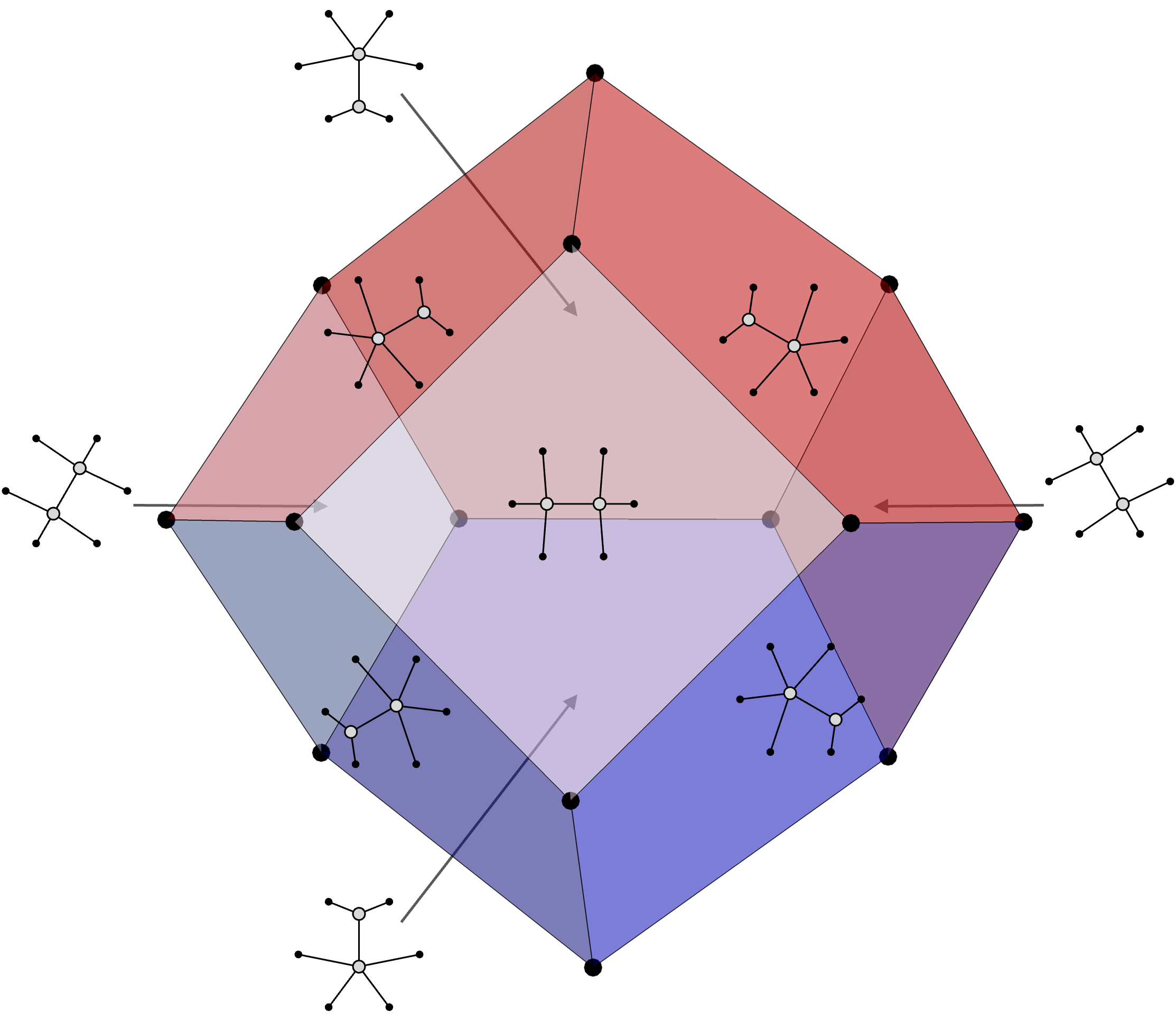
   $$\to$$

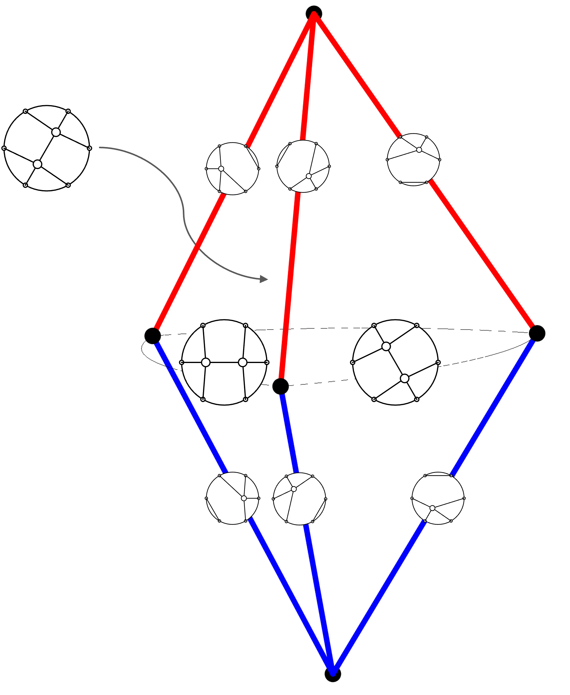
Figure 6: Reduction of the three-dimensional associahedron to the orthogonal momentum amplituhedron $\mathcal{O}_{3}$.

We have performed direct calculations for $k\leq 5$ and explicitly confirmed that the boundary stratification of the associahedron reduces to the boundary stratification found in Section 3, and we believe this continues to be be true for all $k$.

The reduction discussed above also allows us to explain some of the statements about physical boundaries of $\mathcal{O}_{k}$ made in Huang:2021jlh ; He:2021llb . In particular, let us take a closer look at the codimension-one boundaries of the associahedron. Recall that the interior of the associahedron $A_{2k-3}$ can be represented by a Feynman diagram with a single degree $2k$ vertex. Going to one of its codimension-one boundaries corresponds to dissolving the degree $2k$ vertex into two vertices of degree $(2k-p+1)$ and $(p+1)$, with $2\leq p\leq 2k-2$, connected via a single edge. For odd (resp., even) $p$, the internal edge corresponds to an odd-particle (resp., even-particle) Mandelstam variable. Via the map defined above, Feynman diagrams with a single edge corresponding to an odd-particle Mandelstam variable will remain unchanged, and we thus interpret the Feynman diagram as an OG tree without changing anything. From (13), the resulting OG tree will have an orthogonal momentum amplituhedron dimension of $(2k-p+1-3)+(p+1-3)=2k-4$, and therefore labels a codimension-one boundary of $\mathcal{O}_{k}$. On the other hand, Feynman diagrams with a single edge corresponding to an even-particle Mandelstam variable will be mapped to OG forests consisting of two disconnected OG trees, each consisting of a single vertex of degree $2k-p$ and degree $p$, respectively. From (10) we find that these OG trees have orthogonal momentum amplituhedron dimension $(2k-p-3)+(p-3)=2k-6$, with an exception for the cases where $p=2$ or $p=2k-2$ when the dimension of the OG forest is $2k-5$. These results agree with the discussions about the physical boundaries of $\mathcal{O}_{k}$ found in He:2021llb ; Huang:2021jlh .

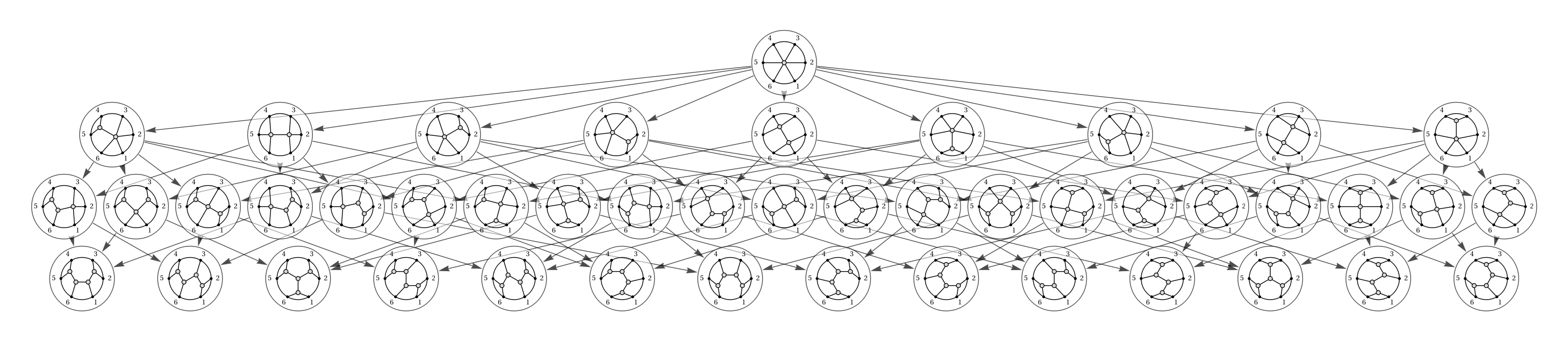
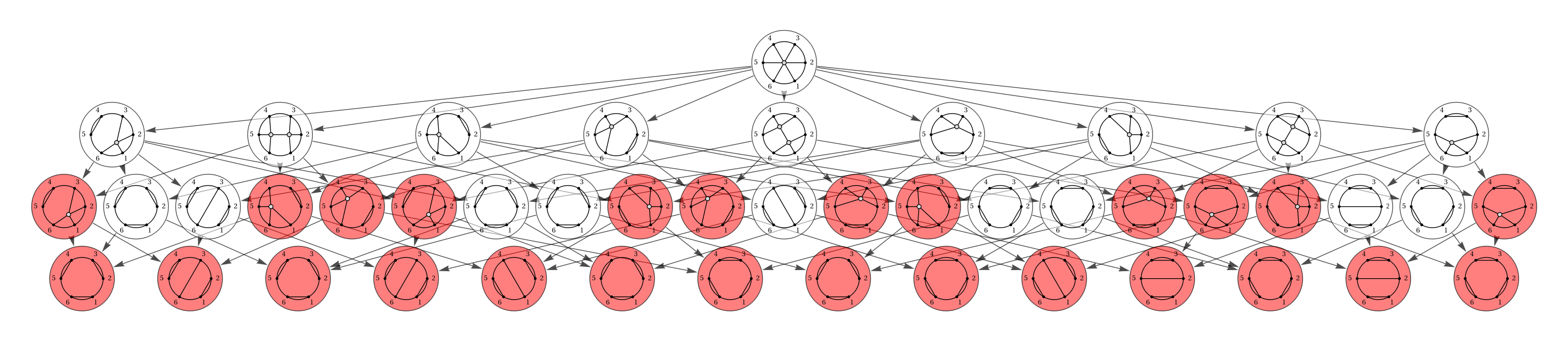
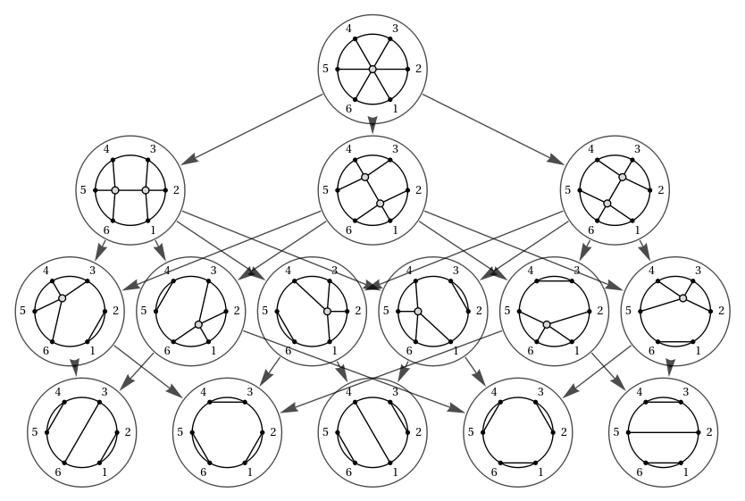
Figure 7: The top and middle Hasse diagrams depict the poset of boundaries of $A_{3}$ with nodes labelled by planar trees on $6$ leaves (top) and OG forests of type $3$ (middle). In the middle Hasse diagram, nodes with parents labelled by the same OG forest are coloured red. The bottom Hasse diagram is obtained from the middle one by identifying nodes labelled by the same OG forest.

Appendix A Mathematica package orthitroid

While working on this project we have developed a Mathematica package orthitroids which contains many useful functions for studying the positive orthogonal Grassmannian and the orthogonal momentum amplituhedron. It parallels some of the functionality of the positroids package Bourjaily:2012gy and the amplituhedronBoundaries package Lukowski:2020bya . In this appendix we provide a list of some useful functions from the orthitroids package. We use the following three name spaces for distinguishing functions:

• opos – for functions related to the othogonal positive Grassmannian $OG_{+}(k)$;

• omom – for functions related to the orthogonal momentum amplituhedron $\mathcal{O}_{k}$;

• mod – for functions related to the Deligne-Mumford compactification of the positive part of the moduli space of $2k$ points on the Riemann sphere $\overline{\mathcal{M}}_{0,2k}^{+}$.

A.1 Positive Orthogonal Grassmannian

• oposTopCell[ k  ]​ : returns the permutation for the top-dimensional orthitroid cell of the positive orthogonal Grassmannian.

• oposPermToCrossing[ perm  ]​ : returns a crossing diagram for the permutation perm.

  • oposPermToCrossing[{{1,3},{2,7},{4,6},{5,8}}]

  • 

• oposPermToYoungNice[ perm  ]​ : returns the Young diagram for the orthitroid cell labelled by the permutation perm.

  • oposPermToYoungNice[{{1,3},{2,7},{4,6},{5,8}}]

  • 

• oposPermToYoungReducedNice[ perm  ]​ : returns the reduced (folded) Young diagram for the orthitroid cell labelled by the permutation perm.

  • oposPermToYoungReducedNice[{{1,3},{2,7},{4,6},{5,8}}]

  • 

• oposDimension[ perm  ]​ : returns the positive orthogonal Grassmannian dimension of the orthitroid cell labelled by the permutation perm.

  • oposDimension[{{1,3},{2,7},{4,6},{5,8}}]

  • 3

• oposBoundary[ perm  ]​ : returns the list of codimension-one boundaries of the orthitroid cell labelled by the permutation perm.

  • oposBoundary[{{1,3},{2,7},{4,6},{5,8}}]

  • {{{1,2},{3,7},{4,6},{5,8}},{{1,3},{2,5},{4,6},{7,8}},{{1,3},{2,7},{4,5},{6,8}},{{1,7},{2,3},{4,6},{5,8}},{{1,3},{2,8},{4,6},{5,7}},{{1,3},{2,7},{4,8},{5,6}}}

• oposInverseBoundary[ perm  ]​ : returns the list of orthitroid cells which have the orthitroid cell labelled by the permutation perm as a codimension-one boundary.

  • oposInverseBoundary[{{1,3},{2,7},{4,6},{5,8}}]

  • {{{1,4},{2,7},{3,6},{5,8}},{{1,5},{2,7},{3,8},{4,6}},{{1,3},{2,6},{4,7},{5,8}}}

• oposStratification[ perm  ]​ : returns all boundaries (of all codimensions) of the orthitroid cell labelled by the permutation perm.

• oposInverseStratification[ perm  ]​ : returns the list of orthitroid cells which have the orthitroid cell labelled by the permutation perm in its boundary stratification.

• oposPermToMat[ perm  ]​ : returns a matrix parametrizing the orthitroid cell labelled by the permutation perm with $c_{i}=\cosh(\theta_{i})$ and $s_{i}=\sinh(\theta_{i})$.

  • MatrixForm@oposPermToMat[{{1,3},{2,7},{4,6},{5,8}}]

  • $\left(\begin{array}[]{cccccccc}1&0&-s_{3}&0&0&0&-c_{3}s_{1}&-c_{1}c_{3}\\ 0&1&c_{3}&0&0&0&s_{1}s_{3}&c_{1}s_{3}\\ 0&0&0&1&0&-s_{2}&-c_{1}c_{2}&-c_{2}s_{1}\\ 0&0&0&0&1&c_{2}&c_{1}s_{2}&s_{1}s_{2}\\ \end{array}\right)$

A.2 Orthogonal Momentum Amplituhedron

• omomPermToForest[ perm  ]​ : returns the OG forest for the permutation perm.

  • omomPermToForest[{{1,3},{2,7},{4,6},{5,8}}]

  • 

• omomDimension[ perm  ]​ : returns the orthogonal momentum amplituhedron dimension of the cell labelled by the permutation perm.

  • omomDimension[{{1,3},{2,7},{4,6},{5,8}}]

  • 3

• omomBoundary[ perm  ]​ : returns the list of codimension-one boundaries of the orthogonal momentum amplituhedron cell labelled by the permutation perm.

• omomInverseBoundary[ perm  ]​ : returns the list of orthogonal momentum amplituhedron cells which have the cell labelled by the permutation perm as a codimension-one boundary.

  • omomInverseBoundary[{{1,3},{2,7},{4,6},{5,8}}]

  • {{{1,3},{2,6},{4,7},{5,8}},{{1,5},{2,7},{3,8},{4,6}}}

• omomStratification[ perm  ]​ : returns all boundaries (of all codimensions) of the orthogonal momentum amplituhedron cell labelled by the permutation perm.

• omomInverseStratification[ perm  ]​ : returns the list of orthogonal momentum amplituhedron cells which have the cell labelled by the permutation perm in its boundary stratification.

A.3 Moduli Space

• modDiagonalsToPlanarTree[ k  ]​[ listOfDiags  ]​ : returns a planar tree on $2\text{\tt{\color[rgb]{0.1,0.55,0.25}{\sl k}}}$ leaves which is dual to the dissection of a regular $2\text{\tt{\color[rgb]{0.1,0.55,0.25}{\sl k}}}$-gon specified by the diagonals in listOfDiags.

  • modDiagonalsToPlanarTree[4][{{1,3},{1,5}}]

  • 

• modDiagonalsToForest[ k  ]​[ listOfDiags  ]​ : returns the corresponding OG forest of type $\underline{\text{\tt{\color[rgb]{0.1,0.55,0.25}{\sl k}}}}$ obtained from modDiagonalsToPlanarTree[ k ]​[ listOfDiags ]​  via the map described in this paper.

  • modDiagonalsToForest[4][{{1,3},{1,5}}]

  •

References

- (1) N. Arkani-Hamed, Y. Bai and T. Lam, “Positive Geometries and Canonical Forms”, JHEP 1711, 039 (2017), arxiv:1703.04541.
- (2) N. Arkani-Hamed and J. Trnka, “The Amplituhedron”, JHEP 1410, 030 (2014), arxiv:1312.2007.
- (3) D. Damgaard, L. Ferro, T. Lukowski and M. Parisi, “The Momentum Amplituhedron”, JHEP 1908, 042 (2019), arxiv:1905.04216.
- (4) Y.-t. Huang, R. Kojima, C. Wen and S.-Q. Zhang, “The orthogonal momentum amplituhedron and ABJM amplitudes”, arxiv:2111.03037.
- (5) S. He, C.-K. Kuo and Y.-Q. Zhang, “The momentum amplituhedron of SYM and ABJM from twistor-string maps”, arxiv:2111.02576.
- (6) N. Arkani-Hamed, Y. Bai, S. He and G. Yan, “Scattering Forms and the Positive Geometry of Kinematics, Color and the Worldsheet”, JHEP 1805, 096 (2018), arxiv:1711.09102.
- (7) T. Łukowski, “On the Boundaries of the m=2 Amplituhedron”, arxiv:1908.00386.
- (8) T. Łukowski and R. Moerman, “Boundaries of the amplituhedron with amplituhedronBoundaries”, Comput. Phys. Commun. 259, 107653 (2021), arxiv:2002.07146.
- (9) R. Moerman and L. K. Williams, “Grass trees and forests: Enumeration of Grassmannian trees and forests, with applications to the momentum amplituhedron”, arxiv:2112.02061.
- (10) A. Postnikov, “Positive Grassmannian and polyhedral subdivisions”, arxiv:1806.05307.
- (11) A. Postnikov, “Total positivity, Grassmannians, and networks”, math/0609764.
- (12) J. L. Bourjaily, “Positroids, Plabic Graphs, and Scattering Amplitudes in Mathematica”, arxiv:1212.6974.
- (13) Y.-T. Huang and C. Wen, “ABJM amplitudes and the positive orthogonal grassmannian”, JHEP 1402, 104 (2014), arxiv:1309.3252.
- (14) J. Kim and S. Lee, “Positroid Stratification of Orthogonal Grassmannian and ABJM Amplitudes”, JHEP 1409, 085 (2014), arxiv:1402.1119.
- (15) L. Ferro, T. Łukowski and R. Moerman, “From momentum amplituhedron boundaries to amplitude singularities and back”, JHEP 2007, 201 (2020), arxiv:2003.13704.
- (16) R. Speicher, “Multiplicative functions on the lattice of noncrossing partitions and free convolution”, Math. Ann. 298, 611 (1994), https://doi.org/10.1007/BF01459754.
- (17) P. Deligne and D. Mumford, “The irreducibility of the space of curves of given genus”, Publications Mathématiques de l’Institut des Hautes Études Scien 36, 75 (1969), https://doi.org/10.1007/BF02684599.