Action complexity in the presence of defects
and boundaries

Roberto Auzzi^a,b, Stefano Baiguera^c,

Sara Bonansea^d and Giuseppe Nardelli^a,e

^a Dipartimento di Matematica e Fisica, Università Cattolica del Sacro Cuore,
Via della Garzetta 48, 25133 Brescia, Italy

^b INFN Sezione di Perugia, Via A. Pascoli, 06123 Perugia, Italy

^c Department of Physics, Ben-Gurion University of the Negev,
Beer Sheva 84105, Israel

^d The Niels Bohr Institute, University of Copenhagen,
Blegdamsvej 17, DK-2100 Copenhagen Ø, Denmark

^e TIFPA - INFN, c/o Dipartimento di Fisica, Università di Trento,
38123 Povo (TN), Italy

E-mails: roberto.auzzi@unicatt.it, baiguera@post.bgu.ac.il,

sarabonansea@gmail.com, giuseppe.nardelli@unicatt.it

• The holographic complexity of formation for the AdS₃ $2$-sided Randall-Sundrum model and the AdS₃/BCFT₂ models is logarithmically divergent according to the volume conjecture, while it is finite using the action proposal. One might be tempted to conclude that the UV divergences of the volume and action conjectures are always different for defects and boundaries in two-dimensional conformal field theories. We show that this is not the case. In fact, in Janus AdS₃ we find that both volume and action proposals provide the same kind of logarithmic divergences.

1 Introduction

Starting from the seminal work by Ryu and Takayanagi [1] on the holographic dual of Entanglement Entropy (EE), the development of the AdS/CFT correspondence [2] intertwined with quantum information. One of the characters that recently entered the scene is computational complexity, which may provide a field theory dual to the asymptotic growth of the Einstein-Rosen Bridge (ERB) after long time scales [3, 4]. Heuristically, quantum computational complexity estimates the difficulty to build a target state starting from a simple, usually unentangled, reference state. This is done by counting the number of steps needed to reach the target state from the reference one, picking unitaries from a universal set of elementary operations [5, 6]. This problem is of primary importance in the context of quantum infomation [7]. Two main conjectures have been proposed as holographic duals of computational complexity:

• Complexity=volume (CV) [8], in which complexity is proportional to the volume of the maximal slices anchored to the boundary

  $$\mathcal{C}_{V}\sim\frac{\mathcal{V}}{GL}\,,$$ (1.1)

  where $\mathcal{V}$ is the maximal volume of the ERB, $G$ the Newton’s constant and $L$ the AdS radius.

• Complexity=action (CA) [9, 10], in which complexity is proportional to the gravitational action evaluated on the Wheeler DeWitt (WDW) patch, which is the bulk domain of dependence of the above-mentioned spatial slice

  $$\mathcal{C}_{A}=\frac{I_{\rm WDW}}{\pi\hbar}\,,$$ (1.2)

  where $I_{\rm WDW}$ is the on-shell gravitational action evaluated on the WDW patch. We will use natural units for the Planck’s constant $\hbar=1.$

In spite that both the CV and the CA proposals have been investigated in several contexts [11, 12, 13, 14, 15, 16, 17, 18, 19, 20, 21, 22, 23, 24, 25], we are still far away from a definitive understanding of complexity conjectures. One of the most important open problems is a satisfactory definition of the computational complexity on the field theory side. Up to now, most of the developments have been done in quantum-mechanical systems with a finite number of degrees of freedom [26, 27, 28, 29, 30] and in free field theories [31, 32, 33, 34], but a precise definition in interacting CFTs is still lacking (see e.g. [35, 36, 37, 38, 39, 40] for some progresses in this direction). See also [41] for the case of Topological Quantum Field Theory. See [42, 43] for reviews.

To achieve further insights, it may be useful to take inspiration from the EE, for which both the holographic and the field theory side of the duality are under control. In field theory, the definition of EE requires a splitting of the system in two complementary subregions. In the gravity theory, the entropy is computed as the area delimited by the Ryu-Tayanagi (RT) surface [1], which is attached on the boundary of the given subsystem. It is then natural to conjecture that subsystems play an important role also for complexity. Indeed, several definitions have been proposed to generalise the concept of computational complexity to mixed states and subregions [44, 45]. On the holographic side, both the volume and action conjectures have natural extensions to the case of subsystems. The CV generalisation [46] requires to compute the maximal volume of the codimension-one bulk surface $\mathcal{R}_{A}$ anchored to a subregion $A$ on the boundary and delimited by its Ryu-Tayanagi (RT) surface

$$\mathcal{C}_{V}(A)\sim\frac{\mathcal{V}(\mathcal{R}_{A})}{GL}\,.$$ (1.3)

The CA subregion proposal [12] requires instead to calculate the gravitational action in the intersection between the WDW patch and the Entanglement Wedge (EW), which is the bulk domain of dependence of the RT surface:

$$\mathcal{C}_{A}(A)=\frac{I_{\rm WDW\cap EW}}{\pi\hbar}\,.$$ (1.4)

Subregion complexity has then been investigated for several configurations [47, 48, 49, 50, 51, 52, 53, 54], including the Banados-Teitelboim-Zanelli (BTZ) [55] black hole.

At the qualitative level, the volume and the action conjectures share many important features, such as the linear growth at late time [8, 9, 10], the structure of divergences [16, 12] and the switch-back effect [56]. A certain degree of arbitrariness is expected in defining computational complexity, due to the choice of the reference state and of the allowed computational gates. Consequently, CV and CA (and their further generalizations [14, 25]) might correspond to different ways to define complexity on the field theory side. It is then crucial to focus on the examples where CV and CA provide different results. Systems with defects may provide such examples [57]. Indeed, this is precisely what happens for the $2$-sided Randall-Sundrum ($2$-RS) model [58] in AdS₃. In this case, the contribution to the CV due to the defect contains a logarithmic divergence in the UV regulator, while CA is not influenced by the presence of the defect [59]. This is true both for the complexity of the total space and for the subregion complexity of an interval centered around the defect, once the subtraction of the vacuum result is performed (complexity of formation).

Boundaries are related to defects via the folding trick [60], and so we expect a similar behaviour for their contribution to complexity. One can consider also the $1$-sided version of the Randall-Sundrum model, which is dual to a Boundary Conformal Field Theory (BCFT). In the following we shall refer to this case as the AdS_d+1/BCFT_d model [61, 62, 63]. Complexity in AdS_d+1/BCFT_d model was investigated in [64, 65]. For $d=2$, the contribution of the defect to CV is again logarithmically divergent, while the contribution to CA is finite. For $d>2$, instead, both volume and action give rise to the same type of divergences. These results were established in [64, 65] for the case of total complexity. The behaviour of the UV divergences should be the same also for the complexity of a subregion which contain the defect, because (by locality) the UV divergences are expected to come from the region nearby the defect. This was explicitly checked in AdS₃/BCFT₂ for CV in [64]. In section 4 we will check this claim also for CA.

Studying these examples, one is tempted to conclude that, for defects and boundaries in 2-dimensional field theories, the UV divergences of CV and CA are different. It is important to understand if this is a general feature of every two-dimensional theory with defects. In this paper, we show that this is not the case.

To this purpose, we study complexity in Janus AdS₃. This geometry is a dilatonic deformation [66, 67] of pure AdS₃, which can be embedded in type IIB supergravity. Due to technical reasons related to the regularization of IR-divergences, in this background it is natural to directly work with the case of subregions. In fact, the length of the subregion provides a natural IR regulator. In [68] we considered the volume conjecture for Janus AdS₃ and we found that, also in this case, the contribution to complexity due to the defect is logarithmically divergent. We performed the calculation with three different regularizations (Fefferman-Graham, single and double cutoff regularizations [69, 70, 71]) and we checked that the coefficient of the logarithmically divergent term is independent of the regularization choice.

In section 3 we will study the subregion action complexity for Janus AdS₃ and we will find that, contrarily to what happens in the three dimensional $2$-RS and AdS/BCFT models, the contribution to complexity due the defect is logarithmically divergent, as it happens for the volume complexity. We summarise the results for the contribution of the defect to CV and CA in various models in table 1.

	$\Delta\mathcal{C}_{V}(l)$	$\Delta\mathcal{C}_{A}(l)$
$2$-sided Randall-Sundrum	$\frac{2}{3}c\,\eta_{\rm RS}\,\log\left(\frac{l}{\,\delta}\right)+\text{finite}$	$0$
AdS3/BCFT2	$\frac{2}{3}c\,\eta_{\rm BCFT}\,\log\left(\frac{l}{\,\delta}\right)+\text{finite}$	$\mathrm{finite}$
Janus AdS3	$\frac{2}{3}c\,\eta_{\rm JAdS}\,\log\left(\frac{l}{\,\delta}\right)+\text{finite}$	$\frac{2c}{3\pi^{2}}P(\gamma,\tilde{L}/L)\log\left(\frac{l}{\delta}\right)+\mathrm{finite}$

Table 1: Behaviour of the contributions of the defect $\Delta\mathcal{C}_{V}$ and $\Delta\mathcal{C}_{A}$ to the subregion complexity, for an interval of length $l$ for CV and CA, respectively. The coefficients of the log divergences $\eta$ are specific of the details of the defect or boundary. In the case of Janus geometry, $\eta_{\rm JAdS}$ is given in eq. (3.110). For the other models, the $\eta$ coefficients can be extracted from [59, 64, 65, 68]; their specific values are not essential for the present discussion. The function $P(\gamma,\tilde{L}/L)$ is given in eq. (3.108).

The first comment comes from reading the table by columns. While in the volume case the three models have a common logarithmic divergence, for the action there are three different behaviours:

• The action of the $2$-RS model is completely blind to the presence of the defect, because it does not depend on the brane tension. Therefore, after subtracting the vacuum part of the action, we find an identically zero $\Delta\mathcal{C}_{A}$.

• The action of the AdS/BCFT model is modified by the presence of the end-of-the-world brane because the action depends on the tension of the brane. After subtracting the vacuum contribution, the divergences cancel and $\Delta\mathcal{C}_{A}$ is finite.

• In the Janus geometry, the divergent part of the action is modified by the presence of the defect. After subtracting the vacuum part, the log divergence survives in $\Delta\mathcal{C}_{A}$ and depends on the parameter $\gamma$ of the Janus solution.

Another perspective that can be taken is to compare the volume and the action results for each background, i.e. we read Table 1 by rows. In this case we note that:

• The $2$-RS model distinguishes between volume and action: the former has a logarithmic divergence dependent on the tension of the defect, while the latter is identically zero.

• The AdS/BCFT model distinguishes between volume and action, but in a milder way. Only the finite term in the action depends on the brane tension. Furthermore, in higher dimensions ($d>2$) the same divergences reappear both in the action and in the volume [65].

• For the Janus AdS₃ geometry both the volume and the action have a logarithmic divergence dependent on the deformation parameter $\gamma$.

The manuscript is organized as follows. In section 2 we introduce the Janus AdS₃ and the AdS₃/BCFT₂ geometries, we list all the terms entering the gravitational action and we discuss the regularization prescriptions to systematically treat UV divergences. In sections 3 and 4 we derive the results collected in Table 1 by performing the calculation of subregion action complexity for the Janus and the BCFT backgrounds, respectively. Further open problems are discussed in section 5. The appendices contain technical details.

2 Preliminaries

In this section we introduce the main characters entering the computation of subsystem complexity. In section 2.1 we will review the Janus AdS₃ geometry, dual to an interface CFT (ICFT) where the coupling constant is different on each side of the interface. In section 2.2 we will describe the AdS/BCFT model. In the remaining sections, we will discuss the gravitational action in the presence of null boundaries and the regularizations adopted in our calculation.

2.1 Janus AdS₃ geometry

The Janus AdS₃ geometry is a solution of type IIB supergravity which preserves the isometry subgroup $\mathrm{SO}(1,2)\times\mathrm{SO}(4)$ of the background geometry $\mathrm{AdS}_{3}\times S^{3}\times M_{4},$ where $M_{4}$ is a four-dimensional compact manifold [67]. Upon dimensional reduction we obtain Einstein gravity coupled to a dilaton field $\phi$, i.e.

$$I=\frac{1}{16\pi G}\int d^{3}x\sqrt{-g}\,\left(R-\partial^{a}\phi\partial_{a}\phi+\frac{2}{L^{2}}\right)\,,$$ (2.1)

where $L$ the AdS₃ radius. The metric of the Janus solution reads

$$ds_{3}^{2}=L^{2}f(\mu)\cos^{2}\mu\,ds^{2}_{\mathrm{AdS}_{3}}\,,\qquad ds^{2}_{\mathrm{AdS}_{3}}=\frac{1}{\cos^{2}\mu}\left(d\mu^{2}+ds^{2}_{\mathrm{AdS}_{2}}\right)\,.$$ (2.2)

Unless otherwise specified, the two-dimensional AdS slices will be parametrized using Poincaré coordinates

$$ds^{2}_{\mathrm{AdS}_{2}}=\frac{1}{z^{2}}\left(dz^{2}-dt^{2}\right)\,.$$ (2.3)

The profile function $f$ and the dilaton $\phi$ are given by [72]

$$f(\mu) = \frac{\alpha_{+}^{2}}{\mathrm{sn}^{2}\left(\alpha_{+}(\mu+\mu_{0})|m\right)}\,,$$

$$\phi(\mu) = \phi_{0}+\sqrt{2}\log\left[\mathrm{dn}\left(\alpha_{+}(\mu+\mu_{0})|m\right)-\sqrt{m}\,\mathrm{cn}\left(\alpha_{+}(\mu+\mu_{0})|m\right)\right]\,,$$ (2.4)

where

$$\alpha_{\pm}^{2}=\frac{1}{2}\left(1\pm\sqrt{1-2\gamma^{2}}\right)\,,\qquad m=\left(\frac{\alpha_{-}}{\alpha_{+}}\right)^{2}\,,\qquad\mu_{0}=\frac{\mathbb{K}(m)}{\alpha_{+}}\,.$$ (2.5)

The conventions on the Jacobi elliptic functions are collected in Appendix A. The parameter $\gamma\in[0,\frac{1}{\sqrt{2}}]$ specify the details of the dilatonic deformation. The range of the angular coordinate is $\mu\in[-\mu_{0},\mu_{0}]$ with $\mu_{0}\geq\pi/2.$ The value $\gamma=0$ corresponds to vacuum AdS space with constant dilaton, $\mu_{0}=\pi/2$ and $f(\mu)=\frac{1}{\cos^{2}\mu}$. The case $\gamma=\frac{1}{\sqrt{2}}$ corresponds to an infinite dilaton excursion between the two sides of the Janus interface.

In some cases, it is convenient to change variables from $\mu$ to $y$ in the following way

$$d\mu=\frac{dy}{\sqrt{f(y)}}\,,\qquad ds^{2}=L^{2}\left(f(y)ds^{2}_{\mathrm{AdS_{2}}}+dy^{2}\right)\,.$$ (2.6)

In this coordinate system, $y\in[-\infty,\infty]$ and these two extrema correspond to the two sides of the boundary where the dual interface field theory lives. In this system the profile functions are

$$f(y) = \frac{1}{2}\left(1+\sqrt{1-2\gamma^{2}}\cosh(2y)\right)\,,$$

$$\phi(y) = \phi_{0}+\frac{1}{\sqrt{2}}\log\left(\frac{1+\sqrt{1-2\gamma^{2}}+\sqrt{2}\gamma\tanh y}{1+\sqrt{1-2\gamma^{2}}-\sqrt{2}\gamma\tanh y}\right)\,.$$ (2.7)

This geometry admits a dual description in terms of a two-dimensional interface CFT where the deformation is produced by a marginal operator $O(x)$ with couplings $J_{\pm}\int d^{2}x\,O(x)$ on each side of the boundary, such that

$$J_{\pm}=\lim_{y\rightarrow\pm\infty}\phi(y)\,.$$ (2.8)

Since the Janus deformation is associated with an exactly marginal operator, it does not change the central charge of the CFT.

2.2 AdS₃/BCFT₂ model

The AdS/BCFT model can be thought as a $1$-sided version of the Randall-Sundrum setup [58], in which the brane intersects the asymptotically AdS boundary. The AdS₃/BCFT₂ model was studied in detail in [61, 62, 63] to describe a QFT which is restricted to live on a half plane of flat space, i.e. along the portion of spacetime given by $x\geq 0$ in the Minkowski metric, as shown in Fig. 1. The bulk dual description corresponds to AdS₃ space with a boundary given by an end-of-the-world brane $\mathcal{Q}$ of tension $T$. We use the AdS metric in Poincaré coordinates

$$ds^{2}=\frac{L^{2}}{z^{2}}\left(-dt^{2}+dz^{2}+dx^{2}\right)\,,$$ (2.9)

and the gravitational action is supplemented by a codimension-one term

$$I=\frac{1}{16\pi G}\int_{\mathcal{B}}d^{3}x\,\sqrt{-g}\,\left(R+\frac{2}{L^{2}}\right)+\frac{1}{8\pi G}\int_{\mathcal{Q}}d^{2}x\,\sqrt{-h}\,\left(K-T\right)\,,$$ (2.10)

where $\mathcal{B}$ is the bulk AdS spacetime and $\mathcal{Q}$ is the brane located at $x=-z\,\cot\alpha$, with induced metric $h_{\mu\nu}$ and trace of the extrinsic curvature $K.$ The tension of the brane reads

$$T=\frac{1}{L}\cos\alpha\,.$$ (2.11)

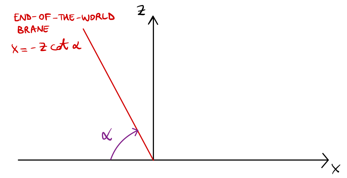
Figure 1: Schematic set-up of the AdS/BCFT model. We represent a section at constant time and represent the end-of-the-world brane as the red hypersurface defined by $x=-z\cot\alpha.$

2.3 Gravitational action with null boundaries

In order to evaluate the gravitational action associated to a subsystem on the boundary, we discuss the contributions coming from null boundaries, following [11]. The total on-shell action is

$$I_{\rm tot} =\frac{1}{16\pi G}\int_{\rm WDW\cap EW}d^{d+1}x\,\sqrt{-g}\left(R+\frac{2}{L^{2}}\right)$$ (2.12)

$$+\frac{\varepsilon_{t,s}}{8\pi G}\int_{\mathcal{B}_{t,s}}d^{d}x\,\sqrt{|h|}\,K+\frac{\varepsilon_{n}}{8\pi G}\int_{\mathcal{B}_{n}}d\lambda\,d^{d-1}x\,\sqrt{\gamma}\,\kappa$$

$$+\frac{\varepsilon_{\eta}}{8\pi G}\int_{\mathcal{J}_{t,s}}d^{d-1}x\,\sqrt{\gamma}\,\eta+\frac{\varepsilon_{\mathfrak{a}}}{8\pi G}\int_{\mathcal{J}_{n}}d^{d-1}x\,\sqrt{\gamma}\,\mathfrak{a}$$

$$+\frac{1}{8\pi G}\int_{\mathcal{B}_{n}}d\lambda\,d^{d-1}x\,\sqrt{\gamma}\,\Theta\log|\tilde{L}\Theta|\,,$$

where $d=2$ in the cases considered in the present work. We comment on each term:

• The first line contains the bulk term, i.e. the Einsten-Hilbert action with cosmological constant, evaluated in the intersection between the WDW patch and the EW. For the Janus geometry, the bulk term also includes the kinetic part of the dilaton field, see eq. (2.1).

• The second line contains codimension-one boundary terms which make the variational problem well-defined. The first contribution refers to timelike or spacelike surfaces $\mathcal{B}_{t,s}$ and it is the Gibbons-Hawking-York (GHY) term, containing the determinant of the induced metric $h$ and the trace $K$ of the extrinsic curvature. In the case of the AdS/BCFT model, this term is supplemented by a tension term involving the end-of-the-world brane, see eq. (2.10). The second term is evaluated on the null boundaries $\mathcal{B}_{n}$ and involves the integration along the parameter $\lambda$ describing a congruence of null geodesics generating the surface and the integration along the remaining $(d-1)$ orthogonal directions with induced metric $\gamma.$ The parameter $\kappa$ is defined by the geodesic equation

  $$k^{\nu}D_{\nu}k^{\mu}=\kappa\,k^{\mu}\,.$$ (2.13)

  If the parameter $\lambda$ is affine, $\kappa$ identically vanishes. The prefactors $\varepsilon_{t,s}$ and $\varepsilon_{n}$ (referring to timelike/spacelike and null surfaces, respectively) take the values $\pm 1$ depending on the orientation of the normals to the hypersurfaces $\mathcal{B}_{t,s}$ or $\mathcal{B}_{n}$ of interest.

• The third line contains joint terms, which are codimension-two surfaces found at the intersection of the previous codimension-one boundary terms. When there is at least a timelike or spacelike surface, they involve the boost parameter $\eta,$ while in the purely null case they contain a scalar product of the corresponding null normals, here denoted with $\mathfrak{a}.$ We will be more explicit about the expressions of the integrands when doing the actual computations of this work.

• The last line is a counterterm which must be included on null boundaries to restore reparametrization invariance, which is broken by the terms in the second and third lines. This introduces an extra scale $\tilde{L}$. This term involves the expansion parameter $\Theta$ along the null geodesics, which will be introduced in eq. (3.7).

Since the geometries under consideration are static and do not present causally disconnected boundaries, it is not restrictive to consider the case where the time on both boundaries is vanishing. In order to set up the actual computation, we need to determine the WDW patch and the EW, which both require to analyze null geodesics in the spacetime of interest. Before doing that, we comment on the regularization prescriptions that will be used throughout the paper.

2.4 Regularization prescriptions for UV divergences

We are interested in the computation of the UV divergences of the subregion action for theories with defects. These kinds of geometries can be described by performing an $\mathrm{AdS}_{d}$ slicing of asymptotically $\mathrm{AdS}_{d+1}$ space to obtain a metric in the form [69]

$$ds^{2}=L^{2}\left(A^{2}(y)ds^{2}_{\mathrm{AdS}_{d}}+\rho^{2}(y)dy^{2}\right)\,,$$ (2.14)

where $y$ is a non-compact coordinate such that when $y\rightarrow\pm\infty$

$$A(y)\rightarrow\frac{L_{\pm}}{2}e^{\pm y\pm c_{\pm}}\,,\qquad\rho(y)\rightarrow 1\,,$$ (2.15)

where $L_{\pm}$ and $c_{\pm}$ are constants. We parametrize the $\mathrm{AdS}_{d}$ slices using Poincaré coordinates

$$ds^{2}_{\mathrm{AdS}_{d}}=\frac{1}{z^{2}}\left(dz^{2}-dt^{2}+d\vec{x}^{2}_{d-2}\right)\,,$$ (2.16)

where $(t,z)$ are the time and radial coordinates on each slice and $\vec{x}$ collects all the other orthogonal directions.

Three different regularisation prescriptions have been used the literature [69, 70, 71]:

• The Fefferman-Graham (FG) regularization relies on performing a FG expansion of the metric to select a radial direction $\xi$ for the asymptotic AdS_d+1 region in Poincaré coordinates, and introducing a UV cutoff by cutting the spacetime with a surface located at $\xi=\delta.$ The metric in FG form reads

  $$ds^{2}=\frac{L^{2}}{\xi^{2}}\left[d\xi^{2}+g_{1}(\xi/\eta)\,\left(-dt^{2}+d\vec{x}^{2}\right)+g_{2}(\xi/\eta)\,d\eta^{2}\right]\,,$$ (2.17)

  where $\xi$ is a radial coordinate for the asymptotic AdS region in Poincaré coordinates, $\eta$ is the boundary direction orthogonal to the defect, and $g_{1},g_{2}$ are two appropriate functions, such that the original metric (2.14) with slicing (2.16) is equivalent to (2.17) with a suitable change of coordinates $(z,y)\rightarrow(\xi,\eta).$ In the region $\xi\gg\eta$, the FG expansion breaks down because the coordinates $\xi$ and $\eta$ are not well defined [73]. This problem can be solved by introducing a continuous curve which interpolates between the right and left patches of the defect [69].

• In the single cutoff regularization [70] the arbitrary interpolation curve is replaced by a cutoff on the minimal value of the $z$ coordinate such that

  $$\delta=\frac{z}{A(y)}\,,\qquad z_{\rm min}=\delta\,\underset{y\in\mathbb{R}}{\mathrm{min}}\,[A(y)]\,.$$ (2.18)

  The physical quantities are then expanded in series around $\delta=0.$

• The double cutoff regularization [71] introduces two different cutoffs for each of the directions $(y,z)$. The first cutoff is directly imposed on the $\mathrm{AdS}_{d}$ slicing at $z=\delta.$ The second cutoff regularizes the divergences of $A(y)$ at infinity. This can be achieved by restricting the $y$ domain up to a maximum value $y^{*}$, defined by

  $$A(y^{*})=\frac{1}{\varepsilon}\,.$$ (2.19)

  While the $\delta$ cutoff has physical relevance since it regularizes the intrinsic contributions from the defect, the $\varepsilon$ cutoff is only a mathematical artifact introduced at intermediate steps. Observables which are intrinsic to the defect must be $\varepsilon$-independent after the subtraction of the vacuum solution.

The advantage of both the FG and the single cutoff regularizations is the introduction of only one regulator; the drawback is that integrals along different coordinates are nested. From a technical point of view, it is simpler to consider the double cutoff regularization. For volume complexity, we checked [68, 74] that all the three methods only differ by finite parts, while we expect universal contributions to appear in logarithmically divergent terms. We then choose to evaluate the action complexity with the double cutoff method, since the universal behaviour is not influenced by the regularization scheme.

The previous discussion applies in particular to the case of the Janus AdS geometry and will be used in section 3.3. The case of the AdS/BCFT model is simpler, because the spacetime is empty AdS space with the addition of an end-of-the-world brane. While it is still possible to employ the parametrization (2.14), it is simpler to work using three-dimensional Poincaré coordinates including a UV regulator cutting the spacetime with the surface $z=\delta,$ without any need for a second parameter $\varepsilon.$ This choice will be used for the computations in section 4.

The three regularization procedures discussed above do not represent the only ambiguities involving the computation of the action. It is also possible to define the WDW patch surfaces in two different ways [12], depicted in Fig. 2:

• Regularization A amounts to build the WDW patch starting from the true boundary located at $z=0,$ and cut the spacetime with a surface located at $z=\delta.$

• Regularization B corresponds to the null geodesics delimiting the WDW patch to directly start from the cutoff surface surface located at $z=\delta.$

The same ambiguity arises for the Ryu-Takayanagi (RT) surface.

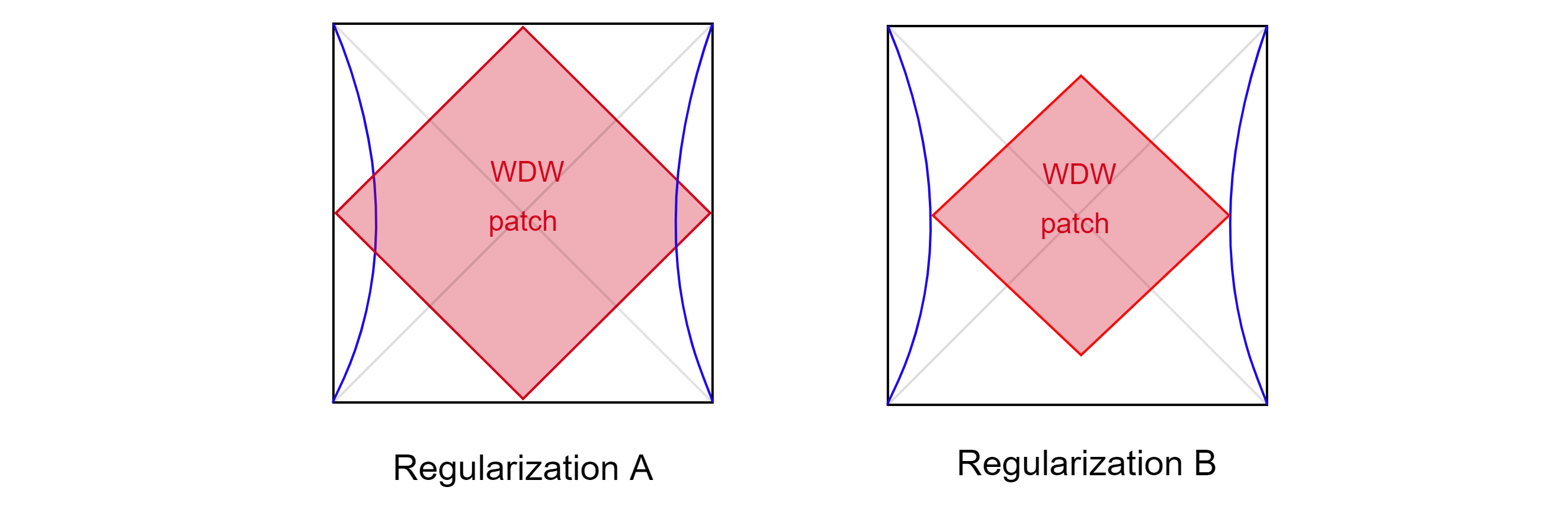
Figure 2: The two regularizations of the WDW patch introduced in [12]. In the picture it is represented the case of a black hole in asymptotically AdS spacetime.

In this paper we will work with regularization A. The divergences of regulatization B are related to the ones of regularization A by another counterterm that can be introduced on the cutoff at the boundary [75, 76], in the spirit of holographic renormalization [77, 78, 79, 80]. We will check that in our case such a counterterm is finite (see Appendix C).

3 Subregion complexity in the Janus AdS₃ geometry

In this section we perform the computation of the subregion action complexity in the Janus AdS₃ spacetime. In section 3.1 we review some background material on null surfaces and on the properties of null geodesics under conformal transformations. In section 3.2 we find the integration domain for the action. In section 3.3 we perform the actual calculation.

3.1 Null surfaces, geodesic congruencies and conformal rescalings

The boundary of the integration domain of the action will involve many null hypersurfaces. Let us review a few useful properties, following [81]. We consider a null hypersurface $\Sigma$ selected by an appropriate restriction on the coordinates $x^{\mu}$ of spacetime

$$\Phi(x^{\mu})=0\,,$$ (3.1)

where $\Phi$ is a scalar function increasing towards the future. The normal one-form $k_{\mu}$ to $\Sigma$, defined by

$$k_{\mu}=-\alpha\partial_{\mu}\Phi\,,$$ (3.2)

is by construction null $k^{\mu}k_{\mu}=0$ and also tangent to $\Sigma$. Here $\alpha>0$ is a constant prefactor, such that the corresponding vector $k^{\mu}$ is future-oriented.

Moreover, the vector field $k^{\mu}$ satisfies the geodesic equation

$$k^{\nu}D_{\nu}k^{\mu}=\kappa\,k^{\mu}\,,$$ (3.3)

where $\kappa$ is a spacetime scalar which vanishes for affine parameterisations.

We can in general parameterize a null hypersurface as a congruence of null geodesics. Besides using an implicit expression of kind (3.1) an alternative way to parametrize a null hypersurface is through the expression $X^{\mu}=X^{\mu}(\lambda,\theta^{A})$ with the requirements that the parameter $\lambda$ moves along a single generator in the congruence of null geodesics, and the parameters $\theta^{A}$ are constant on each null generator spanning the hypersurface. We define then the tangent vectors along the hypersurface to be

$$k^{\mu}\equiv\frac{dX^{\mu}}{d\lambda}\,,\qquad e^{\mu}_{A}\equiv\frac{dX^{\mu}}{d\theta^{A}}\,,$$ (3.4)

where $k^{\mu}$ is the null tangent vector and $e^{\mu}_{A}$ is a spacelike vector, defined in such a way that it is orthogonal to $k^{\mu}$, i.e.

$$k^{\mu}e^{A}_{\mu}=0\,.$$ (3.5)

The normal $k^{\mu}$ satisfies eq. (3.3) where $\kappa$ is a function of $\lambda$. The vectors $e^{\mu}_{A}$ define the induced metric

$$\gamma_{AB}=g_{\mu\nu}e^{\mu}_{A}e^{\nu}_{B}\,.$$ (3.6)

The expansion parameter along the congruence of null geodesics is given by

$$\Theta=\frac{1}{\sqrt{\gamma}}\frac{d\sqrt{\gamma}}{d\lambda}\,,$$ (3.7)

where $\gamma$ is the determinant of $\gamma_{AB}$.

In order to determine the null hypersurface in Janus, it will be convenient to perform a conformal rescaling. Let us review a few basic properties [82, 83] Consider two metrics $g$ and $\tilde{g}$ related by a conformal transformation

$$\tilde{g}_{\mu\nu}(x^{\prime})=\Omega(x)^{2}\,g_{\mu\nu}(x)\,.$$ (3.8)

Under this map the causal structure of the spacetime is preserved. While in general the two metrics have different spacelike and timelike geodesics, the null geodesics are the same. However, the affine parameterization condition of these geodesics in general is not preserved under (3.8).

As a matter of fact, starting from an affine parameterization for the geodesics of the metric $g$, i.e.

$$k^{\nu}D_{\nu}k^{\mu}=0\,,$$ (3.9)

under the conformal transformation (3.8) the equation (3.9) becomes

$$k^{\nu}\tilde{D}_{\nu}k^{\mu}=\kappa\,k^{\mu}\,,\qquad\kappa=\frac{2}{\Omega}\frac{d\Omega}{d\lambda}\,.$$ (3.10)

We can think of $\kappa(\lambda)$ as the measure of the failure of $\lambda$ to be an affine parameter.

3.2 Null boundaries in the Janus AdS₃ geometry

Using a conformal transformation with

$$\Omega^{2}=L^{2}\frac{f(\mu)}{z^{2}}\;.$$ (3.11)

we can write the Janus metric (2.2) as

$$d\tilde{s}^{2}=\Omega^{2}\,ds^{2}\,,\qquad ds^{2}=-dt^{2}+dz^{2}+z^{2}d\mu^{2}$$ (3.12)

where $ds^{2}$ is the flat spacetime metric in polar coordinates. We proceed to study the null congruence of geodesics delimiting the WDW patch and the EW.

WDW patch. By going to cartesian coordinates

$$X=z\sin\mu\,,\qquad Y=z\cos\mu\,,$$ (3.13)

we bring the metric to the form $ds^{2}=-dt^{2}+dX^{2}+dY^{2}$. In these coordinates, the two-dimensional plane specified by

$$g(t,X,Y)=a\,X+b\,Y+c\,t=0\,,\qquad c=\pm\sqrt{a^{2}+b^{2}}\,,$$ (3.14)

is a null surface. From now on we will specialize to the case of $c<0,$ in view of the parametrization of the part at positive time of the WDW patch.

From the general result that null geodesics are invariant under conformal transformations of the metric, it follows that eq. (3.14) specifies a null surface also in the Janus $\mathrm{AdS}_{3}$ background. In polar coordinates, it reads

$$g(t,\mu,z)=a\,z\sin\mu+b\,z\cos\mu+c\,t=0\,.$$ (3.15)

Let us first consider the WDW patch anchored at the right boundary $\mu=\mu_{0}.$ In order to impose that this null surface is part of the boundary of the WDW patch in the regularization A, we enforce that at $t=0,$ the angular coordinate is $\mu=\mu_{0}.$ This condition determines

$$\tan\mu_{0}=-\frac{b}{a}\,.$$ (3.16)

Therefore we conclude that the null boundary of the WDW patch is described by the equations

$$t_{\rm WDW}(\mu,z)=z\sin\left(\mu_{0}-\mu\right)\,,$$ (3.17)

where we used as a working assumption that $\mu_{0}\in[\pi/2,\pi].$ Using eq. (2.5), this implies

$$\gamma\leq\gamma_{0}\approx 0.704\,.$$ (3.18)

For simplicity, we will restrict to the case $\gamma\in[0,\gamma_{0}]$. In the case $\gamma\in\left(\gamma_{0},\frac{1}{\sqrt{2}}\right),$ the geometry of the WDW patch changes.

We can then describe the boundary of the WDW patch as

$$X^{\mu}_{\rm WDW}=\left(t_{\rm WDW}(\mu,z),\mu,z\right)\,.$$ (3.19)

Since the spacetime is three-dimensional, there is only one coordinate $\theta$ entering eq. (3.4), i.e.

$$k^{\mu}_{R}=\frac{dX^{\mu}_{\rm WDW}}{d\lambda}\,,\qquad e^{\mu}_{R}=\frac{dX^{\mu}_{\rm WDW}}{d\theta}\,.$$ (3.20)

We should also impose that the orthogonality condition (3.5) holds. The affine parameterization is not convenient for the calculation. It turns out that a convenient choice is

$$\lambda=-\frac{z}{\alpha}\sin\left(\mu_{0}-\mu\right)\,,\qquad\theta=-\log\left(z\cos\left(\mu_{0}-\mu\right)\right)\,,$$ (3.21)

where $\alpha>0$ parametrizes the ambiguity in the normalization of a null vector. With this choice, eq. (3.20) takes the form

$$k^{\mu}_{R}=-\alpha\left(1,-\frac{\cos\left(\mu_{0}-\mu\right)}{z},\sin\left(\mu_{0}-\mu\right)\right)\,,$$ (3.22)

$$e^{\mu}_{R}=-\left(0,\frac{1}{2}\sin\left(2(\mu_{0}-\mu)\right),z\cos^{2}\left(\mu_{0}-\mu\right)\right)\,,$$ (3.23)

The induced metric $\gamma$ (which is a number because it is a $1$ by $1$ matrix), the expansion parameter $\Theta$ and the scalar $\kappa$ are given by:

$$\gamma_{\rm WDW} = L^{2}f(\mu)\cos^{2}\left(\mu_{0}-\mu\right)\,,$$

$$\Theta_{\rm WDW} = \alpha\,\left[\frac{\sin\left(\mu_{0}-\mu\right)}{z}+\frac{\cos\left(\mu_{0}-\mu\right)}{2z}\frac{f^{\prime}(\mu)}{f(\mu)}\right]\,,$$

$$\kappa_{\rm WDW}(\lambda) = 2\Theta_{\rm WDW}\,.$$ (3.24)

The boundary of the WDW patch anchored at the left boundary $L$ (placed at $\mu=-\mu_{0}$) can be treated in an analog way, obtaining

$$X^{\mu}_{\rm WDW,L}=\left(z\sin\left(\mu+\mu_{0}\right),\mu,z\right)\,.$$ (3.25)

The corresponding parameterization is

$$\lambda=-\frac{1}{\alpha}\,z\sin\left(\mu+\mu_{0}\right)\,,\qquad\theta=-\log\left(z\cos\left(\mu+\mu_{0}\right)\right)\,,$$ (3.26)

which gives the following vectors

$$k^{\mu}_{L} = -\alpha\left(1,\frac{\cos\left(\mu+\mu_{0}\right)}{z},\sin\left(\mu+\mu_{0}\right)\right)\,,$$

$$e^{\mu}_{L} = \left(0,\frac{1}{2}\sin\left(2(\mu+\mu_{0})\right),-z\cos^{2}\left(\mu+\mu_{0}\right)\right)\,,$$ (3.27)

and the following geometric data

$$\gamma_{\rm WDW,L} = L^{2}f(\mu)\cos^{2}\left(\mu+\mu_{0}\right)\,,$$

$$\Theta_{\rm WDW,L} = \alpha\,\left[\frac{\sin\left(\mu+\mu_{0}\right)}{z}-\frac{\cos\left(\mu+\mu_{0}\right)}{2z}\frac{f^{\prime}(\mu)}{f(\mu)}\right]\,,$$

$$\kappa_{\rm WDW,L}(\lambda) = 2\Theta_{\rm WDW,L}\,.$$ (3.28)

For future convenience, we write the normal to the left and right side of the WDW patch as one-forms

$$\mathbf{k}_{R}=\alpha\,\frac{L^{2}f(\mu)}{z^{2}}\left(dt+z\cos\left(\mu_{0}-\mu\right)d\mu-\sin\left(\mu_{0}-\mu\right)dz\right)\,,$$

$$\mathbf{k}_{L}=\alpha\,\frac{L^{2}f(\mu)}{z^{2}}\left(dt-z\cos\left(\mu+\mu_{0}\right)d\mu-\sin\left(\mu+\mu_{0}\right)dz\right)\,.$$ (3.29)

Entanglement wedge. Since the Janus metric is conformally equivalent to $2+1$ dimensional flat spacetime, the two spaces share the same null geodesics, in particular the lightcones at constant $\mu$

$$z=\pm t\pm c\,.$$ (3.30)

Here the constant $c$ will be determined by suitable boundary conditions. We will show that the geodesics (3.30) define the boundary of the EW.

The Ryu-Takayanagi (RT) surface anchored at the boundary [84] is described by the equation

$$z_{\rm RT}=l/2$$ (3.31)

for an interval of length $l$ located symmetrically along $\mu$ on the surface at constant time $t=0.$ By imposing that the curves at constant $\mu$ given in eq. (3.30) pass through the RT surface, we determine that the null boundary of the EW is

$$t_{\rm EW}=\frac{l}{2}-z\,,$$ (3.32)

where we are restricting the solution to the part with positive time coordinate. This expression holds both in empty AdS space and in the Janus background.

It is convenient to work in the affine parametrization. The Langrangian which describes affinely parametrized geodesics is of the form

$$\mathcal{L}=\Omega^{2}\left(-\dot{t}^{2}+\dot{z}^{2}+z^{2}\dot{\mu}^{2}\right)\,,$$ (3.33)

where dot denotes derivative with respect to the affine parameter. The equations of motion give the following tangent vector for the null geodesics with constant $\mu$

$$w^{\mu}=\beta\,(\dot{t},\dot{z},0)=\beta\frac{1}{\Omega^{2}}(-1,1,0)\,,$$ (3.34)

where $\beta$ is an arbitrary constant. Lowering the indices, we get the one-form

$$\mathbf{w}=\beta\left(dt+dz\right)\,.$$ (3.35)

Note that the dependence on the conformal factor disappears on the form $\mathbf{w}$. Such one-form is orthogonal at the boundary to the curve parametrizing the RT surface, i.e.

$$w_{\mu}\frac{dX^{\mu}_{\rm RT}}{d\lambda}\Big{|}_{\rm bdy}=0\,,$$ (3.36)

This shows that the congruence of null geodesics (3.32) describes indeed the null boundary of the EW. As anticipated, the parametrization is affine and therefore $\kappa_{\rm EW}=0$. From eq. (3.7), we find that the expansion parameter vanishes $\Theta_{\rm EW}=0$, as expected on general grounds since the EW is delimited by an extremal surface [85].

Intersection curve. In view of the computation of the gravitational action, we need to determine the intersection curve between the WDW patch and the EW. It is sufficient for symmetry reasons to focus on the region with positive $(t,\mu).$ By equating the hypersurfaces defined in eq. (3.17) and eq. (3.32), we obtain the following curve

$$z_{\rm int}(\mu)=\frac{l}{2}\frac{1}{\sin\left(\mu_{0}-\mu\right)+1}\,.$$ (3.37)

A picture of the WDW patch, the EW and their intersecton curve in $(t,X,Y)$ coordinates is shown in Fig. 3.

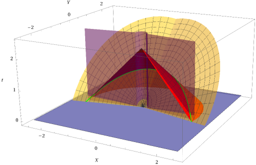
Figure 3: A pictorial representation of the null boundaries of the WDW patch (light orange surfaces), of the entanglement wedge (red), and the intersection curve $z_{\rm int}(\mu)$ between them (green). The blue plane restricts the integration region to $t\geq 0$ only. The purple transparent region represents the cutoff surfaces located at $z=\delta$ and $\mu=\pm\mu^{*}(\varepsilon).$ The diagram corresponds to the choice $\gamma=0.5.$

3.3 Computation of the action

We are now ready to compute the gravitational action (2.12) in the Janus AdS₃ background using the double cutoff prescription. The equivalent of eq. (2.19) for this case is

$$\sqrt{f(y^{*})}=\frac{1}{\varepsilon}\,.$$ (3.38)

This equation determines a value of $y^{*}(\varepsilon)$ which delimits the corresponding integration

$$y^{*}(\varepsilon)=\frac{1}{2}\,\mathrm{arccosh}\left(\frac{\frac{2}{\varepsilon^{2}}-1}{\sqrt{1-2\gamma^{2}}}\right)\,.$$ (3.39)

We can express this result in terms of the $\mu$ coordinates by means of the change of variables

$$\tanh y=\mathrm{sn}\left(\alpha_{+}\mu|m\right)\,,$$ (3.40)

which infinitesimally corresponds to eq. (2.6) and where we are using the definitions (2.5). A derivation of eq. (3.40) is provided in in eq. (A.9). The corresponding value of the cutoff in the $\mu$ variable, such that $\sqrt{f(\mu^{*}(\varepsilon))}=\varepsilon^{-1}$, can be obtained by combining eqs. (3.39) and  (3.40).

We compute the subregion action term by term. Our general strategy will be the following: we will evaluate explicitly the integrations over $(t,z),$ while we will collect all the integrands in the $\mu$ variables, and extract their divergences at the very end of the calculation.

3.3.1 Bulk term

The bulk term reads

$$I_{\mathcal{B}}=\frac{1}{16\pi G}\int_{\rm WDW\cap EW}d^{3}x\,\sqrt{-g}\,\mathcal{L}\,,\qquad\mathcal{L}=R+\frac{2}{L^{2}}-g^{\mu\nu}\partial_{\mu}\phi\partial_{\nu}\phi\,,$$ (3.41)

where $R$ is the Ricci scalar of the metric (2.6) with profile function $f$ and dilaton solution given in eq. (2.7). It is important to remark that the presence of the defect is responsible for the backreaction of the original vacuum $\mathrm{AdS}_{3}$ spacetime, which leads to a different value of the Ricci scalar than empty AdS. However, the addition of a kinetic term for the dilaton gives a simple on-shell action which reads

$$\mathcal{L}=-\frac{4}{L^{2}}\,.$$ (3.42)

The intersection curve between the null boundaries of the WDW patch and the EW naturally splits the integration region in two parts:

$$I_{\mathcal{B}}=I_{\mathcal{B}}^{1}+I_{\mathcal{B}}^{2}\,,$$ (3.43)

where

$$I_{\mathcal{B}}^{1} = -\frac{L}{\pi G}\int_{0}^{\mu^{*}(\varepsilon)}d\mu\int_{\delta}^{z_{\rm int}(\mu)}dz\int_{0}^{t_{\rm WDW}(\mu,z)}dt\,\frac{f(\mu)^{3/2}}{z^{2}}\,,$$

$$I_{\mathcal{B}}^{2} = -\frac{L}{\pi G}\int_{0}^{\mu^{*}(\varepsilon)}d\mu\int_{z_{\rm int}(\mu)}^{z_{\rm RT}}dz\int_{0}^{t_{\rm EW}(z)}dt\,\frac{f(\mu)^{3/2}}{z^{2}}\,.$$ (3.44)

We introduced a symmetry factor of 4 coming from the integrations along $(t,\mu).$ A direct evaluation of the integrals over $(t,z)$ brings to the result

$$I_{\mathcal{B}}=\frac{L}{\pi G}\int_{0}^{\mu^{*}(\varepsilon)}d\mu\,f(\mu)^{3/2}\,\biggl{\{}\left(\sin\left(\mu_{0}-\mu\right)+1\right)\log\left[\sin\left(\mu_{0}-\mu\right)+1\right]\biggr{.}$$

$$\biggl{.}+\sin\left(\mu_{0}-\mu\right)\left[\log\left(\frac{2\delta}{l}\right)-1\right]\biggr{\}}\,.$$ (3.45)

3.3.2 GHY term

The regularization prescription A in Fig. 2 requires to evaluate the GHY term

$$I_{\rm GHY}=\frac{\varepsilon_{t,s}}{8\pi G}\int_{\mathcal{B}_{t,s}}d^{2}x\,\sqrt{|h|}\,K\,,$$ (3.46)

at the cutoff surfaces $z=\delta$ and $\mu=\pm\mu^{*}(\varepsilon).$ In eq. (3.46) $K$ is the trace of the extrinsic curvature, $h$ the determinant of the induced metric, and $\varepsilon_{t,s}=\pm 1$ if the surface of interest ${\mathcal{B}_{t,s}}$ is timelike or spacelike, respectively.

Cutoff surface located at $z=\delta$. The unit normal vector $n^{\mu}$ to the cutoff surface located at $z=\delta$ is given by

$$n_{1}^{\mu}=-\frac{z}{L\sqrt{f(\mu)}}\left(0,0,1\right)\,,$$ (3.47)

the minus sign being chosen in such a way that it is outward-directed from the region of interest for the computation of the action. The determinant of the induced metric and the trace of the extrinsic curvature are

$$\sqrt{-h}=L^{2}\,\frac{f(\mu)}{z}\,,\qquad K=D_{\mu}n_{1}^{\mu}=\frac{1}{L\sqrt{f(\mu)}}\,.$$ (3.48)

In principle, one would expect to split the integration region according to the intersection curve $z_{\rm int}(\mu)$ in eq. (3.37) between the null boundaries of the WDW patch and of the EW. However, a choice of a small enough value of $\delta$ always allows to keep the entire cutoff surface inside the region where the WDW patch sits below the EW, since

$$z_{\rm int}(\mu)=\frac{l}{2}\frac{1}{\sin\left(\mu_{0}-\mu\right)+1}\geq\frac{l}{4}\,.$$ (3.49)

For this reason, the GHY term reads

$$I^{\delta}_{\rm GHY}=\frac{L}{2\pi G}\int_{0}^{\mu^{*}(\varepsilon)}d\mu\int_{0}^{t_{\rm WDW}(\delta,\mu)}dt\,\frac{\sqrt{f(\mu)}}{\delta}\,,$$ (3.50)

where we put a symmetry factor of 4 (there is a factor of 2 from each of the two integrations). Performing the first integration, we find

$$I^{\delta}_{\rm GHY}=\frac{L}{2\pi G}\int_{0}^{\mu^{*}(\varepsilon)}d\mu\,\sqrt{f(\mu)}\,\sin\left(\mu_{0}-\mu\right)\,.$$ (3.51)

Cutoff surface located at $\mu=\mu^{*}(\varepsilon)$. The outward-directed normal to the cutoff surface located at $\mu=\mu^{*}(\varepsilon)$ is given by

$$n_{2}^{\mu}=\frac{1}{L\sqrt{f(\mu)}}(0,1,0)\,,$$ (3.52)

and the determinant of the induced metric and the trace of the extrinsic curvature are

$$\sqrt{-h}=L^{2}\frac{f(\mu)}{z^{2}}\,,\qquad K=D_{\mu}n^{\mu}_{2}=\frac{1}{L}\frac{f^{\prime}(\mu)}{f(\mu)^{3/2}}\,.$$ (3.53)

In this case, the surface $\mu=\mu^{*}(\varepsilon)$ cuts both the WDW patch and the EW; for this reason, the GHY term decomposes into two parts determined by the intersection curve in eq. (3.37). These codimension-one boundary terms are given by

$$I^{\varepsilon}_{\rm GHY}=I^{\varepsilon}_{\rm GHY,1}+I^{\varepsilon}_{\rm GHY,2}\,,$$ (3.54)

where

$$I^{\varepsilon}_{\rm GHY,1} = \frac{L}{2\pi G}\int_{\delta}^{z_{\rm int}(\mu^{*}(\varepsilon))}dz\int_{0}^{t_{\rm WDW}(z,\mu^{*}(\varepsilon))}dt\,\frac{f^{\prime}(\mu)}{z^{2}\,\sqrt{f(\mu)}}\Big{|}_{\mu=\mu^{*}(\varepsilon)}$$

$$I^{\varepsilon}_{\rm GHY,2} = \frac{L}{2\pi G}\int_{z_{\rm int}(\mu^{*}(\varepsilon))}^{z_{\rm RT}}dz\int_{0}^{t_{\rm EW}(z)}dt\,\frac{f^{\prime}(\mu)}{z^{2}\,\sqrt{f(\mu)}}\Big{|}_{\mu=\mu^{*}(\varepsilon)}$$ (3.55)

In these integratons, we already put the symmetry factor of 4 (one factor of 2 comes from the integration along $t,$ while the other factor of 2 arises because we also account for the cutoff surface located at $\mu=-\mu^{*}(\varepsilon)$ by symmetry reasons). Both these integrations can be performed explicitly, and further simplifications occur by using properties of the elliptic functions to find

$$f\left(\mu^{*}(\varepsilon)\right)=\frac{1}{\varepsilon^{2}}\,,\qquad\frac{df}{d\mu}\Big{|}_{\mu=\mu^{*}(\varepsilon)}=\frac{2}{\varepsilon^{3}}\sqrt{\left(1-\alpha_{+}^{2}\varepsilon^{2}\right)\left(1-m\alpha_{+}^{2}\varepsilon^{2}\right)}\,.$$ (3.56)

Employing these identities and solving the integrals, we find

$$I^{\varepsilon}_{\rm GHY}= \frac{L}{\pi G\varepsilon^{2}}\sqrt{\left(1-\alpha_{+}^{2}\varepsilon^{2}\right)\left(1-m\alpha_{+}^{2}\varepsilon^{2}\right)}\,\left\{\sin\left(\mu_{0}-\mu^{*}(\varepsilon)\right)\left[1-\log\left(\frac{2\delta}{l}\right)\right]\right.$$ (3.57)

$$\biggl{.}-\left[\sin\left(\mu_{0}-\mu^{*}(\varepsilon)\right)+1\right]\,\log\left[\sin\left(\mu_{0}-\mu^{*}(\varepsilon)\right)+1\right]\biggr{\}}\,.$$

3.3.3 Null boundary terms

The contribution due to null boundaries is of the following form

$$I_{\mathcal{N}}=\frac{\varepsilon_{n}}{8\pi G}\int_{\mathcal{B}_{n}}d\lambda d\theta\,\,\sqrt{\gamma}\,\kappa(\lambda)\,,$$ (3.58)

where $\varepsilon_{n}=\pm 1$ depends on the orientation of the null normal to the surface, $\lambda$ is a parameter along the congruence of geodesics, $\gamma$ is the induced metric along the $\theta$ direction and $\kappa(\lambda)$ is defined in the geodesic equation (3.3).

WDW patch. Using the parametrization in eq. (3.21), the WDW patch is not affinely parametrized and therefore we need to evaluate the following integral:

$$I^{\rm WDW}_{\mathcal{N}}=\frac{\alpha L}{4\pi G}\iint d\lambda\,d\theta\,\,\left[\frac{\sin\left(\mu_{0}-\mu\right)}{z}+\frac{\cos\left(\mu_{0}-\mu\right)}{2z}\frac{f^{\prime}(\mu)}{f(\mu)}\right]\,\sqrt{f(\mu)}\left|\cos\left(\mu_{0}-\mu\right)\right|\,.$$ (3.59)

We take $\varepsilon_{n}=1$ because the spacetime region under consideration lies in the past of the null boundary of the WDW patch [11].

We change integration variables from $(\lambda,\theta)$ to $(\mu,z)$ using the Jacobian determinant

$$J=\frac{1}{\alpha\,\cos\left(\mu_{0}-\mu\right)}\,,$$ (3.60)

leading to the following form:

$$I^{\rm WDW}_{\mathcal{N}}=\frac{L}{\pi G}\int_{0}^{\mu^{*}(\varepsilon)}d\mu\int_{\delta}^{z_{\rm int}(\mu)}dz\,\sqrt{f(\mu)}\left[\frac{\sin\left(\mu_{0}-\mu\right)}{z}+\frac{\cos\left(\mu_{0}-\mu\right)}{2z}\frac{f^{\prime}(\mu)}{f(\mu)}\right]\,.$$ (3.61)

We put a symmetry factor of 4 to take into account both the region at negative time and the analog boundary term associated to the WDW patch anchored at the boundary $\mu=-\mu_{0}.$ An explicit evaluation gives

$$I^{\rm WDW}_{\mathcal{N}} =\frac{L}{\pi G}\int_{0}^{\mu^{*}(\varepsilon)}d\mu\,\left[\sqrt{f(\mu)}\,\sin\left(\mu_{0}-\mu\right)+\frac{f^{\prime}(\mu)}{2\sqrt{f(\mu)}}\cos\left(\mu_{0}-\mu\right)\right]$$ (3.62)

$$\times\left[\log\left(\frac{l}{2\delta}\right)-\log\left(1+\sin\left(\mu_{0}-\mu\right)\right)\right]\,.$$

Entanglement wedge. We use an affine parameterization for the boundaries of EW, so eq. (3.58) vanishes.

3.3.4 Joint terms

The typical structure of a codimension-two joint [11] term reads

$$I_{\mathcal{J}_{n}}=\frac{\varepsilon_{\mathfrak{a}}}{8\pi G}\int_{\mathcal{J}_{n}}d^{d-1}x\,\sqrt{\gamma}\,\mathfrak{a}\,,$$ (3.63)

for the case where at least one null boundary is included, as it will always be the case in the following computation. The expression of $\mathfrak{a}$ will be specified for each case and involve appropriate scalar products of the null normals. The coefficients $\varepsilon_{\eta},\varepsilon_{\mathfrak{a}}=\pm 1$ depend on the orientations of the normal one-forms, while $\gamma$ is the determinant of the induced metric along the codimension-two joint.

Joint between the cutoff $z=\delta$ and the WDW patch. This joint involves the timelike surface $z=\delta$ and the null boundary of the WDW patch, therefore it reads

$$I_{\mathcal{J}}^{\rm\delta,WDW}=\frac{\varepsilon_{\eta}}{2\pi G}\int_{0}^{\mu^{*}(\varepsilon)}d\mu\,\sqrt{\gamma}\,\log|\mathbf{k}_{R}\cdot\mathbf{n}_{1}|\,,$$ (3.64)

where $\mathbf{k}_{R}$ and $\mathbf{n}_{1}$ were defined in eq. (3.2) and (3.47), respectively.

We put a symmetry factor of 2 for the integration along $\mu,$ and another factor of 2 due to the presence of two joints of this kind, at positive and negative times. We determine the sign $\varepsilon_{\eta}$ according to [11]: with respect to the null boundary of the WDW patch, the joint is a past boundary and the outward direction is a future one. Therefore we get the sign

$$\varepsilon_{\eta}=-1.$$ (3.65)

The induced metric is determined by imposing that the joint is located at constant $z=\delta,$ and that the intersection between such cutoff surface and the null boundary of the WDW patch is given by

$$t_{\rm WDW}(\mu,\delta)=\delta\sin\left(\mu_{0}-\mu\right)\,.$$ (3.66)

In this way we get

$$ds^{2}_{\rm ind}=L^{2}f(\mu)\left[1-\frac{1}{z^{2}}\left(\frac{dt_{\rm WDW}(\mu,\delta)}{d\mu}\right)^{2}\right]d\mu^{2}\,,$$ (3.67)

with induced metric determinant

$$\sqrt{\gamma}=L\sqrt{f(\mu)}\sin\left(\mu_{0}-\mu\right)\,.$$ (3.68)

The integrand reads

$$\log|\mathbf{k}_{R}\cdot\mathbf{n}_{1}|=\log\left|\frac{\alpha L}{z}\sqrt{f(\mu)}\sin\left(\mu_{0}-\mu\right)\right|\,.$$ (3.69)

Putting everything together and evaluating the terms at $z=\delta,$ we find

$$I^{\delta,\rm WDW}_{\mathcal{J}}=-\frac{L}{2\pi G}\int_{0}^{\mu^{*}(\varepsilon)}d\mu\,\sqrt{f(\mu)}\,\sin\left(\mu_{0}-\mu\right)\,\left[\log\left(\frac{\alpha L}{\delta}\right)+\log\left(\sqrt{f(\mu)}\sin\left(\mu_{0}-\mu\right)\right)\right]\,.$$ (3.70)

Joint between the cutoff $\mu=\mu^{*}(\varepsilon)$ and the WDW patch. We remind that the cutoff surface located at $\mu=\mu^{*}(\varepsilon)$ intersects both the WDW patch and the EW, therefore we need to consider two joint contributions arising from such spacetime region. The first one corresponds to an expression of the kind

$$I_{\mathcal{J}}^{\rm\varepsilon,WDW}=\frac{\varepsilon_{\eta}}{2\pi G}\int_{\delta}^{z_{\rm int}(\mu^{*}(\varepsilon))}dz\,\sqrt{\gamma}\,\log|\mathbf{k}_{R}\cdot\mathbf{n}_{2}|\,,$$ (3.71)

where $\mathbf{k}_{R}$ and $\mathbf{n}_{1}$ were defined in eq. (3.2) and (3.52), respectively.

The factor of 4 comes from the symmetry along the time direction and the fact that we include both the joints at $\mu=\pm\mu^{*}(\varepsilon).$ The joint is a past boundary for the null surface of the WDW patch, and the outward direction points towards the future. Therefore, we find again

$$\varepsilon_{\eta}=-1\,.$$ (3.72)

The induced metric is

$$ds^{2}_{\rm ind}=\frac{L^{2}f(\mu^{*}(\varepsilon))}{z^{2}}\left[1-\left(\frac{dt_{\rm WDW}(\mu^{*}(\varepsilon),z)}{dz}\right)^{2}\right]dz^{2}\,,$$ (3.73)

with metric determinant

$$\sqrt{\gamma}=\frac{L}{z\,\varepsilon}\cos\left(\mu_{0}-\mu^{*}(\varepsilon)\right)\,,$$ (3.74)

having used the definition of the cutoff in eq. (3.38).

We also compute the integrand

$$\log|\mathbf{k}_{R}\cdot\mathbf{n}_{2}|=\log\left|\frac{\alpha L}{z}\sqrt{f(\mu)}\cos\left(\mu_{0}-\mu\right)\right|_{\mu=\mu^{*}(\varepsilon)}=\log\left|\frac{\alpha L}{z\varepsilon}\cos\left(\mu_{0}-\mu^{*}(\varepsilon)\right)\right|\,.$$ (3.75)

Therefore we obtain

$$I^{\varepsilon,\rm WDW}_{\mathcal{J}}=\frac{L}{4\pi G\,\varepsilon}\cos\left(\mu_{0}-\mu^{*}(\varepsilon)\right)\left\{2\log\left[\frac{\alpha L}{\varepsilon}\cos\left(\mu_{0}-\mu^{*}(\varepsilon)\right)\right]\log\left(\frac{2\delta}{l}\right)\right.$$ (3.76)

$$\left.+2\log\left[\frac{\alpha L}{\varepsilon}\cos\left(\mu_{0}-\mu^{*}(\varepsilon)\right)\right]\log\left[1+\sin\left(\mu_{0}-\mu^{*}(\varepsilon)\right)\right]-\log^{2}\delta+\log^{2}\left[\frac{2\left(1+\sin\left(\mu_{0}-\mu^{*}(\varepsilon)\right)\right)}{l}\right]\right\}\,.$$

Joint between the cutoff $\mu=\mu^{*}(\varepsilon)$ and the EW. The computation is similar to the previous joint, but in this case the intersection involves the EW instead of the WDW patch. The term to include in the action is

$$I^{\varepsilon,\rm EW}_{\mathcal{J}}=\frac{\varepsilon_{\eta}}{2\pi G}\int_{z_{\rm int}(\mu^{*})}^{z_{\rm RT}}dz\,\sqrt{\gamma}\,\log|\mathbf{w}\cdot\mathbf{n}_{2}|\,,$$ (3.77)

where $\mathbf{w}$ and $\mathbf{n}_{2}$ were defined in eq. (3.35) and (3.52), respectively.

The factor of 4 comes from the fact that there are two joints of this kind, for both positive and negative times, and there is another joint located at $\mu=-\mu^{*}(\varepsilon).$ The induced metric in this case is

$$ds^{2}_{\rm ind}=\frac{L^{2}f(\mu)}{z^{2}}\left[1-\left(\frac{dt_{\rm EW}(z)}{dz}\right)^{2}\right]dz^{2}=0\,,$$ (3.78)

and the scalar product between the normals is $\mathbf{w}\cdot\mathbf{n}_{2}=0$. The result seems divergent because the last term enters as the argument of a logarithm, but since the induced metric determinant vanishes as well and faster, we find $I^{\varepsilon,\rm EW}_{\mathcal{J}}=0$.

Joint on the RT surface. There is a joint precisely at the RT surface located at $t=0$ and $z=l/2,$ arising from the intersection between the positive and negative parts of the entanglement wedge. The structure of the integration is given by

$$I_{\mathcal{J}}^{\rm RT}=\frac{\varepsilon_{\eta}}{4\pi G}\int_{0}^{\mu^{*}(\varepsilon)}d\mu\,\sqrt{\gamma}\log\left|\frac{1}{2}\mathbf{w}_{+}\cdot\mathbf{w}_{-}\right|\,,$$ (3.79)

where the symmetry factor of 2 comes from the integration along $\mu.$ Here we denoted with $\mathbf{w}_{\pm}$ the normals to the positive and negative parts of the entanglement wedges, respectively

$$\mathbf{w}_{\pm}=\beta(\pm dt+dz)\,.$$ (3.80)

The RT surface represents for the upper (lower) portion of the entanglement wedge a past (future) boundary, and the outward normal points towards the future (past). Therefore, the sign is given by

$$\varepsilon_{\eta}=-1\,.$$ (3.81)

The induced metric is

$$ds^{2}_{\rm ind}=L^{2}f(\mu)d\mu^{2}\,,$$ (3.82)

since the RT surface sits at constant $t=0$ and $z=l/2.$ Therefore the metric determinant is

$$\sqrt{\gamma}=L\sqrt{f(\mu)}\,.$$ (3.83)

The scalar product between the null normals reads

$$\frac{1}{2}\,\mathbf{w}_{+}\cdot\mathbf{w}_{-}=\frac{\beta^{2}}{L^{2}}\frac{z^{2}}{f(\mu)}\,.$$ (3.84)

Collecting these factors together, we obtain

$$I_{\mathcal{J}}^{\rm RT}=-\frac{L}{2\pi G}\int_{0}^{\mu^{*}(\varepsilon)}d\mu\,\sqrt{f(\mu)}\,\log\left|\frac{\beta}{2L}\frac{l}{\sqrt{f(\mu)}}\right|\,.$$ (3.85)

Joint at the intersection between WDW patch and EW. There are a couple of joints (located at positive or negative times) at the intersection curve between the WDW patch and the entanglement wedge. By symmetry, we compute only one of them and we multiply the result by a factor of 2. The structure is the following:

$$I_{\mathcal{J}}^{\rm int}=\frac{\varepsilon_{\eta}}{2\pi G}\int_{0}^{\mu^{*}(\varepsilon)}d\mu\,\sqrt{\gamma}\log\left|\frac{1}{2}\mathbf{w}\cdot\mathbf{k}_{R}\right|\,,$$ (3.86)

where another factor of 2 arises due to the integration over $\mu.$ The sign is given by

$$\varepsilon_{\eta}=1\,,$$ (3.87)

since for both null surfaces the joint represents the future boundary and the outward-directed normal also points to the future. The induced metric is

$$ds^{2}_{\rm ind}=L^{2}f(\mu)\left[1+\frac{1}{z^{2}}\left(\frac{dz_{\rm int}(\mu)}{d\mu}\right)^{2}-\frac{1}{z^{2}}\left(\frac{dt_{\rm int}(\mu)}{d\mu}\right)^{2}\right]d\mu^{2}\,,$$ (3.88)

where in the last part we express the intersection curve as a function $t_{\rm int}(\mu)$ by plugging in the function (3.37) inside either $t_{\rm WDW}(\mu,z)$ or $t_{\rm EW}(z).$ Working in this way, we obtain

$$t_{\rm int}(\mu)=\frac{l}{2}\left(1-\frac{1}{\sin\left(\mu_{0}-\mu\right)+1}\right)\,.$$ (3.89)

The metric determinant simplifies to

$$\sqrt{\gamma}=L\sqrt{f(\mu)}\,,$$ (3.90)

and the argument of the logarithmic term in the integral reads

$$\frac{1}{2}\,\mathbf{k}_{R}\cdot\mathbf{w}=-\frac{\alpha\beta}{2}\left[1+\sin\left(\mu_{0}-\mu\right)\right]\,.$$ (3.91)

Therefore, the corresponding joint term is given by

$$I_{\mathcal{J}}^{\rm int}=\frac{L}{2\pi G}\int_{0}^{\mu^{*}(\varepsilon)}d\mu\,\sqrt{f(\mu)}\,\log\left|\frac{\alpha\beta}{2}\left[1+\sin\left(\mu_{0}-\mu\right)\right]\right|\,.$$ (3.92)

Joint at $\mu=0$. The last kind of joint term arises from the intersection between the WDW patches at $\mu=0.$ By symmetry, there are two of them, at positive and negative values of time. The integral reads

$$I_{\mathcal{J}}^{\mu}=\frac{\varepsilon_{\eta}}{4\pi G}\int_{\delta}^{z_{\rm int}(0)}dz\,\sqrt{\gamma}\,\log\left|\frac{1}{2}\mathbf{k}_{L}\cdot\mathbf{k}_{R}\right|\,,$$ (3.93)

where $\varepsilon_{\eta}=-1$ and $\mathbf{k}_{L,R}$ denotes the null normals to the WDW patch on the left and right sides of the surface $\mu=0$, see eq. (3.2).

We compute the induced metric

$$ds^{2}_{\rm ind}=\frac{L^{2}f(\mu)}{z^{2}}\left[1-\left(\frac{dt_{\rm WDW}(0,z)}{dz}\right)^{2}\right]dz^{2}\,,$$ (3.94)

and the metric determinant

$$\sqrt{\gamma}=-\frac{\alpha_{+}L}{z}\cos\mu_{0}\,,$$ (3.95)

where in the last step we used that $f(0)=\alpha_{+}^{2}.$ The scalar product between the null one-forms reads

$$\left|\frac{1}{2}\,\mathbf{k}_{L}\cdot\mathbf{k}_{R}\right|=\frac{\alpha^{2}L^{2}}{z^{2}}\,\alpha_{+}^{2}\cos^{2}\mu_{0}\,.$$ (3.96)

Since the integral involves only the $z$ variable, it can be explicitly evaluated:

$$I^{\mu}_{\mathcal{J}} =-\frac{L\alpha_{+}\,\cos\mu_{0}}{4\pi G}\left\{2\log\left|\alpha L\alpha_{+}\cos\mu_{0}\right|\log\left(\frac{2\delta}{l}\right)\right.$$ (3.97)

$$\left.+2\log|\alpha L\alpha_{+}\cos\mu_{0}|\log\left(1+\sin\mu_{0}\right)-\log^{2}\delta+\log^{2}\left(\frac{2(1+\sin\mu_{0})}{l}\right)\right\}\,.$$

3.3.5 Counterterm on null boundaries

Since the gravitational action is not reparametrization-invariant as it stands, we need to add a counterterm [11] on null boundaries which reads

$$I_{\rm ct}=\frac{1}{8\pi G}\int_{\mathcal{B}_{n}}d\lambda d^{d-1}x\,\sqrt{\gamma}\,\Theta\,\log|\tilde{L}\Theta|\,,$$ (3.98)

where $\gamma$ is the induced metric determinant along the coordinates orthogonal to the parameter $\lambda,$ $\Theta$ is the expansion of the congruence of null geodesics and $\tilde{L}$ is an arbitrary scale.

WDW patch. Using the parametrization (3.21) for the null boundary of the WDW patch and the corresponding expansion determined in eq. (3.24), we obtain

$$I_{\rm ct}^{\rm WDW} =\frac{L}{2\pi G}\int_{0}^{\mu^{*}(\varepsilon)}d\mu\,\int_{\delta}^{z_{\rm int}(\mu)}dz\,\left[\frac{\sqrt{f(\mu)}\sin\left(\mu_{0}-\mu\right)}{z}+\frac{\cos\left(\mu_{0}-\mu\right)}{2z}\frac{f^{\prime}(\mu)}{\sqrt{f(\mu)}}\right]$$ (3.99)

$$\times\log\left|\alpha\tilde{L}\left[\frac{\sin\left(\mu_{0}-\mu\right)}{z}+\frac{\cos\left(\mu_{0}-\mu\right)}{2z}\frac{f^{\prime}(\mu)}{f(\mu)}\right]\right|$$

where we put a symmetry factor of 4 (due to the time and $\mu$ coordinates) and we used the Jacobian determinant (3.60) to change variables. A direct calculation gives

$$I_{\rm ct}^{\rm WDW} =\frac{L}{4\pi G}\int_{0}^{\mu^{*}(\varepsilon)}d\mu\,\left[\sqrt{f(\mu)}\sin\left(\mu_{0}-\mu\right)+\cos\left(\mu_{0}-\mu\right)\frac{f^{\prime}(\mu)}{2\sqrt{f(\mu)}}\right]$$ (3.100)

$$\times\left\{\log^{2}\left[\frac{\alpha\tilde{L}}{\delta}\,\left(\sin\left(\mu_{0}-\mu\right)+\cos\left(\mu_{0}-\mu\right)\frac{f^{\prime}(\mu)}{2f(\mu)}\right)\right]\right.$$

$$\left.-\log^{2}\left[\frac{2\alpha\tilde{L}}{l}\,\left(\sin\left(\mu_{0}-\mu\right)+\cos\left(\mu_{0}-\mu\right)\frac{f^{\prime}(\mu)}{2f(\mu)}\right)\left(1+\sin\left(\mu_{0}-\mu\right)\right)\right]\right\}\,.$$

Entanglement wedge. The expansion parameter $\Theta$ vanishes on the EW and so the term in eq. (3.98) vanishes.

3.3.6 Series expansion of the gravitational action

In the previous subsections we computed term by term the contributions to the action in Janus AdS₃ spacetime. It reads

$$I_{\rm tot}(\gamma)=\sum_{\mathcal{X}}I_{\mathcal{X}}(\gamma)\,,$$ (3.101)

where the subscript $\mathcal{X}$ runs over

$$\mathcal{X}\in\{\mathcal{B},\rm GHY,\mathcal{N},\mathcal{J},\rm ct\}\,,$$ (3.102)

i.e. it contains the terms defined in eq. (2.12): bulk, Gibbons-Hawking-York, null codimension-one boundaries, joints and counterterm.

A generic contribution $I_{\mathcal{X}}$ to the gravitational action is of two kinds:

1. All the integrations have been performed explicitly. This is the case of eqs. (3.57), (3.76), (3.97). In this case, we simply perform a Laurent expansion around $\varepsilon=0$ as explained at the beginning of Appendix B.

2. There is still a remaining integration over $\mu$ to perform. This is the case of eqs. (3.45), (3.51), (3.62), (3.70), (3.85), (3.92), (3.100). In this case, we need to extract the singular behaviour as explained below.

The steps that we perform in case 2 are the following:

• Consider a generic integral among the list of case 2, i.e.

  $$I(\mu_{0})=\int_{0}^{\mu^{*}(\varepsilon)}d\mu\,\mathcal{F}(\mu)\,,$$ (3.103)

  where $\mu^{*}(\varepsilon)$ is the regulator defined in eq. (3.38) such that it collapses to $\mu_{0}$ when $\varepsilon=0,$ but is otherwise chosen to avoid that $\mu_{0}$ enters the integration domain. If the integrand $\mathcal{F}$ is singular in $\mu=\mu_{0},$ we Laurent expand it around $\mu_{0}.$

• Collect the terms in the series expansion of $\mathcal{F}$ as follows:

  $$\mathcal{F}(\mu)=\mathcal{F}_{S}(\mu,\mu_{0})+\mathcal{F}_{R}(\mu,\mu_{0})\,,$$ (3.104)

  where $\mathcal{F}_{S}$ are singular terms in $\mu_{0}$ after the integration over $\mu,$ and $\mathcal{F}_{R}$ are instead regular (i.e. analytic). The number of singular terms will be finite, while the regular part will contain, in principle, infinite terms with positive powers of $(\mu_{0}-\mu).$

• Sum and subtract the singular part from the original integral, getting

  $$I(\mu_{0})=\int_{0}^{\mu_{0}}d\mu\,\left(\mathcal{F}(\mu)-\mathcal{F}_{S}(\mu,\mu_{0})\right)+\int_{0}^{\mu^{*}(\varepsilon)}d\mu\,\mathcal{F}_{S}(\mu)\,.$$ (3.105)

  We analytically compute the last term, since it is now a sum of rational functions; instead we numerically evaluate the former term. The advantage of this splitting is that the first part of the solution is regular in $\mu=\mu_{0},$ and therefore we can evaluate the limit $\varepsilon\rightarrow 0$ explicitly.

The result of this method is a bunch of numerical functions analytic in $\mu_{0},$ plus divergent terms evaluated with this regularization procedure. After performing the integrals along $\mu$ in this way, we expand the remaining terms around $\varepsilon=0.$ The details of the computation are explained term by term in Appendix B.1. At the end of the procedure, the gravitational action is given by eq. (3.101), where the five terms entering the set (3.102) are written in eqs. (B.8), (B.9). (B.12), (B.14), (B.19).

3.3.7 Subtraction of the empty AdS solution and final result

The double cutoff regularization requires to subtract the subregion action evaluated in vacuum AdS₃ (which is recovered in the $\gamma\rightarrow 0$ limit) and verify that the quantity obtained in this way is independent of the parameter $\varepsilon$ introduced above. This step can be performed using the following results:

$$\lim_{\gamma\rightarrow 0}\alpha_{+}=1\,,\quad\lim_{\gamma\rightarrow 0}\alpha_{-}=0\,,\quad\lim_{\gamma\rightarrow 0}\mu_{0}=\frac{\pi}{2}\,,\quad\lim_{\gamma\rightarrow 0}f(\mu)=\frac{1}{\cos^{2}\mu}\,,\quad\lim_{\gamma\rightarrow 0}\mu^{*}(\varepsilon)=\frac{\pi}{2}-\arcsin\varepsilon\,.$$ (3.106)

In this way, we get the contribution to the subregion complexity intrinsic to the defect

$$\Delta\mathcal{C}_{A}^{\rm JAdS}(\gamma)= \frac{L}{\pi^{2}G}\,P\left(\gamma,{\tilde{L}}/{L}\right)\,\log\left(\frac{l}{\delta}\right)+\,\,{\rm finite\,\,terms}\,,$$ (3.107)

where

$$P\left(\gamma,{\tilde{L}}/{L}\right) =-\mathcal{I}_{\mathcal{B}}^{(1)}(\gamma)+\frac{1}{2}\left(\frac{\pi}{2}-\mathcal{I}_{\rm GHY}(\gamma)\right)-\frac{1}{4}\left(\mathcal{I}_{\rm ct}^{(1)}(\gamma)-\mathcal{I}_{\rm ct}^{(1)}(0)\right)$$ (3.108)

$$+\frac{3}{2\mu_{0}}-\frac{1}{\pi}-\alpha_{+}\cos\mu_{0}\left(1+\frac{1}{2}\log\left|\frac{\tilde{L}}{L}\frac{\tan\mu_{0}}{\alpha_{+}}\right|\right)\,.$$

The functions $\mathcal{I}_{\mathcal{B}}^{(1)}$, $\mathcal{I}_{\rm GHY}$ and $\mathcal{I}_{\rm ct}^{(1)}$ are defined in eqs. (B.21), (B.22), (B.26), while $\alpha_{+}$ and $\mu_{0}$ were introduced in eq. (2.5).

We observe that the contribution intrinsic to the defect $\Delta\mathcal{C}_{A}^{\rm JAdS}$ is logarithmically divergent in the ratio between the length $l$ of the subregion on the boundary and the UV cutoff $\delta.$ All the dependence in the computation from the ambiguity in normalizing the null normals, parametrized by $\alpha$ and $\beta$, disappear in the final result. On the contrary, $\Delta\mathcal{C}_{A}^{\rm JAdS}$ depends on the arbitrary scale $\tilde{L}$ which enters in the counterterm in eq. (3.98).

According to the discussion in [74], we expect that the coefficient $P(\gamma,{\tilde{L}}/{L})$ of the logarithmic divergence is independent of the regularization prescription. The quantity $P(\gamma,{\tilde{L}}/{L})$ is numerically evaluated in Fig. 4 as a function of $\gamma$ for various choices of $\tilde{L}/L$. Note that, for small deformation parameter $\gamma$, the quantity $\Delta\mathcal{C}_{A}^{\rm JAdS}$ is positive, meaning that it is computationally harder to produce an interface than vacuum space. Since our calculation is only valid for $\gamma\leq\gamma_{0}\approx 0.704$, see eq. (3.18), we can not give any physical meaning to the divergence of $P$ for $\gamma\to 1/\sqrt{2}\approx 0.707$.

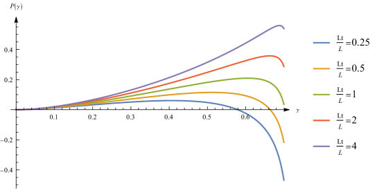
Figure 4: Plot of the expression defined in eq. (3.108) as a function of $\gamma.$ Various colors correspond to different choices of $\tilde{L}/L$.

The divergence structure obtained in Eq. (3.107) is of the same kind as the one predicted using the volume conjecture [68]. Indeed, we found using the double cutoff regularization:

$$\Delta\mathcal{C}_{V}^{\rm JAdS}=\frac{L}{G}\,\eta(\gamma)\log\left(\frac{l}{\delta}\right)+\,\,{\rm finite\,\,terms}\,,$$ (3.109)

where

$$\eta(\gamma)=2\alpha_{+}\left(\mathbb{K}(m)-\mathbb{E}(m)\right)\,.$$ (3.110)

The plot of the function $\eta(\gamma)$ is shown in Fig. 5. The contribution intrinsic to the defect $\Delta\mathcal{C}_{V}^{\rm JAdS}$ is always positive and diverges when $\gamma\rightarrow 1/\sqrt{2}$.

Figure 5: Plot of $\eta(\gamma)$ as defined in Eq. (3.110), which is the coefficient of the log divergences due to the defect in the volume case.

At small $\gamma$, the coefficient of the volume divergent term [68] scales as $\gamma^{2}$, i.e. $\eta\approx\pi\gamma^{2}/4$. From the eq. (3.108), we checked that the coefficient $\mathcal{O}(\gamma)$ of the small $\gamma$ expansion of $P$ indeed vanishes, i.e.

$$P(\gamma,{\tilde{L}}/{L})=c_{1}\gamma^{2}+c_{2}\gamma^{2}\log\gamma^{2}+\mathcal{O}(\gamma^{3})\,,$$ (3.111)

where

$$c_{1}=\frac{15}{8\pi}-\frac{5\pi}{64}+\frac{3\pi}{32}\log\left|\frac{8}{3\pi}\frac{\tilde{L}}{L}\right|\,,\qquad c_{2}=-\frac{3\pi}{32}\,.$$ (3.112)

The divergent parts of volume and action have then a similar (even if not identical) parametric dependence at small $\gamma$.

4 Subregion complexity in the AdS₃/BCFT₂ model

In this section we compute the subregion complexity in the AdS₃/BCFT₂ model. The CFT is restricted to live on a half plane of the flat spacetime $x\geq 0$, because there is a boundary at $x=0$. In the present work we are interested to determine if the presence of this boundary entails a logarithmically divergent complexity. In principle, we could consider the case of an arbitrary interval $x\in[l_{1},l_{2}]$, which, in general, does not contain the boundary at $x=0$. If the interval does not contain the boundary, we do not expect extra divergences in addition to the ones of pure AdS (this was explicitly checked for the CV case in [64]). Therefore we will consider the subregion complexity of the interval $x\in[0,l/2].$

In section 4.1 we specify the domain of integration, see Fig. 6. We perform the calculation of the action in section 4.2. In order to find the intrinsic contribution coming from the presence of the brane, we will subtract the vacuum solution.

4.1 Null boundaries in the AdS₃/BCFT₂ model

We work with the metric in Poincaré coordinates $X^{\mu}=(t,z,x)$, see eq. (2.9). The bulk dual geometry is delimited by the end-of-the-world brane

$$x=-z\,\cot\alpha\,.$$ (4.1)

The RT surface at $t=0$ is the same as in pure AdS

$$z_{\rm RT}(x)=\sqrt{\left(\frac{l}{2}\right)^{2}-x^{2}}\,.$$ (4.2)

The EW and most of the WDW patch are also the same as the ones in empty AdS space. An extra portion of WDW patch (see [64, 65]) is also needed.

We use the regularization A in Fig. 2 where the WDW patch and the EW start from the true boundary located at $z=0.$ The cutoff is the surface $z=\delta.$ At the end of the computation, we will send $\delta\rightarrow 0.$

WDW patch. Here we consider just the $t>0$ boundary of the WDW, the $t<0$ part can be found by symmetry. The null boundary of the WDW patch in the right region $x\geq 0$ originating from the surface at $t=0$ and $z=0$ is

$$t_{\rm WDW,R}(z,x)=z\,.$$ (4.3)

In the left region $x<0,$ the boundary of the WDW patch is a portion of the cone

$$t_{\rm WDW,L}(z,x)=\sqrt{x^{2}+z^{2}}\,,$$ (4.4)

which intersects the brane defined by eq. (4.1). The null boundary of this portion of WDW patch can be parametrized by the congruence of geodesics

$$X^{\mu}_{\rm WDW,L}=B\,(\lambda,\lambda\cos\theta,-\lambda\sin\theta)\,,$$ (4.5)

where each value of $\theta\in[0,\frac{\pi}{2}-\alpha]$ gives a different null geodesic, $\lambda$ is the (non-affine) geodesic parameter and $B>0$ is an arbitrary constant. The relevant geometric quantities are

$$k^{\mu}_{\rm WDW,L}=B\,(1,\cos\theta,-\sin\theta)\,,\quad\kappa_{\rm WDW,L}=-\frac{2}{\lambda}\,,\quad\sqrt{\gamma_{\rm WDW,L}}=\frac{L}{\cos\theta}\,,\quad\Theta_{\rm WDW,L}=0\,.$$ (4.6)

Entanglement wedge. The boundary of the EW is the same as in pure AdS

$$t_{\rm EW}(z,x)=\frac{l}{2}-\sqrt{x^{2}+z^{2}}\,.$$ (4.7)

The tangent vector of the null affine geodesics is

$$w^{\mu}=C\,\frac{z^{2}}{L^{2}}\left(-1,\frac{z}{\sqrt{x^{2}+z^{2}}},\frac{x}{\sqrt{x^{2}+z^{2}}}\right)\,,$$ (4.8)

where $C>0$ is a constant. The expansion parameter $\Theta$ vanishes as expected [85].

Intersection between surfaces. The following intersection curves play an important role in delimiting the integration regions:

• The intersection curve between the right side of the WDW patch and the EW:

  $$x_{\rm int,R}(z)=\frac{1}{2}\sqrt{l(l-4z)}\,,\qquad t_{\rm int,R}(z)=z\,.$$ (4.9)

• The intersection between the left part of the WDW patch and the EW:

  $$x_{\rm int,L}(z)=-\sqrt{\left(\frac{l}{4}\right)^{2}-z^{2}}\,,\qquad t_{\rm int,L}(z)=\frac{l}{4}\,.$$ (4.10)

The intersection between the curve in eq. (4.10) and the end-of-the-world brane is the point:

$$(t_{1},z_{1},x_{1})=\left(\frac{l}{4},\frac{l}{4}\sin\alpha,-\frac{l}{4}\cos\alpha\right)\,.$$ (4.11)

It is useful to determine the intersection between the RT geodesic in eq. (4.2) and the brane in eq. (4.1), which is the point with coordinates

$$(t_{2},z_{2},x_{2})=\left(0\,,\frac{l}{2}\sin\alpha\,,-\frac{l}{2}\cos\alpha\right)\,.$$ (4.12)

The following inequalities hold

$$z_{1}<z_{2}\,,\qquad\left|x_{1}\right|<\left|x_{2}\right|\,.$$ (4.13)

The intersection between the RT and the cutoff surface is the point with coordinates

$$(t_{3},z_{3},x_{3})=\left(0\,,\delta\,,\frac{1}{2}\sqrt{l^{2}-4\delta^{2}}\right)\,.$$ (4.14)

Note that $x_{3}$ is different from $x_{\rm int,R}$ evaluated at $z=\delta,$ which is instead

$$x_{\rm int,R}(\delta)=\frac{1}{2}\sqrt{l(l-4\delta)}\,,$$ (4.15)

and in particular

$$x_{3}\geq x_{\rm int,R}(\delta)\,.$$ (4.16)

Therefore, when splitting the evaluation of the gravitational action using regularization A in Fig. 2, we need to include the contribution from spacetime regions in this interval. The full geometric setting is depicted in Fig. 6. A projection on the $(x,z)$ plane is shown in figure 7.

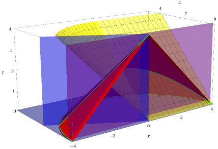
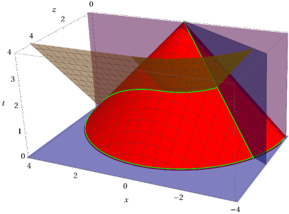
Figure 6: Geometrical sketch of the null boundaries of the WDW patch (light yellow surfaces) and of the entanglement wedge (red), taken from two different perspectives. The blue plane represents the brane and restricts the intergration to the region $x\geq-z\cot\alpha.$ The purple transparent region represents the cutoff surfaces located at $z=\delta.$ There are several curves depicted in green representing the intersections between the WDW patch, the entanglement wedge and the brane. In the figure we take $\alpha=\pi/6.$

4.2 Computation of the action

The evaluation of the subregion action is composed by two parts: the right side of the conformal diagram in Fig. 6, which is the same as in empty AdS space, and the left side where the end-of-the-world brane modifies the geometry to consider. The former contribution for symmetry reasons is half of the subregion action evaluated in AdS₃ spacetime, which was studied in [12, 45, 48]:

$$I_{\rm R}=\frac{L}{8\pi G}\log\left|\frac{\tilde{L}}{L}\right|\,\frac{l}{\delta}+\frac{L}{4\pi G}\log\left|\frac{2\tilde{L}}{L}\right|\log\left(\frac{\delta}{l}\right)-\frac{L}{4\pi G}\log\left|\frac{\tilde{L}}{L}\right|+\frac{L\pi}{32G}\,.$$ (4.17)

Now we proceed with the computation of the left side.

4.2.1 Bulk term

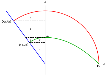
Figure 7: Projection on the $(x,z)$ plane of the integration domain. It corresponds to figure 6 seen from above (where for ”above” we mean large positive $t$). The end-of-the-world brane is shown in blue and the RT surface is drawn in red. The intersection curve in eqs. (4.9) and (4.10) is shown in green. The splitting of integration in eq. (4.18) for the bulk term for $\alpha\geq{\pi}/{6}$ is also shown. The integrals $I^{1}_{\mathcal{B},L},\dots,I^{5}_{\mathcal{B},L}$ correspond to the regions $1,\dots,5$.

Using the decomposition in figure 7, for $\alpha\geq{\pi}/{6}$ we can split the computation of the left side of the bulk term as follows

$$I_{\mathcal{B},L}=2\left(I^{1}_{\mathcal{B},L}+I^{2}_{\mathcal{B},L}+I^{3}_{\mathcal{B},L}+I^{4}_{\mathcal{B},L}+I^{5}_{\mathcal{B},L}\right)\,,$$ (4.18)

where

$$I^{1}_{\mathcal{B},L} = -\frac{L}{4\pi G}\int_{\delta}^{z_{1}}dz\int_{-z\cot\alpha}^{0}dx\int_{0}^{t_{\rm WDW,L}(z,x)}dt\,\frac{1}{z^{3}}\,,$$

$$I^{2}_{\mathcal{B},L} = -\frac{L}{4\pi G}\int_{z_{1}}^{l/4}dz\int_{x_{\rm int,L}(z)}^{0}dx\int_{0}^{t_{\rm WDW,L}(z,x)}dt\,\frac{1}{z^{3}}\,,$$

$$I^{3}_{\mathcal{B},L} = -\frac{L}{4\pi G}\int_{z_{1}}^{l/4}dz\int_{-z\cot\alpha}^{x_{\rm int,L}(z)}dx\int_{0}^{t_{\rm EW}(z,x)}dt\,\frac{1}{z^{3}}\,,$$ (4.19)

$$I^{4}_{\mathcal{B},L} = -\frac{L}{4\pi G}\int_{l/4}^{z_{2}}dz\int_{-z\cot\alpha}^{0}dx\int_{0}^{t_{\rm EW}(z,x)}dt\,\frac{1}{z^{3}}\,,$$

$$I^{5}_{\mathcal{B},L} = -\frac{L}{4\pi G}\int_{z_{2}}^{l/2}dz\int_{\sqrt{(l/2)^{2}-z^{2}}}^{0}dx\int_{0}^{t_{\rm EW}(z,x)}dt\,\frac{1}{z^{3}}\,.$$

The integrals $I^{1}_{\mathcal{B},L},\dots,I^{5}_{\mathcal{B},L}$ are performed respectively in the domains $1,\dots,5$ shown in figure 7. In eq. (4.18), we put a factor of 2 to account for the part of the geometry at negative times. In the evaluation of the gravitational action, we need to consider the spacetime region given by the intersection between the EW and the WDW patch, which are delimited by their respective null boundaries. Using the symmetry along the time direction, the recipe is to integrate along $t$ from 0 up to the smaller value between $t_{\rm WDW,L}(z,x)$ and $t_{\rm EW}(z,x).$ In the following, we will refer to the application of this prescription by stating that either the WDW patch sits below the EW, or viceversa. Here by ”below” we mean being closer to the plane $t=0$, see figure 6. The intersection curves depicted in green in Fig. 6 and 7 delimit the region where the time coordinate of the EW patch becomes bigger than the WDW patch, or similar transitions in the splitting of the geometrical decomposition.

The first two terms in eq. (4.18) refer to the region where the WDW patch is below the EW, and therefore the integration along $t$ goes from 0 to the function $t_{\rm WDW,L}(z,x).$ The terms $I^{3}_{\mathcal{B},L},I^{4}_{\mathcal{B},L},I^{5}_{\mathcal{B},L}$ correspond instead to the spacetime region where the EW sits below the WDW patch.

Strictly speaking, the decomposition in eq. (4.19) only applies when $\alpha\geq{\pi}/{6}.$ For $\alpha<{\pi}/{6},$ the splitting is slightly different and the integrals to evaluate get modified. However there is nothing singular at the special value $\alpha={\pi}/{6}:$ rather, the distinction arises from the splitting of the integration domains. We verified by direct computation that the result for $\alpha<{\pi}/{6}$ is given by the same analytical formula.

We find that the relevant divergences all come from the first contribution

$$I^{1}_{\mathcal{B},L} =\frac{L}{8\pi G}\left[\frac{\cot\alpha}{\sin\alpha}-\log\left(\tan\left(\frac{\alpha}{2}\right)\right)\right]\left[\log\left(\frac{\delta}{l}\right)-\log\left(\frac{\sin\alpha}{4}\right)\right]\,,$$ (4.20)

while the other terms contribute only to finite parts. Summing all these contributions, we get

$$I_{\mathcal{B},L}= \frac{L}{4\pi G}\left[\frac{\cot\alpha}{\sin\alpha}-\log\left(\tan\left(\frac{\alpha}{2}\right)\right)\right]\left[\log\left(\frac{\delta}{l}\right)-\log\left(\frac{\sin\alpha}{4}\right)\right]$$ (4.21)

$$+\frac{L}{96\pi G}\left[\pi^{2}-36\,\frac{\cot\alpha}{\sin\alpha}-6\log^{2}2-12\log^{2}\left(\sin\alpha\right)+6\log\left(4-4\cos\alpha\right)\log\left(1-\cos\alpha\right)\right.$$

$$\left.+12\log\left(\tan\left(\frac{\alpha}{2}\right)\right)-24\log\left(2\sin\alpha\right)\log\left(\tan\left(\frac{\alpha}{2}\right)\right)+24\,\frac{\cot\alpha}{\sin\alpha}\,\log 2-12\mathrm{Li}_{2}\left(\sin^{2}\left(\frac{\alpha}{2}\right)\right)\right]\,.$$

The divergent part is all contained into the logarithm in the first line; everything else amounts to a finite part.

4.2.2 GHY term

The contribution to the GHY term in the left region is evaluated exactly in the same way as in [64], since the presence of the entanglement wedge does not modify this part. Indeed, for small enough $\delta,$ the cutoff only intersects the WDW patch; therefore we obtain (including a symmetry factor of 2):

$$I_{\rm GHY,L}=\frac{L}{2\pi G}\int_{-\delta\cot\alpha}^{0}dx\int_{0}^{t_{\rm WDW,L}(\delta,x)}\frac{dt}{\delta^{2}}=\frac{L}{4\pi G}\left[\frac{\cot\alpha}{\sin\alpha}-\log\left(\tan\left(\frac{\alpha}{2}\right)\right)\right]\,.$$ (4.22)

Unlike the computation in [64], here there is no IR cutoff because the finite length of the subregion on the boundary works as a regulator.

4.2.3 Brane term

The brane term is a codimension-one contribution coming from the surface $\mathcal{Q}$ parametrized by $x=-z\cot\alpha.$ For the brane, the outward-directed normal vector, induced metric and extrinsic curvature are

$$n^{\mu}=-\frac{z}{L}\left(0,\cos\alpha,\sin\alpha\right)\,,\quad ds^{2}=\frac{L^{2}}{z^{2}}\left(-dt^{2}+\frac{dz^{2}}{\sin^{2}\alpha}\right)\,,\quad\sqrt{-h}=\frac{L^{2}}{z^{2}}\frac{1}{\sin\alpha}\,,\quad K=\frac{2\cos\alpha}{L}\,,$$ (4.23)

while the tension is given in eq. (2.11). The brane term can be splitted into a contribution coming from the intersection with the WDW patch, and the other one coming from the intersection with the EW. After including a symmetry factor of 2 to account for negative times, we compute these terms as follows:

$$I_{\mathcal{Q}}=2\left(I^{1}_{\mathcal{Q}}+I^{2}_{\mathcal{Q}}\right)\,,$$ (4.24)

where

$$I^{1}_{\mathcal{Q}} = \frac{1}{8\pi G}\int_{\delta}^{z_{\rm int,L}(\alpha)}dz\int_{0}^{t_{\rm WDW,L}(z,x=-z\cot\alpha)}dt\,\frac{L}{z^{2}}\cot\alpha=\frac{L}{8\pi G}\frac{\cot\alpha}{\sin\alpha}\log\left(\frac{l}{4\delta}\sin\alpha\right)\,,$$

$$I^{2}_{\mathcal{Q}} = \frac{1}{8\pi G}\int_{z_{\rm int,L}(\alpha)}^{z_{\rm max,L}(\alpha)}dz\int_{0}^{t_{\rm EW}(z,x=-z\cot\alpha)}dt\,\frac{L}{z^{2}}\cot\alpha=\frac{L}{8\pi G}\frac{\cot\alpha}{\sin\alpha}\left(1-\log 2\right)\,.$$ (4.25)

Summing the two contributions, we find

$$I_{\mathcal{Q}}=\frac{L}{4\pi G}\frac{\cot\alpha}{\sin\alpha}\left[\log\left(\frac{l}{\delta}\right)+1+\log\left(\frac{\sin\alpha}{8}\right)\right]\,.$$ (4.26)

4.2.4 Joint terms

There are several joint terms to include:

• Joint between the cutoff surface $z=\delta$ and the brane $\mathcal{Q}.$
  This joint involves two timelike surfaces. The induced metric is determined by imposing $z=\delta$ and $x=-z\cot\alpha,$ so that

  $$ds^{2}=-\frac{L^{2}}{z^{2}}dt^{2}\,,\qquad\sqrt{-h}=\frac{L}{\delta}\,.$$ (4.27)

  In addition, the argument of the integrand corresponds to the boost parameter relating the cutoff and the brane, and reads

  $$\eta=\left|\mathrm{arccos}\,\left(\mathbf{n}\cdot\mathbf{n}_{\delta}\right)\right|=\alpha\,,$$ (4.28)

  where $\mathbf{n}$ is defined in eq. (4.23) and $\mathbf{n}_{\delta}$ is the normal one-form to the cutoff surface. This joint is fully contained in the region where the WDW patch sits below the EW, and therefore the integration along the coordinate $t$ runs along the range $[0,t_{\rm WDW,L}(z=\delta,x=-\delta\cot\alpha)].$ Explicitly, this is given by

  $$I_{\mathcal{J},\rm L}^{\mathcal{Q},\delta}=\frac{1}{4\pi G}\int_{0}^{\frac{\delta}{\sin\alpha}}dt\,\frac{\alpha L}{\delta}=\frac{L}{4\pi G}\frac{\alpha}{\sin\alpha}\,.$$ (4.29)

  We included here a symmetry factor of 2 to include also the region at negative times. This expression is the same appearing in [64].

• Joint between the WDW patch and the cutoff surface $z=\delta.$
  The WDW patch at $z=\delta$ is given by $t_{\rm WDW,L}(\delta,x)=\sqrt{x^{2}+\delta^{2}}.$ Therefore the induced metric reads

  $$ds^{2}=\frac{L^{2}}{z^{2}}\left[-\left(\frac{dt_{\rm WDW,L}}{dx}\right)^{2}+1\right]dx^{2}\,,\qquad\sqrt{\gamma}=\frac{L}{\cos\theta}\,,$$ (4.30)

  where we are using for convenience polar coordinates such that $\theta=-\mathrm{\arctan}\,(x/z).$ The scalar product between the normal one-forms is

  $$\mathfrak{a}=\log\left|\mathbf{n}_{\delta}\cdot\mathbf{k}_{\rm WDW,L}\right|=\log\left|\frac{BL\cos\theta}{\delta}\right|\,.$$ (4.31)

  This allows to evaluate

  $$I_{\mathcal{J},\rm L}^{\rm WDW,\delta} =-\frac{L}{4\pi G}\int_{0}^{\frac{\pi}{2}-\alpha}\frac{d\theta}{\cos\theta}\log\left|\frac{BL\cos\theta}{\delta}\right|=$$ (4.32)

  $$=\frac{L}{4\pi G}\log\left(\tan\left(\frac{\alpha}{2}\right)\right)\log\left(\frac{BL}{\delta}\right)$$

  $$-\frac{L}{96\pi G}\left[\pi^{2}+12\log\left(\tan\left(\frac{\alpha}{2}\right)\right)\log\left(\frac{1}{4}\tan\left(\frac{\alpha}{2}\right)\right)+12\mathrm{Li}_{2}\left(-\cot^{2}\left(\frac{\alpha}{2}\right)\right)\right]\,.$$

  where we assigned $\eta_{\eta}=-1$ sign due to the fact that the joint is a past boundary for the WDW patch, and the spacetime region of interest is also in the past with respect to the null boundary of the WDW patch. In addition, we put a symmetry factor of 2. There would be in principle a joint term from the intersection between the cutoff surface at $z=\delta$ and the EW, but since the brane delimits the spacetime region of integration, this intersection is cut away.

• Joint at the RT surface.
  The computation works in the same way as for empty AdS spacetime, the only difference being that the lower endpoint of integration along $x$ is determined by putting $x=-z\cot\alpha$ in the equation defining the RT surface. We get

  $$I_{\mathcal{J},\rm L}^{\rm RT} = -\frac{L}{8\pi G}\int_{-\frac{l}{2}\cos\alpha}^{0}dx\,\frac{2l}{l^{2}-4x^{2}}\log\left|\frac{C^{2}}{4L^{2}}\left(l^{2}-4x^{2}\right)\right|$$ (4.33)

  $$= \frac{L}{4\pi G}\log\left(\tan\left(\frac{\alpha}{2}\right)\right)\log\left(\frac{Cl}{L}\right)$$

  $$-\frac{L}{96\pi G}\left[\pi^{2}+12\log^{2}\left(\tan\left(\frac{\alpha}{2}\right)\right)+12\mathrm{Li}_{2}\left(-\cot^{2}\left(\frac{\alpha}{2}\right)\right)\right]\,.$$

  We notice that this joint amounts only to a finite part.

• Joint at the intersection curve between WDW patch and EW.
  The induced metric is

  $$ds^{2}=\frac{L^{2}}{z^{2}}\left[\left(\frac{dz_{\rm int,L}}{dx}\right)^{2}+1\right]dz^{2}=\frac{L^{2}}{z_{\rm int,L}^{2}}\frac{l^{2}}{l^{2}-16x^{2}}dz^{2}\,,\qquad\sqrt{\gamma}=\frac{4l}{l^{2}-16x^{2}}\,,$$ (4.34)

  and the integrand contains the factor

  $$\mathfrak{a}=\log\left|\mathbf{k}_{\rm WDW,L}\cdot\mathbf{w}\right|=\log\left|BC\right|\,.$$ (4.35)

  In this computation, we used the fact that the intersection curve is located at constant $t=l/4.$ Therefore we obtain (putting a symmetry factor of 2)

  $$I_{\mathcal{J},\rm R}^{\rm int}=\frac{L}{4\pi G}\int_{-\frac{l}{4}\cos\alpha}^{0}dx\,\frac{4l}{l^{2}-16x^{2}}\log\left(BC\right)=-\frac{L}{4\pi G}\log\left(BC\right)\log\left(\tan\left(\frac{\alpha}{2}\right)\right)\,.$$ (4.36)

• Joint between orthogonal surfaces
  There are three joints between orthogonal surfaces. One of them is between the two parts of the WDW patch at $x=0$ and involves two parallel null surfaces. The other two involve the joints between the brane and the WDW patch and the EW, respectively. All of them have a potentially divergent integrand, which involve the logarithm of the scalar product of two orthogonal vectors. However, the integrand is multiplied by the vanishing determinant of the induced metric. Although formally undetermined, these terms can be shown to vanish by an opportune limiting procedure [64].

Summing all the joint contributions from the left side of the geometry, we obtain

$$I_{\mathcal{J},\rm L} =-\frac{L}{4\pi G}\log\left(\tan\left(\frac{\alpha}{2}\right)\right)\log\left(\frac{\delta}{l}\right)$$ (4.37)

$$+\frac{L}{48\pi G}\left[12\,\frac{\alpha}{\sin\alpha}-12\log\left(\tan\left(\frac{\alpha}{2}\right)\right)\log\left(\frac{1}{2}\tan\left(\frac{\alpha}{2}\right)\right)-12\mathrm{Li}_{2}\left(-\cot^{2}\left(\frac{\alpha}{2}\right)\right)-\pi^{2}\right]\,.$$

The only divergence is logarithmic and comes from the joint between the WDW patch and the cutoff surface; all the other terms contribute to finite parts. Remarkably, all the dependence on the ambiguity in parametrizing the null vectors cancel, and we obtain a logarithmic divergence in $\delta/l$ plus a finite part which depends only on $\alpha.$

4.2.5 Null boundary term and counterterm

The computation of the codimension-one terms on the WDW patch works in the same way as explained in [65, 64], except that the range of the $\lambda$ coordinate is delimited by the intersection between the WDW patch and the EW. In particular, the biggest value of $z$ reached along the null boundary of the WDW patch is $z=l/4.$ We find

$$I_{\rm\mathcal{N}}^{\rm WDW,L}=-\frac{1}{4\pi G}\int_{0}^{\frac{\pi}{2}-\alpha}d\theta\int_{\frac{\delta}{B\cos\theta}}^{\frac{l}{4B\cos\theta}}d\lambda\,\frac{L}{\cos\theta}\left(-\frac{2}{\lambda}\right)=\frac{L}{2\pi G}\log\left(\tan\left(\frac{\alpha}{2}\right)\right)\log\left(\frac{4\delta}{l}\right)\,.$$ (4.38)

Since the expansion parameter of the congruence of geodesics vanishes both on the left side of the WDW patch and on the boundary of the EW, the counterterm action is zero, $I_{\rm ct}=0$.

One should also consider the analogous terms evaluated on the EW; however they both vanish because the parametrization (4.8) is affine and the expansion parameter vanishes.

4.2.6 Subtraction of the vacuum solution and final result

Summing all the contributions, one observes that the divergences arising from the left side cancel, giving just a finite contribution. There is also a contribution to the total action from the right side, (4.17), which is independent of $\alpha$.

As in [65], we can isolate the contribution of the boundary by subtracting the complexity of the $\alpha=\frac{\pi}{2}$ case, which correspond to a vanishing brane tension, see eq. (2.11). We find that the boundary contribution to the subregion complexity is finite, and independent from $l$ i.e.

$$\Delta\mathcal{C}_{A}^{\rm BCFT}=\frac{L}{96\pi^{2}G} \left\{12\frac{\cot\alpha}{\sin\alpha}-\pi^{2}-6\log^{2}2-12\log^{2}\left(\sin\alpha\right)+24\,\frac{\alpha}{\sin\alpha}-12\log\left(\tan\left(\frac{\alpha}{2}\right)\right)\right.$$ (4.39)

$$\left.+6\log\left(4-4\cos\alpha\right)\log\left(1-\cos\alpha\right)+24\log\left(\tan\left(\frac{\alpha}{2}\right)\right)\log 4\right.$$

$$\left.-24\log^{2}\left(\tan\left(\frac{\alpha}{2}\right)\right)-12\mathrm{Li}_{2}\left(\sin^{2}\left(\frac{\alpha}{2}\right)\right)-24\mathrm{Li}_{2}\left(-\cot^{2}\left(\frac{\alpha}{2}\right)\right)\right\}\,.$$

The result is plotted in Fig. 8, showing a divergent result when $\alpha\rightarrow 0$ and its vanishing value when $\alpha=\frac{\pi}{2}.$

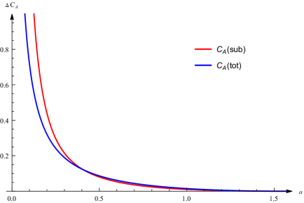
Figure 8: Plot of the contribution of the defect to the subregion complexity in eq. (4.39) as a function of $\alpha$ (red) and comparison with the result for the total space studied in [65] (blue). Here we set $L/G=1$.

As the contribution of the defect $\Delta\mathcal{C}_{A}^{\rm BCFT}$ to the subregion complexity is independent of the subregion size $l$, we may expect that it should reproduce the calculation of the total complexity of formation in [64, 65]. This is not the case, because the choice of the infrared cutoff is different: while in [64, 65] the action is regulated by an IR cutoff at constant $z$, we instead use as an IR cutoff the RT surface. The two choices agree just for the UV divergent part of the action: in fact, this divergence is independent of the infrared regulator because it is localised nearby the location of the defect.

5 Conclusions

In this work we computed the CA conjecture for a subregion given by an interval of length $l$ on the boundary for both the Janus AdS₃ geometry and the AdS₃/BCFT₂ model. As discussed below Table 1, the action conjecture does not provide a universal structure of UV divergences, but the results depend on the particular defect or boundary characterizing the geometry. It was recently proposed that ambiguities in the field theory realization of complexity models could be related to similar ambiguities in the holographic proposal [25]. It would be interesting to investigate if the distinct behaviours of the interface models considered in this paper can be related to such ambiguities.

In [74] we studied the volume conjecture for the non-supersymmetric Janus AdS₅ geometry. We computed the volume using the single and the double cutoff regularizations, and we found that only the coefficient of the log-divergences was independent of the regularization. It would be interesting to check this also for action complexity.

We believe that further insights on the universality properties of the holographic complexity conjecture could arise from an investigation of the subregion action in the moving mirror model, which was studied using the CV conjecture [86]. The moving mirror setting is also a useful tool to investigate the evaporation of black holes. The recent developments coming from the island conjectures [87, 88, 89] have been related to subregion complexity in [90]. It would be interesting to test these conjectures in the models with defects or boundaries considered here.

Appendix A Jacobi elliptic functions and elliptic integrals

We follow the conventions of [91] to define the incomplete elliptic integrals

$$\mathds{F}\left(\left.\varphi\right|m\right) =\int_{0}^{\varphi}\frac{d\theta}{\sqrt{1-m\sin^{2}\theta}}\;,\noindent$$ (A.1)

$$\mathds{E}\left(\left.\varphi\right|m\right) =\int_{0}^{\varphi}d\theta\sqrt{1-m\sin^{2}\theta}\;,\noindent$$ (A.2)

$$\Pi\left(n;\varphi\left|m\right.\right) =\int_{0}^{\varphi}\frac{d\theta}{\left(1-n\sin^{2}\theta\right)\sqrt{1-m\sin^{2}\theta}}.$$ (A.3)

of the first, second and third kind, respectively. The complete elliptic integrals are defined as

$$\mathds{F}\left(\left.\frac{\pi}{2}\right|m\right)=\mathds{K}(m)\;,\quad\mathds{E}\left(\left.\frac{\pi}{2}\right|m\right)=\mathds{E}(m)\;,\quad\Pi\left(n;\frac{\pi}{2}\Big{|}m\right)=\Pi\left(\left.n\right|m\right)\;.$$ (A.4)

The Jacobi amplitude $\varphi=\text{am}(x|m)$ is the inverse of $\mathds{F}\left(\left.x\right|m\right)$

$$x=\mathds{F}\left(\left.\varphi\right|m\right)\;.$$ (A.5)

The Jacobi elliptic functions are defined as

$$\text{sn}\left(\left.\!x\right|m\right)=\sin\varphi,\quad\text{cn}\left(\left.\!x\right|m\right)=\cos\varphi\quad\text{and}\quad\text{dn}\left(\left.\!x\right|m\right)=\sqrt{1-m\sin^{2}\varphi},$$ (A.6)

such that $\text{sn}\left(\left.\!\mathds{K}(m)\right|m\right)=1$ and $\text{cn}\left(\left.\!\mathds{K}(m)\right|m\right)=0$. They satisfy the identities

$$\text{sn}\left(\left.\!x\right|m\right)^{2}+\text{cn}\left(\left.\!x\right|m\right)^{2}=1\;,$$ (A.7)

$$\text{dn}\left(\left.\!x\right|m\right)^{2}+m\,\text{sn}\left(\left.\!x\right|m\right)^{2}=1\;.$$ (A.8)

We conclude with the derivation of the finite form of the change of variables presented in eq. (3.40). Infinitesimally, we apply the transformation in eq. (2.6). Taking eq. (2.4) into account, a direct integration leads to

$$y =\int_{0}^{\mu}ds\,\sqrt{f(s)}$$ (A.9)

$$=\int_{0}^{\mu}ds\,\frac{\alpha_{+}}{\mathrm{sn}\left(\alpha_{+}(s+\mu_{0})|m\right)}$$

$$=\int_{0}^{\alpha_{+}\mu}d\sigma\,\frac{1}{\mathrm{sn}\left(\sigma+\mathds{K}(m)|m\right)}$$

$$=\int_{0}^{\alpha_{+}\mu}d\sigma\,\frac{\mathrm{dn}\left(\sigma|m\right)}{\mathrm{cn}\left(\sigma|m\right)}$$

$$=\frac{1}{2}\mathrm{log}\left(\frac{1+\mathrm{sn}\left(\alpha_{+}\mu|m\right)}{1-\mathrm{sn}\left(\alpha_{+}\mu|m\right)}\right)$$

$$=\mathrm{arctanh}\left[\mathrm{sn}\left(\alpha_{+}\mu|m\right)\right]\,.$$

In the first equation we replaced eq. (2.4), in the second we used the definition of $\mu_{0}$ in eq. (2.5); then the (half)-periodicity property $\mathrm{sn}\left(\sigma+\mathds{K}(m)|m\right)=\mathrm{cn}\left(\sigma|m\right)/\mathrm{dn}\left(\sigma|m\right)$ was taken into account. The resulting (indefinite) integral is known and can be found for example in eq. $(5.135.5)$ of [92]. Inverting the hyperbolic function leads to the form reported in eq. (3.40).

Appendix B Details of the series expansion of Janus AdS action

We report in this Appendix the details of the series-expansion of the terms composing the gravitational action evaluated in section 3.3, following the steps outlined in section 3.3.6.

Using the definition of $\mu_{0}$ in eq. (2.5) and the property $f(\mu^{*}(\varepsilon))=\varepsilon^{-2},$ we obtain (see eq. $(2.12)$ in [67])

$$\mu_{0}-\mu^{*}(\varepsilon)=\frac{1}{\alpha_{+}}\mathds{F}\left(\left.\mathrm{arcsin}\left(\alpha_{+}\varepsilon\right)\right|m\right)=\varepsilon+\mathcal{O}(\varepsilon^{3})\,.$$ (B.1)

This identity is the building block to determine the expansion of the action around $\varepsilon=0,$ and it is sufficient to perform the expansion of the terms of case 1 in Section 3.3.6.

In order to perform the procedure described for the terms of case 2 in Section 3.3.6, the following Laurent-expansions around $\mu=\mu_{0}$ are needed:

$$f(\mu)^{3/2}\,\sin\left(\mu_{0}-\mu\right)=\frac{1}{\left(\mu_{0}-\mu\right)^{2}}+\frac{1}{3}+\mathcal{O}(\mu_{0}-\mu)\,,$$ (B.2)

$$f(\mu)^{3/2}\,\left[\sin\left(\mu_{0}-\mu\right)+1\right]\,\log\left[\sin\left(\mu_{0}-\mu\right)+1\right]=\frac{1}{\left(\mu_{0}-\mu\right)^{2}}+\frac{1}{2\left(\mu_{0}-\mu\right)}+\frac{1}{6}+\mathcal{O}\left(\mu_{0}-\mu\right)\,,$$ (B.3)

$$\sqrt{f(\mu)}\log\left[\sqrt{f(\mu)}\left(\sin\left(\mu_{0}-\mu\right)+1\right)\right]=-\frac{1}{\mu_{0}-\mu}\log\left(\mu_{0}-\mu\right)+1+\mathcal{O}\left[\left(\mu_{0}-\mu\right)\log\left(\mu_{0}-\mu\right)\right]\,.$$ (B.4)

In the following subsection we perform the procedure term by term.

B.1 Expansion of the action term by term

Using the identities and the definitions listed above, we determine the expansions of the terms entering the gravitational action:

• Bulk term. Consider the second term in eq. (3.45), which is analytic in all the integration domain, except for a neighbourhood of $\mu=\mu_{0}.$ Its Laurent-expansion around $\mu=\mu_{0}$ is given in eq. (B.2). The only term contributing to a divergence is the first one, therefore we regularize the integral by adding and subtracting such term, which evaluates to

  $$\int_{0}^{\mu^{*}(\varepsilon)}\frac{d\mu}{\left(\mu_{0}-\mu\right)^{2}}=\frac{1}{\mu_{0}-\mu^{*}(\varepsilon)}-\frac{1}{\mu_{0}}=\frac{1}{\varepsilon}-\frac{1}{\mu_{0}}+\mathcal{O}(\varepsilon)\,$$ (B.5)

  where we used the definition of $\mu_{0}$ in eq. (2.5) and the property $f(\mu^{*}(\varepsilon))=\varepsilon^{-2}$ to obtain the expansion around $\varepsilon=0.$ Now we move to the first part of the integral (3.45). The series expansion of the integrand around $\mu=\mu_{0},$ which is the only point where singularities arise, reads

  $$f(\mu)^{3/2}\,\left[\sin\left(\mu_{0}-\mu\right)+1\right]\,\log\left[\sin\left(\mu_{0}-\mu\right)+1\right]=\frac{1}{\left(\mu_{0}-\mu\right)^{2}}+\frac{1}{2\left(\mu_{0}-\mu\right)}+\frac{1}{6}+\mathcal{O}\left(\mu_{0}-\mu\right)\,.$$ (B.6)

  In this case there are two divergent terms: the first one corresponds precisely to Eq. (B.5), while the second one is computed as follows:

  $$\int_{0}^{\mu^{*}(\varepsilon)}\frac{d\mu}{2\left(\mu_{0}-\mu\right)}=\frac{1}{2}\log\left(\frac{\mu_{0}}{\mu_{0}-\mu^{*}(\varepsilon)}\right)=-\frac{1}{2}\log\left(\frac{\varepsilon}{\mu_{0}}\right)+\mathcal{O}(\varepsilon^{2})\,.$$ (B.7)

  We can now combine all the previous results to find

  $$I_{\mathcal{B}}(\gamma)=\frac{L}{\pi G}\left\{\log\left(\frac{2\delta}{l}\right)\left(\frac{1}{\varepsilon}-\frac{1}{\mu_{0}}\right)-\frac{1}{2}\log\left(\frac{\varepsilon}{\mu_{0}}\right)+\mathcal{I}_{\mathcal{B}}^{(0)}(\gamma)+\left[\log\left(\frac{2\delta}{l}\right)-1\right]\mathcal{I}_{\mathcal{B}}^{(1)}(\gamma)\right\}+\mathcal{O}(\varepsilon)\,,$$ (B.8)

  where $\mathcal{I}_{\mathcal{B}}^{(0)}$ and $\mathcal{I}_{\mathcal{B}}^{(1)}$ are given in (B.20) and (B.21).

• GHY term. The GHY term arising from the cutoff surface located at $z=\delta$ and evaluated in eq. (3.51) is already a finite expression, which we denote as the numerical function (B.22). The GHY contribution coming from the surfaces at $\mu=\pm\mu^{*}(\varepsilon)$ are expanded by means of the identity (B.1). The sum of both terms is given by

  $$I_{\rm GHY}(\gamma)=-\frac{L}{\pi G}\left[\frac{1}{\epsilon}\log\left(\frac{2\delta}{l}\right)+\frac{1}{2}-\frac{1}{2}\,\mathcal{I}_{\rm GHY}(\gamma)\right]+\mathcal{O}(\varepsilon)\,,$$ (B.9)

  where $\mathcal{I}_{\rm GHY}(\gamma)$ is given in eq. (B.22).

• Null boundary term. We consider the expression (3.62) and perform an integration by parts of the second term (which we report here for convenience) to get

  $$\frac{L}{\pi G}\int_{0}^{\mu^{*}(\varepsilon)}d\mu\,\frac{f^{\prime}(\mu)}{2\sqrt{f(\mu)}}\cos\left(\mu_{0}-\mu\right)\left(\log\left(\frac{l}{2\delta}\right)-\log\left(1+\sin\left(\mu_{0}-\mu\right)\right)\right)=$$ (B.10)

  $$=\frac{L}{\pi G}\left[\sqrt{f(\mu)}\cos\left(\mu_{0}-\mu\right)\left(\log\left(\frac{l}{2\delta}\right)-\log\left(1+\sin\left(\mu_{0}-\mu\right)\right)\right)\right]_{0}^{\mu^{*}(\varepsilon)}$$

  $$-\frac{L}{\pi G}\int_{0}^{\mu^{*}(\varepsilon)}d\mu\,\sqrt{f(\mu)}\left\{1+\sin\left(\mu_{0}-\mu\right)\left(\log\left(\frac{l}{2\delta}\right)-\log\left(1+\sin\left(\mu_{0}-\mu\right)\right)-1\right)\right\}\,.$$

  The series expansion of the part without any further integration is simplified by the properties $f(0)=\alpha_{+}^{2}$ and $f(\mu^{*}(\varepsilon))=\varepsilon^{-2}.$ Instead the last line combines with the first term in eq. (3.62) to a simpler expression:

  $$\frac{L}{\pi G}\int_{0}^{\mu^{*}(\varepsilon)}d\mu\,\sqrt{f(\mu)}\left[\sin\left(\mu_{0}-\mu\right)-1\right]=\frac{L}{\pi G}\,\mathcal{I}_{\rm GHY}(\gamma)-\frac{L}{\pi G}\int_{0}^{\mu^{*}(\varepsilon)}d\mu\,\sqrt{f(\mu)}\,.$$ (B.11)

  The last contribution is evaluated using the change of variables $\sqrt{f(\mu)}d\mu=dy.$ Collecting all the results, we get

  $$I_{\mathcal{N}}(\gamma)=\frac{L}{\pi G} \left\{\frac{1}{\varepsilon}\log\left(\frac{l}{2\delta}\right)-\alpha_{+}\cos\mu_{0}\log\left(\frac{l}{2\delta}\right)+\alpha_{+}\cos\mu_{0}\log\left(1+\sin\mu_{0}\right)\right.$$ (B.12)

  $$\left.+\log\left((1-2\gamma^{2})^{1/4}\,\frac{\varepsilon}{2}\right)+\mathcal{I}_{\rm GHY}(\gamma)-1\right\}+\mathcal{O}(\varepsilon)\,.$$

• Joint terms. Most of the joint terms can be evaluated immediately using the identity (B.1) and the numerical functions defined in Appendix B.2. We also need this explicit integral, giving a divergent part:

  $$\int_{0}^{\mu^{*}(\varepsilon)}\frac{d\mu}{\mu_{0}-\mu}\log\left(\mu_{0}-\mu\right)=-\frac{1}{2}\left(\log^{2}\varepsilon-\log^{2}\mu_{0}\right)+\mathcal{O}(\varepsilon)\,.$$ (B.13)

  The result for the total joint action is

  $$I_{\mathcal{J}}(\gamma)=I^{\delta,\rm WDW}_{\mathcal{J}}(\gamma)+I^{\varepsilon,\rm WDW}_{\mathcal{J}}(\gamma)+I_{\mathcal{J}}^{\rm RT}(\gamma)+I_{\mathcal{J}}^{\rm int}(\gamma)+I^{\mu}_{\mathcal{J}}(\gamma)\,,$$ (B.14)

  where

  $$I^{\delta,\rm WDW}_{\mathcal{J}}(\gamma)=-\frac{L}{2\pi G}\left[\log\left(\frac{\alpha L}{\delta}\right)\mathcal{I}_{\rm GHY}(\gamma)+\mathcal{I}_{\mathcal{J}}^{(0)}(\gamma)\right]\,,$$ (B.15)

  $$I^{\varepsilon,\rm WDW}_{\mathcal{J}}(\gamma)=\frac{L}{4\pi G}\left\{\frac{1}{\varepsilon}\left[2\log\left(\frac{\alpha L}{\varepsilon}\right)\log\left(\frac{2\delta}{l}\right)-\log^{2}\delta+\log^{2}\left(\frac{2}{l}\right)\right]+2\log\left(\frac{2\alpha L}{l\varepsilon}\right)\right\}+\mathcal{O}(\varepsilon)\,,$$ (B.16)

  $$I_{\mathcal{J}}^{\rm RT}(\gamma)+I_{\mathcal{J}}^{\rm int}(\gamma)=\frac{L}{2\pi G}\left\{\frac{1}{2}\log^{2}\varepsilon-\log\left(\frac{\alpha L}{l}\right)\log\left(\left(1-2\gamma^{2}\right)^{1/4}\frac{\varepsilon}{2}\right)-\frac{1}{2}\log^{2}\mu_{0}+\,\mathcal{I}_{\mathcal{J}}^{(1)}(\gamma)\right\}+\mathcal{O}(\varepsilon)\,,$$ (B.17)

  $$I^{\mu}_{\mathcal{J}}(\gamma) =-\frac{L\alpha_{+}\,\cos\mu_{0}}{4\pi G}\left\{2\log|\alpha L\alpha_{+}\cos\mu_{0}|\log\left(\frac{2\delta}{l}\right)\right.$$ (B.18)

  $$\left.+2\log\left|\alpha L\alpha_{+}\cos\mu_{0}\right|\log\left(1+\sin\mu_{0}\right)-\log^{2}\delta+\log^{2}\left(\frac{2(1+\sin\mu_{0})}{l}\right)\right\}+\mathcal{O}(\varepsilon)\,,$$

  where the functions $\mathcal{I}_{\mathcal{J}}^{(0)}(\gamma)$ and $\mathcal{I}_{\mathcal{J}}^{(1)}(\gamma)$ are respectively defined in eqs. (B.23) and (B.24). It is relevant to observe that the ambiguity in the normalization of the null normals to the boundary of the EW, parametrized by $\beta,$ cancels once we combine the joints at the RT surface and at the intersection between WDW patch and EW.

• Counterterm. The treatment of the counterterm is similar to the null boundary term; since the expression is rather cumbersome, we directly report the result:

  $$I_{\rm ct}^{\rm WDW}(\gamma) =\frac{L}{4\pi G}\left\{2\log\left(\frac{2\alpha\tilde{L}}{l}\right)\log\left((1-2\gamma^{2})^{1/4}\,\frac{\varepsilon}{2}\right)+2\log\left(\frac{2\alpha\tilde{L}}{l}\right)\mathcal{I}_{\rm GHY}(\gamma)+\log^{2}\mu_{0}-\log^{2}\varepsilon\right.$$ (B.19)

  $$\left.+\mathcal{I}_{\rm ct}^{(0)}(\gamma)+2\log\left(\frac{2\delta}{l}\right)\left(\frac{1}{\varepsilon}-\frac{1}{\mu_{0}}\right)+\log\left(\frac{2\delta}{l}\right)\mathcal{I}_{\rm ct}^{(1)}(\gamma)+2\log\left(\frac{\mu_{0}}{\varepsilon}\right)+\mathcal{I}_{\rm ct}^{(2)}(\gamma)\right.$$

  $$\left.-\frac{1}{\varepsilon}\left[2\log\left(\frac{\alpha\tilde{L}}{\varepsilon}\right)\log\left(\frac{2\delta}{l}\right)-\log^{2}\delta+\log^{2}\left(\frac{2}{l}\right)\right]-2\log\left(\frac{2\alpha\tilde{L}}{l\varepsilon}\right)\right.$$

  $$\left.+\alpha_{+}\cos\mu_{0}\left[2\log\left(\alpha\tilde{L}\sin\mu_{0}\right)\log\left(\frac{2\delta}{l}\right)+2\log\left(\alpha\tilde{L}\sin\mu_{0}\right)\log\left(1+\sin\mu_{0}\right)\right]\right.$$

  $$\left.+\alpha_{+}\cos\mu_{0}\left[\log^{2}\left(\frac{2\left(1+\sin\mu_{0}\right)}{l}\right)-\log^{2}\delta\right]\right\}+\mathcal{O}(\varepsilon)\,,$$

  where the numerical functions $\mathcal{I}_{\rm ct}^{(0)},\mathcal{I}_{\rm ct}^{(1)}$ ar defined in eqs. (B.25) and (B.26).

B.2 Collection of numerical functions

We collect here all the numerical functions obtained from the regularization procedure applied in Appendix B.1:

$$\mathcal{I}_{\mathcal{B}}^{(0)}(\gamma)\equiv\int_{0}^{\mu_{0}}d\mu\,\left\{f(\mu)^{3/2}\left[\left(\sin\left(\mu_{0}-\mu\right)+1\right)\log\left(\sin\left(\mu_{0}-\mu\right)+1\right)\right]-\frac{1}{\left(\mu_{0}-\mu\right)^{2}}-\frac{1}{2\left(\mu_{0}-\mu\right)}\right\}\,,$$ (B.20)

$$\mathcal{I}_{\mathcal{B}}^{(1)}(\gamma)\equiv\int_{0}^{\mu_{0}}d\mu\,\left[f(\mu)^{3/2}\sin\left(\mu_{0}-\mu\right)-\frac{1}{\left(\mu_{0}-\mu\right)^{2}}\right]\,,$$ (B.21)

$$\mathcal{I}_{\rm GHY}(\gamma)\equiv\int_{0}^{\mu_{0}}d\mu\sqrt{f(\mu)}\sin(\mu_{0}-\mu)\,,$$ (B.22)

$$\mathcal{I}_{\mathcal{J}}^{(0)}(\gamma)\equiv\int_{0}^{\mu_{0}}d\mu\sqrt{f(\mu)}\sin(\mu_{0}-\mu)\log\left(\sqrt{f(\mu)}\sin(\mu_{0}-\mu)\right)\;,$$ (B.23)

$$\mathcal{I}_{\mathcal{J}}^{(1)}(\gamma)\equiv\int_{0}^{\mu_{0}}d\mu\,\left\{\sqrt{f(\mu)}\,\log\left[\sqrt{f(\mu)}\left(1+\sin\left(\mu_{0}-\mu\right)\right)\right]+\frac{1}{\mu_{0}-\mu}\log\left(\mu_{0}-\mu\right)\right\}\,,$$ (B.24)

$$\mathcal{I}_{\rm ct}^{(0)}(\gamma)\equiv\int_{0}^{\mu_{0}}d\mu \left\{-2\sqrt{f(\mu)}\left(1-\sin\left(\mu_{0}-\mu\right)\right)\log\left[\left(\sin\left(\mu_{0}-\mu\right)+\frac{f^{\prime}(\mu)}{2f(\mu)}\cos\left(\mu_{0}-\mu\right)\right)\right.\right.$$ (B.25)

$$\left.\left.\times\left(1+\sin\left(\mu_{0}-\mu\right)\right)\right]-\frac{2}{\mu_{0}-\mu}\log\left(\mu_{0}-\mu\right)\right\}\,,$$

$$\mathcal{I}_{\rm ct}^{(1)}(\gamma)\equiv\int_{0}^{\mu_{0}}d\mu\,\left[\frac{-2\sqrt{f(\mu)}K(\mu)}{2f(\mu)\sin\left(\mu_{0}-\mu\right)+f^{\prime}(\mu)\cos\left(\mu_{0}-\mu\right)}-\frac{2}{\left(\mu_{0}-\mu\right)^{2}}\right]\,,$$ (B.26)

$$K(\mu)\equiv \,2\cos^{2}\left(\mu_{0}-\mu\right)f(\mu)+\cos^{2}\left(\mu_{0}-\mu\right)\frac{f^{\prime}(\mu)^{2}}{f(\mu)}$$ (B.27)

$$-\sin\left(\mu_{0}-\mu\right)\cos\left(\mu_{0}-\mu\right)f^{\prime}(\mu)-\cos^{2}\left(\mu_{0}-\mu\right)f^{\prime\prime}(\mu)\,.$$

Appendix C Counterterms on timelike boundaries

In this Appendix we consider the inclusion in the action of the counterterm introduced in [75, 76], which for $d=2$ is

$$I_{\rm ct}^{\rm cutoff}=-\frac{1}{8\pi G}\int dx\,dt\,\sqrt{-h}\,\frac{1}{L}\,,$$ (C.1)

where $h$ is the metric determinant of the induced metric on the boundary. This term was introduced in [75, 76] for the regularization prescription A in Fig. 2, in order to reproduce the divergences of regularization B.

C.1 Janus AdS₃ geometry

In the Janus AdS₃ background there are two timelike regulator surfaces:

• The first timelike cutoff surface corresponds to $z=\delta,$ and its contribution reads

  $$I^{\delta}_{\rm ct}=-\frac{L}{2\pi G}\int_{0}^{\mu^{*}(\delta)}d\mu\int_{\delta}^{t_{\rm WDW}(\delta,\mu)}dt\,\frac{f(\mu)}{\delta}=-\frac{L}{2\pi G}\int_{0}^{\mu^{*}(\varepsilon)}d\mu\,f(\mu)\,\sin\left(\mu_{0}-\mu\right)\,,$$ (C.2)

  where we put a symmetry factor of 4. The integrand gives rise to divergences due to the singularity in $\mu=\mu_{0}.$ Therefore we Laurent-expand the function around this point

  $$f(\mu)\sin\left(\mu_{0}-\mu\right)=\frac{1}{\mu_{0}-\mu}+\mathcal{O}\left(\mu_{0}-\mu\right)\,.$$ (C.3)

  Adding and subtracting this divergence allows to find

  $$I_{\rm ct}^{\delta}=-\frac{L}{2\pi G}\left[\log\left(\frac{\mu_{0}}{\varepsilon}\right)+\mathcal{I}_{\rm ct}^{\delta}(\gamma)\right]+\mathcal{O}(\varepsilon)\,,$$ (C.4)

  where we define the numerical function

  $$\mathcal{I}_{\rm ct}^{\delta}(\gamma)\equiv\int_{0}^{\mu_{0}}d\mu\,\left(f(\mu)\sin\left(\mu_{0}-\mu\right)-\frac{1}{\mu_{0}-\mu}\right)\,,$$ (C.5)

  such that $\mathcal{I}_{\rm ct}^{\delta}(0)=\log\left(\frac{4}{\pi}\right).$ After subtracting the vacuum AdS solution, we find

  $$\Delta I_{\rm ct}^{\delta}=-\frac{L}{2\pi G}\left[\log\left(\frac{\mu_{0}}{2}\right)+\mathcal{I}_{\rm ct}^{\delta}(\gamma)\right]\,.$$ (C.6)

• The second timelike cutoff surface corresponds to $\mu=\mu^{*}(\varepsilon)$ and to its partner located at $\mu=-\mu^{*}(\varepsilon),$ which contributes to the same result by symmetry reasonings. We find

  $$I^{\varepsilon}_{\rm ct} =-\frac{L}{2\pi G\varepsilon^{2}}\left\{\int_{\delta}^{z_{\rm int}(\mu^{*}(\varepsilon))}\frac{dz}{z}\,\sin\left(\mu_{0}-\mu^{*}(\varepsilon)\right)+\int_{z_{\rm int}(\mu^{*}(\varepsilon))}^{z_{\rm RT}}\frac{dz}{z^{2}}\,\left(\frac{l}{2}-z\right)\right\}=$$ (C.7)

  $$=\frac{L}{2\pi G}\left[\frac{1}{\varepsilon}\log\left(\frac{2\delta}{l}\right)-\frac{1}{2}\right]+\mathcal{O}(\varepsilon)\,.$$

  After subtracting the vacuum AdS solution, this simply vanishes, $\Delta I_{\rm ct}^{\varepsilon}=0$.

Therefore, the total contribution coming from timelike counterterms in the Janus AdS background amounts to a finite part given in eq. (C.6).

C.2 AdS₃/BCFT₂ model

The AdS/BCFT model contains a cutoff surface located at $z=\delta.$ Since the extrinsic curvature on the cutoff surface at $z=\delta$ is $K=2/L,$ the timelike counterterm (C.1) is proportional to the corresponding GHY contribution:

$$I_{\rm ct}^{\delta}=-\frac{1}{2}I^{\delta}_{\rm GHY}=-\frac{L}{8\pi G}\left[\frac{\cot\alpha}{\sin\alpha}-\log\left(\tan\left(\frac{\alpha}{2}\right)\right)\right]\,.$$ (C.8)

The vacuum solution corresponds to $\alpha=\frac{\pi}{2},$ but for this value the action vanishes. Therefore we directly obtain that the same result holds after the subtraction, $\Delta I_{\rm ct}^{\delta}=I_{\rm ct}^{\delta}$.

References

- [1] S. Ryu and T. Takayanagi, “Holographic derivation of entanglement entropy from AdS/CFT,” Phys. Rev. Lett. 96 (2006) 181602, hep-th/0603001.
- [2] J. M. Maldacena, “The Large N limit of superconformal field theories and supergravity,” Adv. Theor. Math. Phys. 2 (1998) 231–252, hep-th/9711200.
- [3] L. Susskind, “Computational Complexity and Black Hole Horizons,” Fortsch. Phys. 64 (2016) 24–43, 1403.5695. [Addendum: Fortsch.Phys. 64, 44–48 (2016)].
- [4] L. Susskind, “Entanglement is not enough,” Fortsch. Phys. 64 (2016) 49–71, 1411.0690.
- [5] M. A. Nielsen, “A geometric approach to quantum circuit lower bounds,” Quantum Information and Computation 6 (05, 2006) quant-ph/0502070.
- [6] M. A. N. Mark R. Dowling, “The geometry of quantum computation,” Quantum Information and Computation 8 (01, 2010) 861, quant-ph/0701004.
- [7] S. Aaronson, “The Complexity of Quantum States and Transformations: From Quantum Money to Black Holes,” 7, 2016. 1607.05256.
- [8] D. Stanford and L. Susskind, “Complexity and Shock Wave Geometries,” Phys. Rev. D 90 (2014), no. 12, 126007, 1406.2678.
- [9] A. R. Brown, D. A. Roberts, L. Susskind, B. Swingle, and Y. Zhao, “Holographic Complexity Equals Bulk Action?,” Phys. Rev. Lett. 116 (2016), no. 19, 191301, 1509.07876.
- [10] A. R. Brown, D. A. Roberts, L. Susskind, B. Swingle, and Y. Zhao, “Complexity, action, and black holes,” Phys. Rev. D 93 (2016), no. 8, 086006, 1512.04993.
- [11] L. Lehner, R. C. Myers, E. Poisson, and R. D. Sorkin, “Gravitational action with null boundaries,” Phys. Rev. D 94 (2016), no. 8, 084046, 1609.00207.
- [12] D. Carmi, R. C. Myers, and P. Rath, “Comments on Holographic Complexity,” JHEP 03 (2017) 118, 1612.00433.
- [13] S. Chapman, H. Marrochio, and R. C. Myers, “Complexity of Formation in Holography,” JHEP 01 (2017) 062, 1610.08063.
- [14] J. Couch, W. Fischler, and P. H. Nguyen, “Noether charge, black hole volume, and complexity,” JHEP 03 (2017) 119, 1610.02038.
- [15] R.-G. Cai, S.-M. Ruan, S.-J. Wang, R.-Q. Yang, and R.-H. Peng, “Action growth for AdS black holes,” JHEP 09 (2016) 161, 1606.08307.
- [16] A. Reynolds and S. F. Ross, “Divergences in Holographic Complexity,” Class. Quant. Grav. 34 (2017), no. 10, 105004, 1612.05439.
- [17] D. Carmi, S. Chapman, H. Marrochio, R. C. Myers, and S. Sugishita, “On the Time Dependence of Holographic Complexity,” JHEP 11 (2017) 188, 1709.10184.
- [18] R. Auzzi, S. Baiguera, and G. Nardelli, “Volume and complexity for warped AdS black holes,” JHEP 06 (2018) 063, 1804.07521.
- [19] R. Auzzi, S. Baiguera, M. Grassi, G. Nardelli, and N. Zenoni, “Complexity and action for warped AdS black holes,” JHEP 09 (2018) 013, 1806.06216.
- [20] M. Alishahiha, A. Faraji Astaneh, M. R. Mohammadi Mozaffar, and A. Mollabashi, “Complexity Growth with Lifshitz Scaling and Hyperscaling Violation,” JHEP 07 (2018) 042, 1802.06740.
- [21] S. Bolognesi, E. Rabinovici, and S. R. Roy, “On Some Universal Features of the Holographic Quantum Complexity of Bulk Singularities,” JHEP 06 (2018) 016, 1802.02045.
- [22] A. Bernamonti, F. Galli, J. Hernandez, R. C. Myers, S.-M. Ruan, and J. Simón, “First Law of Holographic Complexity,” Phys. Rev. Lett. 123 (2019), no. 8, 081601, 1903.04511.
- [23] S. S. Hashemi, G. Jafari, and A. Naseh, “First law of holographic complexity,” Phys. Rev. D 102 (2020), no. 10, 106008, 1912.10436.
- [24] A. Bernamonti, F. Bigazzi, D. Billo, L. Faggi, and F. Galli, “Holographic and QFT complexity with angular momentum,” JHEP 11 (2021) 037, 2108.09281.
- [25] A. Belin, R. C. Myers, S.-M. Ruan, G. Sárosi, and A. J. Speranza, “Complexity Equals Anything?,” 2111.02429.
- [26] A. R. Brown and L. Susskind, “Complexity geometry of a single qubit,” Phys. Rev. D 100 (2019), no. 4, 046020, 1903.12621.
- [27] V. Balasubramanian, M. Decross, A. Kar, and O. Parrikar, “Quantum Complexity of Time Evolution with Chaotic Hamiltonians,” JHEP 01 (2020) 134, 1905.05765.
- [28] R. Auzzi, S. Baiguera, G. B. De Luca, A. Legramandi, G. Nardelli, and N. Zenoni, “Geometry of quantum complexity,” Phys. Rev. D 103 (2021), no. 10, 106021, 2011.07601.
- [29] V. Balasubramanian, M. DeCross, A. Kar, Y. C. Li, and O. Parrikar, “Complexity growth in integrable and chaotic models,” JHEP 07 (2021) 011, 2101.02209.
- [30] A. R. Brown, M. H. Freedman, H. W. Lin, and L. Susskind, “Effective Geometry, Complexity, and Universality,” 2111.12700.
- [31] R. Jefferson and R. C. Myers, “Circuit complexity in quantum field theory,” JHEP 10 (2017) 107, 1707.08570.
- [32] S. Chapman, M. P. Heller, H. Marrochio, and F. Pastawski, “Toward a Definition of Complexity for Quantum Field Theory States,” Phys. Rev. Lett. 120 (2018), no. 12, 121602, 1707.08582.
- [33] R. Khan, C. Krishnan, and S. Sharma, “Circuit Complexity in Fermionic Field Theory,” Phys. Rev. D 98 (2018), no. 12, 126001, 1801.07620.
- [34] M. Doroudiani, A. Naseh, and R. Pirmoradian, “Complexity for Charged Thermofield Double States,” JHEP 01 (2020) 120, 1910.08806.
- [35] P. Caputa, N. Kundu, M. Miyaji, T. Takayanagi, and K. Watanabe, “Anti-de Sitter Space from Optimization of Path Integrals in Conformal Field Theories,” Phys. Rev. Lett. 119 (2017), no. 7, 071602, 1703.00456.
- [36] P. Caputa and J. M. Magan, “Quantum Computation as Gravity,” Phys. Rev. Lett. 122 (2019), no. 23, 231302, 1807.04422.
- [37] J. Erdmenger, M. Gerbershagen, and A.-L. Weigel, “Complexity measures from geometric actions on Virasoro and Kac-Moody orbits,” JHEP 11 (2020) 003, 2004.03619.
- [38] M. Flory and M. P. Heller, “Geometry of Complexity in Conformal Field Theory,” Phys. Rev. Res. 2 (2020), no. 4, 043438, 2005.02415.
- [39] N. Chagnet, S. Chapman, J. de Boer, and C. Zukowski, “Complexity for Conformal Field Theories in General Dimensions,” 2103.06920.
- [40] J. Boruch, P. Caputa, D. Ge, and T. Takayanagi, “Holographic path-integral optimization,” JHEP 07 (2021) 016, 2104.00010.
- [41] J. Couch, Y. Fan, and S. Shashi, “Circuit Complexity in Topological Quantum Field Theory,” 2108.13427.
- [42] L. Susskind, “Three Lectures on Complexity and Black Holes,” SpringerBriefs in Physics. Springer, 10, 2018. 1810.11563.
- [43] S. Chapman and G. Policastro, “Quantum Computational Complexity – From Quantum Information to Black Holes and Back,” 2110.14672.
- [44] C. A. Agón, M. Headrick, and B. Swingle, “Subsystem Complexity and Holography,” JHEP 02 (2019) 145, 1804.01561.
- [45] E. Caceres, S. Chapman, J. D. Couch, J. P. Hernandez, R. C. Myers, and S.-M. Ruan, “Complexity of Mixed States in QFT and Holography,” JHEP 03 (2020) 012, 1909.10557.
- [46] M. Alishahiha, “Holographic Complexity,” Phys. Rev. D 92 (2015), no. 12, 126009, 1509.06614.
- [47] R. Abt, J. Erdmenger, H. Hinrichsen, C. M. Melby-Thompson, R. Meyer, C. Northe, and I. A. Reyes, “Topological Complexity in AdS3/CFT2,” Fortsch. Phys. 66 (2018), no. 6, 1800034, 1710.01327.
- [48] R. Auzzi, S. Baiguera, A. Legramandi, G. Nardelli, P. Roy, and N. Zenoni, “On subregion action complexity in AdS3 and in the BTZ black hole,” JHEP 01 (2020) 066, 1910.00526.
- [49] B. Chen, W.-M. Li, R.-Q. Yang, C.-Y. Zhang, and S.-J. Zhang, “Holographic subregion complexity under a thermal quench,” JHEP 07 (2018) 034, 1803.06680.
- [50] M. Alishahiha, K. Babaei Velni, and M. R. Mohammadi Mozaffar, “Black hole subregion action and complexity,” Phys. Rev. D 99 (2019), no. 12, 126016, 1809.06031.
- [51] R. Auzzi, S. Baiguera, A. Mitra, G. Nardelli, and N. Zenoni, “Subsystem complexity in warped AdS,” JHEP 09 (2019) 114, 1906.09345.
- [52] R. Auzzi, G. Nardelli, F. I. Schaposnik Massolo, G. Tallarita, and N. Zenoni, “On volume subregion complexity in Vaidya spacetime,” JHEP 11 (2019) 098, 1908.10832.
- [53] G. Di Giulio and E. Tonni, “Subsystem complexity after a global quantum quench,” JHEP 05 (2021) 022, 2102.02764.
- [54] G. Di Giulio and E. Tonni, “Subsystem complexity after a local quantum quench,” JHEP 08 (2021) 135, 2106.08282.
- [55] M. Banados, M. Henneaux, C. Teitelboim, and J. Zanelli, “Geometry of the (2+1) black hole,” Phys. Rev. D 48 (1993) 1506–1525, gr-qc/9302012. [Erratum: Phys.Rev.D 88, 069902 (2013)].
- [56] L. Susskind and Y. Zhao, “Switchbacks and the Bridge to Nowhere,” 1408.2823.
- [57] M. Flory, “A complexity/fidelity susceptibility -theorem for AdS3/BCFT2,” JHEP 06 (2017) 131, 1702.06386.
- [58] L. Randall and R. Sundrum, “An Alternative to compactification,” Phys. Rev. Lett. 83 (1999) 4690–4693, hep-th/9906064.
- [59] S. Chapman, D. Ge, and G. Policastro, “Holographic Complexity for Defects Distinguishes Action from Volume,” JHEP 05 (2019) 049, 1811.12549.
- [60] C. Bachas, J. de Boer, R. Dijkgraaf, and H. Ooguri, “Permeable conformal walls and holography,” JHEP 06 (2002) 027, hep-th/0111210.
- [61] T. Takayanagi, “Holographic Dual of BCFT,” Phys. Rev. Lett. 107 (2011) 101602, 1105.5165.
- [62] M. Fujita, T. Takayanagi, and E. Tonni, “Aspects of AdS/BCFT,” JHEP 11 (2011) 043, 1108.5152.
- [63] M. Nozaki, T. Takayanagi, and T. Ugajin, “Central Charges for BCFTs and Holography,” JHEP 06 (2012) 066, 1205.1573.
- [64] P. Braccia, A. L. Cotrone, and E. Tonni, “Complexity in the presence of a boundary,” JHEP 02 (2020) 051, 1910.03489.
- [65] Y. Sato and K. Watanabe, “Does Boundary Distinguish Complexities?,” JHEP 11 (2019) 132, 1908.11094.
- [66] D. Bak, M. Gutperle, and S. Hirano, “A Dilatonic deformation of AdS(5) and its field theory dual,” JHEP 05 (2003) 072, hep-th/0304129.
- [67] D. Bak, M. Gutperle, and S. Hirano, “Three dimensional Janus and time-dependent black holes,” JHEP 02 (2007) 068, hep-th/0701108.
- [68] R. Auzzi, S. Baiguera, S. Bonansea, G. Nardelli, and K. Toccacelo, “Volume complexity for Janus geometries,” JHEP 08 (2021) 045, 2105.08729.
- [69] J. Estes, K. Jensen, A. O’Bannon, E. Tsatis, and T. Wrase, “On Holographic Defect Entropy,” JHEP 05 (2014) 084, 1403.6475.
- [70] D. Bak, A. Gustavsson, and S.-J. Rey, “Conformal Janus on Euclidean Sphere,” JHEP 12 (2016) 025, 1605.00857.
- [71] M. Gutperle and A. Trivella, “Note on entanglement entropy and regularization in holographic interface theories,” Phys. Rev. D 95 (2017), no. 6, 066009, 1611.07595.
- [72] D. Z. Freedman, C. Nunez, M. Schnabl, and K. Skenderis, “Fake supergravity and domain wall stability,” Phys. Rev. D 69 (2004) 104027, hep-th/0312055.
- [73] I. Papadimitriou and K. Skenderis, “Correlation functions in holographic RG flows,” JHEP 10 (2004) 075, hep-th/0407071.
- [74] S. Baiguera, S. Bonansea, and K. Toccacelo, “Volume complexity for the nonsupersymmetric Janus AdS5 geometry,” Phys. Rev. D 104 (2021), no. 8, 086030, 2105.12743.
- [75] A. Akhavan and F. Omidi, “On the Role of Counterterms in Holographic Complexity,” JHEP 11 (2019) 054, 1906.09561.
- [76] F. Omidi, “Regularizations of Action-Complexity for a Pure BTZ Black Hole Microstate,” JHEP 07 (2020) 020, 2004.11628.
- [77] V. Balasubramanian and P. Kraus, “A Stress tensor for Anti-de Sitter gravity,” Commun. Math. Phys. 208 (1999) 413–428, hep-th/9902121.
- [78] S. de Haro, S. N. Solodukhin, and K. Skenderis, “Holographic reconstruction of space-time and renormalization in the AdS / CFT correspondence,” Commun. Math. Phys. 217 (2001) 595–622, hep-th/0002230.
- [79] M. Bianchi, D. Z. Freedman, and K. Skenderis, “Holographic renormalization,” Nucl. Phys. B 631 (2002) 159–194, hep-th/0112119.
- [80] K. Skenderis, “Lecture notes on holographic renormalization,” Class. Quant. Grav. 19 (2002) 5849–5876, hep-th/0209067.
- [81] E. Poisson, A Relativist’s Toolkit: The Mathematics of Black-Hole Mechanics. Cambridge University Press, 12, 2009.
- [82] M. Blau, Lecture Notes on General Relativity.
- [83] R. M. Wald, General Relativity. Chicago Univ. Pr., Chicago, USA, 1984.
- [84] T. Azeyanagi, A. Karch, T. Takayanagi, and E. G. Thompson, “Holographic calculation of boundary entropy,” JHEP 03 (2008) 054, 0712.1850.
- [85] M. Headrick, V. E. Hubeny, A. Lawrence, and M. Rangamani, “Causality \& holographic entanglement entropy,” JHEP 12 (2014) 162, 1408.6300.
- [86] Y. Sato, “Complexity in a moving mirror model,” 2108.04637.
- [87] A. Almheiri, R. Mahajan, J. Maldacena, and Y. Zhao, “The Page curve of Hawking radiation from semiclassical geometry,” JHEP 03 (2020) 149, 1908.10996.
- [88] A. Almheiri, N. Engelhardt, D. Marolf, and H. Maxfield, “The entropy of bulk quantum fields and the entanglement wedge of an evaporating black hole,” JHEP 12 (2019) 063, 1905.08762.
- [89] G. Penington, “Entanglement Wedge Reconstruction and the Information Paradox,” JHEP 09 (2020) 002, 1905.08255.
- [90] J. Hernandez, R. C. Myers, and S.-M. Ruan, “Quantum extremal islands made easy. Part III. Complexity on the brane,” JHEP 02 (2021) 173, 2010.16398.
- [91] M. Abramowitz and I. Stegun, Handbook of Mathematical Functions. fifth edition, Dover (1964), New York.
- [92] I. S. Gradshteyn and I. M. Ryzhik, Table of integrals, series, and products. Academic press, 2014.