Quasinormal modes of Proca fields in a Schwarzschild-AdS spacetime

Abstract

We present new results concerning the Proca massive vector field in a Schwarzschild-anti-de Sitter (Schwarzschild-AdS) black hole geometry. We provide a first principles analysis of Proca vector fields in this geometry using both the vector spherical harmonic (VSH) decomposition and separation method and the Frolov-Krtouš-Kubizňák-Santos (FKKS) method that separates the relevant equations in spinning geometries. The analysis in the VSH method shows, on one hand, that it is arduous to separate the scalar-type from the vector-type polarizations of the electric sector of the Proca field, and on the other hand, it displays clearly the electric and the magnetic mode sectors. The analysis in the FKKS method is performed by taking the nonrotating limit of the Kerr-AdS spacetime, and shows that the Ansatz decouples the polarizations in the electric mode sector even in the nonrotating limit. On the other hand, it captures only two of the three possible polarizations; indeed, the magnetic mode sector, which is of vector-type, is missing. The reason for the absence of the remaining polarization is related to the degeneracy of the principal tensor in static spherical symmetric spacetimes. The degrees of freedom and quasinormal modes in both separation methods of the Proca field are found. The frequencies of the quasinormal modes are also carefully computed. For the electric mode sector in the VSH method the frequencies are found through an extension, which substitutes number coefficients by matrix coefficients, of the Horowitz-Hubeny numerical procedure, whereas for the magnetic mode sector in the VSH method and the electric sector of the FKKS method it is shown that a direct use of the procedure can be made. The values of the quasinormal mode frequencies obtained for each method are compared and shown to be in good agreement with each other. This further supports the analytical approaches presented here for the behavior of the Proca field in a Schwarzschild-AdS black hole background.

I Introduction

Vector fields are known to describe the electroweak and the strong interactions of the standard model of particle physics. In particular, the mediator of electromagnetic interactions is the photon and it can be identified as an excitation of an Abelian massless vector field. Since the standard model does not explain the existence of dark matter, new kinds of fields have been proposed as candidates. Such fields would have very feeble interactions with ordinary matter, but would interact gravitationally. Thus, bodies with strong gravitational effects serve as devices to probe the existence of such new fields. General relativistic black holes and their dynamical description are thus important to understand the behavior of possible new matter, such as massive vector fields that obey the Proca equations.

The analysis of the Maxwell massless vector field in static spacetimes has been performed using the vector spherical harmonics method, or VSH method for short. In Schwarzschild spacetimes, the Maxwell equations were separated, decoupled, and reduced to a single master equation in Ruffini:1973 . In Schwarzschild-anti-de Sitter (Schwarzschild-AdS) spacetimes, the Maxwell equations and their quasinormal mode content were studied using reflective boundary conditions at infinity with VSH techniques in Cardoso:2001 ; ckl , and using vanishing energy flux boundary conditions at infinity, the quasinormal modes were found in WangHerdeiroSampaio ; ChenChoCornell . The massive Proca field in Schwarzschild-type spacetimes with an interest on its late time behavior was studied in KZM , and a quasinormal mode analysis for Schwarzschild spacetimes was performed in Rosa:2012 . Quasinormal modes in Schwarzschild-AdS spacetimes with a focus on their monopole term were analyzed in Konoplya:2006 .

The separation of massless vector fields, such as the Maxwell field, in the Kerr spacetime used a completely different approach, that of the Newman-Penrose formalism, despite the reduced group of explicit symmetries Teukolsky:1972 . This already hinted at the existence of another kind of symmetry. Massive vector fields were considered not only under a small rotation approximation with the equations yielding a ladder of coupled multipoles Pani:2012vp , but also without approximations using a fully numerical approach Witek:2012tr ; Cardoso:2018tly . In a different development, and following previous work Frolov:2008jr ; Houri:2008ng ; Frolov:2017whj ; Frolov:2017 ; Lunin:2017 that takes into account the presence of the principal tensor in the Kerr-NUT-AdS and Kerr-NUT-dS spacetimes, i.e., spacetimes describing a rotating black hole in four and higher dimensions and that include the NUT parameters and a cosmological constant, Frolov, Krtouš, Kubizňák, and Santos Frolov:2018 , or FKKS for short, were able to extend the perturbation analysis to the case of a Proca massive vector field in spinning geometries. It was further shown that with this formalism the Proca equations can be separated. It is still unclear whether the FKKS method covers all the degrees of freedom, including polarizations and quasinormal modes, of the Proca field in the whole Kerr-NUT-AdS and Kerr-NUT-dS family. However, with the help of an analysis for the marginally bound state case Dolan:2018dqv ; Baumann:2019eav , it was found that for the Kerr spacetime the FKKS Ansatz describes all possible modes. The quasinormal modes for the FKKS Ansatz in Kerr were then recalculated and found to yield excellent agreement with previous approaches Percival:2020skc . The investigation of the degrees of freedom covered by the FKKS Ansatz in spinning geometries can be performed either in a small spin approximation or numerically, whereas analytically, this investigation is arduous due to the complexity of the system comprised of partial differential equations and a polynomial equation.

In this paper, we analyze Proca fields in the Schwarzschild-AdS spacetime through both the VSH and the FKKS techniques, i.e., we investigate the degrees of freedom and quasinormal modes through both methods. In the computation of the quasinormal modes, we use reflective boundary conditions at infinity and pure incoming wave boundary conditions at the event horizon. The analysis in the VSH method has the advantage that both the electric and the magnetic sectors appear in a natural way. The analysis in the FKKS method has the advantage that the polarizations in the electric mode sector decouple promptly. To do this we use a useful numerical procedure set up by Horowitz and Hubeny Horowitz:2000 to study perturbations for scalar fields in Schwarzschild-AdS spacetimes and to find their quasinormal mode frequencies, see also cl . An extension of this method which substitutes the number coefficients by matrix coefficients will be performed by us here, see also Delsate:2011qp . For a review of all these treatments and an overview of the FKKS Ansatz see the thesis thesis .

The paper is organized as follows. In Sec. II, we present the general Einstein-Proca field equations and specialize them for a fixed background geometry with a negative cosmological constant. In Sec. III, we separate the Proca equations for a Schwarzschild-AdS spacetime using the VSH method and compute its quasinormal modes. In Sec. IV, we present the FKKS method adapted to the Kerr-AdS spacetime, take the nonrotating limit to the Schwarzschild-AdS spacetime and compute its quasinormal modes. In Sec. V, we compare the quasinormal modes given by the VSH and FKKS methods. In Sec. VI, we conclude. Geometric units $G=c=1$ are used throughout the paper.

II Einstein-Proca field equations with a negative cosmological constant: Fixed background

The action for the minimally coupled Einstein-Proca system is given by

$$S=\int\differential[4]x\sqrt{-g}(\mathcal{L}_{EH}-\mathcal{L}_{A})\,,$$ (1)

where $g$ is the determinant of the metric $g_{ab}$,

$$\mathcal{L}_{EH}=\frac{R-2\Lambda}{16\pi}$$ (2)

is the Einstein-Hilbert Lagrangian density with $R=R_{ab}g^{ab}$, and $R_{ab}$ the Ricci tensor, both built out of the Riemann tensor ${R^{a}}_{bcd}$ made of the metric and its first and second derivatives. $\Lambda$ is the cosmological constant, with which we can define a characteristic length $l=\sqrt{\frac{3}{\absolutevalue{\Lambda}}}$, and

$$\mathcal{L}_{A}=\frac{F_{ab}F^{ab}}{4}+\frac{\mu^{2}}{2}A_{a}A^{a}\,,$$ (3)

is the Proca Lagrangian density with $F_{ab}$, given by $F_{ab}=\nabla_{a}A_{b}-\nabla_{b}A_{a}$ being the Proca field strength, $A_{a}$ being the Proca vector potential, and $\mu$ the field mass. It follows from the Euler-Lagrange equations for the metric field $g_{ab}$ that the Einstein equation must be obeyed, i.e.,

$$G_{ab}+\Lambda g_{ab}=8\pi T_{ab}\,,$$ (4)

where $G_{ab}$ is the Einstein tensor defined as $G_{ab}=R_{ab}-\frac{1}{2}g_{ab}R$, and $T_{ab}$ is the energy-momentum tensor given by

$$T_{ab}=F_{ac}F_{bd}g^{cd}-\frac{1}{4}g_{ab}F_{cd}F^{cd}+\mu^{2}\left(A_{a}A_{b}-\frac{1}{2}g_{ab}A_{c}A^{c}\right)\,.$$ (5)

It follows from the Euler-Lagrange equations for the Proca field $A_{a}$ that the Proca equation must be obeyed, i.e.,

$$\nabla_{b}F^{ab}+\mu^{2}A^{a}=0\,.$$ (6)

The tensor field $F_{ab}$ also obeys the internal equations $\nabla_{[a}F_{bc]}=0$.

The Einstein-Proca system consists of nonlinear coupled partial differential equations, Eqs. (4)-(6). We now want to study the perturbations of the $A_{a}$ field in a fixed background with negative cosmological constant, $\Lambda<0$. In other words, we consider a perturbative expansion of the field equations when the vector field and its derivatives are small. In this case, from Eq. (4) one has the vacuum Einstein equation, namely,

$$G_{ab}-\frac{3}{l^{2}}g_{ab}=0\,.$$ (7)

Now, Eq. (7) obeys the field Bianchi identities, $\nabla_{a}\left(G^{ab}-\frac{3}{l^{2}}g^{ab}\right)=0$. Although to first order the stress-energy tensor $T_{ab}$ is zero, in second order it is not; it must obey the conservation equation

$$\nabla_{a}T^{ab}=0\,,$$ (8)

where $T_{ab}$ is the Proca energy-momentum tensor given in Eq. (5). For the Proca equation given in Eq. (6), one can make use of the commutation relations for covariant derivatives that involve the Riemann tensor to yield $g^{cd}\nabla_{c}\nabla_{d}A^{a}-\mu^{2}A^{a}-R^{a}_{\,\,d}A^{d}=0$, where use of the Bianchi identity for the Proca field was also made. In a background spacetime with a negative cosmological constant, we have from Eq. (7) that $R_{ab}=-\frac{3}{l^{2}}g_{ab}$. So the Proca equation in a fixed negative cosmological constant background becomes

$$g^{cd}\nabla_{c}\nabla_{d}A^{a}-\left(\mu^{2}-\frac{3}{l^{2}}\right)A^{a}=0\,.$$ (9)

The Bianchi identity for the Proca $A^{a}$ field is clearly

$$\nabla_{a}A^{a}=0\,,$$ (10)

i.e., its divergence is zero. Note that for the massless case, $\mu=0$, the Bianchi identity given in Eq. (10) is the Lorenz gauge condition that may or may not be imposed, indeed in this case the field equations are invariant under the gauge transformation $A_{a}\rightarrow A_{a}+\nabla_{a}\chi$, where $\chi$ is a scalar obeying the Klein-Gordon equation, i.e. $\nabla_{a}\nabla^{a}\chi=0$.

Thus, to study the perturbations of the Proca field $A_{a}$ with a fixed spacetime background, and thus a fixed metric, one uses Eq. (9) with the help of Eq. (10). Of interest is the case in which the cosmological constant is negative and the background is a Schwarzschild-AdS black hole. We apply two methods to solve the Proca set of equations given in Eqs. (9) and (10), the VSH and the FKKS methods.

III Proca field perturbations in Schwarzschild-AdS: The VSH method

III.1 Schwarzschild-AdS metric

The spacetime considered here is the Schwarzschild-AdS spacetime, whose line element can be written in spherical $(t,r,\theta,\phi)$ coordinates as

$$ds^{2}=-f(r)dt^{2}+\dfrac{dr^{2}}{f(r)}+r^{2}(d\theta^{2}+\sin^{2}\theta d\phi^{2})\,,$$ (11)

where the function $f(r)$ is

$$f(r)=1-\frac{2M}{r}+\frac{r^{2}}{l^{2}}\,,$$ (12)

and $M$ is the spacetime mass. The Schwarzschild-AdS metric describes a vacuum spherically symmetric spacetime with a negative cosmological constant. It is a static black hole solution with an event horizon located at $r_{+}$ given by the positive root of the equation $f(r)=0$, i.e.,

$$r_{+}^{3}+r_{+}l^{2}-2Ml^{2}=0\,.$$ (13)

III.2 Perturbations in the Proca field, separation of variables, and the VSH method

III.2.1 General case

In the Schwarzschild-AdS spacetime, the Proca equations (9) can be separated using vector spherical harmonics which can be obtained by the sum of a spin $s=1$ with angular momentum $\ell$ as it is well known from any modern quantum mechanics textbook. This vector spherical harmonics method, or VSH method, was first used in Ruffini:1973 to separate the Maxwell equations in static geometries. In the VSH method the following Ansatz is assumed for the field $A_{a}$,

$$A_{a}=\frac{1}{r}\sum_{i=0}^{3}\sum_{lm}c_{i}u_{(i)}(t,r)Z_{a}^{(i)\ell m}(\theta,\phi)\,,$$ (14)

where $c_{0}=1$, $c_{1}=1$, $c_{2}=\frac{1}{\left[\ell(\ell+1)\right]^{\frac{1}{2}}}$, $c_{3}=\frac{1}{\left[\ell(\ell+1)\right]^{\frac{1}{2}}}$, the $u_{(i)}$, with $i=0,1,2,3$, are functions of $t$ and $r$ that should be written as $u_{(i)}(t,r)\equiv u_{(i)}^{\ell m}(t,r)$, but the indices $\ell$ and $m$ have been suppressed to not overcrowd the notation, and the $Z_{a}^{(i)\ell m}$ are given by

$$Z_{a}^{(0)\ell m} =(1,0,0,0)Y^{\ell m}\,,$$ (15)

$$Z_{a}^{(1)\ell m} =(0,\dfrac{1}{f},0,0)Y^{\ell m}\,,$$ (16)

$$Z_{a}^{(2)\ell m} =\frac{r}{\sqrt{\ell(\ell+1)}}(0,0,\partial_{\theta},\partial_{\phi})Y^{\ell m}\,,$$ (17)

$$Z_{a}^{(3)\ell m} =\frac{r}{\sqrt{\ell(\ell+1)}}\Bigg{(}0,0,\frac{\partial_{\phi}}{\sin\theta},-\sin\theta\partial_{\theta}\Bigg{)}Y^{\ell m}\,,$$ (18)

where $Y^{\ell m}$ are the spherical harmonics, with $\ell$ being the principal number and $m$ the azimuthal number.

Indeed, by inserting the Ansatz given in Eq. (14) into the Proca equations (9), one finds after rearrangement the following system of equations for the functions $u_{(i)}$,

$${\hat{\mathcal{D}}}^{2}u_{(0)}+(\partial_{r}f)(\dot{u}_{(1)}-u^{\prime}_{(0)})=0\,,$$ (19)

$${\hat{\mathcal{D}}}^{2}u_{(1)}+\frac{2f}{r^{2}}\Big{(}1-\frac{3M}{r}\Big{)}(u_{(2)}-u_{(1)})=0\,,$$ (20)

$${\hat{\mathcal{D}}}^{2}u_{(2)}+\Bigg{[}\frac{2f\ell(\ell+1)}{r^{2}}u_{(1)}\Bigg{]}=0\,,$$ (21)

$${\hat{\mathcal{D}}}^{2}u_{(3)}=0\,,$$ (22)

where $\dot{u}_{(i)}=\dfrac{\partial{u_{(i)}}}{\partial t}$, $u^{\prime}_{(i)}=\dfrac{\partial{u_{(i)}}}{\partial r_{*}}$ with $r_{*}$ being defined by $\dfrac{dr_{*}}{dr}=\dfrac{1}{f}$, and where ${\hat{\mathcal{D}}}^{2}$ is shorthand for

$${\hat{\mathcal{D}}}^{2}=-\partial_{t}^{2}+\partial_{r_{*}}^{2}-f\Big{[}\frac{\ell(\ell+1)}{r^{2}}+\mu^{2}\Big{]}\,.$$ (23)

It must be noted that $u_{(0)}$, $u_{(1)}$, and $u_{(2)}$ describe the electric modes since, under parity transformations, $Z^{(0)}_{a}$, $Z^{(1)}_{a}$, and $Z^{(2)}_{a}$ gain a factor of $(-1)^{\ell}$, whereas $u_{(3)}$ describes the magnetic modes since, under parity transformations, $Z^{(3)}_{a}$ gains a factor of $(-1)^{\ell+1}$. All this follows the notation given in Rosa:2012 , where the Proca equations for a pure Schwarzschild background have been presented.

Furthermore, inserting the Ansatz in Eq. (14) into the Bianchi identity given in Eq. (10), $\nabla^{a}A_{a}=0$, one obtains

$$\frac{1}{rf}\Bigg{[}u^{\prime}_{(1)}-\dot{u}_{(0)}+\frac{f}{r}(u_{(1)}-u_{(2)})\Bigg{]}=0\,.$$ (24)

Equation  (24) was used to find Eq. (20). Indeed, the Ansatz given in Eq. (14) when put into Eq. (9) leads directly to $\hat{\mathcal{D}}u_{(1)}+(\partial_{r}f)(\dot{u}_{(0)}-u^{\prime}_{(1)})+\frac{2f^{2}}{r^{2}}(u_{(2)}-u_{(1)})=0$, which upon using Eq. (24) yields Eq. (20).

Therefore, the system consisting of Eqs. (19)-(22), taking into account the definition given in Eq. (23), determines the solution. The Bianchi identity, Eq. (24), also helps in the determination of the solution. For example, the static part of $u_{(0)}$ must be obtained from Eq. (19), but the dynamical part of $u_{(0)}$ can be described by the Bianchi identity Eq. (24). Equations (20) and (21), for $u_{(1)}$ and $u_{(2)}$, are coupled together, whereas Eq. (22), for $u_{(3)}$, is decoupled.

We shall assume that the time dependence of the functions $u_{(0)}$, $u_{(1)}$, $u_{(2)}$, and $u_{(3)}$ goes as $e^{-i\omega t}$. In this case, the system given by Eqs. (19)-(22) can be treated as an eigenvalue problem to $\omega$. We classify the eigenvectors of the system according to the three degrees of freedom, i.e., the three polarizations, of the Proca vector $A_{a}$. These three polarizations consist of one scalar-type polarization and two vector-type polarizations. The electric modes of $A_{a}$, characterized by $u_{(0)}$, $u_{(1)}$, and $u_{(2)}$, possess one scalar-type polarization and one vector-type polarization. The scalar-type polarization of $A_{a}$ has a behavior similar to a scalar field, and can be picked up to the higher $\ell$ modes from the $\ell=0$ mode, which has solely scalar-type polarization. Moreover, setting the Proca mass $\mu$ to zero, $\mu=0$, the scalar-type polarization becomes nonphysical, more precisely, at the massless limit it can be removed by the gauge freedom. The vector-type polarization of $A_{a}$ of the electric modes are then picked up by exclusion, i.e., they are the ones that are not scalar-type. Since the system in the electric mode sector is coupled, it is not trivial to obtain the scalar-type and the vector-type polarization of $A_{a}$ in terms of the functions $u_{(1)}$ and $u_{(2)}$. The magnetic modes of $A_{a}$, characterized by $u_{(3)}$, possess the remaining vector-type polarization.

As an addendum, we note that it is possible to decouple the pair of equations for $u_{(1)}$ and $u_{(2)}$ which are also present in the pure Schwarzschild case, see Rosa:2012 . Equation (21) can be used to find $u_{(1)}$ as a function of $u_{(2)}$, i.e., $u_{(1)}=-\frac{r^{2}\hat{\mathcal{D}}^{2}u_{(2)}}{2f\ell(\ell+1)}$. Substituting this expression in Eq. (20), a decoupled equation for $u_{(2)}$ can be found, $\mathcal{H}\left(ru_{(2)}\right)=0$, where $\mathcal{H}=\hat{\mathcal{D}}^{2}\Big{[}\frac{1}{f}\hat{\mathcal{D}}_{1}^{\,2}\Big{]}-2f(\partial_{r}f)\mu^{2}$ and ${\hat{\mathcal{D}}_{1}}^{\,2}=-\partial_{t}^{2}+\partial_{r_{*}}^{2}-f\Big{[}\frac{\ell(\ell+1)}{r^{2}}+\mu^{2}+\frac{\partial_{r}f}{r}\Big{]}$. Thus, one can decouple the pair of equations in this way by paying the price of increasing the order of the partial differential equations. This happens since $u_{(2)}$ must contain the scalar-type and the vector-type polarizations. In the massless limit, $\mu=0$, the operator $\mathcal{H}$ factorizes, becoming the product between the operators $\hat{\mathcal{D}}^{2}$ and $f^{-1}\hat{\mathcal{D}}_{1}^{\,2}$. One must notice that in this limit, the scalar-type polarization can be removed by the gauge freedom, meaning $u_{(2)}$ will contain both a spurious degree of freedom and the physical vector-type polarization associated with the electric modes. It can be shown that the scalar $\Psi=f^{-1}\mathcal{D}_{1}^{\,2}(ru_{(2)})$ is related to the field strength tensor $F_{ab}$, thus in the massless case it describes appropriately the vector-type polarization related to the electric modes without the spurious degree of freedom. Moreover, the equation $\mathcal{H}(ru_{(2)})=0$ indicates that $\Psi$ will satisfy the same equation as $u_{(3)}$, which means the two vector-type polarizations of the massless vector field become degenerate. For the massive case, the factorization of $\mathcal{H}$ does not appear to be possible, which makes the analytical decoupling difficult.

III.2.2 Monopole case

The monopole case $\ell=0$ for the massive vector field simplifies the system considerably. Only the functions $u_{(0)}$ and $u_{(1)}$ survive, the functions $u_{(2)}$ and $u_{(3)}$ vanish since $Y^{00}$ is a constant. The equation for the function $u_{(0)}$ can be obtained from Eq. (19) together with Eq. (23), to give

$$-\ddot{u}_{(0)}+u_{(0)}^{\prime\prime}+(\partial_{r}f)(\dot{u}_{(1)}-u_{(0)}^{\prime})-f\mu^{2}u_{(0)}=0\,.$$ (25)

The equation for $u_{(1)}$ can be obtained from Eq. (20) together with Eq. (23), i.e.,

$$u^{\prime\prime}_{(1)}-\ddot{u}_{(1)}-f\Big{[}\mu^{2}+\frac{2}{r^{2}}\Big{(}1-\frac{3M}{r}\Big{)}\Big{]}u_{(1)}=0\,.$$ (26)

The Bianchi identity given in Eq. (24) is now

$${\dot{u}}_{(0)}=u^{\prime}_{(1)}+\frac{f}{r}u_{(1)}\,.$$ (27)

Note that for the $\ell=0$ case the function $u_{(0)}$ could be written as $u_{(0)}=u_{(0)\text{s}}(r)+u_{(0)\text{t}}(t,r)$, where $u_{(0)\text{s}}(r)$ is the static part of $u_{(0)}$ and can be obtained directly from Eq. (25), and $u_{(0)\text{t}}(t,r)$ is the dynamic part of $u_{(0)}$ and can be obtained directly from the Bianchi identity given in Eq. (27). The function $u_{(1)}$ is taken from Eq. (26). We are not considering the static part which would give a static spherically symmetric second-order perturbed Schwarzschild-AdS geometry with a new Proca gravitational term with the corresponding first-order Proca field term, rather than the Schwarzschild-AdS background geometry we are working with. By taking the zero-mass field limit, the static part would give a static spherically symmetric second-order perturbed Schwarzschild-AdS geometry with a new Maxwell gravitational term, i.e., a second-order Reissner-Nordström-AdS geometry, with the corresponding first-order Maxwell field.

III.3 Quasinormal modes of Proca in Schwarzschild-AdS in the VSH method

Having found the equations obeyed by the Proca field in a Schwarzschild-AdS background, namely Eqs. (19)-(22) for $u_{(i)}$ with $i=0,1,2,3$, we can now study the quasinormal modes of a Schwarzschild-AdS black hole for a Proca field. The quasinormal modes are defined as solutions that solve the equations of motion given in Eqs. (19)-(22) with boundary conditions such that at the event horizon there are only purely incoming waves and at infinity the Proca field is zero, i.e., $u_{(i)}\rightarrow 0$ at infinity, with $i=0,1,2,3$. The analysis of the system is concluded by integrating the equations. To find the quasinormal modes and the quasinormal frequencies in this spacetime, we implement the numerical procedure used in Horowitz:2000 , see also Cardoso:2001 . One can write $u_{(i)}$, with $i=0,1,2,3$, as

$$u_{(i)}=U_{(i)}e^{-i(t+r_{*})\omega}\,,$$ (28)

where $\omega$ is a frequency and the $U_{(i)}$ are functions of $r$. This transformation is useful since it expresses explicitly the behavior of $u_{(i)}$ as an incoming wave at the event horizon. Assuming analyticity, it is possible to write every $U_{(i)}$ as an expansion series around the horizon $r_{+}$,

$$U_{(i)}=\sum_{n=0}^{\infty}a_{(i)n}(x-x_{+})^{n}\,,$$ (29)

where the $a_{(i)n}$ are expansion coefficients, $x=\frac{1}{r}$, and $x_{+}=\frac{1}{r_{+}}$.

	$r_{+}=l$	$r_{+}=100l$
$\mu l$	$\omega l$ (VSH)	$\omega l$ (VSH)
$0.01$	$3.331-2.489\,\,i$	$184.968-266.394\,\,i$
$0.10$	$3.339-2.500\,\,i$	$185.604-267.461\,\,i$
$0.20$	$3.362-2.531\,\,i$	$187.452-270.612\,\,i$
$0.40$	$3.446-2.645\,\,i$	$193.925-282.119\,\,i$
$0.50$	$3.501-2.722\,\,i$	$198.077-289.799\,\,i$

(a) Scalar-type polarization.

	$r_{+}=l$	$r_{+}=100l$
$\mu l$	$\omega l$ (VSH)	$\omega l$ (VSH)
$0.01$	$1.554-0.542\,\,i$	$0-149.984\,\,i$
$0.10$	$1.557-0.552\,\,i$	$0-152.099\,\,i$
$0.20$	$1.568-0.583\,\,i$	$0-158.432\,\,i$
$0.30$	$1.585-0.633\,\,i$	$0-168.817\,\,i$
$0.40$	$1.607-0.699\,\,i$	$0-183.291\,\,i$
$0.50$	$1.634-0.777\,\,i$	$0-202.684\,\,i$

(b) Vector-type polarization.

Table 1: Quasinormal mode frequencies $\omega l$ of the Proca field electric modes $u_{(0)}$, $u_{(1)}$, and $u_{(2)}$ with $\ell=1$, using the VSH method in Schwarzschild-AdS for $r_{+}=l$ and $r_{+}=100l$ and for several values of the Proca field mass $\mu l$. (a) The frequencies of the scalar-type polarization of the electric modes are displayed. (b) The frequencies of the vector-type polarization of the electric modes are displayed.

	$r_{+}=l$	$r_{+}=100l$
$\mu l$	$\omega l$ (VSH)	$\omega l$ (VSH)
$0.01$	$2.163-1.699\,\,i$	$0-150.069\,\,i$
$0.10$	$2.171-1.710\,\,i$	$0-152.187\,\,i$
$0.20$	$2.193-1.743\,\,i$	$0-158.526\,\,i$
$0.30$	$2.228-1.795\,\,i$	$0-168.922\,\,i$
$0.40$	$2.273-1.863\,\,i$	$0-183.419\,\,i$
$0.50$	$2.327-1.944\,\,i$	$0-202.860\,\,i$

Table 2: Quasinormal mode frequencies $\omega l$ of the Proca field magnetic modes $u_{(3)}$ with $\ell=1$, using the VSH method in Schwarzschild-AdS for $r_{+}=l$ and $r_{+}=100l$ and for several values of the Proca field mass $\mu l$. Magnetic modes only have vector-type polarization.

The functions $u_{(0)}$, $u_{(1)}$, and $u_{(2)}$ give the electric modes. For $u_{(0)}$, the equation to be solved is given in Eq. (19), and one sees it is coupled to the equation for $u_{(1)}$, Eq. (20). The variables $u_{(1)}$ and $u_{(2)}$ are also coupled, see Eqs. (20) and (21), and this means that careful treatment is required to solve them. The strategy that we follow here is to determine $u_{(1)}$ and $u_{(2)}$ from Eqs. (20) and (21) and then use the Bianchi identity to determine Eq. (24) to determine $u_{(0)}$. Since the Horowitz-Hubeny numerical procedure Horowitz:2000 was designed for decoupled equations, an extension is needed for this case. Hence we substitute the number coefficients by matrix coefficients, see also Delsate:2011qp ; thesis . Let us first define the following polynomials by

$$s(x)=\frac{x^{4}f(x)}{x-x_{+}}\,\,,$$ (30)

$$t(x)=x^{2}\partial_{x}\Big{(}x^{2}f(x)\Big{)}+2i\omega x^{2}\,,$$ (31)

$$u(x)=-(x-x_{+})\Big{[}x^{2}\ell(\ell+1)+\mu^{2}\Big{]}\,,$$ (32)

where $f(x)$ is $f(r)$ of Eq.(12) transformed to the variable $x$, i.e.,

$$f(x)=\frac{1}{x^{2}}\left(\frac{1}{l^{2}}+x^{2}-2Mx^{3}\right)\,,$$ (33)

and the matrix $\bm{K}$ by

$$\bm{K}=(x-x_{+})\begin{bmatrix}-2x^{2}(1-3Mx)&2x^{2}(1-3Mx)\\ 2x^{2}\ell(\ell+1)&0\\ \end{bmatrix}\,.$$ (34)

We then substitute Eq. (28) into Eqs. (20) and (21), finding a matrix equation for the $U_{(i)}$ given by

$$(x-x_{+})s(x)\partial_{x}^{2}\bm{U}+t(x)\partial_{x}\bm{U}+\frac{u(x)}{x-x_{+}}\bm{U}$$

$$+\frac{1}{x-x_{+}}\bm{K}\cdot\bm{U}=0\,,$$ (35)

where the matrix $\bm{U}$ is defined in a natural way by

$$\bm{U}=\begin{bmatrix}U_{(1)}\\ U_{(2)}\end{bmatrix}\,.$$ (36)

Notice that in the polynomials above, there is only a linear dependence in $\omega$. This happens because the second time derivative and the second $r_{*}$ derivative have different signs in Eq. (23), and when applying each of the derivatives to the exponential in Eq. (28) the term in $\omega^{2}$ cancels. Now, to solve the problem we have to expand the matrix $\bm{U}$ as it was done in Eq. (29), i.e.,

$$\bm{U}(x)=\sum_{n=0}^{\infty}{\bm{a}_{n}}(x-x_{+})^{n}\,,$$ (37)

where $\bm{a}_{n}$ for the $a_{(i)n}$, $i=1,2$, is given by

$$\bm{a}_{n}=\begin{bmatrix}a_{(1)n}\\ a_{(2)n}\,\end{bmatrix}.$$ (38)

It is helpful to write

$$\bm{a}_{n}=\bm{M}_{n}\bm{a}_{0}\,\,$$ (39)

for some $2\times 2$ matrix $\bm{M}_{n}$ that has to be found, with the obvious definition that $\bm{M}_{0}$ is the identity matrix $\bm{I}$, i.e., $\bm{M}_{0}=\bm{I}=\begin{bmatrix}1&0\\ 0&1\end{bmatrix}$. Note now that the polynomials defined in Eqs. (30)-(32) can be expanded around $x_{+}$ so that it is possible to write

$$s(x)=\sum_{j=0}^{\infty}s_{j}(x-x_{+})^{j}\,,$$ (40)

$$t(x)=\sum_{j=0}^{\infty}t_{j}(x-x_{+})^{j}\,,$$ (41)

$$u(x)=\sum_{j=0}^{\infty}u_{j}(x-x_{+})^{j}\,,$$ (42)

where $s_{j}$, $t_{j}$, and $u_{j}$ are expansion coefficients that vanish for $j$ higher than some value, since $s(x)$, $t(x)$, and $u(x)$ are finite polynomials. We also can expand $\bm{K}$ in Eq. (34) as

$$\bm{K}(x)=\sum_{j=0}^{\infty}{\bm{K}}_{j}(x-x_{+})^{j}\,,$$ (43)

where ${\bm{K}}_{j}$ are the expansion coefficients which also vanish for $j$ higher than some value, since the components of the matrix $\bm{K}$ are finite polynomials. Equation (35), which is equivalent to the Proca equations for $u_{(1)}$ and $u_{(2)}$, is then reduced to the recurrence relation

$$\bm{M}_{n}=-\frac{1}{P_{n}}\sum_{j=0}^{n-1}\bm{V}_{nj}\cdot\bm{M}_{j}\,,$$ (44)

where

$$\bm{V}_{nj}=\big{[}j(j-1)s_{n-j}+jt_{n-j}+u_{n-j}\big{]}\bm{I}+\bm{K}_{n-j}\,$$ (45)

and

$$P_{n}=n(n-1)s_{0}+nt_{0}\,.$$ (46)

The quasinormal mode frequencies for the functions $U_{(1)}$ and $U_{(2)}$ that appear in Eq. (29) and are put in matrix form in Eq. (36) can be obtained by imposing that the series appearing in Eq. (37) vanishes at $x\rightarrow 0$, i.e., $r\rightarrow+\infty$. More specifically, from Eqs. (36)-(39), the series given in Eq. (37) vanishes at $x\rightarrow 0$ if either $\bm{a}_{0}=0$, which means the series vanishes everywhere trivially, or $\sum_{j=0}^{\infty}\bm{M}_{j}(-x_{+})^{j}$ is singular, which means the determinant of the matrix resulting from the sum is zero. Thus, discarding the trivial solution, the boundary condition is satisfied when

$$\det\Bigg(\sum_{j=0}^{N}\bm{M}_{j}(-x_{+})^{j}\Bigg{missing})=0\,,$$ (47)

where $N$ is in principle infinite. Then, for $u_{(0)}$ the quasinormal mode frequencies are directly determined through the Bianchi identity, Eq. (24). Of course, the quasinormal frequencies for $u_{(0)}$, $u_{(1)}$, and $u_{(2)}$ are the same, they are the electric modes. We do not present the modes for $\ell=0$, but they were calculated and agree with Konoplya:2006 . The modes for $\ell=1$ are shown in the Table 1, in particular the scalar-type polarization is shown in Table 1(a) and the vector-type polarization is shown in Table 1(b), where $N=40$ was taken, and we set $r_{+}$ and $\omega$ in units of $l$ and $l^{-1}$, respectively. In the tables we wrote the number 0 which in the numerical procedure we use means a real number that is very close to zero. This hints that the quasinormal modes are purely imaginary.

The function $u_{(3)}$ gives the magnetic modes. For $u_{(3)}$, Eq. (22) can be written with the help of Eq. (28) and with $x=\frac{1}{r}$ and $x_{+}=\frac{1}{r_{+}}$ as

$$\Bigg{[}(x-x_{+})s(x)\partial_{x}^{2}+t(x)\partial_{x}+\frac{u(x)}{x-x_{+}}\Bigg{]}U_{(3)}=0\,,$$ (48)

where the polynomials $s(x)$, $t(x)$, and $u(x)$ are in Eqs. (30)-(32). Now to solve the problem we have to expand $U_{(3)}$ as in Eq. (29), i.e.,

$$U_{(3)}=\sum_{n=0}^{\infty}a_{(3)n}(x-x_{+})^{n}\,,$$ (49)

where the $a_{(3)n}$ are expansion coefficients. Using the expansions for $s(x)$, $t(x)$, and $u(x)$ given in Eqs. (40)-(42), one finds that Eq. (48) can then be reduced to the recurrence relation,

$$a_{(3)n}=-\frac{1}{P_{n}}\sum_{j=0}^{n-1}\Big{(}j(j-1)s_{n-j}+jt_{n-j}+u_{n-j}\Big{)}a_{(3)j}\,.$$ (50)

The quasinormal mode frequencies $\omega$ can be found by imposing that the series vanishes at $x\rightarrow 0$, i.e., $r\rightarrow+\infty$,

$$\sum_{j=0}^{N}a_{(3)j}(-x_{+})^{j}=0\,,$$ (51)

with $N$ being again, in principle, infinite. The quasinormal frequencies for $u_{(3)}$, i.e., the magnetic mode frequencies, are calculated numerically for $\ell=1$ where $N=40$ was taken, and are displayed in the Table 2. We set $r_{+}$ and $\omega$ in units of $l$ and $l^{-1}$, respectively.

A comment on the distinction of the polarizations of the electric modes $u_{(0)}$, $u_{(1)}$, and $u_{(2)}$ is in order. Since Eqs. (20) and (21) cannot be decoupled trivially, the distinction of the modes for each polarization is made by inference. From Table 1, the electric mode polarizations, namely the scalar-type and vector-type, are difficult to distinguish at small $\frac{r_{+}}{l}$, e.g., $r_{+}=l$. A possible method to distinguish them is to compare the frequencies at $\ell=0$, where only the modes of the scalar-type polarization are present, with the frequencies at $\ell=1$, as it is expected they have a higher modulus for higher $\ell$. For large $r_{+}$, e.g., $r_{+}=100l$, the distinction is easier since we can compare the frequencies in Table 1 with the frequencies in Table 2, because the modes in the vector-type polarizations have the same behavior, namely, negligible real frequency. The reason for this is that the mass of the field is very small compared with the mass of the black hole, thus the effect of the field mass on the vector-type modes is almost negligible. They also approach the values computed for the massless case, done in Cardoso:2001 , which were confirmed by our numerics.

IV Proca field perturbations in Schwarzschild-AdS: The FKKS method

IV.1 Kerr-AdS metric and the principal tensor in Kerr-AdS

We now employ another, very interesting, method to find the quasinormal modes of the Proca field in a Schwarzschild-AdS background. The method relies on symmetries for a rotating body in general relativity, specifically on the symmetries of the Kerr-NUT-AdS and of the Kerr-NUT-dS. To use this formalism in the Schwarzschild-AdS background we display it for the Kerr-AdS putting zero NUT charge from the start and then take the limit $a=0$ of the Kerr-AdS.

Symmetries are important in the analysis of physical systems as they can allow for separability of field equations or the integrability of equations of motion for test particles. There are explicit symmetries and hidden symmetries. The quantity of interest related to hidden symmetries is the principal tensor $h_{ab}$, a nondegenerate closed conformal Killing-Yano 2-form, i.e., an antisymmetric tensor. The principal tensor $h_{ab}$ is nondegenerate when its matrix representation in any coordinate system has maximal rank. Denoting $i$ as the imaginary unit, and denominating for convenience the eigenvalues of $h^{a}_{\,\,b}$ in four-dimensional spacetime as $\pm ix_{A}$, where $A=1,2$, nondegeneracy implies that the $x_{A}$ are functionally independent and nonvanishing, i.e., the Jacobian matrix of $X=(x_{1},x_{2})$ is nonsingular.

The principal tensor is able to generate the Killing tower Frolov:2008jr , a set of symmetries that allows the integration of the Hamilton-Jacobi and the Klein-Gordon equations in spinning geometries. It was shown in Houri:2008ng that Kerr-NUT with a cosmological constant, a family of solutions of the Einstein vacuum equations valid in four and higher dimensions, is the unique family of spacetimes with a principal tensor, under the condition that the gradient of the eigenvalues of the principal tensor are spacelike vectors, or timelike via Wick rotation. Principal tensors are very interesting quantities. As reviewed in Frolov:2017 , they have applications in the Kerr-NUT-AdS and Kerr-NUT-dS families, as well as in another set of spacetimes with Lorentzian signature with a principal tensor built from eigenvalues with null gradient, an issue that it is far from being fully understood, and is currently an open problem Frolov:2017whj .

Here we are interested in a particular case of the four-dimensional Kerr-NUT-AdS spacetime which is the four-dimensional Kerr-AdS spacetime. In Boyer-Lindquist coordinates $(t,r,\theta,\phi)$, the Kerr-AdS spacetime has line element given by

$$ds^{2}= -\frac{\Delta_{\Lambda}}{\Sigma}\Big{[}dt-a\sin^{2}\theta d\phi\Big{]}^{2}$$

$$+\frac{\Delta_{\theta}\sin^{2}\theta}{\Sigma}\Big{[}adt-(a^{2}+r^{2})d\phi\Big{]}^{2}$$

$$+\frac{\Sigma}{\Delta_{\Lambda}}dr^{2}+\frac{\Sigma}{\Delta_{\theta}}d\theta^{2}\,,$$ (52)

where $\Delta_{\Lambda}=\,\,r^{2}-2Mr+a^{2}+\frac{r^{2}}{l^{2}}(r^{2}+a^{2})$, $\Sigma=\,\,r^{2}+a^{2}\cos^{2}\theta$, $\Delta_{\theta}=1-\frac{a^{2}}{l^{2}}\cos^{2}\theta$, and $a$ is related to the angular momentum of the black hole, $J$, by $J=aM$, with $M$ being the spacetime mass. The principal tensor $h_{bc}$ obeys the following equation in this spacetime $\nabla_{a}h_{bc}=2g_{a[b}\xi_{c]}$, where $\xi_{b}$ is defined by $\xi_{b}=\frac{1}{3}\nabla^{c}h_{cb}$, and square brackets mean antisymmetrization on the indices. In addition, $h_{bc}$ obeys the following integrability conditions, $\nabla^{a}\nabla^{b}h_{cd}=-\Big{(}R^{a}_{\,\,e}\delta^{b}_{[c}h^{e}_{\,\,d]}+\frac{1}{2}R_{fe\,\,[c}^{\,\,\,\,a}\delta^{b}_{d]}h^{fe}\Big{)}$, $R^{[a}_{\,\,e}\delta^{b]}_{[c}h^{e}_{\,\,d]}-R^{ab}_{\,\,\,\,e[c}h^{e}_{\,\,d]}+R_{fe\,\,\,[c}^{\,\,\,\,[a}\delta^{b]}_{d]}h^{fe}=0$, with $R_{abcd}$ being the spacetime Riemann tensor. From these conditions it follows both that the principal tensor commutes with the Ricci tensor and that $\xi_{c}$ is a Killing vector field. The principal tensor having these properties is given by

$$\bm{h}=-(rdr+a^{2}\cos\theta\sin\theta d\theta)\wedge dt$$

$$+a\sin\theta\left(r\sin\theta dr+(r^{2}+a^{2})\cos\theta d\theta\right)\wedge d\phi\,.$$ (53)

The components $h_{ab}$ of the principal tensor can be extracted directly from Eq. (53). From $\xi_{b}=\frac{1}{3}\nabla^{c}h_{cb}$ one then finds $\xi^{a}\partial_{a}=\partial_{t}$. The eigenvalues of $h^{a}_{\,\,b}$ given by $\pm ix_{A}$ as referred to above have the following functions $x_{1}=ir$ and $x_{2}=a\cos\theta$.

IV.2 Proca field and FKKS Ansatz

IV.2.1 Kerr-AdS

The Kerr-AdS spacetime is axisymmetric which by itself is not enough to separate the equations for the Proca field. For instance, for the massless vector field in the Kerr spacetime one needs to use a null frame to have a neat separation of the equations Teukolsky:1972 . Extending this result to the massive case has been a hard task. Nevertheless, an Ansatz, called the FKKS Ansatz Frolov:2018 , has been discovered and it is able to separate the Proca equations in Kerr-AdS. This approach uses the principal tensor, i.e., a nondegenerate closed conformal Killing-Yano antisymmetric two tensor. For Kerr-AdS the Ansatz is given by

$$A^{a}=B^{ab}\nabla_{b}Z\,,$$ (54)

with $B^{ab}$ being given implicitly in terms of the metric $g_{bc}$ and the principal tensor $h_{bc}$ by

$$B^{ab}(g_{bc}-\beta h_{bc})=\delta^{a}_{c}\,,$$ (55)

where $\beta$ is a complex constant with discrete values to be found, and $Z$ is a function given by

$$Z=R(r)S(\theta)\exp\left(-i\omega t+im\phi\right)\,.$$ (56)

The polarization tensor defined in Eq. (55) in Kerr-AdS, where the metric $g_{ab}$ is taken from the line element given in Eq. (52) and the principal tensor $h_{ab}$ is taken from Eq. (53), can be written as a symmetric part $\bm{B}_{\text{S}}$ and an antisymmetric part $\bm{B}_{\text{A}}$, namely,

$$\bm{B}_{\text{S}}=\frac{\Delta_{\Lambda}}{q_{r}\Sigma}\partial_{r}^{2}+\frac{q_{\Lambda}}{q_{\theta}\Sigma}\partial_{\theta}^{2}-\frac{1}{q_{r}\Delta_{\Lambda}\Sigma}\Big{[}(r^{2}+a^{2})\partial_{t}+a\partial_{\phi}\Big{]}^{2}$$

$$+\frac{1}{\Sigma q_{\theta}q_{\Lambda}\sin^{2}\theta}\Big{[}a\sin^{2}\theta\partial_{t}+\partial_{\phi}\Big{]}^{2}\,,$$ (57)

$$\bm{B}_{\text{A}}=\frac{\beta r}{q_{r}\Sigma}\Big{[}(r^{2}+a^{2})(\partial_{r}\partial_{t}-\partial_{t}\partial_{r})+a(\partial_{r}\partial_{\phi}-\partial_{\phi}\partial_{r})\Big{]}$$

$$-\frac{\beta a\sin 2\theta}{2\Sigma q_{\theta}}\Big{[}a(\partial_{t}\partial_{\theta}-\partial_{\theta}\partial_{t})+\frac{1}{\sin^{2}\theta}(\partial_{\phi}\partial_{\theta}-\partial_{\theta}\partial_{\phi})\Big{]}\,,$$ (58)

with $q_{\Lambda}=1-\frac{a^{2}}{l^{2}}\cos^{2}\theta$, $q_{r}=1-\beta^{2}r^{2}$, and $q_{\theta}=1+\beta^{2}a^{2}\cos^{2}\theta$. The components ${\bm{B}_{\text{S}}}_{ab}$ and ${\bm{B}_{\text{A}}}_{ab}$ can be extracted directly from Eqs. (57) and (58), respectively.

One can now put the $B_{ab}$ found in Eqs. (57) and (58) and the Ansatz Eq. (56) for $Z$ into the Proca field equation given in Eq. (54), and then into the Proca equations given in Eq. (9), to get the following equations that $R(r)$ and $S(\theta)$ of $Z$ must obey,

$$\partial_{r}\Bigg{[}\frac{\Delta_{\Lambda}}{q_{r}}\partial_{r}R(r)\Bigg{]}+\Bigg{[}\frac{K_{r}^{2}}{q_{r}\Delta_{\Lambda}}+i\frac{2-q_{r}}{q_{r}^{2}\beta}\sigma+\frac{\mu^{2}}{\beta^{2}}\Bigg{]}R(r)=0\,,$$ (59)

$$\frac{1}{\sin\theta}\partial_{\theta}\Bigg{[}\frac{q_{\Lambda}\sin\theta}{q_{\theta}}\partial_{\theta}S(\theta)\Bigg{]}-$$

$$\Bigg{[}\frac{K_{\theta}^{2}}{q_{\theta}q_{\Lambda}\sin^{2}\theta}+i\frac{2-q_{\theta}}{q_{\theta}^{2}\beta}\sigma+\frac{\mu^{2}}{\beta^{2}}\Bigg{]}S(\theta)=0\,,$$ (60)

with $K_{r}=am-(a^{2}+r^{2})\omega$, $K_{\theta}=m-a\omega\sin^{2}\theta$, and $\sigma=a\beta^{2}(m-\omega a)-\omega$. Then, with the solution found, one obtains the Proca field as

$$A^{a}(\beta)=B^{ab}\partial_{b}Z(\beta)\,$$ (61)

for each value $\beta$. Note that one may interpret the different values of $\beta$ found from the equations as corresponding to different polarizations. This can be seen by putting Eq. (61) in the form $A^{a}=\sum_{\beta}c_{\beta}B^{ab}\partial_{b}Z(\beta)$, where $c_{\beta}$ are constants and each $Z(\beta)$ is a different independent solution since they obey different equations. It is unclear whether or not all solutions can be described using this Ansatz. It will be seen now that at least in the Schwarzschild limit there are solutions that are not described by the Ansatz.

IV.2.2 Schwarzschild-AdS limit

The special case of Schwarzschild-AdS can be obtained by taking the limit $a=0$. The Kerr-AdS line element given in Eq. (52) reduces to the Schwarzschild-AdS line element given in Eq. (11). In addition, from Eqs. (57) and (58), the tensor $B^{ab}$ in the nonrotating $a=0$ limit becomes

$$\bm{B}_{\text{S}}=-\frac{1}{q_{r}f}\partial_{t}^{2}+\frac{f}{q_{r}}\partial_{r}^{2}+\frac{1}{r^{2}}\partial_{\theta}^{2}+\frac{1}{r^{2}\sin^{2}\theta}\partial_{\phi}^{2}\,,$$ (62)

$$\bm{B}_{\text{A}}=\frac{\beta r}{q_{r}}(\partial_{r}\partial_{t}-\partial_{t}\partial_{r})\,.$$ (63)

Equation (59) for $R(r)$ is now given by

$$\partial_{r}\Big{[}\frac{r^{2}f}{q_{r}}\partial_{r}R\Big{]}+\Big{[}\frac{\omega^{2}r^{2}}{fq_{r}}-i\omega\frac{2-q_{r}}{q_{r}^{2}\beta}+\frac{\mu^{2}}{\beta^{2}}\Big{]}R=0\,.$$ (64)

The angular equation (60) turns into

$$\frac{1}{\sin\theta}\partial_{\theta}\Big{[}\sin\theta\partial_{\theta}S\Big{]}-\frac{m^{2}}{\sin^{2}\theta}S+\Big{[}i\frac{\omega}{\beta}-\frac{\mu^{2}}{\beta^{2}}\Big{]}S=0\,.$$ (65)

The solutions for this equation are the spherical harmonics $Y^{\ell m}$. Thus, it is possible to obtain the expression for the covariant components of the massive vector field as a function of the scalar $R(r)$ and the spherical harmonics $Y^{\ell m}$ for each $\beta$. In the Schwarzschild-AdS background, i.e., $a=0$, Eq. (61), with the help of Eqs. (62) and (63), give

$$A_{a}=\Big{(}-\frac{i\omega}{q_{r}}+\frac{\beta rf}{q_{r}}\partial_{r},\frac{1}{q_{r}}\partial_{r}-i\frac{\omega\beta r}{q_{r}f},\partial_{\theta},\partial_{\phi}\Big{)}R(r)Y^{\ell m}\,,$$ (66)

where we have dropped the explicit dependence on $\beta$ to not overcrowd the notation. Moreover, from Eq. (65) the values for the parameter $\beta$ can then be found by setting $i\frac{\omega}{\beta}-\frac{\mu^{2}}{\beta^{2}}=\ell(\ell+1)$. Thus, there are two different values for $\beta$ for each $\ell>0$. Calling these values $\beta_{+}$ and $\beta_{-}$, one has

$$\beta_{\pm}=i\omega\frac{1\pm\sqrt{1+\frac{4\mu^{2}\ell(\ell+1)}{\omega^{2}}}}{2\ell(\ell+1)}\,.$$ (67)

The two different $\beta$ values each correspond to a different polarization. A further analysis on the expression suggests that $\beta_{-}$ describes the scalar-type polarization, since setting the Proca mass $\mu=0$ makes it vanish as one expects for the massless Maxwell field. Moreover, setting the Proca $\ell$ to zero yields a definite value for $\beta_{-}$, namely $\beta_{\text{monopole}}=-i\frac{\mu^{2}}{\omega}$, so that $\beta_{-}$ is the polarization that contains the monopole case. The case $\beta_{+}$ describes then the vector-type polarization, since setting the Proca mass $\mu=0$ yields $\beta_{+}=i\omega\frac{1}{\ell(\ell+1)}$, as one expects for the massless Maxwell field, whereas setting the Proca $\ell$ to zero, $\ell=0$, gives an infinite $\beta$ which seems to have no meaning.

Two important features can be drawn from the FKKS Ansatz of Eq. (66). The first is that there is a natural decoupling of the two polarizations related to the electric modes, in contrast to the VSH method of Sec. III. The second feature is that when comparing Eq. (66) with Eq. (14), it can be seen that the Ansatz in the Schwarzschild-AdS limit, $a=0$, does not describe the vector-type polarization related to the magnetic modes, i.e., it does not describe the function $u_{(3)}$ in (14), again in contrast to the VSH method of Sec. III. By inspecting the principal tensor in Eq. (53), two of the eigenvalues of $h^{a}_{\,\,b}$ are given by $\pm ix_{2}=\pm ia\cos{\theta}$. By taking the Schwarzschild-AdS limit, both eigenvalues go to zero and so the principal tensor becomes degenerate. This violates the initial requirement that the principal tensor needs to be nondegenerate in order to characterize all the symmetries of the spacetime. This fact surely has implications on the absence of the magnetic modes of the Proca field in the FKKS approach.

IV.3 Quasinormal modes in Schwarzschild-AdS in the FKKS method

	$r_{+}=l$	$r_{+}=100l$
$\mu l$	$\omega l$ (FKKS)	$\omega l$ (FKKS)
$0.01$	$3.330-2.489\,\,i$	$184.968-266.395\,\,i$
$0.10$	$3.339-2.501\,\,i$	$185.578-267.524\,\,i$
$0.20$	$3.362-2.534\,\,i$	$187.355-270.817\,\,i$
$0.40$	$3.444-2.652\,\,i$	$193.650-282.498\,\,i$
$0.50$	$3.498-2.729\,\,i$	$197.761-290.138\,\,i$

(a) Scalar-type polarization ($\beta_{-}$).

	$r_{+}=l$	$r_{+}=100l$
$\mu l$	$\omega l$ (FKKS)	$\omega l$ (FKKS)
$0.01$	$1.554-0.542\,\,i$	$0-149.984\,\,i$
$0.10$	$1.557-0.552\,\,i$	$0-152.099\,\,i$
$0.20$	$1.568-0.584\,\,i$	$0-158.432\,\,i$
$0.30$	$1.584-0.633\,\,i$	$0-168.817\,\,i$
$0.40$	$1.606-0.699\,\,i$	$0-183.291\,\,i$
$0.50$	$1.632-0.777\,\,i$	$0-202.684\,\,i$

(b) Vector-type polarization ($\beta_{+}$).

Table 3: Quasinormal mode frequencies $\omega l$ of the Proca field electric modes with $\ell=1$, using the FKKS method in Schwarzschild-AdS for $r_{+}=l$ and $r_{+}=100l$ and for several values of the Proca field mass $\mu l$. (a) The frequencies of the scalar-type polarization $\beta_{-}$ of the electric modes are displayed. (b) The frequencies of the vector-type polarization $\beta_{+}$ of the electric modes are displayed.

The aim now is to solve Eq. (64) for $R$. Note beforehand that, as proved analytically in thesis , the Ansatz of Eq. (66) continues to obey the Proca equations given in Eqs. (20) and (21), and the Bianchi identity given in Eq. (24), by considering the correspondence $u_{(0)}=-\frac{i\omega r}{q_{r}}R(r)+\frac{\beta r^{2}f}{q_{r}}\partial_{r}R(r)$, $u_{(1)}=\frac{rf}{q_{r}}\partial_{r}R(r)-i\frac{\omega\beta r^{2}}{q_{r}}R(r)$, and $u_{(2)}=\ell(\ell+1)R(r)$, for each $\beta$. This remarkable correspondence between the VSH method and the FKKS method given by these transformations, decouples the two polarizations in the Proca equations with the relevant scalar function still obeying a second-order partial differential equation, a result that has also been shown in Percival:2020skc .

We can now solve Eq. (64) for $R$. Indeed, in Eq. (64), we must swap the derivatives in $r$ in terms of derivatives in $r_{*}$. Afterwards by multiplying the obtained equation by a factor $\frac{q_{r}f}{r^{2}}$, we obtain Eq. (21) with $u_{(1)}$ and $u_{(2)}$ given by the correspondence above, i.e., $u_{(1)}=\frac{rf}{q_{r}}\partial_{r}R(r)-i\frac{\omega\beta r^{2}}{q_{r}}R(r)$, and $u_{(2)}=\ell(\ell+1)R(r)$. We then write $R=\mathcal{R}e^{-i\omega(t+r_{*})}$ and substitute it into Eq. (21) with the given correspondence to yield

$$\Bigg{[}(x-x_{+})v(x)\partial_{x}^{2}+w(x)\partial_{x}+\frac{y(x)}{x-x_{+}}\Bigg{]}\mathcal{R}=0\,,$$ (68)

where again $x=\frac{1}{r}$ and $x_{+}=\frac{1}{r_{+}}$, and the polynomials are

$$v(x)=x^{2}\frac{f}{r^{2}}\frac{(x^{2}-\beta^{2})}{x-x_{+}}\,,$$ (69)

$$w(x)=(x^{2}-\beta^{2})(2i\omega x^{2}+2x^{3}-6Mx^{4})-2x^{3}\frac{f}{r^{2}}\,,$$ (70)

$$y(x)=(x-x_{+})\Big{[}(x^{2}-\beta^{2})(\mu^{2}+\ell(\ell+1)x^{2})$$

$$\quad-2i\omega(x^{3}+\beta x^{2})\Big{]}\,.$$ (71)

The clear differences between the above polynomials and the ones in Eqs. (30)-(32) are, first, the dependence on the parameter $\beta$, which is characteristic for each polarization and, second, the higher order in $x$. The explicit dependence of the polynomials on $\omega$, without considering the $\beta$ dependence, at first glance will be at most linear for the same reasons stated for the polynomials in Eqs. (30)-(32). Another difference, perhaps more concealed, is that when introducing $\beta$, using Eq. (67), into Eq. (68) together with Eqs. (69)-(71), one finds that the polynomials will also have a different dependence on $\omega$, $\ell$, and $\mu$ compared with the ones in Eqs. (30)-(32). The polynomials defined in Eqs. (69)-(71) can be expanded around $x_{+}$ so that it is possible to write

$$v(x)=\sum_{j=0}^{\infty}v_{j}(x-x_{+})^{j}\,,$$ (72)

$$w(x)=\sum_{j=0}^{\infty}w_{j}(x-x_{+})^{j}\,,$$ (73)

$$y(x)=\sum_{j=0}^{\infty}y_{j}(x-x_{+})^{j}\,,$$ (74)

respectively, where $v_{j}$, $w_{j}$, and $y_{j}$ are expansion coefficients that vanish for $j$ higher than some value. Then the scalar $\mathcal{R}$ can be expanded as

$$\mathcal{R}=\sum_{n=0}^{\infty}a_{(R)n}(x-x_{+})^{n}\,,$$ (75)

where the coefficients $a_{(R)}$ are calculated using the recurrence relation

$$a_{(R)n}=-\frac{1}{P_{n}}\sum_{j=0}^{n-1}\Big{(}j(j-1)v_{n-j}+jw_{n-j}+y_{n-j}\Big{)}a_{(R)j}\,,$$ (76)

where $P_{n}$ is given by

$$P_{n}=n(n-1)v_{0}+nw_{0}\,,$$ (77)

and the $v_{j}$, $w_{j}$, and $y_{j}$ are the coefficients of the expansion in Eqs. (72)-(74), considering the polynomials in Eqs. (69)-(71). In putting the problem in this way we have just shown that the quasinormal modes derived from the FKKS Ansatz in the nonrotating limit of Kerr-AdS, i.e., for Schwarzschild-AdS, can now be computed by applying the Horowitz-Hubeny numerical procedure. This means that the quasinormal modes can be computed by requiring that $R$ vanishes at $x\rightarrow 0$, thus

$$\sum_{j=0}^{N}a_{(R)j}(-x_{+})^{j}=0\,,$$ (78)

where $N$ is formally infinite but for numerical purposes is a large integer. We do not present the mode frequencies for $\ell=0$ which would be taken from $\beta_{-}$, but they were calculated by us using this method and they agree with frequencies calculated using the VSH method of Sec. III and with the results in Konoplya:2006 . The numerical calculations of the quasinormal modes for $\ell=1$ for Schwarzschild-AdS in the FKKS method are presented in Table 3. These quasinormal modes were computed for each of the two values of $\beta$ taken from Eq. (67). Since $\beta_{-}$ can be identified as corresponding to the scalar-type polarization, and $\beta_{+}$ can be identified as corresponding to the vector-type polarization, the modes for each polarization are easily distinguished. The mode frequencies for the scalar-type polarization $\beta_{-}$ are shown in Table 3(a) and the mode frequencies for vector-type polarization $\beta_{+}$ are shown in Table 3(b). It was taken $N=40$, and the method seems to converge even though the polynomials given in Eqs. (69)-(71) have higher order dependence in $x$. The values of the quasinormal mode frequencies for other higher monotones, higher values of $\mu$ and $r_{+}$, are found in thesis . We must emphasize that the quasinormal modes for the other vector-type polarization, encoded in $u_{(3)}$, cannot be found since the FKKS Ansatz in the Schwarzschild-AdS limit does not describe the magnetic modes.

V Comparison of results between the VSH method and the FKKS method

	$r_{+}=l$		$r_{+}=100l$
$\mu l$	$\omega l$ (VSH)	$\omega l$ (FKKS)	$\omega l$ (VSH)	$\omega l$ (FKKS)
$0.01$	$3.331-2.489\,\,i$	$3.330-2.489\,\,i$	$184.968-266.394\,\,i$	$184.968-266.395\,\,i$
$0.10$	$3.339-2.500\,\,i$	$3.339-2.501\,\,i$	$185.604-267.461\,\,i$	$185.578-267.524\,\,i$
$0.20$	$3.362-2.531\,\,i$	$3.362-2.534\,\,i$	$187.452-270.612\,\,i$	$187.355-270.817\,\,i$
$0.40$	$3.446-2.645\,\,i$	$3.444-2.652\,\,i$	$193.925-282.119\,\,i$	$193.650-282.498\,\,i$
$0.50$	$3.501-2.722\,\,i$	$3.498-2.729\,\,i$	$198.077-289.799\,\,i$	$197.761-290.138\,\,i$

(a) Scalar-type polarization.

	$r_{+}=l$		$r_{+}=100l$
$\mu l$	$\omega l$ (VSH)	$\omega l$ (FKKS)	$\omega l$ (VSH)	$\omega l$ (FKKS)
$0.01$	$1.554-0.542\,\,i$	$1.554-0.542\,\,i$	$0-149.984\,\,i$	$0-149.984\,\,i$
$0.10$	$1.557-0.552\,\,i$	$1.557-0.552\,\,i$	$0-152.099\,\,i$	$0-152.099\,\,i$
$0.20$	$1.568-0.583\,\,i$	$1.568-0.584\,\,i$	$0-158.432\,\,i$	$0-158.432\,\,i$
$0.30$	$1.585-0.633\,\,i$	$1.584-0.633\,\,i$	$0-168.817\,\,i$	$0-168.817\,\,i$
$0.40$	$1.607-0.699\,\,i$	$1.606-0.699\,\,i$	$0-183.291\,\,i$	$0-183.291\,\,i$
$0.50$	$1.634-0.777\,\,i$	$1.632-0.777\,\,i$	$0-202.684\,\,i$	$0-202.684\,\,i$

(b) Vector-type polarization.

Table 4: Quasinormal mode frequencies $\omega l$ of the Proca field electric modes $u_{(0)}$, $u_{(1)}$, and $u_{(2)}$ with $\ell=1$, comparing the VSH and FKKS methods in Schwarzschild-AdS for $r_{+}=l$ and $r_{+}=100l$ and for several values of the Proca field mass $\mu l$. (a) The frequencies of the scalar-type polarization of the electric modes in both methods are displayed. (b) The frequencies of the vector-type polarization of the electric modes in both methods are displayed. The numbers are taken from Tables 1 and 3.

The computations of the quasinormal modes were performed numerically using Mathematica. In the computations we have put $N=40$, and higher $N$ would not change the results as presented.

The quasinormal modes for the monopole, $\ell=0$, using both the VSH method and the FKKS method were calculated by us and are consistent with Konoplya:2006 , so we do not need to present them here.

The quasinormal modes for $\ell=1$, in the electric mode sector using both the VSH and the FKKS Ansätze are put together and displayed in Table 4 for a comparison between both methods. The values shown in Table 4 are taken directly from Tables 1 and 3. In Table 4(a) the quasinormal frequencies for the scalar-type polarization are shown, and in Table 4(b) the quasinormal frequencies for the vector-type polarization are shown. The magnetic sector does not appear in the FKKS method so there is no possibility of comparison in this sector.

In the VSH method it is hard to distinguish the polarizations in the electric modes for low $r_{+}$, an example being $r_{+}=l$. On the other hand, for large $r_{+}$, $r_{+}\geq 100l$, one can distinguish them by comparison with the frequencies of the modes in the magnetic sector, since here both vector-type polarizations have modes with negligible real frequency. In the FKKS method polarization is well characterized by the different values of $\beta$, allowing a direct distinction. By convenience, our strategy to distinguish the electric modes in the VSH method was to use the frequencies given by the FKKS Ansatz and check if they were present.

The massless limit $\mu=0$ of the quasinormal modes shall now be analyzed in detail. As referred to in Sec. III, when analyzing the quasinormal modes in the VSH method, the $\mu=0$ scalar-type polarization becomes nonphysical but its quasinormal modes, which correspond to the ones of massless Klein-Gordon scalar field as it can be checked both analytically and numerically, will not disappear automatically. We now proceed to explain how this polarization can be removed. We notice that for $\mu=0$, i.e., for a Maxwell field, there are only two physical degrees of freedom, and the corresponding equations are governed by the $\mu=0$ Proca equations with the Bianchi identity of Eq. (24) now being a gauge condition, specifically, the Lorenz condition. But even with the Lorenz condition being imposed, one is still left with a spurious degree of freedom which corresponds to the contribution of a gradient of a scalar field which obeys the massless Klein-Gordon equation. By counteradding the gradient of this scalar field with the same modes, one is able to remove the spurious degree of freedom and reset the results for the quasinormal modes of a Maxwell field in Schwarzschild-AdS. As referred to in Sec. IV, when analyzing the quasinormal modes in the FKKS method, the $\mu=0$ scalar-type polarization becomes nonphysical as it should. Here, we note that Eq. (35) is equivalent to Eq. (21) with the correspondence $u_{(1)}=\frac{rf}{q_{r}}\partial_{r}R(r)-i\frac{\omega\beta r^{2}}{q_{r}}R(r)$, $u_{(2)}=\ell(\ell+1)R(r)$. Setting $\mu=0$ one has from Eq. (67) that $\beta_{-}=0$, and then Eq. (67) turns into an equation for a massless Klein-Gordon scalar field. The same reasoning that we have performed for the VSH method applies now, and again one is able to remove the spurious degree of freedom and reset the results for the quasinormal modes of a Maxwell field in Schwarzschild-AdS.

The maximum relative deviation between the quasinormal frequencies of both treatments was found to be $0.2\%$ which is the case of the last row of Tab. 4(a) for $r_{+}=l$. The relative deviation $\sigma$ was calculated through the formula $\sigma(\%)=\sqrt{\frac{\absolutevalue{{{\omega}}_{\rm VSH}-{{\omega}}_{\rm FKKS}}}{\absolutevalue{{{\omega}}_{\rm VSH}}}}\times 100$. This confirms that the electric modes of the VSH method are described in the FKKS Ansatz. We should also add that the Horowitz-Hubeny numerical procedure applied to the VSH and the FKKS methods for the electric modes in obtaining the quasinormal frequencies work fine with the FKKS method converging faster see the Appendix A. Furthermore, the VSH method does not capture part of the quasinormal modes for the same $N$ of the FKKS method. These modes certainly should appear for the ideal $N\rightarrow\infty$ limit. Surely, this adds value to the FKKS decomposition of the vector $A_{a}$, Eq. (66), in the electric mode sector to decouple the two polarizations.

In thesis , the quasinormal modes for each method were computed for higher monotones for different values of $\mu l$ and for different values of $\frac{r_{+}}{l}$. There were higher monotones of the quasinormal modes of $u_{(0)}$, $u_{(1)}$, and $u_{(2)}$ in the VSH method that could not be found, but which were present within the FKKS Ansatz. The same occurred when computing the frequencies for higher values of $\mu$, for example $\mu l=8$. The convergence of the VSH method, generalized here for a system of equations, was not demonstrated, thus it may be possible that the fact of having two polarizations in the system requires a much higher value of $N$ so that these monotones can be found in the VSH method. To show rigorously that both the VSH and FKKS methods describe the same quasinormal modes, we would need to compare every frequency, for all the space of variables $\mu l$ and $\frac{r_{+}}{l}$, and also compare all the higher monotones. This is an impossible task but the fact that it was shown that $R(r)$ obeys Eqs. (20), (21), and (24) with the correspondence $u_{(0)}=-\frac{i\omega r}{q_{r}}R(r)+\frac{\beta r^{2}f}{q_{r}}\partial_{r}R(r)$, $u_{(1)}=\frac{rf}{q_{r}}\partial_{r}R(r)-i\frac{\omega\beta r^{2}}{q_{r}}R(r)$, and $u_{(2)}=\ell(\ell+1)R(r)$ substantiates that such is the case thesis .

VI Conclusions

We have separated the Proca equations in a Schwarzschild-AdS spacetime by using the VSH method, which employs vector spherical harmonics in a spherically symmetric spacetime, in our case in the Schwarzschild-AdS spacetime. Specifically, the Proca field was taken to satisfy an Ansatz in terms of the vector spherical harmonics and of time and radial dependent functions $u_{(i)}$, with $i=0,1,2,3$. These functions can be classified into electric modes ($u_{(0)}$, $u_{(1)}$, and $u_{(2)}$) and magnetic modes ($u_{(3)}$). The Proca equations thus separate and give a system of partial differential equations which are coupled for the electric modes and decoupled for the magnetic modes. The dynamical solutions of the system will have three degrees of freedom which we call polarizations, and each polarization will have its sets of eigenvectors. The polarization is of scalar-type if the set of eigenvectors corresponding to it behave similarly to a scalar, otherwise the polarization is vector-type. The electric modes have a scalar and a vector-type polarization, whereas the magnetic modes have the remaining vector-type polarization. Since the equations for the electric modes are coupled, it is hard to distinguish their polarizations. In the massless limit, the equations can be decoupled without increasing their order and the two vector-type polarizations degenerate, while the scalar-type polarization is described by a gradient of a massless scalar field which obeys the Klein-Gordon equation. The quasinormal modes for the Proca field can then be found and were displayed. In the limit of massless field with $r_{+}=100l$, the quasinormal modes of the vector-type polarizations approach the values given in Cardoso:2001 . For the monopole mode $\ell=0$ we have not shown the values but our calculations agree with those in Konoplya:2006 . The quasinormal modes were found using an extension of the Horowitz-Hubeny numerical procedure Horowitz:2000 for the electric modes and the original method to the magnetic modes.

We have also studied the Proca equations in a Schwarzschild-AdS spacetime using the FKKS method. The complete set of the spacetime symmetries is generated by the principal tensor and allows a separation of the Proca equations for generic spinning geometries, in particular in the Kerr-AdS spacetime Frolov:2018 . The Ansatz describes the Proca field as a contraction of the polarization tensor with the gradient of a complex scalar and enables the Proca equations to reduce to an angular and radial equation for that complex scalar. The polarization tensor depends on the principal tensor and a complex constant $\beta$, whose discrete values are determined by the equations and each value corresponds to a different polarization. It remains unclear whether the FKKS Ansatz captures all the degrees of freedom of the Proca vector field. In order to study this issue, an analysis of the Proca system in the nonrotating limit of the Kerr-AdS spacetime, i.e., in the Schwarzschild-AdS spacetime, was made. We analyzed this Ansatz in Schwarzschild-AdS to check if it is able to describe all the polarizations. We showed that the FKKS Ansatz in the Schwarzschild-AdS limit describes two polarizations of the massive vector field, namely the scalar-type and the vector-type polarizations corresponding to the electric modes of the field and it was verified that the method allows for an easier identification of each polarization. Moreover, for these electric modes an analytical correspondence between the VSH method and the FKKS method was obtained, revealing a remarkable transformation that decouples the two polarizations in the Proca equations with the relevant scalar function still obeying a second-order partial differential equation. In the massless limit, we observed that the complex scalar field of the FKKS Ansatz associated to the scalar-type polarization obeys the Klein-Gordon equation and the expression for the vector field is equivalent to the gradient of this complex scalar. Thus, the FKKS method in the massless limit yields the same result as the VSH method. On the other hand, the FKKS Ansatz does not capture the magnetic modes. Since it is known that magnetic modes are present in the Kerr geometry in the FKKS Ansatz Dolan:2018dqv ; Baumann:2019eav ; Percival:2020skc , the reason for the absence of the magnetic modes may be due to the degeneracy of the principal tensor in the nonrotating limit. The quasinormal modes of the electric sector of the Proca field with the FKKS Ansatz were computed using the Horowitz-Hubeny numerical procedure.

We performed a numerical comparison of the quasinormal modes of the electric sector that were obtained by the VSH method and the FKKS method. The quasinormal modes of the electric sector in both methods coincide well, having a maximum relative deviation of $0.2\%$. Even though only the fundamental quasinormal modes are displayed here for $\ell=1$, this corroborates that the FKKS method is not only able to describe the electric modes but also is able to decouple both polarizations naturally in the electric mode sector. In the massless limit, the quasinormal modes for the scalar-type polarization do not vanish in both methods, coinciding with the quasinormal modes of a Klein-Gordon scalar field. Nevertheless, these modes are nonphysical since they can be removed by the gauge freedom. Since the FKKS Ansatz does not describe the magnetic modes, the quasinormal modes associated to this sector cannot be compared.

Further study of the polarizations described by the FKKS Ansatz in spinning geometries should be undertaken. For the Kerr metric an analytical comparison between the Teukolsky method and the FKKS method in the massless limit was presented in Dolan:2018dqv , and so it would be interesting to see an extension of such a comparison for Kerr-AdS, and even for Kerr-dS. This is achievable since the Newman-Penrose formalism used by Teukolsky in Kerr can in principle be extended to Kerr-AdS.

Appendix A Comparison of numerical convergence between the VSH and FKKS methods

In Sec.V, when comparing the VSH and FKKS methods we made notice that the FKKS method converges faster. To see this convergence explicitly we show two figures, Figs. 1 and 2, where the quasinormal modes corresponding to the last row of Tab. 4(a) are computed with varying $N$.

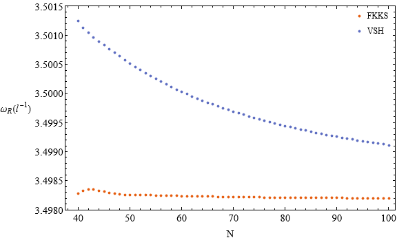
(a) The frequency $\omega_{R}$, the real part of $\omega$, as a function of $N$.

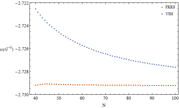
(b) The frequency $\omega_{I}$, the imaginary part of $\omega$, as a function of $N$.

Figure 1: Quasinormal mode of the scalar-type polarization of the Proca field for $\ell=1$, $\mu l=0.50$, $r_{+}=l$ computed with varying computational number $N$, for the VSH method (blue) and the FKKS method (orange). The values in blue seem to converge to the values of orange.

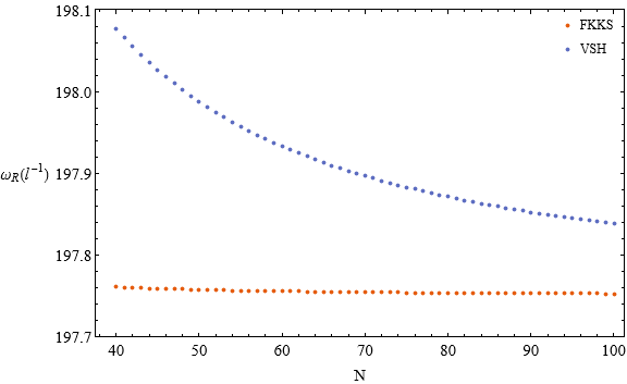
(a) The frequency $\omega_{R}$, the real part of $\omega$, as a function of $N$.

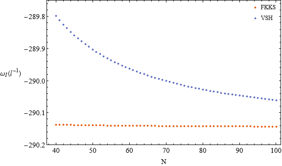
(b) The frequency $\omega_{I}$, the imaginary part of $\omega$, as a function of $N$.

Figure 2: Quasinormal mode of the scalar-type polarization of the Proca field for $\ell=1$, $\mu l=0.50$, $r_{+}=100l$ computed with varying computational number $N$, for the VSH method (blue) and the FKKS method (orange). The values in blue seem to converge to the values of orange.

The value obtained by the VSH method seems to converge to the value obtained by the FKKS method. Even though the value corresponding to the FKKS method also changes, this change only occurs in the fifth significant digit. It was not possible to compute for higher $N$ since it requires higher machine precision.

References

- (1) R. Ruffini, J. Tiomno, and C. V. Vishveshwara, “Electromagnetic field of a particle moving in a spherically symmetric black hole background”, Lett. Nuovo Cimento 3, 211 (1972).
- (2) V. Cardoso and J. P. S. Lemos, “Quasinormal modes of Schwarzschild anti-de Sitter black holes: Electromagnetic and gravitational perturbations”, Phys. Rev. D 64, 084017 (2001); arXiv:gr-qc/0105103.
- (3) V. Cardoso, R. A. Konoplya, and J. P. S. Lemos, “Quasinormal frequencies of Schwarzschild black holes in anti-de Sitter spacetimes: A complete study on the overtone asymptotic behavior”, Phys. Rev. D 68, 044024 (2003); arXiv:gr-qc/0305037.
- (4) M. Wang, C. Herdeiro, and M. O. P. Sampaio, “Maxwell perturbations on asymptotically anti-de Sitter spacetimes: Generic boundary conditions and a new branch of quasinormal modes”, Phys. Rev. D 92, 124006 (2015); arXiv:1510.04713 [gr-qc].
- (5) C. H. Chen, H. T. Cho, and A. S. Cornell, “A new (original) set of quasinormal modes in spherically symmetric AdS black hole spacetimes”, Chin. J. Phys. 67, 646 (2020); arXiv:2004.05806 [gr-qc].
- (6) R. A. Konoplya, A. Zhidenko, and C. Molina, “Late time tails of the massive vector field in a black hole background,” Phys. Rev. D 75, 084004 (2007); arXiv:gr-qc/0602047 [gr-qc].
- (7) J. G. Rosa and S. R. Dolan, “Massive vector fields on the Schwarzschild spacetime: Quasinormal modes and bound states”, Phys. Rev. D 85, 044043 (2012); arXiv:1110.4494 [hep-th].
- (8) R. A. Konoplya, “Massive vector field perturbations in the Schwarzschild background: stability and quasinormal spectrum”, Phys. Rev. D 73, 024009 (2006); arXiv:gr-qc/0509026.
- (9) S. A. Teukolsky, “Rotating black holes: Separable wave equations for gravitational and electromagnetic perturbations”, Phys. Rev. Lett. 29, 1114 (1972).
- (10) P. Pani, V. Cardoso, L. Gualtieri, E. Berti, and A. Ishibashi, “Black hole bombs and photon mass bounds,” Phys. Rev. Lett. 109, 131102 (2012); arXiv:1209.0465 [gr-qc].
- (11) H. Witek, V. Cardoso, A. Ishibashi, and U. Sperhake, “Superradiant instabilities in astrophysical systems,” Phys. Rev. D 87, 043513 (2013); arXiv:1212.0551 [gr-qc].
- (12) V. Cardoso, O. J. C. Dias, G. S. Hartnett, M. Middleton, P. Pani, and J. E. Santos, “Constraining the mass of dark photons and axion-like particles through black-hole superradiance,” J. Cosmol. Astropart. Phys. 03 (2018) 043; arXiv:1801.01420 [gr-qc].
- (13) V. P. Frolov and D. Kubizñák, “Higher-dimensional black holes: Hidden symmetries and separation of variables”, Classical Quantum Gravity 25, 154005 (2008); arXiv:0802.0322 [hep-th].
- (14) T. Houri, T. Oota, and Y. Yasui, “Closed conformal Killing-Yano tensor and uniqueness of generalized Kerr-NUT-de Sitter spacetime”, Classical Quantum Gravity 26, 045015 (2009); arXiv:0805.3877 [hep-th].
- (15) V. P. Frolov, P. Krtouš, and D. Kubizñák, “New metrics admitting the principal Killing–Yano tensor”, Phys. Rev. D 97, 104071 (2018); arXiv:1712.08070 [gr-qc].
- (16) V. P. Frolov, P. Krtouš, and D. Kubizñák, “Black holes, hidden symmetries, and complete integrability”, Living Rev. Relativity 20, 6 (2017); arXiv:1705.05482 [gr-qc].
- (17) O. Lunin, “Maxwell’s equations in the Myers-Perry geometry”, J. High Energy Phys. 12 (2017) 138; arXiv:1708.06766 [hep-th].
- (18) V. P. Frolov, P. Krtouš, D. Kubizñák, and J. E. Santos, “Massive vector fields in rotating black hole spacetimes: Separability and quasinormal modes”, Phys. Rev. Lett. 120, 231103 (2018); arXiv:1804.00030 [hep-th].
- (19) S. R. Dolan, “Instability of the Proca field on Kerr spacetime”, Phys. Rev. D 98, 104006 (2020); arXiv:1806.01604 [gr-qc].
- (20) D. Baumann, H. S. Chia, J. Stout, and L. Haar, “The spectra of gravitational atoms”, J. Cosmol. Astropart. Phys. 12 (2019)006; arXiv:1908.10370 [gr-qc].
- (21) J. Percival and S. R. Dolan, “Quasinormal modes of massive vector fields on the Kerr spacetime”, Phys. Rev. D 102, 104055 (2020); arXiv:2008.10621 [gr-qc].
- (22) G. T. Horowitz and V. E. Hubeny, “Quasinormal modes of AdS black holes and the approach to thermal equilibrium”, Phys. Rev. D 62, 024027 (2000); arXiv:hep-th/9909056.
- (23) V. Cardoso and J. P. S. Lemos, “Scalar, electromagnetic and Weyl perturbations of BTZ black holes: Quasinormal modes”, Phys. Rev. D 63, 124015 (2001); arXiv:gr-qc/0101052.
- (24) T. Delsate, V. Cardoso, and P. Pani, “Anti de Sitter black holes and branes in dynamical Chern-Simons gravity: perturbations, stability and the hydrodynamic modes”, J. High Energy Phys. 06 (2011) 055; arXiv:1103.5756 [hep-th].
- (25) T. V. Fernandes, Vector Fields and Black Holes, M.Sc. Thesis (Instituto Superior Técnico, Lisbon, 2020).