Dynamic Graph Learning-Neural Network for Multivariate Time Series Modeling

Abstract

Multivariate time series forecasting is a challenging task because the data involves a mixture of long- and short-term patterns, with dynamic spatio-temporal dependencies among variables. Existing graph neural networks (GNN) typically model multivariate relationships with a pre-defined spatial graph or learned fixed adjacency graph. It limits the application of GNN and fails to handle the above challenges. In this paper, we propose a novel framework, namely static- and dynamic-graph learning-neural network (SDGL). The model acquires static and dynamic graph matrices from data to model long- and short-term patterns respectively. Static matrix is developed to captures the fixed long-term association pattern via node embeddings, and we leverage graph regularity for controlling the quality of the learned static graph. To capture dynamic dependencies among variables, we propose dynamic graphs learning method to generate time-varying matrices based on changing node features and static node embeddings. And in the method, we integrate the learned static graph information as inductive bias to construct dynamic graphs and local spatio-temporal patterns better. Extensive experiments are conducted on two traffic datasets with extra structural information and four time series datasets, which show that our approach achieves state-of-the-art performance on almost all datasets.

Introduction

Multivariate time series forecasting has great applications in the fields of economics (Qin et al. 2017), geographic (Liang et al. 2018) and traffic (Yu, Yin, and Zhu 2018). The challenge in the task is how to capture the interdependencies and dynamic evolutionary patterns among variables (Peng et al. 2020). Recently, spatio-temporal graph neural networks (GNN) have received increasing attention in modeling temporal data due to high capability in dealing with relational dependencies (Wu et al. 2020).

Presently, most GNN methods are performed on data with a pre-defined graph structure (Guo et al. 2019; Zheng et al. 2020; Song et al. 2020). And now how to get the optimal graph structure becomes the latest research direction of GNN. Graph WaveNet (Wu et al. 2019) captures the hidden spatial dependencies by developing an adaptive dependencies matrix. IDGL (Chen, Wu, and Zaki 2020) finds the optimal graph structure by iteratively updating node embeddings and graph structures. The methods only work best with a well predefined graph. While in most multivariate time series data, the relationships between variables must be discovered from data, rather than provided as priori knowledge. MTGNN (Wu et al. 2020) firstly study graph learning on multivariate time series without a priori structure.

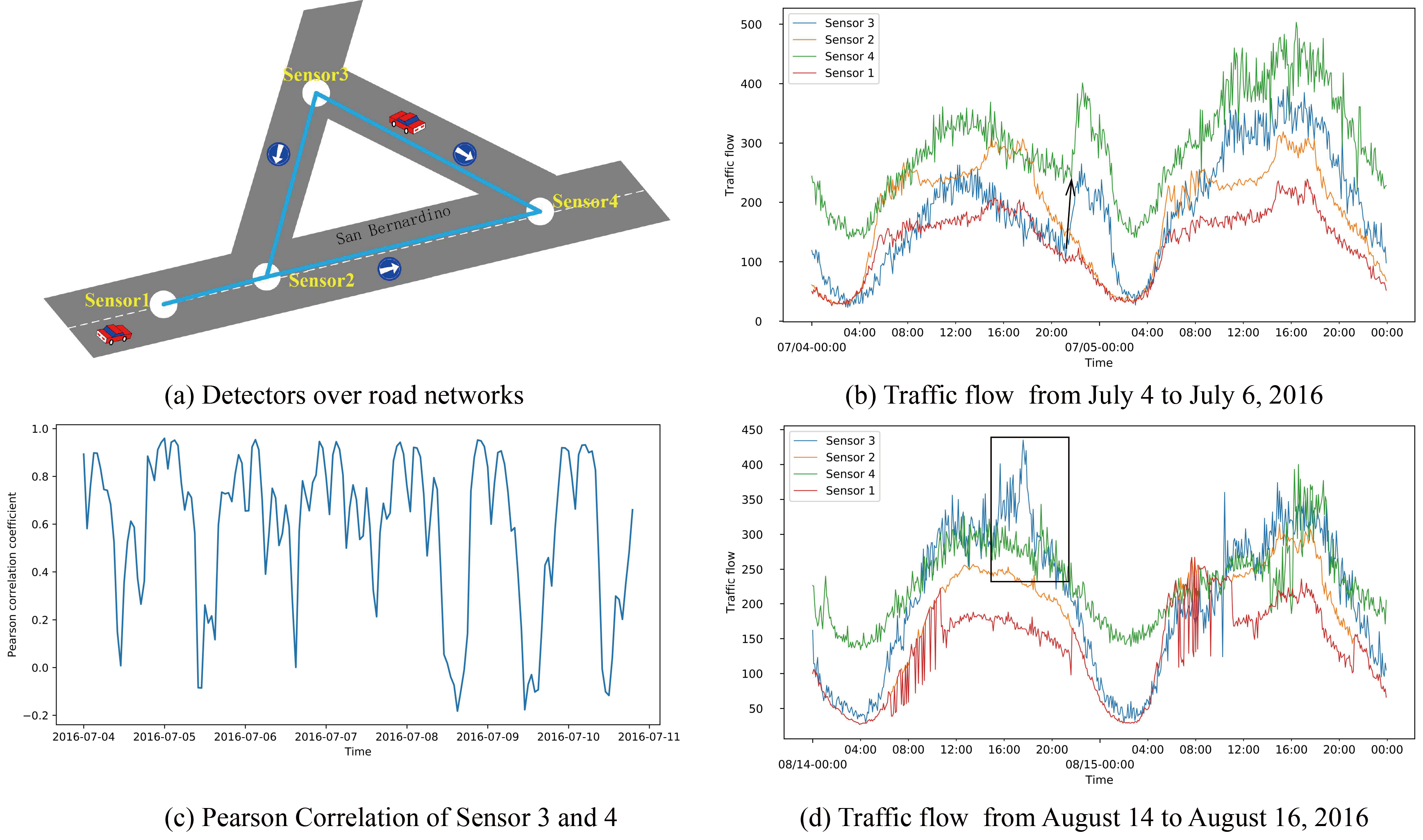
Figure 1: Example of spatial-temporal dependencies in PeMSED8 dataset. (a) Practical location of the four sensors. (b) The traffic flow of sensor 4 is correlated to that of sensor 3, as shown by the black arrow. (c) Pearson Correlation coefficients for sensor 3 and 4. (d) Sudden events, as shown by the balck box

The above methods seek a fixed graph structure, which cannot model spatial-temporal dependencies among variables explicitly and dynamically. Specifically, real-world applications often involve a mixture of long-term and short-term patterns. From Figure 1(a) and Figure 1(b), we can see that long-term correlation of data is dominated by the road network. Figure 1(c) indicates that there exist long-term patterns between sensors 3 and 4, but the short-term correlations between them are changing. Furthermore, there are sudden events, as shown in Figure 1(d). These factors lead to dynamic changes in spatial-temporal dependencies among variables, so the dependencies graph structure should be time-variant and reflect the interaction of patterns. In summary, GNN methods for multivariate time series modeling are facing the following challenges:

• Challenge 1: Interactions of long- and short-term patterns.

• Challenge 2: Dynamic spatial-temporal dependencies among variables.

In this paper, we propose a novel approach to overcome these challenges. For challenge 1, our approach learns two types of graph matrices from data, namely static and dynamic graph matrices. Static graph is used to capture long-term patterns of data, in which we control the learning direction of graph through graph regularity. Dynamic graphs are taken to exact short-term patterns based on static graph, where static graph is constant and dynamic graphs are changing based on node-level data.

For challenge 2, we propose a dynamic graph learning approach to capture varying dependencies between variables. To capture the influence of long- and short-term patterns on inter-variate dependencies, we first utilize a gating mechanism to fuse both learned static patterns and dynamic input. On the basis, we design a multi-headed adjacency mechanism to efficiently extract the associations. To better model local changes, we add long-term patterns as inductive bias, which ensures that dynamic graphs fluctuate up and down around the long-term patterns. In summary, our main contributions are as follows:

• We propose a new graph learning framework to model the interaction of long- and short-term patterns of data, where static graph captures long-term pattern and dynamic graphs are used to model time-varying short-term patterns.

• We design a dynamic graph learning method to efficiently dynamic capture spatial-temporal dependencies among variables, which mine the evolution of associations from data.

• Experiments are conducted on two traffic datasets with predefined graph structures and four benchmark time series datasets. The results demonstrate that our method achieves state-of-the-art results on traffic datasets and most time series datasets without any prior knowledge.

Related Works

Time series forecasting has been studied for a long time. ARIMA(Li and Hu 2012) is a classical statistical method, while it cannot capture nonlinear relationships of data. GP (Frigola 2015) make strong assumptions with respect to a stationary process and cannot scale well to multivariate time series data. Deep-learning-based methods can effectively capture non-linearity of data. Many of them employed convolutional neural networks (CNN) to exact dependencies between variables (Ma et al. 2019; Sen, Yu, and Dhillon 2019). However, CNN cannot take full advantage of the dependencies between pairs of variables. Attention mechanisms are used in time series modeling (Huang et al. 2019) due to the ability to learn feature weights adaptively. However, it models temporal and spatial correlations separately, cannot fully exploit dependencies between variables.

Graph neural networks(GNN) have enjoyed success in handling dependencies among entities, where most methods assume that a well-defined graph already exists (Kipf and Welling 2016; Veličković et al. 2017). Now, researchers work to discover the optimal graph structure from data to improve the performance of GNN (Wu et al. 2019). AM-GCN (Wang et al. 2020) compensates for the limitations of predefined graph by producing a new feature graph. GCNN (Diao et al. 2019) proposed a dynamic matrix estimator to track the spatial dependencies of data. However, the method requires pre-training of the Tensor Decomposition Layer. STFGNN (Li and Zhu 2021) proposed a ”temporal graph” approach to compensate for existing correlations. The method requires prior construction of the ”temporal graph” and an additional operation to obtain spatial-temporal dependencies of data. The performance of the above methods is heavily relying on the quality of prior graph.

Preliminaries

Let $x^{t}\in\mathbb{R}^{N}$ denote the value of a multivariate variable of dimension $N$ at time step $t$, where $x^{t}[i]\in\mathbb{R}$ denotes the value of $i^{th}$ variable at time step $t$. Given a sequence of historical $H$ time steps of observations on a multivariate variable, $X={\{x^{t_{1}},x^{t_{2}},...,x^{t_{h}}\}}=\{x_{1},x_{2},...,x_{N}\}\in\mathbb{R}^{N\times h}$, our goal is to predict the $L$-step-away value of $Y={\{x^{t_{h+L}}\}}$, or a sequence of future values $Y={\{x^{t_{h+1}},x^{t_{h+2}},...,x^{t_{h+L}}\}}$. We aim to build a mapping $f(.)$ from $X$ to $Y$, ie., $Y=f(X)$.

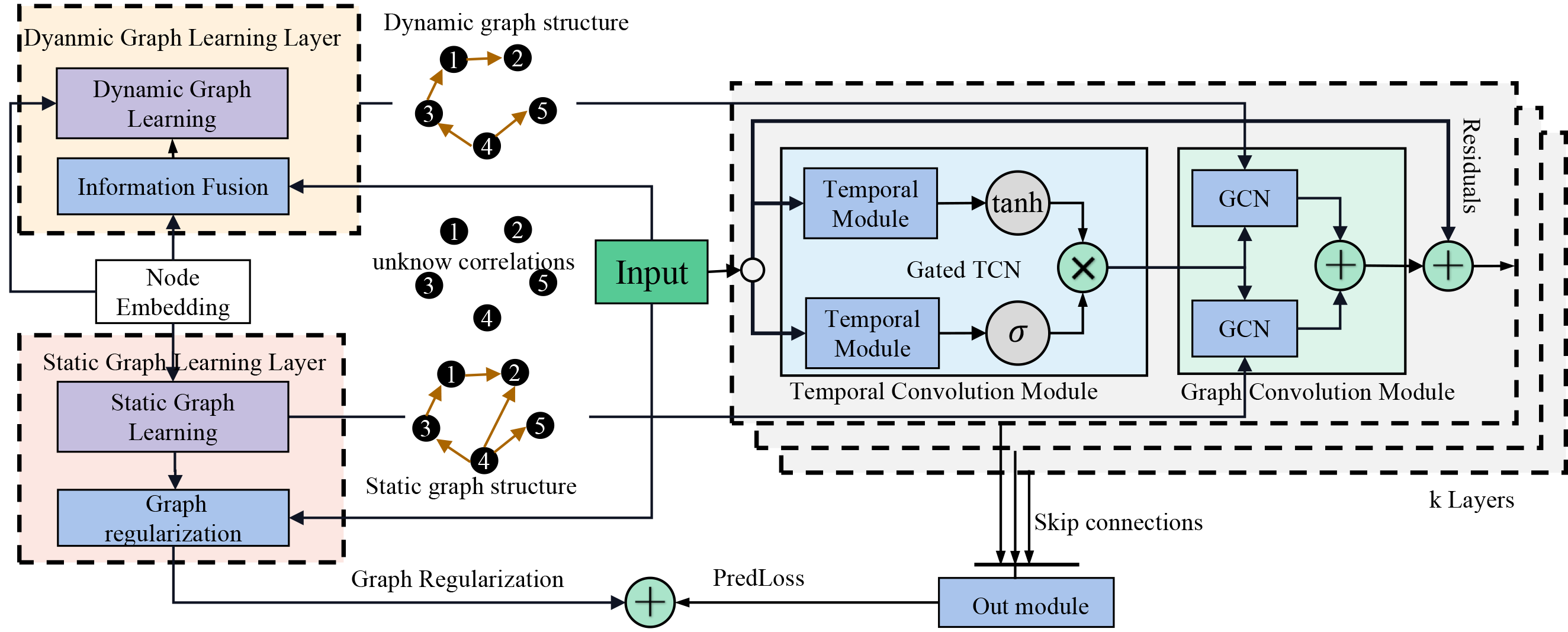
Figure 2: The framework of SDGL. The model consists of static-, dynamic- graph learning layer, temporal convolution (TCN) and graph convolution module (GCN). Input is first passed through graph learning layers to obtain the graph structure. Then input and graphs go through the k-layer TCN and GCN for feature transformation. Finally, the graph regularization and predicted loss are the final loss.

Framework of SDGL

We first elaborate on the general framework of our model. As illustrated in Figure 2, SDGL on the highest level consists of static and dynamic graph learning layers, temporal convolution (TCN), graph convolution modules (GCN), and an output module. To discover the hidden dependencies between variables, two graph learning layers generate two kinds of adjacency matrices, i.e., static and dynamic matrices. TCN adopts a gated structure, which consists of two parallel temporal modules, to extract the temporal dependencies. In GCN, we use two separate modules to aggregate information based on learned static and dynamic matrices. Figure 2 shows how the each module collaborates with each other. In more detail, the core components of our model are illustrated in the following.

Static Graph Learning Layer

Follow previous work (Bai et al. 2020; Wu et al. 2020), we employ node embeddings to capture fixed associations in the data, independent of the dynamic node-level input. The difference is that we add graph regularity to control the learning direction during training, which makes the learned graphs have better convergence and interpretability.

Static Graph Learning: In static graph learning, we first randomly initialize a learnable node embeddings dictionary $M_{s}\in\mathbb{R}^{N\times d}$, where $d$ is the dimension of node embeddings. Then we infer the dependencies between each pair of nodes by Eq.(1).

$$\hat{A}=SoftMax(ReLU(M_{s}\cdot{M_{s}}^{\top}))$$ (1)

We use ReLU activation function to eliminate weak connections. Softmax function is used to normalize the adaptive matrix.

Graph Regularization: It is important to control the smoothness, connectivity and sparsity of learned graph, so we add graph regularization (Jiang et al. 2019) to control the quality of resulting graph. We first apply regularization to dynamic datasets to control graph learning direction. And instead of applying regularization to all inputs at once, we apply it to the data in the gradient update section each time. Given input $X=(x_{1},x_{2},...,x_{N})\in\mathbb{R}^{N\times h}$ and $\hat{A}$, the regularization formula is as follows:

$$L_{GL}=\sum_{i,j=1}^{N}{\parallel x_{i}-x_{j}\parallel}_{2}^{2}\hat{A}+\gamma\parallel\hat{A}\parallel_{F}^{2}$$ (2)

It can be seen that minimizing the first term forces adjacent nodes to have similar features, thus enforcing smoothness of the graph signal on the graph associated with $\hat{A}_{ij}$. The first term in Eq.(2) only requires time window length $H$ data $X$, but during the training, all data in training set affect $\hat{A}$. Eventually, the $\hat{A}_{ij}$ is given a large value if only $x_{i}$ and $x_{j}$ are similar throughout the time range covered by the training set, which ensures that static graph captures long-term dependencies among variables. The second term, where $\parallel\hat{A}\parallel_{F}^{2}$ denotes the Frobenius norm of the matrix, controls sparsity by penalizing large degrees due to the first term in Eq.1.

Dynamic Graph Learning Layer

In multivariate time series data, the dependencies between variables are dynamically changing, which are affected by both fixed graph structure and dynamic inputs, e.g., traffic congestion upstream will gradually affect traffic downstream over time. Different current methods that only exploit graph structure (Wu et al. 2020) or dynamic inputs (Li and Zhu 2021) to get a fixed matrix, we design a dynamic graph learning layer (DGLL) which accounts for both information and dynamically capture spatial-temporal associations between variables. We first fuse the graph structure and input information using designed Information Fusion module. Then we propose Dynamic Graph learning Module to dynamically generate matrices based on fusion results. Due to short-term patterns tend to be locally changing, we add learned fixed patterns as induction bias.

Information Fusion module

To adaptively fuse the fix graph and dynamic inputs, we apply a gated mechanism (Cho et al. 2014). Given the node embeddings $M_{s}\in\mathbb{R}^{N\times d}$ and input $X$. We firstly use a linear layer to transform $X$ to $X_{T}$ which has the same dimension as $M_{s}$. Then information fusion formula is as follows:

$$r_{T}=\delta(W_{r}\cdot M_{s}+U_{r}\cdot X_{T})$$

$$z_{T}=\delta(W_{z}\cdot M_{s}+U_{z}\cdot X_{T})$$

$$\hat{h}_{T}=tanh(W_{h}\cdot X_{T}+r_{T}{(U_{h}\cdot M_{s})})$$

$$h_{T}=(1-z_{T})\cdot M_{s}+z_{T}\cdot\hat{h_{T}}$$ (3)

Where $W$ and $U$ in Eq.(3) are weight matrices need be updated. Then we get result $h_{T}\in\mathbb{R}^{N\times d}$.

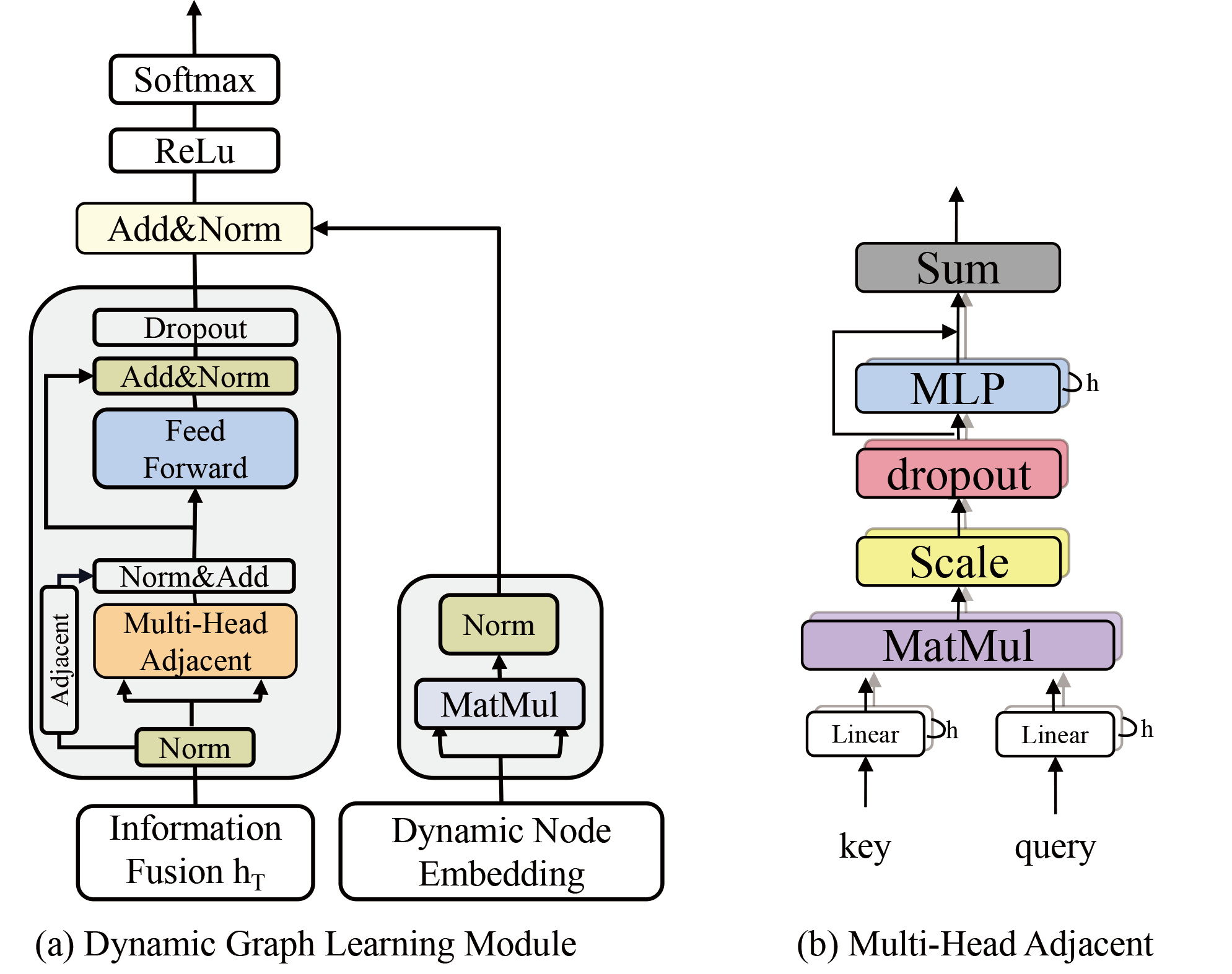
Figure 3: The framwork of Dynamic Graph Learning Module

Dynamic Graph Learning Module

To effectively capture dynamic short-term dependencies between variables, we design dynamic graph learning module (DGLM) that directly produces associations matrices according to the fusion result. As shown in Figure 3(a), DGLM consists of two main components: dynamic matrix construction on the left and inductive bias on the right. The framework of DGLM is inspired by self-attention (Vaswani et al. 2017), but differs from self-attention, our goal is to construct the association matrices between nodes. And we add fixed structure information as inductive bias instead of self-attention without any prior assumptions, which can model spatial-temporal dependencies faithfully.

Dynamic relationship construction: The input $h_{T}$ is first passed through a layer normalization in order to train the model easier(Xiong et al. 2020). We adopt a multi-head way to construct a matrix to capture correlations among variables from multiple perspectives, as shown in Figure 3(b). We project $Q$, $K$ with $W_{q}$ and $W_{k}$ linear projections onto the $d_{k}$, $d_{k}$ dimensions $head$ times, where $K$ and $Q\in\mathbb{R}^{N\times head\times d_{k}}$. Then we perform matrix computation in parallel on each projected version of $Q$, $K$ and produce $head$ matrices, where we adopt scaled dot-product to compute the correlation between $v_{i}$ and $v_{j}$.

$$Adj_{{v_{i}},{v_{j}}}^{head_{i}}=dropout(\frac{Q_{head_{i}}{K_{head_{i}}^{\top}}}{\sqrt{d_{k}}})$$ (4)

In Eq.(4), we added dropout to improve generalization performance of model, as shown in Figure 3(b). Then we projected by a linear layer to get $head_{i}=W_{h}Adj_{v_{i},v_{j}}^{head_{i}}$. Finally the multi-head matrices are summed to get $R_{T}\in\mathbb{R}^{N\times N}$,

$$R_{T}=Sum(head_{1},...,head_{n}),$$ (5)

To avoid that output $R_{T}$ converges to a rank-1 matrix (Dong, Cordonnier, and Loukas 2021), we add skip connection and multi-layer perceptrons (MLPs). We do dot-product using $E_{r}\in\mathbb{R}^{N\times d_{k}}$, where $E_{r}=W_{r}h_{T}$, as residual connection as in Eq.(6), where $LN$ denotes LayerNorm. Then we exploit MLPs to feature projection, as shown in Eq.(7).

$$S_{T}=LN(R_{T})+LN(E_{r}\cdot{E_{r}}^{\top})\\$$ (6)

$$\hat{S}_{T}=max(0,S_{T}W_{1}+b_{1})W_{2}+b_{2}$$ (7)

Inductive bias: Spatial-temporal dependencies in short-term patterns tends to locally change, e.g. peak period traffic patterns tend to be variable but related to road structure. To reflect such trends, we add induction bias, as shown in Eq.(8).

$$A_{d}^{T}=Softmax(Relu(LN(M_{d}\cdot{M_{d}}^{\top})+\hat{S}_{T}))$$ (8)

where $M_{d}\in\mathbb{R}^{N\times d_{k}}$ is dynamic node embeddings, from Eq.(9). The dot result of $M_{d}$ provides fixed structure information for dynamic matrices. Details of $M_{d}$ are shown below.

Momentum update: Our graph structure learning method relies on node embeddings, so the quality of it is crucial. To learn static and dynamic matrices jointly and avoid the opposite effect of two types of graph structures on the same node embeddings, we use two independent node embeddings. Also to ensure the association of dynamic node embeddings with static node embeddings, we introduced momentum update (He et al. 2020). The update equation is shown below.

$$M_{d}\leftarrow pM_{d}+(1-p)M_{s}$$ (9)

Here $p\in[0,1)$ is a momentum coefficient. Only the parameters $M_{s}$ are updated by back-propagation. The process of dynamic graph learning is shown in Algorithm 1.

Algorithm 1 Dynamic Graph Learning

Input: $X\in\mathbb{R}^{N\times h}$
Parameter: node embeddings $M_{s}\in\mathbb{R}^{N\times d_{k}},M_{d}\in\mathbb{R}^{N\times d_{k}}$
Output: dynamic graph $A_{d}^{T}$

1:  $h_{T}\leftarrow X$ and $M_{s}$ using Eq.(3) {get fusion result of $T$}

2:  $Q$, $K$, $E_{r}\leftarrow h_{T}$ by linear layer

3:  $R_{T}\leftarrow\{Q,K\}$ using Eq.(4) and Eq.(5)

4:  $\hat{S}_{T}\leftarrow\{R_{T},E_{r}\}$ using Eq.(6) and Eq.(7)

5:  $A_{d}^{T}\leftarrow\{\hat{S_{T}},M_{d}\}$ using Eq.(8) {add inductive bias}

6:  return $A_{d}^{T}$

Temporal Convolution Module

In temporal convolution module, we take a cnn-based method for the benefits of parallel computing, stable gradients. As shown in Figure 2, we employ gating mechanism (Dauphin et al. 2017), dilated convolutions (van den Oord et al. 2016) and inception (Szegedy et al. 2015). We let the dilation factor for each layer increase exponentially at a rate of $q$ ($q>1$). Suppose the initial factor is 1 and $m$ 1D convolution layers of kernel size $c$, the receptive field of $k$ layer dilated convolutional network is:

$$R=1+(c-1)(q^{k}-1)/(q-1)$$ (10)

In the work, inception layer consisting of four filter sizes, viz. $1\times 2$, $1\times 3$, $1\times 6$, $1\times 7$, which the largest kernel size is used for the calculation the receptive field. Given a 1D sequence input $x\in\mathbb{R}^{T}$ and filters consisting of $f_{1\times 2}\in\mathbb{R}^{2}$, $f_{1\times 3}\in\mathbb{R}^{3}$, $f_{1\times 6}\in\mathbb{R}^{6}$, $f_{1\times 7}\in\mathbb{R}^{7}$, the dilated inception layer takes the form Eq.(11).

$$H=concat(H*f_{1\times 2},H*f_{1\times 3},H*f_{1\times 6},H*f_{1\times 7})$$ (11)

Where the outputs of the four filters are truncated to the same length according to the largest filter and concatenated across the channel dimension. And the dilated convolution denoted by $H*f_{1\times r}$ is defined as $H*f_{1\times r}(t)=\sum_{s=0}^{r-1}f_{1\times r}(s)H(t-d\times s)$, where d is the dilation factor.

Graph Convolution Module

The graph convolution module aims to fuse node’s with its neighbors’ features to obtain new node representation. Li et al. modeled diffusion process of graph signals with $S$ finite steps (Li et al. 2018). Let $A\in\mathbb{R}^{N\times N}$ denote the adjacency matrix, $X\in\mathbb{R}^{N\times D}$ denote the input, $Z\in\mathbb{R}^{N\times M}$ denotes result and $W_{s}\in\mathbb{R}^{D\times M}$ denote model parameters. The form can be generalize into $Z=\sum_{s=0}^{s}P^{s}XW_{s}$, where $P^{s}\in\mathbb{R}^{N\times N}$ represents the power series of transition matrix. In the case of an graph, $P=A/rowsum(A)$.

We decouple the information propagation and representation transformation operations (Liu, Gao, and Ji 2020) and exploit the $W_{s}$ as the information selection layer, with the following equation:

$$Z=W_{s}concat(P^{1}X,...P^{s}X,X)$$ (12)

where $W_{s}$ implemented with $1\times 1$ convolutional, with the input channel $c(s+1)$ and output channel $c$. In the extreme case, i.e., where there is no dependence among variables, aggregating information just adds noise to each node. So, we use $W_{s}$ to select the significant information generated at each transition matrix. In above case, Eq.(12) still preserves nodes’ own information by adjusting $W_{s}$ to 0 for $P^{1}X,...P^{s}X$.

To model the interaction of short-term and long-term patterns, we adopt two graph convolution layers to capture node information on static and dynamic graphs separately, that is, replacing A with learned $\hat{A}$ and $A_{d}^{T}$. The final output is shown in Eq.(13).

$$Z_{f}=Z_{static}+Z_{dynamic}$$ (13)

Joint Learning with A Hybrid Loss

In contrast to previous work that optimizes the adjacency matrix based on task-related prediction loss, we jointly learn the graph and GNN parameters by minimizing a hybrid loss that combines prediction and graph regularization loss.

The full process of SDGL is shown in Algorithm 2. As we can see, our framework only needs to initialize node embeddings $M_{s}$. Then we construct static graph based on $M_{s}$ (Eqs. (1)), and dynamic graphs are generated using Algorithm 1. The input $X$ and learned graphs are subjected to feature extraction and aggregation by TCN and GCN (Eq.(11) and Eq.(13)). Finally, we update parameters of model according to hybrid loss $L_{loss}$, while updating the $M_{d}$ using momentum update (Eq. (9)).

Algorithm 2 General Framework of SDGL

Input: The dataset $O$
Parameter: $M_{s}$, $M_{d}$, $H$, $L$, $iter$, $K$, $B$, $epoch$
Output: prediction value $\hat{Y}$

1:  init node embeddings and $M_{d}\leftarrow M_{s}$

2:  for $r$ in $1:epoch$ do

3:     for $i$ in $1:iter$ do

4:        Sample $X\in R^{B\times N\times H}$, $Y\in R^{B\times N\times L}$ from $O$

5:        calculate received filed using Eq.(10)

6:        $\hat{A}\leftarrow\{M_{s}\}$ using Eq.(1)

7:        $L_{GL}\leftarrow\{\hat{A},X\}$ using Eq.(2)

8:        $A_{d}^{T}\leftarrow\{M_{s},M_{d},X\}$ using Algorithm.(1)

9:        for $j$ in $1:K$ do

10:           $H^{j}\leftarrow\{X\}$ using Eq.(11)

11:           $Z_{f}^{j}\leftarrow\{H^{j},\hat{A},A_{d}^{T}\}$ using Eq.(13)

12:           $X\leftarrow Z_{f}^{j}$ and $output+=H^{j}$

13:        end for

14:        $\hat{Y}\leftarrow\{output\}$ using output module

15:        $L_{loss}\leftarrow\lambda L_{GL}+L1loss(\hat{Y},Y)$

16:        Back-propagate $L_{loss}$ update model paramters and $M_{d}$ using Eq.(9), $i\leftarrow i+1$

17:     end for

18:     $r\leftarrow r+1$

19:  end for

Experiments

To evaluate the performance of SDGL, we conduct experiments on two tasks single-step and multi-step forecasting. First, to illustrate how well SDGL performs, we evaluate it on two public traffic datasets (Bai et al. 2020), compared to other spatio-temporal graph neural networks, where the aim is to predict multiple future steps. Then, we compare the SDGL with other multivariate time series models on four benchmark datasets, where the aim is to predict a single future step (Wu et al. 2020).

Dataset and Experimental Setting

Datasets	Samples	Nodes	Input_len	Pred_len
PeMSD4	16992	307	12	12
PeMSD8	17856	170	12	12
Traffic	17544	862	168	1
Solar-energy	52560	137	168	1
Electricity	26304	321	168	1
Exchange-rate	7588	8	168	1

Table 1: Dataset statistics

In Table 1, we summarize the statistics of benchmark datasets. In Multi-step prediction experiment, following the method (Bai et al. 2020), we use three evaluation metrics, i.e., MAE, MAPE and RMSE. In Single-step prediction experiment, we use Root Relative Squared Error (RSE), and Coefficient Correlation (CORR) to measure the performance of predictive models (Wu et al. 2020). The specific calculation formula is detailed in Appendix A.2. For RMSE, MAE, MAPE and RRSE, lower the values are better. For CORR, higher the values are better.

Baseline Methods for Comparision

Multi-step forecasting

• HA: Historical Average, which uses the average of previous seasons as the prediction.

• VAR (Zivot and Wang 2006): Vector Auto-Regression:a model that captures correlations among traffic series.

• DSANet (Huang et al. 2019): A prediction model using CNN networks and self-attention mechanism.

• DCRNN (Li et al. 2018): A diffusion convolutional recurrent neural network containing graph convolution.

• STGCN (Yu, Yin, and Zhu 2018): A spatial-temporal GNN.

• ASTGCN (Guo et al. 2019): Attention-based spatio-temporal GNN, which integrates spatial and temporal attention mechanisms.

• STSGCN (Song et al. 2020): Spatial-temporal GNN that captures correlations by stacking multiple localized GCN layers with adjacent matrix over the time axis.

• AGCNR (Bai et al. 2020): Adaptive Graph Convolutional Recurrent Network that capture association of data and node-specific patterns through node embeddings.

Single-step forecasting

• AR: Auto-regressive model, a statistical model.

• VAR-MLP (Zhang 2003): A hybrid model of the multilayer perception and auto-regressive model.

• GP (Frigola 2015) A Gaussian Process time series model.

• RNN-GRU: A recurrent neural network with fully connected GRU hidden units.

• LSTNet (Lai et al. 2018): Long- and Short-term Time-series network, which uses the CNN and Recurrent Neural Network to extract short-term patterns and to discover long-term patterns for time series trends.

• TPA-LSTM (Shih, Sun, and Lee 2019): Temporal pattern attention network that capture patterns across time steps.

• MTGNN (Wu et al. 2020): The first study on multivariate time series from a graph-based perspective with GNN.

Main Results

Multi-step forecasting

Dataset	Metric	HA	VAR	GRU-ED	DSANet	DCRNN	STGCN	ASTGCN	STSGCN	AGCNR	SDGL
	MAE	38.03	24.54	23.68	22.79	21.22	21.16	22.93	21.19	19.83	18.65
PeMSD4	MAPE(%)	27.88	17.24	16.44	16.03	14.17	13.83	16.56	13.9	12.97	12.38
	RMSE	59.24	38.61	39.27	35.77	33.44	34.89	35.22	33.65	32.26	31.30
	MAE	34.86	19.19	22	17.14	16.82	17.5	18.25	17.13	15.95	14.93
PeMSD8	MAPE(%)	24.07	13.1	13.33	11.32	10.92	11.29	11.64	10.96	10.09	9.61
	RMSE	52.04	29.81	36.23	26.96	26.36	27.09	28.06	26.86	25.22	24.13

Table 2: Baseline comparison under multi-step forecasting for spatial-temporal graph neural networks.

Table 2 and Table 3 provide the main experimental results of SDGL. We observe that our model achieves state-of-the-art results on most of tasks, with on-par performance comparable to the state-of-the-art in the remaining tasks. In the following, we discuss experimental results of multi-step and single-step forecasting respectively.

Multi-step forecasting

Table 2 presents the overall prediction performances, which are the averaged MAE, RMSE and MAPE over 12 prediction horizons, of our SDGL and night representative comparison methods. We can observe that: 1) GCN-based methods outperform baselines and self-attention-based DSANet, demonstrating the effectiveness of GCN in traffic time series forecasting. 2) The performance of the graph-learned method performs better than that of using predefined graphs. AGCNR significantly improves the performance of GCN-based method based on learned dependencies. 3) Our method further improves learning-graph based methods with a significant margin. SDGL brings more than 6% relative improvements to the existing best results in MAE for PeMSD4 and PeMSD8 datasets.

Single-step forecasting

In this experiment, we compare SDGL with other multivariate time series models. Table 3 shows the experimental results for the single-step forecasting task. 1) The performance of the methods that model the relationships between variables show higher performance, i.e., TPA-LSTM, demonstrating the importance of modeling the relationships. 2) GNN-based methods outperform other baseline methods, i.e., MTGNN, indicating that GNN has greater ability to model dependencies between variables. 3) Our approach further improves the performance of GNN-based method, which demonstrates the effectiveness of SDGL. On Solar-Energy and Electricity dataset, the improvement of SDGL in terms of RSE is significant, which SDGL lowers down RSE by more than 4% over the horizons of 3, 6, 12, 24 on the Solar-Energy data. SDGL slightly outperforms MTGNN in traffic data, where MTGNN improves traffic forecasting performance significantly. We conjecture the reason is that the target of the forecast is road occupancy, which the values changes with relatively stable patterns. SDGL improves on CORR metrics for exchange rate data only, but outperforms the graph neural network MTGNN in all metrics.

Dataset		Solar_Energy				Traffic				Electricity				Exchange_Rate
		Horizon				Horizon				Horizon				Horizon
Methods	Metrics	3	6	12	24	3	6	12	24	3	6	12	24	3	6	12	24
AR	RSE	0.2435	0.3790	0.5911	0.8699	0.5991	0.6218	0.6252	0.63	0.0995	0.1035	0.1050	0.1054	0.0228	0.0279	0.0353	0.0445
	CORR	0.9710	0.9263	0.8107	0.5314	0.7752	0.7568	0.7544	0.7519	0.8845	0.8632	0.8591	0.8595	0.9734	0.9656	0.9526	0.9357
VARMLP	RSE	0.1922	0.2679	0.4244	0.6841	0.5582	0.6579	0.6023	0.6146	0.1393	0.1620	0.1557	0.1274	0.0265	0.0394	0.0407	0.0578
	CORR	0.9829	0.9655	0.9058	0.7149	0.8245	0.7695	0.7929	0.7891	0.8708	0.8389	0.8192	0.8679	0.8609	0.8725	0.8280	0.7675
GP	RSE	0.2259	0.3286	0.5200	0.7973	0.6082	0.6772	0.6406	0.5995	0.1500	0.1907	0.1621	0.1273	0.0239	0.0272	0.0394	0.0580
	CORR	0.9751	0.9448	0.8518	0.5971	0.7831	0.7406	0.7671	0.7909	0.8670	0.8334	0.8394	0.8818	0.8713	0.8193	0.8484	0.8278
RNN-GRU	RSE	0.1932	0.2628	0.4163	0.4852	0.5358	0.5522	0.5562	0.5633	0.1102	0.1144	0.1183	0.1295	0.0192	0.0264	0.0408	0.0626
	CORR	0.9823	0.9675	0.9150	0.8823	0.8511	0.8405	0.8345	0.8300	0.8597	0.8623	0.8472	0.8651	0.9786	0.9712	0.9531	0.9223
LSNet-skip	RSE	0.1843	0.2559	0.3254	0.4643	0.4777	0.4893	0.4950	0.4973	0.0864	0.0931	0.1007	0.1007	0.0226	0.0280	0.0356	0.0449
	CORR	0.9843	0.9690	0.9467	0.8870	0.8721	0.8690	0.8614	0.8588	0.9283	0.9135	0.9077	0.9119	0.9735	0.9658	0.9511	0.9354
TPA-LSTM	RSE	0.1803	0.2347	0.3234	0.4389	0.4487	0.4658	0.4641	0.4765	0.0823	0.0916	0.0964	0.1006	0.0174	0.0241	0.0341	0.0444
	CORR	0.9850	0.9742	0.9487	0.9081	0.8812	0.8717	0.8717	0.8629	0.9439	0.9337	0.9250	0.9133	0.9790	0.9709	0.9564	0.9381
MTGNN	RSE	0.1778	0.2348	0.3109	0.4270	0.4162	0.4754	0.4461	0.4535	0.0745	0.0878	0.0916	0.0953	0.0194	0.0259	0.0349	0.0456
	CORR	0.9852	0.9726	0.9509	0.9031	0.8963	0.8667	0.8794	0.8810	0.9474	0.9316	0.9278	0.9234	0.9786	0.9708	0.9551	0.9372
SDGL	RSE	0.1699	0.2222	0.2924	0.4047	0.4142	0.4475	0.4584	0.4571	0.0698	0.0805	0.0889	0.0935	0.0180	0.0249	0.0342	0.0455
	CORR	0.9866	0.9762	0.9565	0.9119	0.9010	0.8825	0.8760	0.8766	0.9534	0.9445	0.9351	0.9301	0.9808	0.9730	0.9583	0.9402

Table 3: Baseline comparison under single-step forecasting for multivariate time series methods.

Ablation Study

We conduct an ablation study on the PeMSD and PeMSD8 datasets to validate the effectiveness of key components that contribute to the improved outcomes of our model. We name SDGL without different components as follows:

• SDGLw/oGLoss: SDGL without Grpah regularization. We set the factors $\lambda$ directly to 0.

• SDGLw/oDyAdj: SDGL without Dynamic graph learning layer.

• SDGLw/o IFM: SDGL without the Information fusion module in Dynamic Graph Learning Layer. We pass the node-level inputs to the dynamic graph learning module, which means consider only dynamic node inputs.

• SDGLw/o IFM +: We replace the information fusion module with a summation operation.

The test results measured using RMSE, MAPE are shown in Figure 4(a), more details are detailed in Appendix A.6. Several observations from these results are worth highlighting:

• The best result on each dataset is obtained with SDGL, proving that each of our modules worked.

• Removing the dynamic graph learning layer (DGLL) causes performance drop, which is obvious in the RMSE for PEMSD4 dataset and MAPE for PEMSD8 dataset. Also after removing the DGLL, the effect gradually deteriorates over time among the 12 prediction steps, as shown in Figure 4(b). We conjecture the reason is that long-term prediction lacks sufficiently useful information from historical observations and thus benefits from the short-term patterns learned by DGLL to deduce future values.

• After removing the IFM module, performance drops when dynamic graph are constructed base on only node-level inputs, especially in the long term (e.g., 60 Min) prediction. Whereas with the + operation instead of information fusion, the performance drops only slightly in all prediction steps. It demonstrates the importance of long-term patterns have significant impacts on inter-variate dependencies.

• The performance drops after removing graph regularization, proving that the regularization improves the quality of learned graph by SDGL. But overall, SDGLw/oGLoss outperformed AGCNR in multi-step prediction on both datasets, except for MAPE in 60-min prediction. It suggests that our proposed static- and dynamic- graph approach itself can improve performance, rather than relying on the addition of graph regularity.

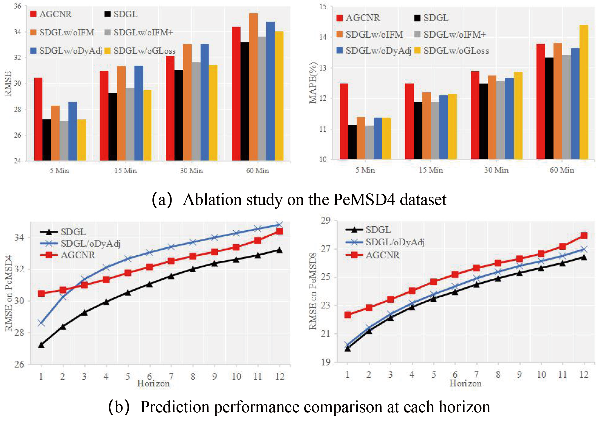
Figure 4: Results of SDGL in the ablation tests

Study of the Graph Learning Layer

To verify the effectiveness of our proposed graph learning method, we visualize and analyze the matrices learned by model. Figure 5 shows the pre-defined graph matrix in PeMSD8 dataset, static graph structure and the dynamic graphs at two different time spans. As shown in Figure 5(b), we observe that in static graph, most of nodes present self-attention, i.e. diagonal line in the figure. In contrast to the manual addition of self-loops in the predefined matrix, self-attention in static graph is acquired by model. Further, we present the dynamic graph matrices at different time spans in Figure 5(c). We find that there are two data points of higher weight in the dynamic graph, which corresponds to exactly two important data points in the predefined graph, i.e., 12 and 28. As shown in Figure 5(c), the heatmaps of the dynamic matrices on the two close time spans are very close to each other, which indicates that the dynamic graphs learn a short-term pattern. The two regions marked with “loc 1” and “loc 2” demonstrate that our model can capture the changes in intervariate dependencies.

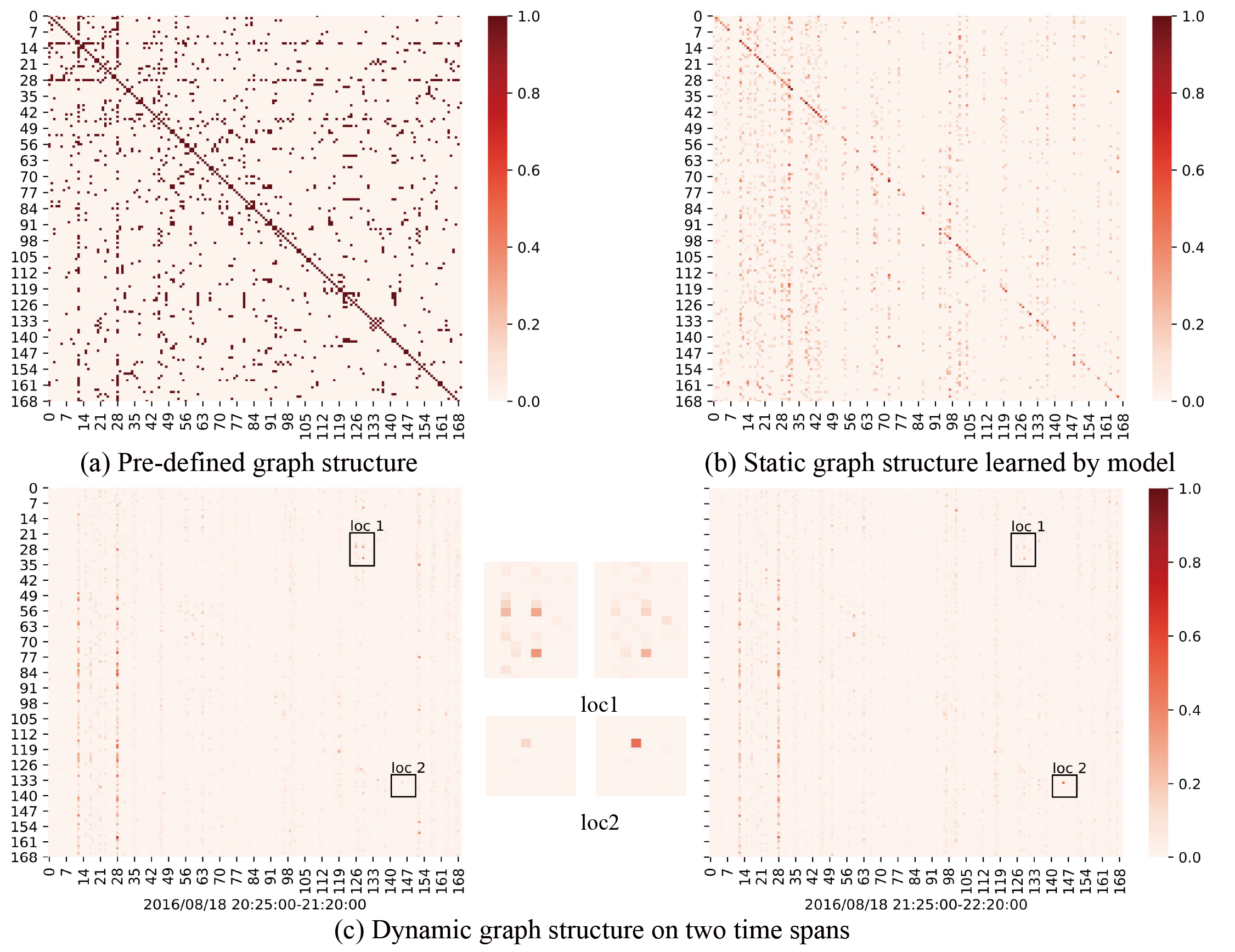
Figure 5: Graph structure visualization

Conclusion

In this paper, we propose a novel graph neural network for multivariate time series forecasting. This work models long- and short-term spatiotemporal patterns in multivariate time series data by constructing static and dynamic graph matrices from data. Also dynamic graphs are generated dynamically based on time-varying inputs and fixed long-term patterns to capture the changing spatial-temporal dependence among variables. Our approach shows excellent performance in both multi-step traffic prediction and single-step time series prediction tasks. It reveals that correctly and adequately modeling the dependencies between pairs of variables is essential for understanding time series data.

References

- Bai et al. (2020) Bai, L.; Yao, L.; Li, C.; Wang, X.; and Wang, C. 2020. Adaptive Graph Convolutional Recurrent Network for Traffic Forecasting. In 34th Conference on Neural Information Processing Systems.
- Chen, Wu, and Zaki (2020) Chen, Y.; Wu, L.; and Zaki, M. 2020. Iterative deep graph learning for graph neural networks: Better and robust node embeddings. Advances in Neural Information Processing Systems, 33.
- Cho et al. (2014) Cho, K.; Gulcehre, B. v. M. C.; Bahdanau, D.; Schwenk, F. B. H.; and Bengio, Y. 2014. Learning Phrase Representations using RNN Encoder–Decoder for Statistical Machine Translation. Computer Sciences.
- Dauphin et al. (2017) Dauphin, Y. N.; Fan, A.; Auli, M.; and Grangier, D. 2017. Language modeling with gated convolutional networks. In International conference on machine learning, 933–941. PMLR.
- Diao et al. (2019) Diao, Z.; Wang, X.; Zhang, D.; Liu, Y.; Xie, K.; and He, S. 2019. Dynamic spatial-temporal graph convolutional neural networks for traffic forecasting. In Proceedings of the AAAI conference on artificial intelligence, volume 33, 890–897.
- Dong, Cordonnier, and Loukas (2021) Dong, Y.; Cordonnier, J.-B.; and Loukas, A. 2021. Attention is not all you need: Pure attention loses rank doubly exponentially with depth. arXiv preprint arXiv:2103.03404.
- Frigola (2015) Frigola, R. 2015. Bayesian time series learning with Gaussian processes. Ph.D. thesis, University of Cambridge.
- Guo et al. (2019) Guo, S.; Lin, Y.; Feng, N.; Song, C.; and Wan, H. 2019. Attention based spatial-temporal graph convolutional networks for traffic flow forecasting. In Proceedings of the AAAI Conference on Artificial Intelligence, volume 33, 922–929.
- He et al. (2020) He, K.; Fan, H.; Wu, Y.; Xie, S.; and Girshick, R. 2020. Momentum contrast for unsupervised visual representation learning. In Proceedings of the IEEE/CVF Conference on Computer Vision and Pattern Recognition, 9729–9738.
- Huang et al. (2019) Huang, S.; Wang, D.; Wu, X.; and Tang, A. 2019. Dsanet: Dual self-attention network for multivariate time series forecasting. In Proceedings of the 28th ACM international conference on information and knowledge management, 2129–2132.
- Jiang et al. (2019) Jiang, B.; Zhang, Z.; Lin, D.; Tang, J.; and Luo, B. 2019. Semi-supervised learning with graph learning-convolutional networks. In Proceedings of the IEEE/CVF Conference on Computer Vision and Pattern Recognition, 11313–11320.
- Kipf and Welling (2016) Kipf, T. N.; and Welling, M. 2016. Semi-supervised classification with graph convolutional networks. arXiv preprint arXiv:1609.02907.
- Lai et al. (2018) Lai, G.; Chang, W.-C.; Yang, Y.; and Liu, H. 2018. Modeling long-and short-term temporal patterns with deep neural networks. In The 41st International ACM SIGIR Conference on Research & Development in Information Retrieval, 95–104.
- Li and Hu (2012) Li, C.; and Hu, J.-W. 2012. A new ARIMA-based neuro-fuzzy approach and swarm intelligence for time series forecasting. Engineering Applications of Artificial Intelligence, 25(2): 295–308.
- Li and Zhu (2021) Li, M.; and Zhu, Z. 2021. Spatial-Temporal Fusion Graph Neural Networks for Traffic Flow Forecasting. In Proceedings of the AAAI Conference on Artificial Intelligence, volume 35, 4189–4196.
- Li et al. (2018) Li, Y.; Yu, R.; Shahabi, C.; and Liu, Y. 2018. Diffusion Convolutional Recurrent Neural Network: Data-Driven Traffic Forecasting. In International Conference on Learning Representations.
- Liang et al. (2018) Liang, Y.; Ke, S.; Zhang, J.; Yi, X.; and Zheng, Y. 2018. Geoman: Multi-level attention networks for geo-sensory time series prediction. In IJCAI, volume 2018, 3428–3434.
- Liu, Gao, and Ji (2020) Liu, M.; Gao, H.; and Ji, S. 2020. Towards deeper graph neural networks. In Proceedings of the 26th ACM SIGKDD International Conference on Knowledge Discovery & Data Mining, 338–348.
- Ma et al. (2019) Ma, Q.; Tian, S.; Wei, J.; Wang, J.; and Ng, W. W. 2019. Attention-based spatio-temporal dependence learning network. Information Sciences, 503: 92–108.
- Peng et al. (2020) Peng, H.; Wang, H.; Du, B.; Bhuiyan, M. Z. A.; Ma, H.; Liu, J.; Wang, L.; Yang, Z.; Du, L.; Wang, S.; et al. 2020. Spatial temporal incidence dynamic graph neural networks for traffic flow forecasting. Information Sciences, 521: 277–290.
- Qin et al. (2017) Qin, Y.; Song, D.; Chen, H.; Cheng, W.; Jiang, G.; and Cottrell, G. 2017. A dual-stage attention-based recurrent neural network for time series prediction. arXiv preprint arXiv:1704.02971.
- Sen, Yu, and Dhillon (2019) Sen, R.; Yu, H.-F.; and Dhillon, I. 2019. Think globally, act locally: a deep neural network approach to high-dimensional time series forecasting. In Proceedings of the 33rd International Conference on Neural Information Processing Systems, 4837–4846.
- Shih, Sun, and Lee (2019) Shih, S.-Y.; Sun, F.-K.; and Lee, H.-y. 2019. Temporal pattern attention for multivariate time series forecasting. Machine Learning, 108(8): 1421–1441.
- Song et al. (2020) Song, C.; Lin, Y.; Guo, S.; and Wan, H. 2020. Spatial-temporal synchronous graph convolutional networks: A new framework for spatial-temporal network data forecasting. In Proceedings of the AAAI Conference on Artificial Intelligence, volume 34, 914–921.
- Szegedy et al. (2015) Szegedy, C.; Liu, W.; Jia, Y.; Sermanet, P.; Reed, S.; Anguelov, D.; Erhan, D.; Vanhoucke, V.; and Rabinovich, A. 2015. Going deeper with convolutions. In Proceedings of the IEEE conference on computer vision and pattern recognition, 1–9.
- van den Oord et al. (2016) van den Oord, A.; Dieleman, S.; Zen, H.; Simonyan, K.; Vinyals, O.; Graves, A.; Kalchbrenner, N.; Senior, A.; and Kavukcuoglu, K. 2016. WaveNet: A Generative Model for Raw Audio. In 9th ISCA Speech Synthesis Workshop, 125–125.
- Vaswani et al. (2017) Vaswani, A.; Shazeer, N.; Parmar, N.; Uszkoreit, J.; Jones, L.; Gomez, A. N.; Kaiser, Ł.; and Polosukhin, I. 2017. Attention is all you need. In Advances in neural information processing systems, 5998–6008.
- Veličković et al. (2017) Veličković, P.; Cucurull, G.; Casanova, A.; Romero, A.; Lio, P.; and Bengio, Y. 2017. Graph attention networks. arXiv preprint arXiv:1710.10903.
- Wang et al. (2020) Wang, X.; Zhu, M.; Bo, D.; Cui, P.; Shi, C.; and Pei, J. 2020. Am-gcn: Adaptive multi-channel graph convolutional networks. In Proceedings of the 26th ACM SIGKDD International conference on knowledge discovery & data mining, 1243–1253.
- Wu et al. (2020) Wu, Z.; Pan, S.; Long, G.; Jiang, J.; Chang, X.; and Zhang, C. 2020. Connecting the dots: Multivariate time series forecasting with graph neural networks. In Proceedings of the 26th ACM SIGKDD International Conference on Knowledge Discovery & Data Mining, 753–763.
- Wu et al. (2019) Wu, Z.; Pan, S.; Long, G.; Jiang, J.; and Zhang, C. 2019. Graph WaveNet for Deep Spatial-Temporal Graph Modeling. In The 28th International Joint Conference on Artificial Intelligence (IJCAI). International Joint Conferences on Artificial Intelligence Organization.
- Xiong et al. (2020) Xiong, R.; Yang, Y.; He, D.; Zheng, K.; Zheng, S.; Xing, C.; Zhang, H.; Lan, Y.; Wang, L.; and Liu, T. 2020. On layer normalization in the transformer architecture. In International Conference on Machine Learning, 10524–10533. PMLR.
- Yu, Yin, and Zhu (2018) Yu, B.; Yin, H.; and Zhu, Z. 2018. Spatio-temporal graph convolutional networks: a deep learning framework for traffic forecasting. In Proceedings of the 27th International Joint Conference on Artificial Intelligence, 3634–3640.
- Zhang (2003) Zhang, G. P. 2003. Time series forecasting using a hybrid ARIMA and neural network model. Neurocomputing, 50: 159–175.
- Zheng et al. (2020) Zheng, C.; Fan, X.; Wang, C.; and Qi, J. 2020. Gman: A graph multi-attention network for traffic prediction. In Proceedings of the AAAI Conference on Artificial Intelligence, volume 34, 1234–1241.
- Zivot and Wang (2006) Zivot, E.; and Wang, J. 2006. Vector autoregressive models for multivariate time series. Modeling Financial Time Series with S-Plus®, 385–429.