Multi-scale Graph Convolutional Networks with Self-Attention

Abstract

Graph convolutional networks (GCNs) have achieved remarkable learning ability for dealing with various graph structural data recently. In general, deep GCNs do not work well since graph convolution in conventional GCNs is a special form of Laplacian smoothing, which makes the representation of different nodes indistinguishable. In the literature, multi-scale information was employed in GCNs to enhance the expressive power of GCNs. However, over-smoothing phenomenon as a crucial issue of GCNs remains to be solved and investigated. In this paper, we propose two novel multi-scale GCN frameworks by incorporating self-attention mechanism and multi-scale information into the design of GCNs. Our methods greatly improve the computational efficiency and prediction accuracy of the GCNs model. Extensive experiments on both node classification and graph classification demonstrate the effectiveness over several state-of-the-art GCNs. Notably, the proposed two architectures can efficiently mitigate the over-smoothing problem of GCNs, and the layer of our model can even be increased to $64$.

Introduction

Graph structural data related learning has drawn considerable attention recently. Graph neural networks (GNNs), particularly graph convolutional networks (GCNs) have been successfully utilized in various fields of artificial intelligence, but not limited to recommendation systems (Sun et al. 2020), computer vision (Casas et al. 2020), molecular design (Stokes et al. 2020), natural language processing (Yao, Mao, and Luo 2019), node classification (Kipf and Welling 2017), graph classification (Xu et al. 2019b), and clustering (Zhu 2012). Despite their great success, existing GCNs has low expressive power and may confront with the problem of over-smoothing, since graph convolution applies the same operation to all the neighbors of node. Therefore, almost all GCNs have shallow structures with only two or three layers. This undoubtedly limits the expressive ability and the extraction ability of high-order neighbors of GCNs.

Several methods try to deal with the over-smoothing issue and deepen the networks. Sun, Lin, and Zhu (2021) developed a novel AdaGCN by incorporating AdaBoost into the design of GCNs. JKNet (Xu et al. 2018) used the information of each layer to improve the predictive ability of graph convolution. Rong et al. (2020) suggested removing a few edges of the graph randomly to mitigate the impact of over-smoothing, whilst Luan et al. (2019) utilized multi-scale information to deepen GCNs.

However, the above-mentioned approaches yield steep increasing of computation due to the accumulation of too many layers, although the structure of GCNs is deepened. In this paper, we propose two general GCN frameworks by employing the idea of self-attention and multi-scale information. On one hand, the introduction of multi-scale information will enhance the expressive ability of GCNs by stacking many layers, which is scalable in depth. On the other hand, the self-attention mechanism will alleviate the over-smoothing problem, and reduce computational cost. Moreover, the proposed frameworks are flexible and can be built on any GCNs model. Extensive comparison against baselines in both node classification and graph classification is investigated. The experimental results indicate significant performance improvements on both graph and node classification tasks over a variety of real-world graph structural data.

Related Work

In general, there are two convolution operations in the model of GCNs: spatial-based method and spectral-based approach. Spatial-based GCNs consider the aggregation method between the graph nodes. GAT (Veličković et al. 2018) used the attention mechanism to aggregate neighboring nodes on the graph, and GraphSAGE (Hamilton, Ying, and Leskovec 2017) utilized random walks to sample nodes and then aggregated them. Spetral-based GCNs focus on redefining the convolution operation by utilizing Fourier transform (Bruna et al. 2014) or wavelet transform (Xu et al. 2019a) to define the graph signal in the spectral domain. However, the decomposition of Laplacian matrix is too exhausted. Therefore, ChebyNet (Defferrard, Bresson, and Vandergheynst 2016) was introduced, which employed Chebyshev polynomials to approximate the convolution kernel. Based upon ChebyNet, first-order Chebyshev polynomials (Kipf and Welling 2017) was used to approximate the convolution kernels to reduce computational cost. In addition, there are studies using ARMA filters (Bianchi et al. 2021) to approximate convolution kernels. He et al. (2021) proposed K-order Bernstein polynomials to approximate filters (BerNet).

In order to study deep GCNs, JKNet (Xu et al. 2018) employed the information of front Layer to design deeper network. Sun, Lin, and Zhu (2021) used the Adaboost algorithm to design deep GCNs, whilst multi-scale information was considered in Luan et al. (2019); Liao et al. (2019).

Preliminaries

Graph convolutional networks: Denote $\mathcal{G}=(\mathcal{V},\mathcal{E})$ as an input undirected graph with $N$ nodes $v_{i}\in{\cal V}$, edges $(v_{i},v_{j})\in{\cal E}$. Let $A\in\mathbb{R}^{N\times N}$ be a symmetric adjacency matrix, and $D$ its corresponding diagonal degree matrix, i.e., $D_{ii}=\sum_{j}A_{ij}$. In conventional GCNs, the graph embedding of nodes with only one convolutional layer is depicted as

$$Z={\rm ReLU}(\hat{A}XW_{0})$$ (1)

with $Z\in\mathbb{R}^{N\times K}$ the final embedding matrix (output logits) of nodes before softmax, $K$ is the number of classes. Here $\hat{A}=\tilde{D}^{-\frac{1}{2}}\tilde{A}\tilde{D}^{-\frac{1}{2}}$ with $\tilde{A}=A+I$ ($I$ stands for identity matrix), $\tilde{D}$ is the degree matrix of $\tilde{A}$, $X\in\mathbb{R}^{N\times d}$ is the feature matrix with $d$ stands for the input dimension. Furthermore, $W_{0}\in\mathbb{R}^{d\times H}$ denotes the input-to-hidden weight matrix for a hidden layer with $H$ feature maps.

To design flexible deep GCNs for multi-scale distinct tasks, Luan et al. (2019) generalize vanilla GCNs in block Krylov subspace forms, which is defined by introducing a real analytic scalar function $g$, and rewrite $g(A)X$ as

$$g(A)X$$

$$= \sum^{\infty}_{n=0}\frac{g^{(n)}(0)}{n!}A^{n}X$$

$$= [X,AX,\cdots,A^{m-1}X]$$

$$[(\Gamma^{(\mathbb{S})}_{0})^{T},(\Gamma^{(\mathbb{S})}_{1})^{T},\cdots,(\Gamma^{(\mathbb{S})}_{m-1})^{T}],$$

where $\mathbb{S}$ is a vector subspace of $\mathbb{R}^{d\times d}$ containing $I_{d}$ (the identity matrix), $\Gamma^{(\mathbb{S})}_{i}\in\mathbb{R}^{d\times d},i=1,\cdots,m-1$ are parameter matrix blocks. Thereafter, two architectures, namely snowball and truncated Krylov networks are developed.

Snowball, a densely-connected GCN, is depicted as the following

$$H_{0} = X,$$

$$H_{\ell+1} = f(A[H_{0},H_{1},\cdots,H_{\ell}W_{\ell}]),$$

$$\ell=0,1,\cdots,m-1$$

$${\bf C} = g([H_{0},H_{\ell},\cdots,H_{n}]W_{n})$$

$${\rm output} = {\rm softmax}(L^{p}{\bf C}W_{C}),p\in\{0,1\},$$

where $W_{\ell}\in\mathbb{R}^{(\sum^{\ell}_{i=1}d_{i})\times d_{\ell+1}}$, $W_{n}\in\mathbb{R}^{(\sum^{n}_{i=1}d_{i})\times d_{C}}$, $W_{C}\in\mathbb{R}^{d_{C}\times d_{0}}$ are parameter matrices. $d_{\ell+1}$ is the number of output channels in the $\ell$-th layer, $f$ and $g$ stand for pointwise activation functions.

Truncated Krylov, unlike snowball, will stack different scale information of $X,AX,\cdots,A^{m-1}X$ in each layer:

$$H_{0} = X,$$

$$H_{\ell+1} = f([H_{\ell},AH_{\ell},\cdots,A^{m_{\ell}-1}H_{\ell}]W_{\ell}),$$

$$\ell=0,1,\cdots,m-1$$

$${\bf C} = g(H_{n}W_{n})$$

$${\rm output} = {\rm softmax}(L^{p}{\bf C}W_{C}),p\in\{0,1\},$$

where $W_{\ell}\in\mathbb{R}^{(m_{\ell}d_{\ell})\times d_{\ell+1}}$, $W_{n}\in\mathbb{R}^{d_{n}\times d_{C}}$ are parameter matrices.

From the iteration formula of snowball and truncated Krylov, we can observe that over-smoothing problem exist since no extra over-smoothing mitigation technique is utilized. This will be justified in the experimental part.

Self-attention: Attention mechanisms is a widely used deep learning method, and has improved success when dealing with various tasks. Attention mechanism aims at focusing on important features, and less on unimportant features. Especially, self-attention (Vaswani et al. 2017) or intra-attention is an attention mechanism that allows the input features to interact with each other and find out which features they should focus on. Self-attention mechanism can be described mathematically as follows

$$f={\rm tanh}({\rm GNN}(X,A))$$ (2)

where ${\rm GNN}(X,A)$ stands for the graph convolution formula introduced by Kipf and Welling (2017), i.e.,

$$H_{\ell+1}={\rm ReLU}(\hat{A}H_{\ell}W)$$ (3)

with $H_{0}=X$, $W\in\mathbb{R}^{d_{h_{\ell}}\times d_{h_{\ell}}}$, where $d_{h_{\ell}}$ is the feature dimension of $H_{\ell}$. Here we utilize $\rm tanh$ activation function. In the sequel, we will observe that the introduction of self attention mechanism can reflect the topology as well as node features, and extract the important features of multi-scale information. Thereby improve the computational efficiency of the model, mitigate the over-smoothing issue.

The proposed approaches

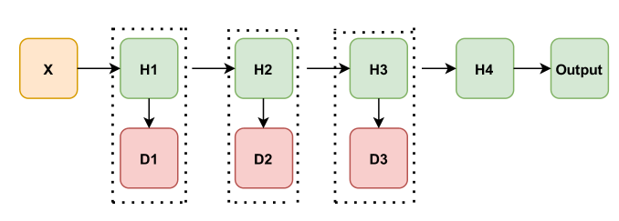
(a) MGCN(H)

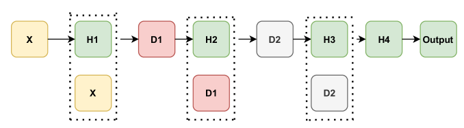
(b) MGCN(G)

Figure 1: The hierarchical GCN architecture and the global GCN architecture. $H$ represents the result of computing the graph convolutional layer, and $D$ denotes the result of the calculation of the self-attention mechanism.

   

As mentioned above, multi-scale GCN may cause over-smoothing and high computational burden. Therefore, it is necessary to aggregate multi-scale information in an effective way for better predictions. Motivated by attention mechanisms, we propose two architectures: MGCN(H) and MGCN(G) to amend the deficiency of snowball and truncated Krylov methods. These methods concatenate multi-scale feature information by self-attention mechanism, which both have the potential to be scaled to deeper architectures.

MGCN(H): In order to allow the model to use the information of different scales without increasing the computational cost, motivated by the PeleeNet (Wang et al. 2018) designed for object detection, we develop a multi-scale GCN (Fig. 2(b)), which adds an attention module in the middle of each layer. This module can expand the receptive field of the information achieved by the previous layer, concatenate the output of the previous layer and the obtained information from the attention module to the subsequent layer. Hence, this kind of approach can not only enhance the feature ability of the GCNs, but also improve the prediction accuracy, and not increase the computational burden. Let us address the detailed structure of it. The first layer is the same as conventional GCN.

$$H_{1}={\rm\sigma}(AXW_{0})$$ (4)

where $W_{0}\in\mathbb{R}^{d\times d_{0}}$ is the input-to-hidden weight matrix, $\sigma$ is the activation function (e.g. $\rm tanh$ , $\rm ReLU$ ). The attention module is computed as

$$D_{l}={\rm tanh}({\rm GNN}(H_{l},A)),l=1,2,\cdots,n-1,$$ (5)

$$C_{l}={\rm Concate}(H_{l},D_{l}),l=1,2,\cdots,n-1,$$ (6)

where $C_{l}$ are used as input to the next layer, $Concate$ stands for concatenate. Hence, $C_{\ell}$ conducts concatenation operation. Similarly, we can even perform self-attention calculations on the feature matrix $X$, and the result will be combined with itself as the input of the first layer. The computation of graph convolution for the middle layers can be casted as

$$H_{l+1}={\rm\sigma}(AC_{l}W_{l}),l=1,2,...n-1.$$ (7)

$${\rm output}={\rm softmax}(AH_{n}W_{C})$$ (8)

where $W_{l}\in\mathbb{R}^{(d_{\ell-1}+d_{\ell})\times d_{l}}$ , $W_{C}\in\mathbb{R}^{d_{n-1}\times d_{C}}$ are parameter matrices. $d_{\ell}$ is the number of output channels in the $\ell$-th layer.

MGCN(G): In Luan et al. (2019), the snowball model transfers the information of previous layer to the next layer, so that the feature information of different scales could be well used, and alleviate the vanishing gradient problem, improve prediction accuracy. However, it will cause a huge amount of calculation, and lead to the over-smoothing problem. Therefore, we propose a self-attention based multi-scale global architecture (Fig. 2(a)) that not only inherits the merits of snowball, but also overcome its shortcomings. The details are given as follows. The first layer is computed as

$$H_{1}={\rm\sigma}(AXW_{0})$$ (9)

where $W_{0}\in\mathbb{R}^{d\times d_{0}}$ are parameter matrices.

$$C_{1}={\rm Concate}(X,H_{1})$$ (10)

$$D_{1}={\rm tanh}({\rm GNN}(C_{1},A))$$ (11)

The core idea for the computation of the subsequent layers is taking a self-attention module calculation after splicing the previous results, and passing it to the next layer.

$$C_{l+1}={\rm Concate}(H_{l+1},D_{l}),l=1,2,\cdots,n-1,$$ (12)

$$D_{l+1}={\rm tanh}({\rm GNN}(C_{l+1},A)),l=1,2,\cdots,n-1,$$ (13)

$$H_{l+1}={\rm\sigma}(AD_{l}W_{l}),l=1,2,\cdots,n-1,$$ (14)

$${\rm output}={\rm softmax}(AH_{n}W_{C})$$ (15)

where $W_{l}\in\mathbb{R}^{(\sum^{\ell}_{i=0}d_{i})\times d_{l}}$ , $W_{C}\in\mathbb{R}^{d_{n-1}\times d_{C}}$ are parameter matrices. Therefore, compared to snowball and truncated Krylov methods, the difference lies in that extra attention operations, i.e., Equations (5), (10) and (12), are considered in the proposed two architectures.

Experiments

Settings

To validate the proposed global architecture and hierarchical architecture for graph representation learning, we evaluate our two multi-scale GCNs on both node classification and graph classification. All the experiments are performed under Ubuntu 16.04 in Inter CPU i6850K and 32 GB of RAM.

Datasets

We evaluate the performance of the proposed MGCN (H) and MGCN (G) on $6$ datasets with a large number of graphs ($>1k$) for the graph classification task, and $3$ commonly used citation networks for the semi-supervised node classification task. Details of the data statistics about the citation networks (graph datasets resp.) are addressed in Table 1 (Table 2 resp.)

Citation networks: The $3$ benchmark citation networks, namely, Cora, Citeseer, and Pubmed (Sen et al. 2008) contains documents as node and citation links as directed edges, which stand for the citation relationships connected to documents. The characteristics of nodes are representative words in documents, and the label rate here denotes the percentage of node tags used for training. We use undirected versions of the graphs for all the experiments although the networks are directed. In this paper, we use public splits (Yang, Cohen, and Salakhudinov 2016) approach for training.

Graph datasets: Among TU datasets (Morris et al. 2020), we select six datasets including D$\&$D, PROTEINS, MUTAGENICITY, NCI1, NCI109, and FRANKENSTEIN, where D$\&$D, PROTEINS and MUTAGENICITY contain graphs of protein structures, whilst NCI1 and NCI109 are commonly used as benchmark datasets for graph classification. FRANKENSTEIN is a set of molecular graphs with node features containing continuous values. For these $6$ datasets, we randomly select $80\%$, $10\%$, and $10\%$ of data for training, validation, and test.

Table 1: Summary of the citation networks.

Dataset	Cora	Citeseer	Pubmed
Nodes	2708	3327	19717
Edges	5429	4732	44338
Features	1433	3703	500
Classes	7	6	3
Label Rate	5.2%	3.6%	0.3%

Table 2: Summary of the datasets used for graph classification.

Dataset	D$\&$D	PROTEINS	NCI1	NCI109	FRANKENSTEIN	MUTAGENICITY
Number of Graphs	1178	1113	4110	4127	4337	4337
Avg. $\#$ of Nodes Per Graph	284.32	39.06	29.87	29.68	16.90	30.32
Avg. $\#$ of Edges Per Graph	715.66	72.82	32.30	32.13	17.88	30.77
Number of Classes	2	2	2	2	2	2

Comparison with state-of-the-art methods

We compare against $3$ classical GCNs: graph convolutional network (GCN) (Kipf and Welling 2017), graph attention network (GAT) (Veličković et al. 2018), graph sample and aggregate (GraphSAGE) (Hamilton, Ying, and Leskovec 2017). Moreover, our model are based on multi-scale tactic and self-attention mechanism. Hence, classical Chebyshev networks (Cheby) (Defferrard, Bresson, and Vandergheynst 2016), Self-Attention Graph Pooling (SAGPoolg and SAGPoolh) (Lee, Lee, and Kang 2019) and two famous multi-scale deep convolutional networks: snowball and truncated block Krylov network (Luan et al. 2019) are also considered as competitors.

Parameter settings

Node classification: For node classification task, we use RMSprop (Hinton, Srivastava, and Swersky 2012) optimizer. There are several hyperparameters, including learning rate and weight decay. The learning rate takes values from the set $\{0.01,4.7e-4,4.7e-5\}$, whilst the weight decay is chosen from the set $\{0.03,5e-3,5e-4,5e-5\}$. We choose width of hidden layers in the set $\{200,800,1600,1900,3750\}$, number of hidden layers and dropout in the set $\{1,2,...,8\}$ and $\{0,0.2\}$, respectively. To achieve good training result, we utilize adaptive number of episodes (but no more than 3000): the early stopping counter is set to be 100, the same as those described in Luan et al. (2019).

Graph classification: For graph classification task, Adam optimizer (Kingma and Ba 2015) is employed. We set learning rate $\gamma=5e-4$, pooling ratio equals to $1$, weight decay as $1e-4$, and dropout rate equals to $0.5$. The model considered in this paper has $128$ hidden units. We terminate the training if the validation loss does not improve for $50$ epochs (the maximum of epochs are set as $100K$). In addition, for the two proposed architectures, we use the MLP module in the last, and utilize the mean and the maximum readout, whilst the mean readout is employed for all the baselines.

Experimental results

As demonstrated in Fig. 1(a), the MGCN (H) and the MGCN (G) stand for hierarchical GCN architecture and the global GCN architecture, respectively. We report the accuracy, and training time. The comparison results for node classification and graph classification are summarized in Tables 3 and 4, respectively.

Table 3: Average accuracy over $10$ runs for node classification.

Method	Cora	Citeseer	Pubmed
Cheby	78.0	70.1	69.8
GCN	80.5	68.7	77.8
GAT	83.0	72.5	79.0
GraphSAGE	74.5	67.2	76.8
snowball	83.6	72.6	79.5
truncated Krylov	83.5	73.9	79.9
MGCN (H)	83.4	72.7	79.5
MGCN (G)	84.0	74.0	80.0

Table 4: Average accuracy over $10$ runs for graph classification.

Method	D$\&$D	PROTEINS	NCI1	NCI109	FRANKENSTEIN	MUTAGENICITY
GCN	73.26	75.17	76.29	75.19	62.70	79.81
GraphSAGE	75.78	74.01	74.73	74.17	63.91	78.75
GAT	77.30	74.72	74.90	75.81	59.90	78.89
SAGPool (g)	76.19	70.04	74.18	74.06	62.57	74.51
SAGPool (h)	76.45	71.86	67.45	67.86	61.73	74.71
snowball	73.95	71.43	71.53	78.02	62.30	83.68
truncated Krylov	79.54	78.85	78.16	78.16	78.16	79.54
MGCN (H)	82.53	82.07	78.10	79.31	74.48	81.15
MGCN (G)	83.91	81.84	77.24	80.23	80.00	81.15

Experimental results in Tables 3 and 4 demonstrate significant improvement of MGCN model over the baselines. Specifically, for $3$ public citation networks and $6$ graph datasets, MGCN (H) or MGCN (G) achieves impressive improvement of the accuracy on $3$ public citation datasets, and outperforms the competitors on $4$ out of $6$ datasets. Intuitively, MGCN (H) and MGCN (G) are able to enhance the performance of GCNs, and provides better qualitative results for distinct types of graph structural data.

To demonstrate the effect of the proposed two architectures related with the over-smoothing issue, we also add experiments on the over-smoothing discussion. In Fig. 2(a), Tables 5 and 6, we can observe that the proposed MGCN (H) and MGCN (G) effectively ameliorate the over-smoothing phenomenon and improve the accuracy. Even the number of layers are stacked to $30$ or $64$, the accuracy achieved is still the highest. However, the accuracy results of snowball and truncated Krylov methods drop rapidly when the depth of the network is increased.

Table 7 displays the comparison of training time between MGCN (H), MGCN (G) and two recently proposed multi-scale deep convolutional networks, namely, snowball and truncated Krylov. We can see that MGCN (G) runs faster on Cora and Citeseer datasets. We think the reason is that the self-attention mechanism allow the model to focus on using multi-scale information, instead of accumulating the information from the previous layer to the next layer mechanically, which can achieve much less computational cost.

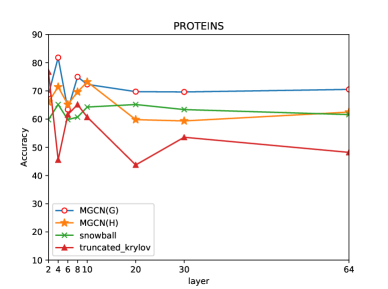
(a) Accuracy on PROTEINS dataset with different layers

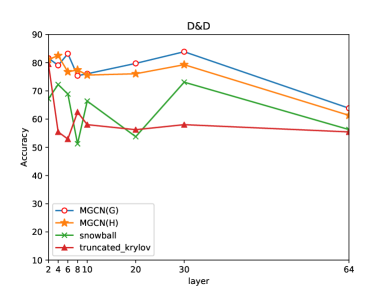
(b) Accuracy on D$\&$D dataset with different layers

Figure 2: The accuracy on D$\&$D (a) and PROTEINS (b) datasets with different layers.

   

Table 5: Accuracy on PROTEINS dataset using distinct number of layers.

Method	2-layer	4-layer	6-layer	8-layer	10-layer	20-layer	30-layer	64-layer
snowball	59.82	65.18	59.82	60.71	64.29	65.18	63.39	61.61
truncated Krylov	76.78	45.54	61.61	65.18	60.71	43.75	53.57	48.21
MGCN(H)	66.07	71.43	65.18	69.64	73.21	59.82	59.36	62.50
MGCN(G)	68.75	81.84	63.39	75.00	72.32	69.75	69.64	70.54

Table 6: Accuracy on D$\&$D dataset using distinct number of layers.

Method	2-layer	4-layer	6-layer	8-layer	10-layer	20-layer	30-layer	64-layer
snowball	67.23	72.27	68.91	51.26	66.39	53.78	73.11	56.30
truncated Krylov	79.54	55.46	52.94	62.50	58.04	56.25	58.04	55.46
MGCN(H)	81.15	82.53	76.78	77.47	75.63	76.09	79.31	61.34
MGCN(G)	81.61	79.08	83.22	75.40	76.09	79.77	83.91	63.87

Table 7: Average training time (s) comparison with snowball and truncated Krylov methods on $3$ citation networks.

Method	Cora	Citeseer	Pubmed
snowball	484.10	1228.57	265.41
truncated Krylov	213.81	1194.94	254.85
MGCN (H)	158.88	304.53	219.92
MGCN (G)	184.90	269.74	184.60

Conclusion and future work

In this paper, we propose two novel multi-scale graph convolutional networks based on self-attention. Our methods can not only utilize multi-scale information to improve the expressive power of GCNs, but also alleviate the problems of large scale calculation, and over-smoothing of the previous multi-scale graph convolution model. We validate the performance of the proposed frameworks on both node classification and graph classification tasks. Our framework is universal, and one can replace the self-attention module via other graph pooling methods, for instance, gPool (Gao and Ji 2019), SortPool (Zhang et al. 2018), DiffPool (Ying et al. 2018), Set2Set (Vinyals, Bengio, and Kudlur 2016) etc.

References

- Bianchi et al. (2021) Bianchi, F. M.; Grattarola, D.; Livi, L.; and Alippi, C. 2021. Graph neural networks with convolutional arma filters. IEEE Transactions on Pattern Analysis and Machine Intelligence.
- Bruna et al. (2014) Bruna, J.; Zaremba, W.; Szlam, A.; and Lecun, Y. 2014. Spectral Networks and Locally Connected Networks on Graphs. In ICLR.
- Casas et al. (2020) Casas, S.; Gulino, C.; Liao, R.; and Urtasun, R. 2020. SpAGNN: Spatially-Aware Graph Neural Networks for Relational Behavior Forecasting from Sensor Data. 2020 IEEE International Conference on Robotics and Automation (ICRA), 9491–9497.
- Defferrard, Bresson, and Vandergheynst (2016) Defferrard, M.; Bresson, X.; and Vandergheynst, P. 2016. Convolutional neural networks on graphs with fast localized spectral filtering. NeurIPS, 29: 3844–3852.
- Gao and Ji (2019) Gao, H.; and Ji, S. 2019. Graph u-nets. In ICML, 2083–2092.
- Hamilton, Ying, and Leskovec (2017) Hamilton, W. L.; Ying, R.; and Leskovec, J. 2017. Inductive representation learning on large graphs. In NeurIPS, 1025–1035.
- He et al. (2021) He, M.; Wei, Z.; Huang, Z.; and Xu, H. 2021. BernNet: Learning Arbitrary Graph Spectral Filters via Bernstein Approximation. arXiv preprint arXiv:2106.10994.
- Hinton, Srivastava, and Swersky (2012) Hinton, G.; Srivastava, N.; and Swersky, K. 2012. Neural networks for machine learning lecture 6a overview of mini-batch gradient descent. Cited on, 14(8): 2.
- Kingma and Ba (2015) Kingma, D.; and Ba, J. 2015. Adam: A Method for Stochastic Optimization. In ICLR.
- Kipf and Welling (2017) Kipf, T.; and Welling, M. 2017. Semi-Supervised Classification with Graph Convolutional Networks. In ICLR.
- Lee, Lee, and Kang (2019) Lee, J.; Lee, I.; and Kang, J. 2019. Self-attention graph pooling. In ICML, 3734–3743.
- Liao et al. (2019) Liao, R.; Zhao, Z.; Urtasun, R.; and Zemel, R. 2019. LanczosNet: Multi-Scale Deep Graph Convolutional Networks. In ICLR.
- Luan et al. (2019) Luan, S.; Zhao, M.; Chang, X.-W.; and Precup, D. 2019. Break the Ceiling: Stronger Multi-scale Deep Graph Convolutional Networks. In NeurIPS, volume 32.
- Morris et al. (2020) Morris, C.; Kriege, N. M.; Bause, F.; Kersting, K.; and Neumann, M. 2020. TUDataset: A collection of benchmark datasets for learning with graphs.
- Rong et al. (2020) Rong, Y.; Huang, W.; Xu, T.; and Huang, J. 2020. DropEdge: Towards Deep Graph Convolutional Networks on Node Classification. In ICLR.
- Sen et al. (2008) Sen, P.; Namata, G.; Bilgic, M.; Getoor, L.; Gallagher, B.; and Eliassi-Rad, T. 2008. Collective Classification in Network Data. AI Mag., 29: 93–106.
- Stokes et al. (2020) Stokes, J. M.; Yang, K.; Swanson, K.; Jin, W.; and Collins, J. J. 2020. A Deep Learning Approach to Antibiotic Discovery. Cell, 180(4): 688–702.e13.
- Sun et al. (2020) Sun, J.; Guo, W.; Zhang, D.; Zhang, Y.; Regol, F.; Hu, Y.; Guo, H.; Tang, R.; Yuan, H.; He, X.; and Coates, M. 2020. A Framework for Recommending Accurate and Diverse Items Using Bayesian Graph Convolutional Neural Networks. Proceedings of the 26th ACM SIGKDD International Conference on Knowledge Discovery & Data Mining.
- Sun, Lin, and Zhu (2021) Sun, K.; Lin, Z.; and Zhu, Z. 2021. AdaGCN: Adaboosting Graph Convolutional Networks into Deep Models. In ICLR.
- Vaswani et al. (2017) Vaswani, A.; Shazeer, N.; Parmar, N.; Uszkoreit, J.; Jones, L.; Gomez, A. N.; Kaiser, Ł.; and Polosukhin, I. 2017. Attention is all you need. In NeurIPS, 5998–6008.
- Veličković et al. (2018) Veličković, P.; Cucurull, G.; Casanova, A.; Romero, A.; Li, P.; and Bengio, Y. 2018. Graph Attention Networks. In ICLR.
- Vinyals, Bengio, and Kudlur (2016) Vinyals, O.; Bengio, S.; and Kudlur, M. 2016. Order Matters: Sequence to sequence for sets. In ICLR.
- Wang et al. (2018) Wang, R.; Li, X.; Ao, S.; and Ling, C. 2018. Pelee: A Real-Time Object Detection System on Mobile Devices. In NeurIPS.
- Xu et al. (2019a) Xu, B.; Shen, H.; Cao, Q.; Qiu, Y.; and Cheng, X. 2019a. Graph Wavelet Neural Network. In ICLR.
- Xu et al. (2019b) Xu, K.; Hu, W.; Leskovec, J.; and Jegelka, S. 2019b. How Powerful are Graph Neural Networks? In ICLR.
- Xu et al. (2018) Xu, K.; Li, C.; Tian, Y.; Sonobe, T.; Kawarabayashi, K.-i.; and Jegelka, S. 2018. Representation learning on graphs with jumping knowledge networks. In ICML, 5453–5462.
- Yang, Cohen, and Salakhudinov (2016) Yang, Z.; Cohen, W.; and Salakhudinov, R. 2016. Revisiting semi-supervised learning with graph embeddings. In ICML, 40–48.
- Yao, Mao, and Luo (2019) Yao, L.; Mao, C.; and Luo, Y. 2019. Graph Convolutional Networks for Text Classification. In AAAI.
- Ying et al. (2018) Ying, R.; You, J.; Morris, C.; Ren, X.; Hamilton, W. L.; and Leskovec, J. 2018. Hierarchical Graph Representation Learning with Differentiable Pooling.
- Zhang et al. (2018) Zhang, M.; Cui, Z.; Neumann, M.; and Chen, Y. 2018. An end-to-end deep learning architecture for graph classification. In AAAI.
- Zhu (2012) Zhu, J. 2012. Max-Margin Nonparametric Latent Feature Models for Link Prediction. In ICML.